Slide 1 Searching: Deterministic single-agent Andrew W. Moore Professor School of Computer Science...
89
Slide 1 Searching: Deterministic single-agent Andrew W. Moore Professor School of Computer Science Carnegie Mellon University www.cs.cmu.edu/~awm [email protected] 412-268-7599 Note to other teachers and users of these slides. Andrew would be delighted if you found this source material useful in giving your own lectures. Feel free to use these slides verbatim, or to modify them to fit your own needs. PowerPoint originals are available. If you make use of a significant portion of these slides in your own lecture, please include this message, or the following link to the source repository of Andrew’s tutorials: http://www.cs.cmu.edu/~awm/tutorials . Comments and corrections gratefully
-
Upload
lindsey-jones -
Category
Documents
-
view
214 -
download
0
Transcript of Slide 1 Searching: Deterministic single-agent Andrew W. Moore Professor School of Computer Science...

Slide 1
Searching: Deterministic single-agent
Andrew W. MooreProfessor
School of Computer ScienceCarnegie Mellon University
www.cs.cmu.edu/[email protected]
412-268-7599
Note to other teachers and users of these slides. Andrew would be delighted if you found this source material useful in giving your own lectures. Feel free to use these slides verbatim, or to modify them to fit your own needs. PowerPoint originals are available. If you make use of a significant portion of these slides in your own lecture, please include this message, or the following link to the source repository of Andrew’s tutorials: http://www.cs.cmu.edu/~awm/tutorials . Comments and corrections gratefully received.

Slide 2
Overview
• Deterministic, single-agent, search problems• Breadth First Search• Optimality, Completeness, Time and Space
complexity• Search Trees• Depth First Search• Iterative Deepening• Best First “Greedy” Search

Slide 3
A search problem
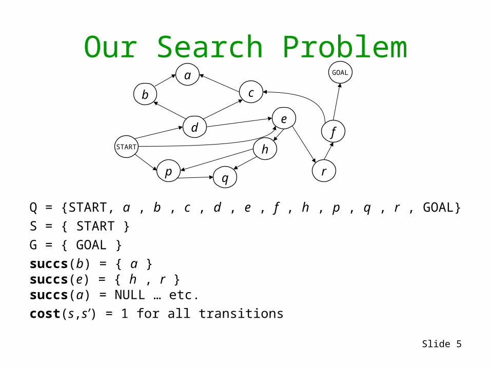
How do we get from S to G? And what’s the smallest possible number of transitions?
START
GOAL
d
b
pq
c
e
h
a
f
r

Slide 4
Formalizing a search problemA search problem has five components:Q , S , G , succs , cost• Q is a finite set of states.• S Q is a non-empty set of start states.• G Q is a non-empty set of goal states.• succs : Q P(Q) is a function which takes a state as
input and returns a set of states as output. succs(s) means “the set of states you can reach from s in one step”.
• cost : Q , Q Positive Number is a function which takes two states, s and s’, as input. It returns the one-step cost of traveling from s to s’. The cost function is only defined when s’ is a successor state of s.
Slide 5
Our Search Problem
Q = {START, a , b , c , d , e , f , h , p , q , r , GOAL}
S = { START }
G = { GOAL }
succs(b) = { a }succs(e) = { h , r }succs(a) = NULL … etc.
cost(s,s’) = 1 for all transitions
START
GOAL
d
b
p q
c
e
h
a
f
r

Slide 6
Our Search Problem
Q = {START, a , b , c , d , e , f , h , p , q , r , GOAL}
S = { START }
G = { GOAL }
succs(b) = { a }succs(e) = { h , r }succs(a) = NULL … etc.
cost(s,s’) = 1 for all transitions
START
GOAL
d
b
p q
c
e
h
a
f
r
Why do we care? What
problems are like this?

Slide 7
Search Problems

Slide 8
More Search ProblemsScheduling
8-Queens
What next?
Slide 9
More Search ProblemsScheduling
8-Queens
What next?
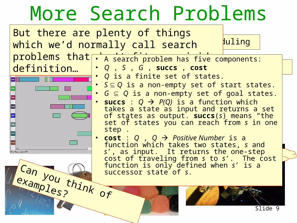
But there are plenty of things which we’d normally call search problems that don’t fit our rigid definition… • A search problem has five components:
• Q , S , G , succs , cost• Q is a finite set of states.• S Q is a non-empty set of start states.• G Q is a non-empty set of goal states.• succs : Q P(Q) is a function which takes a
state as input and returns a set of states as output. succs(s) means “the set of states you can reach from s in one step”.
• cost : Q , Q Positive Number is a function which takes two states, s and s’, as input. It returns the one-step cost of traveling from s to s’. The cost function is only defined when s’ is a successor state of s.
Can you think of examples?

Slide 10
Our definition excludes…

Slide 11
Our definition excludes…Game against
adversary
ChanceHidden State
Continuum (infinite number) of states
All of the above, plus distributed team control

Slide 12
Breadth First Search
Label all states that are reachable from S in 1 step but aren’t reachable in less than 1 step.
Then label all states that are reachable from S in 2 steps but aren’t reachable in less than 2 steps.
Then label all states that are reachable from S in 3 steps but aren’t reachable in less than 3 steps.
Etc… until Goal state reached.
START
GOAL
d
b
p q
c
e
h
a
f
r

Slide 13
START
GOAL
d
b
pq
c
e
h
a
f
r
Breadth-first Search
0 steps from start

Slide 14
START
GOAL
d
b
pq
c
e
h
a
f
r
Breadth-first Search
0 steps from start
1 step from start

Slide 15
START
GOAL
d
b
pq
c
e
h
a
f
r
Breadth-first Search
0 steps from start
1 step from start
2 steps from start

Slide 16
START
GOAL
d
b
pq
c
e
h
a
f
r
Breadth-first Search
0 steps from start
1 step from start
2 steps from start
3 steps from start

Slide 17
START
GOAL
d
b
pq
c
e
h
a
f
r
Breadth-first Search
0 steps from start
1 step from start
2 steps from start
3 steps from start
4 steps from start
Slide 18
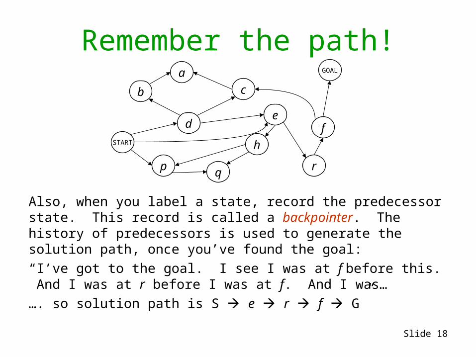
Remember the path!
Also, when you label a state, record the predecessor state. This record is called a backpointer. The history of predecessors is used to generate the solution path, once you’ve found the goal:
“I’ve got to the goal. I see I was at f before this. And I was at r before I was at f. And I was…
…. so solution path is S e r f G”
START
GOAL
d
b
p q
c
e
h
a
f
r
Slide 19
START
GOAL
d
b
pq
c
e
h
a
f
r
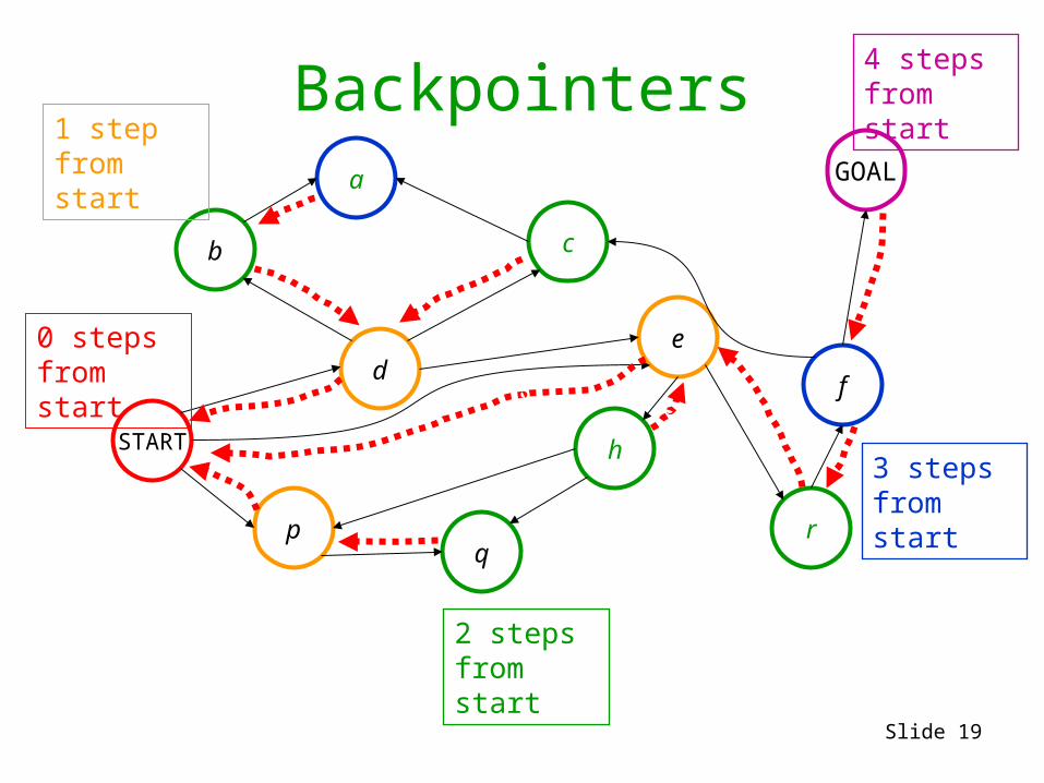
Backpointers
0 steps from start
1 step from start
2 steps from start
3 steps from start
4 steps from start
Slide 20
START
GOAL
d
b
pq
c
e
h
a
f
r
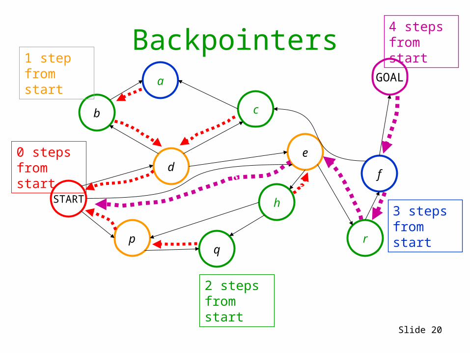
Backpointers
0 steps from start
1 step from start
2 steps from start
3 steps from start
4 steps from start

Slide 21
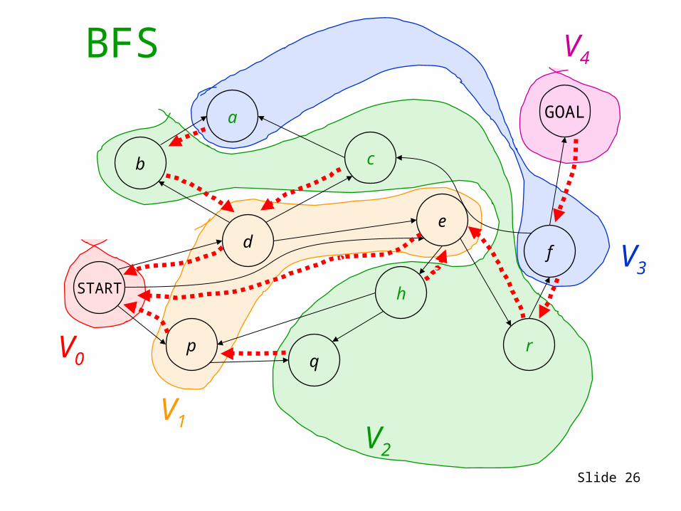
Starting Breadth First SearchFor any state s that we’ve labeled, we’ll remember:
•previous(s) as the previous state on a shortest path from START state to s.
On the kth iteration of the algorithm we’ll begin with Vk defined as the set of those states for which the shortest path from the start costs exactly k steps
Then, during that iteration, we’ll compute Vk+1, defined as the set of those states for which the shortest path from the start costs exactly k+1 steps
We begin with k = 0, V0 = {START} and we’ll define, previous(START) = NULL
Then we’ll add in things one step from the START into V1. And we’ll keep going.

Slide 22
START
GOAL
d
b
pq
c
e
h
a
f
r
BFS
V0

Slide 23
START
GOAL
d
b
pq
c
e
h
a
f
r
BFS
V0
V1

Slide 24
START
GOAL
d
b
pq
c
e
h
a
f
r
BFS
V0
V1V2

Slide 25
START
GOAL
d
b
pq
c
e
h
a
f
r
BFS
V0
V1V2
V3
Slide 26
START
GOAL
d
b
pq
c
e
h
a
f
r
BFS V4
V0
V1V2
V3

Slide 27
Breadth First SearchV0 := S (the set of start states)
previous(START) := NIL
k := 0
while (no goal state is in Vk and Vk is not empty) do
Vk+1 := empty set
For each state s in Vk
For each state s’ in succs(s)
If s’ has not already been labeled
Set previous(s’) := s
Add s’ into Vk+1
k := k+1
If Vk is empty signal FAILURE
Else build the solution path thus: Let Si be the ith state in the shortest path. Define Sk = GOAL, and forall i <= k, define Si-1 = previous(Si).

Slide 28
START
GOAL
d
b
pq
c
e
h
a
f
r
BFS V4
V0
V1V2
V3Suppose your search space conveniently
allowed you to obtain predecessors(state).
• Can you think of a different way to do BFS?
• And would you be able to avoid storing
something that we’d previously had to
store?

Slide 29
Another way: Work back
Label all states that can reach G in 1 step but can’t reach it in less than 1 step.
Label all states that can reach G in 2 steps but can’t reach it in less than 2 steps.
Etc. … until start is reached.
“number of steps to goal” labels determine the shortest path. Don’t need extra bookkeeping info.
START
GOAL
d
b
p q
c
e
h
a
f
r

Slide 30
Breadth First Details• It is fine for there to be more than one goal state.• It is fine for there to be more than one start state.• This algorithm works forwards from the start. Any
algorithm which works forwards from the start is said to be forward chaining.
• You can also work backwards from the goal. This algorithm is very similar to Dijkstra’s algorithm.
• Any algorithm which works backwards from the goal is said to be backward chaining.
• Backward versus forward. Which is better?

Slide 31
Costs on transitions
Notice that BFS finds the shortest path in terms of number of transitions. It does not find the least-cost path.
We will quickly review an algorithm which does find the least-cost path. On the kth iteration, for any state S, write g(s) as the least-cost path to S in k or fewer steps.
START
GOAL
d
b
pq
c
e
h
a
f
r
2
9 9
81
1
2
3
534
4
15
1
5 5
2

Slide 32
Least Cost Breadth FirstVk = the set of states which can be reached in exactly k steps, and for which the least-cost k-step path is less cost than any path of length less than k. In other words, Vk = the set of states whose values changed on the previous iteration.
V0 := S (the set of start states)previous(START) := NILg(START) = 0k := 0while (Vk is not empty) do
Vk+1 := empty setFor each state s in Vk
For each state s’ in succs(s)If s’ has not already been labeledOR if g(s) + Cost(s,s’) < g(s’)
Set previous(s’) := sSet g(s’) := g(s) + Cost(s,s’)Add s’ into Vk+1
k := k+1If GOAL not labeled, exit signaling FAILUREElse build the solution path thus: Let Sk be the kth state in the shortest path. Define Sk = GOAL, and forall i <= k, define Si-1 = previous(Si).

Slide 33
Uniform-Cost Search
• A conceptually simple BFS approach when there are costs on transitions
• It uses priority queues

Slide 34
Priority Queue RefresherA priority queue is a data structure in which you can insert and retrieve (thing, value) pairs with the following operations:
Init-PriQueue(PQ) initializes the PQ to be empty.
Insert-PriQueue(PQ, thing, value) inserts (thing, value) into the queue.
Pop-least(PQ) returns the (thing, value) pair with the lowest value, and removes it from the queue.

Slide 35
Priority Queue RefresherA priority queue is a data structure in which you can insert and retrieve (thing, value) pairs with the following operations:
Priority Queues can be implemented in such a way that the cost of the insert and pop operations are
For more details, see Knuth or Sedgwick or basically any book with the word “algorithms” prominently appearing in the title.
Init-PriQueue(PQ) initializes the PQ to be empty.
Insert-PriQueue(PQ, thing, value) inserts (thing, value) into the queue.
Pop-least(PQ) returns the (thing, value) pair with the lowest value, and removes it from the queue.
Very cheap (though not absolutely, incredibly cheap!)
O(log(number of things in priority queue))

Slide 36
Uniform-Cost Search• A conceptually simple BFS approach when
there are costs on transitions• It uses a priority queue
PQ = Set of states that have been expanded or are awaiting expansion
Priority of state s = g(s) = cost of getting to s using path implied by backpointers.

Slide 37
Starting UCS
PQ = { (S,0) }
START
GOAL
d
b
pq
c
e
h
a
f
r
2
9 9
81
1
2
3
5
34
4
15
1
25
2

Slide 38
PQ = { (S,0) }
START
GOAL
d
b
pq
c
e
h
a
f
r
2
9 9
81
1
2
3
5
34
4
15
1
25
2
Iteration:1. Pop least-cost state from PQ2. Add successors
UCS Iterations

Slide 39
PQ = { (p,1), (d,3) , (e,9) }
START
GOAL
d
b
pq
c
e
h
a
f
r
2
9 9
81
1
2
3
5
34
4
15
1
25
2
Iteration:1. Pop least-cost state from PQ2. Add successors
UCS Iterations
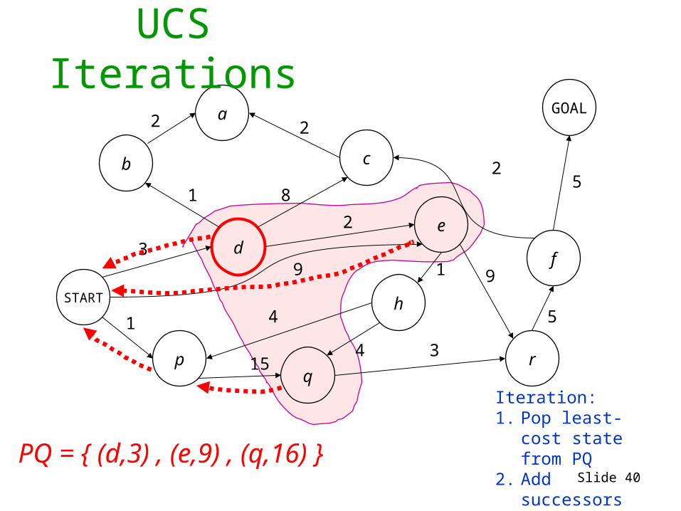
Slide 40
PQ = { (d,3) , (e,9) , (q,16) }
START
GOAL
d
b
pq
c
e
h
a
f
r
2
9 9
81
1
2
3
5
34
4
15
1
25
2
Iteration:1. Pop least-cost
state from PQ2. Add successors
UCS Iterations
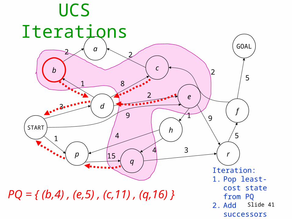
Slide 41
PQ = { (b,4) , (e,5) , (c,11) , (q,16) }
START
GOAL
d
b
pq
c
e
h
a
f
r
2
9 9
81
1
2
3
5
34
4
15
1
25
2
Iteration:1. Pop least-cost
state from PQ2. Add successors
UCS Iterations
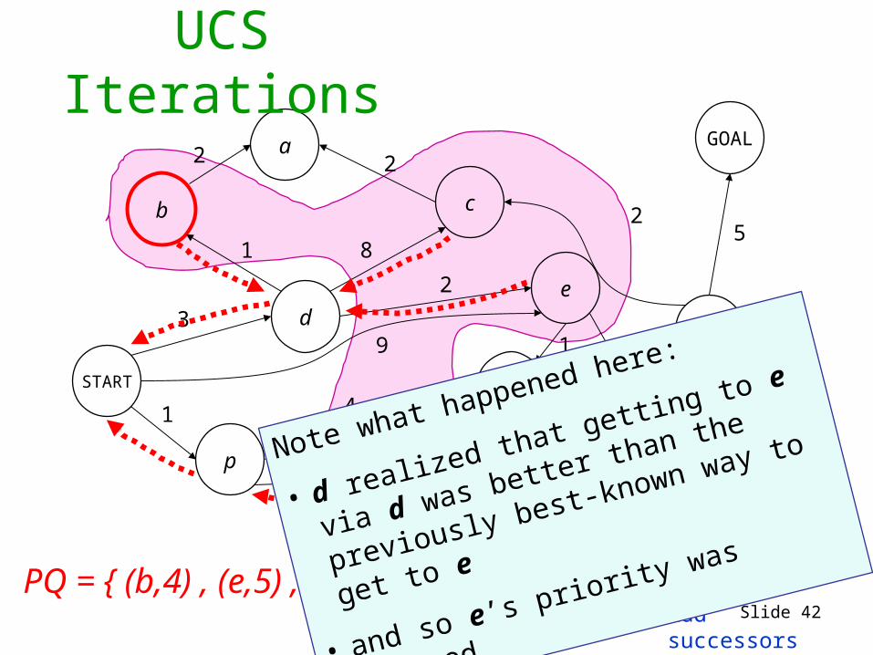
Slide 42
PQ = { (b,4) , (e,5) , (c,11) , (q,16) }
START
GOAL
d
b
pq
c
e
h
a
f
r
2
9 9
81
1
2
3
5
34
4
15
1
25
2
Iteration:1. Pop least-cost
state from PQ2. Add successors
UCS Iterations
Note what happened here:
• d realized that getting to e via d was
better than the previously best-known
way to get to e
• and so e’s priority was changed

Slide 43
PQ = { (e,5) , (a,6) , (c,11) , (q,16) }
START
GOAL
d
b
pq
c
e
h
a
f
r
2
9 9
81
1
2
3
5
34
4
15
1
25
2
Iteration:1. Pop least-cost
state from PQ2. Add successors
UCS Iterations
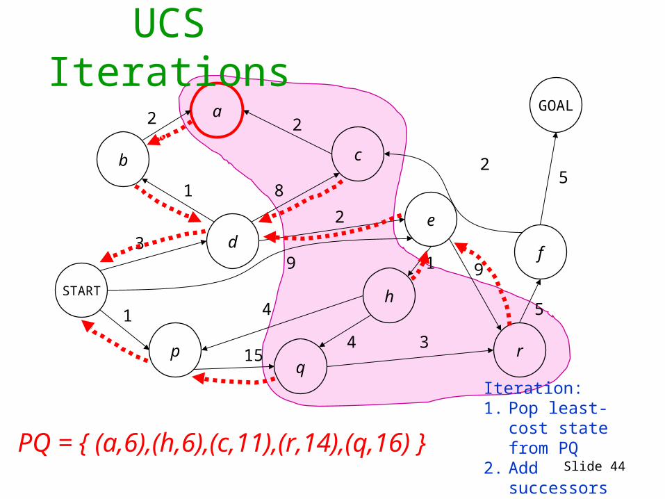
Slide 44
PQ = { (a,6),(h,6),(c,11),(r,14),(q,16) }
START
GOAL
d
b
pq
c
e
h
a
f
r
2
9 9
81
1
2
3
5
34
4
15
1
25
2
Iteration:1. Pop least-cost
state from PQ2. Add successors
UCS Iterations
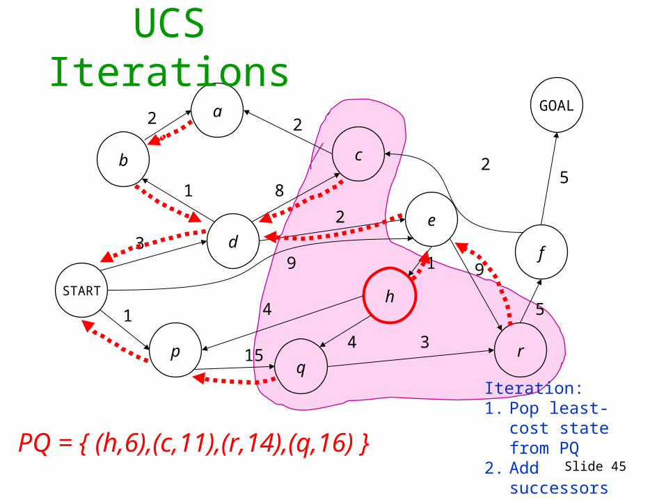
Slide 45
PQ = { (h,6),(c,11),(r,14),(q,16) }
START
GOAL
d
b
pq
c
e
h
a
f
r
2
9 9
81
1
2
3
5
34
4
15
1
25
2
Iteration:1. Pop least-cost
state from PQ2. Add successors
UCS Iterations

Slide 46
PQ = { (q,10), (c,11),(r,14) }
START
GOAL
d
b
pq
c
e
h
a
f
r
2
9 9
81
1
2
3
5
34
4
15
1
25
2
Iteration:1. Pop least-cost
state from PQ2. Add successors
UCS Iterations
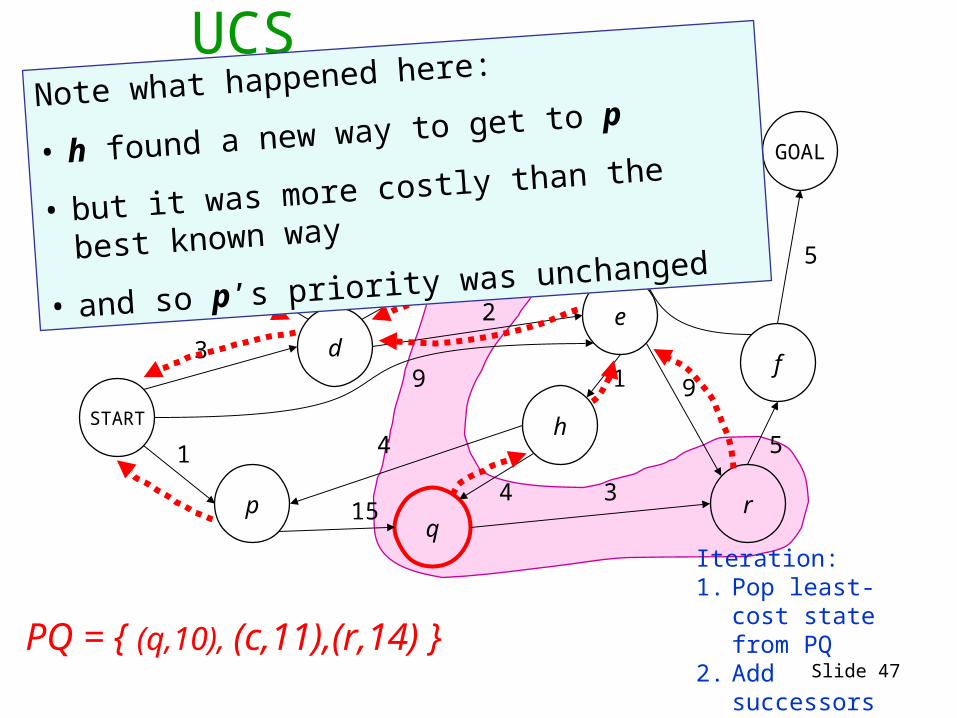
Slide 47
PQ = { (q,10), (c,11),(r,14) }
START
GOAL
d
b
pq
c
e
h
a
f
r
2
9 9
81
1
2
3
5
34
4
15
1
25
2
Iteration:1. Pop least-cost
state from PQ2. Add successors
UCS IterationsNote what happened here:
• h found a new way to get to p
• but it was more costly than the best known way
• and so p’s priority was unchanged
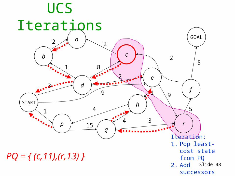
Slide 48
PQ = { (c,11),(r,13) }
START
GOAL
d
b
pq
c
e
h
a
f
r
2
9 9
81
1
2
3
5
34
4
15
1
25
2
Iteration:1. Pop least-cost
state from PQ2. Add successors
UCS Iterations

Slide 49
PQ = { (r,13) }
START
GOAL
d
b
pq
c
e
h
a
f
r
2
9 9
81
1
2
3
5
34
4
15
1
25
2
Iteration:1. Pop least-cost
state from PQ2. Add successors
UCS Iterations
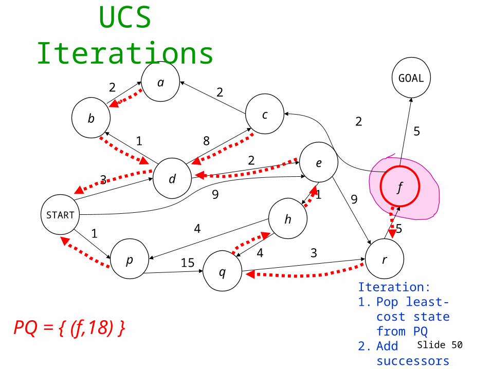
Slide 50
PQ = { (f,18) }
START
GOAL
d
b
pq
c
e
h
a
f
r
2
9 9
81
1
2
3
5
34
4
15
1
25
2
Iteration:1. Pop least-cost
state from PQ2. Add successors
UCS Iterations

Slide 51
PQ = { (G,23) }
START
GOAL
d
b
pq
c
e
h
a
f
r
2
9 9
81
1
2
3
5
34
4
15
1
25
2
Iteration:1. Pop least-cost
state from PQ2. Add successors
UCS Iterations

Slide 52
PQ = { (G,23) }
START
GOAL
d
b
pq
c
e
h
a
f
r
2
9 9
81
1
2
3
5
34
4
15
1
25
2
Iteration:1. Pop least-cost
state from PQ2. Add successors
UCS IterationsQuestion: Is “terminate as soon as you discover
the goal” the right stopping criterion?

Slide 53
PQ = { }
START
GOAL
d
b
pq
c
e
h
a
f
r
2
9 9
81
1
2
3
5
34
4
15
1
25
2
Iteration:1. Pop least-cost
state from PQ2. Add successors
UCS terminates
Terminate only once the goal is popped from the
priority queue. Else we may miss a shorter path.

Slide 54
Judging a search algorithm• Completeness: is the algorithm guaranteed to find a solution
if a solution exists?• Guaranteed to find optimal? (will it find the least cost path?)• Algorithmic time complexity• Space complexity (memory use)
Variables:
N number of states in the problem
B the average branching factor (the average number of successors) (B>1)
L the length of the path from start to goal with the shortest number of steps
How would we judge our algorithms?

Slide 55
Judging a search algorithmN number of states in the problem
B the average branching factor (the average number of successors) (B>1)
L the length of the path from start to goal with the shortest number of steps
Q the average size of the priority queue
Algorithm Complete
Optimal Time Space
BFS Breadth First Search
Y if all transitions same cost
O(min(N,BL)) O(min(N,BL))
LCBFS Least Cost BFS
Y Y O(min(N,BL)) O(min(N,BL))
UCS Uniform Cost Search
Y Y O(log(Q) * min(N,BL)) O(min(N,BL))

Slide 56
Judging a search algorithmN number of states in the problem
B the average branching factor (the average number of successors) (B>1)
L the length of the path from start to goal with the shortest number of steps
Q the average size of the priority queue
Algorithm Complete
Optimal Time Space
BFS Breadth First Search
Y if all transitions same cost
O(min(N,BL)) O(min(N,BL))
LCBFS Least Cost BFS
Y Y O(min(N,BL)) O(min(N,BL))
UCS Uniform Cost Search
Y Y O(log(Q) * min(N,BL)) O(min(N,BL))

Slide 57
Search Tree Representation
START
GOAL
d
b
p q
c
e
h
a
f
r
What order do we go through
the search tree with BFS?
Slide 58
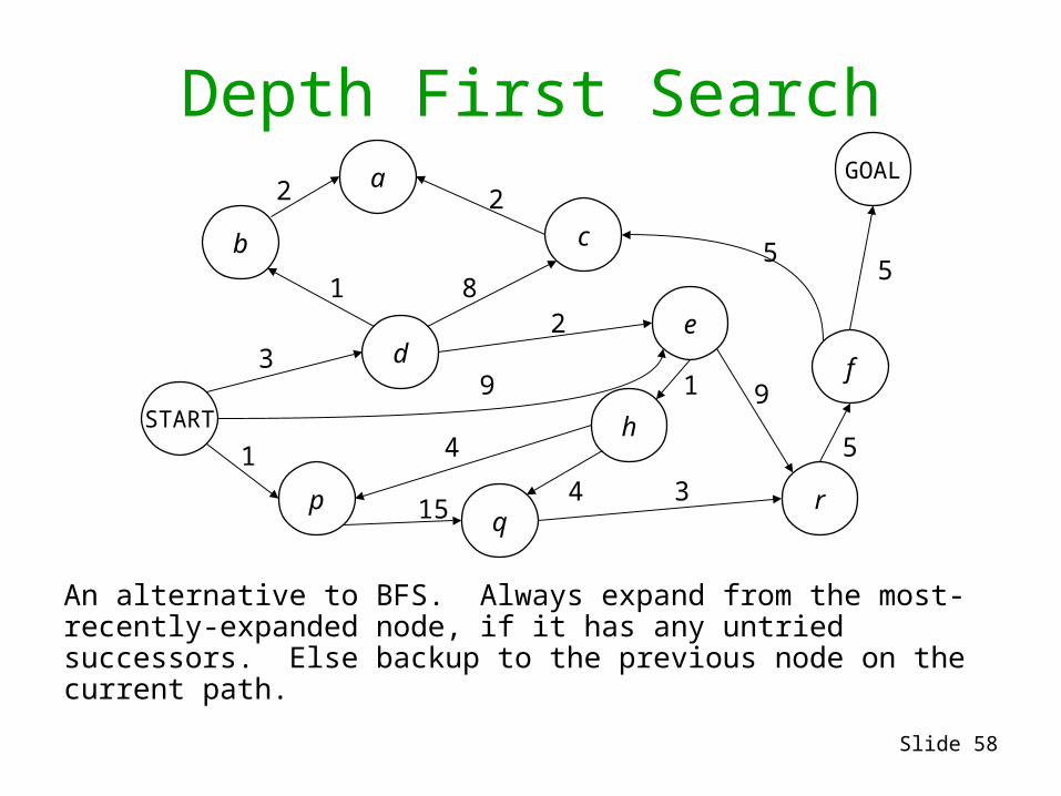
Depth First Search
An alternative to BFS. Always expand from the most-recently-expanded node, if it has any untried successors. Else backup to the previous node on the current path.
START
GOAL
d
b
pq
c
e
h
a
f
r
2
9 9
81
1
2
3
5
34
4
15
1
55
2

Slide 59
DFS in action
STARTSTART dSTART d bSTART d b aSTART d cSTART d c aSTART d eSTART d e rSTART d e r fSTART d e r f cSTART d e r f c aSTART d e r f GOAL
START
GOAL
d
b
p q
c
e
h
a
f
r

Slide 60
DFS Search tree traversal
START
GOAL
d
b
p q
c
e
h
a
f
rCan you draw in the order in which the search-tree nodes are visited?
Slide 61
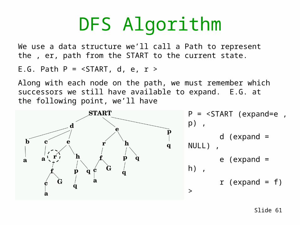
DFS AlgorithmWe use a data structure we’ll call a Path to represent the , er, path from the START to the current state.
E.G. Path P = <START, d, e, r >
Along with each node on the path, we must remember which successors we still have available to expand. E.G. at the following point, we’ll have
P = <START (expand=e , p) ,
d (expand = NULL) ,
e (expand = h) ,
r (expand = f) >

Slide 62
DFS AlgorithmLet P = <START (expand = succs(START))>While (P not empty and top(P) not a goal)
if expand of top(P) is emptythen
remove top(P) (“pop the stack”)else
let s be a member of expand of top(P)remove s from expand of top(P)make a new item on the top of path P:
s (expand = succs(s))If P is empty
return FAILUREElse
return the path consisting of states in P
This algorithm can be written neatly with recursion, i.e. using the program stack to implement P.

Slide 63
Judging a search algorithmN number of states in the problem
B the average branching factor (the average number of successors) (B>1)
L the length of the path from start to goal with the shortest number of steps
Q the average size of the priority queue
Algorithm Complete
Optimal Time Space
BFS Breadth First Search
Y if all transitions same cost
O(min(N,BL)) O(min(N,BL))
LCBFS Least Cost BFS
Y Y O(min(N,BL)) O(min(N,BL))
UCS Uniform Cost Search
Y Y O(log(Q) * min(N,BL)) O(min(N,BL))
DFS Depth First Search
N N N/A N/A
Slide 64
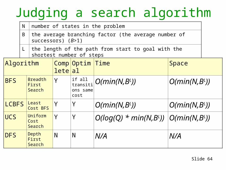
Judging a search algorithmN number of states in the problem
B the average branching factor (the average number of successors) (B>1)
L the length of the path from start to goal with the shortest number of steps
Q the average size of the priority queue
Algorithm Complete
Optimal Time Space
BFS Breadth First Search
Y if all transitions same cost
O(min(N,BL)) O(min(N,BL))
LCBFS Least Cost BFS
Y Y O(min(N,BL)) O(min(N,BL))
UCS Uniform Cost Search
Y Y O(log(Q) * min(N,BL)) O(min(N,BL))
DFS Depth First Search
N N N/A N/A

Slide 65
Judging a search algorithmN number of states in the problem
B the average branching factor (the average number of successors) (B>1)
L the length of the path from start to goal with the shortest number of steps
LMAX Length of longest path from start to anywhere
Q the average size of the priority queue
Algorithm Complete
Optimal Time Space
BFS Breadth First Search
Y if all transitions same cost
O(min(N,BL)) O(min(N,BL))
LCBFS Least Cost BFS
Y Y O(min(N,BL)) O(min(N,BL))
UCS Uniform Cost Search
Y Y O(log(Q) * min(N,BL)) O(min(N,BL))
DFS** Depth First Search
Y N O(BLMAX) O(LMAX)
Assuming Acyclic Search Space

Slide 66
Judging a search algorithmN number of states in the problem
B the average branching factor (the average number of successors) (B>1)
L the length of the path from start to goal with the shortest number of steps
LMAX Length of longest path from start to anywhere
Q the average size of the priority queue
Algorithm Complete
Optimal Time Space
BFS Breadth First Search
Y if all transitions same cost
O(min(N,BL)) O(min(N,BL))
LCBFS Least Cost BFS
Y Y O(min(N,BL)) O(min(N,BL))
UCS Uniform Cost Search
Y Y O(log(Q) * min(N,BL)) O(min(N,BL))
DFS** Depth First Search
Y N O(BLMAX) O(LMAX)
Assuming Acyclic Search Space

Slide 67
Questions to ponder
• How would you prevent DFS from looping?
• How could you force it to give an optimal solution?

Slide 68
Questions to ponder
• How would you prevent DFS from looping?
• How could you force it to give an optimal solution?
Answer 1:
PC-DFS (Path Checking DFS):
Don’t recurse on a state if that state is already in the current path
Answer 2:
MEMDFS (Memoizing DFS):
Remember all states expanded so far. Never expand anything twice.

Slide 69
Questions to ponder
• How would you prevent DFS from looping?
• How could you force it to give an optimal solution?
Answer 1:
PC-DFS (Path Checking DFS):
Don’t recurse on a state if that state is already in the current path
Answer 2:
MEMDFS (Memoizing DFS):
Remember all states expanded so far. Never expand anything twice.

Slide 70
Questions to ponder
• How would you prevent DFS from looping?
• How could you force it to give an optimal solution?
Answer 1:
PC-DFS (Path Checking DFS):
Don’t recurse on a state if that state is already in the current path
Answer 2:
MEMDFS (Memoizing DFS):
Remember all states expanded so far. Never expand anything twice.
Are there occasions when PCDFS is
better than MEMDFS?
Are there occasions when MEMDFS
is better than PCDFS?
Slide 71
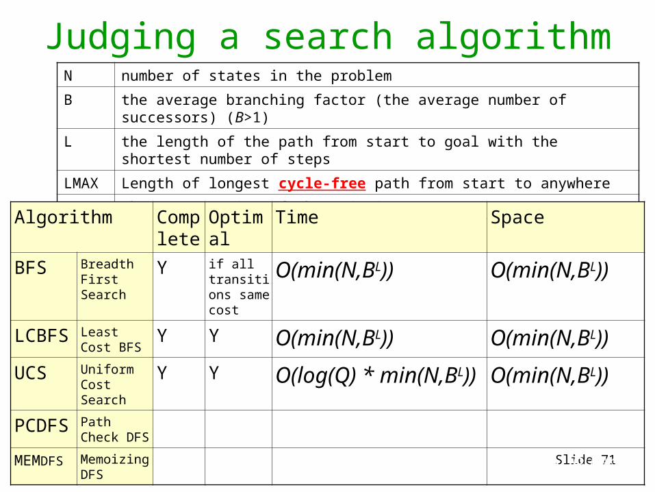
Judging a search algorithmN number of states in the problem
B the average branching factor (the average number of successors) (B>1)
L the length of the path from start to goal with the shortest number of steps
LMAX Length of longest cycle-free path from start to anywhere
Q the average size of the priority queue
Algorithm Complete
Optimal Time Space
BFS Breadth First Search
Y if all transitions same cost
O(min(N,BL)) O(min(N,BL))
LCBFS Least Cost BFS
Y Y O(min(N,BL)) O(min(N,BL))
UCS Uniform Cost Search
Y Y O(log(Q) * min(N,BL)) O(min(N,BL))
PCDFS Path Check DFS
Y N O(BLMAX) O(LMAX)MEMDFS Memoizing
DFSY N O(min(N,BLMAX)) O(min(N,BLMAX))

Slide 72
Judging a search algorithmN number of states in the problem
B the average branching factor (the average number of successors) (B>1)
L the length of the path from start to goal with the shortest number of steps
LMAX Length of longest cycle-free path from start to anywhere
Q the average size of the priority queue
Algorithm Complete
Optimal Time Space
BFS Breadth First Search
Y if all transitions same cost
O(min(N,BL)) O(min(N,BL))
LCBFS Least Cost BFS
Y Y O(min(N,BL)) O(min(N,BL))
UCS Uniform Cost Search
Y Y O(log(Q) * min(N,BL)) O(min(N,BL))
PCDFS Path Check DFS
Y N O(BLMAX) O(LMAX)MEMDFS Memoizing
DFSY N O(min(N,BLMAX)) O(min(N,BLMAX))

Slide 73
Judging a search algorithmN number of states in the problem
B the average branching factor (the average number of successors) (B>1)
L the length of the path from start to goal with the shortest number of steps
LMAX Length of longest cycle-free path from start to anywhere
Q the average size of the priority queue
Algorithm Complete
Optimal Time Space
BFS Breadth First Search
Y if all transitions same cost
O(min(N,BL)) O(min(N,BL))
LCBFS Least Cost BFS
Y Y O(min(N,BL)) O(min(N,BL))
UCS Uniform Cost Search
Y Y O(log(Q) * min(N,BL)) O(min(N,BL))
PCDFS Path Check DFS
Y N O(BLMAX) O(LMAX)MEMDFS Memoizing
DFSY N O(min(N,BLMAX)) O(min(N,BLMAX))

Slide 74
Maze exampleImagine states are cells in a maze, you can move N, E, S, W. What would plain DFS do, assuming it always expanded the E successor first, then N, then W, then S?
G
S
Expansion order E, N, W, S
Other questions:What would BFS do?What would PCDFS do?What would MEMDFS do?

Slide 75
Two other DFS examples
G
S
Order: N, E, S, W?
G
S
Order: N, E, S, W
with loops prevented

Slide 76
Forward DFSearch or Backward DFSearch
If you have a predecessors() function as well as a successors() function you can begin at the goal and depth-first-search backwards until you hit a start.
Why/When might this be a good idea?

Slide 77
Invent An Algorithm Time!
Here’s a way to dramatically decrease costs sometimes. Bidirectional Search. Can you guess what this algorithm is, and why it can be a huge cost-saver?

Slide 78
N number of states in the problem
B the average branching factor (the average number of successors) (B>1)
L the length of the path from start to goal with the shortest number of steps
LMAX Length of longest cycle-free path from start to anywhere
Q the average size of the priority queue
Algorithm Complete
Optimal Time Space
BFS Breadth First Search
Y if all transitions same cost
O(min(N,BL)) O(min(N,BL))
LCBFS Least Cost BFS
Y Y O(min(N,BL)) O(min(N,BL))
UCS Uniform Cost Search
Y Y O(log(Q) * min(N,BL)) O(min(N,BL))
PCDFS Path Check DFS
Y N O(BLMAX) O(LMAX)MEMDFS Memoizing
DFSY N O(min(N,BLMAX)) O(min(N,BLMAX))
BIBFS Bidirection BF Search
Y Y O(min(N,2BL/2)) O(min(N,2BL/2))

Slide 79
N number of states in the problem
B the average branching factor (the average number of successors) (B>1)
L the length of the path from start to goal with the shortest number of steps
LMAX Length of longest cycle-free path from start to anywhere
Q the average size of the priority queue
Algorithm Complete
Optimal Time Space
BFS Breadth First Search
Y if all transitions same cost
O(min(N,BL)) O(min(N,BL))
LCBFS Least Cost BFS
Y Y O(min(N,BL)) O(min(N,BL))
UCS Uniform Cost Search
Y Y O(log(Q) * min(N,BL)) O(min(N,BL))
PCDFS Path Check DFS
Y N O(BLMAX) O(LMAX)MEMDFS Memoizing
DFSY N O(min(N,BLMAX)) O(min(N,BLMAX))
BIBFS Bidirection BF Search
Y All trans same cost O(min(N,2BL/2)) O(min(N,2BL/2))

Slide 80
Iterative DeepeningIterative deepening is a simple algorithm which
uses DFS as a subroutine:
1. Do a DFS which only searches for paths of length 1 or less. (DFS gives up any path of length 2)
2. If “1” failed, do a DFS which only searches paths of length 2 or less.
3. If “2” failed, do a DFS which only searches paths of length 3 or less.
….and so on until success
Cost is
O(b1 + b2 + b3 + b4 … + bL) = O(bL)C
an b
e m
uch
bette
r tha
n re
gula
r
DFS
. Bu
t cos
t can
be
muc
h
grea
ter t
han
the
num
ber o
f sta
tes.
Slide 81
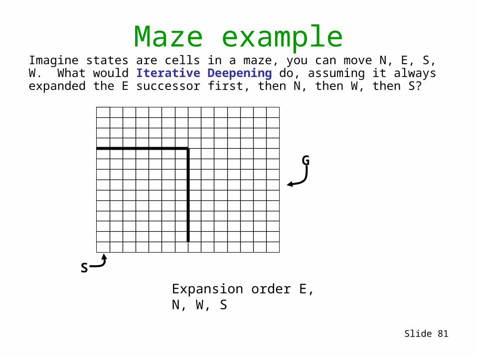
Maze exampleImagine states are cells in a maze, you can move N, E, S, W. What would Iterative Deepening do, assuming it always expanded the E successor first, then N, then W, then S?
G
S
Expansion order E, N, W, S

Slide 82
N number of states in the problem
B the average branching factor (the average number of successors) (B>1)
L the length of the path from start to goal with the shortest number of steps
LMAX Length of longest cycle-free path from start to anywhere
Q the average size of the priority queue
Algorithm Complete
Optimal Time Space
BFS Breadth First Search
Y if all transitions same cost
O(min(N,BL)) O(min(N,BL))
LCBFS Least Cost BFS
Y Y O(min(N,BL)) O(min(N,BL))
UCS Uniform Cost Search
Y Y O(log(Q) * min(N,BL)) O(min(N,BL))
PCDFS Path Check DFS
Y N O(BLMAX) O(LMAX)MEMDFS Memoizing
DFSY N O(min(N,BLMAX)) O(min(N,BLMAX))
BIBFS Bidirection BF Search
Y All trans same cost O(min(N,2BL/2)) O(min(N,2BL/2))
ID Iterative Deepening
Y if all transitions same cost
O(BL) O(L)

Slide 83
N number of states in the problem
B the average branching factor (the average number of successors) (B>1)
L the length of the path from start to goal with the shortest number of steps
LMAX Length of longest cycle-free path from start to anywhere
Q the average size of the priority queue
Algorithm Complete
Optimal Time Space
BFS Breadth First Search
Y if all transitions same cost
O(min(N,BL)) O(min(N,BL))
LCBFS Least Cost BFS
Y Y O(min(N,BL)) O(min(N,BL))
UCS Uniform Cost Search
Y Y O(log(Q) * min(N,BL)) O(min(N,BL))
PCDFS Path Check DFS
Y N O(BLMAX) O(LMAX)MEMDFS Memoizing
DFSY N O(min(N,BLMAX)) O(min(N,BLMAX))
BIBFS Bidirection BF Search
Y All trans same cost O(min(N,2BL/2)) O(min(N,2BL/2))
ID Iterative Deepening
Y if all transitions same cost
O(BL) O(L)

Slide 84
Best First “Greedy” SearchNeeds a heuristic. A heuristic function maps a state onto an estimate of the cost to the goal from that state.
Can you think of examples of heuristics?
E.G. for the 8-puzzle?
E.G. for planning a path through a maze?
Denote the heuristic by a function h(s) from states to a cost value.

Slide 85
Heuristic SearchSuppose in addition to the standard search
specification we also have a heuristic.
A heuristic function maps a state onto an estimate of the cost to the goal from that state.
Can you think of examples of heuristics?
• E.G. for the 8-puzzle?• E.G. for planning a path through a maze?
Denote the heuristic by a function h(s) from states to a cost value.

Slide 86
Euclidian Heuristic
START
GOAL
d
b
pq
c
e
h
a
f
r
2
9 9
81
1
2
3
5
34
4
15
1
25
2
h=12
h=11
h=8
h=8
h=5 h=4
h=6
h=9
h=0
h=4
h=6h=11

Slide 87
Euclidian Heuristic
START
GOAL
d
b
pq
c
e
h
a
f
r
2
9 9
81
1
2
3
5
34
4
15
1
25
2
h=12
h=11
h=8
h=8
h=5 h=4
h=6
h=9
h=0
h=4
h=6h=11
• Another priority queue algorithm.
• But this time, priority is the heuristic
value.

Slide 88
Best First “Greedy” SearchInit-PriQueue(PQ)Insert-PriQueue(PQ,START,h(START))while (PQ is not empty and PQ does not contain a goal state)
(s , h ) := Pop-least(PQ)foreach s’ in succs(s)if s’ is not already in PQ and s’ never previously been visited
Insert-PriQueue(PQ,s’,h(s’))
A few improvements to this algorithm can make things much better. It’s a little thing we like to call: A*….
…to be continued!
Algorithm Complete
Optimal Time Space
BestFS Best First Search
Y N O(min(N,BLMAX)) O(min(N,BLMAX))

Slide 89
What you should know• Thorough understanding of BFS, LCBFS,
UCS. PCDFS, MEMDFS
• Understand the concepts of whether a search is complete, optimal, its time and space complexity
• Understand the ideas behind iterative deepening and bidirectional search
• Be able to discuss at cocktail parties the pros and cons of the above searches