DI

SC

US

SI

ON

P

AP

ER

S

ER

IE

S

Forschungsinstitut zur Zukunft der ArbeitInstitute for the Study of Labor

Slavery, Education, and Inequality

IZA DP No. 5329

November 2010

Graziella BertocchiArcangelo Dimico

Slavery, Education, and Inequality

Graziella Bertocchi University of Modena, CEPR, CHILD and IZA

Arcangelo Dimico

University of Nottingham

Discussion Paper No. 5329 November 2010

IZA

P.O. Box 7240 53072 Bonn

Germany

Phone: +49-228-3894-0 Fax: +49-228-3894-180

E-mail: iza@iza.org

Any opinions expressed here are those of the author(s) and not those of IZA. Research published in this series may include views on policy, but the institute itself takes no institutional policy positions. The Institute for the Study of Labor (IZA) in Bonn is a local and virtual international research center and a place of communication between science, politics and business. IZA is an independent nonprofit organization supported by Deutsche Post Foundation. The center is associated with the University of Bonn and offers a stimulating research environment through its international network, workshops and conferences, data service, project support, research visits and doctoral program. IZA engages in (i) original and internationally competitive research in all fields of labor economics, (ii) development of policy concepts, and (iii) dissemination of research results and concepts to the interested public. IZA Discussion Papers often represent preliminary work and are circulated to encourage discussion. Citation of such a paper should account for its provisional character. A revised version may be available directly from the author.

IZA Discussion Paper No. 5329 November 2010

ABSTRACT

Slavery, Education, and Inequality* We investigate the impact of slavery on the current performances of the US economy. Over a cross section of counties, we find that the legacy of slavery does not affect current income per capita, but does affect current income inequality. In other words, those counties that displayed a higher proportion of slaves are currently not poorer, but more unequal. Moreover, we find that the impact of slavery on current income inequality is determined by racial inequality. We test three alternative channels of transmission between slavery and inequality: a land inequality theory, a racial discrimination theory and a human capital theory. We find support for the third theory, i. e., even after controlling for potential endogeneity, current inequality is primarily influenced by slavery through the unequal educational attainment of blacks and whites. To improve our understanding of the dynamics of racial inequality along the educational dimension, we complete our investigation by analyzing a panel dataset covering the 1940-2000 period at the state level. Consistently with our previous findings, we find that the educational racial gap significantly depends on the initial gap, which was indeed larger in the former slave states.

NON-TECHNICAL SUMMARY

The legacy of slavery for the US economy and society has been the subject of a huge literature. In this paper, we investigate whether it can explain the racial educational gaps which NCLB targets. Our empirical analysis indeed shows that, across the US counties, the current degree of educational inequality, along the racial dimension, can be traced to the intensity of slavery before the Civil War. In other words, those counties that in the past have been more heavily affected by slave labor show a higher degree of racial educational inequality in the present day. Moreover, the data uncover a persistent effect of slavery on the degree of per capita income inequality. On the contrary, the legacy of slavery has no explanatory power for the current level of income per capita. Finally, we show that the driver of income inequality is racial inequality, which is in turn linked to slavery through its impact on the racial gap in education.

JEL Classification: E02, D02, H52, J15, O11 Keywords: slavery, development, inequality, institutions, education

Corresponding author: Graziella Bertocchi Dipartimento di Economia Politica University of Modena Viale Berengario 51 41121 Modena Italy E-mail: graziella.bertocchi@unimore.it

* We would like to thank Daron Acemoglu, Costas Azariadis, Roland Benabou, Raquel Fernandez, Chiara Gigliarano, Oded Galor, Nippe Lagerlöf, Nathan Nunn, Elias Papaioannou, Dietrich Vollrath, as well as participants at the NBER Summer Institute Workshop on Income Distribution and Macroeconomics, the IV Workshop of the Social Choice Research Group, the PRIN Workshop on Political Institutions and Demographic Dynamics, the Rimini Conference in Economics and Finance, and seminars at the Universities of Glasgow and Göteborg, for comments and suggestions. Generous financial support from the Italian University Ministry and Fondazione Cassa Risparmio di Modena is gratefully acknowledged.

2

1. Introduction

Recent developments in growth theory have debated the long-run influence of geography and

institutions on comparative current economic performances. In this paper we address the same issue

within the context of a single country - the United States - where a specific institution - slavery - has

historically been associated more heavily with particular areas - primarily the South. To concentrate

on a single country facilitates the empirical investigation on several grounds, since it reduces the

risk of omitted variable bias that typically plagues across countries investigations. At the same time,

because of their size and history, the US still presents sufficient variations along both the

geographic and the institutional dimensions to make such investigation worthwhile.

In the broader context of the Americas, Engerman and Sokoloff (1997, 2005a) have influentially

argued that factor endowments, in the form of soils, climate, and the size of the native population,

have determined the diffusion of agricultural crops best suited for the employment of slave labor.

The resulting unequal structure of society has in turn contributed to the evolution of a set of legal,

political, and educational institutions meant to preserve the privileges of the elites. Thus, even

though factor endowments themselves can be viewed as exogenous, these initial conditions have

exerted a magnified effect on current performances because the institutions subsequently developed

tended to reinforce their influence. These institutions have then exerted a persistent impact on

economic outcomes long after the abolition of slavery, determining paths of development

characterized by marked inequality in wealth, human capital, and political power. We test this

theory for a cross section of US counties, with special emphasis on the legacy of slavery for the

current level of income and inequality.

Slavery was introduced in North America as early as in the 16th century and its diffusion escalated

throughout the next centuries. Overall, the Middle Passage brought an estimated 645,000 slaves,

mostly from Africa, to the territories that today represent the US. Initially most of the slaves were

settled in the coastal Southern colonies, where they were employed primarily in agriculture. Later,

between the American Revolution and the Civil War, with the Second Middle Passage around a

million slaves were relocated toward the inland regions where the plantation economy was

developing (Berlin, 2003). By the 1860 Census the US slave population had grown to four million,

to represent about 13% of the entire population, distributed within 15 slave states. In the same year,

almost 90% of the blacks living in the US were slaves. After the American Civil War led to the

abolition of slavery in 1865, massive migration flows brought the former slaves from the rural

South to the urban North. By 1940 75% of black men still lived in the South. By 2000, the fraction

3

had further declined to about 55%. Therefore, the majority of the blacks are still located in the

South, while for white men the corresponding fractions are much smaller at about 28% and 16%,

respectively. In fact, the cross state correlation between the fraction of slaves in the population in

1860 and the fraction of blacks in 2000 is 0.80. These figures indicate that, throughout American

history and even after the end of the institution of slavery, the economic welfare of blacks has been

tied closely to the performance of the Southern economy (Smith and Welch, 1989).

The historiography of slavery in America is huge. Economic historians have focused on the

profitability and the efficiency of slavery. In their provocative and controversial empirical work on

the antebellum South, Fogel and Engerman (1974) suggested that slavery was both productive and

economically efficient, a conclusion which was criticized, among others, by David et al. (1976).

Lagerlöf (2009) and Acemoglu and Wolitzky (2010) model the economics of labor coercion from a

related perspective. A parallel research effort has been devoted to the long-term legacy of slavery,

in a number of dimensions. While Nunn (2008a) has focused on the implications of slave trades in

Africa, Engerman and Sokoloff (2005a) and Nunn (2008b) have examined the impact of slavery in

the receiving countries. In particular, on the basis of historical evidence, the former formulate the

hypothesis that factor endowments, through large-plantation slavery and other inequality-

perpetuating institutions, may have hampered subsequent economic growth. The latter estimates

the influence of slavery on the current performances of the US economy, to find that slave use is

negatively correlated with subsequent economic development, but that this relationship is not

driven by large-scale plantation slavery, i.e., a more precise measure of factor endowments. He also

finds a positive impact of slavery on 1860 land inequality, which is in turn correlated with current

income inequality, but no impact of 1860 land inequality on current income, which suggests that

inequality may not be the channel of influence running from factor endowments to the current level

of development. Mitchener and McLean (2003) find that the legacy of slavery has a strong and

persistent effect on productivity levels across US states in the 1880-1980 period. Lagerlöf (2005)

explores the link between geography and slavery and also documents a negative relationship

between slavery and current income. A common conclusion for this stream of the literature is a

negative relationship between past slavery and current income per capita across US states and

counties, even though the channels through with this influence materializes are still unclear.

A separate research line has focused on the impact of race on inequality. This work has documented

that, since emancipation and especially since 1940, the average income of black Americans has

increased greatly, both in absolute and relative terms. The determinants of the relative improvement

of the economic status of blacks after WWII, however, have been the subject of debate. Both the

4

civil rights movement, with its impact on the labor market through affirmative action laws, and

long-term changes in human capital have been advanced as possible explanations of the observed

trend (Heckman, 1990 and Margo, 1990). The main contributions to the line of research on race and

human capital are Smith (1984), Smith and Welch (1989), followed by Margo (1990) and Collins

and Margo (2006).1 The evidence collected by these authors documents the evolution of racial

differences both in the quality and the quantity of education, starting from the emancipation of

blacks in the post-Civil War era and taking into account the potential legacy of slavery for human

capital accumulation. Initially African-Americans had essentially no exposure to formal schooling,

as a legacy of the extremely high rates of illiteracy that existed under slavery. The first generations

of former slaves were able to complete far fewer years of schooling, on average, than whites.

Moreover, they had access to racially segregated public schools, mostly in the South, where they

received a qualitatively inferior education, even if compared to that received by Southern whites.2

In an initial phase, the combination of low educational attainment and inferior educational quality

determined the persistence of large wage and income gaps. Subsequently, however, the racial

schooling gap declined, as successive generations of black children received more and better

schooling, with an eventual impact on earnings. Overall, despite the initial conditions and the

persistence of discrimination, the reported evidence on the evolution of educational differences, in a

wide number of dimensions (such as literacy rates, years of educational attainment, spending per

pupil, and returns to literacy), overwhelmingly points to long-term convergence. A related stream of

the literature on racial inequality in education has measured the long-term influence of family

background (as captured by ability, or parental education) on the schooling process (see for example

Cameron and Heckman, 2001). Within this stream, Sacerdote (2005) has focused on a comparison

between the grandchildren of former slaves and free blacks, to find substantial convergence of

educational outcomes, since by 1920 the remaining legacy of slavery is such that all blacks are

affected equally. While the contribution of human capital to the improvement of the economic status

of blacks cannot be disputed, as previously mentioned other factors have also been evaluated. In

particular, it has been argued that at the beginning of the 20th century employment segregation in

agriculture, especially in the South, was also instrumental in delaying income convergence, while

after WWI an increased demand of black labor in the North may have accelerated it. Likewise,

further pressure toward convergence occurred in the 1960s with the civil rights movement.

Given these premises, to investigate the long-term impact of slavery on current economic

performances, we start by revisiting the available evidence on the impact of slavery on current per 1 See also Goldin and Margo (1992), Goldin (1998), and Goldin and Katz (1999). 2 Naidu (2010) estimates the effect of the 19th century disenfranchisement laws for blacks in the South and finds that they are associated with a fall in black educational inputs and thus with low-quality Southern schooling.

5

capita income. We find that, contrary to what previously established in the above cited literature,

there is no robust evidence that those US counties that employed slave labor more heavily are

poorer today than those that did not. Next we turn to examine how the current level of inequality is

shaped by slavery. We find that the distribution of per capita income is more unequal today in

former slave counties. These results taken together indicate that the long-term influence of slavery

on per capita income is not on its level, but on its distribution within each county. Moreover, we

identify the driver of income inequality in racial inequality, which is in turn determined by slavery.

To test the channels through which slavery determines current income inequality, we compare three

alternative theories: a land inequality theory, a racial discrimination theory, and a human capital

transmission theory. To be noticed is that, at least in principle, the three channels are not mutually

exclusive since, as suggested by Sokoloff and Engerman (2000) and Acemoglu et al. (2008),

institutional and economic development paths may be interlinked and jointly determined by various

factors. For instance, the institution of public schooling, which has been a major vehicle of capital

accumulation, as well as the removal of de facto and de jure discrimination, may have been more

rapid and more effective in the same counties where factor endowments prevented the diffusion of

slavery. The empirical evidence previously reviewed on race and inequality also points to complex

connections among all these aspects.

Once again, the land inequality theory derives from the Engerman and Sokoloff hypothesis that

links factor endowments to institutions and economic performances. If this theory is verified, the

legal institution of slavery would affect current performances through its link with factor

endowments. In our context, the latter could be measured by land inequality, which should in turn

reflect the diffusion of those crops that were typical of large-scale plantations and thus of the use of

slave labor.

Our second test evaluates the potential explanatory power of those racial discrimination theories

which have emphasized racial differences in the value of skills. Racial discrimination can manifest

itself on the schooling dimension, through a worse quantity and quality of the education publicly

provided, or directly on the labor market, by denying blacks access to certain jobs (see Smith,

1984). To measure the impact of these aspects on racial inequality and to verify its connection with

the legacy of slavery, we construct a measure of racial discrimination by comparing the returns on

education for blacks and whites.

Our third channel of influence is represented by human capital transmission. The hypothesis we test

6

is that the long-term influence of slavery may run through its negative impact on human capital

accumulation. According to this hypothesis, which is closely associated with Smith (1984) and the

above-mentioned work on race and human capital, the counties more affected by slavery should be

associated with worse educational attainment for the black population.

For a cross section of counties, our empirical investigation supports the third theory, i. e., even after

controlling for potential endogeneity, we find that current income inequality is primarily influenced

by slavery through the impact exerted by the latter on the unequal educational attainment of blacks

and whites. If we compare our results with the Engerman and Sokoloff hypothesis, we can

conclude that indeed the presence of an association among factor endowments, institutions and

inequality is confirmed, but also that the final link between these variables and economic

development is missing in our findings. In particular, the institution of slavery does not affect the

current level of development, possibly because the potential variations in this dimension are

absorbed by a number of national factors that attenuate it. Moreover, while factor endowments, as

measured by land inequality, do exert a direct effect on current inequality, their impact does not run

through the specific institution we focus on, i.e., slavery, even though we cannot rule their potential

impact on other relevant institutions we do not consider (e.g., political institutions).

To improve our understanding of the dynamics of racial inequality along the educational dimension,

we complete our investigation by analyzing a panel dataset covering the 1940-2000 period at the

state level. We find that the racial educational gap significantly depends on the initial gap. Since the

initial gap was larger in the former slave states, this confirms the influence of slavery on racial

educational inequality.

The rest of the paper is organized as follows. In Section 2 we revisit the evidence on the impact of

slavery on the current level of development. In Section 3 we examine its impact on the current level

of inequality. In Section 4 we explore three alternative channels through which this impact

materializes. In Section 5 we review our results in Section 4 to control for endogeneity. In Section 6

we complete our investigation by analyzing the evolution of educational attainment in the 1940-

2000 period. In Section 7 we derive our conclusions.

2. Slavery and Development: Revisiting the Evidence

As mentioned in the introduction, it has been argued that slavery in the US has had a negative and

significant effect on current per capita income. However, the channels through which slavery should

7

affect current development have not been clarified. In more detail, Nunn (2008b) employs data at

the county level to test the Engerman and Sokoloff hypothesis and finds that slave use is negatively

correlated with subsequent economic development, but that this relationship is not driven by large-

scale plantation slavery, as suggested by the above hypothesis. He also finds a positive impact of

slavery on inequality, for a measure of inequality given by the Gini coefficient of land holdings in

1860, which appears positively correlated with 2000 income inequality. However, he finds no

impact of the 1860 land Gini on 2000 income. Lagerlöf (2005) also finds a negative relationship

between slavery and current income at the county level, but he limits his investigation to the

counties belonging to former slave states. Finally, on the basis of state level data, Mitchener and

McLean (2003) argue that slavery has affected productivity as measured by income per worker.

Given the state of art, we start by re-investigating the long-run effects of slavery and then we try to

shed light on the mechanism at work.

In Figures 1 and 2 we plot income per capita in 2000 on the share of slaves to the total population in

1860.3 Figure 1, which includes all counties, shows a negative and significant relationship between

slavery and income per capita but, when in Figure 2 we confine the plot to counties within former

slave states, the relationship becomes not significant. The plots therefore suggest that the results

from the literature previously reviewed may not be robust, so that they may not actually capture a

causal effect of slavery. The fact that the partial correlation turns to be insignificant (and of opposite

sign) once confined to the sub-sample of slave states may indicate that the negative effect of slavery

on development only captures simple structural differences between the North and the South of the

US, or between slave states and non-slave states.

3 See the Data Appendix for data sources.

8

Figure 1: Slavery and Income per Capita (All Counties)

Figure 2: Slavery and Income per Capita (Only Counties in Slave States)

In order to investigate this hypothesis, in Table 1 we first re-estimate the same model as in Nunn

(2008b) and then we enter geographical controls which should capture structural differences among

different regions of the US. More specifically, we control for counties within former slave states and

for counties within North Eastern and South Atlantic states. The last two controls are necessary

because there is evidence that states in these regions have a higher income per capita (see Rappaport

and Sachs, 2003 and Lagerlöf, 2005). Model 1 replicates the basic model in Nunn (2008b), where

population density in 1860 is also entered as a proxy for initial prosperity (as in Acemoglu et al.,

2002). As expected we find a negative and significant effect of slavery on current income per capita.

ALAL

ALAL

ALAL

AL ALAL AL

ALAL

ALALALAL ALALAL AL

AL

ALAL

AL

AL ALAL

ALAL

AL

ALAL AL

ALAL

ALAL

ALAL

ALAL

ALAL

AL

ALAL

ALAL

ALAL

ALAL

AR ARAR

ARARAR ARAR

ARARARAR

ARARARAR

ARAR

AR ARAR

AR

ARAR AR

AR ARARARARARARAR

AR

AR

AR ARAR ARAR

ARAR

AR

AR AR

ARAR

AR

AR

AR

AR

AR

ARARAR

CA

CACACACA

CA

CA

CA

CACA

CA

CA

CACA

CA

CA

CA

CA

CA

CACA

CA

CA

CA

CACA

CA

CA

CA

CA

CACACA

CA

CA

CACA

CACACACA

CA

CA

CO

CT

CTCTCTCTCTCTCTDE

DE

DEFL

FL

FL

FL

FL

FL

FL

FLFL FL

FL

FLFL

FLFL

FL

FL

FL

FLFL

FL

FL

FL

FL

FLFL

FL

FL

FL

FL

FLFLFL FL

FL FLGA GAGA

GA

GA

GA

GA

GA

GA

GA GAGA

GAGA

GAGA

GA

GAGA

GA

GA

GA

GAGA

GA

GA

GAGA

GAGA

GAGA

GA

GA

GA

GA

GAGA

GA

GAGA

GAGA

GA

GA

GA

GA

GA

GAGA

GA

GA GA

GA

GAGA

GA

GA

GA

GA

GA

GA GA

GAGA

GAGA

GAGAGA

GA

GAGAGA

GAGA

GA

GA

GAGAGA GA

GA

GA

GA

GAGA

GAGA

GAGA GAGA GA GA

GA

GAGA

GAGA

GA

GAGAGA

GAGA

GA GAGA GA

GAGA

GA

GA

GA GAGA GAGAGA

GAGA GA

GA

GA

GA

GAGAGA

IL

ILIL

IL

IL

ILILILILILILILILILIL

IL

ILILILILIL

IL

ILIL

IL

IL

IL

ILILILIL

IL

IL

IL

ILILILILILILILIL

IL

IL

IL

IL

IL

IL

IL

ILILILILILIL

ILILILILILILILILIL

ILILIL

ILILILILIL

IL

IL

ILILIL

IL

ILILILIL

IL

IL

ILILILILILIL

ILILILIL

IL

ILILILILILILILIN

ININ

ININ

ININ

INININ

ININININ

ININININ

INININ

IN

ININININININ

IN

IN

IN

IN

ININININININININ

IN

ININ

IN

ININININ

IN

ININININININ

ININININININININ

ININ

INININININ

IN

IN

ININ

IN

IN

ININ

ININ

IN

IN

ININININ

IN

INININININIAIAIAIAIAIAIAIAIAIAIAIAIAIAIAIAIAIAIAIA

IAIAIAIA

IA

IAIA

IAIAIAIAIAIAIAIAIAIA

IAIAIAIAIAIAIAIAIAIA

IA

IA

IAIAIA

IAIAIAIA

IA

IAIAIAIAIAIAIAIAIAIAIAIAIAIAIAIAIA

IA

IAIA

IAIA

IA

IAIAIAIAIAIAIAIAIAIA

IA

IAIAIAIAIA

IA

KSKSKSKSKSKSKS

KSKSKSKSKSKSKSKSKSKS

KS

KS

KSKS

KSKSKSKSKSKSKSKSKS

KSKSKSKSKS

KYKY

KYKYKY

KY

KY KYKY KY

KYKY

KY

KY

KY

KYKYKYKY

KYKY

KY

KY

KY

KY KYKY

KY

KYKY

KY

KYKY

KY

KY

KY KYKYKY

KYKY

KY

KYKY

KY

KY

KY

KYKY

KY

KY

KY

KY

KY

KY

KY

KY

KYKY

KYKY

KY

KY

KYKY

KY

KYKY

KY

KY

KYKY KYKY

KY

KYKY

KY

KY

KYKY

KYKY

KY

KYKY

KYKYKY

KY

KY

KYKYKY

KYKY

KY

KYKY KYKY

KY

KYKY

KY

KY

KY

KY

KY

LA

LALALA

LALALA

LA LALA LALA

LA

LALA

LALA

LA LA

LALA

LA

LALA

LALALA LALA

LA

LA

LA

LALALA

LA LA

LA

LA

LALALA

LA LA

LA

LALA

MEME

ME

ME

MEMEMEME

MEME

ME

ME

MEMEME

MEMD

MDMDMD

MD

MDMD

MD

MD

MDMD

MD

MD

MD

MDMD MD

MD

MD

MD MDMD

MA

MAMAMAMA

MAMAMA

MAMAMA

MA

MA

MA

MI

MIMIMIMIMIMIMIMIMIMIMI

MIMIMIMIMI

MI

MI

MIMIMI

MIMI

MIMIMIMIMIMIMIMIMI

MI

MI

MI

MIMIMI

MI

MIMI

MI

MI

MI

MI

MIMIMI

MI

MI

MIMIMIMIMIMIMIMI

MI

MI

MN

MN

MNMNMNMNMN

MN

MN

MNMNMN

MN

MNMNMNMNMN

MN

MN

MNMNMNMN

MN

MNMNMNMNMNMNMNMNMN

MNMNMNMN

MN

MNMN

MNMN

MN

MNMNMN

MN

MNMNMNMN

MN

MNMN

MN

MNMNMN

MS

MSMS MSMS

MSMSMS MS

MSMS

MSMS

MS

MSMS

MSMS MS

MS

MS

MSMS

MS

MS

MS

MSMS

MS

MSMSMS

MS

MS MSMSMS MS

MSMS

MSMS

MSMS

MS

MSMSMS

MSMS

MSMS MS

MS

MSMS

MS

MS MS MSMO

MOMO

MOMOMO MO

MOMO

MOMOMO

MOMO

MOMO

MO

MO

MO

MO

MOMOMO

MOMO

MO

MOMOMOMO

MO

MO

MO

MO

MO

MOMOMO

MO

MOMO MO

MO

MOMOMO MO

MO

MOMOMOMOMO

MO

MO MO

MOMOMO

MO

MOMOMO

MOMO

MOMOMO MOMO

MOMOMOMO

MO

MO

MO

MOMO MOMO

MO

MO

MO

MO

MO

MOMOMO

MOMO

MO

MO

MOMO

MO

MO

MO

MO MO

MO

MOMOMOMOMO

MO

MO

MO

MOMOMOMO

NENENE

NENENE

NE

NENENENE

NE

NENE

NE

NE

NE

NE

NE

NE

NENENENENENE

NENENV

NVNHNHNHNH

NHNHNHNH

NHNHNJ

NJ

NJNJNJ

NJ

NJ

NJNJ

NJ

NJNJNJ

NJ

NJNJNJ

NJ

NJNJ

NJNM

NM

NM

NM

NM

NMNMNM

NY

NY

NY

NYNYNYNYNYNY

NY

NYNY

NYNY

NYNY

NYNYNYNYNYNYNY

NY

NYNY

NY

NY

NY

NYNYNYNYNY

NYNYNY

NY

NYNYNY

NY

NY

NYNY

NYNYNY

NY

NY

NYNYNYNYNY

NY

NY

NY

NYNY

NCNCNC

NCNC NC NCNCNC

NC

NC

NCNC

NCNC

NC

NCNC

NC

NCNC NCNCNCNCNC

NC

NC NC

NC

NCNC

NCNCNC

NC

NCNCNC

NC

NCNC

NC

NCNC

NCNC

NCNCNC

NC NC

NC

NC

NCNC NC

NCNC

NC

NCNC

NCNC

NC

NCNC

NC

NCNCNC NC

NC NCNC

NC

NC

NC

NCNC

NCNC

NC NCNCNCOH

OHOHOH

OH

OH

OHOH

OH

OHOHOHOHOH

OHOHOH

OH

OHOH

OH

OHOH

OH

OHOH

OH

OH

OH

OH

OHOH

OHOH

OH

OHOHOH

OH

OHOHOH

OH

OH

OHOHOHOHOHOHOH

OH

OH

OHOH

OH

OH

OHOHOH

OH

OH

OH

OH

OHOH

OHOHOHOHOHOHOHOHOHOHOHOHOHOHOH

OH

OH

OHOHOHOHOH

OROR

OROROROROROROR

OROROR

OR

OROROR

OR

ORP A

P A

P AP A

P A

P AP AP A

P A

P AP AP AP A

P A

P AP AP AP AP A

P AP AP A

P AP AP AP A

P AP AP AP A

P AP AP A

P A

P AP AP A

P AP AP AP AP AP A

P A

P AP A

P AP AP A

P AP AP A

P A

P AP AP AP AP AP AP AP A

P A

P AP AP A

RIRIRI

RI

RI

SCSC

SC

SCSC

SCSCSC SC

SC

SC

SCSC

SC

SCSCSC SC

SC

SC SC

SCSCSC

SCSC

SCSCSC

SCT N

T NT NT N

T NT N

T N

T N T NT N

T N

T NT N

T NT N

T N

T NT N

T NT N T N

T NT NT N T N

T N

T N

T N

T N

T NT N

T NT N T N

T N T N

T NT NT NT N

T N

T N

T N

T NT N

T NT NT NT N

T NT N

T N T N

T NT N

T N

T N

T N

T NT N

T N

T N

T NT N

T N T N

T NT N

T N

T N

T NT N

T N T N

T N

T NT N

T NT N

T N

T NT N

T N

T N

T X

T X

T X

T XT XT X

T X

T XT XT X

T X T XT X

T XT XT X

T XT X

T X

T X

T XT X

T XT X

T X

T X

T X

T XT X

T X

T XT X

T XT X

T X

T XT X

T XT X

T X

T X

T X

T X

T XT X

T X

T XT X

T X

T XT X T X

T X

T XT XT X

T X

T XT X T XT X

T X

T XT X

T XT X

T X

T XT X

T X

T X

T X

T XT X

T XT XT X

T X T XT X

T XT X

T X

T X

T XT XT X

T X

T XT X

T X

T X T XT X T X

T X T X

T X

T X

T X

T XT XT X

T XT XT X

T XT X

T X

T X

T X

T X

T X T X

T X

T XT XT XT X

T X

T X

T X

T X

T X

T X

T X

T X

T X

T X

T XT X

UTUTUT

UT

UTUTUT

UT

UT

UTUTUT

UTVTVT

VT

VT

VT

VT

VTVTVTVTVTVTVTVT

VAVA

VAVA

VA

VAVA

VAVA

VA

VAVA

VA

VA VA

VA

VA

VAVA

VA

VA

VAVAVA

VA

VA

VAVA VA

VAVA

VAVA

VA

VAVA

VA

VA

VA

VA

VA

VA

VA

VA

VAVA

VA

VAVA

VAVA

VAVA

VA

VA

VA

VA

VAVAVA

VAVA

VA

VA VAVA

VAVA

VAW AW A

W AW AW A

W A

W AW AW A

W AW AW AW A

W AW AW A

W IW IW IW I

W I

W I

W I

W IW I

W I

W I

W I

W I

W I

W I

W IW IW IW I

W IW IW IW IW I

W I

W I

W I

W I

W I

W I

W IW I

W I

W I

W IW I

W I

W I

W I

W IW IW I

W I

W I

W I

W I

W I

W I

W I

W I

W I

W I

W I

W I

W I

W I

W IW I

Y=10.0678 - 0.2431(-10.76) X

99.

510

10.5

1111

.5

0 .2 .4 .6 .8 1slave_1860

lnincome_00 Fitted values

Y= 9.940 + 0.036 (1.14) X

99.

510

10.5

11

0 .2 .4 .6 .8 1slave_1860

lnincome_00 Fitted values

9

In Model 2 we enter the slave states dummy together with our two geographical dummies and the

effect of slavery becomes insignificant, while the coefficients of the dummies are significant and

with the expected sign. In Model 3 we replace the slave states dummy with a dummy for Southern

states,4 and the slavery variable is again not significant. In Model 4 and 5 we confine the estimates

respectively to slave states and Southern states: in these additional models the dummy for Atlantic

states is the only variable which retains a significant effect. To sum up, the results from Table 1

show that the negative effect of slavery which was found in related papers captures structural

differences among US regions and, in particular, between former slave and non-slave states, or

between South and North. Once we control for these structural differences, there is not any

significant direct effect of slavery on current income per capita.5

Table 1: Slavery and Economic Development

Dependent Variable: Per Capita Income 2000 Estimation Method: OLS Model 1 Model 2 Model 3 Model 4 Model 5 Slaves/Population 1860 -0.239*** -0.0249 -0.0497 -0.0211 -0.0287 (-10.99) (-0.79) (-1.51) (-0.67) (-0.85) Population Density 1860 0.0444*** 0.0386*** 0.0387*** 0.297 0.263 (7.26) (9.37) (9.22) (1.59) (1.61) North East Dummy 0.0982*** 0.120*** (5.61) (6.89) South Atlantic Dummy 0.107*** 0.111*** 0.103*** 0.107*** (7.57) (7.79) (7.40) (7.55) Slave States Dummy -0.174*** (-13.64) South Dummy -0.148*** (-10.53) Constant 10.06*** 10.09*** 10.07*** 9.911*** 9.911*** (1652.16) (1464.86) (1515.65) (886.96) (753.30) Observations 1960 1960 1960 1026 913 R-squared 0.08 0.21 0.18 0.08 0.08 Sample All Counties All Counties All Counties Slave States South States *** p<0.01, ** p<0.05, * p<0.1. Robust t statistics in parentheses.

After establishing that the effect of slavery on current economic performances (as of the year 2000)

is absent, we also test whether this conclusion holds in previous decades. In Table 2, we re-estimate

the complete model (Model 2) in Table 1 for income per capita in 1990, 1980 and 1970 and we find

that the effect of slavery on income per capita has faded at least since 1980. There is a moderate and

4 The correlation between the two dummies is high but not perfect, at 0.83. 5 For the state of São Paulo (Brazil), Summerhill (2010) also finds that the intensity of slavery in 1872 has no discernable negative impact on income in 2000.

10

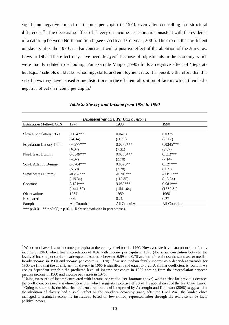
significant negative impact on income per capita in 1970, even after controlling for structural

differences.6 The decreasing effect of slavery on income per capita is consistent with the evidence

of a catch-up between North and South (see Caselli and Coleman, 2001). The drop in the coefficient

on slavery after the 1970s is also consistent with a positive effect of the abolition of the Jim Craw

Laws in 1965. This effect may have been delayed7 because of adjustments in the economy which

were mainly related to schooling. For example Margo (1990) finds a negative effect of ‘Separate

but Equal’ schools on blacks' schooling, skills, and employment rate. It is possible therefore that this

set of laws may have caused some distortions in the efficient allocation of factors which then had a

negative effect on income per capita.8

Table 2: Slavery and Income from 1970 to 1990

Dependent Variable: Per Capita Income Estimation Method: OLS 1970 1980 1990 Slaves/Population 1860 0.134*** 0.0418 0.0335 (-4.34) (-1.25) (-1.12) Population Density 1860 0.0277*** 0.0237*** 0.0345*** (6.07) (7.31) (8.67) North East Dummy 0.0549*** 0.0366*** 0.112*** (4.37) (2.78) (7.14) South Atlantic Dummy 0.0764*** 0.0323** 0.127*** (5.60) (2.28) (9.69) Slave States Dummy -0.252*** -0.201*** -0.192*** (-19.34) (-15.85) (-15.54) Constant 8.181*** 9.080*** 9.681*** (1441.89) (1541.64) (1632.81) Observations 1959 1959 1960 R-squared 0.39 0.26 0.27 Sample All Counties All Counties All Counties *** p<0.01, ** p<0.05, * p<0.1. Robust t statistics in parentheses.

6 We do not have data on income per capita at the county level for the 1960. However, we have data on median family income in 1960, which has a correlation of 0.82 with income per capita in 1970 (the serial correlation between the levels of income per capita in subsequent decades is between 0.89 and 0.79 and therefore almost the same as for median family income in 1960 and income per capita in 1970). If we use median family income as a dependent variable for 1960 we find that the coefficient for slavery in 1960 is significant and equal to 0.23. A similar coefficient is found if we use as dependent variable the predicted level of income per capita in 1960 coming from the interpolation between median income in 1960 and income per capita in 1970. 7 Using measures of income correlated with income per capita (see footnote above) we find that for previous decades the coefficient on slavery is almost constant, which suggests a positive effect of the abolishment of the Jim Crow Laws. 8 Going further back, the historical evidence reported and interpreted by Acemoglu and Robinson (2008) suggests that the abolition of slavery had a small effect on the Southern economy since, after the Civil War, the landed elites managed to maintain economic institutions based on low-skilled, repressed labor through the exercise of de facto political power.

11

3. Slavery and Inequality: New Evidence

According to the Engerman and Sokoloff hypothesis, the initial presence of specific factor

endowments explains the development of agricultural production techniques based on slave labor,

which in turn resulted in extreme economic inequality and in a set of political (Engerman and

Sokoloff, 2005b), redistributive (Sokoloff and Zolt, 2007), and educational (Mariscal and Sokoloff,

2000) institutions that reflected this inequality. The link between factor endowments and inequality

is also empirically documented. Galor et al. (2009) find evidence that land inequality adversely

affected the emergence of human capital promoting institutions, as measured by educational

expenditure across US states in the 1900-1940 period. Vollrath (2010) finds evidence of a negative

effect of inequality on property tax revenues in 1890. Ramcharan (2009) tests the relationship

between land inequality and redistribution and finds a significant effect of land inequality on

redistributive policies in the 1890-1930 period. Over a cross section of slave counties, Lagerlöf

(2005) finds that counties which in 1850 had a larger slave population display higher racial

inequality today. However, the link between slavery and overall economic and racial inequality

today still remains unclear. The channel through which this link may have worked is also poorly

understood.

In Table 3 we show the distribution of inequality and poverty across the nine US Census regions.

The three Southern regions, where the share of slaves was the largest, are the ones with highest

levels of inequality (both in terms of racial and income inequality). The share of the population

below the poverty level is also highest in the three Southern regions. However the table only

provides some statistical association between variables which of course can depend on structural

differences between regions as for the case of income per capita. For example, most of the Southern

states (e.g., Texas, Louisiana, Kansas, etc.) are rich in natural resources (mainly oil) which may

explain a higher degree of inequality through a resource curse.

In Table 4 we test the relationship between slavery and current economic inequality once we control

for structural differences which we proxy with appropriate dummies as in Table 1. In Model 1 we

regress income inequality9 on slavery, controlling for the same set of dummies introduced in Model

2 of Table 1, i.e., the slave states dummy and two geographical dummies. As in Table 1, we also

enter population density as a control for initial differences in income across counties. We find that

slavery has a positive and significant effect on income inequality, even under our controls. The

dummy for slave states is also positive and significant suggesting that, beside slavery, there may be

9 See the Data Appendix for an explanation of the method used to calculate income inequality at the county level.

12

other reasons that have worsened current economic inequality within these states. The dummy for

the North East is also associated with higher inequality, even if the size of the coefficient is small,

while South Atlantic states display less inequality. In Model 2 we replace the slave states dummy

with the South dummy, to obtain very similar results. In Model 3 we confine the estimates to slave

states only. In all specifications, slavery always retains a positive and significant coefficient.

Table 3: Descriptive Statistics

Table 4: Slavery and Economic Inequality

Dependent Variable: Income Inequality

Estimation Method: OLS Model 1 Model 2 Model 3 Slaves/Population 1860 0.0374*** 0.0331*** 0.0375*** (7.42) (6.39) (7.46) Population Density 1860 0.00304*** 0.00302*** 0.0117 (4.28) (4.36) (0.86) North East Dummy 0.0108*** 0.00817*** (6.25) (4.78) South Atlantic Dummy -0.0212*** -0.0240*** -0.0214*** (-9.58) (-10.73) (-9.60) Slave States Dummy 0.0335*** (17.64) South Dummy 0.0353*** (17.34) Constant 0.387*** 0.390*** 0.420*** (409.51) (421.94) (251.81) Observations 1984 1984 1050 R-squared 0.31 0.31 0.11 Sample All Counties All Counties Slave States *** p<0.01, ** p<0.05, * p<0.1.Robust t statistics in parentheses.

Region Freq. Slaves Inc. Wht Inc. Blk Racial Ineq Income Ineq Share Blk Share Wht Poverty

New England 67 0 22873 15280 0.031 0.392 2.013 92.149 0.088Middle Atlantic 150 0.0004 21668 13508 0.044 0.399 5.354 87.047 0.102East North C. 437 0 19449 13383 0.027 0.386 3.109 92.396 0.097West North C. 617 2.83 17546 12472 0.030 0.398 1.186 92.295 0.110South Atlantic 584 36.70 20321 13078 0.084 0.417 21.06 73.381 0.143East South C. 364 28.26 17341 11244 0.065 0.436 17.13 80.082 0.169West South C. 469 29.10 18731 10713 0.110 0.432 10.82 68.905 0.178Pacific 278 0.0213 19080 13577 0.068 0.405 7.13 79.929 0.139Mountain 153 0 23317 17408 0.102 0.405 1.758 71.981 0.134

Total 3119 15.62 19219 12748 0.063 0.410 8.693 81.470 0.135

13

In Table 5 we focus on racial inequality (measured by horizontal income inequality)10. and the effect

of slavery is even more significant.11 In Model 1 the dummy for slave states is significant but turns

to be negative while the dummies for Southern and North Eastern counties are respectively

insignificant and marginally significant. In Model 2 we replace the slave states dummy with the

South dummy and then in Model 3 we restrict the estimates to former slave states only. Results for

both models are similar to those from Model 1. We therefore can conclude that there is a robust

relationship between slavery and current income and racial inequality.

Table 5: Slavery and Racial Inequality

Dependent Variable: Racial Inequality

Estimation Method: OLS Model 1 Model 2 Model 3 Slaves/Population 1860 0.178*** 0.162*** 0.179*** (26.33) (22.15) (26.70) Population Density 1860 0.0102*** 0.0102*** 0.0532*** (5.83) (5.84) (2.83) North East Dummy 0.00126 0.00475 (0.41) (1.57) South Atlantic Dummy -0.00537* -0.00842*** -0.00597* (-1.75) (-2.63) (-1.95) Slave States Dummy -0.00647** (-2.16) South Dummy 0.00590* (1.71) Constant 0.0355*** 0.0320*** 0.0279*** (23.39) (23.21) (10.84) Observations 1984 1984 1050 R-squared 0.40 0.40 0.40 Sample All Counties All Counties Slave States *** p<0.01, ** p<0.05, * p<0.1. Robust t statistics in parentheses.

Next in Table 6 we estimate the effect of slavery on the share of the population below the poverty

level. As in previous tables in Model 1 we control for former slave states. In Model 2 we replace the

slave states dummy with the South dummy. Finally in Model 3 we restrict the estimates to counties

in former slave states only. The effect of slavery on the share of the population below poverty is

significant and positive under all specifications. It is therefore obvious to infer that slavery affects

the poverty rate (which is likely to be more prevalent among blacks) which in turn contributes to the

level of racial and income inequality within the country.

10 See Data Appendix. 11 Consistently, in Lagerlöf (2005) slavery increases white income and decreases black income.

14

Table 6: Slavery and Poverty

Dependent Variable: Population Below Poverty Level Estimation Method: OLS Model 1 Model 2 Model 3 Slaves/Population 1860 0.0575*** 0.0520*** 0.0575*** (6.40) (5.54) (6.42) Population Density 1860 0.00377*** 0.00374*** 0.00768 (4.93) (5.04) (0.22) North East Dummy -0.00109 -0.00534** (-0.45) (-2.19) South Atlantic Dummy -0.0357*** -0.0397*** -0.0357*** (-10.42) (-11.29) (-10.42) Slave States Dummy 0.0523*** (15.43) South Dummy 0.0540*** (14.07) Constant 0.0972*** 0.101*** 0.149*** (74.68) (77.46) (46.65) Observations 1984 1984 1050 R-squared 0.32 0.32 0.11 Sample All Counties All Counties Slave States *** p<0.01, ** p<0.05, * p<0.1. Robust t statistics in parentheses.

Finally in Table 7 we test whether slavery affects racial inequality through income disparities, or

vice versa. In order to test these alternative hypotheses we first enter income inequality as an

additional regressor in the model in which we regress racial inequality on slavery (Model 1). In the

second model (Model 2) we enter racial inequality as a regressor for economic inequality. In both

cases, we also control for population density and for the set of dummies that appear in the first

specifications of Tables 4-6- In Model 1, income inequality hardly diminishes the effect of slavery

on racial inequality. There is a positive effect of income inequality on racial inequality, but it is hard

to establish a causality given that the two variables are for the same year. In Model 2, once we

control for racial inequality, slavery is no longer significant in a regression for economic inequality.

Therefore, our results suggest that the impact of slavery on economic inequality runs through its

impact on racial inequality. In the next two models (Models 3 and 4) we replicate the same test for

the share of population below the poverty level. Consistently we again find that the effect of slavery

on poverty runs through racial inequality.

15

Table 7: The Effect of Slavery Through Racial Inequality

4. The Impact of Slavery on Current Income Inequality: Three Alternative Theories

So far we have shown that the relationship between slavery and long-run development is not robust,

but that there is a robust relationship between slavery and inequality, which appears to work through

racial inequality. In this Section we try to understand which is the channel through which racial

inequality, as caused by slavery, affects inequality. We test three alternative theories. The first theory

relates to the Engerman and Sokoloff hypothesis on the link between factor endowments and

economic inequality. The second theory focuses on racial discrimination. The human capital

transmission is the third theory we test.

According to the first theory, slavery emerged where factor endowments justified large-scale

plantations. In other words, the impact of slavery on current inequality should come from its

association with land inequality.12 To test this hypothesis, we construct an index of land inequality

12 The direct link between endowments and slavery, where the former are measured by temperature, elevation, and precipitation, has been examined for the US by Lagerlöf (2005).

Model 1 Model 2 Model 3 Model 4Estimation Method: OLS Racial Inequality Income Inequality Racial Inequality Poverty

Slaves/Population 1860 0.156*** -0.00730 0.155** -0.0149(25.03) (-1.38) (23.94) (-1.55)

Population Density 1860 0.00842*** 0.000465 0.00872*** -0.000393(6.25) (1.45) (5.88) (-1.00)

North East Dummy -0.00517* 0.0104*** 0.0017 -0.00160(-1.70) (6.19) (0.54) (-0.61)

South Atlantic Dummy 0.00733*** -0.0199*** 0.00885** -0.0335***(2.61) (-9.99) (3.18) (-10.98)

Slave States Dummy -0.0265*** 0.0352*** -0.0273*** 0.0549***(-8.49) (19.19) (-9.03) (17.19)

Income Inequality 0.597***(16.36)

Racial Inequality 0.251*** 0.407***(17.28) (15.17)

Population Below Poverty Level 0.399***(14.29)

Constant -0.196*** 0.378*** -0.00325 0.0828***(-14.20) (378.62) (-1.18) (59.43)

Observations 1984 1984 1984 1984R-squared 0.49 0.41 0.49 0.43Sample All Counties All Counties All Counties All Counties*** p<0.01, ** p<0.05, * p<0.1. Robust t statistics in parentheses.

16

similar to the one employed by Nunn (2008b).13 It is reasonable to expect that, within counties with

a prevalence of large-scale plantations and therefore large land inequality, income per capita for

whites in mid 19th century was higher. This in turn implied, in those days, a larger degree of

inequality between blacks and whites. This initial racial inequality may have persisted until present

day and contributed to the higher overall economic inequality, as suggested by our results in Table

4. Therefore, according to this first hypothesis, the effect of slavery only captures differences in the

diffusion of large-scale plantations which used to employ a larger number of slaves, driving the

correlation between slavery, racial inequality and economic inequality.

According to the racial discrimination theory, slavery was responsible for inducing racial

discrimination, which in turn implied a racial wage gap. To test this hypothesis we proceed as

follows. We start by creating a measure of racial discrimination. To this end, we compute returns on

education for blacks and whites through a model akin to a macro-Mincerian equation, which we

estimate in the Table Appendix as Table A1. Beside educational attainment, we also control for

experience, as proxied by the employment rate and median age for each group, for the proportion of

whites and blacks in the labor force, to capture clusters or network effects, and for fixed

geographical effects.14 In Table 8 we summarize the descriptive statistics resulting from our

estimates. As expected income per capita tends to increase with the level of education. On average,

for educated whites income per capita is 71.3 percent higher than for whites without any formal

education (i.e., high-school dropouts), while for educated blacks income per capita is only 36.5

percent higher. We use predicted returns to construct a measure of discrimination between blacks

and whites which is equal to the ratio of average returns for blacks to returns for whites. A ratio

below one denotes the existence of a possible racial discrimination.

Table 8: Predicted Returns on Education (Blacks and Whites)

Variable Obs Mean Std. Dev. Min Max Estimated Returns Whites 3074 0.713 0.139 0.341 1.499 Estimated Returns Blacks 2799 0.365 0.170 0.016 1.415

According to the human capital transmission theory, the legacy of slavery runs through educational

inequality. This happens since blacks, the vast majority of whom descend from slaves with no

education (Smith, 1989 and Margo, 1990) have accumulated a gap in terms of education which 13 See Data Appendix. 14 In order to estimate returns for whites and blacks at the county level we confine the estimates to the two groups separately. For a discussion on macro-Mincerian equations see Krueger and Lindhal (2001) and references therein.

17

results in economic inequality between blacks and whites, and in turn in overall inequality. To test

this hypothesis, we construct a measure of racial inequality for education,15 based on information on

the attainment of blacks and whites.

Table 9 presents descriptive statistics for the proxies we have constructed in order to test the three

hypotheses presented above, i.e., for land inequality in 1860, for racial discrimination in 2000, and

for educational inequality in 2000. We present these statistics for the entire sample of counties and

also for the sub-sample of counties belonging to former slave states. At the mean, the ratio of the

expected returns on education we estimated for blacks and whites is 0.51, across all counties.16

When confined to former slave states only, the blacks to whites ratio of returns on education is even

smaller, suggesting the presence of more discrimination down in the South. The distribution of

education between races17 and the distribution of land across farms18 are also more unequal within

slave states.

Table 9: Comparison Among Theories: Descriptive Statistics

All Counties Variable Obs Mean Std. Dev. Min Max Land Inequality in 1860 1878 0.463 0.076 0.1011 0803 Returns Blacks/Returns Whites 2799 0.511 0.224 0.0284 2.531 Racial Educational Inequality 3140 0.023 0.026 0.00007 0.203

Slave States Only Variable Obs Mean Std. Dev. Min Max Land Inequality in 1860 1037 0.480 0.076 0.119 0.803 Returns Blacks/Returns Whites 1358 0.452 0.163 0.071 2.015 Racial Educational Inequality 1405 0.033 0.027 0.0005 0.203

In Table 10 we compare our three hypotheses as follows. In Model 1 we test the land inequality

theory. We enter the index of land inequality in 1860 as a regressor for income inequality, to find

that its coefficient is highly significant and with the expected positive sign, but that the impact of

slavery is hardly diminished.19 This effect suggests that land inequality does contribute to income

inequality, but it is not the channel through which slavery manifests its impact on current 15 See Data Appendix. 16 We omit as outliers those few counties (67) for which the ratio is zero. In these counties the number of blacks is small (26 on average) and all of them dropped out of school before gaining a diploma. 17 Racial educational inequality is zero in those counties (only three counties) where only a single race is present. We also omit these counties as outliers. 18 The index of land inequality is zero for six counties in which farm size falls within the same range. 19 Acemoglu et al. (2008) document a negative cross-state relationship between land inequality in 1860 and school enrollment both in 1870 and 1950.

18

inequality.20 In Model 2 we enter the returns ratio to the same basic specification to test the racial

discrimination theory. As expected the ratio displays a significant and negative coefficient, but again

does not affect the coefficient of slavery, which implies a contribution of racial discrimination to

inequality but does not identifies in this factor the influence of slavery on the dependent variable.

Finally, in Model 3, to test the human capital transmission theory, we enter the control for racial

educational inequality and we find not only that this measure is significant, but also that if fully

explains the impact of slavery, which loses significance. Table 11 replicates the same set of

regressions of Table 10 by entering the poverty rate as dependent variable. Once again we find that

slavery loses its significance only when we control for racial educational inequality.

Table 10: Slavery and Inequality: Comparison Among Theories

Dependent Variable: Income Inequality Estimation Method: OLS Model 1 Model 2 Model 3 Slaves/Population 1860 0.0381*** 0.0366*** 0.000556 (7.33) (7.34) (0.10) Population Density 1860 0.00284*** 0.00295 0.000808** (4.51) (0.39) (2.15) North East Dummy 0.0108*** 0.0104*** 0.0102*** (6.16) (5.29) (6.00) South Atlantic Dummy -0.0194*** -0.0214*** -0.0231*** (-8.71) (-9.24) (-11.37) Slave States Dummy 0.0310*** 0.0325*** 0.0349*** (15.25) (16.43) (19.27) Land Inequality 1860 0.0456*** (4.64) Returns Blacks/Returns Whites -0.0117*** (-3.48) Racial Educational Inequality 0.569*** (17.16) Constant 0.366*** 0.393*** 0.380*** (84.18) (185.71) (400.24) Observations 1878 1895 1984 R-squared 0.32 0.31 0.41 *** p<0.01, ** p<0.05, * p<0.1. Robust t statistics in parentheses except for Model 2 in which we bootstrap standard errors because of the predicted variable.

20 In Table A2 of the Table Appendix we perform a couple of robustness checks to gauge the impact of land distribution. In Model 1, as an alternative measure of land inequality other than the Gini index, we enter the mean log deviation (namely, a General Entropy Index with α = 0, also known as a GE(0)). In Model 2, to control for measurement errors, we instrument the land Gini with latitude. In both cases our previous conclusions hold.

19

Table 11: Slavery and Poverty: Comparison Among Theories

Dependent Variable: Population Below Poverty Rate Estimation Method: OLS Model 1 Model 2 Model 3 Slaves/Population 1860 0.0594*** 0.0576*** -0.00635 (6.58) (6.18) (-0.63) Population Density 1860 0.00347*** 0.00364 0.0001 (5.26) (0.45) (-0.24) North East Dummy -0.000508 -0.000981 -0.00212 (-0.21) (-0.37) (-0.85) South Atlantic Dummy -0.0320*** -0.0354*** -0.0389*** (-9.17) (-10.47) (-12.31) Slave States Dummy 0.0476*** 0.0503*** 0.0545*** (13.95) (14.85) (18.10) Land Inequality 1860 0.0744*** (4.11) Returns Blacks/Returns Whites -0.0179*** (-3.94) Racial Educational Inequality 0.985*** (15.40) Constant 0.0633*** 0.106*** 0.0858*** (8.01) (37.21) (66.29) Observations 1878 1926 1984 R-squared 0.34 0.33 0.44 *** p<0.01, ** p<0.05, * p<0.1. Robust t statistics in parentheses except for Model 2 in which we bootstrap standard errors because of the predicted variable.

To conclude, our results show that even though land inequality and racial discrimination matter for

current inequality, it is through human capital transmission that slavery determines the cross-

country distribution of inequality in the US today.21

5. Controlling for the Endogeneity of Racial Educational Inequality

It is reasonable to conclude that current income inequality is primarily influenced by slavery

through the impact exerted by the latter on the unequal educational attainment between races.

However, a possible objection to this conclusion is of course the potential endogeneity of racial

educational inequality, even though data for educational attainment are stock data for the population

of 25 years of age and above, which means that decisions about schooling are taken well before

2000. This implies that our regressions should not present problems of causality. Still, they can

present a problem related to a possible correlation between educational attainment and the error

term (due to unobserved heterogeneity, measurement errors, etc.), which can affect the magnitude of

21 Bobonis and Morrow (2010) examine the consequences of labor market coercion for individuals’ decisions to accumulate human capital in the context of nineteenth century Puerto Rico.

20

the coefficient if the relationship is estimated using an OLS estimator. However, if we can assume

that effect of slavery is only through educational inequality, we can use the former as an excluded

instrument for the latter in a two stage least estimation (2SLS) which should provide consistent

estimates.

We can write the 2SLS system as:

Yi = αi + β1Ei + β2Xi + εi (1)

Ei = λi + γ1 Si + γ2 Xi + ηi (2)

where Yi represents economic inequality, Ei represents racial educational inequality, Si is the share

of slaves in 1860 and Xi denotes other exogenous controls. In (1) income inequality depends on

educational inequality and other exogenous factors. In (2) racial educational inequality depends on

slavery which, according to Table 7, should not have any direct effect on inequality and other

exogenous factors. Therefore, slavery does satisfy the necessary requirement for an excluded

instrument.

Table 12 presents results for the 2SLS estimation in a regression where land inequality and the

returns ratio are entered together with the instrumented racial inequality. As expected, in the first

stage regression (Panel B) slavery explains a large proportion of the racial educational inequality.

The endogeneity test does not reject the hypothesis that racial educational inequality is orthogonal

to income inequality and the weak identification test (i.e., a comparison between the Cragg-Donald

statistics and the Stock and Yogo critical values) confirms that the instrument we employ is

appropriately correlated with the instrumented variable. The coefficient for racial educational

inequality in the second stage regression (Panel A, Model 1) is significant at 1 percent and its

magnitude is even larger than the one obtained using an OLS estimator. In general a 1 percent

increase of racial educational inequality increases economic inequality by 0.59 percent. Land

inequality has still a significant effect on income inequality, while the returns ratio is not significant.

Model replicates the second stage regression with the poverty rate as dependent variable and similar

results hold.

To sum up, we can conclude that our hypothesis, according to which the effect of slavery runs

through human capital transmission, is confirmed even after controlling for endogeneity.

21

Table 12: 2SLS Estimates

Second Stage Regressions Model 1 Model 2 Estimation Method: 2SLS Income Inequality Poverty Racial Educational Inequality 0.590*** 0.957*** (7.42) (6.94) Population Density 1860 0.000608 -0.000132 (1.47) (-0.23) North East Dummy 0.0101*** -0.00141 (5.75) (-0.55) South Atlantic Dummy -0.0220*** -0.0356*** (-10.10) (-10.18) Slave States Dummy 0.0331*** 0.0501*** (18.70) (18.54) Land Inequality 1860 0.0299*** 0.0475*** (3.41) (3.13) Returns Blacks/Returns Whites 0.00146 0.00386 (0.42) (0.69) Constant 0.366*** 0.0622*** (94.49) (9.80) Cragg Donald Statistics 532.982 532.982 Stok and Yogo Critical Values (16.23) (16.38) Endogeneity (p-values) 0.8101 0.6856 Hansen J-Statistics (p-values) 0.0000 0.0000 Anderson LR Statistic 469.604 469.604 Instruments Slaves/Population 1860 Slaves/Population 1860

First Stage Regressions

Dependent Variable Racial Educational Inequality Slaves/Population 1860 0.0627*** (19.54) Population Density 1860 0.00363*** (6.34) North East Dummy 0.0011 (0.95) South Atlantic Dummy 0.00428*** (3.35) Slave States Dummy -0.00469*** (-3.03) Land Inequality 1860 0.0289*** (3.04) Returns Blacks/Returns Whites -0.0216*** (-10.23) Constant 0.00973** (2.21) Observations 1831 R-squared 0.43 *** p<0.01, ** p<0.05, * p<0.1. Significance levels in parentheses.

22

6. Convergence and Divergence in Educational Attainment

To improve our understanding of the dynamics of racial inequality along the educational dimension,

we complete our investigation by analyzing a panel dataset of educational attainment across races

for the US states for the 1940-2000 period. Smith (1984), Smith and Welch (1989), Margo (1990)

and Collins and Margo (2006) provide a description and an interpretation of the underlying

evolution of these variables. Here we build on this literature.

Even though information on educational attainment data is only available after 1940, the data show

a very high correlation between the racial gap in education in 1940 and the fraction

slaves/population in 1860. At the high-school level the correlation is 0.90, while it is 0.78 at the

bachelor-degree level. Therefore, we can treat the initial gap as of 1940 as a proxy for the effect of

slavery.

Table 13 shows the shares of whites and blacks with at least either a high-school education or a

bachelor degree. Over the 1940-2000 period whites are on average more educated than blacks. The

share of the white population with at least a high-school level of education is above 60% against a

47% of the black population. The gap between whites and blacks is even larger (in relative terms)

when we consider the share of the population with a bachelor degree (15.4% against 8.8%). In this

case the share of the black population holding a bachelor degree is in mean 40% smaller than the

one for the white. In addition, the population in the North of the US seems to have a higher level of

education both within the black and the white population.

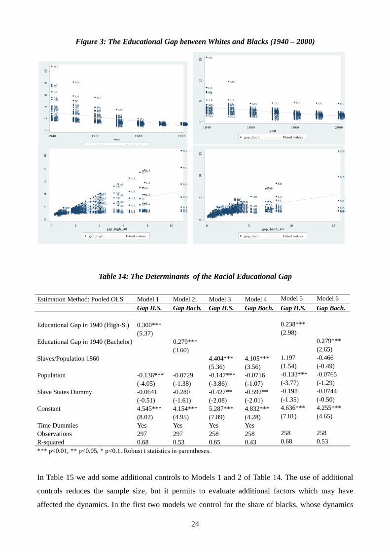
Figure 3 shows the educational gap between whites and blacks calculated as the ratio of the share of

whites to the share of blacks with at least a high-school diploma (on the LHS) or a bachelor degree

(on the RHS). The figure shows a sort of convergence in the share of the population (belonging to

the two groups) with a high-school education. The gap between the shares of whites and blacks

holding a bachelor degree also decreases over time, but this seems to occurs at a slower rate. The

two figures at the bottom show that those states which have started with a larger gap are nowadays

the ones which still have larger racial inequality in terms of education.

In Table 14 we regress the educational gap on the shares of educated whites and blacks in 1940, in a

parsimonious specification where we only control for population and time and regional fixed

effects, in order to use the maximal number of observations. Model 1 shows that the gap in high-

school education depends significantly on the initial gap. At the mean, the educational gap at the

high-school level of education is 0.30 percent higher for a 1 percent increase in the initial gap.

23

Model 2 shows results for the gap between shares of the population holding a bachelor degree.

Decreasing the initial gap for the population holding a bachelor degree by a 1 percent decreases the

gap by almost 0.28 percent. In Models 3 and 4 the fraction of slaves in the population in 1860 has a

significantly positive effect on the racial gaps both at the high-school and bachelor levels. However,

when in Models 4 and 5 we enter this variable together with the initial gaps, it loses significance, as

expected given the pattern of correlation previously mentioned.22 This once again confirms that the

impact of slavery on the evolution of the educational gap runs through its impact on the initial gaps.

To sum up, the results in Table 14 confirm the trend reported in Figure 3, according to which states

which have initiated with a larger racial gap in terms of education still have nowadays a larger racial

educational inequality, if compared to states in which blacks and whites had similar levels of

education.

Table 13: Educational Attainment, by Race (1940-2000):

Descriptive Statistics

All Counties Variable Obs Mean Std. Dev. Min Max High-School Diploma (Whites) 297 60.2291 21.34998 16.37847 94.43 Bachelor Degree (Whites) 297 15.42412 9.624878 2.813198 77.3 High-School Diploma (Blacks) 297 47.18088 26.79546 2.594816 95.9 Bachelor Degree (Blacks) 297 8.758676 6.594131 .3484704 34.82

North of the US Only Variable Obs Mean Std. Dev. Min Max High-School Diploma (Whites) 199 64.82332 20.23654 20.85144 94.43 Bachelor Degree (Whites) 199 16.91558 10.25016 3.544309 77.3 High-School Diploma (Blacks) 199 54.32846 25.12736 5.924223 95.9 Bachelor Degree (Blacks) 199 10.1778 7.026015 1.125535 34.82

South of the US Only Variable Obs Mean Std. Dev. Min Max High-School Diploma (Whites) 98 50.90004 20.58661 16.37847 86.31 Bachelor Degree (Whites) 98 12.39555 7.375334 2.813198 34.73 High-School Diploma (Blacks) 98 32.66692 24.17767 2.594816 78.95 Bachelor Degree (Blacks) 98 5.876993 4.404805 .3484704 20.29

22 In Models 3-6 the number of observations is lower since a few states (e.g., Hawaii, Idaho, Montana) do not appear in the 1860 Census.

24

Figure 3: The Educational Gap between Whites and Blacks (1940 – 2000)

Table 14: The Determinants of the Racial Educational Gap

Estimation Method: Pooled OLS Model 1 Model 2 Model 3 Model 4 Model 5 Model 6 Gap H.S. Gap Bach. Gap H.S. Gap Bach. Gap H.S. Gap Bach. Educational Gap in 1940 (High-S.) 0.300*** 0.238*** (5.37) (2.98) Educational Gap in 1940 (Bachelor) 0.279*** 0.279*** (3.60) (2.65) Slaves/Population 1860 4.404*** 4.105*** 1.197 -0.466 (5.36) (3.56) (1.54) (-0.49) Population -0.136*** -0.0729 -0.147*** -0.0716 -0.133*** -0.0765 (-4.05) (-1.38) (-3.86) (-1.07) (-3.77) (-1.29) Slave States Dummy -0.0641 -0.280 -0.427** -0.592** -0.198 -0.0744 (-0.51) (-1.61) (-2.08) (-2.01) (-1.35) (-0.50) Constant 4.545*** 4.154*** 5.287*** 4.832*** 4.636*** 4.255*** (8.02) (4.95) (7.89) (4.28) (7.81) (4.65) Time Dummies Yes Yes Yes Yes Observations 297 297 258 258 258 258 R-squared 0.68 0.53 0.65 0.43 0.68 0.53 *** p<0.01, ** p<0.05, * p<0.1. Robust t statistics in parentheses. In Table 15 we add some additional controls to Models 1 and 2 of Table 14. The use of additional

controls reduces the sample size, but it permits to evaluate additional factors which may have

affected the dynamics. In the first two models we control for the share of blacks, whose dynamics

AK AK AK AK

AL

AL

ALAL

AL AL AL

AR

AR

AR

AR

AR AR ARAZ

AZ AZ AZCA CA CA CACO CO CO CO

CT CT CT CT CT CT CT

DC

DCDC DC DC DC DC

DEDE

DEDE

DE DE DE

FL

FL

FL

FL

FL FL FL

GA

GA

GA

GA

GA GA GAHI HI HI HI

IA IA IA IA IA IA IAID ID ID ID

IL IL IL IL IL IL IL

IN IN IN IN IN IN INKS KS KS KS KS KS KS

KY KY KY KY KY KY KY

LA

LA

LA

LA

LA LA LAMA MA MA MA MA MA MA

MD

MDMD

MDMD MD MDME ME ME ME

MI MI MI MI MI MI MIMN MN MN MN

MO MO MO MO MO MO MO

MS

MS

MS

MS

MSMS MS

MT MT MT MT

NC

NCNC

NCNC NC NC

ND ND ND ND

NE NE NE NE NE NE NENH NH NH NH

NJNJ

NJ NJ NJ NJ NJNM NM NM NM

NVNV NV NV

NY NY NY NY NY NY NY

OHOH OH OH

OH OH OHOK

OK OK OKOR OR OR OR

P AP A

P A P A P A P A P A

RIRI RI RI RI RI RI

SC

SC

SC

SC

SC SC SCSD SD SD SD

T NT N

T NT N

T N T N T N

T XT X

T XT X

T X T X T XUT

UT UT UT

VAVA

VA

VA VA VA VAVT VT VT VTW A W A W A W A

W IW I

W I W IW I W I W I

W V W V W V W V W V W V W VW Y

W Y W Y W Y

02

46

810

1940 1960 1980 2000year

gap_high Fitted values

AK AKAK AK

AL

AL

AL AL AL AL AL

AR

ARAR AR AR AR AR

AZAZ AZ AZ

CACA CA CACO CO CO CO

CT CT CT CTCT CT CT

DCDC DC

DC DC DC DCDE DE DE

DEDE DE DE

FL

FL

FL FLFL FL FL

GA

GA

GA GAGA GA GAHI HI HI HI

IAIA

IAIA

IA IA IA

ID

ID ID ID

IL IL ILIL

IL IL ILIN IN IN IN IN IN INKSKS

KSKS

KS KS KSKY KY KY KYKY KY KY

LA

LA

LALA LA LA LAMA MA

M AMA

MA MA MA

MDMD

M D MDMD MD MDME ME ME ME

MI MI M I MIMI MI MI

MN MN MN MNMO MO M O MO MO MO MO

MS

MS

M S

MSMS MS MS

MT MT MT MT

NCNC NC NC NC NC NC

ND NDND ND

NE NE NENE

NE NE NENH NH NH NH

NJ NJNJ NJ

NJ NJ NJNM NM NM NM

NV

NV NV NV

NY NY NYNY

NY NY NYOH OH OH OH

OH OH OHOKOK OK OKOR OR OR OR

P AP A

P A P AP A P A P A

RIRI

RIRI

RI RI RI

SC

SC

SC SC SC SC SC

SD SD SD SD

T NT N T N T N T N T N T N

T X T X T X T XT X T X T XUT UT UT UT

VAVA VA VA

VA VA VA

VT VT VT VT

W AW A W A W A

W I

W IW I

W IW I W I W I

W V W V W V W V W V W V W V

W Y

W Y W YW Y

05

1015

1940 1960 1980 2000year

gap_bach Fitted values

AKAKAKAK

AL

AL

ALALALALAL

AR

ARARARARARAR

AZAZAZAZ

CACACACACOCOCOCO

CTCTCTCTCTCTCT

DCDCDC

DCDCDCDCDEDEDEDEDEDEDE

FL

FL

FLFLFLFLFL

GA

GA

GAGAGAGAGAHIHIHIHI

IAIAIAIAIAIAIA

ID

IDIDID

ILILILILILILILINININININININKS

KSKSKSKSKSKSKYKYKYKY

KYKYKY

LA

LA

LALALALALAMAMA

MAMAMAMAMA

MDMDMDMDMDMDMDMEMEMEME

MIMIMIMIMIMIMI

MNMNMNMNMOMOMOMOMOMOMO

MS

MS

MS

MSMSMSMS

MTMTMTMT

NCNCNCNCNCNCNC

NDNDNDND

NENENENENENENE

NHNHNHNH

NJNJNJNJNJNJNJNMNMNMNM

NV

NVNVNV

NYNYNYNYNYNYNYOHOHOHOHOHOHOHOK

OKOKOKOROROROR

P AP AP AP AP AP AP A

RIRI

RIRIRIRIRI

SC

SC

SCSCSCSCSC

SDSDSDSD

T NT NT NT NT NT NT N

T XT XT XT XT XT XT XUTUTUTUT

VAVAVAVAVAVAVA

VTVTVTVT

W AW AW AW A

W I

W IW IW IW IW IW I

W VW VW VW VW VW VW V

W Y

W YW YW Y

05

1015

0 5 10 15gap_bach_40

gap_bach Fitted values

AKAKAKAK

AL

AL

ALALALALAL

AR

AR

AR

AR

ARARARAZAZAZAZCACACACACOCOCOCO

CTCTCTCTCTCTCT

DC

DCDCDCDCDCDC

DEDEDEDEDEDEDE

FL

FL

FL

FL

FLFLFL

GA

GA

GA

GA

GAGAGAHIHIHIHI

IAIAIAIAIAIAIAIDIDIDIDILILILILILILIL

INININININININKSKSKSKSKSKSKS

KYKYKYKYKYKYKY

LA

LA

LA

LA

LALALAMAMAMAMAMAMAMA

MD

MDMDMDMDMDMDMEMEMEME

MIMIMIMIMIMIMIMNMNMNMN

MOMOMOMOMOMOMO

MS

MS

MS

MS

MSMSMS

MTMTMTMT

NC

NCNCNCNCNCNC

NDNDNDND

NENENENENENENENHNHNHNH

NJNJNJNJNJNJNJNMNMNMNM

NVNVNVNV

NYNYNYNYNYNYNY

OHOHOHOHOHOHOH

OKOKOKOKOROROROR

P AP AP AP AP AP AP A

RIRIRIRIRIRIRI

SC

SC

SC

SC

SCSCSCSDSDSDSD

T NT NT NT NT NT NT N

T XT X

T XT XT XT XT X

UTUTUTUT

VAVA

VA

VAVAVAVAVTVTVTVTW AW AW AW A

W IW IW IW IW IW IW I

W VW VW VW VW VW VW VW YW YW YW Y

02

46

810

0 2 4 6 8 10gap_high_40

gap_high Fitted values

25

should capture the massive migration flows occurring across states during this period, and for the

ratio of numbers of farms and manufacturing establishments to the total population, to proxy for

structural changes in the economy.23 The share of blacks marginally explains (being significant at

10 percent) the gap in high-school education, but it is significant in explaining differences between

blacks and whites holding a bachelor degree, denoting that much of the difference in education in

former slave states (the ones with the larger number of blacks) remains at the higher-education

level. The two variables that we use to proxy for structural changes (i.e., the proportion of farms

and manufacturing establishments) are only significant in Model 1. Increasing the proportion of

farms increases the gap in the high-school level of education by 1 percent, while the elasticity

associated with the proportion of manufacturing establishments tends to decrease the gap by almost

2 percent. The latter effect may occur because returns to education in the manufacturing sector are

higher and therefore individuals are more willing to acquire education in the presence of many

manufacturing establishments. Instead in rural areas (with a higher number of farms) returns to

educations are likely to be lower, which associated with land inequality explains the higher

educational gap. The non significance of the same two regressors for the bachelor level, in Model 2,

can be explained by the fact that the latter is less correlated with these two sectors.

Finally in Models 3 and 4 we control for median family income and for the ratio of general direct

expenditure on education to general direct expenditure.24 Richer states tend to have a smaller gap at

the high-school level of education (Model 3), however this is reversed for the bachelor level,

presumably because once gained a high-school diploma whites are more likely to go for further

education when income per capita increases (Model 4). The education share of the general direct

expenditure is only significant in the model for higher education (Model 4). Increasing expenditures

on education by a 1 percent decreases the gap by almost 0.95 percent. The educational gap is

significant in all specifications except Model 4.

To conclude, our results confirm that, over the period under consideration, after controlling for a

large variety of factors, the present level of the racial educational gap is largely explained by the

initial gap, which was in turn determined by slavery through the channels documented in Margo

(1990).

23 The data are collected from the City and County Data-Book and normally refer to three years before the Census (1937, 1947, etc.). 24 These data are also collected from the City and County Data-Book.

26

Table 15: The Determinants of the Racial Educational Gap: Extended Models

Estimation Method: Pooled OLS Model 1 Model 2 Model 3 Model 4 Gap High-Schl. Gap Bach. Dgr. Gap High-Schl. Gap Bach. Dgr. Educational Gap in 1940 (High-School) 0.221*** 0.143*** (2.68) (4.49) Educational Gap in 1940 (Bachelor Degree) 0.180** 0.0356 (2.00) (1.51) Population -0.0947** -0.00761 -0.00604 0.00821 (-2.52) (-0.15) (-0.30) (0.24) Slave States Dummy -0.253 -0.597** -0.173* -0.104 (-1.57) (-2.56) (-1.90) (-1.11) Black Population Share 0.0336* 0.0481*** 0.00705** 0.0376*** (1.85) (4.39) (2.48) (10.27) Number of Farms 0.0104*** 0.00514 (2.84) (0.82) Number of Manufacturing Establish. -0.0209*** 0.000575 (-2.61) (0.04) Median Family Income -0.640** 1.153*** (-2.41) (4.47) Educational Expenditure/Direct General Exp. -0.00178 -0.00946** (-0.53) (-2.19) Constant 3.280*** 2.753*** 7.334*** -7.726*** (5.04) (3.09) (2.98) (-3.48) Time Dummies Yes Yes Yes Yes Observations 238 238 183 183 R-squared 0.76 0.62 0.76 0.68 *** p<0.01, ** p<0.05, * p<0.1. Robust t statistics in parentheses.

7. Conclusion

In this paper we have shown that the institution of slavery still plays a major role in the US

economy and society. The main legacy of slavery is not on the level of development, but on the

degree of inequality. In other words, those US counties that in the past have been more heavily

affected by slave labor turn out to be not poorer, but more unequal, in the present day. We also show

that the current level of income inequality is explained by racial inequality, which is in turn

determined by slavery through its impact on the racial gap in human capital accumulation. While

other factors that have been linked to slavery, such as initial endowments and racial discrimination,

are also shown to affect current inequality, our results suggest that human capital transmission is the

main channel through which slavery manifests its legacy.

In March 2010 President Obama presented Congress with a plan to reform No Child Left Behind

(NCLB), America’s main federal education programme, enacted in 2002 under President Bush with

the full bipartisan support of Congress. Given the apparent failure of the education policies

27

introduced under NCLB, it is likely that the next few months will witness a heated debate about the

state of America’s education system and its weaknesses, among which profound racial and ethnic

educational gaps play a prominent role (Hursh, 2007). Our work shows, on the one hand, that

educational inequality is a central driver of income inequality and, on the other, how deeply rooted

educational inequality is in the history of the country.

REFERENCES

Acemoglu, D., Bautista, M. A., Querubín, P. and Robinson, J. A., 2008, Economic and Political

Inequality in Development: The Case of Cundinamarca, Colombia, in Helpman, E. (ed.),

Institutions and Economic Performance, Harvard University Press, Cambridge, 181–245.

Acemoglu, D., Johnson, S. and Robinson, J. A., 2002, Reversal of Fortune: Geography and

Institutions in the Making of the Modern World Income Distribution, Quarterly Journal of

Economics 117, 1231-1294.

Acemoglu, D., Johnson, S., Robinson, J. A. and Yared, P., 2008, Income and Democracy, American

Economic Review 98, 808-842.

Acemoglu, D. and Robinson, J. A., 2008, Persistence of Power, Elites, and Institutions, American

Economic Review 98, 267-293.

Acemoglu, D. and Wolitzky, A., 2010, The Economics of Labor Coercion, Econometrica,

forthcoming.

Berlin, I., 2003, Generations of Captivity: A History of African American Slaves, Harvard

University Press, Cambridge.

Bobonis, G. J. and Morrow, P. M., 2010, Export Commodity Booms, Labor Coercion, and the

Historical Containment of Education, mimeo, University of Toronto.

Cameron, S. V. and Heckman, J. J., 2001, The Dynamics of Educational Attainment for Blacks,

Hispanics, and Whites, Journal of Political Economy 109, 455-499.

28

Caselli, F. and Coleman, W. J., 2001, The U.S. Structural Transformation and Regional

Convergence: A Reinterpretation, Journal of Political Economy 109, 584-616.

Collins, W. J. and Margo, R. A., 2006, Historical Perspectives on Racial Differences in Schooling

in the United States, in Hanushek, E. and Welch, F. (eds.), Handbook of the Economics of

Education, Elsevier, New York, 107-154.

David, P. A. and Stampp, K. M. (eds.), 1976, Reckoning With Slavery: Critical Essays in the

Quantitative History of American Negro Slavery, Oxford University Press, New York.

Engerman, S. L. and Sokoloff, K. L., 2005a, Institutional and Non-institutionals Explanations of

Economic Differences, in Menard, C. and Shirley, M. M. (eds.), Handbook of New Institutional

Economics, Springer, Dordrecht, 639-665.

Engerman, S. L. and Sokoloff, K. L., 2005b, The Evolution of Suffrage Institutions in the

Americas, Journal of Economic History 65, 891-921.

Engerman, S. L. and. Sokoloff, K. L., 1997, Factor Endowments, Institutions, and Differential Paths

of Growth Among New World Economies: A View from Economic Historians of the United States,

in Harber, S. (ed.), How Latin America Fell Behind, Stanford University Press, Stanford, 260-304.

Fogel, R. W. and Engerman, S. L., 1974, Time on the Cross: The Economics of American Negro

Slavery, Little Brown, Boston.

Galor, O., Moav, O. and Vollrath, D., 2009, Inequality in Landownership, the Emergence of

Human-Capital Promoting Institutions, and the Great Divergence, Review of Economic Studies 76,

143-179.

Goldin, C. and Margo, R. A., 1992, The Great Compression: The US Wage Structure at Mid-

Century, Quarterly Journal of Economics 107, 1-34.

Goldin, C., 1998, America’s Graduation from High School: The Evolution and Spread of Secondary

Schooling in the Twentieth Century, Journal of Economic History 58, 345-374.

29

Goldin, C. and Katz, L. F., 1999, The Shaping of Higher Education: The Formative Years in the

Unites States, 1890 to 1940, Journal of Economic Perspectives 13, 37-62. Heckman, J. J., 1990, The Central Role of the South in Accounting for Economic Progress of Black

Americans, American Economic Review 80, 242-246.

Hursh, D. 2007, Exacerbating Inequality: The Failed Promise of the No Child Left Behind Act,

Race Ethnicity and Education 10, 295-308.

Krueger, A. B. and Lindahl, M., 2001, Education for Growth: Why and For Whom?, Journal of

Economic Literature 39, 1101-1136.

Lagerlöf, N., 2009, Slavery and Other Property Rights, Review of Economic Studies 76, 319-342.

Lagerlöf, N., 2005, Geography, Institutions, and Growth: The United States as a Microcosm,

mimeo, York University.

Lokshin, M. and Sajaia, Z., 2006, EGEN_INEQUAL: Stata Module Providing Extensions to

Generate Inequality and Poverty Measures, Statistical Software Components S456711, Boston

College.

Margo, R. A., 1990, Race and Schooling in the South, 1880-1950: An Economic History, University

of Chicago Press, Chicago.

Mariscal, E. and Sokoloff, K. L., 2000, Schooling, Suffrage, and the Persistence of Inequality in the

Americas, 1800–1945, in Haber, S. (ed.), Political Institutions and Economic Growth in Latin

America: Essays in Policy, History, and Political Economy, Hoover Institution Press, Stanford, 159-

218.

Mitchener, K. J. and McLean, I. W., 2003, The Productivity of U.S. States Since 1880, Journal of

Economic Growth 8, 73-114.

Naidu, S., 2010, Suffrage, Schooling, and Sorting in the Post-Bellum U.S. South, mimeo, Harvard

University.

30

Nunn, N., 2008a, The Long-Term Effects of Africa's Slave Trades, The Quarterly Journal of

Economics 123, 139-176.

Nunn, N., 2008b, Slavery, Inequality, and Economic Development in the Americas: An Examination

of the Engerman-Sokoloff Hypothesis, in Helpman, E. (ed.), Institutions and Economic

Performance, Harvard University Press, Cambridge, 48-180.

Ramcharan, R., 2009, Inequality and Redistribution: Evidence from U.S. Counties and States, 1890-

1930, Review of Economics and Statistics, forthcoming.

Rappaport, J. and Sachs, J. D. , 2003, The United States as a Coastal Nation, Journal of Economic

Growth 8, 5-46.

Sacerdote, B., 2005, Slavery and the Intergenerational Transmission of Human Capital, Review of

Economics and Statistics 87, 217-234.

Smith, J. P., 1984, Race and Human Capital, American Economic Review 74, 685-98.

Smith, J. P. and Welch, F. R., 1989, Black Economic Progress After Myrdal, Journal of Economic

Literature 27, 519-564.

Sokoloff, K. L. and Engerman, S. L., 2000, Institutions, Factor Endowments, and Paths of

Development in the New World, Journal of Economic Perspectives 14, 217-232.

Sokoloff, K. L. and Zolt, E. M., 2007, Inequality and the Evolution of Institutions of Taxation:

Evidence from the Economic History of the Americas, in Edwards, S., Esquivel, G. and Marquez, G.

(eds.), The Decline of Latin American Economies: Growth, Institutions, and Crises, University of

Chicago Press, Chicago, 83-136.

Summerhill, W. , 2010, Colonial Institutions, Slavery, Inequality, and Development: Evidence from

São Paulo, Brazil, MPRA Paper No. 22162.

Vollrath, D., 2010, Inequality and School Funding in the United States, 1890, mimeo, University of

Houston.

31

Table Appendix

Table A1: Returns on Education (Blacks and Whites)

Model 1 Model 2 Dependent Variable: Income (2000) Whites Only Income (2000) Blacks Only Estimation Method: OLS High-School Diploma 0.683*** 0.260*** (4.84) (2.82) Some Years of College (no Bachelor) 0.596*** 0.532*** (2.95) (3.63) Bachelor Degree 1.646*** 0.789*** (11.47) (6.24) Post-Graduate Education (Master or PhD) 1.890*** 1.409*** (8.54) (7.54) Employment Rate 1.601*** 0.368*** (5.62) (2.68) Whites in Labour Force 0.0330*** 0.0778*** (6.31) (6.78) Blacks in Labour Force 0.0134*** 0.0110 (4.42) (1.49) Median Age 0.0109*** 0.0267*** (6.13) (11.03) North East Dummy -0.0165 0.0235 (-0.52) (0.47) South Atlantic Dummy 0.0410 0.0276 (1.55) (0.59) South Central Dummy 0.0388 -0.0720** (1.36) (-2.62) Constant 6.680*** 7.000*** (24.26) (51.20) Sample All Counties All Counties Observations 3030 2714 R-squared 0.77 0.27 *** p<0.01, ** p<0.05, * p<0.1. Robust t statistics in parentheses.

32

Table A2: Robustness Checks for Land Inequality

Dependent Variable: Income Inequality Model 1 Model 2 Estimation Method: OLS IV Slaves/Population 1860 0.0339*** 0.0407*** (6.32) (5.86) Population Density 1860 0.00286*** 0.00154*** (4.57) (5.50) North East Dummy 0.0107*** 0.00708*** (6.12) (3.19) South Atlantic Dummy -0.0198*** -0.0103*** (-8.83) (-3.56) Slave States Dummy 0.0319*** 0.0138*** (16.20) (4.35) Land Inequality 1860 (Gini Index) 0.335*** (7.03) Land Inequality 1860 (GE(0)) 0.0222*** (4.04) Constant 0.377*** 0.241*** (158.59) (11.46) Cragg Donald F-statistic 169.839 Stock and Yogo Critical Values (10% maximal Size) 19.93 Hansen J-Statistic (p-values) 0.0000 Anderson LR-Statistic 163.174 Observations 1878 1878 R-squared 0.31 0.09 *** p<0.01, ** p<0.05, * p<0.1. Robust t statistics in parentheses. Instrument for Model 2: Latitude

Data Appendix

The following datasets have been used:

a) The Historical, Demographic, Economic, and Social Data: The United States, 1790-2000,

downloaded from the Inter-University Consortium for Political and Social Studies

(http://www.icpsr.umich.edu/), is used for the following variables: Total slaves number in 1860,

Total population in 1860, and Size of farms in 1860.

b) The United States Decennial Census 2000, downloaded through the American Fact Finder

(http://factfinder.census.gov/home/saff/main.html?_lang=en), is used for the 2000 levels of:

Households income, Median family income, Shares of population for each race, Total Population,

Median age, Employment rate, and Civilian labor force participation.

33

c) As in Nunn (2008b) data on income per capita are downloaded from the Bureau of Economic

Analysis, Table CA1-3, located at www.bea.gov/regional/reis/.

d) The US Census Bureau, Selected Historical Decennial Census Population and Housing Counts

(www.census.gov/population/www/censusdata/hiscendata.html) is used for data on Education,

Population, and Share of blacks at the state level for the 1940-2000 period.

e) The US City and County Data-Book, which is included in the Historical, Demographic,

Economic, and Social Data, is used for data on Number of farms, Number of manufacturing

establishments, General direct expenditure, and Ratio of education expenditure to general direct

expenditure at the state level for the period 1940-2000.

f) Geographical Dummy Variables are constructed using the US Census regional classification.

g) Inequality measures have been computed as follows, using the STATA package

EGEN_INEQUAL provided by Lokshin and Sajaia (2006):

1) Land Inequality – The Gini index of land inequality is calculated using information about

the size of each farm from the 1860 Census. Sizes of farms fall in the following ranges: (1)

9 acres or less, (2) 10 to 19 acres, (3) 20 to 49 acres, (4) 50 to 99 acres, (5) 100 to 499 acres,

(6) 500 to 999 acres, and (7) 1,000 acres or more. Since for each category we do not know

the mean farm size, we assume that farms are uniformly distributed within each category

and then we take the mean size for the category. As in Nunn (2008b) and Lagerlöf (2005),

for the category 1,000 acres or more we use 1,000 acres.

2) Income Inequality – The Gini index of income inequality is calculated using data from the

2000 CENSUS (downloaded through the US Fact Finder). We adopt the CENSUS

categories and we assume that households within each category are uniformly distributed, so

that in order to find the Gini index we take the mean value. For the category $200,000 or

more we take $200,000.

3) Racial Income Inequality - This is the Gini index for income per capita in 2000 (CENSUS

2000) for each race in the Census. Using information on classes of income for each race we

obtain a horizontal Gini index to calculate the distribution of income across races.

34

4 ) Racial Educational Inequality – Data on educational attainment are downloaded from the

National Center for Education Statistics. For each race we have data on the share of the

population with: 1) no high-school diploma (0-9 grade but no diploma); 2) with a high-

school diploma; 3) with some years of college (but no degree); 4) with an undergraduate

degree; 5) with a master’s degree; 5) with a PhD. We code this information as follows: 1, if

the individual did not gain a high-school diploma; 2, if he has a high-school diploma; 3, if

he has some years of colleges; 4, if he has an undergraduate degree; and so on. We use this

coding rule to calculate the Gini index across races.