Slave Trade and Development by Temitope G. Ogunsanmi · Slave Trade and Development by Temitope G....

1

Slave Trade and Development

by Temitope G. Ogunsanmi

(8125922)

Major paper presented to the

Department of Economics of the University of Ottawa

in partial fulfillment of the requirements of M.A. Degree

Supervisor: Professor Jason Garred

ECO 6999

Ottawa, Ontario

December 2016

2

ABSTRACT

Using data for 38 countries, I estimate the impact of slave trades on individual components of

GDP. I observe three important pieces of evidence that countries greatly affected by slave

exports are less developed today. Firstly, I find that countries with more slave exports spend a

smaller share of GDP on government purchases. This finding is consistent with Wagner’s law in

that more developed countries tend to allocate a larger share of GDP on government

expenditure. I also find weak evidence that these countries spend less on health and education

which implies low investment in human capital in these countries. Secondly, I find that countries

that exported more slaves are more dependent on agriculture. These countries have not

experienced structural transformation to the same extent as developed countries. Finally, I find

no evidence that countries that exported more slaves are more dependent on aid.

3

SECTION ONE

INTRODUCTION

Various research has been conducted over time on the effect of historical events on certain

factors today of which current economic development is of utmost interest. Africa’s historical

events, especially the slave trades and colonialism, have captured the interest of many

researchers. Between 1400 and 1900, Africa as a continent experienced four different slave

trades: the Trans-Atlantic, Trans-Saharan, Indian Ocean and Red Sea slave trades. During this

period, slaves were exported from different parts of Africa to the locations of slave demand.

Using Nunn’s paper “The Long-Term Effects of Africa’s Slave Trades” (2008) as my major

reference, I provide an empirical examination of the impact of Africa’s slave trades on individual

components of GDP. Nunn used shipping records and GDP data (Maddison, 2003) for 52

countries to estimate the impact of slave trades on economic development today. He also used an

analysis of selection into slave trades and variation in sailing distances to the location of demand

(instrumental variables) to better understand if this relationship is causal or spurious. He found

that countries that had higher population density (which is an indicator of economic prosperity)

in 1400 selected into the slave trades. Both the OLS and instrumental variables (IV) estimates

suggested that the more slaves that were exported by a country the worse its economic

performance today.

I extend the argument that countries that were greatly affected by slave exports are less

developed today. I use data on some of the individual components of GDP from the World Bank

as my dependent variables and use slave exports per land area and controls used by Nunn for

independent variables, as well as reproducing his IV strategy. The dependent variables include

4

consumption, investment, government expenditure, health, education, agriculture, industry,

services, manufacturing, total natural resources rents and net official development assistance

(ODA), all of which are explained in detail in section III of this paper. My goal is to see how

these individual components of GDP (beyond GDP alone) are affected by slave trades.

I link my findings to Wagner’s law and structural transformation based on my findings. The

development of an economy will be accompanied by an increased share of public expenditure in

gross national product (GNP) states Wagner’s law, and a shift from agriculture to other sectors of

the economy (industry and services) according to the theories of structural transformation

(Kuznets, 1957). Since my argument is that countries affected by more slave exports are less

developed today, Wagner’s law predicts that these countries spend a smaller share of GDP on

government purchases (less government spending) and structural transformation predicts more

dependence on agriculture in these countries. I also expect that more slave export countries are

more dependent on aid.

Firstly, I observe very similar results to those of Nunn (a negative and significant effect of slave

trades on current GDP per capita) despite the differences in the datasets used and in the number

of countries used in my research. I also discover that countries that exported more slaves, which

are less developed today, have a lower share of government spending. This is in line with the

Wagner’s law prediction that less developed countries spend a smaller share of GDP on

government purchases. Estimating the impact of slave trades on public spending on health and

education, I find weak evidence that countries affected by high slave exports spend less on health

and education as a share of GDP. This connotes that these countries investment on human capital

is low.

5

Another interesting finding is that countries that exported more slaves are more dependent on

agriculture. I observe that the coefficient estimates for agriculture share of GDP is positive while

for industry and services they are negative. Based on the expectation that countries with more

slave exports are more agriculture dependent, this also means that these countries are less

dependent on industry and services (the countries have not experienced structural change). It

should however be noted that the coefficients for industry are not significant while services

coefficients are only significant in two specifications.

Lastly, in contrast to what I expected, I find no relationship between slave trades and aid.

Although countries that exported more slaves during the slave trades are less developed today, it

does not seem to be true that these countries are more dependent on aid (official development

assistance).

This paper is a contribution to the literature as it looks not only at the impact of slave exports on

current development but also the impact of slave exports on key characteristics of economic

development. There are similar studies on slave trades apart from the Nunn (2008) paper. Fenske

and Kala (2015) estimated the impact of climate on slave exports. They found substantial

evidence that the colder the weather, the more slaves were exported during the slave trades.

Nunn and Wantchekon (2011) on the other hand found that less trusting people today are those

whose ancestors were more affected by the slave trades.

The paper is structured as follows. Section II provides a summary of relevant empirical literature

including past and present research. Section III gives detailed information about the data sources

and definitions. Section IV describes the empirical specifications and Section V discusses the

results. Section VI gives the conclusion.

6

SECTION TWO

LITERATURE REVIEW

The aim of this section is to discuss Nunn’s paper and other slave trade papers, history and

development papers, papers on Wagner’s law and structural transformation papers in detail.

Nunn’s paper is discussed because it is a major reference for my research and will be followed

by other studies on slave trades. I will also continue to discuss the importance of history on

today’s development by looking at three major papers cited by Nunn 2009 (Acemoglu et al.

(2001), La Porta et al (1997; 1998), and Engerman and Sokoloff (1997; 2002) and other research

related to these. Finally, I will discuss government expenditure using Wagner’s law and

structural transformation in relation to agriculture in different subsections and other findings

related to each of these.

Nunn (2008) and other slave papers

Africa as a continent experienced four major slave trades between 1400 and 1900 of which the

largest was the trans-Atlantic slave trades. The other three slave trades in no specific order that

were prior to the trans-Atlantic slave trades are the trans-Saharan, Red Sea and Indian Ocean

slave trades. What made Africa’s slave trades unique relative to other slave trades is the large

number of slaves traded during that period and the fact that individuals of the same ethnicities

enslaved one another (Nunn 2008).

Nunn (2008) in the introduction of his paper sought to answer the question of whether Africa’s

current performance can be explained by two main historical events: slave trades and

colonialism. Focusing on slave trades, he used data from shipping records and historical

documents reporting slave ethnicities to construct estimates of the number of slaves exported

7

from each country and real per capita GDP from Maddison (2003). He found a robust negative

relationship between the number of slaves exported and subsequent economic performance.

To know if there is a causal effect on slave trades on income, he used two different approaches.

The first approach was to use historical data and evidence from African historians to evaluate the

importance and characteristics of selection into slave trades. He found that societies or countries

that had higher population density in 1400, which is as an indicator of economic development,

were the ones that selected into slave trades. The second approach he used was using sailing

distance from each country to locations of demand for slaves as instruments for slave exports per

area. The instrumental variables (IV) results confirm the OLS estimates, suggesting that more

extraction of slaves during the slave trades resulted in worse economic performance.

Examining the channels of causality between slave exports and economic development, he

documented that consistent with historical accounts, slave trades hindered the creation of broader

ethnic groups which led to ethnic fractionalization and also resulted in the creation of weak and

underdeveloped political structures. This is consistent with the findings of Alesina et al. (2003)

that ethnic fractionalization variables are likely to be an important determinant of economic

success and institutional quality. Similarly, Easterly and Levine (1997) found that ethnic

diversity is very important in determining economic development as it is associated with low

schooling, insufficient infrastructure and underdeveloped financial systems.

Slave exports created a culture of mistrust in Africa (Nunn and Wantchekon 2011). Combining

individual-level survey data with historical data on slave shipments by ethnic group, Nunn and

Wantchekon (2011) find that individuals whose ancestors were more affected by slave exports

are less trusting today as slave trading adversely affected individuals’ trust of those around them.

They found a robust positive relationship between distance from the coast in Africa and trust. In

8

the words of Nunn and Wantchekon (2011), “the effects of slave trade penetrated deep into the

social fabric of societies and eventually turned friends, families, neighbours against each other.”

Did climate determine the number of slaves exported during the slave trade era? Fenske and Kala

(2015) answered this question by examining the relationship between climate and slave trades.

They used a combination of data on temperature, trans-Atlantic slave trade and agro-ecological

zones which classify land into zones based on climate, elevation, soils and latitude. Using the

histories of Whydah, Benguela, and Mozambique to support their interpretation, they found a

large effect of climate change on slave exports; a one degree increase in temperature reduced

annual exports by roughly 3000 slaves per port. An explanation for this given by the authors is

that lower temperatures reduced mortality and raised agricultural yields thereby lowering slave

supply costs and increasing number of slaves exported. They conclude that cold weather shocks

at the peak of the slave trade (which caused slave exports to increase) predict lower economic

activity today.

History and Development

Are historical events important to today’s economic performance? Can these events explain why

economic development in Africa has not improved over time? What are the actual effects of

these events on current development? These questions and many more have been of utmost

interest to historical and development authors and have been answered in various ways. The

major African historical events were slave trades and colonialism.

Acemoglu et al. (2001) examined the effect of institutions on current economic performance

using mortality rates faced by settlers as an instrument for current institutions. Not all colonies

were conducive for colonists to settle as some colonies had disease environments causing death

9

of Europeans. In colonies where colonist could settle, replicas of European institutions were

created with a great emphasis on private property and checks against power while in colonies

with worse disease environments, extractive (bad) states were created. Extractive states do not

provide much protection for private property nor checks and balances against government

appropriation. Instead, the main purpose of creating the extractive state was to transfer as many

resources as possible from the colony to the colonizer with minimum investment. They found

that institutions where Europeans could settle do better in current economic performance than

those in which the extractive states were created. Their estimates implied that differences in

institutions account for roughly three-quarters of differences in income per capita.

Consistent with the findings of Acemoglu et al. (2001) on the impact of institutions on current

economic performance, Banerjee and Iyer (2005) examined the impact of the colonial land

revenue system set up by the British in India. Land revenues were a major source of income for

all governments of India including the British at that time. In some areas, “landlords” were in

charge of collecting revenues from individual cultivators and thereafter, the revenues were

remitted to the British. In some other areas, revenue arrangements were made directly with the

individual cultivator. They found that areas in which property rights were originally given to the

landlords have significant lower investments and productivity in agriculture than areas whose

property rights were historically given to individual cultivators.

Observing 49 countries that have publicly traded companies, La Porta et al. (1997; 1998)

examined the effect of the strength of legal rules protecting investor rights on financial

development using historical differences between the British common law, Roman civil law,

German civil law and Scandinavian civil law. They hypothesized that differences in the type and

success of financial systems around the world could be traced in part to the differences in

10

investor protections against expropriation by insiders. Their result showed that countries with

common law system have greater investor (shareholders and creditors) protection relative to

countries with civil law, French civil law being at the bottom of the scale (that is, providing the

weakest legal protections of investors). They also stated that public and private institutions are

less effective in countries displaying low levels of trust among citizens.

The argument of Engerman and Sokoloff (1997; 2002) was that different development

experiences of the countries in the Americas can be explained by initial differences in land

endowments and geography suitable for growing crops that can be traded globally. These crops

like sugar are best grown on large-scale plantations using slave labour, leading to inequality.

Former Spanish colonies in Mexico and Peru had rich endowments of mineral resources,

however this further strengthened the tendency towards political and economic inequality.

Severe economic and political inequality resulted in the eventual evolution of domestic

institutions that preserved the rights of the gentry and constrained the participation of the

remaining population.

Government spending and Wagner’s Law

The development of an industrial economy will be accompanied by an increased share of public

expenditure in gross national product (GNP) states Wagner’s law. In other words, the more an

economy develops the higher the share of government spending in that economy.

Using Government Financial Statistics data from IMF that covered over 100 countries from

1970-2000, Shelton (2007) looked at cross-sectional and intertemporal variation in government

expenditures and both individual categories of expenditure and different levels of government.

One of the interesting results found was that Wagner’s law was shown to be driven by

11

demographics in that richer countries are older and spend more on social security than poorer

countries.

However, Durevall and Henrekson’s (2011) findings were not consistent with Wagner’s

hypothesis. They carried out a critical appraisal of two contending theories intending to explain

long-run government spending: Wagner’s law and various versions of the ratchet effect (the idea

that government expenditure declines more slowly during a crisis than per capita income so that

government spending per unit output rises). Analysing data for two countries, Sweden and the

UK, they found that Wagner’s law was not a stylized fact for how economies behaved in the

long-run although the law seemed to hold reasonably well over a period when the economy goes

through a process of modernization.

Mohammadi et al. (2008) using annual data for Turkey over 1950 to 2005 provide strong support

for the validity of Wagner’s law. They further explain that the law applies primarily to the period

of emerging societies and that the underlying premise of the law is based on the role of

government as a provider of public goods. From their results, the predictions were clearly

reflected in the role of government in Turkey as the Turkish government embarked on a new

development strategy designed to improve the infrastructure of the country through an increase

in the level of public investment in 1983.

Structural Transformation

Agriculture as a sectoral component of GDP tends to be more important in developing countries

as compared to other sectors (industry and services). This could be explained as a result of

structural transformation (when a country changes from subsistence agriculture to urban

manufacturing and services). Kuznets (1957) explains structural transformation as a shift from

12

agriculture to other sectors (as a form of urbanization) and a numerous corollaries which the

change in mode of life implies; it could also mean a shift from small, individually managed

enterprises, to large-scale productive units, often organized in even larger economic management

units.

Uniting Kuznets structural transformation idea to the Kaldor stylized facts in that a massive

reallocation of labor from agriculture into manufacturing and services will accompany the

growth process of a country, Kongsamut, Rebelo and Xie (2001) find that the generalized

balanced growth model proposed by them is not consistent with the regularity of this growth

process. Although they find evidence of sectoral reallocation of employment out of agriculture

into services for all growing countries, they mention that this reallocation of labor out of

agriculture has been limited since the 1970’s and that the expansion of service employment has

slowed down.

In contrast to the results obtained by Kongsamut, Rebelo and Xie (2001), Ngai and Pissarides

(2007) found results that are consistent with the long-run evidence of Kuznets. Given the

assumption that final goods produced by each sector are not easily substitutable, the differences

in total factor productivity (TFP) growth rates across sectors predict sectoral employment

changes. Their model predicted that labour would move from the sector with low TFP growth to

sectors with high TFP growth.

Duarte and Restuccia (2010) measure sectoral labour productivity across countries using a model

of structural transformation. They found productivity differences across countries to be large in

agriculture and services and smaller in manufacturing and that production gaps have

substantially reduced over time in agriculture and industry but not so much in services. They also

found that productivity catch-up in industry explained about 50% of gains in aggregate

13

productivity across countries but the catch-up in services is low. They stated that the lack of

catch-up in services explain all the experiences of slowdown, stagnation and decline observed

across countries.

14

SECTION THREE

DATA

I use data from the World Bank’s “World Development Indicators” and Nathan Nunn’s “The

Long-term Effects of Africa’s Slave Trades (2008)” for the purpose of this major research paper.

Data used to construct the dependent variables, which is sourced from the World Development

Indicators (WDI) for the year 2000, are grouped into three categories. Before stating the

variables used in each category, I first note that I use total GDP per capita adjusted for

purchasing power parity (PPP). I use GDP per capita itself in order to compare this paper’s result

to Nunn’s. The first category of dependent variables not studied by Nunn is the expenditure

components of Gross Domestic Product (GDP) which consist of household consumption

expenditure, government expenditure, and gross fixed capital formation (investment).

The second category is the sectoral components of GDP, consisting of agriculture, industry and

services, along with separate variables for manufacturing and total natural resource rents. I also

include variables for government spending on health and education as a share of GDP. Total

natural resources rents as defined by WDI is the sum of oil rents, natural gas rents, coal rents

(hard and soft), mineral rents and forest rents, calculated as the difference between the price of a

commodity and the average cost of producing it.

The last category which consists of only one variable is the net official development assistance

(ODA) received as a percentage of Gross National Income (GNI). The net ODA received as

described by WDI consists of disbursements of loans made on concessional terms and grants by

official agencies of members of Development Assistance Committee (DAC), by multilateral

15

institutions and by non-DAC countries to promote economic development and welfare in

countries and territories in the DAC list of ODA recipients.

I used the same data for independent variables and the same set of controls used by Nathan Nunn

in The Long-term Effects of Africa’s Slave Trades (2008). The independent variable is the

natural log of the total number of slaves exported between 1400 and 1900 normalized by land

area.

The controls include colonizer country fixed effects and other variables that capture country

differences such as distance from the equator, longitude, minimum monthly rainfall, average

maximum humidity, average minimum temperature, proximity to the ocean measured by the

natural log of coastline divided by land area, island and North African country dummies,

percentage of Islamic population in a country, French legal origin and country endowment

differences (which includes the natural log of the annual average per capita production between

1970 and 2000 of gold, oil and diamonds). Other variables taken from Nathan Nunn’s paper

include distances from each African country to where slaves were demanded (via the Atlantic,

Indian Ocean, Red Sea, and Trans-Saharan slave trades) which are used as instruments.

Although 52 countries were represented in Nathan Nunn’s paper, I consider a smaller sample due

to insufficient data for the dependent variables. Specifically, data is available for the expenditure,

sectoral components of GDP, health spending and net ODA for only 38 countries, and data on

education spending is available for only 24 countries.

16

SECTION FOUR

EMPIRICAL SPECIFICATIONS

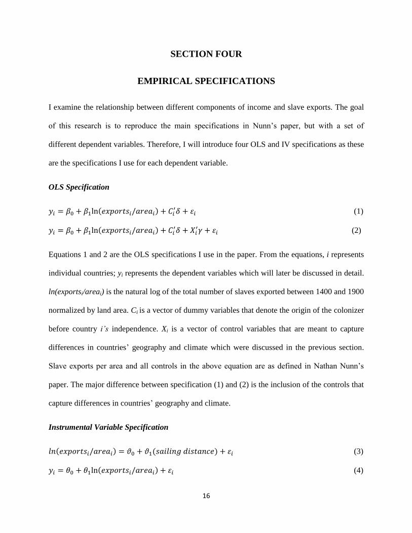
I examine the relationship between different components of income and slave exports. The goal

of this research is to reproduce the main specifications in Nunn’s paper, but with a set of

different dependent variables. Therefore, I will introduce four OLS and IV specifications as these

are the specifications I use for each dependent variable.

OLS Specification

𝑦𝑖 = 𝛽0 + 𝛽1ln(𝑒𝑥𝑝𝑜𝑟𝑡𝑠𝑖/𝑎𝑟𝑒𝑎𝑖) + 𝐶𝑖′𝛿 + 휀𝑖 (1)

𝑦𝑖 = 𝛽0 + 𝛽1ln(𝑒𝑥𝑝𝑜𝑟𝑡𝑠𝑖/𝑎𝑟𝑒𝑎𝑖) + 𝐶𝑖′𝛿 + 𝑋𝑖

′𝛾 + 휀𝑖 (2)

Equations 1 and 2 are the OLS specifications I use in the paper. From the equations, i represents

individual countries; yi represents the dependent variables which will later be discussed in detail.

ln(exportsi/areai) is the natural log of the total number of slaves exported between 1400 and 1900

normalized by land area. Ci is a vector of dummy variables that denote the origin of the colonizer

before country i’s independence. Xi is a vector of control variables that are meant to capture

differences in countries’ geography and climate which were discussed in the previous section.

Slave exports per area and all controls in the above equation are as defined in Nathan Nunn’s

paper. The major difference between specification (1) and (2) is the inclusion of the controls that

capture differences in countries’ geography and climate.

Instrumental Variable Specification

𝑙𝑛(𝑒𝑥𝑝𝑜𝑟𝑡𝑠𝑖/𝑎𝑟𝑒𝑎𝑖) = 𝜗0 + 𝜗1(𝑠𝑎𝑖𝑙𝑖𝑛𝑔𝑑𝑖𝑠𝑡𝑎𝑛𝑐𝑒) + 휀𝑖 (3)

𝑦𝑖 = 𝜃0 + 𝜃1ln(𝑒𝑥𝑝𝑜𝑟𝑡𝑠𝑖/𝑎𝑟𝑒𝑎𝑖) + 휀𝑖 (4)

17

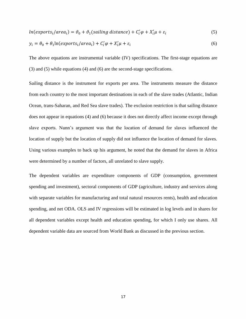
𝑙𝑛(𝑒𝑥𝑝𝑜𝑟𝑡𝑠𝑖/𝑎𝑟𝑒𝑎𝑖) = 𝜗0 + 𝜗1(𝑠𝑎𝑖𝑙𝑖𝑛𝑔𝑑𝑖𝑠𝑡𝑎𝑛𝑐𝑒) + 𝐶𝑖′𝜑 + 𝑋𝑖

′𝜇 + 휀𝑖 (5)

𝑦𝑖 = 𝜃0 + 𝜃1ln(𝑒𝑥𝑝𝑜𝑟𝑡𝑠𝑖/𝑎𝑟𝑒𝑎𝑖) + 𝐶𝑖′𝜑 + 𝑋𝑖

′𝜇 + 휀𝑖 (6)

The above equations are instrumental variable (IV) specifications. The first-stage equations are

(3) and (5) while equations (4) and (6) are the second-stage specifications.

Sailing distance is the instrument for exports per area. The instruments measure the distance

from each country to the most important destinations in each of the slave trades (Atlantic, Indian

Ocean, trans-Saharan, and Red Sea slave trades). The exclusion restriction is that sailing distance

does not appear in equations (4) and (6) because it does not directly affect income except through

slave exports. Nunn’s argument was that the location of demand for slaves influenced the

location of supply but the location of supply did not influence the location of demand for slaves.

Using various examples to back up his argument, he noted that the demand for slaves in Africa

were determined by a number of factors, all unrelated to slave supply.

The dependent variables are expenditure components of GDP (consumption, government

spending and investment), sectoral components of GDP (agriculture, industry and services along

with separate variables for manufacturing and total natural resources rents), health and education

spending, and net ODA. OLS and IV regressions will be estimated in log levels and in shares for

all dependent variables except health and education spending, for which I only use shares. All

dependent variable data are sourced from World Bank as discussed in the previous section.

18

SECTION FIVE

RESULTS

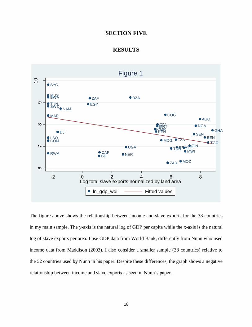
The figure above shows the relationship between income and slave exports for the 38 countries

in my main sample. The y-axis is the natural log of GDP per capita while the x-axis is the natural

log of slave exports per area. I use GDP data from World Bank, differently from Nunn who used

income data from Maddison (2003). I also consider a smaller sample (38 countries) relative to

the 52 countries used by Nunn in his paper. Despite these differences, the graph shows a negative

relationship between income and slave exports as seen in Nunn’s paper.

AGO

BDI

BEN

BFA

BWA

CAF

CIV

CMR

COG

COM

DJI

DZA

EGY

GHA

GIN

KEN

LSO

MAR

MDG

MOZ

MRT

MUS

MWI

NAM

NER

NGA

RWA

SEN

SLE

SWZ

SYC

TCD

TGO

TUN

TZA

UGA

ZAF

ZAR

67

89

10

-2 0 2 4 6 8Log total slave exports normalized by land area

ln_gdp_wdi Fitted values

Figure 1

19

TABLE I

COMPARISON BETWEEN NUNN'S RESULT AND THIS PAPER'S

DEPENDENT VARIABLE: GDP

NUNN THIS PAPER

PANEL A: OLS with colony controls

ln (export/area) -0.112 -0.116

[0.024] [0.033]

PANEL B: OLS with full controls


[0.034] [0.043]

PANEL C: IV


[0.053] [0.053]

PANEL D: IV with full controls


[0.153] [0.194]

Notes. OLS and IV estimates reported. The dependent variable is the natural log of GDP per capita in 2000. Nunn's paper

used 52 countries which data was sourced from Maddison (2003) but this paper uses 38 countries, data sourced from WDI.

The figures in brackets are robust standard errors.

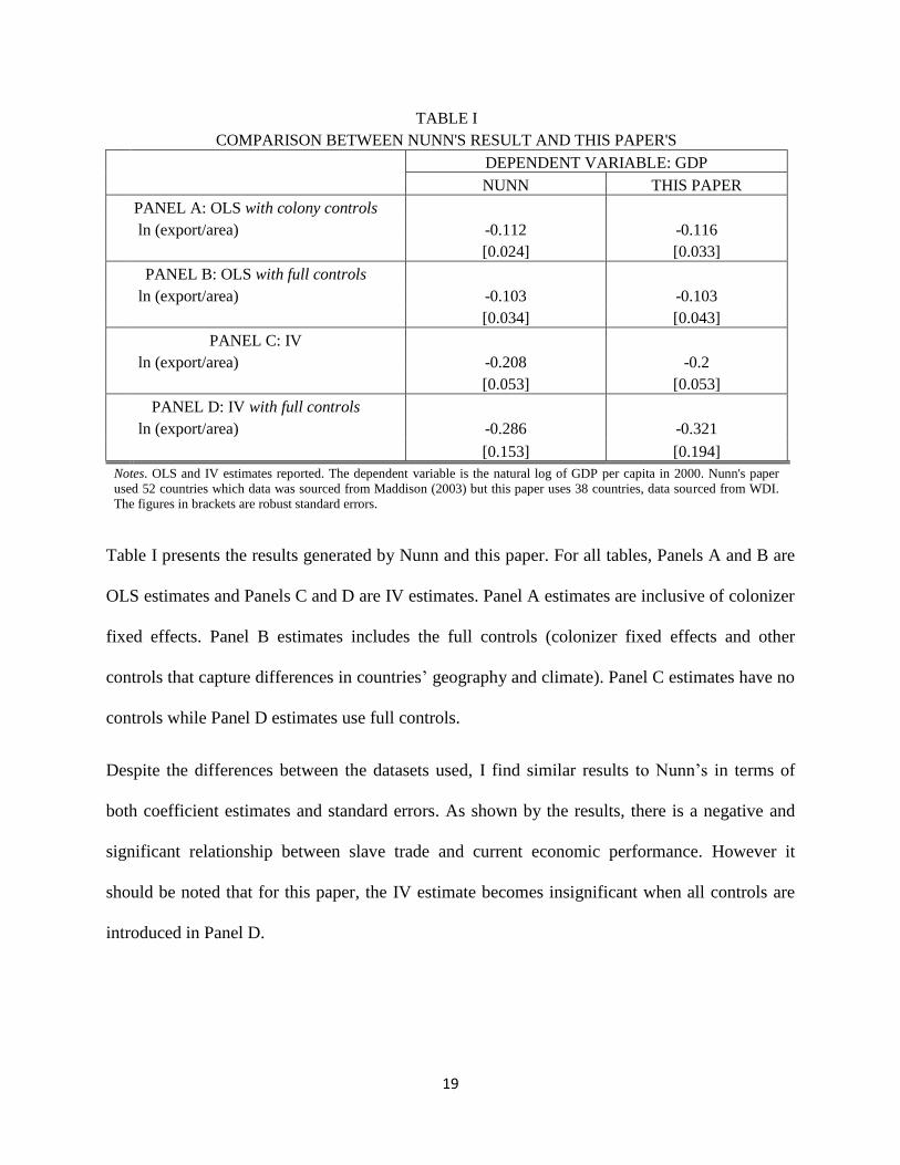
Table I presents the results generated by Nunn and this paper. For all tables, Panels A and B are

OLS estimates and Panels C and D are IV estimates. Panel A estimates are inclusive of colonizer

fixed effects. Panel B estimates includes the full controls (colonizer fixed effects and other

controls that capture differences in countries’ geography and climate). Panel C estimates have no

controls while Panel D estimates use full controls.

Despite the differences between the datasets used, I find similar results to Nunn’s in terms of

both coefficient estimates and standard errors. As shown by the results, there is a negative and

significant relationship between slave trade and current economic performance. However it

should be noted that for this paper, the IV estimate becomes insignificant when all controls are

introduced in Panel D.

20

TABLE II

RELATIONSHIP BETWEEN SLAVE EXPORTS AND COMPONENT LEVELS OF GDP

DEPENDENT VARIABLES

CONSUMPTION GOVERNMENT INVESTMENT

PANEL A: OLS with

colony controls

ln (export/area) -0.102 -0.19 -0.153

[0.023] [0.038] [0.051]

PANEL B: OLS with

full controls

ln (export/area) -0.084 -0.247 -0.099

[0.034] [0.061] [0.071]

PANEL C: IV

ln (export/area) -0.17 -0.283 -0.251

[0.043] [0.058] [0.073]

PANEL D: IV with full

controls

ln (export/area) -0.202 -0.512 -0.364

[0.116] [0.244] [0.234]

Notes. OLS and IV estimates are reported for the component levels of GDP. The dependent variables are natural log of

consumption expenditure, government expenditure and investment for the year 2000 for 38 countries. The figures in brackets

are robust standard errors.

Table II shows the relationship between slave exports and expenditure component levels of GDP

which is the natural log of consumption expenditure, government expenditure and investment.

The result above is in line with the basic Nunn results in that the OLS and IV estimates show a

negative relationship between each of the expenditure components of GDP and slave exports.

The OLS and IV estimates for all variables are statistically significant with the exception of

investment which becomes insignificant when all controls are added in the OLS and IV estimates

(Panel B and Panel D).

21

TABLE III

RELATIONSHIP BETWEEN SLAVE EXPORTS AND COMPONENT SHARES OF GDP

DEPENDENT VARIABLES

CONSUMPTION GOVERNMENT INVESTMENT

PANEL A: OLS with

colony controls

ln (export/area) 0.784 -1.145 -0.529

[0.910] [0.346] [0.374]

PANEL B: OLS with full

controls

ln (export/area) 0.496 -2.022 -0.46

[0.984] [0.462] [0.472]

PANEL C: IV

Slave export/area 1.674 -1.434 -0.636

[1.089] [0.464] [0.452]

PANEL D: IV with full

controls

ln (export/area) 6.058 -3.142 0.588

[4.688] [1.434] [1.057]

Notes. OLS and IV estimates are reported for the component shares of GDP. The dependent variables are component

(consumption expenditure, government expenditure and investment) share of GDP for the year 2000 for 38 countries. The

figures in brackets are robust standard errors.

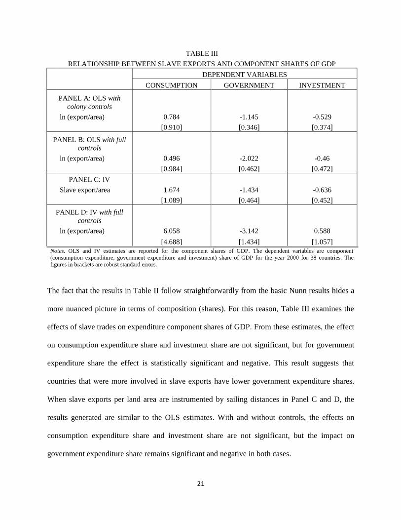
The fact that the results in Table II follow straightforwardly from the basic Nunn results hides a

more nuanced picture in terms of composition (shares). For this reason, Table III examines the

effects of slave trades on expenditure component shares of GDP. From these estimates, the effect

on consumption expenditure share and investment share are not significant, but for government

expenditure share the effect is statistically significant and negative. This result suggests that

countries that were more involved in slave exports have lower government expenditure shares.

When slave exports per land area are instrumented by sailing distances in Panel C and D, the

results generated are similar to the OLS estimates. With and without controls, the effects on

consumption expenditure share and investment share are not significant, but the impact on

government expenditure share remains significant and negative in both cases.

22

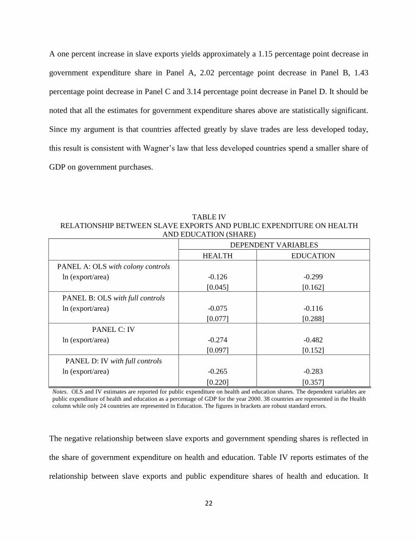
A one percent increase in slave exports yields approximately a 1.15 percentage point decrease in

government expenditure share in Panel A, 2.02 percentage point decrease in Panel B, 1.43

percentage point decrease in Panel C and 3.14 percentage point decrease in Panel D. It should be

noted that all the estimates for government expenditure shares above are statistically significant.

Since my argument is that countries affected greatly by slave trades are less developed today,

this result is consistent with Wagner’s law that less developed countries spend a smaller share of

GDP on government purchases.

TABLE IV

RELATIONSHIP BETWEEN SLAVE EXPORTS AND PUBLIC EXPENDITURE ON HEALTH

AND EDUCATION (SHARE)

DEPENDENT VARIABLES

HEALTH EDUCATION



[0.045] [0.162]



[0.077] [0.288]

PANEL C: IV


[0.097] [0.152]



[0.220] [0.357]

Notes. OLS and IV estimates are reported for public expenditure on health and education shares. The dependent variables are

public expenditure of health and education as a percentage of GDP for the year 2000. 38 countries are represented in the Health

column while only 24 countries are represented in Education. The figures in brackets are robust standard errors.

The negative relationship between slave exports and government spending shares is reflected in

the share of government expenditure on health and education. Table IV reports estimates of the

relationship between slave exports and public expenditure shares of health and education. It

23

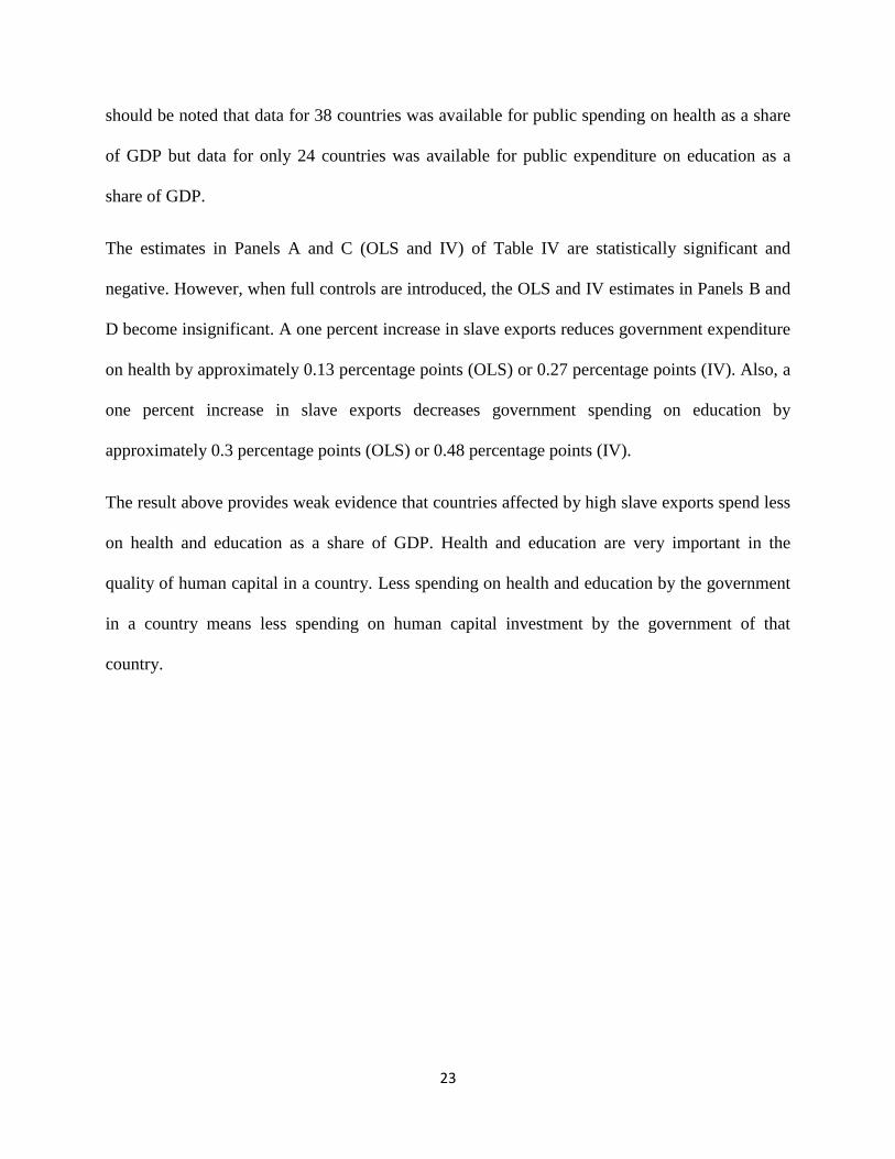
should be noted that data for 38 countries was available for public spending on health as a share

of GDP but data for only 24 countries was available for public expenditure on education as a

share of GDP.

The estimates in Panels A and C (OLS and IV) of Table IV are statistically significant and

negative. However, when full controls are introduced, the OLS and IV estimates in Panels B and

D become insignificant. A one percent increase in slave exports reduces government expenditure

on health by approximately 0.13 percentage points (OLS) or 0.27 percentage points (IV). Also, a

one percent increase in slave exports decreases government spending on education by

approximately 0.3 percentage points (OLS) or 0.48 percentage points (IV).

The result above provides weak evidence that countries affected by high slave exports spend less

on health and education as a share of GDP. Health and education are very important in the

quality of human capital in a country. Less spending on health and education by the government

in a country means less spending on human capital investment by the government of that

country.

24

TABLE V

RELATIONSHIP BETWEEN SLAVE EXPORTS AND SECTORAL COMPONENT LEVEL OF GDP

DEPENDENT VARIABLES

AGRICULTURE INDUSTRY SERVICES MANUFACTURING RENTS

PANEL A: OLS

with colony

controls

ln (export/area) 0.005 -0.117 -0.16 -0.148 0.119

[0.027] [0.046] [0.036] [0.056] [0.061]

PANEL B: OLS

with full controls

ln (export/area) 0.046 -0.143 -0.112 -0.082 0.033

[0.038] [0.055] [0.057] [0.075] [0.079]

PANEL C: IV

ln (export/area) -0.006 -0.23 -0.256 -0.253 0.067

[0.046] [0.075] [0.054] [0.082] [0.094]

PANEL D: IV

with full controls

ln (export/area) -0.055 -0.488 -0.295 -0.255 -0.424

[0.117] [0.303] [0.162] [0.190] [0.398]

Notes. OLS and IV estimates are reported for the sectoral components levels of GDP. The dependent variables are natural log

of agriculture, manufacturing, industry, services and total natural resource rents for the year 2000 for 38 countries. The figures

in brackets are robust standard errors.

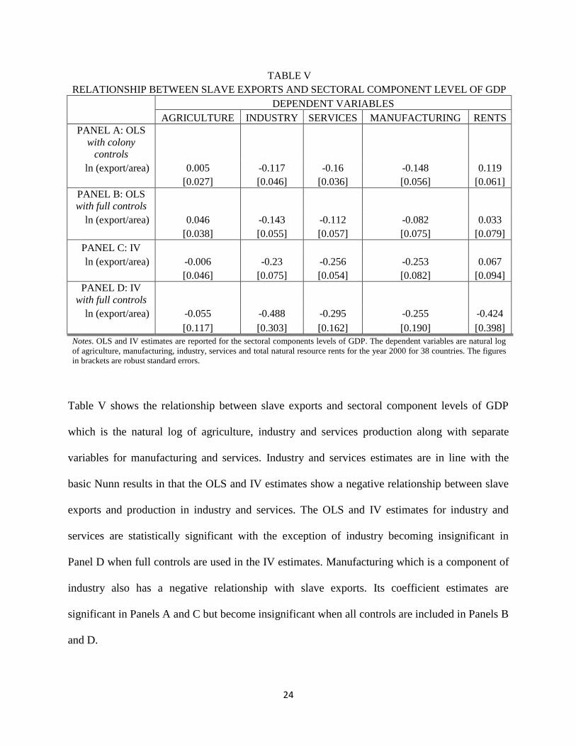
Table V shows the relationship between slave exports and sectoral component levels of GDP

which is the natural log of agriculture, industry and services production along with separate

variables for manufacturing and services. Industry and services estimates are in line with the

basic Nunn results in that the OLS and IV estimates show a negative relationship between slave

exports and production in industry and services. The OLS and IV estimates for industry and

services are statistically significant with the exception of industry becoming insignificant in

Panel D when full controls are used in the IV estimates. Manufacturing which is a component of

industry also has a negative relationship with slave exports. Its coefficient estimates are

significant in Panels A and C but become insignificant when all controls are included in Panels B

and D.

25

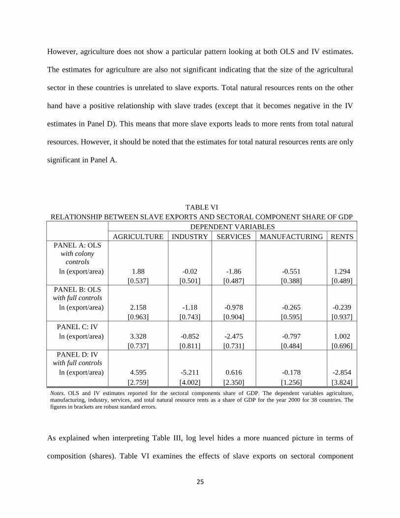
However, agriculture does not show a particular pattern looking at both OLS and IV estimates.

The estimates for agriculture are also not significant indicating that the size of the agricultural

sector in these countries is unrelated to slave exports. Total natural resources rents on the other

hand have a positive relationship with slave trades (except that it becomes negative in the IV

estimates in Panel D). This means that more slave exports leads to more rents from total natural

resources. However, it should be noted that the estimates for total natural resources rents are only

significant in Panel A.

TABLE VI

RELATIONSHIP BETWEEN SLAVE EXPORTS AND SECTORAL COMPONENT SHARE OF GDP

DEPENDENT VARIABLES

AGRICULTURE INDUSTRY SERVICES MANUFACTURING RENTS

PANEL A: OLS

with colony

controls

ln (export/area) 1.88 -0.02 -1.86 -0.551 1.294

[0.537] [0.501] [0.487] [0.388] [0.489]

PANEL B: OLS

with full controls

ln (export/area) 2.158 -1.18 -0.978 -0.265 -0.239

[0.963] [0.743] [0.904] [0.595] [0.937]

PANEL C: IV

ln (export/area) 3.328 -0.852 -2.475 -0.797 1.002

[0.737] [0.811] [0.731] [0.484] [0.696]

PANEL D: IV

with full controls

ln (export/area) 4.595 -5.211 0.616 -0.178 -2.854

[2.759] [4.002] [2.350] [1.256] [3.824]

Notes. OLS and IV estimates reported for the sectoral components share of GDP. The dependent variables agriculture,

manufacturing, industry, services, and total natural resource rents as a share of GDP for the year 2000 for 38 countries. The

figures in brackets are robust standard errors.

As explained when interpreting Table III, log level hides a more nuanced picture in terms of

composition (shares). Table VI examines the effects of slave exports on sectoral component

26

shares of GDP. An interesting finding here is that the effect on the agriculture share in GDP is

positive and significant in all panels with the exception of Panel D (with a p-value of 0.108). So

the share of agriculture in GDP is larger when slave exports increases. Since my argument is that

countries greatly affected by slave exports are less developed today, it follows that countries with

more slaves exported are more agriculture dependent which seems to be the true picture across

African countries. Countries with fewer slave exports, on the other hand, are experiencing

structural transformation explained by Kuznets (1951) as a shift from agriculture to other sectors

(industry and services).

This means that we should also expect a negative relationship between slave exports and the

share of industry and services in GDP. The coefficient for industry remains negative but

insignificant in all panels. The coefficient for services is negative in Panels A to C but becomes

positive in Panel D. However, the estimates are only significant in Panels A (OLS) and C (IV)

but become insignificant when all controls are added in Panels B and D. Manufacturing

estimates are also negative and insignificant like the industry estimates in all panels. Total

resources rents however do not show any particular pattern looking at all panels and the

estimated effect is only significant in Panel A.

27

TABLE VII

RELATIONSHIP BETWEEN SLAVE EXPORTS AND AID (SHARE AND LEVEL)

DEPENDENT VARIABLES

LEVEL SHARE


ln (export/area) -0.009 0.541

[0.046] [0.315]



[0.076] [0.615]

PANEL C: IV


[0.051] [0.365]



[0.139] [1.144]

Notes. OLS and IV estimates reported for net official development assistance in log levels and as a percentage of GNI. The

dependent variable is the share and log level of net ODA for the year 2000 for 38 countries. The figures in brackets are robust

standard errors.

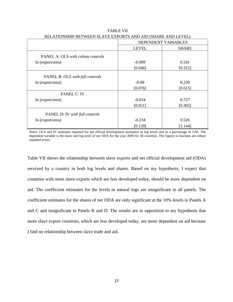
Table VII shows the relationship between slave exports and net official development aid (ODA)

received by a country in both log levels and shares. Based on my hypothesis, I expect that

countries with more slave exports which are less developed today, should be more dependent on

aid. The coefficient estimates for the levels in natural logs are insignificant in all panels. The

coefficient estimates for the shares of net ODA are only significant at the 10% levels in Panels A

and C and insignificant in Panels B and D. The results are in opposition to my hypothesis that

more slave export countries, which are less developed today, are more dependent on aid because

I find no relationship between slave trade and aid.

28

SECTION SIX

CONCLUSION

Combining data from World Bank’s “World Development Indicators’ and Nunn’s “The Long-

Term Effects of Africa’s Slave Trades” (2008), I estimate the impact of Africa’s slave trades on

current development in 38 countries using Nunn’s paper as my major reference. I find a robust

negative and significant relationship between slave exports and current development in the OLS

and IV estimates despite the differences in data source and number of countries used in my paper

compared to Nunn’s.

I estimate regressions with three categories, two of which are made up of different components

of GDP. The first category which consists of household consumption expenditure, government

expenditure and investments is the expenditure components of GDP. I also include variables for

government spending on health and education. The second category is the sectoral components

of GDP and it consists of agriculture, industry and services along with separate variables for

manufacturing and total natural resources rents. The third category consists of only the net

official development assistance (ODA) to a country.

I find three main results supporting the argument that countries that were largely affected by

slave exports are less developed today. Firstly, countries with more slaves exported during the

slave trades spend a smaller share of GDP on government purchases. This is a prediction of the

Wagner’s law which states that the development of a country is accompanied by an increased

share of public spending. I also find weak evidence that public expenditure on health and

education is low which indicates low investment in human capital. Secondly, I find that countries

more affected by slave exports are more agriculture dependent. These countries have not

29

experienced structural transformation defined by Kuznets (1957) as a shift from agriculture to

other sectors (industry and services) of the economy. Lastly, I find no evidence that countries

that experienced more slave exports, which are less developed today, are more dependent on aid

(official development assistance).

30

REFERENCES

Acemoglu, Daron, Simon Johnson and James A. Robinson (2001). “The Colonial Origins

of Comparative Development: An Empirical Investigation.” American Economic Review

91(5), 1369-1401.

Alesina, Alberto, Arnaud Devleeschauwer, William Easterly, Sergio Kurlat and Romain

Wacziarg (2003). “Fractionalization.” Journal of Economic Growth 8(2), 155-194.

Banerjee, Abhijit and Lakshmi Iyer (2005). “History, Institutions, and Economic

Performance: The Legacy of Colonial Land Tenure Systems in India.” American

Economic Review 95(4), 1190-1213.

Duarte, Margarida and Diego Restuccia (2010). “The Role of Structural Transformation

in Aggregate Productivity.” Quarterly Journal of Economics 125, 129-173.

Durevall, Dick and Magnus Henrekson (2011). “The Futile Quest for Grand Explanation

of Long-run Government Expenditure.” Journal of Public Economics 95, 708-722.

Easterly, William and Ross Levine (1997). “Africa’s Growth Tragedy: Policies and

Ethnic Divisions.” Quarterly Journal of Economics 112(4), 1203-1250.

Engerman, Stanley L. and Kenneth L. Sokoloff (1997). “Factor Endowments,

Institutions, and Differential Paths of Growth among New World Economies: A View

from Economic Historians of the United States.” In Stephen Harber, ed., How Latin

America Fell Behind, 260-304.

Engerman, Stanley L. and Kenneth L. Sokoloff (2002). “Factor Endowments, Inequality,

and Paths of Development among New World Economies.” National Bureau of

Economic Research, Working paper 9259.

31

Fenske, James and Namrata Kala (2015). “Climate and the Slave Trade.” Journal of

Development Economics 112, 19-32.

Kongsamut, Piyabha, Sergio Rebelo and Danyang Xie (2001). “Beyond Balanced

Growth.” Review of Economic Studies 68, 869-882.

Kuznets, Simon (1957). “Quantitative aspects of Economic Growth of Nations: II.

Industrial Distribution of National Product and Labour force.” Economic Development

and Cultural Change 5(4), 1-111.

La Porta, Rafael, Florencio Lopez-de-Silanes, Andrei Shleifer and Robert Vishny (1997).

“Legal Determinants of External Finance.” Journal of Finance 52(3), 1131-1150.

La Porta, Rafael, Florencio Lopez-de-Silanes, Andrei Shleifer and Robert Vishny (1998).

“Law and Finance.” Journal of Political Economy 106(6), 1113-1155.

Maddison, Angus (2003). “The World Economy: Historical Statistics.” Organisation for

Economic Co-operation and Development, Paris.

Mohammadi, Hassan, Cak Murat and Cak Demet (2008). “Wagner’s Hypothesis: New

Evidence from Turkey using the Bounds Testing Approach.” Journal of Economic

Studies 35(1), 94-106.

Ngai, L. Rachel and Christopher A. Pissarides (2007). “Structural Change in a

Multisector Model of Growth.” American Economic Review 97(1), 429-443.

Nunn, Nathan (2008). “The Long-Term Effects of Africa’s Slave Trades.” Quarterly

Journal of Economics 123(1), 139-176.

Nunn, Nathan (2009). “The Importance of History for Economic Development.” Annual

Review of Economics 1(1), 65-92.

32

Nunn, Nathan and Leonard Wantchekon (2011). “The Slave Trade and the Origin of

Mistrust in Africa.” American Economic Review 101(7), 3221-3252.

Shelton, A. Cameron (2007). “The Size and Composition of Government Expenditure.”

Journal of Public Economics 91, 2230-2260.

World Bank (2000). World Development Indicators. Retrieved from

http://data.worldbank.org/data-catalog/world-development-indicators

http://data.worldbank.org/data-catalog/world-development-indicators

Slave Trade and Development by Temitope G. Ogunsanmi · Slave Trade and Development by Temitope G....

Documents

Transcript of Slave Trade and Development by Temitope G. Ogunsanmi · Slave Trade and Development by Temitope G....