CHAPTER 3

Characterization of Materials and Loading

There are four kind of materials to be characterized regarding with the topic research. They are subsoil, embankment, geosynthetics, and piles. It is important to know well some properties of them. Because stress and strain relationship in material is induced by loading either static or dynamic loading, the characteristic of loading including magnitude and movement of loading on transportation infrastructure is necessary to be understood.

3.1. Characteristic of Soft Soil in Indonesia

3.1.1 Physical properties

A soil comprises of three basic constituents i.e. solids, liquids and gasses. Solids may be either mineral or organic matter or both with their spaces filled with water and/or air. The soil is saturated when all of pore spaces are filled by water. The purpose of the physical properties testing is to obtained adequate information relating to soil behavior. Some parameters to describe the soil are as follows: water content, Wn, unit weight, , Atterberg limits (LL, PL, PI), sieve analysis, degree of saturation, Sr, organic content, OC.

3.1.1.1. Physical properties of Soft Soil in Java Island

Characteristic of soft soils at some sites in several provinces in Java Island as reported in Development of Guidance for Roadway over Expansive Soil, 2003. Evaluation for this soil is aimed to know characteristic and classification of soil as summarized in Table 3-1.

Table 3-1 Characteristic Soft soils in Java Island

Parameters

Provinces and Link of observed roadCentral Java D.I.Y East Java W. Java

Semarang -Purwodadi

Dempet -Godong

Demak-Kudus

Wirosari-Cepu

Yogya-Wates

Ngawi -Caruban

Surabaya -Gresik

Gresik-Lamongan

Jakarta-Cikampek

1. Unit weigth (gr/cm3)

2. Clay content (%)

3. Liquid limit (%)

4. Plastic Index (%)

5. Linear Shrinkage (%)

6. Water content (%)

7. Passing # 200 (%)

8. Classification of soil

9. Mineral of clay

10.Colour

1.63-1.76

22-43

80-110

52-79

18-22

32-48

83-98

CH, clay

montmorilonite

Browny grey

1.68-1.75

25-40

72-108

40-74

12-26

37-53

82-98

CH,clay

Montmorilonite

browny grey

1.67-1.74

24-34

83-94

44-58

-

29-49

95-98

CH

montmorilo

nite

blackish

grey

1.75 – 1.86

30 - 52

53 -107

24 - 57

-

24 - 40

73 - 96

CH,Silty clay

montmoriloni

te

Greyey black

1.68 – 1.73

30 -52

53 - 107

24 - 97

18

27 -32

76-96

CH, clay

montmoriloni

te

greyey black

1.63-1.89

30-61

72-130

39-79

15-27

40-55

92-98

CH, silty clay

montmoriloni

te, 60 %

Blackish grey

1.61-1.79

23-45

62-90

28-45

-

38-53

89-94

CH,clay

montmorilo

nite 45 %

blackyish

grey

1.73

44

81

48

-

34

97

CH,clay

Montmorilonit

blackish grey

1.59 – 1.71

25 - 58

82 -104

46 - 62

-

34 - 52

92 - 94

MH,Silt

montmorilonite,

10 %

blackish grey

Location : - Depth (m)

- Site (KM)

2.0 -.3.0

36-43

1.0 -3.0

13.8

2.0 -5.0

38.8

1.0 - 4.0

37.5 – 58.25

2.0 – 5.0

23.0 -27.0

1.0 -.4.0

5..0 – 19.0

1.0 -3.0

12.8 – 14.45

1.0 -2.0

16.50

1.0 - 3.0

25.50 – 69.60

Source: Report of Guidance for Roadway over Expansive Soil, 2003

Soft soils are widespread in many locations or regions in Indonesia. In Java Island the soft soils mostly consists of clay and/or silt, whereas in Sumatra and Kalimantan islands they are

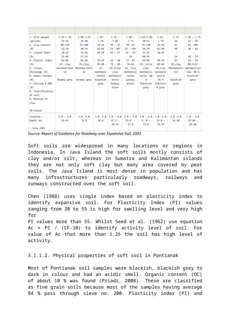
not only soft clay but many area covered by peat soils. The Java Island is most dense in population and has many infrastructures particularly roadways, railways and runways constructed over the soft soil.

Chen (1988) uses single index based on plasticity index to identify expansive soil. For Plasticity Index (PI) values ranging from 20 to 55 is high for swelling level and very high for PI values more than 55. Whilst Seed et al. (1962) use equation Ac = PI / (CF-10) to identify activity level of soil. For value of Ac that more than 1.25 the soil has high level of activity.

3.1.1.2. Physical properties of soft soil in Pontianak

Most of Pontianak soil samples were blackish, blackish grey to dark in colour and had an acidic smell. Organic content (OC) of about 10 % was found (Priadi, 2008). These are classified as fine grain soils because most of the samples having average 84 % pass through sieve no. 200. Plasticity index (PI) and liquid limit (LL) varied widely from 5 to 35 % and 20 to 70 % respectively. According to ASTM standard D2487-00 and USCS based on visually observation, organic content and distribution of grain size, these soils are classified as organic soil. Organic clay deposits seem dominantly near the ground surface. Sandy soil layer is founded 15 to 30 m depth. The water content (Wn) varies widely ranging from 25 to 200 % but decrease with greater depth. Generally, the water content of Pontianak soft organic soil was higher than its liquid limit. Furthermore, a cohesive soil with water content higher than liquid limit is defined as super soft soil clay.

Based on soil investigation for project of Supadio's runway extent (2009) will be complement for data soil in Pontianak. The existing runway 2.250 m long and 30 m wide would be extended 2.600 m long and 45 m wide, respectively. There were 10 sites of taken samples using cone penetrometer test and standard penetration test. As a comparison and supplement that the testing of physical properties for Pontianak soil taken at + 1.5 m depth has also been done in Geotechnical Laboratory TU Bergakademie Freiberg. Furthermore, physical and mechanical properties of soils as described in Table 3-2 below.

Table 3-2 Some subsoil properties at several zones in Pontianak

Parameters Unity

Priadi’s data Project Data of Supadio's runway

Sample of Pontianak soil Design Value

Range of Value Range of Value Range of Value

1. soil classification1. water content, Wn 3. organic content, OC 3. Specific Gravity , Gs4. Unit weight, (kg/m3)5. Liquid Limit, LL6. Plastic Limit, PL 7. Plasticity Index, PI 9. Void Ratio, e 13. Cohesion, c14. Friction angle,10. Compression index, Cc11. Coeff. of compressibility12. Permeability, kv

12. Unconf. Comp. strength13. Oedometer modulus14. Young modulus

-%%-

kN/m3%%%%

kN/m2o--

m/daykN/m2kN/m2kN/m2

Low organic 58.22-169.98

102.2-2.6

12.3-16.4920-7017-355-35

1.02-3.306-16.5

1.0-20.30.16-0.34

-4.4E-6to7.8E-4

--

650-1166

Low organic35 – 91

-2.36 – 2.7013.9 – 18.5

17.10 - 62.46 14.62 – 38.442.48 – 29.670.88 – 2.65

7.2-19.83.03-13.660.278-1.24

1.4E-3 to 7E-3-

8.4-65.5--

Low organic81.6-109.4

11.882.611

13.94-14.3184.52-99.2539.6-50.2234.3-59.6

-0.38-8.08

13.61-27.26------

Low organic85122.6

14.317035352.08

13.70.34

--

24550600

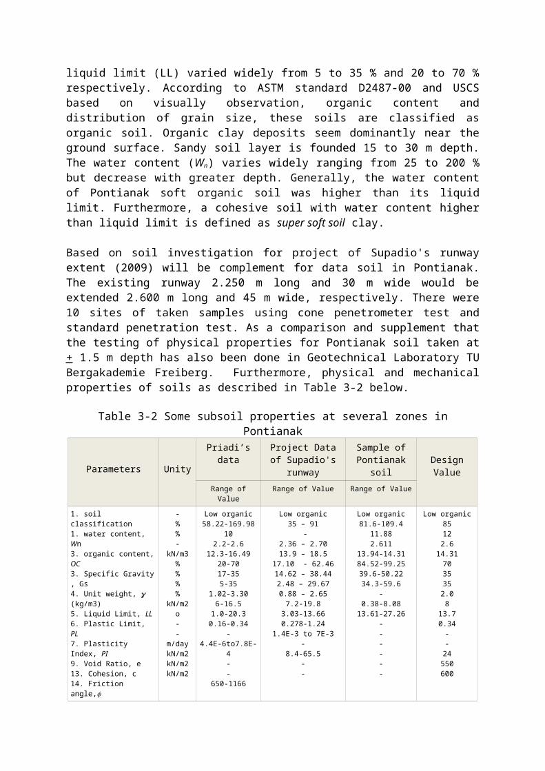
Based on Chen (1988) approach, for soil in this region with PI value average 19.5 can be classified as high for swelling level.

3.1.2. Mechanical properties

Mechanical properties are a necessary thing when investigating strength and deformation of soil during loading. Shear strength of cohesive soil can be determined by using shear tests and/or triaxial tests in which parameters cohesion, c, and internal friction angle, , can be measured. Whilst in predicting the rate of settlement for soil can be carried out by using consolidation test or oedometer testing in other to obtain consolidation index, cc,

3.1.2.1. Direct shear strength characteristic

Normally, specimens of around 20 mm height and 40 cm2 cross-sectional circle surface are utilized in direct shear test, but some problems emerge when doing the kind of test for very soft material. A little adjustment is an important thing in this case based on previous experiences which the height of specimen needs to be higher than in the normal situation. For consolidated drained (CD) shear test, height of specimen around 30 mm was mounted to overcome the high compressibility of soil in other to avoid friction between upper and lower ribs in the shear box. For consolidated drained shear tests were conducted with normal stresses 50, 75, 100, 150, 200 kN/m2 respectively and consolidation time set up for 2 days before running shearing tests.

3.1.2.2. Compression characteristic

When soils undergo a loading, because of their relatively low permeability, their compression is controlled by the rate at which water is squeezed out of the pores. The slope e against log ’ plotted for normally consolidated soil is referred to as compression index, cc. The load increment ratio was uniform where the loading was from 25 kN/m2 to 800 kN/m2. The compression index, cc, varies widely with the increasing depth, however, the depth does not influence of cc.

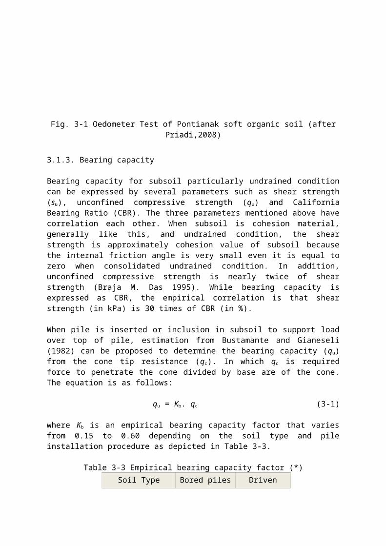
Priadi (2008) characterized the Pontianak soft organic soil compressibility behavior that the top layer (around 10 m deep) is highly compressible ranging from 0.5 to 1.38 with an average value of about 0.8, whereas at below this layer ranging from 0.2 to 0.5 with an average value is about 0.3. Meanwhile, the recompression index, cs, ranges widely from 0.03 to 0.25. Some of the 1-D Oedometer test results are shown in Fig. 3-1.

The over consolidated ratio, OCR, is defined as the ratio between the pre-consolidation stress and the effective in-situ stress. OCR is a state parameter that indicates the amount of over-consolidation of the soil (Brinkgreve,2001). This value notably reduces with a depth. Pontianak soft organic soil are heavily over consolidated from ground surface to about of 5 m depth due to the wetting and drying cycles during deposition. The over consolidation ratio ranges from 2 to 11 at this layer, whereas OCR values range from 1.3 to 2 are found at 5 to 20 m depth.

Fig. 3-1 Oedometer Test of Pontianak soft organic soil (after Priadi,2008)

3.1.3. Bearing capacity

Bearing capacity for subsoil particularly undrained condition can be expressed by several parameters such as shear strength (su), unconfined compressive strength (qu) and California Bearing Ratio (CBR). The three parameters mentioned above have correlation each other. When subsoil is cohesion material, generally like this, and undrained condition, the shear strength is approximately cohesion value of subsoil because the internal friction angle is very small even it is equal to zero when consolidated undrained condition. In addition, unconfined compressive strength is nearly twice of shear strength (Braja M. Das 1995). While bearing capacity is expressed as CBR, the empirical correlation is that shear strength (in kPa) is 30 times of CBR (in %).

When pile is inserted or inclusion in subsoil to support load over top of pile, estimation from Bustamante and Gianeseli (1982) can be proposed to determine the bearing capacity (qu) from the cone tip resistance (qc). In which qc is required force to penetrate the cone divided by base are of the cone. The equation is as follows:

qu = Kb. qc (3-1)

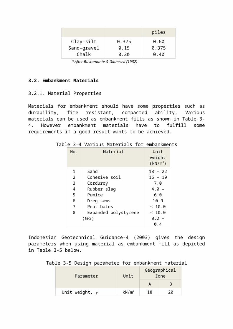
where Kb is an empirical bearing capacity factor that varies from 0.15 to 0.60 depending on the soil type and pile installation procedure as depicted in Table 3-3.

Table 3-3 Empirical bearing capacity factor (*)Soil Type Bored piles Driven piles

Clay-siltSand-gravel

Chalk

0.3750.150.20

0.600.3750.40

*After Bustamante & Gianeseli (1982)

3.2. Embankment Materials

3.2.1. Material Properties

Materials for embankment should have some properties such as durability, fire resistant, compacted ability. Various materials can be used as embankment fills as shown in Table 3-4. However embankment materials have to fulfill some requirements if a good result wants to be achieved.

Table 3-4 Various Materials for embankmentsNo. Material Unit weight

(kN/m3)

12345678

Sand Cohesive soil Corduroy Rubber slag Pumice Dreg saws Peat bales Expanded polystyrene (EPS)

18 – 2216 – 19

7.04.0 – 6.0

10.9< 10.0< 10.0

0.2 – 0.4

Indonesian Geotechnical Guidance-4 (2003) gives the design parameters when using material as embankment fill as depicted in Table 3-5 below.

Table 3-5 Design parameter for embankment material

Parameter UnitGeographical Zone

A B

Unit weight, Undrained shear strength, Su

Cohesion, C ' Internal friction angle, '

kN/m3

kN/m2

kN/m2

[ O ]

181001035

201005

30Source: Indonesian Geotechnical Guidance-4(2003)

A Java island (vulcanic rocks)B Sumatra, Kalimantan, Sulawesi. Papua island (sedimentary and metamorphic rocks)

3.2.2 Strength of material

As illustrated in Table 3-4 above, the higher value for unit weight,, internal friction angle, and shear strength, su, will give a good result regarding with soil arching on embankment. Usually, embankment fill is a cohesionless material or very small of cohesion value.

3.2.3. Maximum Height of embankments

Stability for maximum or critical height of embankments without ground treatment can be calculated using equation below:

Hc = 4 cu / (3-2)

where is unit weight of embankment fill and cu is the undrained shear strength of subsoil beneath embankments.

3.2.4. Dynamic Properties

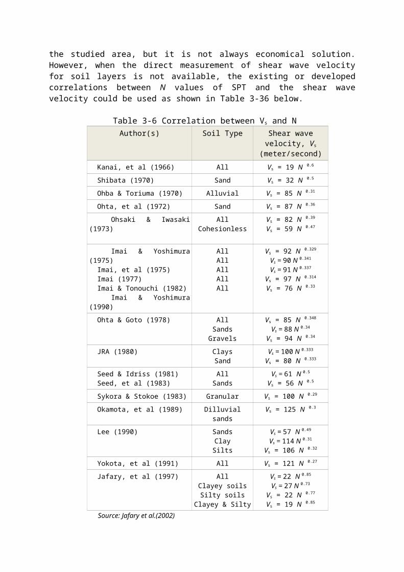
Shear modulus, damping ratio and shear wave velocity profiles are an important input parameters in site response analysis. Jafari, M.K. et al. (2002), based on field geoseismic investigation data for fine grained soil in Tehran, present new correlation for Shear-wave (Vs) and Number of blows (N) from Standard penetration test (SPT). Some researchers also give some equations for the correlation between Vs and N.

Although shear wave velocity could be obtained directly from filed investigation or laboratory testing of soil samples of the studied area, but it is not always economical solution. However, when the direct measurement of shear wave velocity for soil layers is not available, the existing or developed correlations between N values of SPT and the shear wave velocity could be used as shown in Table 3-36 below.

Table 3-6 Correlation between Vs and NAuthor(s) Soil Type Shear wave velocity, Vs

(meter/second) Kanai, et al (1966) All Vs = 19 N 0.6

Shibata (1970) Sand Vs = 32 N 0.5

Ohba & Toriuma (1970) Alluvial Vs = 85 N 0.31

Ohta, et al (1972) Sand Vs = 87 N 0.36

Ohsaki & Iwasaki (1973) AllCohesionless

Vs = 82 N 0.39

Vs = 59 N 0.47

Imai & Yoshimura (1975) Imai, et al (1975) Imai (1977) Imai & Tonouchi (1982) Imai & Yoshimura (1990)

AllAllAllAllAll

Vs = 92 N 0.329

Vs = 90 N 0.341

Vs = 91 N 0.337

Vs = 97 N 0.314

Vs = 76 N 0.33

Ohta & Goto (1978) AllSands

Gravels

Vs = 85 N 0.348

Vs = 88 N 0.34

Vs = 94 N 0.34

JRA (1980) ClaysSand

Vs = 100 N 0.333

Vs = 80 N 0.333

Seed & Idriss (1981) Seed, et al (1983)

AllSands

Vs = 61 N 0.5

Vs = 56 N 0.5

Sykora & Stokoe (1983) Granular Vs = 100 N 0.29

Okamota, et al (1989) Dilluvial sands Vs = 125 N 0.3

Lee (1990) SandsClaySilts

Vs = 57 N 0.49

Vs = 114 N 0.31

Vs = 106 N 0.32

Yokota, et al (1991) All Vs = 121 N 0.27

Jafary, et al (1997) AllClayey soilsSilty soils

Clayey & Silty

Vs = 22 N 0.85

Vs = 27 N 0.73

Vs = 22 N 0.77

Vs = 19 N 0.85

Source: Jafary et al.(2002)

Once shear wave velocity is determined, and then shear modulus of material, G, is obtained using equation G= .Vs

2, which is density of soil.

The behaviour of soil under cyclic loading is non-linear and dependent on some factors including soil type, confining pressure, number of loading cycles and amplitude of loading. Non linear hysteretic soil behaviour is commonly characterized by a viscous damping and equivalent shear modulus (Seed and Idriss, 1970; Hardin and Drenevich, 1972). Damping is a measure of energy dissipation and it increase with increasing magnitude of cyclic shear strain, whereas Shear modulus decrease with increasing magnitude of cyclic shear strain. It is also known that dynamic properties of soil are influenced by plasticity index, void ratio, relative density and number of cycles (Cabalar and Cevik, 2008).

Shear modulus of air dry clean sands at certain level of shear strain can be represented approximately by the following empirical equation irrespectively of kinds of sands.

( = 10-6) G = 900 (2.17−e)2

1+e p0.38 (3-3)

( = 10-5) G = 850 (2.17−e)2

1+e p0.44 (3-4)

( = 10-4) G = 700 (2.17−e)2

1+e p0.50 (3-5)

Where G is shear modulus in kg/cm2, p is mean principle stress in kg/cm2 and e is void ratio. Eq. 3-5 is identical to the empirical equation for round Ottawa-sand proposed by Hardin, et al. (1972).

All tests demonstrated the well known dependence of Gmax on effective confining pressure 'o

and density expressed in terms of the void ratio e. In other to an analytical expression for the Gmax = Gmax ('o) relationship, the general equation suggested by Hardin (1972) is adopted.

Gmax = s

0.3+0.7 e2 pa1-n ( ’o) n (3-6)

Where: S is a stiffness coefficient. The experimental results are closely approximated by setting S= 420 and n= 0.6. It should be noticed that the value of the exponent n is higher than widely used for cohesive and cohesiveless soils which ranges between 0.4 and 0.5. The variation of shear modulus with shear strain amplitude as expressed in the following equation.

G = Gmax / (1 + 200 ) (3-7)

The damping ratio D was found to be essentially independent on confining pressure and density. An average value Dmin=2% was determined from all tests. The increase of damping with shear strain amplitude may be approximately expressed by:

D/Dmin=1+ A

1+α /¿¿ (3-8)

with A = 6.2 and = 6.5.10-4.

The soil starts to exhibit hysteretic and non-linear behaviour in the shear strain range between 10-6 and 10-3, where the secant stiffness decreases with the increasing of the strain level. Various authors have suggested several equations to connect the damping ratio and the shear modulus when both ate functions of shear strain. Hardin and Drnevich (1972) derived the simple relationship equation.

D = Dmax [1 – G/Go ] (3-9)

Where: G is the secant modulus and Go is the initial shear modulus.

Park and Stewart (1980) have proposed an equation for sandy soils and separate equation for clayey soil respectively.

For sandy soils D = 32.85 [0.54 (G/Go)2 – 1.53 (G/Go) +1] (3-10)For clayey soils D = 17.83 [0.56 (G/Go)2 – 1.39 (G/Go) +1] (3-11)

3.3. Geosynthetics

3.3.1. Material Properties

The geosynthetics terminology may be based on the subdivision by prEN ISO 10318. According to this standard “Geosynthetics” is a generic term describing a product at least one of whose components is made from a synthetic or natural polymer, in the form of a sheet, a strip or a three dimensional structure, used in contact with soil and/or other materials in geotechnical and civil engineering applications. As depicted in Fig. 3-2 below that geosynthetics can be differentiated into permeable and impermeable products.

Fig. 3-2 Geosynthetics subdivision (after prEN ISO 10318)

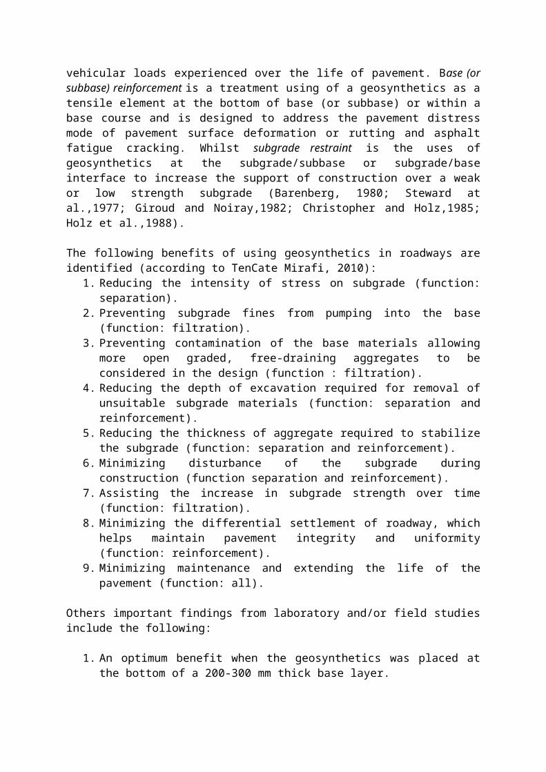
The use of a geosynthetics in pavement system reinforcement is to aid in support of traffic load. Traffic loads may be vehicular loads experienced over the life of pavement. Base (or

subbase) reinforcement is a treatment using of a geosynthetics as a tensile element at the bottom of base (or subbase) or within a base course and is designed to address the pavement distress mode of pavement surface deformation or rutting and asphalt fatigue cracking. Whilst subgrade restraint is the uses of geosynthetics at the subgrade/subbase or subgrade/base interface to increase the support of construction over a weak or low strength subgrade (Barenberg, 1980; Steward at al.,1977; Giroud and Noiray,1982; Christopher and Holz,1985; Holz et al.,1988).

The following benefits of using geosynthetics in roadways are identified (according to TenCate Mirafi, 2010):

1. Reducing the intensity of stress on subgrade (function: separation).2. Preventing subgrade fines from pumping into the base (function: filtration).3. Preventing contamination of the base materials allowing more open graded, free-

draining aggregates to be considered in the design (function : filtration).4. Reducing the depth of excavation required for removal of unsuitable subgrade

materials (function: separation and reinforcement).5. Reducing the thickness of aggregate required to stabilize the subgrade (function:

separation and reinforcement).6. Minimizing disturbance of the subgrade during construction (function separation and

reinforcement).7. Assisting the increase in subgrade strength over time (function: filtration).8. Minimizing the differential settlement of roadway, which helps maintain pavement

integrity and uniformity (function: reinforcement).9. Minimizing maintenance and extending the life of the pavement (function: all).

Others important findings from laboratory and/or field studies include the following:

1. An optimum benefit when the geosynthetics was placed at the bottom of a 200-300 mm thick base layer.

2. For thicker base sections, the most beneficial reinforcement location appeared to be in the middle of the base, where geogrids were found to perform best.

3. For thin bases (less than 200 mm), lack of separation was noted as potential problem for geogrids. Geogrid-geotextile composites tend to perform better for thin bases, especially where subgrade strengths were below a CBR of 3.

4. Reinforcement benefits were observed with subgrade strengths up to a CBR of 8.

The benefits using geosynthetics as reinforcement can be defined by TBR (Traffic benefit ratio) and BCR (Base course reduction). TBR is defined as the ratio of number of cycles necessary to reach the same rut depth for a test section containing reinforcement to unreinforced section with the same section thickness and subgrade properties. Furthermore, BCR is expressed as a percentage savings of the unreinforced base course thickness.

Table 3-7 Summary of laboratory and field test sections (TenCate Mirafi,2010)Material TBR BCR

Geotextiles :Range

Typical value1 – 2201.5 – 10

22 – 33 %

Geogrids :Range 0.8 – 670 30 – 50 %

Surface course

Base course

Surface course

Base course

Surface course

Base course

Surface course

Base course

Typical value 1.5 – 70

Besides the ratio coefficients (TBR, BCR), the following properties are considered to influence performance : tensile strength at 1%, 2% and 5% strain, coefficients of pullout and direct shear, aperture size (grids) and percent open area (geotextiles) and stiffness properties including the flexural rigidity and aperture stability. For subgrade restraint applications, the properties of tensile strength at 2% and 5% strain are primarily related to geosynthetics performance.

3.3.2. Position of Geosynthetisc in Pavement Design Practice

There are three general applications for the use of geosynthetisc reinforcement in pavements. Therefore, the appropriate application with the ultimate objective of maximizing performance as the following guidance for these three distinct applications:

1. Weak Subgrade (CBR < 3), For Thin (< 250 mm) Base Sections and Thick (> 250 mm) Base Sections.

When a weak subgrade exists, woven geotextile should be placed at the surface interface. In addition, if the required base course is greater than 250 mm (10 in), a second layer of reinforcement, biaxial geogrid, should be placed in the middle of the base course section.

2. Firm Subgrade (CBR > 3), For Thin (< 250 mm) Base Sections and Thick (> 250 mm) Base Sections.

For a firm subgrade and relatively thin base course section is designed biaxial geogrid at the subgrade interface. While geogrid can be placed in the middle of the base course when firm subgrade and relatively thick base course section is designed.

(a) Weak Subgrade, Base Course < 250 mm (b) Weak Subgrade, Base course > 250 mm

Geogrid Geotextile Geotextile

/////// Subgrade ////////// /////// Subgrade //////////

(c) Firm Subgrade, Base Course < 250 mm (d) Firm Subgrade, Base course > 250 mm

Geogrid Geogrid

/////// Subgrade ////////// /////// Subgrade //////////

Fig. 3-3 Positions of geosynthetics in pavement design practice (after TenCate Mirafi,2010)

3.3.3. Tensile Strength of Geosynthetics

Tensile strength of geosynthetics depend on row material of geosynthetic such as aramid or polyamide (PA), polyethylene of High density (PE-HD), polyester (PET), polypropylene (PP) and polyvinyl alcohol (PVA). Range of tensile strength from various raw materials of geosynthetics is as shown in Fig. 3-4 below.

(a) (b)

Fig. 3-4 Typical strain-force behaviour of reinforcement (a) Exxon,1989 (b) Carlson,1987

Typical short term strength of geosynthetics is as described in Table 3-8 for various raw materials (EBGEO,2010, Althoff,2011)

Table 3-8 Tensile strengths of geosynthetics (after Althoff ,2011; EBGEO 2010)

Raw material

Product TypeTypical short term strengths

[kN/m]Typical elongation at

failure [%]

from to max. from to

AR Woven and GeogridsWoven Geotextile

40100

12001400

2200300

22

44

PE Woven and GeogridsExtruded geogridsWoven Geotextile

204030

150150200

300200400

151015

201520

PET Woven and GeogridsBonded geogridsWoven Geotextile

2020

100

800400

1000

12005001600

868

151015

PP Woven and GeogridsBonded GeogridsExtruded geogridsWoven Geotextile

20202020

20020050200

500400

-600

8888

15152020

PVA Woven and GeogridWoven Geotextile

3030

1000900

16001800

44

55

When choosing geosynthetics for reinforcement, there are two factors that must be considered well namely internal and external factor. Internal factors such as tensile strength, creep properties, whereas external factors such as kind of embankment fill, endurance against environment (ultra violet, acidic or alkaline matter, micro organism. In other to cover all conditions, strength of geosynthetics has to be adjusted using some partial factors.

Table 3-9 Conversion factors of geosynyhetic reinforcements (Nordich Guidance,2003)Conversion parameters Conversion factor

Creep factorInstallation damage

Biological and chemical degradation

Table 3-10 Conversion factors for long term properties (Nordich Guidance ,2003)Conversion parameters Conversion factor, Material factor, fm

Steel Polyester (PET) Polypropylene (PP) Polyamide (PA) Polyethylene (PE)

0.80.40.2

0.350.2

1.252.55

2.85

Table 3-11 Conversion factors for damage during installation (Nordich Guidance ,2003)Conversion parameters Conversion factor, Material factor, fd

Clay/silt Sand Gravel (Natural) Gravel (Broken) Chrused Rockfill

0.910.830.770.720.67

1.11.21.31.41.5

The material factor for biological and chemical degradation, fenv , may according to Swedish Road administration publication 1992:10 be assumed 1.1 as long as the pH value ranges between 4 and 9, which gives a conversion factor of = 0.91.

Allowable tensile strength of geosynthetics for reinforcement design is defined as ultimate tensile strength divided by reduction factor (or partial factor).

a = u {1/fd, 1/fenv,1/fm,1/fc} (3-12)

Where:a = allowable strengthu = ultimate strengthfd = partial factor for mechanical damagefenv = partial factor for environmentfm = partial factor for extrapolation of tensile strengthfc = partial factor for construction safe

3.4. Characteristic of Piles

There are three classifications of columnar foundation include (Han and Wayne,2000) namely :

flexible column (such as stone columns and lime columns) semi-rigid columns (such as lime-cement and soil-cement columns) rigid piles (such as concrete pile, timber piles, and vibro-concrete piles)

3.4.1. Wooden Pile

Strength of wood can be grouped into four classes of strength and type of stress as in Table 3xx (Indonesian Wooden Construction Code, 1971). Wooden material with class 1 and 2 are usually used in construction demand.

Table 3-12 Strength class for wooden materialNo. Type of stress Strength class of wood (kg/cm2)

1 2 3 4

1 flexural 150 100 75 50

2 comp or tensile 130 85 60 45

3 compressive 40 25 15 10

4 20 12 8 5

5 Young Modulus, E (kg/cm2) 125000 100000 80000 60000

According to new code SNI 2002 (Indonesian National Standardization,2002), quality of wooden material or quality code use mixed Letter and Number to declare Elasticity Modulus as in Table 3-13 below.

Table 3-13 Quality code for wooden materialCode of Quality

Young Modulus

[MPa]

Flexural Strength

Fb

[MPa]

Tensile strength parallel fiber

Ft

[MPa]

Tenslie strength perpendic. fiber

Fc

[MPa]

Shear strength

Fv

[MPa]

Compr. Strength perpendic.

Fc

[MPa]

E26E25E24E23E22E21E20E19E18E17E16E15E14E13E12E11

25000240002300022000210002000019000180001700016000150001400013000120001100010000

66625956545047444238353230272320

60585653504744423936333128252219

46454543414039373534333130282725

6.66.56.46.26.15.95.85.65.45.45.25.14.94.84.64.5

24232221201918171615141312111110

E10 9000 18 17 24 4.3 9

Elasticity modulus or Young modulus of wooden material can be estimated using equation below (SNI Kayu, 2002).

E (Mpa) = 16,000 G 0.7 (3-13)

Where: G is specific gravity of wooden material at water content 15 %.

3.4.2. Concrete Pile

It is similar to wooden material that for cementitious pile (or concrete pile) Young modulus is important parameter. Cemented material as concrete column is subjected to high compressibility stress. Young modulus can be estimated using compressive strength of concrete.

Ec = 14850 fc' 0.5 (kg/cm2) (3-14)

Relationship between characteristic compressive strength and flexural strength as described in Eq. 3-15 below.

fcf = K. fc' 0.5 (Mpa) (3-15)

or fcf = 1.13 K. fc' 0.5 (kg/cm2) (3-16)

where: Ec = Young modulus of concretefc' = characteristic compressive strength 28 dayfcf = flexural-tensile strength 28 dayK = 0.7 for gravel and 0.75 for crushed stone

3.4.3. Stone Column

Hughes and Withers (1974) performed pioneering laboratory studies of sand columns within a cylindrical chamber containing clay and used radiography to track the deformations occurring within and outside the columns. They found that CCET (cylindrical cavity expansion theory) represented the measured column behaviour very well and proposed that the ultimate vertical stress (q) in a stone column could be predicted by:

q = 1−sin ’1−sin ’ ( ’ro + 4c ) (3-17)

where: ' is the friction angle of stone infill, 'ro is the free-field lateral effective stress and c is the undrained shear strength.

The equation above is widely used in practice today. There are alternative approaches for estimating the bearing capacity of single column and column group, such as that recently published by Etezad et al. (2006). The authors report an analytical treatment of bearing capacity failure mechanisms. The failure mechanisms adopted are based upon the output from a combination of finite element analysis and field trials.

Absolute and differential settlement restrictions usually govern the length and spacing of columns, and the preferred method of estimating post-treatment in European practice was

developed by Priebe (1995). Although this method is strictly applicable to infinite array of columns and has some empiricism in its development.

Priebe's settlement improvement factor, n, defined as:

n = settlement without treatment / settlement with treatment (3-18)

is a function of the friction angle of stone ' , the soil's Poisson's ratio and an area replacement ratio dictated by the column spacing. The area replacement ratio is defined as Ac/A , where Ac = cross-sectional area of one column and A = total cross-sectional area of the 'unit cell' attributed to each column. Ac/A is related geometrically to the column radius, r, and column spacing, s, according to:

Ac/A = k (rs )2 (3-19)

Where: k is and 2/√3 for square and triangular column grids respectively.

Fig. 3-5 Typical of column arrangements, triangular and square grid

Priebe's ' basic improvement factor ' may be derived from the chart shown in Fig. 3-6 below. Need to be note that the reciprocal area replacement ratio A/Ac is used on the chart.

Fig. 3-6 Priebe's basic improvement factor (after Priebe,1995)

A lower limit to the undrained strength of cu = 15 kPa is suggested for treatment with stone column, although there have been situations where softer soils have been successfully improved (Raju et al.,2004). In other hand UK National House Building Council

(NHBC,1988) suggests that stone columns should not be used when Ip > 40 %. Muir Wood et al,(2002) conducted what is considered to be the most comprehensive laboratory model investigations of large groups of columns. The results suggest that significant improvement to bearing capacity requires an area replacement ratio of 25 % or greater.

McKelvey et al. (2004) used a transparent medium with “clay-like” properties to allow visual monitoring of the columns throughout foundation loading. The main findings of this research relate to optimum column aspect ratio L/d (L=column length, d=column diameter) that in the case of “short column” (i.e. L/d=6), bulging took place over the entire length of column. The “long column” (L/d=10) deformed significantly in the upper region whereas the bottom portion remained undeformed. McKelvey et al. (2004) postulated a “critical column length” of L/d=6, which is in keeping with earlier work (Hughes and Withers,1974; Muir Wood et al. 2004).

3.4.4. Soil Cement Column

The deep mixing method is a technology that mixes in-situ soils with cementitious materials to form a vertical stiff inclusion in the ground. The deep mixing method (DMM) utilizes quicklime, slaked lime, cement, fly ash, and/or other agents. The agents, widely referred to as “binders”, may be introduced in the form of either a dry powder or slurry.

In the late 1960's, Japan and Sweden independently began research and development of deep soil mixing techniques using granular quicklime. The Japanese were focusing on soil improvement techniques suited to large marine and estuarine projects, while Sweden was primary focusing on soil improvement of soft clays for road and railway projects. The method in which dry powdered lime and cement are used as the stabilizing agents is generally known as the “Dry Method of Deep Mixing”, whereas the use of stabilizing agents in slurry form referred to as the “Wet Method of Deep Mixing” by the mid 1970's, in effort to improve the uniformity of soil treated by deep mixing. Typical operating parameters of the Japanese mixing machines are summarized in Table 3-14.

Table 3-14. Typical Japanese mixing installation parameters (after Kaiqiu,2000)Description Single drive shaft Doble drive shaft Multibarrel drive shaft

Depth of stabilization 49 ft (15 m) > 49 ft (15 m) 98-131 ft (30 - 40 m)

Penetration velocity 2 - 3.3 ft/m0.6 - 1.0 m/min

0.7 - 3.3 ft/m0.2 - 1.0 m/min

3.3 - 6.6 ft/m1.0 - 2.0 m/min

Withdrawal velocity 2 - 3.3 ft/m0.6 - 1.0 m/min

0.7 - 3.3 ft/m0.2 - 1.0 m/min

3.3 - 6.0 ft/m1.0 - 1.5 m/min

Rotating speed 50 rpm 46 rpm 20 - 30 rpm (penetration)40 - 60 rpm (withdrawal)

Deep mixing methods in the U.S. have been used on several projects either dry or wet method. In general, dry mixed stabilization is appropriate for sites with relatively deep deposits of very soft soil, and sufficient groundwater to hydrate both the lime and the cement (Esrig and MacKenna,1999). Cohesive soils with moisture contents between 60 and 200 % are best suited for dry mixing.

While several different types of laboratory tests are used to evaluate the shear strength and stiffness of deep mixed columns, the most frequently used is the unconfined compression test,

mainly because of the simplicity of the test. Many factors affect the unconfined compressive strength because of a wide variety of soil types and binder mixes. The 28-day unconfined compressive strength for soil treated by the wet method may range from 140 to 27000 kPa (Haley&Aldrich,2000; Kaiqiu,2000; Tatsuoka&Kobayashi,1983) whereas using the dry method range from 14 to 2700 kPa (Hebib&Farrell,2002; Jacobson et al, 2002;Kaiqiu,2000). Unconfined compressive strength, qu, for three projects in U.S. are presented in Table 3-15.

Table 3-15 Specified value of qu on deep mixing projects in the USProject Soil type / binder

amountSpecified qu Reference(s)

Oakland Airport Roadway, California

Wet method; Loose sandy fill and soft soil; 160-240 kg/m3 cement

At 28 days, Average qu > 1035 kPa, Minimum qu > 690 kPa

Yang et al,2001

Central Artery Project, Boston

Wet method; Fill and organic soft clay; 220-300 kg/m3 cement

At 56 days, Maximum qu > 26900 kPa, Minimum qu > 2100 kPa

Lambrechts et al,1998; Maswoswe,2001

I-95 Route 1,Alexandria

Wet method; Soft organic clay; 300 kg/m3 cement

At 28 days, Average qu > 1100 kPa, Minimum qu > 690 kPa

Shiells et al,2003;Lambrechts et al,1998

Source, Smith, 2008

Stabilization of soft organic soils with cement columns using the mix-in-place technique (MIP) for a railway embankment at the section Büchen-Hamburg was upgrade in 2003 by the German Railway company (Deutsche Bahn) to allow a train speed of 230 km/h (Schwarz&Raithel,2005). The cement columns (diameter 0.63 m and 5-8 m length) were installed in a square 1.5x1.5 m grid, containing 2.5 to 3 % cement, which can be characterized as a wet deep mixing technique, the composition of binder (water, cement and bentonite) and the water binder ratio (approx. 1.0). Per 500 m3 of treated soil, 6 unconfined compression tests were carried out after 28 days. According to the test, unconfined compressive strength after 28 days of all sample exceed the design criteria of qu > 2.2 Mpa.

For cement columns installed by the wet method, Takenaka (1995) reports that undrained shear strength is equal to one-half of the unconfined compressive strength for those values below several hundred kPa and become less than one-half when they are greater than several hundred kPa. As a rule of thumb, Tanaka (1995) recommends that undrained shear strength be taken as one-third of the unconfined compressive strength. Kivelo (1997) found that the undrained shear strength can be less than one-half the unconfined compressive strength at low confining pressures. However, when the total confining pressure exceeds 150-250 kPa, the undrained shear strength becomes almost constant at a value equal to one half of the unconfined compressive strength.

Fig. 3-7 Undrained shear strength of lime/cement column (after Kivelo,1997)

The peak strength is typically reached at strains 0f 1% to 2% and decrease in strength once the peak strength is exceeded (Kivelo,1998). The residual strength of soil-cement is 65% to 90% of the unconfined compressive strength (Tatsuoka&Kobayashi,1983).

The undrained secant modulus of elasticity, E50, which evaluated at 50 % of the peak strength is a measure of soil-cement compressibility. Some researchers correlate E50 to unconfined compressive strength for columns installed the dray method (Braker,2000; Broms, 2003; Jacobson et al., 2003; Navin&Filz, 2005). Whilst for cement treated soils using the wet method also have been performed and give relatively higher values of secant modulus of elasticity than those using the dry method (Kawasaki et al. 1981, Navin&Filz 2005,Fang et al. 2001). The relationship between E50 and qu is provided in Table 3-16.

Table 3-16 Relationship E50 and qu

Binder type E50 Reference(s)

Dry lime/cement 50 – 180 qu

75 qu

Baker,2000; Broms,2003 Jacobson et al. 2003

Dry cement 65 – 250 qu

300 qu

Baker,2000; Broms,2003 Navin and Filz,2005

Wet cement350 – 1000 qu

30 – 300 qu

150 qu

300 qu

Kawasaki et al,1981 Fang et al,2001 McGinn and O'Rouke,2003Navin and Filz,2005

Cited M. Smith.2008

When the modulus of elasticity is used in design analysis, the secant modulus E50 is typically used as the design value of column Ecol. The modulus of elasticity on samples prepared in the laboratory is typically higher than modulus determined from coring test obtained in situ actual columns (Broms, 2003).

The oedometer compression modulus Eoed is related to modulus of elasticity Ecol and Poisson's ratio as follows:

Eoed = Ecol (1-) / (1+) (1- 2 ) (3-20)

Generally the Poisson's ratio of deep mixed treated soil is around 0.25 to 0.45 (Terashi, 2003). Therefore, Eoed is equal to 1.2 to 3 Ecol.

The total unit weight of treated soil using the dry method increase by 3% to 15% above that of the untreated soil. Whilst tensile strength of soil improved by the wet method, it is 10% to 20% of unconfined compressive strength. Moreover, permeability of treated soil in range 10-7

to 10-8 m/s is routinely achievable.

3.5. Characteristic of Loading

Transportation infrastructure such as roadway, railway and runway is mainly subjected by moving load. Although for certain situation they are static loading such as car parking at parking load, aircraft parking on parking stand at the apron.

3.5.1. Vehicular Traffic

For vehicles crossing on the roadway, all kind of vehicles refer to Equivalent Single Axle Load (ESAL) 18 kips (or 8.12 ton) with inflation pressure 80 psi (560 kPa). Wheel configuration may be single, dual wheels and tandem. For light vehicles (passenger cars) have an inflation pressure around 32 psi (225 kPa).

3.5.2. Airplane

It is a little higher load on the runway which loading coming from aircraft depends on weight, tire pressure, wheel configuration (single, dual, tandem) of airplane. Tire pressures of airplanes vary from 0.5 MPa to more than 1.5 MPa.

In other to accommodate the various airplanes demand for operational movement, it needs to provide aerodrome areal as shown in Table 3-17. The aerodrome reference code uses number and letter codes to express class of airport (ICAO, 1999).

Table 3-17 Aerodrome reference code (ICAO, 1999)Code element 1 Code element 2

Code number

Aeroplane reference field length

Code letter

Wingspan Outer main gear wheel span *

[1] [2] [3] [4] [5]

1 Less than 800 m A Up to but not including 15 m

Up to but not including 4.5 m

2 800 m up to but not including 1200 m

B 15 m up to but not including 24 m

15 m up to but not including 24 m

3 1200 m up to but not including 1800 m

C 24 m up to but not including 36 m

6 m up to but not including 9 m

4 1800 m and over D 36 m up to but not including 52 m

9 m up to but not including 14 m

E 52 m up to but not including 65 m

9 m up to but not including 14 m

F 65 m up to but not 14 m up to but not

including 80 m including 16 m* Distance between the outside edges of the main gear wheels.

Maximum allowable tire pressure category consists of High (no pressure limit), Medium (pressure limited to 1.50 MPa), Low (pressure limited to 1.00 Mpa) and Very low (pressure limited to 0.50 MPa. The higher tire pressure indicates the heavier weight of airplane.

3.5.3. Trains

In Germany, according to Ril 836 for rail infrastructure, the subgrade or improved subgrade has to support a load above this surface layer at least around 52 kPa as described in Fig. 3-8. For high speed trains from 100 to 300 km/h, it needs the additional layer around 1 to 2 times of the superstructure thickness (Muncke et al., 1999; Kempfert et al., 1999).

Fig. 3-8 Cross section for rail track (after Ril 836)

It is different for each country for the standard axle load. For instance in Greece, Beskou et al. (2011) reported that for locomotive (or engine) is around 210 kN and 150 kN for carriage. In Indonesia, railway infrastructure is subjected to axle load maximum 180 kN (Indonesian Railway Code, 2003).

.