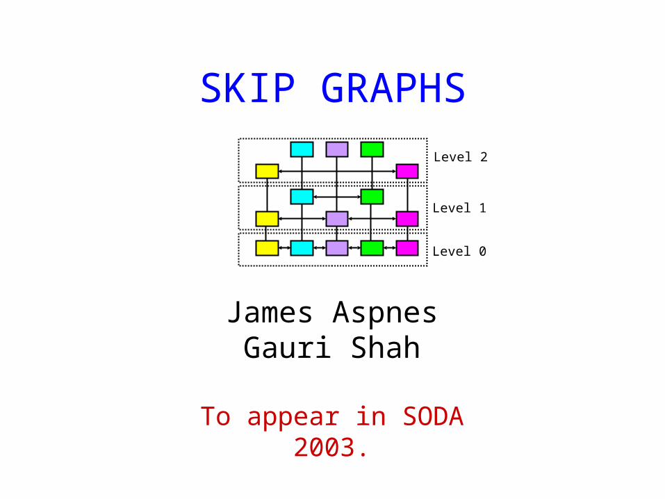
SKIP GRAPHS

James AspnesGauri Shah

To appear in SODA 2003.

Level 0

Level 1

Level 2

2

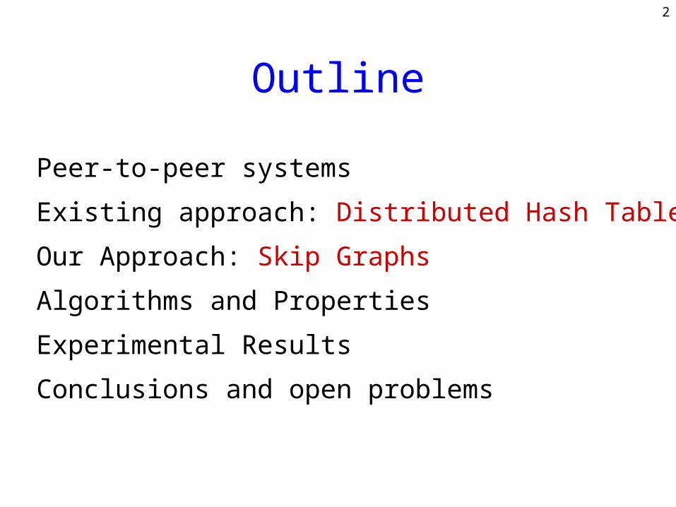
Outline

• Peer-to-peer systems

• Existing approach: Distributed Hash Tables

• Our Approach: Skip Graphs

• Algorithms and Properties

• Experimental Results

• Conclusions and open problems

3

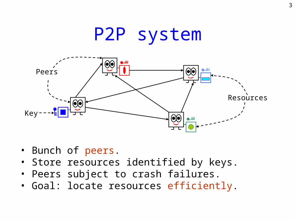
P2P system

• Bunch of peers. • Store resources identified by keys.• Peers subject to crash failures.• Goal: locate resources efficiently.

Resources

Peers

Key

4

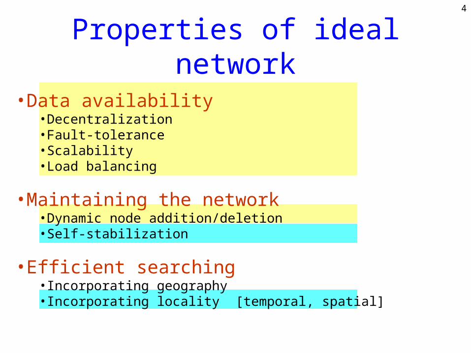
Properties of ideal network

•Data availability•Decentralization•Fault-tolerance•Scalability•Load balancing

•Maintaining the network•Dynamic node addition/deletion•Self-stabilization

•Efficient searching•Incorporating geography•Incorporating locality [temporal, spatial]

5

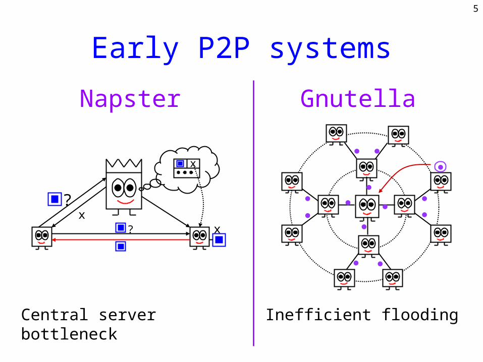
Early P2P systems

Napster

?

x

x? x

Central server bottleneck

Gnutella

Inefficient flooding

6

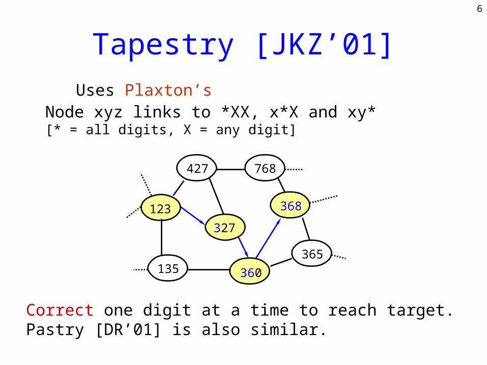
Tapestry [JKZ’01]Uses Plaxton’s Algorithm:

Correct one digit at a time to reach target. Pastry [DR’01] is also similar.

427

327

768

368

135 360

365

123

Node xyz links to *XX, x*X and xy* [* = all digits, X = any digit]

7

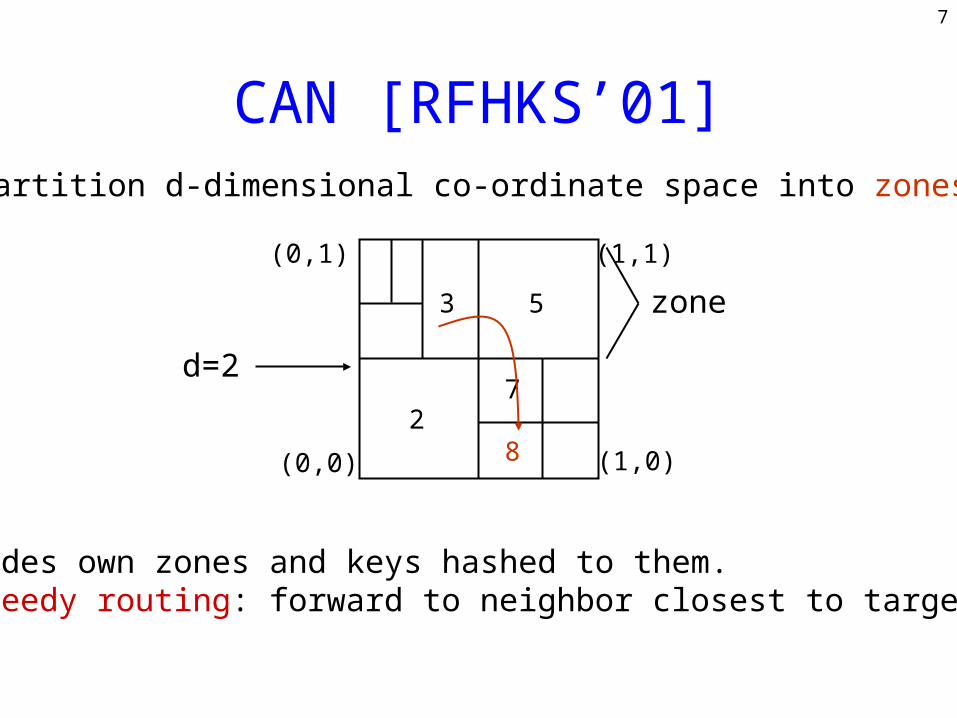
CAN [RFHKS’01]

3 5

7

82

(0,0) (1,0)

(0,1) (1,1)

Partition d-dimensional co-ordinate space into zones.

Nodes own zones and keys hashed to them.Greedy routing: forward to neighbor closest to target.

d=2

zone

8

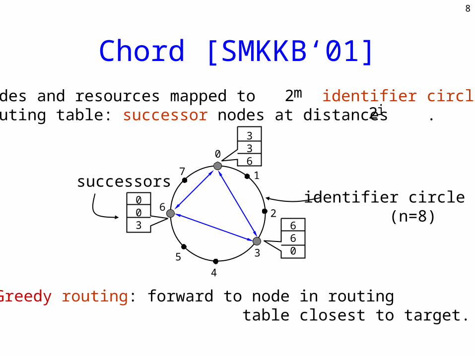
Chord [SMKKB‘01]Nodes and resources mapped to identifier circle.Routing table: successor nodes at distances .

0

1

2

3

4

7

6

5

Greedy routing: forward to node in routing table closest to target.

660

003

336

successorsidentifier circle (n=8)

m2i2

9

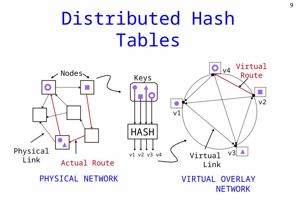
Distributed Hash Tables

v2

HASH

v1

v4

v3 v1 v2 v3 v4

KeysNodes

Actual Route

Physical Link

Virtual Link

Virtual Route

PHYSICAL NETWORK VIRTUAL OVERLAY NETWORK

10

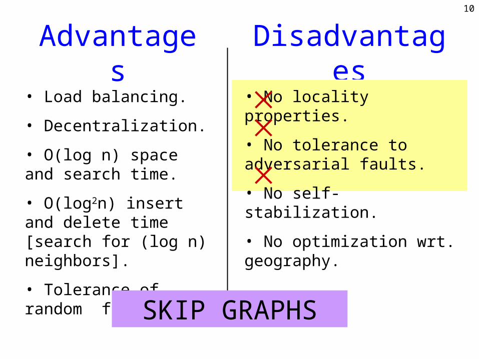
Advantages

Disadvantages

• Load balancing.

• Decentralization.

• O(log n) space and search time.

• O(log2n) insert and delete time [search for (log n) neighbors].

• Tolerance of random faults.

SKIP GRAPHS

• No locality properties.

• No tolerance to adversarial faults.

• No self-stabilization.

• No optimization wrt. geography.

11

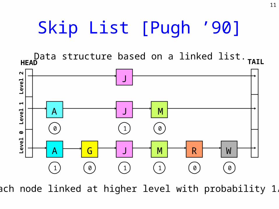
Skip List [Pugh ’90]

Data structure based on a linked list.

A G J M R W

HEAD TAIL

1 0 1 1 00

0 01

Each node linked at higher level with probability 1/2.

Level 0

A J M

Level 1

J

Level 2

12

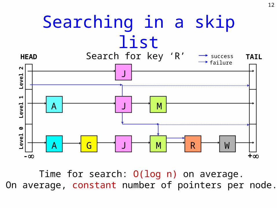
Searching in a skip list

A G J M R W

HEAD TAIL

A J

J

Search for key ‘R’

M

Time for search: O(log n) on average.On average, constant number of pointers per node.

Level 0

Level 1

Level 2

- +

successfailure

13

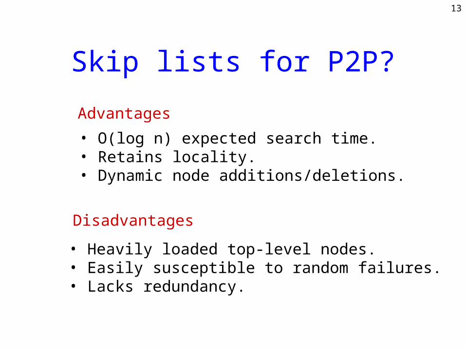
Skip lists for P2P?

• Heavily loaded top-level nodes.• Easily susceptible to random failures.• Lacks redundancy.

Disadvantages

Advantages

• O(log n) expected search time.• Retains locality.• Dynamic node additions/deletions.

14

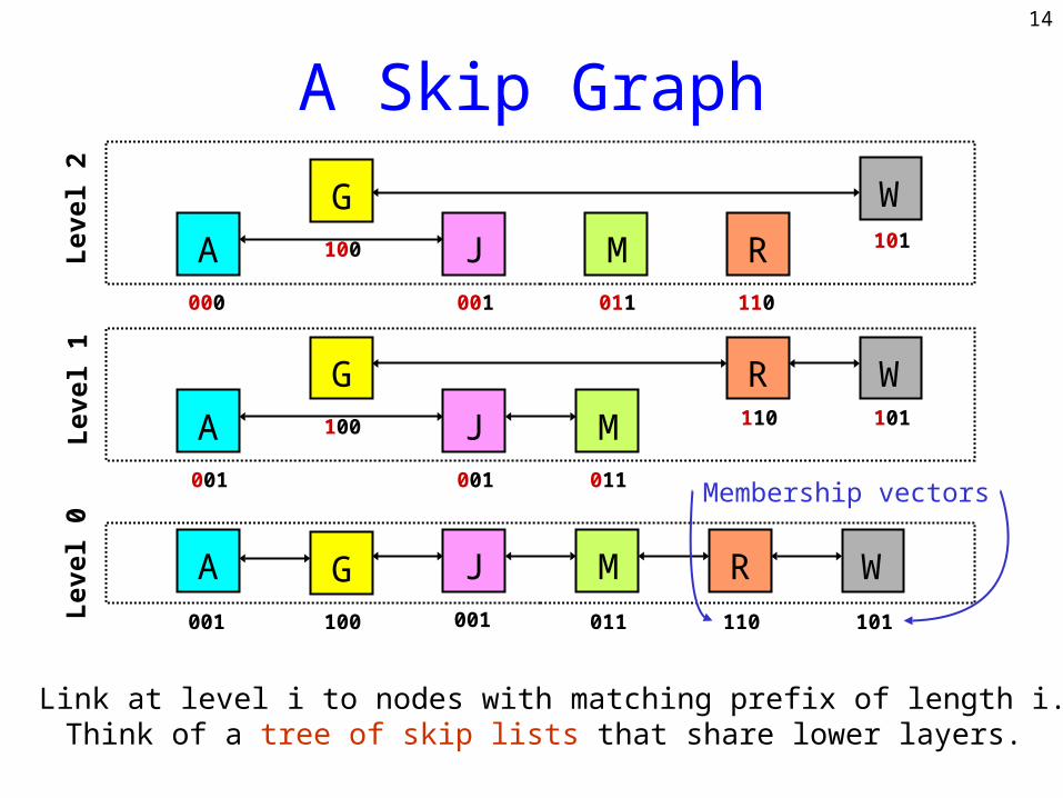
A Skip Graph

A001

J001

M011

G100

W101

R110

Level 1

G

R

W

A J M000 001 011

101

110

100Level 2

A G J M R W001 001 011100 110 101Level 0

Membership vectors

Link at level i to nodes with matching prefix of length i.Think of a tree of skip lists that share lower layers.

15

Properties of skip graphs

1. Searching.

2. Node insertions.

3. Independence from system size.

4. Locality and range queries.

16

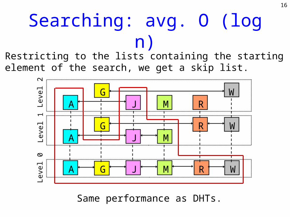
Searching: avg. O (log n)

Same performance as DHTs.

A J MG WR

Level 1

GR

WA J MLe

vel 2

A G J M R W

Level 0

Restricting to the lists containing the starting element of the search, we get a skip list.

17

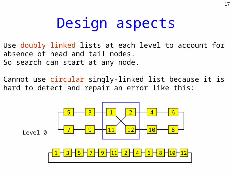
Use doubly linked lists at each level to account for absence of head and tail nodes.So search can start at any node.

Cannot use circular singly-linked list because it is hard to detect and repair an error like this:

5 3 1

7 9 11

2 4 6

12 10 8

51 3 117 9 62 4 128 10

Level 0

Design aspects

18

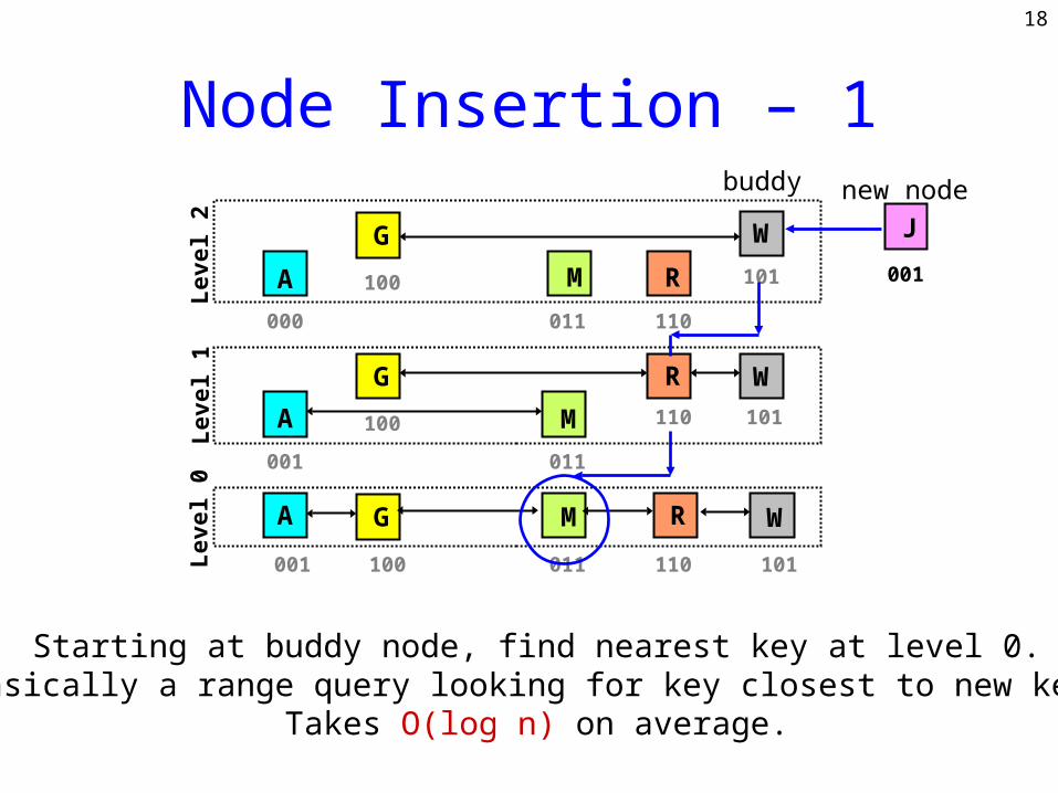
Node Insertion – 1

A

001

M

011

G

100

W

101

R

110

Level 1

G

R

W

A M

000 011

101

110

100Level 2

A G M R W

001 011100 110 101Level 0

J

001

Starting at buddy node, find nearest key at level 0.Basically a range query looking for key closest to new key.

Takes O(log n) on average.

buddy new node

19

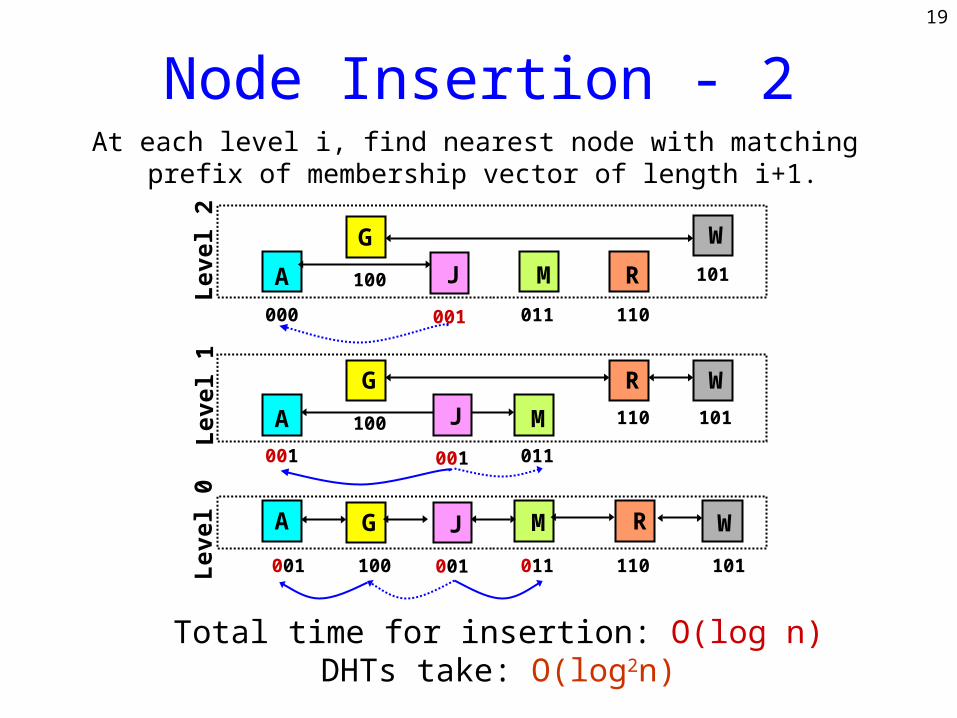
Node Insertion - 2At each level i, find nearest node with matching

prefix of membership vector of length i+1.

A

001

M

011

G

100

W

101

R

110

Level 1G

R

W

A M

000 011

101

110

100Level 2

A G M R W

001 011100 110 101Level 0

J

001

J

001

J

001

Total time for insertion: O(log n)DHTs take: O(log2n)

20

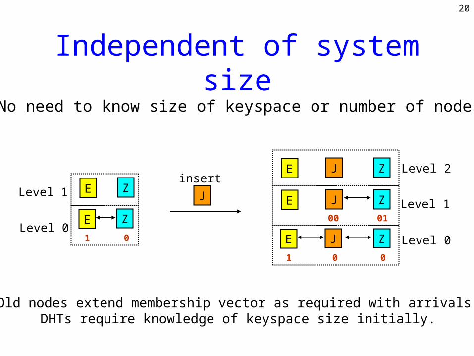
Independent of system size

No need to know size of keyspace or number of nodes.

E Z

1 0

E ZJ

insert

Level 0

Level 1

E Z

1 0

E Z

J

0

J00 01

E ZJ

Level 0

Level 1

Level 2

Old nodes extend membership vector as required with arrivals.DHTs require knowledge of keyspace size initially.

21

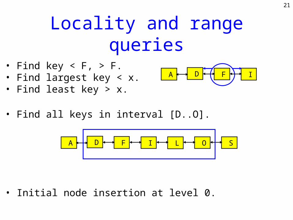
Locality and range queries

• Find key < F, > F.• Find largest key < x.• Find least key > x.

• Find all keys in interval [D..O].

• Initial node insertion at level 0.

D F A I

D F A I L O S

22

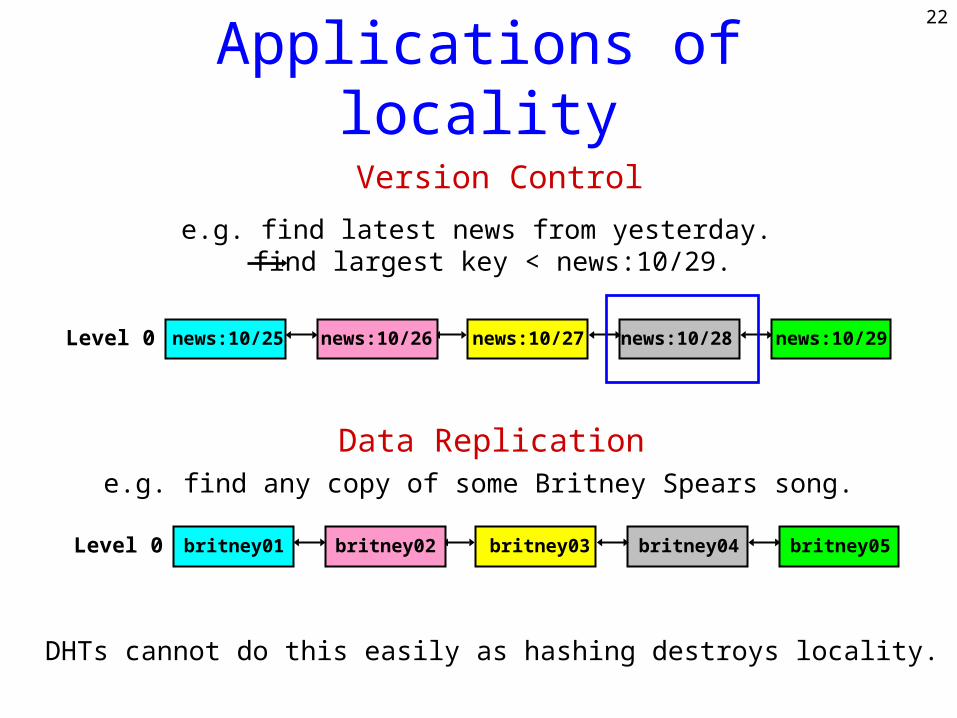
Applications of locality

news:10/29

e.g. find latest news from yesterday. find largest key < news:10/29.

news:10/27 news:10/28news:10/26news:10/25Level 0

DHTs cannot do this easily as hashing destroys locality.

e.g. find any copy of some Britney Spears song.

britney05britney03 britney04britney02britney01Level 0

Data Replication

Version Control

23

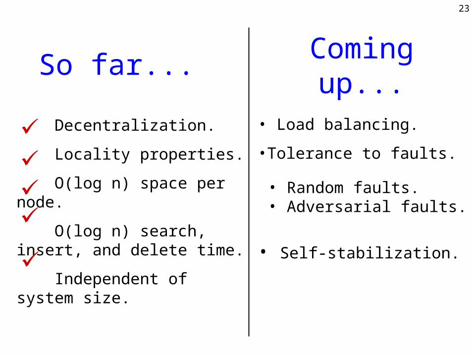
So far...

Decentralization.

Locality properties.

O(log n) space per node.

O(log n) search, insert, and delete time.

Independent of system size.

Coming up...

• Load balancing.

•Tolerance to faults.

• Self-stabilization.

• Random faults.• Adversarial faults.

24

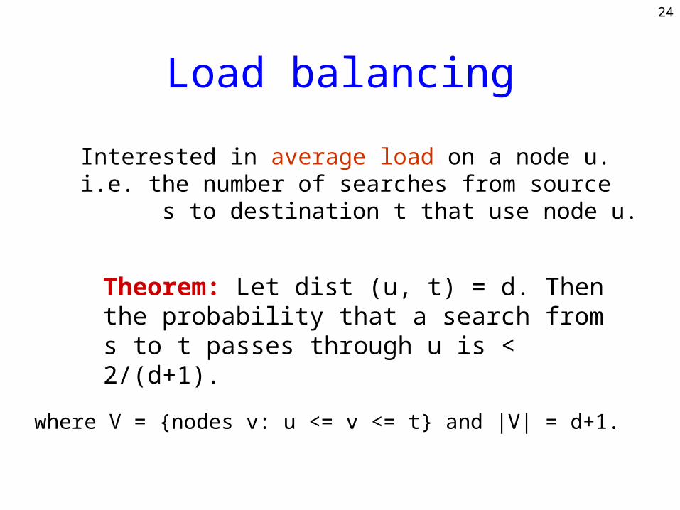
Load balancing

Interested in average load on a node u.i.e. the number of searches from source s to destination t that use node u.

Theorem: Let dist (u, t) = d. Then the probability that a search from s to t passes through u is < 2/(d+1).

where V = {nodes v: u <= v <= t} and |V| = d+1.

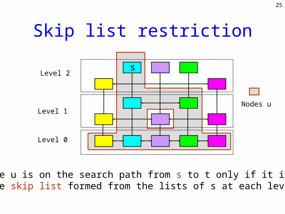
25

Nodes u

Skip list restriction

Level 0

Level 1

Level 2

Node u is on the search path from s to t only if it is inthe skip list formed from the lists of s at each level.

s

26

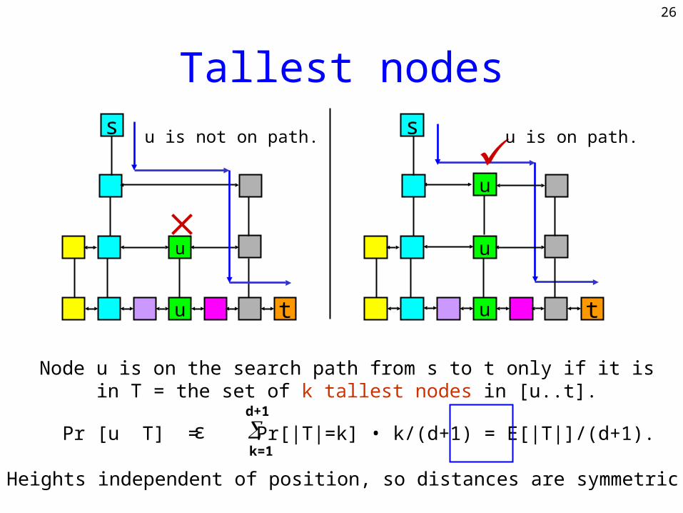
Tallest nodes

Node u is on the search path from s to t only if it isin T = the set of k tallest nodes in [u..t].

u

u t

s u is not on path.

tu

u

s

u

u is on path.

Pr [u T] = Pr[|T|=k] • k/(d+1) = E[|T|]/(d+1).ε k=1

d+1

Heights independent of position, so distances are symmetric.

27

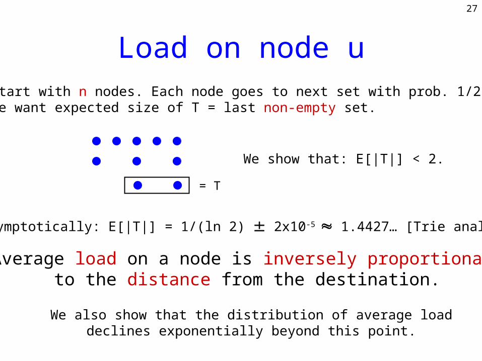
Load on node uStart with n nodes. Each node goes to next set with prob. 1/2.We want expected size of T = last non-empty set.

= T

Average load on a node is inversely proportional to the distance from the destination.

We show that: E[|T|] < 2.

Asymptotically: E[|T|] = 1/(ln 2) 2x10-5 1.4427… [Trie analysis]

We also show that the distribution of average loaddeclines exponentially beyond this point.

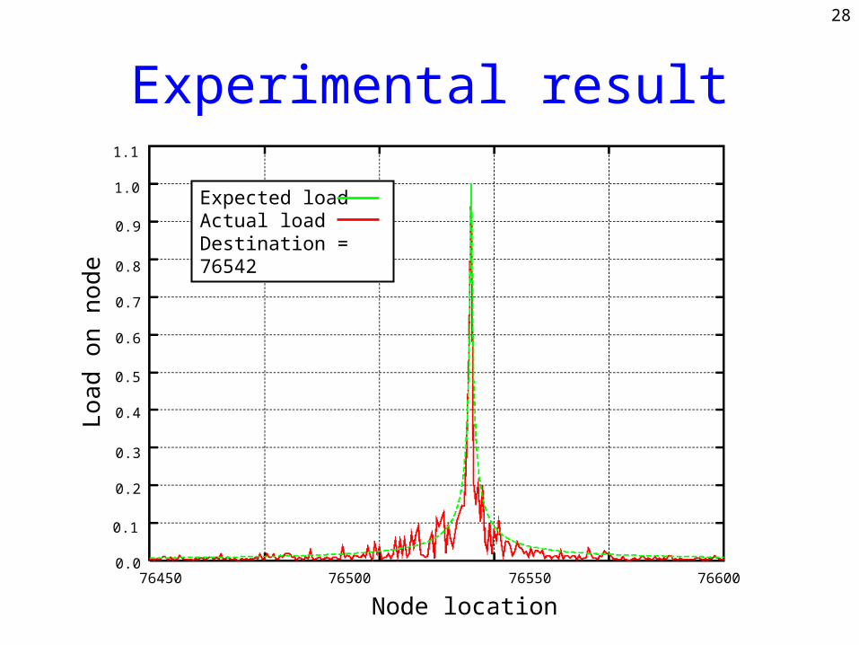
28

Expected loadActual loadDestination = 76542

76400 76450 76500 76550 76600 76650

0.1

0.2

0.3

0.4

0.5

0.6

0.7

0.8

0.9

1.0

1.1

0.0

Node location

Load

on

nod

eExperimental result

29

Fault tolerance

How do node failures affect skip graph performance?

Random failures: Randomly chosen nodes fail. Experimental results.

Adversarial failures: Adversary carefully chooses nodes that fail. Bound on expansion ratio.

30

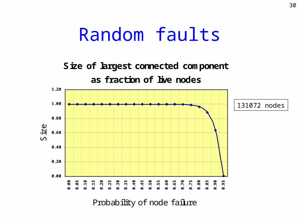
Random faults

Size of largest connected component

as fraction of live nodes

0.00

0.20

0.40

0.60

0.80

1.00

1.20

0.0

0

0.0

5

0.1

0

0.1

5

0.2

0

0.2

5

0.3

0

0.3

5

0.4

0

0.4

5

0.5

0

0.5

5

0.6

0

0.6

5

0.7

0

0.7

5

0.8

0

0.8

5

0.9

0

0.9

5

Probability of node failure

Siz

e

131072 nodes

31

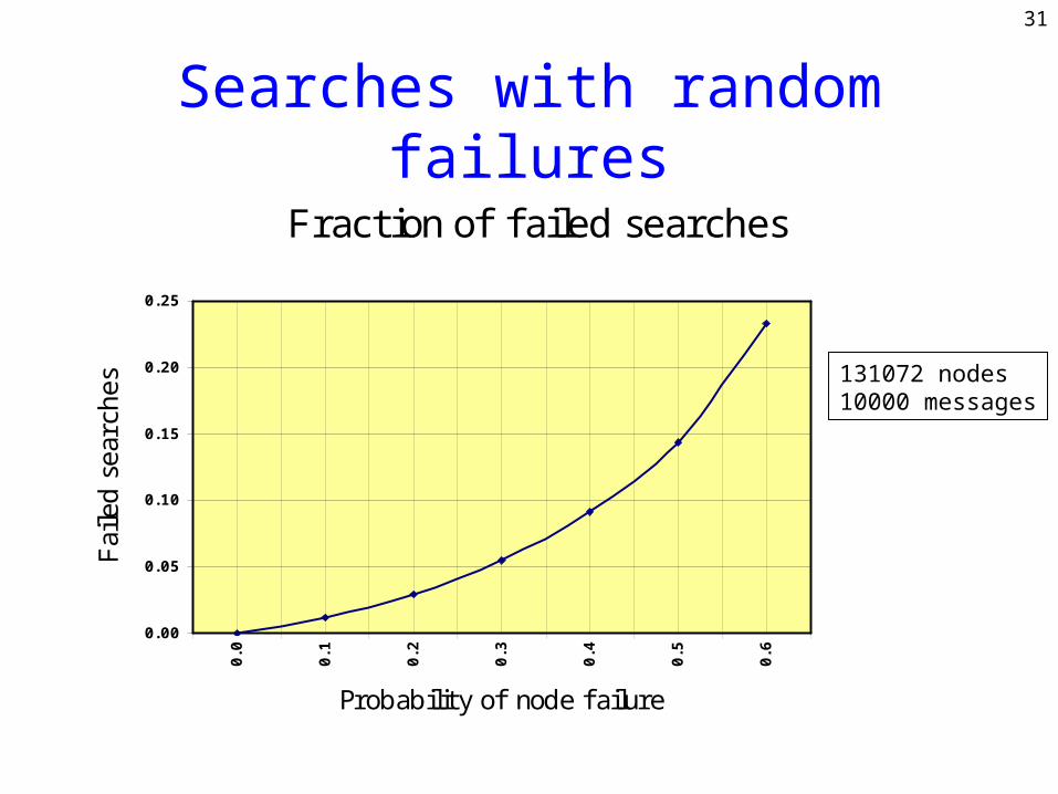
Searches with random failures

Fraction of f ailed searches

0.00

0.05

0.10

0.15

0.20

0.25

0.0

0.1

0.2

0.3

0.4

0.5

0.6

Probability of node f ailure

Fai

led s

earc

hes 131072 nodes

10000 messages

32

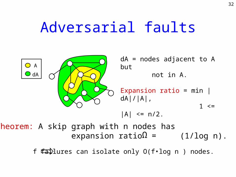
Adversarial faults

Theorem: A skip graph with n nodes has expansion ratio = (1/log n).Ω

A

dA

dA = nodes adjacent to A but not in A.

Expansion ratio = min |dA|/|A|, 1 <= |A| <= n/2.

f failures can isolate only O(f•log n ) nodes.

33

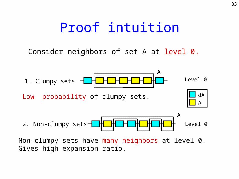
Proof intuition

Consider neighbors of set A at level 0.

A Level 01. Clumpy sets

A

2. Non-clumpy sets Level 0

Low probability of clumpy sets.

Non-clumpy sets have many neighbors at level 0.Gives high expansion ratio.

AdA

34

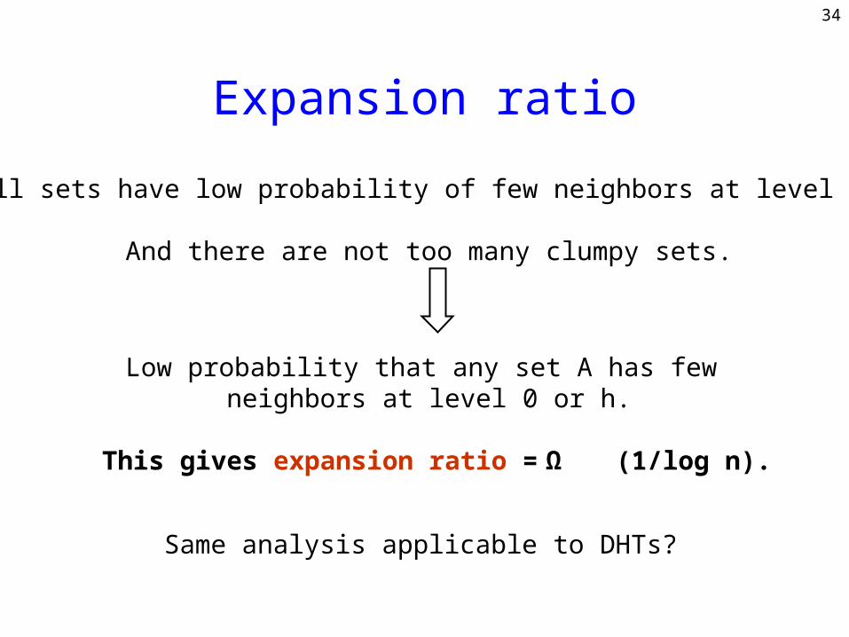
Expansion ratio

All sets have low probability of few neighbors at level h.

And there are not too many clumpy sets.

Low probability that any set A has few neighbors at level 0 or h.

This gives expansion ratio = (1/log n).Ω

Same analysis applicable to DHTs?

35

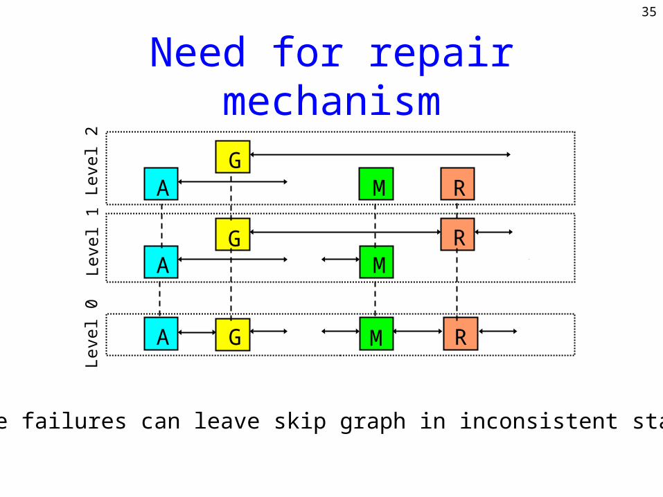
Need for repair mechanism

A J MG WR

Level 1

GR

WA J MLe

vel 2

A G J M R W

Level 0

Node failures can leave skip graph in inconsistent state.

36

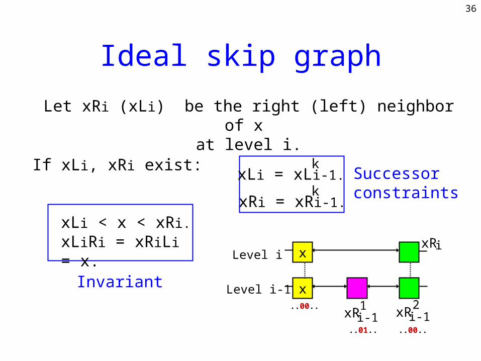
Ideal skip graph

Let xRi (xLi) be the right (left) neighbor of x at level i.

xLi < x < xRi.xLiRi = xRiLi = x.

Invariant

kxRi = xRi-1.

kxLi = xLi-1. Successor

constraints

x

Level i

Level i-1

ixR

i-1xR1

i-1xR2

x

..00..

..01.. ..00..

If xLi, xRi exist:

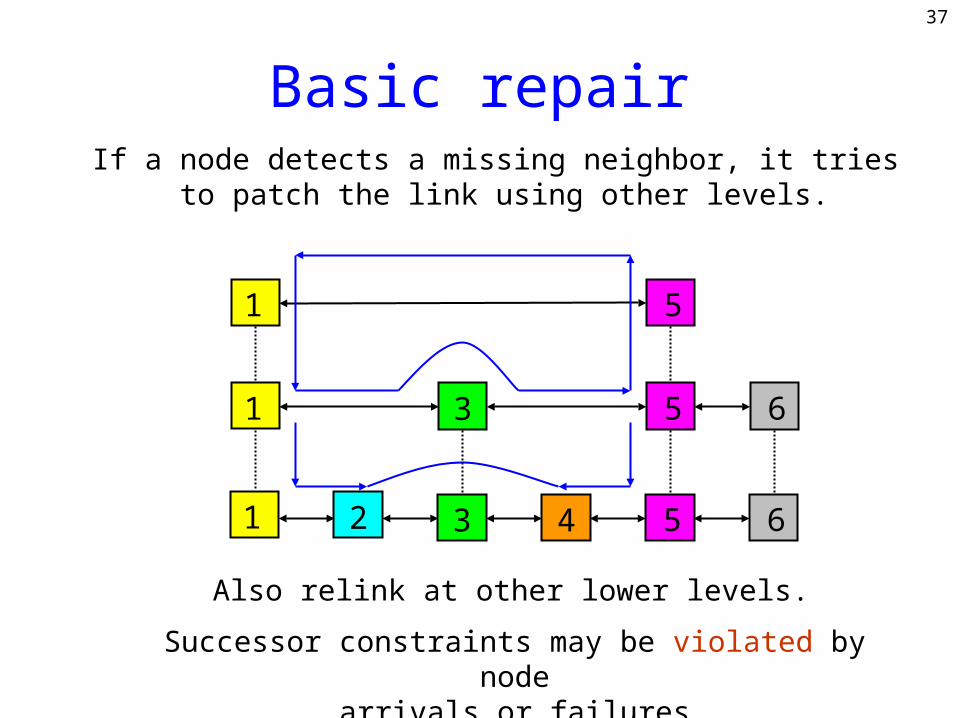
37

Basic repairIf a node detects a missing neighbor, it tries

to patch the link using other levels.

1 2 4 5 63

31 5 6

1 5

Also relink at other lower levels.

Successor constraints may be violated by node arrivals or failures.

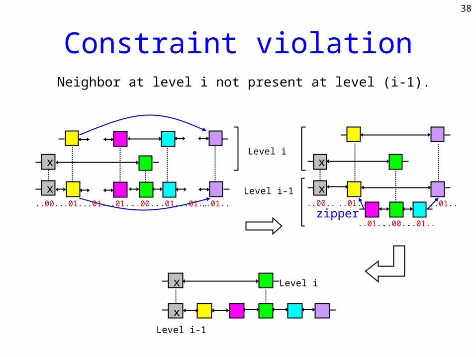
38

Constraint violationNeighbor at level i not present at level (i-1).

x

x Level i-1

Level i

Level i-1

Level ix

x

zipper..00.. ..01.. ..01.. ..01.. ..00.. ..01.. ..01....01.. ..00.. ..01..

..01.. ..00.. ..01..

x

x..01..

39

A C

B

D

E

F

G H I

JzipperOp message

Level i

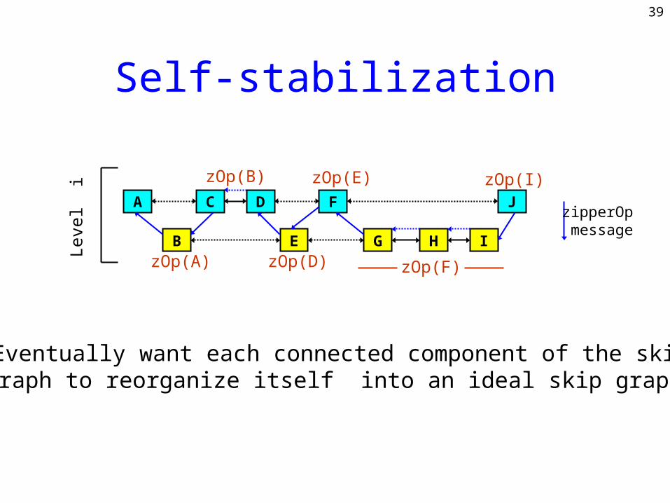
Self-stabilization

zOp(I)

zOp(F)

zOp(E)

zOp(D)

zOp(B)

zOp(A)

Eventually want each connected component of the skipgraph to reorganize itself into an ideal skip graph.

40

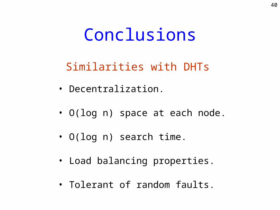
Conclusions

• Decentralization.

• O(log n) space at each node.

• O(log n) search time.

• Load balancing properties.

• Tolerant of random faults.

Similarities with DHTs

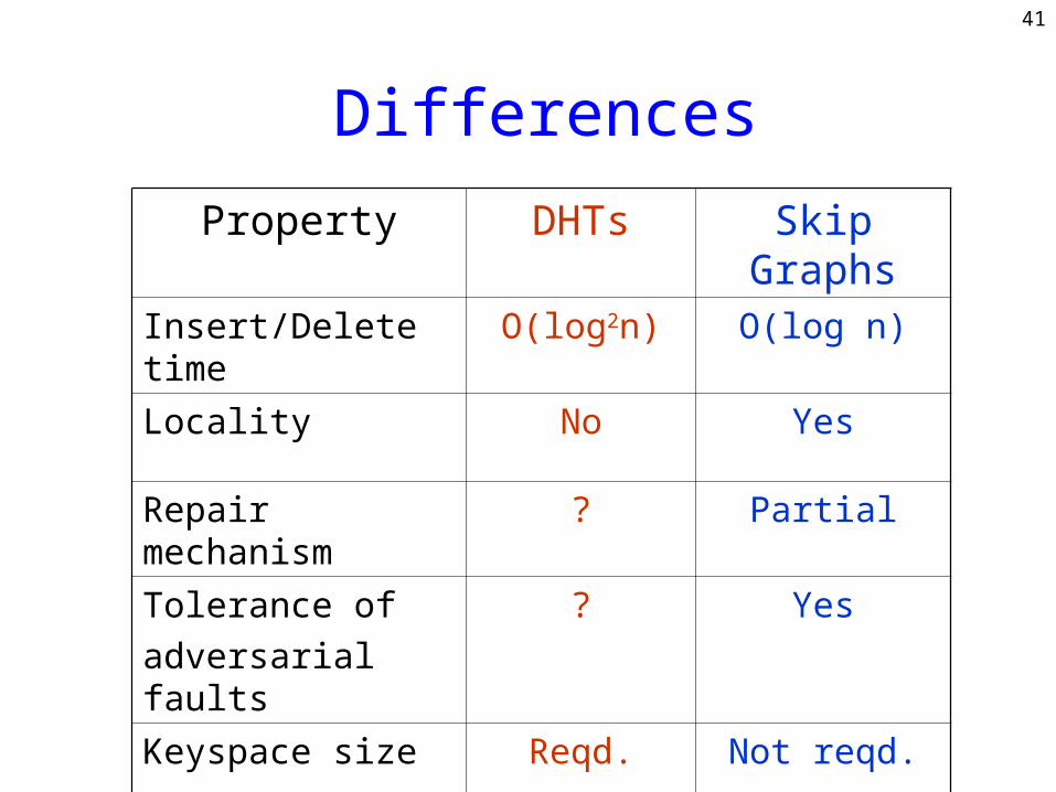
41

Property DHTs Skip Graphs

Insert/Delete time

O(log2n) O(log n)

Locality No Yes

Repair mechanism

? Partial

Tolerance ofadversarial faults

? Yes

Keyspace size Reqd. Not reqd.

Differences

42

Open Problems

• Evaluate performance in practice.

• Incorporate geographical proximity.

• Study multi-dimensional skip graphs.

• Study effect of byzantine failures.

?

• Design efficient repair mechanism.