SKIN CANCER MALIGNANCY CLASSIFICATION WITH TRANSFER LEARNING

by

Recep Erol

A thesis presented to the Department of Computer Science

and the Graduate School of University of Central Arkansas in partial

fulfillment of the requirements for the degree of

Master of Science

in

Applied Computing

Conway, Arkansas

August 2018

PERMISSION

Title Skin Cancer Malignancy Classification with Transfer Learning

Department Computer Science

Degree Master of Science

In presenting this thesis/dissertation in partial fulfillment of the requirements for a

graduate degree from the University of Central Arkansas, I agree that the Library of this

University shall make it freely available for inspections. I further agree that permission

for extensive copying for scholarly purposes may be granted by the professor who

supervised my thesis/dissertation work, or, in the professor’s absence, by the Chair of the

Department or the Dean of the Graduate School. It is understood that due recognition

shall be given to me and to the University of Central Arkansas in any scholarly use which

may be made of any material in my thesis/dissertation.

Recep Erol

July 18, 2018

iv

© 2018 Recep Erol

v

ACKNOWLEDGEMENTS

I would like to thank my supervisor Dr. Sinan Kockara, and my committee members,

Dr. Olcay Kursun and Dr. Mahmut Karakaya, for supporting and guiding me, sharing

their knowledge, and helping me learn and become a better researcher over the duration

of my master’s program.

Also, my appreciation and my sincere thanks go to my parents (Sevil (rest in peace)

and Hamza), in-laws (Fatma and Halit), and my sister (Ozge) for being all the way with

me.

Finally, special thanks are reserved for my wife, Humeyra. You have been

continually supportive of my graduate education. You have been patient with me when

I’m frustrated, you celebrated with me when even the littlest things go right, and you are

there whenever I need you to just listen.

vi

ABSTRACT

Malignant melanoma is the deadliest form of skin cancer. Dermoscopy is a

noninvasive high-resolution imaging technique that assists physicians for more accurate

diagnoses of skin cancers. Melanoma is a fast-growing aggressive type of skin cancer.

Due to this feature, malignant melanoma remains one of the fastest growing cancers

worldwide. After it metastasizes from its origin into other tissues, the response rate to

treatment declines as low as 5%, and its 10-year survival rate is only about 10%. After it

metastasizes, there is no surgical removal option available for treatment. Thus, early

detection of malignant melanoma is critically important. Among many types of skin

cancers, melanoma has the highest false negative ratio.

Therefore, this thesis proposes three methods for early detection of malignant

melanoma. More specifically, this thesis, first, introduces a novel approach of texture-

based abrupt cutoff quantification method (abrupt cutoff is one of the critical features for

detecting malignant melanoma in its early stages). In current clinical practice, abrupt

cutoff evaluation is subjective and error-prone. In our method, we introduce a novel

approach to objectively and quantitatively measure abrupt cutoff. To achieve this, we

quantitatively analyzed the texture features of a region within the skin lesion boundary

using level set propagation (LSP) method. Then, we built feature vectors of homogeneity,

standard deviation of pixel values, and mean of the pixel values of the region of interest

between the contracted border and the original border of a skin lesion. These vectors

were then classified using neural networks (NN) and support vector machines (SVM)

classifiers. Results obtained from these classifiers are also compared.

vii

Second, to accurately and real-time segment skin lesions in dermoscopic images, we

used superpixels approach. More specifically, simple linear iterative clustering (SLIC)

superpixel algorithm is used. SLIC adapts k-means clustering to generate superpixels.

After superpixels are created from dermoscopy images, in order to automatically merge

meaningful superpixels that fall inside the skin lesion boundary, we first found the mean

average value of each superpixel, and second, we calculated the median threshold values

for all superpixels. After the merge of superpixels, we were able to accurately segment

skin lesion borders. Our results showed that our method provides comparable

segmentation results for skin lesions to the physician drawn lesion borders.

Third, for accurate and fast classification of malignant melanoma on dermoscopy

images, we used Inception v3 image classification transfer learning algorithm. We used

pretrained version of Inception v3 on ImageNet dataset. We achieved the accuracy of

95% f-1 score for classifying the malignancy on 4,572 dermoscopy images.

Keywords: Deep Learning, Transfer Learning, Melanoma, Malignant Melanoma,

Dermoscopy, SLIC, Skin Cancer Classification, Abrupt Cutoff Quantification, Skin

Lesion Segmentation

viii

TABLE OF CONTENTS

ACKNOWLEDGEMENTS ----------------------------------------------------------------------- v

ABSTRACT --------------------------------------------------------------------------------------- vi

LIST OF TABLES -------------------------------------------------------------------------------- xi

LIST OF FIGURES ------------------------------------------------------------------------------ xii

LIST OF EQUATIONS -------------------------------------------------------------------------- iv

CHAPTER 1. INTRODUCTION ---------------------------------------------------------------- 1

1.1. Motivation ------------------------------------------------------------------------------------ 1

1.2. Structure of the thesis ---------------------------------------------------------------------- 2

CHAPTER 2. AN OVERVIEW OF SKIN CANCER, HUMAN SKIN AND

DIAGNOSIS METHODS ------------------------------------------------------------------------- 3

2.1. Skin Cancer ---------------------------------------------------------------------------------- 3

2.2. Layers of Human Skin --------------------------------------------------------------------- 3

2.3. Skin Cancer ---------------------------------------------------------------------------------- 5

2.3.1. Melanoma --------------------------------------------------------------------------------- 8

2.3.2. Basal-Cell Carcinoma ------------------------------------------------------------------- 9

2.3.3. Squamous-Cell Carcinoma ------------------------------------------------------------- 9

2.4. Skin Cancer Imaging Techniques ------------------------------------------------------ 10

2.5. Diagnosis Methods of Skin Cancer ---------------------------------------------------- 12

CHAPTER 3. RELATED WORKS AND CURRENT TECHNOLOGY ----------------- 16

ix

3.1. Overview of Machine Learning ------------------------------------------------------------ 16

3.1.1. Categories of Machine Learning Algorithms--------------------------------------- 16

3.2. Neural Networks ------------------------------------------------------------------------------ 17

3.2.1. Convolutional Neural Networks ------------------------------------------------------ 18

3.3. Deep Learning and Transfer Learning ---------------------------------------------------- 20

CHAPTER 4. TEXTURE BASED SKIN LESION ABRUPTNESS QUANTIFICATION

TO DETECT MALIGNANCY ----------------------------------------------------------------- 22

4.1. Abrupt Cutoff Measurement from Dermoscopic Images -------------------------- 22

4.1.1. Boundary detection and boundary contour extraction -------------------------- 25

4.1.2. LSP for lesion border contraction --------------------------------------------------- 26

4.1.3. Eulerian Formulation ------------------------------------------------------------------ 31

4.1.4. Feature Extraction --------------------------------------------------------------------- 33

4.2. Data Analysis and Results --------------------------------------------------------------- 34

CHAPTER 5. SKIN CANCER MALIGNANCY CLASSIFICATION WITH

TRANSFER LEARNING ----------------------------------------------------------------------- 42

5.1. Introduction -------------------------------------------------------------------------------- 42

5.2. Dermoscopy Image Preprocessing ----------------------------------------------------- 44

5.2.1. Image Segmentation ------------------------------------------------------------------- 44

5.2.2. Cropping and Image Resampling --------------------------------------------------- 46

5.2.3. Image Resizing with Adding Zero-Padding -------------------------------------- 47

5.3. Classification ------------------------------------------------------------------------------ 48

x

5.4. Experiments and Performance Analysis ---------------------------------------------- 49

5.5. Discussion ---------------------------------------------------------------------------------- 58

CHAPTER 6. CONCLUSIONS ---------------------------------------------------------------- 59

6.1. Skin Lesion Abruptness Quantification --------------------------------------------------- 59

6.2. Skin Lesion Classification using Transfer Learning------------------------------------ 60

REFERENCES ----------------------------------------------------------------------------------- 61

xi

LIST OF TABLES

Table 1: ABCD-E rule criteria for calculation of total dermoscopy score (TDS) [35]. .... 13 Table 2: Total dermoscopy score and its interpretation [35]. .......................................... 14 Table 3: LSP vs. DS based texture homogeneity feature extraction and classification of lesions with various classifiers: multi-layer perceptron, fully connected multi-hidden layer NN, and SVM. 10-fold cross-validation is used. Results listed here are means of 10 random executions. ........................................................................................................ 39 Table 4: The parameters of the NN (the multi-layer perceptron and the fully-connected multi-hidden layer NN) classifiers and SVM. ................................................................ 40 Table 5: Results of experiment 1 with 13684 images. .................................................... 50 Table 6: Results of experiment 2 with 1,984 images using transfer learning. .................. 51 Table 7: Results of experiment 3 with 13,684 images using transfer learning. ................ 52 Table 8: Results of the experiment 4. ............................................................................. 56

xii

LIST OF FIGURES Figure 1: The epidermis and dermis layers in human skin with squamous cells, basal cells and melanocyte [18]. ....................................................................................................... 5 Figure 2: A red patch (a) and open sore (b) types of basal-cell carcinoma [44]. ............... 9 Figure 3: An elevated growth (a) and irregular borders (b) of squamous-cell carcinoma [46]. .............................................................................................................................. 10 Figure 4: (a) is the perceptron layer and (b) is the image of Multi-layer Neural Network. ...................................................................................................................................... 17 Figure 5: An example of a convolutional neural network [57]. ....................................... 19 Figure 6: Global workflow is shown. ............................................................................. 23 Figure 7: (a) represent a malignant case with abrupt cutoff where the lesion is divided into eight pieces and asterisks indicate abrupt cut off (b) represents a benign case with gradual change at lesion border. In both cases, homogeneity feature is a strong indicator for evaluating the abruptness. ........................................................................................ 24 Figure 8: Chain code initialization is shown. ................................................................. 25 Figure 9: The starting point is shown in (a), and the lesion boundary is represented in green in (b). ................................................................................................................... 26 Figure 10: In (a) and (b), red curves represent the contracted border. (a) The curve set shows that the LSP can obtain quantitatively accurate results. (b) The curve set shows the DS still suffers from high curvatures and cannot offer constant distance from the original curve. (c) shows that the DS yields a deficient data collection along the layer where the abruptness is searched. Yellow brushes indicate that not equal amount of territory considered for feature extraction in spanning windows. Note that, these regions are masked using polygon intersection operations prior to feature extraction. (d) shows that the constant velocity LSP imbues equalization of data amount during feature extraction. ...................................................................................................................................... 27 Figure 11: (a) Without entropy condition stability can be preserved if contraction distance is less than the curvature of an arbitrary 2d curve; (b) Cusps emerge when contraction distance is greater than the curvature. Shocks and cusps can be avoided adopting entropy condition. ...................................................................................................................... 30 Figure 12: Homogeneity extraction from the highlighted region along the lesion boundary. ...................................................................................................................... 34 Figure 13: Multi-layer Perception with a single hidden layer NN architecture. ............... 37

xiii

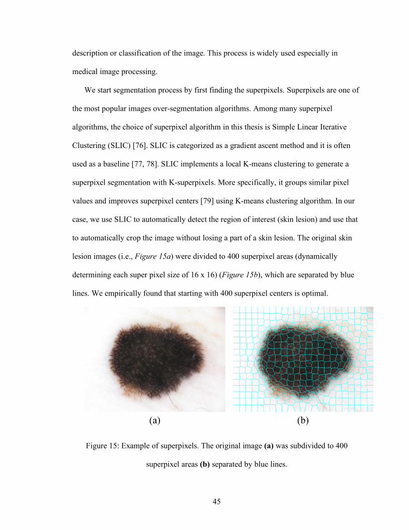
Figure 14: Fully-connected multi-hidden layer NN architecture. .................................... 38 Figure 15: Example of superpixels. The original image (a) was subdivided to 400 superpixel areas (b) separated by blue lines. .................................................................. 45 Figure 16: Images after each preprocessing steps: (a) is the original image obtained from ISIC 2018 Challenge, (b) is the segmentation mask of the image, (c) is the overlap of (a) and (b), (d) is framing the Region of Interest, and (e) is the cropped and resized to n x n image. ........................................................................................................................... 47 Figure 17: Google Inception v3 transfer learning algorithm layers [86]. ......................... 48 Figure 18: (a) is the original image, (b) is the segmentation mask drawn by a physician, (c) segmentation mask that is the result of our segmentation algorithm. ......................... 54 Figure 19: Square malignant image after resizing process. ............................................. 55 Figure 20: Accuracies of training and validation for each iteration. ................................ 57 Figure 21: Cross-entropies of training and validation. .................................................... 57

iv

LIST OF EQUATIONS

Equation 1 ..................................................................................................................... 13 Equation 2 ..................................................................................................................... 18 Equation 3 ..................................................................................................................... 28 Equation 4 ..................................................................................................................... 28 Equation 5 ..................................................................................................................... 28 Equation 6 ..................................................................................................................... 28 Equation 7 ..................................................................................................................... 29 Equation 8 ..................................................................................................................... 31 Equation 9 ..................................................................................................................... 31 Equation 10 ................................................................................................................... 32 Equation 11 ................................................................................................................... 32 Equation 12 ................................................................................................................... 32 Equation 13 ................................................................................................................... 32 Equation 14 ................................................................................................................... 32 Equation 15 ................................................................................................................... 33 Equation 16 ................................................................................................................... 34

1

CHAPTER 1. INTRODUCTION

1.1. Motivation

The occurrence of malignant melanoma, which is the deadliest form of skin cancers,

has been elevated in the last decade. Between 2009 and 2010, the mortality rate due to

melanoma increased by 3% in the USA [1]. Skin cancer occurrence has become more

common not only in the USA but also in different countries with Caucasian people

majority such as the UK and Canada with 10,000 diagnoses and annual mortality of 1,250

people [2]. Early diagnosis of the melanoma has been spotlighted due to the persistent

elevation of the number of incidents, the high medical cost, and increased death rate. The

developments in computer-aided diagnostic methods can have a vital role on significantly

reducing mortality.

Dermoscopy, which is one of the noninvasive skin imaging techniques, has become a

key method in the diagnosis of melanoma. Dermoscopy is the method that magnifies the

region of interest (ROI) optically and takes digital pictures of the ROI. Misdiagnosis or

underdiagnosis of melanoma is the main reason for skin cancer-related fatalities [3]. The

cause of these errors is usually due to the complexity of the subsurface structures and the

subjectivity of visual interpretations [4, 5]. Hence, there is a need for computerized image

understanding tools to help physicians or primary care assistants to minimize the

diagnostic errors.

Expert clinicians look for the presence of exclusive visual features to diagnose skin

lesions correctly in almost all of the clinical dermoscopy methods. These features are

evaluated for irregularities and malignancy [6, 7, 8, 9]. However, in the case of an

inexperienced dermatologist, diagnosis of melanoma can be very challenging. The

2

accuracy of melanoma detection with dermoscopy still varies from 75-85% [10]. This

indicates the necessity of computer aided diagnosis platforms.

The problems addressed in this thesis are; i) how to eliminate the subjectivity on

visual interpretation of dermoscopy images for border irregularity/abruptness; ii) how to

improve the performance of feature extraction algorithms by providing more accurate

skin lesion segmentations; and iii) how to reduce the number of false-negative diagnosis.

Images used in this thesis are obtained from the International Skin Imaging

Collaborations Archive [11].

1.2. Structure of the thesis

The rest of the thesis is organized as follows:

Chapter 2 provides some fundamental and necessary background on human skin and

skin cancer types and our motivation to tackle this problem from a computer science

perspective.

Chapter 3 gives a brief introduction to deep learning, convolutional neural networks,

and finally transfer learning for their applications in various medical image processing

application areas, specifically for skin cancer field.

Chapter 4 describes our approach to skin lesion abruptness quantification that we

developed to objectively measure skin lesion borders’ abrupt cutoff.

Chapter 5 describes our approach for accurately segmenting skin lesions from

dermoscopy images and our solution to classify malignancy in dermoscopy images using

the transfer learning algorithm, Inception v3 [12] .

Chapter 6 concludes the thesis and summarizes our contributions.

3

CHAPTER 2. AN OVERVIEW OF SKIN CANCER, HUMAN SKIN AND DIAGNOSIS METHODS

2.1. Skin Cancer

Cancer is one of the leading causes of death of human beings. According to the World

Health Organization statistics, it is predicted that cancer will be the biggest cause of death

(13.1 million) by 2030 [13, 14]. Among all cancer types, skin cancer is the most common

form of cancer in the USA [4]. Based on the predictions, 20% of Americans will develop

skin cancer during their lifetime [7].

Skin cancer is not necessarily fatal. However, diagnosis in early stages plays a vital

role on saving lives. In order to understand the early detection and diagnosis of skin

cancer, it is important to examine human skin and different types of skin cancers.

Hereunder, this chapter is divided into three parts; the first part describes the layers of

human skin, the second part explains the different types of skin cancers, and the third part

focuses on computer-aided diagnosing techniques in details.

2.2. Layers of Human Skin

Skin is the largest organ in the human body with an average surface area of 1.5-2.0

square meters. It keeps the body safe from ultraviolet radiation (UV) and pathogens [15],

regulates body temperature, controls evaporation [16], and synthesizes vitamin D. Skin is

comprised of three main layers: the epidermis, the dermis, and the hypodermis.

§ Epidermis: The epidermis is the top layer of human skin that is built of multi-

layered squamous cells along with basal lamina. Squamous cells are flat cells of

the skin where basal cells are round cells below the squamous cells.

4

The epidermis does not contain any blood vessel, and oxygen reaches to the cells

in the deepest layer through diffusion [17]. Skin color is determined by the

melanin pigment which is found in the deepest layer of the epidermis.

§ Dermis: This layer is the second layer underneath the epidermis. It consists of

different cell types that build sweat glands and blood vessels. The dermis protects

the body from stress and strain by working like a cushion.

§ Hypodermis: Even though the hypodermis is listed as a part of the skin, it is not

always considered as a layer of the skin. It is found below the dermis and

connects the skin to the bone and muscles. The hypodermis contains connective

and fat (adipose) tissue. Figure 1 shows the layers and building block of cells of

these layers.

5

Figure 1: The epidermis and dermis layers in human skin with squamous cells, basal cells and melanocyte [18] (For the National Cancer Institute © (2008) Terese Winslow LLC,

U.S. Govt. has certain rights). 2.3. Skin Cancer

The human body is made of living cells which grow, divide into new cells, and die.

Cell division is a continuous process in the human body and is a replacement of dying

cells. However, growing of abnormal cells and uncontrollable cell division are the causes

of cancer [19].

Skin cancer is one of the most common cancers in human beings, and it arises from

the skin due to the abnormal growth of the cells that can easily invade and spread to the

other parts of the human body [20] . There are three main categories of skin cancers: (1)

Malignant melanoma, (2) Basal-cell carcinoma (BCC), (3) Squamous-cell carcinoma

(SCC). The BCC and SCC are types of non-melanoma skin cancers (NMSC).

6

Dermoscopy, a minimal invasive skin imaging technique, is one of the viable

methods for detecting melanoma and other pigmented skin proliferations. In the current

clinical settings, the first step of dermoscopic evaluation is to decide whether the lesion is

melanocytic or not. The second step is to find out whether the lesion is benign or

malignant. There are commonly accepted protocols to detect malignancy in skin lesions,

which are ABCD Rule, 7-point Checklist, Pattern Analysis, Menzies Method, Revised

Pattern Analysis, 3-point Checklist, 4-point Checklist, and CASH Algorithm [21, 22].

Celebi et al. [23] extracted shape, color, and texture features and fed these feature

vectors to a classifier such that they were ranked using feature selection algorithms to

determine the optimal subset size. Their approach yielded a specificity of 92.34% and a

sensitivity of 93.33% using 564 images. In their seminal work, Dreiseitl et al. [24]

analyzed the robustness of artificial neural networks (ANN), logistic regression, k-nearest

neighbors, decision trees, and support vector machines (SVMs) on classifying common

nevi, dysplastic nevi, and melanoma. They addressed three classification problems:

dichotomous problem of separating common nevi from melanoma and dysplastic nevi,

and the trichotomous problem of genuinely separating all these classes. They reported

that on both cases (dichotomous and trichotomous) logistic regression, ANNs and SVMs

showed the same performance, whereas k-nearest neighbor and decision trees performed

worse.

Rubegni et al. [25] extracted texture features, besides color and shape features. Their

ANN based approach reached the sensitivity of 96% and specificity 93% on a data set of

558 images containing 217 melanoma cases. Iyatomi et al. [26] proposed an internet-

based system which employs a feature vector consisting of shape, texture, and color

7

features. They achieved specificity and sensitivity of 86% using 1200 dermoscopy

images. Local methods have also been recently applied for skin lesion classification. Situ

et al. [27] offered a patch-based algorithm which used a Bag-of-Features approach. They

sampled the region of lesion into a 16 × 16 grid and extracted Wavelets and Gabor filters

as collecting 23 features in total. They compared two different classifiers which were

Naïve Bayes and SVM; the best performance they achieved was 82% specificity on a

dataset consisting of 100 images with 30 melanoma cases.

A considerable number of systems have been proposed for melanoma detection in the

last decade. Some of them aim to mimic the procedure that dermatologists pursue for

detecting and extracting dermoscopic features, such as granularities [28], irregular streaks

[29], regression structure [29], blotches [30], and blue-white veils [31]. These structures

are also used by dermatologists to score the lesion based on a seven point-checklist. Leo

et al. [32] described a CAD system that mimics the 7-point-checklist procedure.

However, approaches [23, 25, 33, 34] in the literature dominantly pursued pattern

recognition in melanoma detection. The majority of these works are inspired by the the

ABCD rule [35], and they extract the features according to the score table of ABCD

protocol. Shape features (e.g., irregularity, aspect ratio and maximum diameter,

compactness), which refer to both asymmetry and border, color features in several color

channels, and texture features (e.g., gray level co-occurrence matrix) [23] are the most

common features analyzed when the ABCD protocol is used [35]. There are other

approaches [33, 36, 37] that used one type of feature for detection of melanoma.

Seidenari et al. [33] aimed to distinguish atypical nevi and benign nevi using color

statistics in the RGB channel, such as mean, variance, and maximum RGB distance.

8

Their approach reached 86% accuracy, additionally they concluded that there was a

remarkable difference in distribution of pigments between the populations they studied.

Color histograms have been utilized for discriminating melanomas and atypical or benign

nevi [36, 37] with specificity little higher than 80%.

2.3.1. Melanoma

Melanoma is one of the deadliest and fastest growing cancer types in the world. In the

USA annually 3.5 million skin cancers are diagnosed. Skin cancer is rarely fatal except

melanoma which is the 6th common cancer type in the USA [38]. Women 25–29 years of

age are the most commonly affected group from melanoma. Ultraviolet tanning devices

are listed as known and probable human carcinogens along with plutonium and cigarettes

by the World Health Organization [38]. In 2017, an estimated 87,110 adults were

diagnosed with melanoma in the USA, and approximately 9,730 were fatal [39]. The

primary cause of melanoma is DNA damage due to the UV light exposure (i.e., sun light

and tanning beds). Genetics with history of malignant melanoma and having a fair skin

type are the other risk factors [40, 41].

Melanoma is a malignancy of melanocytes. Melanocytes are special cells in the skin

located in its outer epidermis. Since melanoma develops in the epidermis, it can be seen

by the human eye. Early diagnosis and treatment are critical to prevent harm. When

caught early, melanoma can be cured through excision operation. However, the high rate

of false-negative of malignant melanoma is the main challenge for early treatments [21].

Melanoma is commonly found on the lower limbs in female patients and on the back

in male patients [42], but it can also be found on other organs containing cells such as the

mouth and eye which is very rare [43].

9

2.3.2. Basal-Cell Carcinoma

The basal-cell carcinoma (BCC) is the most common form of skin cancer with at least

4 million cases in the U.S. annually. It arises from the deepest layer of the epidermis.

BCCs usually look like red patches or open sores (see Figure 2). There are very rare

cases of spreading of BCCs as they almost never spread [44], but people who have had

BCCs are prone to develop it again in their lifetime.

Figure 2: A red patch (a) and open sore (b) types of basal-cell carcinoma [44] (Figures

are reprinted with permission of Skin Cancer Foundation).

2.3.3. Squamous-Cell Carcinoma

Squamous-cell carcinoma (SCC) usually begins as a small lump, expands over time,

and turns into an ulcer. Compared to BCCs, SCCs have more irregular shapes with

crusted surface (Figure 3), and they are more likely to spread to the other organs [45].

Immunosuppression is another important risk factor of SCC along with UV exposure.

10

Figure 3: An elevated growth (a) and irregular borders (b) of squamous-cell carcinoma

[46] (Figures are reprinted with permission of Skin Cancer Foundation).

2.4. Skin Cancer Imaging Techniques

If it is diagnosed in early stages, skin cancer is 90% treatable compared to 50% in late

stages [47]. With the development of noninvasive and high-resolution imaging

techniques, the accuracy of in-situ diagnosis of skin cancers or skin lesions has increased

[48]. Especially, the lower diagnostic accuracy for melanoma is the major reason for over

treatment (caused by false positive diagnosis) or under treatment (caused by false

negative diagnosis). False positive diagnosis is the major contributor of excessive

treatment cost increases due to leading to excise an unnecessarily high number of benign

lesions for biopsy and pathological examination. However, high-resolution imaging

techniques have great potential to improve diagnostic specificity, and thus, these

techniques introduce a possibility of inducing a reduction in unnecessary excisions and

related costs. The most common imaging techniques currently used for diagnosis of skin

cancers are reflectance confocal microscopy, optical coherence tomography, ultrasound,

and dermoscopy.

11

§ Reflectance confocal microscopy (RCM)

Confocal microscopy is a noninvasive imaging method that uses a laser focused on a

specific point on the skin and visualizes the cellular details of the skin in-vivo. Because

cellular structures (cells, melanin, hemoglobin, etc.) have different refraction indexes,

RCM can easily differentiate reflected light from the skin. However, RCM is the costliest

among other skin imaging techniques.

§ Optical Coherence Tomography (OCT)

OCT can be used to image microscopic structures (few µm) in-vivo and can

distinguish healthy tissue from cancerous tissue. However, the OCT is not able to

visualize the subcellular elements and the membrane: it cannot detect the tumor in early

stages. Additionally, without histological confirmation, the OCT cannot fully determine

the diagnosis of melanoma. Thus, the OCT is not an advantageous way of melanoma

diagnosis process.

§ Ultrasound

Ultrasound is one of the most common noninvasive procedures as it is versatile, pain-

free, and has low risk. In this procedure, the skin morphology can be visualized by the

ultrasound waves that return from the tissue. Even though ultrasound waves can reach to

the deep skin layers and evaluate the tumor, the low resolution does not allow to

distinguish skin lesions histomorphologically. Also, it does not catch tumors at early

stages.

§ Dermoscopy

Dermoscopy, also known as epilumence microscopy (EM), is a noninvasive and in-

live method that is very practical for early detection of malignant melanoma and other

12

pigmented lesions. It allows users to capture the colors and subsurface structures of the

skin to detect melanoma in early stages. According to the statistics of the literature, using

dermoscopy can increase the accuracy of diagnosis between 5% and 30% depending on

the type of skin lesion [49, 50].

2.5. Diagnosis Methods of Skin Cancer

Visualizing skin lesions by any abovementioned imaging technique is not enough to

distinguish malignant melanoma from benign melanoma. There is a need for reproducible

diagnosis techniques that can be used by clinicians to understand the skin cancer types.

There are four commonly accepted reproducible methods for the diagnosis of skin

cancers especially melanoma. These are: i) ABCD-E rule, ii) the 3-point checklist, iii) the

7-point checklist, iv) the Menzies’ method, and v) pattern analysis.

§ ABCD-E Rule: This method was introduced in 1994 by Stolz et. al [35]. ABCD-

E stands for asymmetry, border, color, diameter, and evolving by time which are

five dermoscopic criteria for semi-quantitative assessment of skin lesions.

Melanomas are typically asymmetric with jagged edges and bigger than 6 mm.

They usually have mixed colors along with changing size, color, shape, and

bleeding. These criteria (except E) have their possible scores based on the look of

the skin lesion (Table 1). These scores are multiplied by associated weight factors

to yield a total dermoscopy score (TDS).

13

Table 1: ABCD-E rule criteria for calculation of total dermoscopy score (TDS) [35].

Criteria Possible Score Description Weight factor

Asymmetry 0-2 Assess contour, color and

structures

1.3

Border 0-8 Abrupt ending of pigment

pattern

0.1

Color 1-6 Presence of max 6 colors

(white, red, light brown, dark

brown, blue-gray, black)

0.5

Dermoscopic

Structures

1-5 Presence of network,

structureless areas, streaks, dots

and globules

0.5

TDS can be found using the equation below.

Equation 1

[(𝐴𝑠𝑐𝑜𝑟𝑒𝑥1.3) + (𝐵𝑠𝑐𝑜𝑟𝑒𝑥0.1) + (𝐶𝑠𝑐𝑜𝑟𝑒𝑥0.5) + (𝐷𝑠𝑐𝑜𝑟𝑒𝑥0.5)]

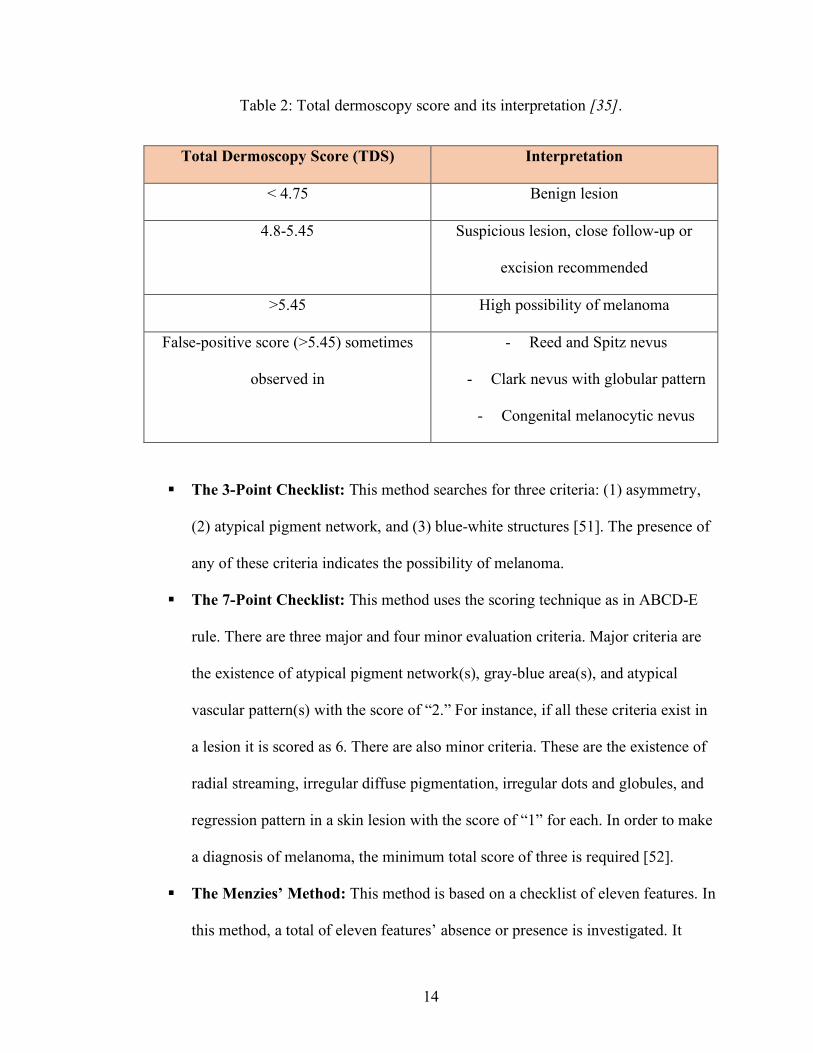
The result of TDS can be interpreted according to Table 2.

14

Table 2: Total dermoscopy score and its interpretation [35].

Total Dermoscopy Score (TDS) Interpretation

< 4.75 Benign lesion

4.8-5.45 Suspicious lesion, close follow-up or

excision recommended

>5.45 High possibility of melanoma

False-positive score (>5.45) sometimes

observed in

- Reed and Spitz nevus

- Clark nevus with globular pattern

- Congenital melanocytic nevus

§ The 3-Point Checklist: This method searches for three criteria: (1) asymmetry,

(2) atypical pigment network, and (3) blue-white structures [51]. The presence of

any of these criteria indicates the possibility of melanoma.

§ The 7-Point Checklist: This method uses the scoring technique as in ABCD-E

rule. There are three major and four minor evaluation criteria. Major criteria are

the existence of atypical pigment network(s), gray-blue area(s), and atypical

vascular pattern(s) with the score of “2.” For instance, if all these criteria exist in

a lesion it is scored as 6. There are also minor criteria. These are the existence of

radial streaming, irregular diffuse pigmentation, irregular dots and globules, and

regression pattern in a skin lesion with the score of “1” for each. In order to make

a diagnosis of melanoma, the minimum total score of three is required [52].

§ The Menzies’ Method: This method is based on a checklist of eleven features. In

this method, a total of eleven features’ absence or presence is investigated. It

15

distinguishes benign lesions from melanoma by two negative and nine positive

feature sets. The negative set includes only two features that are symmetry and

single color while the positive set includes nine features: existence of blue-white

veil, multiple brown dots, pseudopods, radial streaming, scar-like depigmentation,

peripheral black dots, multiple colors, multiple blue/gray dots, and broad pigment

network [53]. The existence of at least one feature from the positive features list

and absence of both features from the negative features list are necessary to

diagnose a lesion as malignant melanoma.

§ Pattern Analysis: Pattern analysis is another method that is used to

diagnose melanocytic lesions and to differentiate benign melanocytic lesions

from malignant melanoma. Pattern analysis method is used to identify specific

patterns of skin lesions that can be either global or local. Some of the global

patterns are reticular, globular, cobblestone, homogeneous, starburst, parallel,

multicomponent, and nonspecific, which refer to benign melanocytic lesions. The

local patterns are pigment network, dots/globules/moles, streaks, blue-whitish

veil, regression structures, hypopigmentation, blotches, and vascular structures,

which are also refer to benign melanocytic lesions [54].

16

CHAPTER 3. RELATED WORKS AND CURRENT TECHNOLOGY

For computer-assisted diagnosis of melanoma detection and malignancy

classification, we use various machine learning technologies. This chapter gives a brief

introduction to these technologies.

3.1. Overview of Machine Learning

Machine learning (ML) is an area that aims to construct new algorithms to make

predictions based on given data. ML generates general models using training data so that

these models can detect the presence or the absence of a pattern in test (new) data. In the

case of images like in this thesis, training data can be in the form of images, regions, or

pixels which are labeled or not. Patterns can be a low-level or a high-level. For instance,

a low-level pattern can be a label for pixels in segmentation while high-level pattern can

be the presence or the absence of a disease in a medical image. In this case, the image

classification becomes the addressed problem with a training set containing image-label

pairs.

3.1.1. Categories of Machine Learning Algorithms

Machine learning algorithms can be classified into three key categories based on

the different types of learning problems addressed. A list of these categories is:

§ Supervised Learning: In supervised learning, the training dataset needs to be in a

specific format. Each instance (data point) has an assigned label. Datasets are

labeled as (𝑥, 𝑦) ∈ 𝑋 × 𝑌, where 𝑥 and y denote a data point and the

corresponding true prediction for 𝑥. If the output y is part of a discrete domain,

the problem is a classification task. If the output belongs to a continuous domain,

then it is a regression task.

17

§ Unsupervised Learning: Unlike supervised learning, the datasets are not labeled

in unsupervised learning. In order to develop a structure from unlabeled data, the

ML algorithm should examine the similarities between object pairs.

§ Semi-supervised Learning: This learning task is a class of supervised learning

and uses a large amount of unlabeled data for training along with the small

amount of labeled data.

3.2. Neural Networks

Biological neural network is an important part of the human brain. It is a highly

complex system and has an ability to process different tasks simultaneously. Neural

network (NN) is a classifier that simulates the human brain and neurons. Instead of

neurons, “perceptron” is used as a basic unit of NN (see Figure 4a). NN architecture

consists of the different layers as shown in Figure 4b: (1) the input layer containing input

feature vector(s), (2) the output layer that comprises of the neural network response, and

(3) the layer containing neurons (perceptrons) between the input and output layers.

Figure 4: (a) is the perceptron layer and (b) is the image of Multi-layer Neural Network.

According to the McCulloch-Pitts model [55], the neuron k receives m input

parameter xj .The neuron also has m weight parameter wkj .The sum of inputs and weights

18

is combined and fed into an activation function j which produces the output yk of the

neuron as seen in Figure 4a. The Equation 2 below gives the mathematical understanding

of neural networks.

Equation 2

𝑦< = 𝜑∑ 𝑤<A𝑥ABACD

A neural network can learn the estimated target outputs after training by selecting the

weights of all neurons. However, it is challenging to analytically solve neuron weights of

a multi-layer network. In order to solve the weights iteratively in a simple and effective

way, the back-propagation algorithm is used. This algorithm calculates a gradient that is

needed in the calculation of the weights.

The back-propagation algorithm can be divided into two phases: propagation and

weight update. In the first phase of this algorithm, an input vector is propagated forward

through the neural network, and the output value is generated. After that, the cost (error

term) is calculated. Then, the error values are propagated back to the network to calculate

the cost of the hidden layer neurons. In the second phase of the algorithm, the neuron

weights are updated by calculating the gradient of weights and subtracting the ratio of

gradient of weights from the current weights. This ratio is called the learning rate [55].

After the update of weights, the algorithm continues with different inputs until the

weights are converged.

3.2.1. Convolutional Neural Networks

In the context of computer vision, the most commonly applied artificial neural

network is a convolutional neural network (CNN). There are two main reasons why

CNNs are used in computer vision problems. Firstly, with traditional NNs, solving the

19

computer vision problem for even relatively small sized images is challenging. For

example, a monochrome 750x563 image contains 422,250 pixels. If this image is

polychrome, the number of pixels is typically multiplied by three which is the typical

amount of color channels, and in this case, the image would have 1,266,750 pixels and

the same number of weights. Consequently, the overall number of free parameters in NN

quickly becomes extremely large which causes overfitting and reduces the performance.

Additionally, CNNs require comparatively little image pre-processing compared to other

image classification algorithms, which means CNNs can learn the filters by itself.

The CNN consists of input and output layers as well as the multiple hidden layers.

The hidden layers are usually made of convolutional layers, pooling layers, and fully

connected layers [56] (Figure 5).

§ Convolutional Layers: These layers pass the results of the input to the next layer.

It simulates the response of a neuron to visual stimuli.

§ Pooling Layers: These layers combine the outputs of neuron clusters at one layer

into a single neuron in the next layer. The purpose of this layer is to reduce the

parameters and computation in network.

§ Fully-connected Layers: These layers connect each and every neuron in one

layer to every neuron in another layer.

Figure 5: An example of a convolutional neural network [57].

20

3.3. Deep Learning and Transfer Learning

Deep learning, also known as Deep Structured Learning, is a subdivision of ML

supported by mass of algorithms. Most modern deep learning models are based on a NN,

so there is a cascade of multiple layers in deep learning similar to NNs.

Deep learning can extract useful features directly from images, text and sound in

supervised and/or unsupervised manners which makes it different than standard machine

learning techniques. In fact, feature extraction with this approach is considered as a part

of the learning process. With these characteristics of deep learning, there is less need for

hand-tuned ML solutions.

Nowadays, most applications of deep learning rely on transfer learning, especially the

domain of computer vision. Transfer learning is a ML technique where a model that is

trained on one task is repurposed on another related task. In most problems in medical

field of computer vision such as skin cancer detection, the size of the data is not big

enough (e.g., there are only thousands of images; however, CNN require much more than

that), and a lot of time is required to train a CNN from the scratch. Therefore, it is

common to use a network that is pretrained on a very large dataset (i.e., ImageNet in 1.2

million images) and then use this knowledge as an initialization for the task of interest.

There are two most common ways to apply transfer learning as follows:

§ Fixed Feature Extractor: We can use the pre-trained model as a feature

extraction mechanism. The way it works is by removing the output layer or the

last fully-connected layer and using the rest of the network as a fixed feature

extractor for the dataset of our interest.

21

§ Fine-tuning: Fine-tuning is making some fine adjustments to increase

performance further. For example, if we have one dataset, we can randomly

separate it to the training and testing (validation) dataset with the ratio of our

choice. Afterwards, we can train the model file with the training dataset and then

train the same model with the testing dataset.

22

CHAPTER 4. TEXTURE BASED SKIN LESION ABRUPTNESS

QUANTIFICATION TO DETECT MALIGNANCY

In this chapter, we introduce a novel approach to measure abrupt cutoff of pigmented

skin lesions. Abruptness of pigment patterns at the periphery of a skin lesion is one of the

most important dermoscopic features for detection of malignancy. In the current clinical

setting, abrupt cutoff of a skin lesion is determined by an examination performed by a

dermatologist. This process is subjective, nonquantitative, and error-prone. Here in this

chapter of thesis, we present an improved computational model to quantitatively measure

abruptness of a skin lesion over our previous method [58] . To achieve this, we

quantitatively analyzed the texture features of a region within the skin lesion boundary.

This region was bounded by an interior border line of the lesion boundary which is

determined using level set propagation (LSP) method. This method provides a fast border

contraction without a need for extensive boolean operations. Then, we built feature

vectors of homogeneity, standard deviation of pixel values, and mean of the pixel values

of the region between the contracted border and the original border. These vectors were

then classified using NN and SVM classifiers.

4.1. Abrupt Cutoff Measurement from Dermoscopic Images

The dataset for this part of the thesis was obtained from ISIC 2016: Skin Lesion

Analysis Toward Melanoma Detection [59], which has 900 dermoscopic images with 727

benign and 173 malignant lesions, and Edra Interactive Atlas of Dermoscopy [60], which

has 73 benign and 27 malignant lesions. The processing steps for this part of the thesis is

given in Figure 6. In this part of the thesis, we focused on border abruptness feature of

skin lesions.

23

Figure 6: Global workflow is shown.

The abrupt cutoff is a commonly accepted clinical indicator of malignancy of a

lesion. Assessment of abrupt cutoff in current clinical practice was performed by dividing

the lesion into eight virtual pieces (see Figure 7). Dermatologists searched abrupt cutoff

and assigned a score for each of the pie pieces. Since this process was carried out

manually, it led to subjective outcomes depending on the experience of the dermatologist

examining the lesion. To objectively measure and evaluate abruptness, we first

segmented the skin lesion using Boundary Driven Density Based Spatial Clustering

Application with Noise (BD-DBSCAN) algorithm [61].

24

Figure 7: (a) represent a malignant case with abrupt cutoff where the lesion is divided

into eight pieces and asterisks indicate abrupt cut off (b) represents a benign case with

gradual change at lesion border. In both cases, homogeneity feature is a strong indicator

for evaluating the abruptness.

Then, we considered the offset of a continuous function of whole lesion border via

constant velocity level sets and contracted the lesion border using these level sets. Next,

we computed texture homogeneity in the designated circular region which resides

between actual and contracted lesion border. Kaya et al. [58] was the first whose work

addresses the quantification of abruptness toward melanoma detection. In the current

study, we enhanced the prior work [38] in two aspects: i) offering a formal curve

offsetting method based on the level set propagation (LSP) which generates better and

non-overlapping contracted (inner) border [62], and ii) using NN as a classifier on an

extended data set. While the first contribution yielded us to collect more relevant data

during feature extraction, second contribution led to improved accuracy on the extended

dataset, which indicated generalizability of the developed method on a bigger dataset

over the Kaya et al. [58] method.

25

4.1.1. Boundary detection and boundary contour extraction

To access the region where abrupt cutoff possibly exists, first we need to segment the

lesion and extract the lesion border. A novel density-based clustering algorithm [61] is

used for lesion segmentation. The segmented image is recorded as black and white pixels

where black pixels are background and white pixels are foreground (refers to the lesion).

To obtain the 2D contour information of the lesion border, we use the chain-code

algorithm of Freeman [63]. The chain-code encoded a boundary in a binary

representation. These encodings referred to 8 possible directions of a neighboring pixel of

a starting pixel. These directions ranged from 0 to 7 in the rectangular-grid. Each number

refers to a transition on the direction in between two consecutive points. As can be seen

in the rectangular grid given in Figure 8 the direction numbers increase in the counter-

clockwise.

Figure 8: Chain code initialization is shown.

In chain-code, first, among all the pixels belong to foreground, the spatially

minimum pixel is selected to start the computation. The starting pixel is shown in Figure

26

9a with its minimum (X, Y) coordinates. After applying the chain code, the boundary of

the lesion is captured as depicted in Figure 9b (in green).

Figure 9: The starting point is shown in (a), and the lesion boundary is represented in

green in (b).

4.1.2. LSP for lesion border contraction

In our previous study [58], we developed a geometric model for border contraction

called dynamic scaling (DS). The nterested reader is referred to [58] for details and

mathematical foundation for the DS. In this study, however, we used level set method

[62] for border contraction. The previous method of contraction failed to provide equal

distance contraction for all the cases especially with very irregular lesion contours and

yielded unequal data collection during feature extraction. Whereas, level set based

contraction method resulted in constant proximity between original and contracted

border. These are illustrated in Figure 10a, b, c and d.

27

Figure 10: In (a) and (b), red curves represent the contracted border. (a) The curve set

shows that the LSP can obtain quantitatively accurate results. (b) The curve set shows the

DS still suffers from high curvatures and cannot offer constant distance from the original

curve. (c) shows that the DS yields a deficient data collection along the layer where the

abruptness is searched. Yellow brushes indicate that not equal amount of territory

considered for feature extraction in spanning windows. Note that, these regions are

masked using polygon intersection operations prior to feature extraction. (d) shows that

the constant velocity LSP imbues equalization of data amount during feature extraction.

Shape contraction algorithms play an important role in computer graphics, computer-

aided design, manufacturing, etc. We adopted the method studied in a seminal paper of

Kimmel et al. [24]. The following set of formulations give the details of this approach.

28

In order to formulate shape offsetting/contraction problem, let us parameterize a

curve as in the following form.

Equation 3

𝑋D(𝑠) = [𝑥(𝑠), 𝑦(𝑠)]E

where s is a curve parameterization factor for curve X0. Let us find an offset curve in a

closed form, which is expressed as,

Equation 4

𝑋F(𝑠) = 𝑋D(𝑠) − 𝑁(𝑠, 0)𝐿

Equation 4 formulates a curve leaning “parallel” to X0(s), where L is the displacement of

the offset curve, and N (s, 0) represents the unit normal at a x0(s) point and can be written

as,

Equation 5

𝑁(𝑠, 0) =1

J𝑥KL(𝑠) + 𝑦KL(𝑠)[𝑦K(𝑠), 𝑥K(𝑠)]E

where N (s, 0) is the normal of the parametric point [ys (s), xs (s)] on the curve at time 0

(e.g. N(s,0)). For instance, when L is equal to 1, displacement of each iteration will be a

single pixel. Let us consider that X (s, t) changes continuously by time (e.g., number of

iterations), hence for all t, X (s, t) = X0(s) − tN(s, 0). The term of tN (s, 0) is negative

because we do contraction; it will become positive if expansion is needed. Differential

description of this curve evolution becomes as in the following form.

Equation 6

M𝜕𝑋(𝑠, 𝑡)𝜕𝑡 = −𝑁(𝑠, 0)

𝑋(𝑠, 0) = 𝑋D(𝑠)P

29

For the first iteration t is equal to 0; thus, the curve will remain the same, which is

represented as X (s, 0) = X0 (s). Equation 6 suggests that the motion of each point on the

border (e.g., pixel) will be in inward direction (due to the contraction) of the normal as

given in Equation 7.

Equation 7

𝑁(𝑠, 𝑡) = [𝑦K(𝑠), 𝑥K(𝑠)]E1

J𝑥KL(𝑠) + 𝑦KL(𝑠)

Here the constant 1 in the numerator of the fraction refers to the velocity during the curve

propagation at time t. For faster contraction, the velocity or time step may be increased.

Equation 7 yields time t dependent shape offsets for t > 0. Figure 11b illustrates

deficiency of selecting bigger time step or higher velocity values where displacement

factor L becomes larger than the curvature. Thus, it results in loss of silhouette of actual

curvature. To overcome these possible problems (also called singularities or shocks), we

employed a more stable technique based on the flame-propagation model given in [62].

30

Figure 11: (a) Without entropy condition stability can be preserved if contraction distance

is less than the curvature of an arbitrary 2d curve; (b) Cusps emerge when contraction

distance is greater than the curvature. Shocks and cusps can be avoided adopting entropy

condition.

Shocks occur when normal of original curve collide or cross itself, in other words

when the curvature of X0 becomes singular. To address this constraint, Huygens applies

“entropy condition” on the evolving curve. Osher and Sethian [64] offered an efficient

and numerically stable wave front propagation for the curves in the plane to overcome the

self-collision problem. Osher et al. [64] applied Huygens principle, which is also known

for adhering entropy condition, proposing a solution for Equation 7 such that X(s, t) at

time t is the approximation of the whole class of disks of time t centered along the

original curve X 0(s). We adopted Osher’s method [63] with entropy condition to contract

the curve to obtain more accurate results as given in Equation 8 while eliminating the

self-collision problem. Due to the front dependency of the parameters s and t, a

Langrangian numerical-propagation scheme may be used to approximate the curve

propagation as in the following form.

31

Equation 8

⎩⎪⎨

⎪⎧𝜕𝑥(𝑠, 𝑡)

𝜕𝑡 = 𝑦K(𝑠, 𝑡)J𝑥KL(𝑠, 𝑡) + 𝑦KL(𝑠, 𝑡)

𝜕𝑦(𝑠, 𝑡)𝜕𝑡 = 𝑥K(𝑠, 𝑡)

J𝑥KL(𝑠, 𝑡) + 𝑦KL(𝑠, 𝑡)⎭⎪⎬

⎪⎫

The numerical-propagation scheme takes central derivatives of x and y in location s

and forward-derivative in time t. However, the Langrangian based numerical propagation

of a curve given in Equation 8 is unstable and suffers from the aforementioned

topological problems, i.e. shocks, self-intersections (a.k.a. self-collision). To maintain

stability and address topological problems, instead of the Langrangian numerical

propogation, we used the ‘Eulerian formulation.’

4.1.3. Eulerian Formulation Eulerian approach implements the entropy condition inherently by a recursive

procedure. Let us define a function ϕ(x, y, t) and initialize it as ϕ(x, y, t) = 0 that results in

a closed curve X(s, 0). ϕ is strictly negative inside and outside of the level

set ϕ(x, y, 0) = 0. The rationale behind this approach is to search for the surface evolution

of ϕ(x, y, t), hence level sets ϕ(x, y, t) = 0 yield the propagated curves X(s, t) preserving the

entropy condition. Let us consider ϕ(x, y, t) = 0 along X(s, t), therefore the chain rule

yields to:

Equation 9

𝜕𝑥(𝑠, 𝑡)𝜕𝑡 +

𝜕𝜑(𝑥(𝑠, 𝑡), 𝑦(𝑠, 𝑡), 𝑡)𝑥X𝜕𝑥 +

𝜕𝜑(𝑥(𝑠, 𝑡), 𝑦(𝑠, 𝑡), 𝑡)𝑦X𝜕𝑦 = 0

or

𝜑X + ∇𝑋X(𝑠, 𝑡) = 0

where

32

Equation 10

∇𝜙 = [𝜕𝜙𝜕𝑥 ,

𝜕𝜙𝜕𝑦\

represents the gradient of ∅(x, y, t) for point (x, y) at time t. The following equation is to

derive a connection with the scalar velocity of each point on the curve and its normal

direction:

Equation 11

𝜐 = 𝑵(𝑠, 𝑡). 𝑿𝒕(𝑠, 𝑡)

Here, we constrain v = 1 to have 1-pixel displacement for a single time step. Since the

gradient is always normal to the curve, it will be equal to zero as ∅(x, y, t) = 0 ; therefore,

Equation 12

𝑁(𝑠, 𝑡) = −∇𝜙‖∇𝜙‖

where negativity indicates that the direction of propagation is inward (contraction); thus,

Equation 13

𝜐 = 𝑵. 𝑿𝒕 = −∇𝜙‖∇𝜙‖𝑿𝒕 = 1

Embedding Equation 13 into Equation 9 results in the surface evolution as in the

following form.

Equation 14

𝜙X − ‖∇𝜙‖ = 0

The solution for the partial differential equation given in Equation 15 can be carried out

considering Hamilton-Jacobi Equations and gradient descent.

33

Equation 15

𝐶∆d∆e(𝑖, 𝑗) = h h i1,𝑖𝑓𝐼(𝑟, 𝑡)𝑎𝑛𝑑𝐼(𝑝 + ∆𝑥, 𝑞 + ∆𝑦) = 𝑢0,𝑜𝑡ℎ𝑒𝑟𝑤𝑖𝑠𝑒s

B

tCu

v

wCu

Algorithm 1 summarizes steps for the LSP to generate contracted border. Figure

10 illustrates results of contracted borders generated from the DS method and the LSP.

As seen from Figure 10, the LSP eliminated problems such as shocks and self-

intersections whereas these problems exist with DS. Interested readers are referred to [62]

for detailed mathematical derivations of the LSP. After contracted border is found with

LSP method, we calculated texture homogeneity between lesion border and contracted

border with various radii sizes.

Algorithm 1

• Determine a function 𝜙 (x, y, 0) such that - 𝜙(x, y, 0) = 0. yields the initial curve X(s, 0) - 𝜙(x, y, 0) < 0 represents the inside of the curve - 𝜙(x, y, 0) > 0 represents the outside of the curve - 𝜙(x, y, 0) = 0 is Lipschitz-continuous

• Propagate f on 2D grid according to 𝜙 t -||D𝜙|| = 0 • Stop the iteration after i = L/Dt time steps and select the 0-level set 𝜙(x, y, 0) = 0

which is Xt(s).

4.1.4. Feature Extraction

We obtained three different statistical measures which are mean, standard deviation,

and a texture descriptor Gray Level Co-occurrence Matrix (GLCM) as a homogeneity

indicator [65]. GLCM is a statistical method that is to analyze texture characteristics of

an image which relies on the spatial dependency of pixels. The mathematical

representation of GCLM is given below, where I is an image with nxm size, C is the co-

occurrence of intensity value u, (∆x, ∆y) is an offset parameter, and lastly r and t are the

34

spatial coordinates in the image I(r,t). Note that, offset parameters make the co-

occurrence matrix variant to rotation.

Various statistical features (texture related) could be obtained by deploying the

GCLM matrix, such as contrast, correlation, energy, and homogeneity. Here, we focused

on homogeneity which measures the similarity of grey level distribution on the image.

Hence, the homogeneity could be expressed as in the form given in Equation 16 where m

and n respectively represent the number of image pixels in the vertical and horizontal

directions. Figure 12 illustrates a sample region where homogeneity feature is extracted.

Figure 12: Homogeneity extraction from the highlighted region along the lesion

boundary.

Equation 16

h h𝐺𝐿𝐶𝑀(𝑖, 𝑗)1 + |𝑖 − 𝑗|

v

ACu

B

{Cu

After border contraction using the LSP and extracting homogeneity features in GLCM,

the next step is to analyze generated data.

4.2. Data Analysis and Results

After the feature extraction step, we categorized the dataset according to the thickness

of layer they are collected from. We selected 5, 7, 10, and 15 as the radius of circles

35

between the border and contracted border, and the layer is generated by enveloping these

circles. In each of the overlapping circles (patches), we computed the “mean

homogeneity,” “minimum homogeneity,” “mean color value average,” “minimum color

value average,” “mean color value standard deviation,” and “minimum color standard

deviation.” We performed the experiments on two different color spaces which are RGB

and HSV and fed them as input to the NN architectures and SVM.

The dataset provided dermoscopy images, which were labeled either as malignant or

benign. We were measuring abruptness of lesion along the periphery of the lesion border

using homogeneity features to conduct binary classification. Here, we argued that Multi-

layer Perceptron-based Neural Networks (MPNN) have the ability to compete with SVM

when it is combined with Softmax regression.

The hidden layer system can include multi-layers within separate instances better and

converge the values efficiently. A careful design of a NN is required for obtaining higher

accuracy rates in classification. There are some parameters that the user needs to tune

[66] for the best accuracy, such as input layer selection, weights, the number of hidden

layers, the number of nodes on each hidden layer, activation function, learning rate, the

number of iterations, and cost minimization function. We trained our NN with a pair of

input feature values and output malignancy values. In our study, in order to solve the

malignancy problem of the dataset, we chose two NN architectures: multi-layer

perceptron and the fully-connected multi-hidden layer NN. The first architecture we used

was NN model, multi-layer perceptron binary classification [67]. In this architecture, we

used a standard single layer NN which consists of an input layer, a single hidden layer,

and an output layer.

36

Figure 13 schemes the architecture. In the input layer of this NN, we used three

different inputs which are RGB channels, HSV channels, and RGB-HSV combined

channels. The number of features for RGB, HSV, and RGB-HSV channels were 18, 18,

and 36, respectively. In the hidden layer, we used the same size as they are in the input

layer. In the output layer, two classes’ values that are “benign” and “malignant” are

converted to “0” and “1,” respectively. In the running process of this NN, each epoch had

one feed forward and one back propagation. After empirical trials, execution continued at

most 1000 iterations or execution stopped when the learning rate between each epoch is

less than or equal to 0.001. The rectified linear unit (ReLU) is chosen as the activation

function for this NN.

37

Figure 13: Multi-layer Perception with a single hidden layer NN architecture.

The architecture of the second NN was fully-connected multi-hidden NN network.

Figure 14 illustrates the architecture of its design such that in this NN, the input layer

was the same with the previous NN. The hidden layer was designed with the Softmax

regression [68]. In the output layer, benign and malignant values were converted to one-

hot encodings which are [1 0] or [0 1], respectively. The implementation of this design

was done using TensorFlow NN library [69].

Input Layer Hidden Layer Output Layer

38

Figure 14: Fully-connected multi-hidden layer NN architecture.

We obtained results of two different abrupt cutoff feature extraction methods: Kaya et

al. [58] and our LSP based method using the two NN architectures introduced above with

the same parameters. Optimum results were obtained from the features collected when

radius is 10 and on RGB channel. Because NNs were highly sensitive to hyper-parameter

changes, we applied tunings to get optimum results. We empirically determined the

iteration numbers as 600, 750, and 1000 without constraining a stoppage criterion. Then,

we added the learning rate of 0.0001 to exit the iteration between two consecutive

epochs. We applied 10-fold cross-validation to split the data into training and test sets.

Since NNs generate random weights between the layers at each time, we ran the

algorithms 10 times. Consequently, all evaluation metrics are the average of the all

results generated in these experiments. Notably, to maintain consistency we used the

same dataset to test our NN designs.

We ran both NN methods and SVM on the same set of image data however different

feature vectors based on the different feature extraction methods used (the LSM and the

DS). Table 3 shows the results obtained from the multi-layer perceptron NN, fully

39

connected multi- hidden layer NN, and SVM classifiers which are fed by features

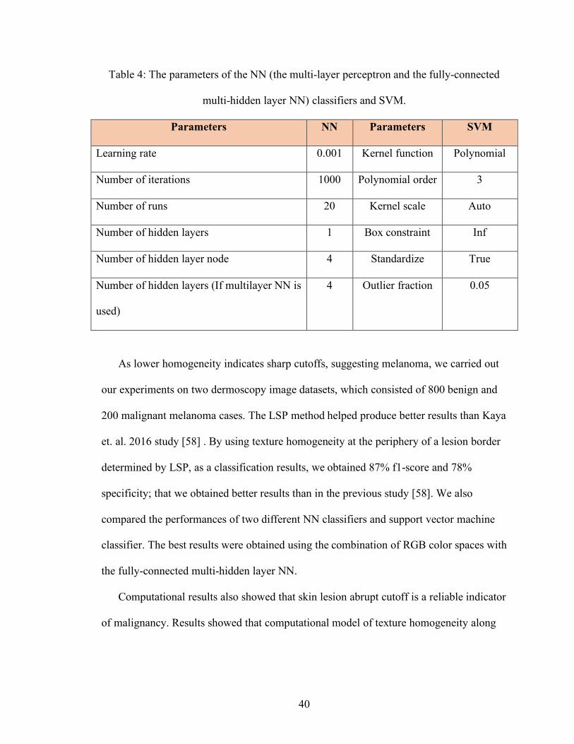
extracted using both the LSP and the DS methods. Table 4 shows the parameters of the

all classifiers used in the experiments. The highest f1-score, 87% with 78% specificity, is

obtained using fully connected multi-hidden layer NN in the RGB combination with the

radius 10.

Table 3: LSP vs. DS based texture homogeneity feature extraction and classification of

lesions with various classifiers: multi-layer perceptron, fully connected multi-hidden

layer NN, and SVM. 10-fold cross-validation is used. Results listed here are means of 10

random executions.

Feature Extraction-Classification Precision Recall Sensitivity F1-Score

LSP-Multilayer Perceptron NN 0.82 0.81 0.75 0.8

DS-Multilayer Perceptron NN 0.77 0.76 0.56 0.74

LSP-SVM 0.69 0.64 0.66 0.66

DS-SVM 0.62 0.61 0.61 0.61

LSP-Fully-connected multilayer NN 0.86 0.87 0.78 0.87

DS-Fully-connected multi-hidden layer NN 0.76 0.75 0.61 0.75

40

Table 4: The parameters of the NN (the multi-layer perceptron and the fully-connected

multi-hidden layer NN) classifiers and SVM.

Parameters NN Parameters SVM

Learning rate 0.001 Kernel function Polynomial

Number of iterations 1000 Polynomial order 3

Number of runs 20 Kernel scale Auto

Number of hidden layers 1 Box constraint Inf

Number of hidden layer node 4 Standardize True

Number of hidden layers (If multilayer NN is

used)

4 Outlier fraction 0.05

As lower homogeneity indicates sharp cutoffs, suggesting melanoma, we carried out

our experiments on two dermoscopy image datasets, which consisted of 800 benign and

200 malignant melanoma cases. The LSP method helped produce better results than Kaya

et. al. 2016 study [58] . By using texture homogeneity at the periphery of a lesion border

determined by LSP, as a classification results, we obtained 87% f1-score and 78%

specificity; that we obtained better results than in the previous study [58]. We also

compared the performances of two different NN classifiers and support vector machine

classifier. The best results were obtained using the combination of RGB color spaces with

the fully-connected multi-hidden layer NN.

Computational results also showed that skin lesion abrupt cutoff is a reliable indicator

of malignancy. Results showed that computational model of texture homogeneity along

41

the periphery of skin lesion borders based on LSP is an effective way of quantitatively

measuring abrupt cutoff of a lesion.

42

CHAPTER 5. SKIN CANCER MALIGNANCY CLASSIFICATION WITH

TRANSFER LEARNING

5.1. Introduction

Even though dermoscopy enhances the visual perception of a skin lesion,

automatic recognition of melanoma from dermoscopy images is still a difficult task, as

it has several challenges. First, the low contrast between skin lesions and normal skin

region makes it difficult to segment accurate lesion areas. Second, the melanoma and

non-melanoma lesions may have a high degree of visual similarity, resulting in the

difficulty of distinguishing melanoma lesion from non-melanoma. Third, the variation

of skin conditions, e.g., skin color, natural hairs or veins, among patients produce

different appearance of melanoma, in terms of color and texture, etc.

The misdiagnosis of a malignant skin lesion as benign (false-negative) is more

harmful than misdiagnosing a benign skin lesion as malignant (false-positive) since the

former case can become fatal due to undertreatment while the later case will just cause

over treatment (unnecessarily costly). Early detection is important for increasing the life

expectancy up to 98% compared to 17% of diagnosis in later stages [70]. Thus, there is a

need for a favorable treatment process that does an early and fast detection of skin cancer

that is vital for the patient’s life.

With this background information in mind, the purpose of our study in this chapter is

classifying and identifying skin cancer using transfer learning. Transfer learning in deep

learning is a machine learning method where a computational model developed for a task

is reused as the starting point for a model on a second task.

43

With the recent developments in image processing and classification algorithms,

researchers started using computer-aided-diagnostic systems (CAD) [71] to detect

melanoma. Also, they applied ensemble learning techniques to find the best algorithm

within the system. With the new developments on the computer vision and deep learning

algorithms, now we are able to directly import images into these algorithms and let them

automatically extract features from images by themselves. This is known as the main

difference between deep learning and machine learning. In machine learning, algorithms

learn each of the predetermined (most of the time by human) features that correlates with

the outcomes. However, machine learning cannot influence the way that the features are

defined. Whereas in deep learning, a good set of features are algorithmically captured (it

learns features itself).

Transfer learning is one of the most popular techniques on computer vision and deep

learning field to transfer knowledge from one domain to another. Transfer learning

allows users to utilize pretrained weights from another domain in case of limited

computational power.

In this study, we used Inception v3 image classification transfer learning algorithm

[12] with pretrained ImageNet dataset weights to solve the complexity of skin lesions

and to classify skin lesions in dermoscopy images according to their malignancy. The

dataset for this study was obtained from the International Skin Imaging Collaboration

(ISIC) [11]. In order to eliminate a possible bias problem, we randomly selected dataset

images for training and testing and used them for various experiments.

44

5.2. Dermoscopy Image Preprocessing

The optical lenses of digital cameras reduce the quality of the digital images of skin

lesions. This causes some difficulties in the diagnosis of malignancy by visual assessment

due to the complexity of digital images. Therefore, there is a need for efficient image

processing techniques to help physicians diagnose skin lesions accurately. Image pre-

processing makes images suitable for this application by improving the quality of an

image and for manipulating datasets by removing the noise and irregularities present in

an image [72, 73]. In this study, the training set contained more than 13,000 skin lesion

images of different resolutions [11]. Because the resolution of all lesion images is greater

than 299 x 299, it was necessary to extract the region of interest (skin lesion) and get rid

of unnecessary/redundant regions from each image. Thus, we automatically cropped and

processed these images before using in the image classification algorithm. This

preprocessing step is necessary for; first, reducing the computation time by

removing/reducing number of pixels to be processed; second, increasing performance of

the classifier. Image pre-processing steps used in this study are segmentation, auto-

cropping, and image resampling.

5.2.1. Image Segmentation

Image segmentation is a process of dividing an image into multiple segments that are

considerably/perceptually homogeneous in terms of preferred characteristics such as

color, texture, etc. Image segmentation is typically used to identify objects, estimate the

boundaries of an image, remove unwanted regions on the image, compress and edit

images or manipulate and visualize the data [74, 75] with a goal of providing a

45

description or classification of the image. This process is widely used especially in

medical image processing.

We start segmentation process by first finding the superpixels. Superpixels are one of

the most popular images over-segmentation algorithms. Among many superpixel

algorithms, the choice of superpixel algorithm in this thesis is Simple Linear Iterative

Clustering (SLIC) [76]. SLIC is categorized as a gradient ascent method and it is often

used as a baseline [77, 78]. SLIC implements a local K-means clustering to generate a

superpixel segmentation with K-superpixels. More specifically, it groups similar pixel

values and improves superpixel centers [79] using K-means clustering algorithm. In our

case, we use SLIC to automatically detect the region of interest (skin lesion) and use that

to automatically crop the image without losing a part of a skin lesion. The original skin

lesion images (i.e., Figure 15a) were divided to 400 superpixel areas (dynamically

determining each super pixel size of 16 x 16) (Figure 15b), which are separated by blue

lines. We empirically found that starting with 400 superpixel centers is optimal.

Figure 15: Example of superpixels. The original image (a) was subdivided to 400

superpixel areas (b) separated by blue lines.

46

The next step is roughly extracting the entire the skin lesion. To do that, we needed to

find a way to merge superpixels that include some part of the lesion. For merging

superpixels, we considered using some segmentation techniques including thresholding

technique, edge detection technique, region extraction technique, and fuzzy-based image

segmentation [80, 81]. To merge superpixels that fall partially or entirely in skin lesion

region, we used thresholding technique and merging superpixels.

The next step is automatically cropping the image.

5.2.2. Cropping and Image Resampling

Image resampling is a technique used to manipulate the size of an image. Increasing

the size of the image is called upsampling while decreasing the size is called

downsampling. These two techniques are essential for applications like image display,

compression, and progressive transmission [82]. During downsampling or upsampling

processes, a two-dimensional (2D) representation is kept the same while the spatial

resolution is reduced or increased, respectively. On the other hand, cropping is a

technique used to find the region of interest in an image by framing around and clipping

the area. Figure 16 illustrates all the preprocessing steps in order.

47

Figure 16: Images after each preprocessing steps: (a) is the original image obtained from

ISIC 2018 Challenge, (b) is the segmentation mask of the image, (c) is the overlap of (a)

and (b), (d) is framing the Region of Interest, and (e) is the cropped and resized to n x n

image.

5.2.3. Image Resizing with Adding Zero-Padding

The data obtained from the ISIC archive [11] is not always available to directly feed

the algorithm which requires structures, clean and meaningful data. In order to overcome

this problem, we resized all images from the archive to 299x299 without losing any

feature. Pseudo-code for this process is as follows:

1- Identify which side of the image is short.

2- Find the difference between two sides.

3- Take half of the difference.

4- Do padding by putting number of zeros to short sides by adding half of the

difference.

5- Resize the image to 299x299.

48

After the skin lesion is roughly extracted from the dermoscopy images, the next step

is classifying these lesions.

5.3. Classification

Classification can be defined as making groups of things based on shared features,

characteristics or other predefined properties. During the training phase, feature values of

images are extracted from dermoscopy images of skin lesions for estimating the classes

of images in test sets. There is one label for each image.

There are several most popular algorithms to solve classification problems such as

decision trees, neural networks (NN), and support vector machines (SVM). However,

these algorithms require manual feature extraction and preprocessing, and they can only

calculate numeric values. In order to pass these cumbersome steps and make the

algorithm do the feature extraction itself, we used transfer learning algorithm Inception

V3 that is a specialized version of convolutional neural network. By transferring

previously gained knowledge, we drastically reduced overall computation time without

sacrificing efficiency. The architecture of the algorithm is shown in Figure 17.

Figure 17: Google Inception v3 transfer learning algorithm layers [83].

49

There are other several convolutional neural network architectures such as AlexNet

[84], VGGNet [85], and ResNet [86]. Because training these architectures requires big

data and is a computationally intensive process, excessive computation power (GPU

power) is needed. Also, since we use a supervised technique, training data sets need to

have verified labels. In order to label these large datasets, crowd sourcing or community

driven labelling methods should be used. Finding these datasets is also one of the

difficulties of classification process.

In the skin cancer field, the most popular crowd sourced data is the International Skin

Imaging Collaboration (ISIC). The ISIC has expert-labelled datasets, and the number of

images constantly increases. Most skin cancer researchers use the ISIC dataset to test the

performance of their algorithms.

5.4. Experiments and Performance Analysis

The ISIC dataset has reached over 23,900 skin lesion images which were labeled by

expert physicians according to their types of malignancy by the date of July 8, 2018.

There were 19,373 benign and 2,286 malignant images. These images had descriptions

about patients’ anonymized data.

We used 12,600 benign and 1,084 malignant images on our first experiment (The

number of images in the ISIC dataset was around 13,700 at the time). In this case, images

were not preprocessed before feeding the algorithm. The purpose was examining the

performance of Inception v3 algorithm based on the existence of the noise and other

artifacts to see how much it tolerates the noise. Images were randomly split into training

and testing subsets. The training set had 12,500 benign and 984 malignant images. On the

testing set, there were 100 benign and 100 malignant images, and we did this testing with

50

ten different 100 benign and 100 malignant pairs. These sets were randomly selected in

order to eliminate bias. The classification report for the first experiment is displayed

below (Table 5). Notice that we obtained 0.89 f1 score (89%) for malignancy accuracy.

Table 5: Results of experiment 1 with 13684 images.

Class Number Precision Recall F1-Score Support

(Benign)-0 0.96 0.79 0.87 100

(Malignant)-1 0.82 0.97 0.89 100

Average / Total 0.89 0.88 0.88 200

The classification report displays precision, recall, f1-score, and number of images

per class which were listed as support values. Class numbers were represented with “0”

for benign and “1” for malignant. On the third line of the report, average precision, recall,

and f1-score values with total images on testing set are displayed.

F1-score is a good indicator for performance measuring of classification algorithms.

According to our classification result, malignant class f1-score was higher than benign

class. This was a good indication of how well the algorithm handled the malignant cases;

however, there was overfitting and an imbalanced data problem in the experiment.

One of the common problems on machine learning algorithms is the imbalanced data

problem. The imbalanced data problem is caused by the ununiform class distribution.

This problem was predominant in scenarios where anomaly detection was crucial as in

51

our case. In our study, the imbalanced data problem corresponds to the percentage of the

malignant images over benign images, which is 8.6%. There are many approaches to

solving imbalanced data problems, such as decreasing the number of benign images to

the malignant image number, collecting more malignant data, or data augmentation, etc.

Collecting more malignant images was not an option for our case because we were

dependent on the ISIC archive. When we were studying on this problem, the number of

images for malignant cases in the ISIC archive was only 1,084. In order to solve the

imbalanced data problem, we decreased the number of benign images around to the

number of malignant images. The next experiment set up and results are explained in the

following paragraphs.

In the second experiment, we used 984 malignant and 1,000 benign images for

training, and 100 malignant and 100 benign images for testing. We randomly split images

into their training and testing subsets as fine-tuning process.

Table 6: Results of experiment 2 with 1,984 images using transfer learning.

Class Number Precision Recall F1-Score Support

(Benign)-0 0.91 0.79 0.84 100

(Malignant)-1 0.81 0.92 0.86 100

Average / Total 0.86 0.85 0.85 200

52

As it is seen from the classification report (Table 6), the values for all columns and

average values were lower than the previous experiment (experiment 1). However,

malignant class (class ID 1) had a higher recall and an f1-score values on this experiment

which is close to the first experiment. The result of this experiment showed that lowering

the number of benign images was not a good idea for solving the imbalanced data

problem.

Thus, in the third experiment, we considered including previously mentioned

(keeping the hyper-parameters and the experiment setup the same). With this motivation,

we identified false predicted images on the first experiment and manually cropped them

to eliminate noise, hair, water, and the other artifacts around the region of interest. After

this, we trained the classification algorithm again by adding cropped versions of false

predicted images. After many trials for fine tuning and the optimum outcome, we

obtained the results given in Table 7, which were the best results so far.

Table 7: Results of experiment 3 with 13,684 images using transfer learning.

Class Number Precision Recall F1-Score Support

(Benign)-0 0.93 0.84 0.88 100

(Malignant)-1 0.85 0.94 0.90 100

Average / Total 0.89 0.89 0.89 200

53

Compared to the first experiment, Table 7 showed higher recall and f1-score

average values. This indicated that the image preprocessing step had a profound impact

on the classification algorithm by making the region of interest more clean,

distinguishable, obvious, and easy to capture so that the algorithm could extract better

features about the image and learned better.

With this motivation, we decided to conduct an experiment on the image

segmentation algorithm to segment skin lesions before importing them to the training

phase of the image classification algorithm. We used the SLIC superpixel algorithm that

is described in the previous section. In order to find the region of interest, we tried the

thresholding technique, which is determining the threshold value and applying it to all

superpixels. If the superpixel value was higher than or equal to the threshold value, we

considered it as a part of the region of interest. We first found the mean average values of

all super pixels. Then, we selected their standard deviation value and applied it as a

threshold value to all super pixels. The result was not optimal to extract only the region

of interest. Then, we considered the median value of all super pixels as the threshold

value. With the median value as a threshold, we were able to get a better result than what

physicians draw. The result of the median threshold method is displayed on Figure 18c.

54

Figure 18: (a) is the original image, (b) is the segmentation mask drawn by a physician, (c) the segmentation mask that is the result of our segmentation algorithm.

Skin lesion images were observed mostly with some noise or other unwanted artifacts

around. This situation made us develop another way of pre-processing the images. In the

first experiment, we fed the classifier algorithm with raw images, which means that we

did not crop or resize them, but the algorithm handled this for us. The algorithm

randomly selected a pixel, adding a 299x299 window on it and finally cropping. This

showed that the algorithm could learn only with a random piece of an image. What if we

gave the algorithm an actual image resized to 299x299 before feeding into the algorithm?

With this way, we could keep all the features of an image and help the algorithm to do an

enhanced feature extraction not only using skin lesion information but also the entire skin

in the image.

55

The Inception v3 image classification algorithm is a noise-tolerable algorithm that

we saw on the first three experiments. On the next experiment, we fed the algorithm with

the pre-processed images before the training step.

In the fourth experiment, we used a larger malignant dataset with the size of 2,286

malignant images and the same number of benign images as the number of images on the

ISIC archive has been increased. The reason was that the Inception v3 classification

algorithm could not handle the imbalanced data problem by itself. We manually arranged

the number of images before training it.

In this stage of the study, we resized all of the images to 299x299 by adding zero-

pixel values to the short side. With this way, we kept features of the skin lesions and also

let the algorithm learn the skin lesion malignancy with its skin color.

Figure 19: Square malignant image after resizing process.

Figure 19 shows the square image we had after adding zero-pixel values to the short

side of the image, which is the top and bottom portions of the image in this example.

After the resizing step, we randomly split images into training and testing subsets. 2,086

malignant and 2,086 benign images were in training set, and 200 malignant and 200

benign images were on testing sets. Notice that now the data is balanced. We fed the

56

algorithm with these image sets and fine-tuned it to get optimum results. The results of

this experiment are shown in Table 8.

Table 8: Results of the experiment 4.

Class Number Precision Recall F1-Score Support

(Benign)-0 0.97 0.92 0.94 200

(Malignant)-1 0.92 0.97 0.95 200

Average / Total 0.95 0.94 0.94 400

The classification results of experiment four were the best overall in all

categories. Similar to the first two experiments, malignant class’ f1-score was again

higher than the benign class. Training and validation iteration results are illustrated in

Figure 20. This plot indicates that results are reproducible, and the algorithm is robust

and reliable with high confidence for accurately classifying lesions as benign or

malignant.

57

Figure 20: Accuracies of training and validation for each iteration.

These results also indicate that there is no overfitting or underfitting on the transfer

learning model. Also, we examined the cross-entropy loss (log loss) which measures the

performance of a classification model whose output is a probability value between 0 and

1. As predicted, probability diverges from the actual label, cross-entropy loss increases. A

perfect model would have a log loss of 0.

In this experiment, results were very similar to each other. Cross entropy loss plot is

displayed in Figure 21. Cross entropy loss values were in the border of 0.1 which is very

close to a perfect model. With this fine-tuning and configuration, the Inception v3 image

classification algorithm gave very accurate results on classification of the skin lesions

from dermoscopy images.

Figure 21: Cross-entropies of training and validation.

58

5.5. Discussion

Irregular shapes of skin lesions, different types of colors on each skin, and

determining the region of interest on each dermoscopy image are just a few challenges in

skin cancer detection. Detecting minute changes on the skin requires expertise in this

field. However, the human eye may not always catch these tiny changes. Helping doctors

with the computer vision and deep learning techniques can save many lives. With this

motivation, we studied skin cancer malignancy detection to classify skin lesions and

identify malignant cases. Pre-training settings and post-training measurements of all

experiments showed that the skin cancer malignancy detection is a difficult task and

generalizing a model for all cases requires some image preprocessing techniques to apply

before feeding into any deep learning algorithm. We did many experiments and tried

various techniques to solve the complexity of skin lesions classes. Finally, we were able

to classify skin lesions with 94% average f1-score. Also, the malignant class skin

classification f1-score (95%) was higher than benign class f1-score. This result is a good

indicator for the potential of such a technology to reduce false-negative and false-positive

predictions and eventually help physicians increase their diagnostic prediction power.

59

CHAPTER 6. CONCLUSIONS

Skin cancer is increasing and affects many people every day. This cancer can be

treated successfully if it is detected in early stages. Early diagnosis and treatment will

lead to an increased survival chance and reduced mortality rates. However, current

clinical techniques used for the diagnosis of malignant melanoma are prone to human

error due to the subjectivity and novice physicians. Therefore, there is a need for more

reliable and accurate systems that can be beneficial to both expert and novice physicians.

This thesis proposed creative and effective methods to eliminate the subjectivity in

visual interpretation of dermoscopy images and decrease the number of false-

negative/false-positive diagnoses by introducing a new method for measuring abrupt

cutoff and increasing the performance of feature extraction algorithms. There are two

main studies done in this thesis: (1) skin lesion abruptness quantification, and (2) skin

lesion malignancy classification using transfer learning.

6.1. Skin Lesion Abruptness Quantification

Abruptness of pigments on the skin is one of the most important dermoscopic features

for detection of malignancy. In the current clinical setting, abruptness is determined by an

examination performed by a dermatologist. This process is subjective, non-quantitative,

and error-prone. We presented an improved computational model to quantitatively

measure abruptness of a skin lesion by quantitatively analyzing the texture features of a

region within the lesion boundary. This region was bounded by an interior border line of

the lesion boundary which is determined using the level set propagation (LSP) method.

This method provided a fast border contraction without a need for extensive boolean

operations. Then, we built feature vectors of homogeneity, standard deviation of pixel

60

values and mean of the pixel values of the region between the contracted border and the

original border. These vectors were then classified using neural networks (NN) and SVM

classifiers. By using texture homogeneity at the periphery of a lesion border determined

by LSP, as a classification results, we obtained 87% f1-score and 78% specificity.

6.2. Skin Lesion Classification using Transfer Learning

Misdiagnosis of malignant melanoma is the real reason of fatality due to skin cancer.

Even though there are imaging and diagnosis techniques used commonly for melanoma

like dermoscopy, automatic recognition is still challenging due to the difficulty of

segmenting accurate lesion areas, similarity between melanoma and non-melanoma

lesions and the variation of skin conditions. Besides these problems, medical images are

not easy to find while protecting the anonymity of the patients. Since there were not

enough images of melanoma cases to properly train datasets, we used Inception v3 image

classification transfer learning algorithm with pretrained ImageNet dataset weights.

Before applying image preprocessing steps prior to feeding the algorithm, we obtained

89% f1-score for malignant cases. However, after feeding the algorithm with the resized

and preprocessed images, we were able to acquire 95% of f1-score for malignant cases.

To sum up, the objectives of this thesis were to eliminate the subjectivity on visual

interpretations of dermoscopy images for abrupt cutoff and to reduce the number of false-

negative/false-positive diagnosis of malignancy classification.

61

REFERENCES

[1] "Cancer Facts and Figures," 2010. [Online]. Available: http://www.cancer.org/Research/CancerFactsFigures/CancerFactsFigures/cancer-factsand-figures-2010.. [Accessed June 2018].

[2] "Melanoma," [Online]. Available: https://www.cancer.org.au/about-cancer/types-of-cancer/skin-cancer/melanoma.html. [Accessed June 2018].

[3] "Early diagnosis of malignant melanoma," [Online]. Available: https://www.clinicaladvisor.com/features/early-diagnosis-of-malignant-melanoma/article/305429/. [Accessed July 2018].

[4] M. Celebi, Y. Aslandogan, W. Stoecker, H. Iyatomi, H. Oka and X. Chen, "Unsupervised border detection in dermoscopy images," Skin Research and Technology, vol. 13, no. 4, pp. 454-462, 2007.

[5] M. Fleming, C. Steger and e. al., "Techniques for a structural analysis of dermatoscopic imagery," Computerized Medical Imaging and Graphics, vol. 22, no. 5, pp. 375-389, 1998.

[6] G. Argenziano, H. Soyer and e. al., "Dermoscopy of pigmented skin lesions: results of a consensus meeting via the internet," Journal of the American Academy of Dermatology, vol. 48, no. 5, pp. 679-693, 2003.

[7] R. Kenet and T. Fitzpatrick, " Reducing mortality and morbidity of cutaneous melanoma: a six year plan. b). identifying high and low risk pigmented lesions using epiluminescence microscopy," The Journal of Dermatology, vol. 21, no. 11, pp. 881-884, 1994.

[8] S. Menzies, C. Ingvar, K. Crotty and e. al., "Frequency and morphologic characteristics of invasive melanoma lacking specific surface microscopy features," Archives of Dermatology, vol. 132, pp. 1178-1182, 1996.

[9] H. Pehamberger, A. Steiner and K. Wolff, " In vivo epiluminescence microscopy of pigmented skin lesions. i. pattern analysis of pigmented skin lesions," Journal of the American Academy of Dermatology, vol. 17, no. 4, pp. 571-583, 1987.

[10] G. Argenziano, G. Fabbrocini, P. Carli, V. De Giorgi, E. Sammarco and M. Delfino, "Epiluminescence microscopy for the diagnosis of doubtful melanocytic skin lesions: Comparison of the ABCD fule of dermatoscopy and a new 7-point checklist based on pattern analysis," Archives of Dermatology, vol. 134, no. 12, pp. 1563-1570, 1998.

[11] "International Skin Imaging Collaboration Archive," [Online]. Available: https://isic-archive.com/. [Accessed 2018].

[12] C. Szegedy, V. I. S. Vanhoucke, J. Shlens and Z. Wojna, "Rethinking the Inception Architecture for Computer Vision," arXiv:1512.00567, 2015.

[13] "World Health Organization," [Online]. Available: http://www.who.int/en/.. [Accessed June 2018].

[14] "Cancer Projected To Become Leading Cause Of Death Worldwide In 2010," [Online]. Available:

62

https://www.sciencedaily.com/releases/2008/12/081209111516.htm. [Accessed July 2018].

[15] E. Proksch, J. Brandner and J. Jensen, "The skin: an indispensable barrier," Experimental Dermatology, vol. 17, no. 12, pp. 1063-1072, 2008.

[16] K. Madison, ""Barrier function of the skin: "la raison d'être" of the epidermis"," J Invest Dermatol, vol. 121, no. 2, pp. 231-241, 2003.

[17] M. Stücker, A. Struk, P. Altmeyer, M. Herde, H. Baumgärtl and D. Lübbers, "The cutaneous uptake of atmospheric oxygen contributes significantly to the oxygen supply of human dermis and epidermis," The Journal of Physiology, vol. 538, no. 3, pp. 985-994, 2002.

[18] "CancerHelp," [Online]. Available: http://cancerhelpessentiahealth.org/Cancer_Types/melanoma_201302E2_01.html. [Accessed July 2018].

[19] "Cancer Facts & Figures," 2013. [Online]. Available: http://www.cancer.org/acs/groups/content/@epidemiologysurveilance/documents/docu ment/acspc-036845.pdf.. [Accessed July 2018].

[20] "What Is Cancer?," June 2014. [Online]. Available: https://web.archive.org/web/20140625220940/http://www.cancer.gov/cancertopics/cancerlibrary/what-is-cancer. [Accessed July 2018].

[21] F. M. Walter, A. T. Prevost, J. Vasconcelos, P. N. Hall, N. P. Burrows, H. C. Morris, A. L. Kinmonth and J. D. Emery, "Using the 7-point checklist as a diagnostic aid for pigmented skin lesions in general practice: a diagnostic validation study," Br J Gen Pract, vol. 63, no. 610, pp. 345-353, 2013.

[22] N. di Meo, G. Stinco, S. Bonin, A. Gatti, S. Trevisini, G. Damiani, S. Vichi and G. Trevisan, "CASH algorithm versus 3-point checklist and its modified version in evaluation of melanocytic pigmented skin lesions: the 4-point checklist," J Dermatol, vol. 6, pp. 682-685, 2016.

[23] M. Celebi, H. Kingravi, B. Uddin, H. Iyatomi, Y. Aslandogan, W. Stoecker and R. Moss, " A methodological approach to the classification of dermoscopy images," Comput Med Imaging Graph., vol. 31, no. 6, pp. 362-373, 2007.

[24] S. Dreiseitl, L. Ohno-Machado, H. Kittler, S. Vinterbo, H. Billhardt and M. Binder, "A comparison of machine learning methods for the diagnosis of pigmented skin lesions," J Biomed Inform, vol. 34, no. 1, pp. 28-36, 2001.

[25] P. Rubegni, G. Cevenini, M. Burroni, R. Perotti, G. Dell'Eva, P. Sbano, C. Miracco, P. Luzi, P. Tosi, P. Barbini and e. al, "Automated diagnosis of pigmented skin lesions," Int J Cancer, vol. 101, no. 6, pp. 576-580, 2002.

[26] H. Iyatomi, H. Oka, M. Celebi, M. Hashimoto, M. Hagiwara, M. Tanaka and K. Ogawa, "An improved internet-based melanoma screening system with dermatologist-like tumor area extraction algorithm," Comput Med Imaging Graph, vol. 32, no. 7, pp. 566-579, 2008.

[27] N. Situ, X. Yuan and G. Zouridakis, "Malignant melanoma detection by bag-of-features classification," in 2008 30th annual international conference of the IEEE engineering in medicine and biology society, 2008.

63

[28] W. V. Stoecker, M. Wronkiewiecz, R. Chowdhury, R. J. Stanley, J. Xu, A. Bangert, B. Shresta, D. A. Calcara, H. S. Rabinovitz and M. Oliviero, "Detection of granularity in dermoscopy images of malignant melanoma using color and texture features," Comput. Med. Imaging Graph, vol. 35, no. 2, pp. 144-147, 2011.

[29] G. Fabbrocin, G. Betta, G. Leo, C. Liguor, A. Paolillo, A. Pietrosanto, P. Sommella, O. Rescigno, S. Cacciapuoti, F. Pastore, V. Vita, I. Mordente and F. Ayala, "Epiluminescence image processing for melanocytic skin lesion diagnosis based on 7-point check-list: a preliminary discussion on three parameters," Open Derm J, vol. 4, pp. 110-115, 2010.

[30] W. Stoecker, K. Gupta, R. Stanley, R. Moss and B. Shrestha, "Detection of asymmetric blotches (asymmetric structureless areas) in dermoscopy images of malignant melanoma using relative color.," Skin Res Technol., vol. 11, no. 3, pp. 179-184, 2005.

[31] M. Celebi, H. Iyatomi, W. Stoecker, R. Moss, H. Rabinovitz, G. Argenziano and H. Soyer, "Automatic detection of blue-white veil and related structures in Dermoscopy images.," Comput Med Imaging Graph, vol. 32, no. 8, pp. 670-677, 2008.

[32] G. Leo, A. Paolillo, P. Sommella and G. Fabbrocini, "Automatic diagnosis of melanoma: a software system based on the 7-point check-list.," in 2010 43rd Hawaii international conference on system sciences, Hawaii, 2010.

[33] S. Seidenari, G. Pellacani and C. Grana, "Pigment distribution in melanocytic lesion images: a digital parameter to be employed for computer-aided diagnosis," Skin Res Technol, vol. 11, no. 4, pp. 236-241, 2005.

[34] M. Burroni, P. Sbani, G. Cevenini, M. Risulo, G. Dell'Eva, P. Barbini, C. Miracco, M. Fimiani, L. Andreassi and P. Rubegni, "Dysplastic naevus vs. in situ melanoma: digital dermoscopy analysis," Br J Dermatol., vol. 152, no. 4, pp. 679-684, 2005.

[35] F. Nachbar, W. Stolz, T. Merkle, A. B. Cognetta, T. Vogt, M. Landthaler, P. Bilek, O. Braun Falco and G. Plewig, "The ABCD rule of dermatoscopy: High prospective value in the diagnosis of doubtful melanocytic skin lesions," Journal of the American Academy of Dermatology, vol. 30, no. 4, pp. 551-559, 1994.

[36] R. Stanley, W. Stoecker and R. Moss, "A relative color approach to color discrimination for malignant melanoma detection in dermoscopy images," Skin Res Technol, vol. 13, no. 1, pp. 62-72, 2007.

[37] Y. Faziloglu, R. Stanley, R. Moss, W. Stoecker and R. McLean, "Colour histogram analysis for melanoma discrimination in clinical images," Skin Res Technol, vol. 9, no. 2, pp. 147-156, 2003.

[38] "Cancer Facts and Statistics 2015," [Online]. Available: https://isic-archive.com/. [Accessed March 2016].

[39] R. Siegel, K. Miller and A. Jemal, "Cancer Statistics," CA Cancer J Clin., vol. 67, no. 1, pp. 7-30, 2017.

[40] M. O. Caroline and R. T. Nicholas, "Skin Cancer," Medicine, vol. 33, no. 1, pp. 64-67, 2005.

[41] R. Gordon, "Skin Cancer: An Overview of Epidemiology and Risk Factors," Seminars in Oncology Nursing, vol. 29, no. 3, pp. 160-169, 2013.

64

[42] "World Cancer Report," World Health Organization, 2014. [43] "Melanoma Treatment for Health Professionals," July 2015. [Online]. Available:

https://web.archive.org/web/20150704213842/http://www.cancer.gov/types/skin/hp/melanoma-treatment-pdq. [Accessed July 2018].

[44] "Basal Cell Carcinoma (BCC)," [Online]. Available: https://www.skincancer.org/skin-cancer-information/basal-cell-carcinoma. [Accessed July 2018].

[45] B. Cakir, P. Adamson and C. Cingi, "Epidemiology and economic burden of nonmelanoma skin cancer," Facial Plastic Surgery Clinics of North America, vol. 20, no. 4, pp. 419-422, 2012.

[46] "Squamous Cell Carcinoma (SCC)," [Online]. Available: https://www.skincancer.org/skin-cancer-information/squamous-cell-carcinoma/scc-warning-signs-and-images#panel1-1. [Accessed July 2018].

[47] T. DiChiara, "Pictures of Moles and Melanoma skin cancer – Learn o tell the difference with pictures.”," 2010.

[48] B. Hibler, Q. Qi and A. Rossi, "Current state of imaging in dermatology," Seminars in Cutaneous Medicine and Surgery, vol. 35, no. 1, pp. 2-8, 2016.

[49] M. P.-S. S. A. K. H. M. M. Binder, A. Wolff, H. Pehamberger and A. Austria, "Epiluminescence Microscopy. “A useful tool for the diagnosis of pigmented lesions for formally trained dermatologists"," Journal of the American Academy of Dermatology, vol. 36, no. 2, pp. 286-291, 1997.

[50] P. Kittler H, K. Wolff and M. Binder, "Diagnostic accuracy of dermoscopy.," Lancet Oncol, vol. 3, pp. 159-165, 2002.

[51] G. Argenziano, "3 Point Checklist of Dermoscopy," 2006. [52] "7-Point Checklist," [Online]. Available: https://dermlite.com/pages/7-point-checklist.

[Accessed July 2018]. [53] "Menzies Method," [Online]. Available: https://dermoscopedia.org/Menzies_Method.

[Accessed July 2018]. [54] A. Masood, Developing Improved Algorithms for Detection and Analysis of Skin

Cancer, 2016. [55] C. Bishop, "Pattern Recognition and Machine Learning," Information Science and

Statistics, 2006. [56] M. Thoma, Analysis and Optimization of Convolutional Neural Network

Architectures, Department of Computer Science, FZI Research Center of Information Technology, 2017.

[57] O. Stenroos, Object detection from images using convolutional neural networks, Espoo: School of Science, Aalto University, 2017.

[58] S. Kaya, M. Bayraktar, S. Kockara, M. Mete, T. Halic, H. Field and H. Wong, "Abrupt skin lesion border cutoff measurement for malignancy detection in dermoscopy images," BMC Bioinformatics, vol. 17, no. 13, p. 367, 2016.

[59] D. Gutman, N. Codella, E. Celebi, B. Helba, M. Marchetti, N. Mishra and A. Halpern, "Skin Lesion Analysis toward Melanoma Detection: A Challenge at the International

65

Symposium on Biomedical Imaging (ISBI) 2016," in International Skin Imaging Collaboration (ISIC). CoRR 2016.

[60] P. Lio and P. Nghiem, "Interactive Atlas of Dermoscopy," J Am Acad Dermatol, vol. 50, no. 5, pp. 807-808, 2004.

[61] M. Mete and N. Sirakov, "Lesion detection in demoscopy images with novel density-based and active contour approaches.," BMC Bioinformatics, vol. 11, no. 6, pp. 6-23, 2010.

[62] R. Kimmel and A. Bruckstein, "Shape offsets via level sets," Comput Aided Des, vol. 25, no. 3, pp. 154-162, 1993.

[63] H. Freeman, "On the encoding of arbitrary geometric configurations," IRE Transactions on Electronic Computers EC- 10, pp. 260-268, 1961.

[64] S. Osher and J. A. Sethian, "Fronts propagating with curvature-dependent speed: algorithms based on Hamilton-Jacobi formulations," J Comput Phys., vol. 79, no. 1, pp. 12-49, 1988.

[65] R. M. Haralick, K. Shanmugam and I. Dinstein, "Textural features for image classification," IEEE Trans Syst Man Cybern., Vols. SMC-3, no. 6, pp. 610-621, 1973.

[66] Y. LeCun, L. Bottou, G. B. Orr and K. Muller, "Efficient backprop," Neural networks: Tricks of the trade, pp. 9-48, 2012.

[67] F. Pedregosa, G. Varoquaux, A. Gramfort, V. Michel, B. Thirion, O. Grisel, M. Blondel, P. Prettenhofer and e. al., "Sci-kit learn: machine learning in Python," J Mach Learn Res, vol. 12, pp. 2825-2830, 2011.

[68] "Softmax Regression," [Online]. Available: http://ufldl.stanford.edu/wiki/index.php/Softmax_Regression. [Accessed 9 November 2017].

[69] M. Abadi, P. Barham, J. Chen, Z. Chen, A. Davis, J. Dean, M. Devin, S. Ghemawat, G. Irving, M. Isard and e. al., "TensorFlow: a system for large-scale machine learning," in OSDI'16 Proceedings of the 12th USENIX conference on Operating Systems Design and Implementation, Savannah, GA, 2016.

[70] R. L. Siegel, K. D. Miller and A. Jemal, "Cancer statistics," A Cancer Journal for Clinicians, vol. 66, no. 1, pp. 7-30, 2016.

[71] K. Møllersen, H. Kirchesch, M. Zortea, T. Schopf, K. Hindberg and F. Godtliebsen, "Computer-Aided Decision Support for Melanoma Detection Applied on Melanocytic and Nonmelanocytic Skin Lesions: A Comparison of Two Systems Based on Automatic Analysis of Dermoscopic Images," Biomed Research International, vol. 2015, 2015.

[72] N. Ponraj, M. E. Jenifer, P. Poongodi and J. S. Manoharan, "A Survey on the Preprocessing Techniques of Mammogram for the Detection of Breast Cancer," Journal of Emerging Trends in Computing and Information Sciences, vol. 2, no. 12, pp. 656-664, 2011.

[73] B. Chitradevi and P. Srimathi, "An Overview on Image Processing Techniques," International Journal of Innovative Research in Computer and Communication Engineering, vol. 2, no. 11, pp. 6466-6472, 2014.

66

[74] A. D. Jepson and D. J. Fleet, "Image Segmentation," 2007. [Online]. Available: http://www.cs.toronto.edu/~jepson/csc2503/segmentation.pdf. [Accessed June 2018].

[75] "Image Segmentation," [Online]. Available: https://www.mathworks.com/discovery/image-segmentation.html. [Accessed June 2018].

[76] R. Achanta, A. Shaii, K. Smith, A. Lucchi, P. Fua and S. Süsstrunk, "SLIC superpixels.," Technical report, École Polytechnique Fédérale de Lausanne, 2010.

[77] M. van den Bergh, X. Boix, G. Roig, B. de Capitani and L. van Gool, "SEEDS: Superpixels extracted via energy-driven sampling.," in European Conference on Computer Vision, 2012.

[78] C. Conrad, M. Mertz and R. Mester, "Contour-relaxed superpixels.," Energy Minimization Methods in Computer Vision and Pattern Recognition, vol. 8081 of Lecture Notes in Computer Science, pp. 280-293, 2013.

[79] M. Wang, X. Liu, Y. Gao, X. Ma and N. Q. Soomro, "Superpixel Segmentation: A Benchmark," Signal Processing: Image Communication, 2017.

[80] A. Semwal, M. C. Arya, A. Chamoli and U. Bhatt, "A Survey: On Image Segmentation and Its Various Techniques," International Research Journal of Engineering and Technology, vol. 03, no. 12, pp. 1565-1568, 2016.

[81] M. Matthew, "A Literature Review of Image Segmentation Techniques and Matting for the Purpose of Implementing "Grab-Cut"," South Africa.

[82] A. Youssef, "Image Downsampling and Upsampling Methods," Washington, DC. [83] J. Shlens, "Train your own image classifier with Inception in TensorFlow," 9 March

2016. [Online]. Available: https://research.googleblog.com/2016/03/train-your-own-image-classifier-with.html. [Accessed July 2018].

[84] A. Krizhevsky, I. Sutskever and G. Hinton, "ImageNet Classification with Deep Convolutional Neural Networks," in Advances in neural information processing systems .

[85] K. Simonyan and A. Zissermann, "VERY DEEP CONVOLUTIONAL NETWORKS FOR LARGE-SCALE IMAGE RECOGNITION," arXiv:1409.1556v6, 2015.

[86] K. He, X. Zhang, S. Ren and J. Sun, "Deep residual learning for image recognition," arXiv:1512.03385v1, 2015.