
Skidby windmill Group Project Final
63
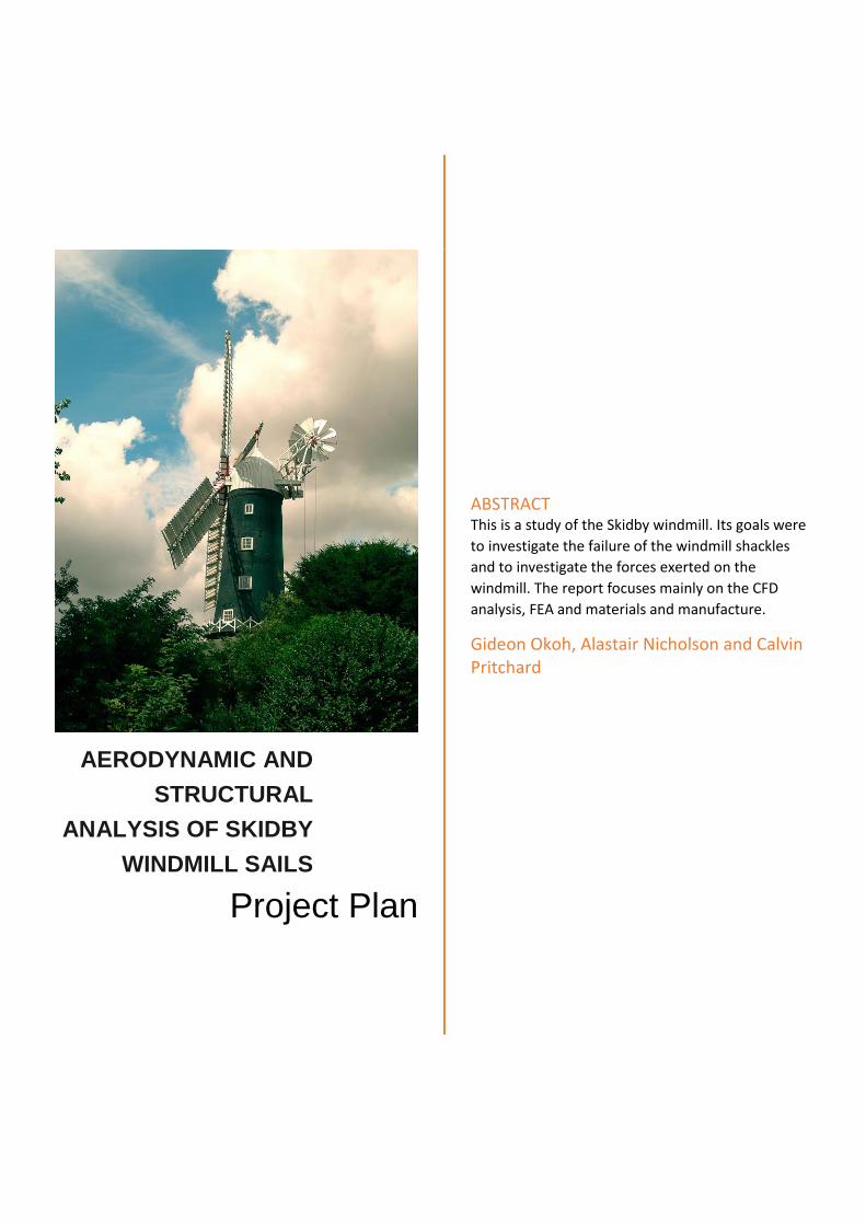
AERODYNAMIC AND STRUCTURAL ANALYSIS OF SKIDBY WINDMILL SAILS Project Plan ABSTRACT This is a study of the Skidby windmill. Its goals were to investigate the failure of the windmill shackles and to investigate the forces exerted on the windmill. The report focuses mainly on the CFD analysis, FEA and materials and manufacture. Gideon Okoh, Alastair Nicholson and Calvin Pritchard
-
Upload
gideon-okoh -
Category
Documents
-
view
80 -
download
4
Transcript of Skidby windmill Group Project Final
AERODYNAMIC AND
STRUCTURAL
ANALYSIS OF SKIDBY
WINDMILL SAILS
Project Plan
ABSTRACT This is a study of the Skidby windmill. Its goals were
to investigate the failure of the windmill shackles
and to investigate the forces exerted on the
windmill. The report focuses mainly on the CFD
analysis, FEA and materials and manufacture.
Gideon Okoh, Alastair Nicholson and Calvin Pritchard
1
Contents 1. Introduction ................................................................................................................................ 4
1.1 – Skidby Mill Background Information ...................................................................................... 4
1.2 – How the Skidby Mills Works................................................................................................... 5
1.3 – Project and Circumstantial Background ................................................................................. 7
1.4 – Aims and Objectives ............................................................................................................... 8
1.5 – Software Introduction and Validation.................................................................................... 8
1.6 – Gantt Chart ........................................................................................................................... 10
1.7 – Individual Goals and Objectives ........................................................................................... 12
2. Design Exercise – Calvin Pritchard ................................................................................................ 12
3. Materials and Manufacture – Gideon Okoh ................................................................................. 14
3.1 – Types of Material ................................................................................................................. 14
3.2 – Mechanical property of material ......................................................................................... 16
3.3 – Manufacturing ...................................................................................................................... 21
3.4 – Discussion ............................................................................................................................. 26
3.5 – Conclusion ............................................................................................................................ 26
4. CFD Analysis – Calvin Pritchard ..................................................................................................... 27
4.1 – Introduction to CFD of the Skidby Mill sails ......................................................................... 27
4.2 – Simple Sail ............................................................................................................................ 28
4.3 – Complex Sail ......................................................................................................................... 31
4.4 – Discussion ............................................................................................................................. 34
4.5 – Conclusion ............................................................................................................................ 35
5. FEA – Alastair Nicholson ............................................................................................................... 35
5.1 – Introduction ......................................................................................................................... 35
5.2 – Background .......................................................................................................................... 35
5.3 – Method ................................................................................................................................. 36
5.4 – Results .................................................................................................................................. 37
5.5 – Assumptions ......................................................................................................................... 41
5.6 – Limitations ............................................................................................................................ 42
5.7 – Discussion ............................................................................................................................. 42
5.8 – Conclusion ............................................................................................................................ 44
6. Power output – Gideon Okoh ....................................................................................................... 45
6.1 – Introduction ......................................................................................................................... 45
6.2 – Calculations .......................................................................................................................... 45
6.3 – Conclusion ............................................................................................................................ 49
7. Project management – Alastair Nicholson .................................................................................... 50
2
8. Final Discussion – Calvin Pritchard ................................................................................................ 51
9. Conclusion – Calvin Pritchard........................................................................................................ 52
10. Future work – Alastair Nicholson ................................................................................................ 53
11. References .................................................................................................................................. 53
12. Appendices .................................................................................................................................. 56
Figure 1 - Diagram of Skidby windmill (Skidby Mill Information Sheet, accessed 2014) .................... 5
Figure 2 - (Skidby Mill – How It Works, accessed 2014) ...................................................................... 7
Figure 3 ................................................................................................................................................... 7
Figure 4 - Picture of Skidby windmill shackles .................................................................................... 12
Figure 5 - Yield strength and thickness of a material (Kumar, n.d.) ..................................................... 17
Figure 6 - Graph of Yield strength of materials .................................................................................... 18
Figure 7 - Material strength vs toughness chart (NA, 2001) ................................................................. 19
Figure 8 - Ductile and brittle material behaviour (Anon., 2003) .......................................................... 20
Figure 9 - Typical S-N curve for medium strength Carbon Steel (Gandy, 2007 ) ................................ 21
Figure 10 - Forging at different temperatures (TYNE, 2013) ............................................................... 24
Figure 11 - Torch orientation and torch angle (defects, n.d.) ............................................................... 25
Figure 12 - Simple Sail ......................................................................................................................... 28
Figure 13 - Flow over simple sail ......................................................................................................... 30
Figure 14 - Flow over simple sail 2 ...................................................................................................... 30
Figure 15 - Complex Sail model ........................................................................................................... 31
Figure 16 - Flow over complex sail ...................................................................................................... 32
Figure 17 - Flow over complex sail 2 ................................................................................................... 32
Figure 18 - Pressure distribution on sails .............................................................................................. 34
Figure 19- Equivalent Stress contour plot of set up 1 ........................................................................... 38
Figure 20-Equivelent Stress contour plot for set up 1- vertical up ....................................................... 38
Figure 21-Equivelent Stress contour plot for set up 1- vertical down .................................................. 39
Figure 22-Equivalent Stress contour plot of set up 2 ............................................................................ 39
Figure 23-Equivalent Stress contour plot of set up 3 ............................................................................ 40
Figure 24- Total Deformation of shackles- set up 3 ............................................................................. 40
Figure 25- Life, Number of cycles to failure ........................................................................................ 41
Figure 26 - The (Cp) (above) and the torque coefficients (Ct) of various types of wind turbine rotor
plotted against tip-speed ratio (λ). (Fraenkel, 1986) ............................................................................. 46
Figure 27 - Swept area of a wind turbine (blog, 2010-2012) ................................................................ 47
Figure 28 - typical wind turbine power output with steady wind speed (Anon., n.d.) .......................... 49
Figure 29-Equivalent Stress contour plot of set up 3- Shackle 1 .......................................................... 57
Figure 30-Equivalent Stress contour plot of set up 3- Shackle 2 .......................................................... 57
Figure 31-Equivalent Stress contour plot of set up 3- Shackle 3 .......................................................... 58
Figure 32-Equivalent Stress contour plot of set up 3- Shackle 4 .......................................................... 58
Figure 33 - Concept Design 1 ............................................................................................................... 60
Figure 34 - Concept Design 2 ............................................................................................................... 60
Figure 35 - Concept Design 3 ............................................................................................................... 61
Figure 36 - Concept Design 4 ............................................................................................................... 61

3
Figure 37 - Concept Design 5 ............................................................................................................... 62
Table 1 - Project plan Gantt chart ......................................................................................................... 10
Table 2 - Yield strength and ultimate strength of the materials ............................................................ 17
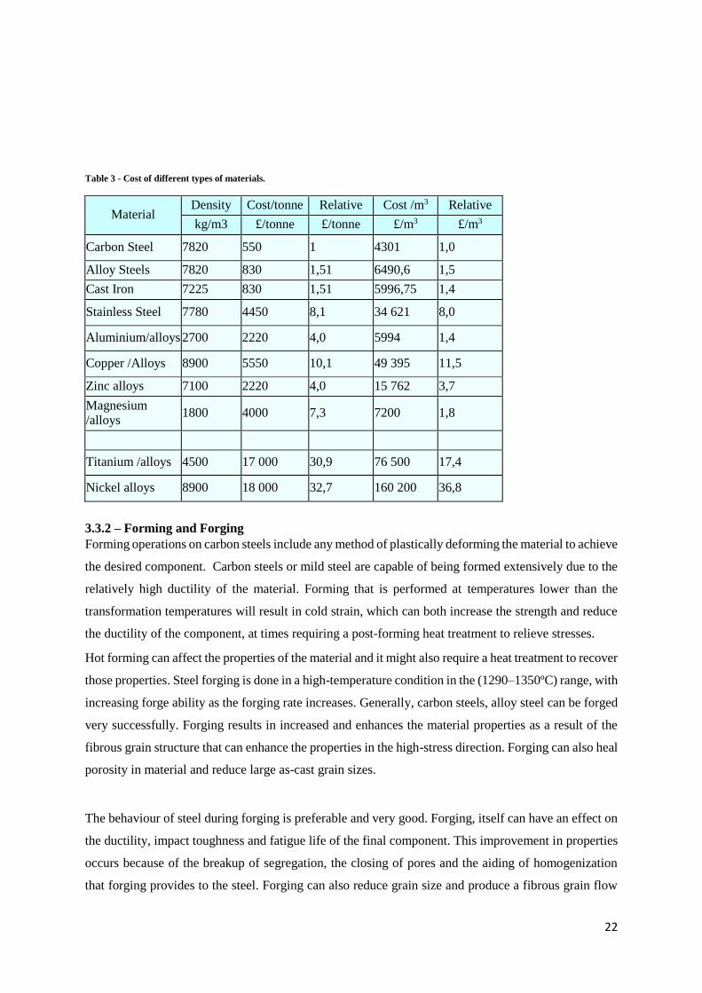
Table 3 - Cost of different types of materials. ...................................................................................... 22
Table 4 - Simple sail CFD data ............................................................................................................. 29
Table 5 - Complex sail CFD data.......................................................................................................... 31
Table 6 - Complex sail CFD data ............................................................................................................ 33
Table 7 - Maximum and Minimum Equivalent stress for set up 1 ........................................................ 38
Table 8 - Maximum and Minimum Equivalent stress for set up 2 ........................................................ 39
Table 9 - Maximum and Minimum Equivalent stress for set up 3 ........................................................ 40
Table 10 - Shows assumed the parameter of both wind turbine and windmill. .................................... 48
Table 11 - Maximum and Minimum Equivalent stress for set up 1- vertical up .................................. 56
Table 12 - Maximum and Minimum Equivalent stress for set up 1- vertical down ............................. 56
4
1. Introduction
1.1 – Skidby Mill Background Information
Windmills are machines that convert wind energy into rotational energy by means of sails or blades.
“Windmills are known to have been used to grind corn as far back as the seventh century but the
earliest recorded use is in AD915 in Seiston, a dry windy region on the borders of Iran and
Afghanistan”. (East Riding of Yorkshire Council 4, accessed 2014). There are originally designed to
mill grain for food production, such as the production of wholemeal flour, pumping water and sawing
wood etc. Windmills are grouped into vertical and horizontal mill, vertical mill consists of post mills,
smock mills and tower mills.
The focus of this project will be on tower mills, which is a ‘type of vertical windmill consisting of a
brick or stone tower, on which sits a wooden 'cap' or roof, which can rotate to bring the sails into the
wind.’ East Riding of Yorkshire Council say that the “Skidby Mill is a working four-sailed tower
windmill”, and that “the mill is unusual in still having all its original outbuildings around the
courtyard. Some of these have been converted to form the Museum of East Riding Rural Life” (East
Riding Museums & Galleries, accessed 2014). East Riding of Yorkshire Council 4 say (Accessed
2014) during the “18th century tower mills began to appear in East Yorkshire, although these had
originally been invented around three centuries earlier. In these only the top or cupola containing the
windshaft, sails and gearing, moves, the main body remains stationary”.
The first record of a mill on the present site appeared in 1764. This was a wooden post mill with two
pairs of stones. Skidby Mill was then built in 1821 by millwrights Norman and Smithson of Hull and
replaced an earlier post mill on the same site. But the Patent sails were invented in 1807, and are
designed to allow all the shutters to be opened and closed simultaneously while the sails are turning.
In 1854 the mill was owned by the Thompson’s family for over 100 years, who also owned a steam
roller mill in Hull and a water mill at Welton.
The Skidby Mill was originally used to produce animal foodstuffs, “In 1878 the mill was first
converted to the production of animal foodstuffs”. However, its use, or function, has varied greatly
over its lifespan. In 1954 the windmill changed from wind power to electrical power, with the main
tower of the mill converted to a grain silo, which would supply various animal feed machines. In 1962
Skidby Mill had to be sold to Allied Mills. Newer animal feed machines were brought in from the
Thompsons’ mill in Hull, and these can still be seen on the flour bagging floor.
5
In 1966 the mill ceased to operate commercially and was sold to Beverley Rural District Council, in
1974 the mill was restored to full working order re-utilising wind power after a 20 year gap. From
1974 to the present day, the windmill has been converted to the production of flour, milled from
English wheat in the traditional manner and is now owned and managed by the Museum of East
Riding Rural Life. “Skidby Windmill produces excellent quality, stone-ground, strong wholemeal
flour using traditional methods by our qualified miller and volunteers. The flour is suitable for bread
making, but it is versatile and can be used in cakes, biscuits, pastry and general baking. We have had
very good results from bread making machines too” (East riding of Yorkshire council 2, Accessed
2014).
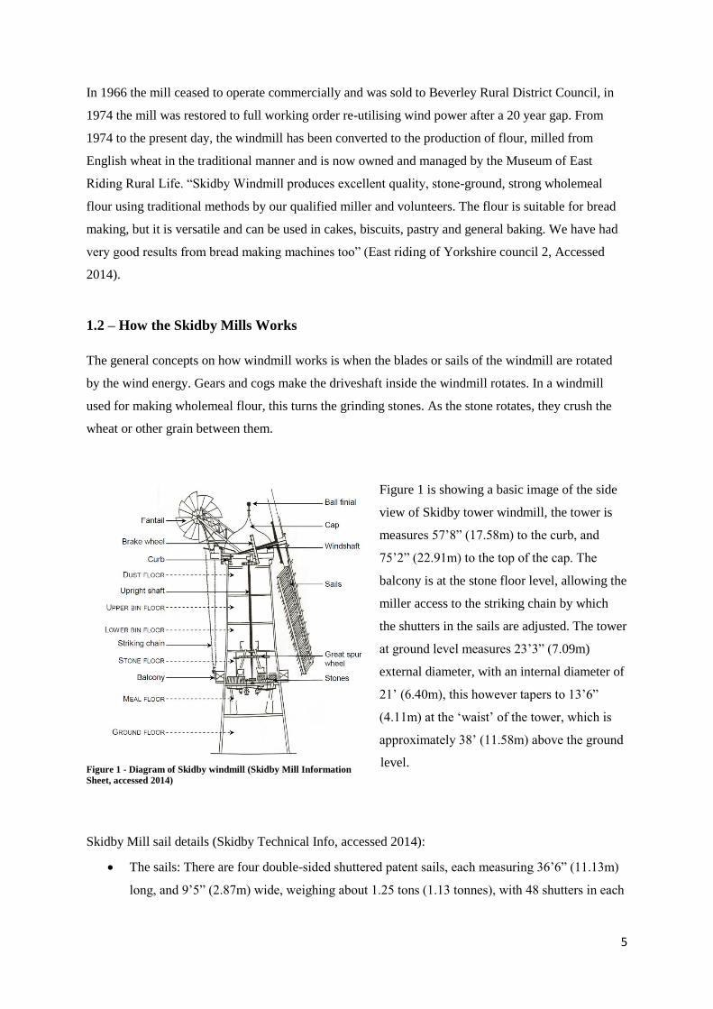
1.2 – How the Skidby Mills Works
The general concepts on how windmill works is when the blades or sails of the windmill are rotated
by the wind energy. Gears and cogs make the driveshaft inside the windmill rotates. In a windmill
used for making wholemeal flour, this turns the grinding stones. As the stone rotates, they crush the
wheat or other grain between them.
Figure 1 is showing a basic image of the side
view of Skidby tower windmill, the tower is
measures 57’8” (17.58m) to the curb, and
75’2” (22.91m) to the top of the cap. The
balcony is at the stone floor level, allowing the
miller access to the striking chain by which
the shutters in the sails are adjusted. The tower
at ground level measures 23’3” (7.09m)
external diameter, with an internal diameter of
21’ (6.40m), this however tapers to 13’6”
(4.11m) at the ‘waist’ of the tower, which is
approximately 38’ (11.58m) above the ground
level.
Skidby Mill sail details (Skidby Technical Info, accessed 2014):
The sails: There are four double-sided shuttered patent sails, each measuring 36’6” (11.13m)
long, and 9’5” (2.87m) wide, weighing about 1.25 tons (1.13 tonnes), with 48 shutters in each
Figure 1 - Diagram of Skidby windmill (Skidby Mill Information
Sheet, accessed 2014)
6
sail. The four sails have to be turned into the wind, this means the sails must always be facing
into the wind, otherwise this could damage to mill.
The shades: The leading side shades measure 40” (1.02m) by 12” (0.30m), whilst the
following shades measure 48” (1.22m) by 12” (0.30m).
Fantails: The Skidby’s fantail has 8 vanes on the rotor which is set at an angle to the wind, so
that when the wind changes direction the fantail starts to turn. It also have a bevelled gears
this turns the whole cap round on the curb at the top of the tower until the fantail stop
working, ensuring no damage is caused to the mill by off-direction wind.
Considering the different parts of the mill components on how the Skidby windmill mechanics works
by step by step process. First of all the four sails have to be turned into the wind, this means the sails
must always be facing into the wind. A wind from behind can seriously damage the sails and the cap.
The sails are turned into the wind by the fantail. If the sails are facing directly into the wind the fantail
doesn’t turn with the vanes of the fantail are set at an angle to the wind. If the wind changes direction
it catches the vanes, which start to turn. Fantail downshaft transfers the rotation of the fantail down to
the lower fan gear, and then it rotates the lower fan gear which transfers the rotation to the fantail spur
wheel. The fantail spur wheel is attached to the curb pinion by a horizontal shaft passing through the
outer shell of the cap. As the curb pinion rotates round the toothed curb, which runs right round the
top of the tower, it moves the whole cap and sails round the tower. Secondly the speed at which the
sails turn is governed by the shades: when the shades are open as here, the wind spills through and the
sails only turn slowly. Once the shades are set, an appropriate weight for the wind speed is hung on
the chain to keep the shades in the required position. In a gust of wind the shades are therefore able to
blow open and spill the wind through. As the striking rules move inwards they pull the arms on the
shades, which pivot closed. The third step is when the rotation of the sails is transferred to the stones,
the sails rotate, they turn the windshaft and the brake wheel vertically, “The wallower wheel is turned
by the brake wheel and transfers the rotation to the vertical drive shaft turns the great spur wheel,
which then turns the selected stones via the stone nut and the quant. The next step is followed by
grounding the grain. This is when the grain falls into the eye of the stone from the shoe”.(East riding
of Yorkshire Council, accessed 2014).
7
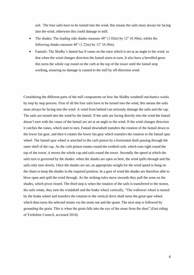
Figure 3
Figure 2 - (Skidby Mill – How It Works, accessed 2014)
Figure 2 shows a diagram of the Skidby Mill stone. As the upper stone rotates clockwise above the
stationary lower (bed) stone the furrows work in a scissor action, cutting the grain open and passing it
to the flat surfaces to be ground, then, the ground flour is worked outwards to the stone casing where it
falls out into the flour chute then down to the meal floor below to be bagged. The fifth step requires
getting the grain to the stone. This is done by tipping the grain is into the grain elevator bin at the base
of the tower. Inside the grain elevator they are a series of small buckets scoops the grain out of the bin
and carries it up to the bin floor, as the quant rotates, its square cross-section causes the shoe to shake.
This shaking causes the grain to drop into the eye of the stone at a rate appropriate to the speed of the
stone. Finally to stop the windmill the sails have to slow down as much as possible then the miller pulls
the brake rope, which hangs out of the cap near the striking chain. Once the mill has stopped, a wooden
block is pushed towards the brake wheel to prevent slippage.
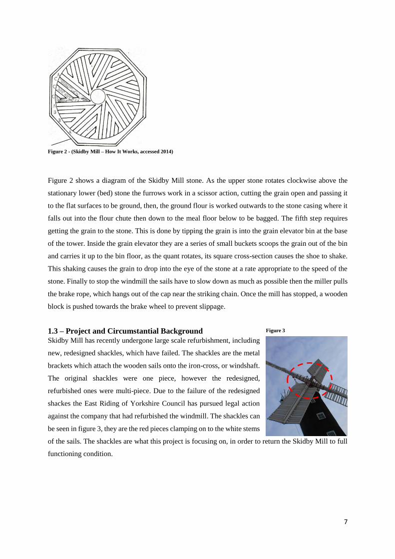
1.3 – Project and Circumstantial Background
Skidby Mill has recently undergone large scale refurbishment, including
new, redesigned shackles, which have failed. The shackles are the metal
brackets which attach the wooden sails onto the iron-cross, or windshaft.
The original shackles were one piece, however the redesigned,
refurbished ones were multi-piece. Due to the failure of the redesigned
shackes the East Riding of Yorkshire Council has pursued legal action
against the company that had refurbished the windmill. The shackles can
be seen in figure 3, they are the red pieces clamping on to the white stems
of the sails. The shackles are what this project is focusing on, in order to return the Skidby Mill to full
functioning condition.
8
1.4 – Aims and Objectives
This project aims to analyse and research into the causes of the failed shackles on the Skidby Windmill.
The analysis will uncover why the windmill’s shackles had failed, including the dissection of the
shackles’ design, material properties and manufacturing techniques. The loads exerted on the shackles
from the wind will need to be considered, thoroughly. Including the angle of the wooden sails, their
weight, and the ability to not only be able to function under maximum stress situations, but to be able
to withstand extreme weather situations also.
To, hopefully, acquire the failed shackles and examine the fracture surface, using metallography,
determining the cause of the failure in the shackles themselves and analysing their metallic structure.
Once the shackles, or brackets, have been conclusively analysed, a new, or even a refined design will
be digitally modelled and theoretically simulated. This remodelling will be an improvement on the
original, refurbished, shackles and should be much longer lasting theoretically. Cost, ease of
manufacturability, ease of installation, material choice and authenticity to the design of the windmill
will all be considered, as the windmill itself is Grade II* listed, and so there will be design limitations
associated with that.
To submit the design to East Riding of Yorkshire Council, for it to hopefully be manufactured and used
for the Skidby Mill.
The final aim is to theoretically calculate the power output of the Skidby Windmill, this would enable
the possibility to compare the, approximately, 200 year old technology to the power output from modern
day wind turbines.
1.5 – Software Introduction and Validation
The calculations and modelling for this project will largely be done on the computer, and a series of
applications will be used. Both 3D flow modelling and stress analysis are being considered in the project,
and the programs that will be used are SolidWorks for the flow modelling and ANSYS for the stress
analysis.
SolidWorks Flow Simulation is an inbuilt application in the SolidWorks suite, and will be used for its
Computational Fluid Dynamics, as it will allows you to “calculate fluid flow and heat transfer forces
and investigate the impactor a moving liquid or gas on product performance.” (2014, SolidWorks
Website). SolidWorks also does allow for Finite Element Analysis, however ANSYS will be used

9
instead. SolidWorks is a very widely used program, with nearly 2 million customers worldwide as of
2012, including over 165,000 companies (SolidWorks, 2012). SolidWorks provides accurate
simulations and dimensions and is fairly accurate in comparison to real world situations. Though for
this examination we cannot undertake in any real world testing in order to confirm whether or not the
results obtained are accurate and reliable or not. It will be assumed that the results gathered from
SolidWorks are reliable and accurate, due to the volume of users that rely on SolidWorks for their work.
Previous experience with SolidWorks has also been successful in terms of accuracy of its predictions.
ANSYS is an engineering specific program dedicated to meshing models and analysing the outcomes,
including stress and temperature calculations, amongst other measurement divisions. In a similar
situation to SolidWorks, it is not possible to examine whether or not the results that are obtained from
ANSYS are an accurate, reliable representation of the results that are obtained in the real world can’t
be obtained because the no real world tests will be undertaken.
10
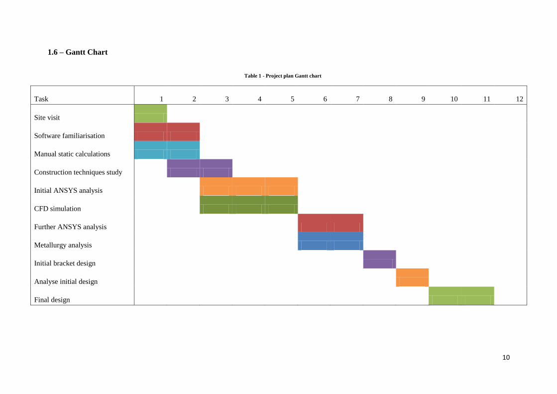
1.6 – Gantt Chart
Task 1 2 3 4 5 6 7 8 9 10 11 12
Site visit
Software familiarisation
Manual static calculations
Construction techniques study
Initial ANSYS analysis
CFD simulation
Further ANSYS analysis
Metallurgy analysis
Initial bracket design
Analyse initial design
Final design
Table 1 - Project plan Gantt chart
11
1.6.1 – Gantt Chart Tasks
Site Visit – Visit the site of the Skidby windmill to gain a better understanding of how it functions and
the exact function of the brackets.
Software Familiarisation – Familiarise ourselves with the ANSYS and SolidWorks software so that
we are confident with using the software. ANSYS is a finite element analysis software that can be used
to calculate stresses throughout a component. SolidWorks is a 3d CAD software that can be used to
model parts and can be used to run computational fluid dynamics or CFD simulations.
Manual static calculations – By hand, using a simplified model, calculate the forces acting upon the
windmill and the brackets. Use the results of this to give a general idea of the stresses involved before
using ANSYS.
Construction techniques study – Research the construction techniques used and determine if the
techniques used could have affected the brackets and determine if a better approach could have been
taken.
Initial ANSYS analysis – Using ANSYS calculate the stresses the bracket was under without
considering the wind. Use results to give an idea as to why the brackets might have failed.
CFD simulation – Using SolidWorks model the sails of the windmill and run CFD simulations on the
windmill to determine what forces the wind would exert on the brackets.
Further ANSYS analysis – Run further calculations on ANSYS taking into account the results of the
CFD simulations to determine if the wind had a big effect on the stresses within the brackets.
Metallurgy analysis – Examine the brackets and try to determine the type of failure that occurred. Look
at the fracture points and try to determine if the brackets failed because of creep or if they failed
suddenly.
Initial bracket design – Design an initial bracket that could be used as an alternative to the original,
using the data gathered from ANSYS and the CFD simulations.
Analyse initial design – Analyse the initial design to determine how effective and efficient the design
is. Use ANSYS to determine if the stresses will exceed the material properties.
Final Design – Make any changes that the analysis might have suggested.
12
1.7 – Individual Goals and Objectives
The tasks will be divided as evenly as possible with everyone contributing to each task. Everyone will
have some input on each task, however there will most likely be one individual taking the lead on a task.
The tasks will be completed like this as some of them will be too much work for an individual and it
will be more efficient to split the workload. At this point in the project it is difficult to outline exactly
what each member of the group will work on.
2. Design Exercise
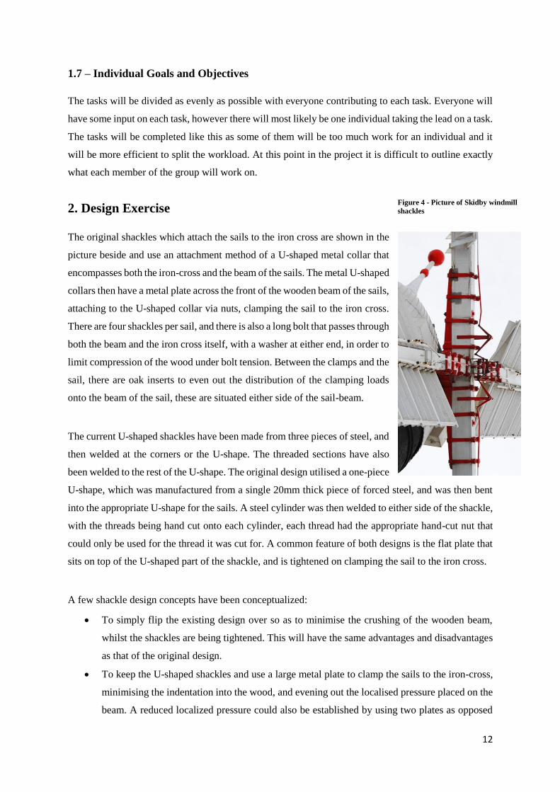
The original shackles which attach the sails to the iron cross are shown in the
picture beside and use an attachment method of a U-shaped metal collar that
encompasses both the iron-cross and the beam of the sails. The metal U-shaped
collars then have a metal plate across the front of the wooden beam of the sails,
attaching to the U-shaped collar via nuts, clamping the sail to the iron cross.
There are four shackles per sail, and there is also a long bolt that passes through
both the beam and the iron cross itself, with a washer at either end, in order to
limit compression of the wood under bolt tension. Between the clamps and the
sail, there are oak inserts to even out the distribution of the clamping loads
onto the beam of the sail, these are situated either side of the sail-beam.
The current U-shaped shackles have been made from three pieces of steel, and
then welded at the corners or the U-shape. The threaded sections have also
been welded to the rest of the U-shape. The original design utilised a one-piece
U-shape, which was manufactured from a single 20mm thick piece of forced steel, and was then bent
into the appropriate U-shape for the sails. A steel cylinder was then welded to either side of the shackle,
with the threads being hand cut onto each cylinder, each thread had the appropriate hand-cut nut that
could only be used for the thread it was cut for. A common feature of both designs is the flat plate that
sits on top of the U-shaped part of the shackle, and is tightened on clamping the sail to the iron cross.
A few shackle design concepts have been conceptualized:
To simply flip the existing design over so as to minimise the crushing of the wooden beam,
whilst the shackles are being tightened. This will have the same advantages and disadvantages
as that of the original design.
To keep the U-shaped shackles and use a large metal plate to clamp the sails to the iron-cross,
minimising the indentation into the wood, and evening out the localised pressure placed on the
beam. A reduced localized pressure could also be established by using two plates as opposed
Figure 4 - Picture of Skidby windmill
shackles
13
to one large plate, reducing weight as one approximately six foot long metal plate would be
heavy. This design can have many variations of the plate that bolts across the top of the beam.
The disadvantage associated with this is that the precision of the attachment holes for the U-
shaped shackles is much greater, as any imperfections in the wooden beam will affect the
clamping properties of this method. Also the increased weight of this design and the increased
cost of manufacturing are negatives. In order to reduce the weight effectively, extensive
machining would have to be done to the metal plate further increasing costs.
To use a long threaded bolt with two plates either side, this is very similar to the initial U-
shaped shackles. However, there will be a much smaller, and not flat, surface area in contact
with either side of the beam (if the beam is viewed from perpendicular to the iron cross). The
threads, could dig into the beam and under repeated loads, or general use, this could wear away
at the beam, reducing the lifespan of the beam. One way of reducing this issue is to have a
smooth central cylinder, and only have the threads on either end. Another issue with this design
is that a great deal of the tension is placed on the threads themselves, which are not of that a
great surface area. This would be a very cost conscious shackle system, and would also be a
very easy to repair system with very easily replaceable, attainable parts, and so this low cost
factor may offset the potentially shorter lifespan of the shackles.
To use a similar attachment method to that of repair of bone fractures, in that a large metal plate,
with splines protruding, is wrapped around the beam, the bent splines have a resistance to
springing back out, but also retain a little bit of flex. The disadvantages associated with this
method however are that it will be very difficult to install, a very heavy attachment method,
and more susceptible to fatigue, as well as being less secure than a bolted method, as well as
very difficult and expensive to manufacture.
Although not technically a different design concept, it could also be possible to propose that
more shackles are added to the sail, potentially distributing the load more evenly across a
greater number of shackles. This ‘concept’ can be proposed for any of the multiple shackle per
sail designs, allowing for the potential of more even distribution of forces over all the shackles.
An attachment method based on jubilee clips (or hose clips) could be used, in that a large band
of steel that comes back on itself with a bolt used to tighten the overlapping steel band. This
method of attachment would rely on the tensile properties of the steel in the band. In order to
have strength properties high enough, the steel will have to very thick, and could therefore
require the jubilee clip to be pre-bent to the shape characteristics of the sail and iron cross.
Advantages of this design would include a very even clamping force on the sail and iron cross,
as well as single bolt tightening ability. Jubilee clips are generally very useful where the item
being clamped is slightly compressible. Disadvantages include that it will be very awkward to
install the clamps, in that the sail would have to be slid through the jubilee clips and then
14
tightened on. Another disadvantage is that if the friction on the surfaces is too great, then the
evenness of the clamping will be compromised.
Though not a shackle design, altering the spacing characteristics of the shackles can result in
the same desired effects that a new shackle design would give. Namely reduced stresses on the
shackles, potentially resulting in a longer working life. If, for example, the stresses were found
to be greatest in the innermost shackle, and found to be the least in the outer most shackle, then
the spacing could be tailored appropriately, i.e. the inner two shackles are shifted more towards
the inner of the iron cross.
However, though these concepts have been proposed, for a listed windmill such as the Skidby Mill,
certain historic standards must be kept. It was therefore proposed by those who run the mill that the
shackle design is kept as close as possible to the original design. The more elaborate designs were
included due to their use in other areas of expertise.
3. Materials and Manufacture This section is based on the material that was used to manufacture the bracket (mild steel) and
investigating better alternate type of material such as the use of low alloy and stainless steel, titanium,
aluminium by focusing on the mechanical properties such as material yield strength, tensile strength,
elastic limit elastic/non-elastic behaviour, hardness, toughness, ductility and design life-durability of
the materials and comparing the properties of the materials. This section will also contain various
methods in which the materials could be manufactured into a possible and more durable bracket. Theses
method includes forging, casting, brazing and welding, and bending.
3.1 – Types of Material
3.1.1 – Mild steel
Mild steel, also known as low carbon steel, is currently the material used to manufacture the brackets.
Mild steel by definition, contains less carbon content than other steels and is inherently easier to cold-
form due to their soft and ductile nature. “Mild steel has low carbon content (up to 0.3%) and is therefore
neither extremely brittle nor ductile, it becomes malleable when heated, and so can be forged”.
(Wikipedia, 2010). Mild steels are good choices because they are easy to handle for example they are
easy to draw, bend, punch and also mild steels are the most common form of steel as its price is relatively
low while still providing reasonable material properties that are acceptable for many applications. It is
also often used where large amounts of steel need to be formed.
15
3.1.2 – Low alloy steel
Low alloy steel could be an alternative material that could have been used to manufacture the failed
brackets. This is because it can provide better mechanical properties than mild or carbon steels. Low-
alloy steels contain nickel, molybdenum, and chromium, which add to the material's weldability, notch
toughness, and yield strength. These alloys typically comprise 1 to 5 percent of the steel's content and
are added based on their ability to provide a very specific attribute. For example, “the addition of
molybdenum improves material strength; nickel adds toughness; and chromium increases temperature
strength, hardness, and corrosion resistance. Manganese and silicon, and other common alloying
elements, provide excellent deoxidizing capabilities”. (Packard, 2009).
But the most important alloy content that improve yield and ultimate strength and the general material
toughness are Mn, Ni, Cr, and Mo etc. “ combining molybdenum 0.15-0.25% with chromium, it
increases ultimate strength of steel without affecting ductility or workability”. (B, 2009) Low alloy
steel also contains very low carbon contents in order to produce adequate formability and weldability.
3.1.3 – Stainless steel
Another alternate material that could be used to manufacture the bracket is stainless steel. This is made
of iron alloys with a minimum of 10.5% chromium. Other alloying elements are added to enhance their
structure and properties such as formability, strength and toughness. These include metals such as:
nickel, molybdenum titanium and Copper etc. stainless steel is different from carbon steel by the amount
of chromium present. Unprotected carbon steel rusts readily when exposed to air and moisture in the
atmosphere. This is due to its anti-oxidation qualities, however stainless steel is often a popular solution
to corrosion related problems. Steel stainless would be the best replacement, if the mild steel bracket
had failed due to corrosive fatigue. Corrosive fatigue is the process where a material, due to corrosive
conditions and cyclic loads, experiences a mechanical degradation that leads to failure.
3.1.4 – Titanium
Thousands of titanium alloys have been developed and these can be grouped into four main categories.
Their properties depend on their basic chemical structure and the way they are manipulated during
manufacture. Some elements used for making alloys include aluminium, molybdenum, cobalt,
zirconium, tin, and vanadium. Alpha phase alloys have the lowest strength but are formable and
weldable. “Alpha plus beta alloys have high strength. Near alpha alloys have medium strength but have
good creep resistance. Beta phase alloys have the highest strength of any titanium alloys but they also
lack ductility.” (made, 2000)
16
Titanium is recognized physically and mechanically for its high strength to lightweight ratio. Titanium
metal is a strong metal with low density that is quite ductile, good workability and it is also highly
resistant to corrosive environment. Titanium metal is also twice as light and less dense than steel with
a density of 4.506 g·cm−3. “Titanium is as strong as some steels, but 45% less dense”. (2, 2007).
Titanium metals are selected for applications requiring high strength, low weight, high operating
temperature or high corrosion resistance which makes that’s while the use and applications of titanium
and its alloys are numerous. “The aerospace industry is the largest user of titanium products. It is useful
for this industry because of its high strength to weight ratio and high temperature properties”. (made,
2000).
3.1.5 – Aluminium
Pure aluminium is a silvery-white metal with many desirable characteristics. It is easily formed,
machined, and cast. Pure aluminium is soft compared to other metals and low strength, but alloys with
small amounts of copper, magnesium, silicon, manganese, and other elements have very useful
properties. “Aluminium is an abundant element in the earth's crust, but it is not found free in nature.
The Bayer process is used to refine aluminium from bauxite, an aluminium ore”. (WebElements, n.d.).
in terms of Strength to weight ratio, “Aluminium has a density around one third that of steel and is used
advantageously in applications where high strength and low weight are required. This includes vehicles
where low mass results in greater load capacity and reduced fuel consumption”. (Aalco, 2014).
Aluminium is corrosive resistant because when the surface of aluminium metal is exposed to air, a
protective oxide coating forms almost instantaneously. This oxide layer is corrosion resistant and can
be further enhanced with surface treatments such as anodising.
3.2 – Mechanical property of material
3.2.1 – Yield and ultimate strength of the materials
For metals the most common measure of strength is the yield strength, and the most important property
that the designer will need to use and observe before it is then used manufactured a product. Yield
strength of a material is the maximum stress that can be applied with a temporary deformation of the
test material or specimen. “Yield strength is usually defined at a specific amount of plastic strain, or
offset, which may vary by material and or specification”. (handbook, 2004 - 2006). While ultimate
17
tensile stress is the maximum stress value a specimen can undergo before it is fractured. In material
section, it is highly preferable to choose a material with higher yield strength. This is because higher
yield strength material can withstand a higher load applied to the material whilst being undamaged and
remain in un-deformed state afterwards. “More recently, structures have been designed using plastic
design concepts whereby the ability of the structure to yield and redistribute load without catastrophic
failure is required. In such cases the post-yield behaviour” (Trail, 1996)
The thickness can also affect the yield strength of a material for example increasing the thickness of a
plate or a section can reduce the yield strength of a material and the machinability, this is shown on
figure 5.
Figure 5 - Yield strength and thickness of a material (Kumar, n.d.)
Table 2 - Yield strength and ultimate strength of the materials
Material Average yield strength( MPa) UTS (MPa)
Mild steel 280 450
Low alloy steel 690 760
Stainless steel-cold rolled 520 860
Titanium 880 950
Aluminium 97 186
18
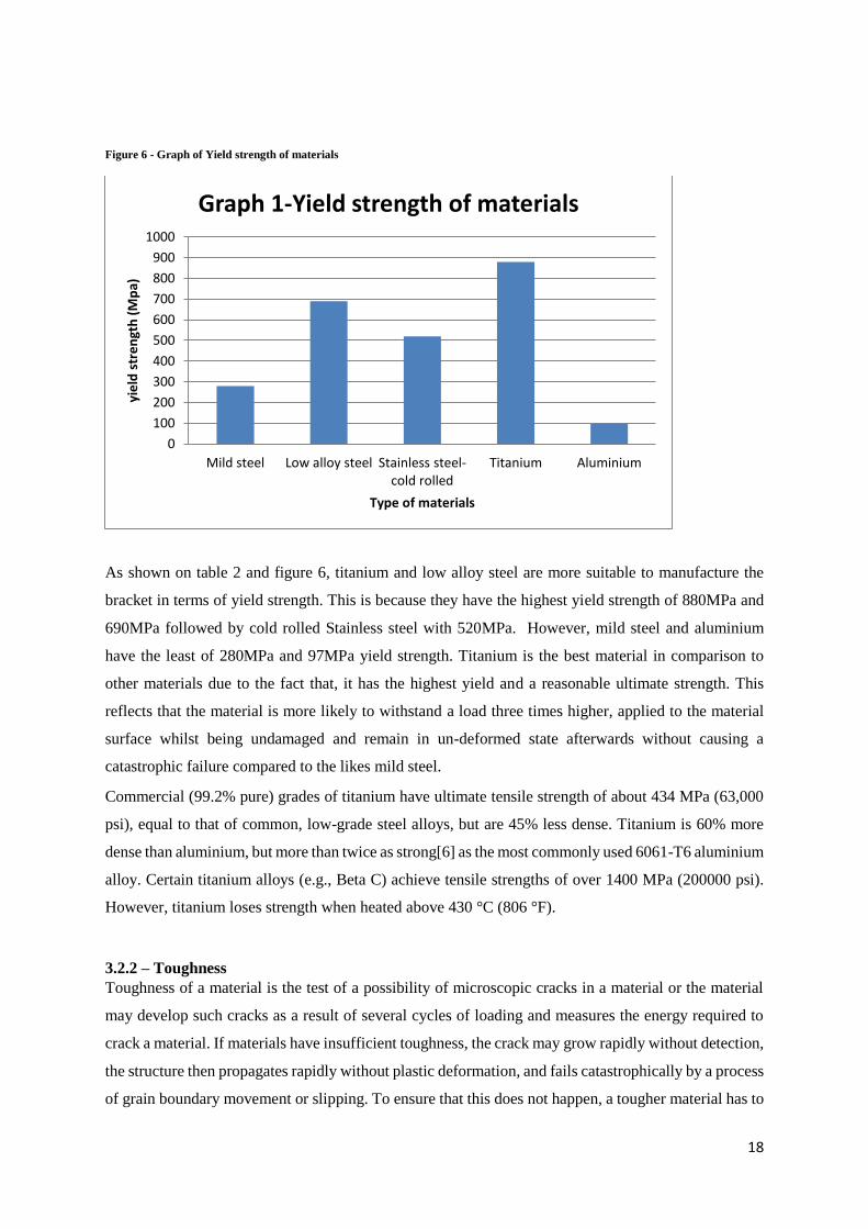
Figure 6 - Graph of Yield strength of materials
As shown on table 2 and figure 6, titanium and low alloy steel are more suitable to manufacture the
bracket in terms of yield strength. This is because they have the highest yield strength of 880MPa and
690MPa followed by cold rolled Stainless steel with 520MPa. However, mild steel and aluminium
have the least of 280MPa and 97MPa yield strength. Titanium is the best material in comparison to
other materials due to the fact that, it has the highest yield and a reasonable ultimate strength. This
reflects that the material is more likely to withstand a load three times higher, applied to the material
surface whilst being undamaged and remain in un-deformed state afterwards without causing a
catastrophic failure compared to the likes mild steel.
Commercial (99.2% pure) grades of titanium have ultimate tensile strength of about 434 MPa (63,000
psi), equal to that of common, low-grade steel alloys, but are 45% less dense. Titanium is 60% more
dense than aluminium, but more than twice as strong[6] as the most commonly used 6061-T6 aluminium
alloy. Certain titanium alloys (e.g., Beta C) achieve tensile strengths of over 1400 MPa (200000 psi).
However, titanium loses strength when heated above 430 °C (806 °F).
3.2.2 – Toughness
Toughness of a material is the test of a possibility of microscopic cracks in a material or the material
may develop such cracks as a result of several cycles of loading and measures the energy required to
crack a material. If materials have insufficient toughness, the crack may grow rapidly without detection,
the structure then propagates rapidly without plastic deformation, and fails catastrophically by a process
of grain boundary movement or slipping. To ensure that this does not happen, a tougher material has to
Mild steel Low alloy steel Stainless steel-cold rolled
Titanium Aluminium
0
100
200
300
400
500
600
700
800
900
1000
Type of materials
yie
ld s
tre
ngt
h (
Mp
a)
Graph 1-Yield strength of materials
19
be used, and in this case the cracks growth propagates slowly. During the cold winter, metal becomes
more vulnerable to failure by propagation of cracks. This is due to the toughness of the steel, and its
ability to resist this behaviour, decreasing as the temperature decreases. In addition, the toughness
required, at any given temperature, increases with the thickness of the material and increasing strength
usually leads to decreased toughness.
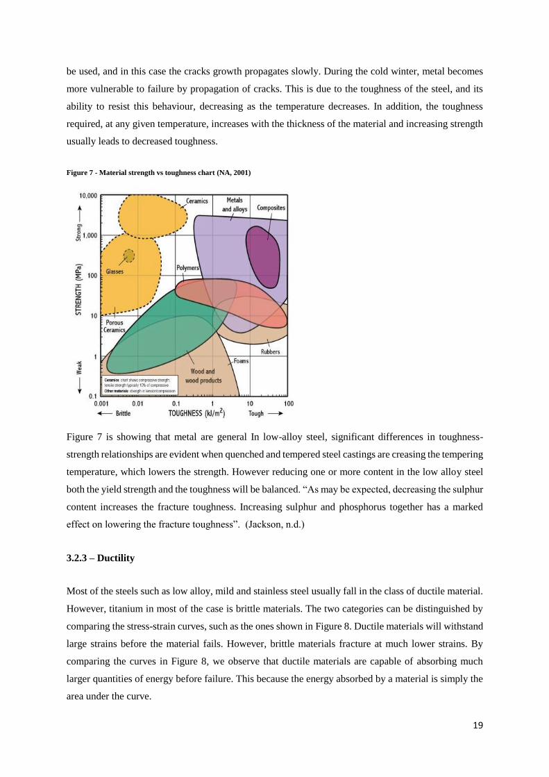
Figure 7 - Material strength vs toughness chart (NA, 2001)
Figure 7 is showing that metal are general In low-alloy steel, significant differences in toughness-
strength relationships are evident when quenched and tempered steel castings are creasing the tempering
temperature, which lowers the strength. However reducing one or more content in the low alloy steel
both the yield strength and the toughness will be balanced. “As may be expected, decreasing the sulphur
content increases the fracture toughness. Increasing sulphur and phosphorus together has a marked
effect on lowering the fracture toughness”. (Jackson, n.d.)
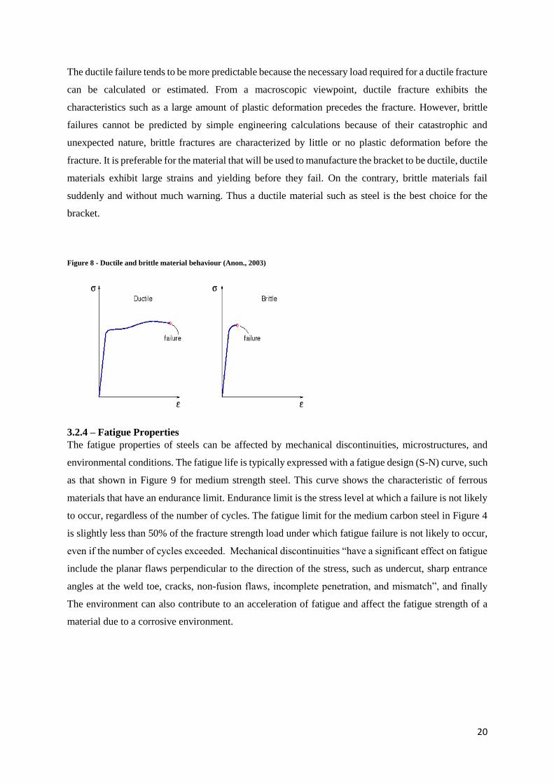
3.2.3 – Ductility
Most of the steels such as low alloy, mild and stainless steel usually fall in the class of ductile material.
However, titanium in most of the case is brittle materials. The two categories can be distinguished by
comparing the stress-strain curves, such as the ones shown in Figure 8. Ductile materials will withstand
large strains before the material fails. However, brittle materials fracture at much lower strains. By
comparing the curves in Figure 8, we observe that ductile materials are capable of absorbing much
larger quantities of energy before failure. This because the energy absorbed by a material is simply the
area under the curve.
20
The ductile failure tends to be more predictable because the necessary load required for a ductile fracture
can be calculated or estimated. From a macroscopic viewpoint, ductile fracture exhibits the
characteristics such as a large amount of plastic deformation precedes the fracture. However, brittle
failures cannot be predicted by simple engineering calculations because of their catastrophic and
unexpected nature, brittle fractures are characterized by little or no plastic deformation before the
fracture. It is preferable for the material that will be used to manufacture the bracket to be ductile, ductile
materials exhibit large strains and yielding before they fail. On the contrary, brittle materials fail
suddenly and without much warning. Thus a ductile material such as steel is the best choice for the
bracket.
Figure 8 - Ductile and brittle material behaviour (Anon., 2003)
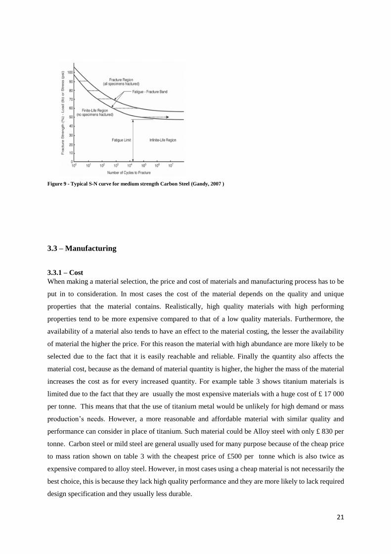
3.2.4 – Fatigue Properties
The fatigue properties of steels can be affected by mechanical discontinuities, microstructures, and
environmental conditions. The fatigue life is typically expressed with a fatigue design (S-N) curve, such
as that shown in Figure 9 for medium strength steel. This curve shows the characteristic of ferrous
materials that have an endurance limit. Endurance limit is the stress level at which a failure is not likely
to occur, regardless of the number of cycles. The fatigue limit for the medium carbon steel in Figure 4
is slightly less than 50% of the fracture strength load under which fatigue failure is not likely to occur,
even if the number of cycles exceeded. Mechanical discontinuities “have a significant effect on fatigue
include the planar flaws perpendicular to the direction of the stress, such as undercut, sharp entrance
angles at the weld toe, cracks, non-fusion flaws, incomplete penetration, and mismatch”, and finally
The environment can also contribute to an acceleration of fatigue and affect the fatigue strength of a
material due to a corrosive environment.
21
Figure 9 - Typical S-N curve for medium strength Carbon Steel (Gandy, 2007 )
3.3 – Manufacturing
3.3.1 – Cost
When making a material selection, the price and cost of materials and manufacturing process has to be
put in to consideration. In most cases the cost of the material depends on the quality and unique
properties that the material contains. Realistically, high quality materials with high performing
properties tend to be more expensive compared to that of a low quality materials. Furthermore, the
availability of a material also tends to have an effect to the material costing, the lesser the availability
of material the higher the price. For this reason the material with high abundance are more likely to be
selected due to the fact that it is easily reachable and reliable. Finally the quantity also affects the
material cost, because as the demand of material quantity is higher, the higher the mass of the material
increases the cost as for every increased quantity. For example table 3 shows titanium materials is
limited due to the fact that they are usually the most expensive materials with a huge cost of £ 17 000
per tonne. This means that that the use of titanium metal would be unlikely for high demand or mass
production’s needs. However, a more reasonable and affordable material with similar quality and
performance can consider in place of titanium. Such material could be Alloy steel with only £ 830 per
tonne. Carbon steel or mild steel are general usually used for many purpose because of the cheap price
to mass ration shown on table 3 with the cheapest price of £500 per tonne which is also twice as
expensive compared to alloy steel. However, in most cases using a cheap material is not necessarily the
best choice, this is because they lack high quality performance and they are more likely to lack required
design specification and they usually less durable.
22
Table 3 - Cost of different types of materials.
Material Density Cost/tonne Relative Cost /m3 Relative
kg/m3 £/tonne £/tonne £/m3 £/m3
Carbon Steel 7820 550 1 4301 1,0
Alloy Steels 7820 830 1,51 6490,6 1,5
Cast Iron 7225 830 1,51 5996,75 1,4
Stainless Steel 7780 4450 8,1 34 621 8,0
Aluminium/alloys 2700 2220 4,0 5994 1,4
Copper /Alloys 8900 5550 10,1 49 395 11,5
Zinc alloys 7100 2220 4,0 15 762 3,7
Magnesium /alloys
1800 4000 7,3 7200 1,8
Titanium /alloys 4500 17 000 30,9 76 500 17,4
Nickel alloys 8900 18 000 32,7 160 200 36,8
3.3.2 – Forming and Forging
Forming operations on carbon steels include any method of plastically deforming the material to achieve
the desired component. Carbon steels or mild steel are capable of being formed extensively due to the
relatively high ductility of the material. Forming that is performed at temperatures lower than the
transformation temperatures will result in cold strain, which can both increase the strength and reduce
the ductility of the component, at times requiring a post-forming heat treatment to relieve stresses.
Hot forming can affect the properties of the material and it might also require a heat treatment to recover
those properties. Steel forging is done in a high-temperature condition in the (1290–1350ºC) range, with
increasing forge ability as the forging rate increases. Generally, carbon steels, alloy steel can be forged
very successfully. Forging results in increased and enhances the material properties as a result of the
fibrous grain structure that can enhance the properties in the high-stress direction. Forging can also heal
porosity in material and reduce large as-cast grain sizes.
The behaviour of steel during forging is preferable and very good. Forging, itself can have an effect on
the ductility, impact toughness and fatigue life of the final component. This improvement in properties
occurs because of the breakup of segregation, the closing of pores and the aiding of homogenization
that forging provides to the steel. Forging can also reduce grain size and produce a fibrous grain flow
23
in the component. If the grain flow is oriented perpendicular to the crack that would be generated during
use (due to either impact or fatigue loading), the grain flow can hinder the propagation of the crack and
improve the forging’s impact and fatigue properties. While forged steel generally has superior fatigue
and toughness properties which most of the material with high quality performing material should
contain. However, forging has only small or minor effect on the final hardness and strength of the
component. Hardness and strength are normally controlled by the steel composition selected and the
heat treatments. There are different temperatures materials can be forged at:
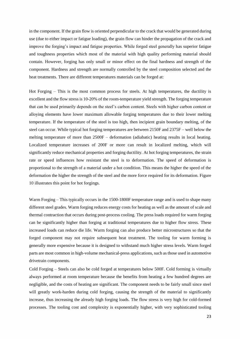
Hot Forging – This is the most common process for steels. At high temperatures, the ductility is
excellent and the flow stress is 10-20% of the room-temperature yield strength. The forging temperature
that can be used primarily depends on the steel’s carbon content. Steels with higher carbon content or
alloying elements have lower maximum allowable forging temperatures due to their lower melting
temperature. If the temperature of the steel is too high, then incipient grain boundary melting, of the
steel can occur. While typical hot forging temperatures are between 2150F and 2375F – well below the
melting temperature of more than 2500F – deformation (adiabatic) heating results in local heating.
Localized temperature increases of 200F or more can result in localized melting, which will
significantly reduce mechanical properties and forging ductility. At hot forging temperatures, the strain
rate or speed influences how resistant the steel is to deformation. The speed of deformation is
proportional to the strength of a material under a hot condition. This means the higher the speed of the
deformation the higher the strength of the steel and the more force required for its deformation. Figure
10 illustrates this point for hot forgings.
Warm Forging – This typically occurs in the 1500-1800F temperature range and is used to shape many
different steel grades. Warm forging reduces energy costs for heating as well as the amount of scale and
thermal contraction that occurs during post-process cooling. The press loads required for warm forging
can be significantly higher than forging at traditional temperatures due to higher flow stress. These
increased loads can reduce die life. Warm forging can also produce better microstructures so that the
forged component may not require subsequent heat treatment. The tooling for warm forming is
generally more expensive because it is designed to withstand much higher stress levels. Warm forged
parts are most common in high-volume mechanical-press applications, such as those used in automotive
drivetrain components.
Cold Forging – Steels can also be cold forged at temperatures below 500F. Cold forming is virtually
always performed at room temperature because the benefits from heating a few hundred degrees are
negligible, and the costs of heating are significant. The component needs to be fairly small since steel
will greatly work-harden during cold forging, causing the strength of the material to significantly
increase, thus increasing the already high forging loads. The flow stress is very high for cold-formed
processes. The tooling cost and complexity is exponentially higher, with very sophisticated tooling
24
assemblies required to absorb contact pressures well in excess of 100,000 psi. Cold-formed parts are
limited to coining operations and high-volume mechanical-press applications such as fasteners, spark-
plug bodies, bearing components and hand tools.
Figure 10 - Forging at different temperatures (TYNE, 2013)
3.3.3 – Weldability and welding method.
The main objective in wielding is to produce a continuous and homogeneous component with minimum
disruption of a parent microstructure. Weldability is defined as the capacity of a material to be welded
under the imposed fabrication conditions into a specific, suitably designed structure and to perform
satisfactorily in the intended service. Carbon steel is generally considered to be quite weldable,
particularly when the carbon content is below 0.35%, which it is by specification in all of the materials
covered in this report. A wide variety of processes are available to weld carbon steel satisfactorily, with
properties and composition comparable in the weld and the base material. The term weldability is also
used in a narrower sense to mean the ease with which a material can be welded without cracking or
other discontinuities. It is this meaning that is more relevant to the welding qualification.
To ensure your welding success, filler metals for low-alloy steels should match or exceed the base
metals tensile and yield strengths, as well as its elongation and toughness (Charpy V-notch) properties.
A perfect match is not always possible, however, so it is necessary to find the closest one possible.
When welding these low-alloys steels, preheat and post-heat treatments typically are not required.
Always refer to the welding procedure to determine the requirements.
The wide ranges of ultimate tensile strength, yield strength, and hardness are largely different due to
different heat treatment conditions. However welding defect that may occur during or after the process
can reduce the service performance of welded components. Such defects are gas porosity, hot tearing,
25
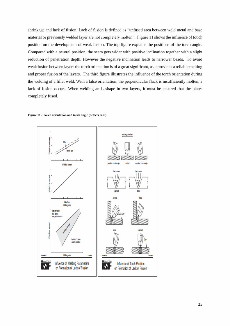
shrinkage and lack of fusion. Lack of fusion is defined as “unfused area between weld metal and base
material or previously welded layer are not completely molten”. Figure 11 shows the influence of touch
position on the development of weak fusion. The top figure explains the positions of the torch angle.
Compared with a neutral position, the seam gets wider with positive inclination together with a slight
reduction of penetration depth. However the negative inclination leads to narrower beads. To avoid
weak fusion between layers the torch orientation is of a great significant, as it provides a reliable melting
and proper fusion of the layers. The third figure illustrates the influence of the torch orientation during
the welding of a fillet weld. With a false orientation, the perpendicular flack is insufficiently molten, a
lack of fusion occurs. When welding an L shape in two layers, it must be ensured that the plates
completely fused.
Figure 11 - Torch orientation and torch angle (defects, n.d.)
26
3.4 – Discussion
The shackles for the Skidby Mill need to be strong, have good fatigue resistance, and be usable in British
weather conditions, whilst being cost effective. Weight is not of concern in these circumstances, and
strength is the main priority, with reparability being an important factor as well. The original shackles
were made from forged steel, and though not indestructible, did last for a long period of time (≈50
years), however during this time the shackles had to be repaired by re-welding, particularly of the
corners of the U-shape, which was a fairly frequent occurrence, in that it was done every few years, due
to the fatigues associated with the repetitive loading and unloading and opposite direction loading
associated with the shackles on a windmill. The ‘old fashioned’ way in which the shackles were
improved was simply to make them ‘bigger’, be that thicker, or wider, just generally making the
components larger.
Aluminium shackles would have to be really quite large in order to have a similar strength to a steel
component, not complying with the historical ‘look’ that the Skidby mill needs to adhere to. Aluminium
also reaches its endurance limit quicker than even mild steel, hence with lifespan of the shackles being
a high priority, aluminium is not the most suited to the task. Titanium on the other hand has all the
desired characteristics the metal for the shackles should have, namely, strength, ease of being put into
shape, correct size for aesthetics and excellent fatigue resistance at the temperatures at which the mill
operates, and a high corrosion resistance. However titanium is not a cheap material, it is also quite
difficult to obtain, much more so than, for example, steel. Titanium is also difficult to repair, or weld
as specialist tools are required due to the high temperatures, this lack of reparability along with the fact
that it was the most expensive metal considered renders it as a ‘money no object’ option, though in the
real world a more cost effective solution is needed.
This then leaves a form of steel to be used for the shackles, mild steel does not have strength
characteristics that are realistically high enough to be used, however both alloy steel and stainless steel
do. Stainless steel has very desirable corrosion resistance abilities in comparison to the alloy steel,
however it costs approximately five times the price of alloy steel making it a less tempting option.
Though the corrosion properties of the alloy steel are less than ideal, a protective coating, in the form
of paint could be applied for a small cost, negating, somewhat, the advantage of stainless steel.
3.5 – Conclusion
Alloy steel is the ideal material for the shackles to be made from, its strength, ability to be shaped and
welded, and fatigue characteristics at a reasonable price make it the ideal metal for the shackles to be
27
made from. If the temperatures at which the shackles had to operate in were different, then steel might
be less suited, the only factor that doesn’t work to alloy steel’s favour is its oxidising properties. The
East Yorkshire weather does include rain, and occasionally even snow, this moisture, when combined
with oxygen contained in the air can lead to the corrosion of unprotected alloy steel. Therefore the
shackle should be painted, to both protect the steel, and to match aesthetically with the rest of the mill.
4. CFD Analysis
4.1 – Introduction to CFD of the Skidby Mill sails
CFD, or computational fluid dynamics is a type of fluid mechanics which utilises algorithms and
numerical calculations to solve problems to do with fluid flow. The calculations are completed by
computers, simulating the interaction of liquids and gases with the model that has been simulated. CFD
software can be used to simulate very complex scenarios, including turbulent airflow, and even very
high, supersonic velocities. The basis of nearly all CFD problems are the Navier-Stokes equations.
Though CFD simulations can be incredibly accurate, and give great insight into how something behaves
under the inputted fluid loads, it is crucial that real world full scale testing is undertaken as well before
a product is put to market. CFD analysis is only effective if the inputs are correctly identified and chosen,
for example the type of fluid, the speed at which the fluid is ‘hitting’ the model, and where it comes
into contact with the model. These inputs are vital to the accuracy of the simulation, and so the results
are dependent on the appropriate values being inputted.
The CFD analysis was done on two, to scale models of the actual sails from Skidby Mill, one being a
plain flat sail surface, signifying the most simple, ‘basic’ shape that the sail can take. Whilst the other
being a near exact digital replica with the shades being in place to the dimensions obtained from the
windmill during refurbishment. The beam is assumed to be tapering consistently, with the angle at
which it tapers being taken from the dimensions located around the shackles. The shades of the
‘complex’ model are in the fully closed position, as this position provides the most possible drive for
the windmill, and the most possible resistance to the wind. Hence with the shades in this position, the
greatest forces can be simulated against the sail, therefore transmitting the highest loads and stresses to
the shackles on the iron-cross. The sails were chosen to be closed to simulate a ‘worst possible scenario’
situation for the loads on the shackles. The only thing that was not taken into account is that there is a
slight twist towards the tip of the following shades of each of the sails, this twist was not recreated as it
was not possible to measure the twist of the sail.
28
The chosen wind-speed for the simulations was 25m/s (≈ 49 knots). This speed was chosen as it
represents a stormy conditions with a very strong wind, or even strong gusting wind that is of a much
greater speed than what the mill operates at. The maximum wind-speed at which the mill operates is 25
knots (≈ 13m/s), as wind-speeds greater than this cause difficulties to stop the windmill. So by
simulating roughly the twice the wind-speed as what will be experienced by the sails when operating,
it will be ensured that the shackles will be able to withstand operating wind-speeds. However, it should
be noted that in storm situations, where the windmill is stopped, the sails may have to experience the
static loads from wind speeds as high as 25m/s, though the rotating forces will not have to be taken into
account. In extreme situations, the wind-speeds can exceed 70mph (≈ 31m/s or ≈ 61 knots) in the East
Yorkshire area, however winds of this speed are bordering on hurricane force, and widespread
destruction would occur, it is likely that other windmill components would be damaged also, not just
the shackles, and so it would be unnecessary to simulate these very rare situations due to both their
unlikeliness, and the fact that other damage will occur to other vital components of the mill.
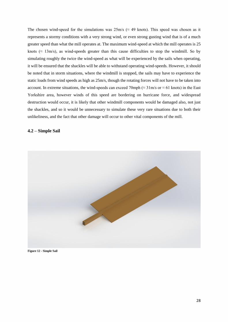
4.2 – Simple Sail
Figure 12 - Simple Sail
29
Table 4 - Simple sail CFD data
Goal Name Unit Value
Averaged
Value
Minimum
Value
Maximum
Value Delta Criteria
SG Min Static
Pressure
[Pa] 100662.8269 100661.8725 100657.9441 100664.8146 6.870473943 275.930871
SG Av Static
Pressure
[Pa] 101373.1343 101371.1264 101369.0404 101373.1661 3.744712339 11.2187038
SG Max Static
Pressure
[Pa] 101776.1555 101775.8025 101774.9958 101776.5768 1.580944043 541.1206608
SG Bulk Av
Static Pressure
[Pa] 101373.1343 101371.1264 101369.0404 101373.1661 3.744712339 11.2187038
SG Min Total
Pressure
[Pa] 100662.8269 100661.8725 100657.9441 100664.8146 6.870473943 275.930871
SG Av Total
Pressure
[Pa] 101373.1343 101371.1264 101369.0404 101373.1661 3.744712339 11.2187038
SG Max Total
Pressure
[Pa] 101776.1555 101775.8025 101774.9958 101776.5768 1.580944043 541.1206608
SG Bulk Av
Total Pressure
[Pa] 101373.1343 101371.1264 101369.0404 101373.1661 3.744712339 11.2187038
SG Normal
Force [N] 14590.31737 14610.74906 14531.40633 14724.65541 111.8545635 618.0600871
SG Normal
Force (X) [N] 3375.677019 3372.188783 3325.530874 3428.029785 30.1440989 177.7203835
SG Normal
Force (Y) [N] 14194.43968 14216.25246 14145.7614 14320.05702 107.890388 592.4470733
SG Normal
Force (Z) [N] -6.896468103 -7.134732609 -7.568348444 -6.895289437 0.544559313 2.974319705
SG Force [N] 14591.71226 14612.18182 14532.86996 14726.0795 111.8625872 618.1990893
SG Force (X) [N] 3369.510758 3365.782122 3317.955042 3422.831733 30.0781339 177.5520022
SG Force (Y) [N] 14197.33903 14219.24239 14149.04429 14322.76528 107.9203816 592.6478707
SG Force (Z) [N] -5.326688158 -5.562892954 -6.042862392 -5.317751563 0.553430179 3.034949453
The data obtained for the simple model of the sail is surprising in that both normal and regular forces
for the Z-axis are negative values. This therefore implies that the sail is being pulled away from the iron
cross due to the wind acting on it, which is unexpected result. The air pressure on the sail is on average
approximately 45Pa higher than that of atmospheric pressure.
30
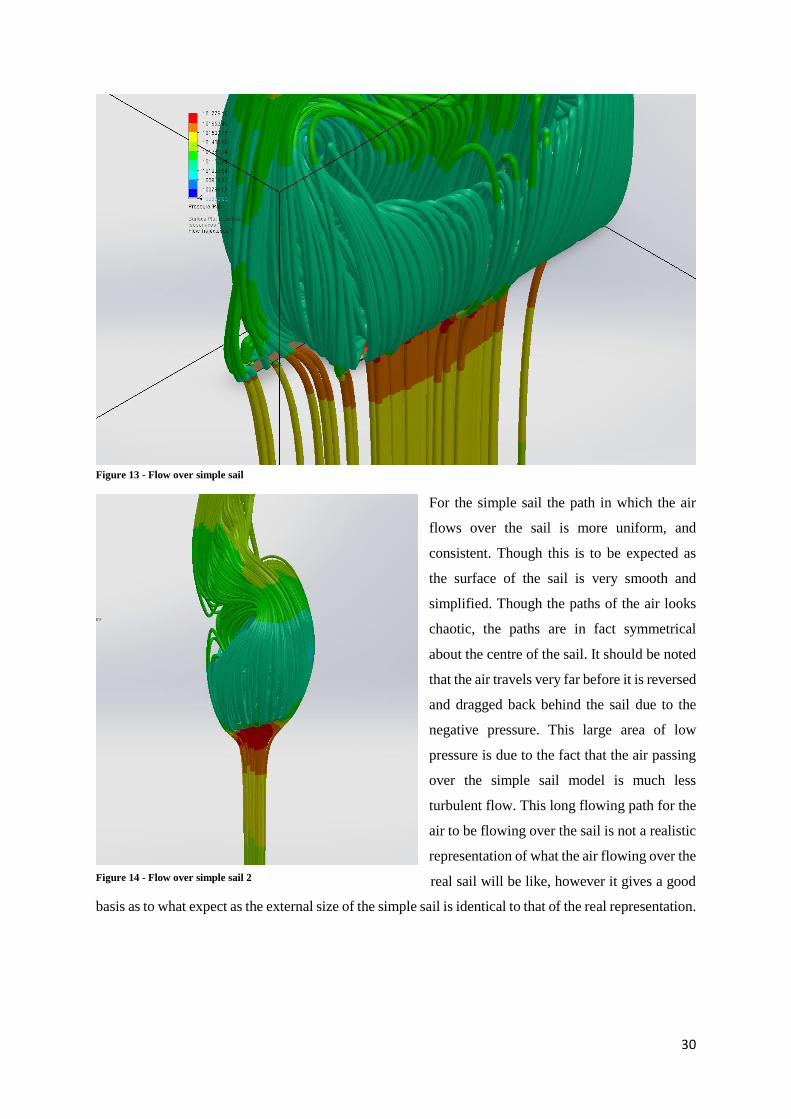
Figure 13 - Flow over simple sail
For the simple sail the path in which the air
flows over the sail is more uniform, and
consistent. Though this is to be expected as
the surface of the sail is very smooth and
simplified. Though the paths of the air looks
chaotic, the paths are in fact symmetrical
about the centre of the sail. It should be noted
that the air travels very far before it is reversed
and dragged back behind the sail due to the
negative pressure. This large area of low
pressure is due to the fact that the air passing
over the simple sail model is much less
turbulent flow. This long flowing path for the
air to be flowing over the sail is not a realistic
representation of what the air flowing over the
real sail will be like, however it gives a good
basis as to what expect as the external size of the simple sail is identical to that of the real representation.
Figure 14 - Flow over simple sail 2
31
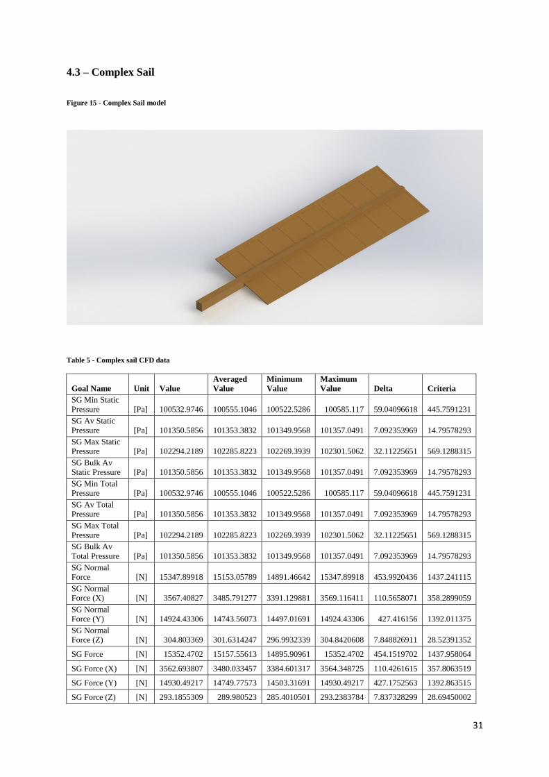
4.3 – Complex Sail
Figure 15 - Complex Sail model
Table 5 - Complex sail CFD data
Goal Name Unit Value
Averaged
Value
Minimum
Value
Maximum
Value Delta Criteria
SG Min Static
Pressure
[Pa] 100532.9746 100555.1046 100522.5286 100585.117 59.04096618 445.7591231
SG Av Static Pressure
[Pa] 101350.5856 101353.3832 101349.9568 101357.0491 7.092353969 14.79578293
SG Max Static Pressure
[Pa] 102294.2189 102285.8223 102269.3939 102301.5062 32.11225651 569.1288315
SG Bulk Av Static Pressure
[Pa] 101350.5856 101353.3832 101349.9568 101357.0491 7.092353969 14.79578293
SG Min Total Pressure
[Pa] 100532.9746 100555.1046 100522.5286 100585.117 59.04096618 445.7591231
SG Av Total Pressure
[Pa] 101350.5856 101353.3832 101349.9568 101357.0491 7.092353969 14.79578293
SG Max Total
Pressure
[Pa] 102294.2189 102285.8223 102269.3939 102301.5062 32.11225651 569.1288315
SG Bulk Av
Total Pressure
[Pa] 101350.5856 101353.3832 101349.9568 101357.0491 7.092353969 14.79578293
SG Normal Force [N] 15347.89918 15153.05789 14891.46642 15347.89918 453.9920436 1437.241115
SG Normal Force (X) [N] 3567.40827 3485.791277 3391.129881 3569.116411 110.5658071 358.2899059
SG Normal Force (Y) [N] 14924.43306 14743.56073 14497.01691 14924.43306 427.416156 1392.011375
SG Normal Force (Z) [N] 304.803369 301.6314247 296.9932339 304.8420608 7.848826911 28.52391352
SG Force [N] 15352.4702 15157.55613 14895.90961 15352.4702 454.1519702 1437.958064
SG Force (X) [N] 3562.693807 3480.033457 3384.601317 3564.348725 110.4261615 357.8063519
SG Force (Y) [N] 14930.49217 14749.77573 14503.31691 14930.49217 427.1752563 1392.863515
SG Force (Z) [N] 293.1855309 289.980523 285.4010501 293.2383784 7.837328299 28.69450002
32
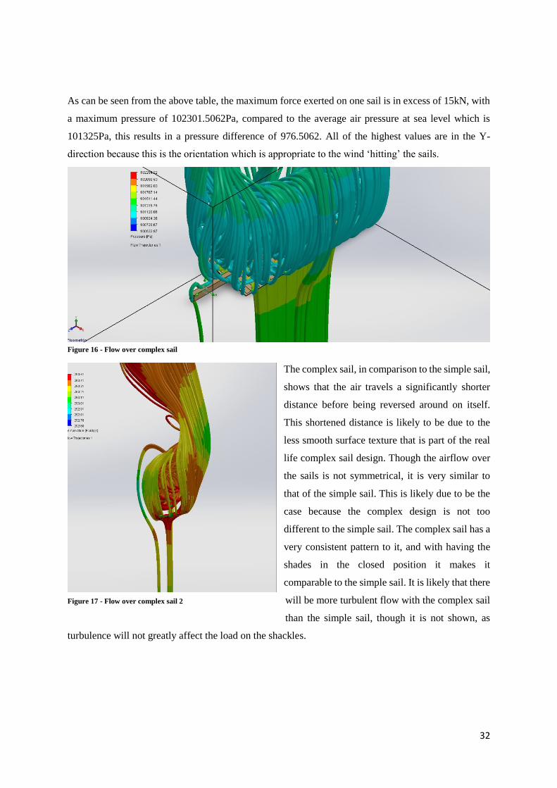
As can be seen from the above table, the maximum force exerted on one sail is in excess of 15kN, with
a maximum pressure of 102301.5062Pa, compared to the average air pressure at sea level which is
101325Pa, this results in a pressure difference of 976.5062. All of the highest values are in the Y-
direction because this is the orientation which is appropriate to the wind ‘hitting’ the sails.
Figure 16 - Flow over complex sail
The complex sail, in comparison to the simple sail,
shows that the air travels a significantly shorter
distance before being reversed around on itself.
This shortened distance is likely to be due to the
less smooth surface texture that is part of the real
life complex sail design. Though the airflow over
the sails is not symmetrical, it is very similar to
that of the simple sail. This is likely due to be the
case because the complex design is not too
different to the simple sail. The complex sail has a
very consistent pattern to it, and with having the
shades in the closed position it makes it
comparable to the simple sail. It is likely that there
will be more turbulent flow with the complex sail
than the simple sail, though it is not shown, as
turbulence will not greatly affect the load on the shackles.
Figure 17 - Flow over complex sail 2
33
Table 6 - Complex sail CFD data
Goal Name Unit Value
Averaged
Value
Minimum
Value
Maximum
Value Delta Criteria
SG Min Static
Pressure
[Pa] 129.8523373 106.7678635 135.4155836 79.69761609 52.17049224 169.8282521
SG Av Static
Pressure
[Pa] 22.54870384 17.74327043 19.08361646 16.11700412 3.34764163 3.577079136
SG Max Static
Pressure
[Pa] 518.0633189 510.0197883 494.3980797 524.9293921 30.53131247 28.00817075
SG Bulk Av
Static Pressure
[Pa] 22.54870384 17.74327043 19.08361646 16.11700412 3.34764163 3.577079136
SG Min Total
Pressure
[Pa] 129.8523373 106.7678635 135.4155836 79.69761609 52.17049224 169.8282521
SG Av Total
Pressure
[Pa] 22.54870384 17.74327043 19.08361646 16.11700412 3.34764163 3.577079136
SG Max Total
Pressure
[Pa] 518.0633189 510.0197883 494.3980797 524.9293921 30.53131247 28.00817075
SG Bulk Av
Total Pressure
[Pa] 22.54870384 17.74327043 19.08361646 16.11700412 3.34764163 3.577079136
SG Normal
Force [N] 757.5818106 542.3088312 360.0600869 623.2437696 342.1374801 819.1810274
SG Normal
Force (X) [N] 191.7312513 113.6024937 65.59900772 141.0866252 80.4217082 180.5695225
SG Normal
Force (Y) [N] 729.9933798 527.3082663 351.2555049 604.3760488 319.525768 799.5643017
SG Normal
Force (Z) [N] 311.6998371 308.7661574 304.5615823 311.7373502 7.304267599 25.54959381
SG Force [N] 760.7579418 545.3743118 363.0396446 626.390703 342.2893829 819.7589748
SG Force (X) [N] 193.1830487 114.2513357 66.64627425 141.5169915 80.34802758 180.2543497
SG Force (Y) [N] 733.1531372 530.5333458 354.2726221 607.7268819 319.2548748 800.2156447
SG Force (Z) [N] 298.5122191 295.543416 291.4439125 298.55613 7.28389812 25.65955056
The above table shows the magnitude of the difference between the simple sail and the complex sail
simulation data. The total pressure that is exerted on the sail is greater on the complex sail than that of
the simple sail, this is likely to do with the fact that the air can flow more freely over the simplified
surface of the plain sail than it can over the realistic complex sail. Air can be trapped locally within the
crevices of the complex sail and then can therefore increase the pressure values that are found in that of
the complex sail over those of the simple sail. The surprising results are that the force is found to be
greater in that of the complex sail than that of the simple designed sail. It was initially thought that a
simple flat plate opposing the wind would provide greater resistance to the wind than a non-flat plate
with identical external dimensions and angles. However, the simulation suggests that this is not the case
as the averaged value is 530N higher in the complex sail than it is in the simple sail, however the
difference in the maximum values is even greater being over 605N greater in the complex sail than in
the simple sail.
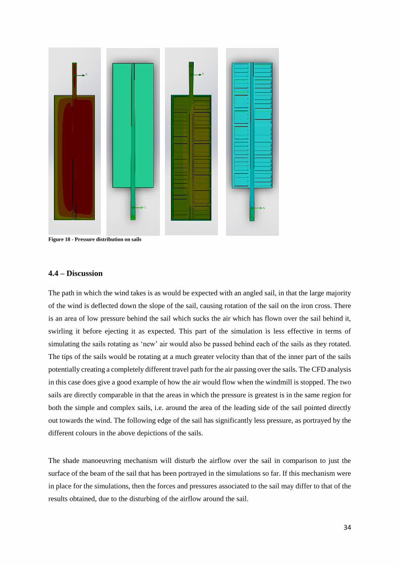
34
4.4 – Discussion
The path in which the wind takes is as would be expected with an angled sail, in that the large majority
of the wind is deflected down the slope of the sail, causing rotation of the sail on the iron cross. There
is an area of low pressure behind the sail which sucks the air which has flown over the sail behind it,
swirling it before ejecting it as expected. This part of the simulation is less effective in terms of
simulating the sails rotating as ‘new’ air would also be passed behind each of the sails as they rotated.
The tips of the sails would be rotating at a much greater velocity than that of the inner part of the sails
potentially creating a completely different travel path for the air passing over the sails. The CFD analysis
in this case does give a good example of how the air would flow when the windmill is stopped. The two
sails are directly comparable in that the areas in which the pressure is greatest is in the same region for
both the simple and complex sails, i.e. around the area of the leading side of the sail pointed directly
out towards the wind. The following edge of the sail has significantly less pressure, as portrayed by the
different colours in the above depictions of the sails.
The shade manoeuvring mechanism will disturb the airflow over the sail in comparison to just the
surface of the beam of the sail that has been portrayed in the simulations so far. If this mechanism were
in place for the simulations, then the forces and pressures associated to the sail may differ to that of the
results obtained, due to the disturbing of the airflow around the sail.
Figure 18 - Pressure distribution on sails
35
4.5 – Conclusion
The anticipated results were that the smooth simple sail, would yield higher results for both the force
and the pressure than that of the complex sail, due to being a larger surface area that is coming into
contact with the wind, but though this was not the case. In fact the opposite was the case, the pressures
and forces were higher in every case in the complex sail over that of the simple sail. This implies that
the design of the sail was more efficient than a plane sail, as more force was able to be exerted through
the same area total area of sail, thereby making the sail with the slats more efficient than that of the
plain sail. The sail with the slats is also capable of opening the slats to allow greater through-flow of
the air through the sail, thereby the reducing the force exerted by the wind, allowing the sail to be
adapted to be functional in higher wind-speeds, this is also ideal in very high wind, or even storm
conditions as even if the mill is stopped the force transferred to the shackles can be minimised by having
the shades open in severe weather conditions.
5. FEA
5.1 – Introduction
This section will be focusing on the Finite element analysis of the shackles used to attach the sails to
the iron cross. The goal of the finite element analysis is to analyse the stress that the shackles are under
and then using this data to give an indication as to why the shackles failed and what could be done to
prevent this happening. Finite element analysis or FEA as it is commonly referred to, is a numerical
method completed on computers that can be used to analyse a wide range of problems. In this case FEA
is used to analyse the stresses and strains that the shackles are put under. The simulations, carried out
on the program ANSYS, give a detailed view of exactly where in the shackles structure stresses are the
greatest. This information is helpful in giving an idea as to why the shackles failed. This section will be
broken down into several parts, a brief background of FEA, a description of the method, results and a
discussion on what the results show.
5.2 – Background
FEA as stated earlier is a numerical method that is completed on computers; it was born from the
aerospace industry in the 50’s and 60’s and has developed ever since (DOBSON, 2013). The capabilities
of FEA software have advanced as the power of computers has advanced. In the early days of FEA only
expensive supercomputers were capable of the calculations so the software was limited to a few
36
industries. But as personal computers have become more affordable and more powerful FEA has
become more accessible. FEA is now a widely used engineering tool used in a variety of different
industries. There are two broad types of FEA 2D and 3D. Both use the same general method. There are
three different stages in obtaining results, pre-processor, solver and post processor. Pre-processor
involves creating the model and defining the parameters of the problem and then creating a mesh and
setting the boundary conditions. Once this is completed the problem is solved by using approximate
functions to formulate linear equations and then solve these equations. The final stage post-processing
involves the using the data obtained from solving the equations to visualise the problem. This can mean
plotting the data in graphs or by using contour plots on the model to help visualise exactly what the data
is showing.
5.3 – Method
The first stage of the FE analysis was to create a 3D CAD model of the system. The software used to
construct the CAD model was SolidWorks. SolidWorks is a 3D computer aided design (CAD) software
which is a fairly common mid-level program. The CAD model that was generated was a simplified
version so that results could be obtained relatively quickly while not deviating too much from the
realistic case. This simplified CAD model included a basic iron cross, a beam and shackles. The basic
versions of the iron cross, sail beam and shackles were constructed on SolidWorks using real life
geometry measurements to get simple models that were as close as possible to the actual components
without being too complex. Once these had been modelled they were assembled together and then
imported into ANSYS, the FEA software. To be more specific the program used was ANSYS
Workbench which is an FEA program that can be linked to SolidWorks. This allows models to be
directly imported from SolidWorks into Workbench. Workbench is a relatively simple program
compared to some other FEA software but it does have limitations, mainly as an automatic mesher is
used it can sometimes be difficult to obtain a mesh to a very high quality. This can have a knock on
effect to results and can lead to inaccuracies. To begin with in ANSYS, a very simple assembly was
used with just two shackles. This assembly was used to test the software to check if it was being set up
correctly. To check if the analysis was set up correctly the stress and deformation were plotted and this
was looked at to see if it was the behaviour that was expected. The first step of an analysis to be carried
out in ANSYS is generating a mesh. Initially this mesh was coarse which gives less accurate results but
speeds up the calculation time. This is useful initially when a simplified system was used but as the
system became more complex a finer mesh had to be used. Once the mesh had been generated the
parameters of the problem were defined. This meant defining the magnitude of the forces and where
they were applied as well as the constraints. There were two forces to consider the weight of the sail
beam and the force generated by the wind. Constraints refer to which part of the model will be fixed in
place. In this case the iron cross was set as being fixed. The contact types also had to be defined. Contact
37
types define what type of contact there is between two surfaces and how the two surfaces will behave
in relation to each other. Contact can be either bonded, no separation, frictionless, frictional or rough
(ANSYS, 2012). The bonded contact type is the most simple as it assumes that there is no separation
between surfaces and no sliding. The next contact type is no separation which again does not allow
surfaces to separate but does allow some sliding. Frictionless, frictional and rough all allow separation
and sliding depending on the coefficient of friction which for frictionless is zero and for rough it is 1.
This means that frictionless is free to slide with no resistance and rough contacts are not allowed to
slide. To make sure the right contact types were used many different cases were experimented with and
the results were checked to see if the system was behaving as expected. If the wrong contacts or
constraints are defined then the solution will either not converge or give incorrect results. There are
several things that could be done to avoid this and to verify if the analysis has been set up correctly. A
modal analysis could be carried out on the system without any forces (HIGGINS, 2012). A modal
analysis vibrates the system, which shows if there is any unwanted movement of the system. Another
way of checking if the system was set up correctly that was used was to just view the deformation and
stress contour plots and use judgement as to whether the system seemed to behaving properly. Once all
of the forces, constraints and contacts have been defined the problem can be solved. Depending on the
complexity of the problem different settings might have to be used. For example if a complex problem
is being solved then the solver may struggle to converge. To help this problem the number of sub steps
and steps can be increased which helps the solver break down the problem. Once the solution has been
found then the software can be used to give the results in the form of a contour plot that helps the data
to be visualised. The contour plots allow the stress of the whole system to be visualised as well as the
stress at any point on the geometry.
5.4 – Results
Several different analysis set ups were used to obtain results. The first, set up 1, was a simple analysis
with weight and wind load (25kN) considered. Solutions for this set up were obtained for three different
orientations, horizontal, vertical up and vertical down. Set up 2 used the same settings as set up 1 but 6
shackles were used instead of 4. Set up 3 used 4 shackles with weight and wind load (15kN) but featured
more complex analysis settings. The 15 kN was a figure obtained from the CFD analysis
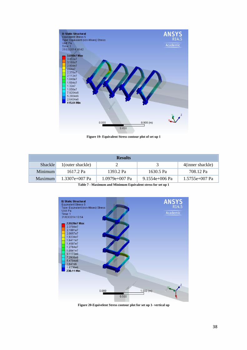
38
Figure 19- Equivalent Stress contour plot of set up 1
Results
Shackle 1(outer shackle) 2 3 4(inner shackle)
Minimum 1617.2 Pa 1393.2 Pa 1630.5 Pa 708.12 Pa
Maximum 1.3307e+007 Pa 1.0979e+007 Pa 9.1554e+006 Pa 1.5755e+007 Pa
Table 7 - Maximum and Minimum Equivalent stress for set up 1
Figure 20-Equivelent Stress contour plot for set up 1- vertical up
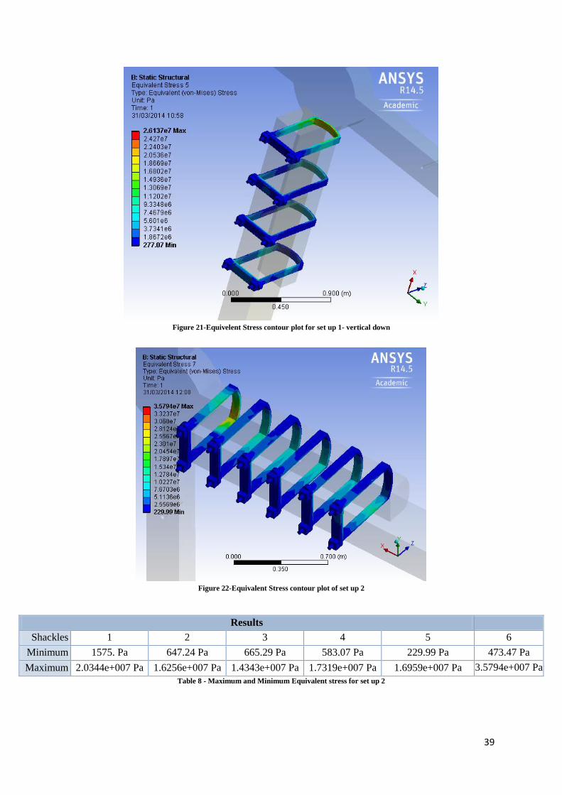
39
Figure 21-Equivelent Stress contour plot for set up 1- vertical down
Figure 22-Equivalent Stress contour plot of set up 2
Results
Shackles 1 2 3 4 5 6
Minimum 1575. Pa 647.24 Pa 665.29 Pa 583.07 Pa 229.99 Pa 473.47 Pa
Maximum 2.0344e+007 Pa 1.6256e+007 Pa 1.4343e+007 Pa 1.7319e+007 Pa 1.6959e+007 Pa 3.5794e+007 Pa
Table 8 - Maximum and Minimum Equivalent stress for set up 2
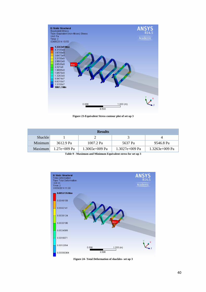
40
Figure 23-Equivalent Stress contour plot of set up 3
Results
Shackle 1 2 3 4
Minimum 3612.9 Pa 1007.2 Pa 5637 Pa 9546.8 Pa
Maximum 1.27e+009 Pa 1.3065e+009 Pa 1.3027e+009 Pa 1.3263e+009 Pa
Table 9 - Maximum and Minimum Equivalent stress for set up 3
Figure 24- Total Deformation of shackles- set up 3
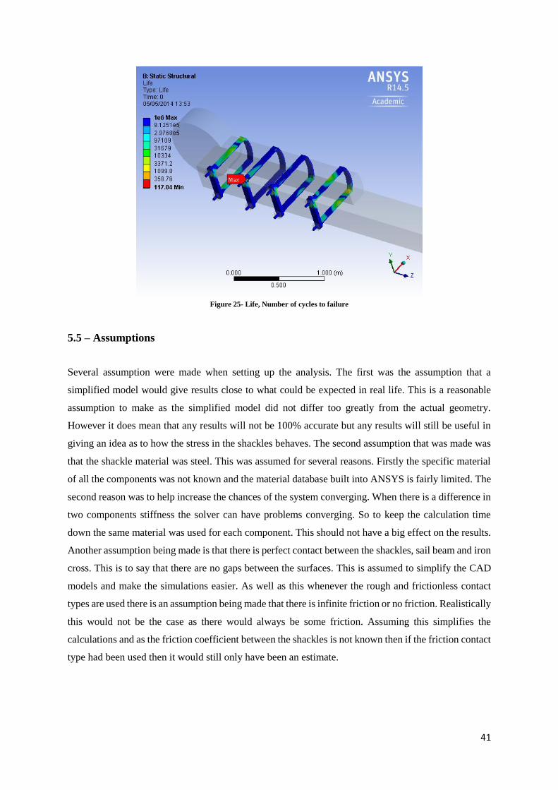
41
Figure 25- Life, Number of cycles to failure
5.5 – Assumptions
Several assumption were made when setting up the analysis. The first was the assumption that a
simplified model would give results close to what could be expected in real life. This is a reasonable
assumption to make as the simplified model did not differ too greatly from the actual geometry.
However it does mean that any results will not be 100% accurate but any results will still be useful in
giving an idea as to how the stress in the shackles behaves. The second assumption that was made was
that the shackle material was steel. This was assumed for several reasons. Firstly the specific material
of all the components was not known and the material database built into ANSYS is fairly limited. The
second reason was to help increase the chances of the system converging. When there is a difference in
two components stiffness the solver can have problems converging. So to keep the calculation time
down the same material was used for each component. This should not have a big effect on the results.
Another assumption being made is that there is perfect contact between the shackles, sail beam and iron
cross. This is to say that there are no gaps between the surfaces. This is assumed to simplify the CAD
models and make the simulations easier. As well as this whenever the rough and frictionless contact
types are used there is an assumption being made that there is infinite friction or no friction. Realistically
this would not be the case as there would always be some friction. Assuming this simplifies the
calculations and as the friction coefficient between the shackles is not known then if the friction contact
type had been used then it would still only have been an estimate.
42
5.6 – Limitations
There were several different limitations limiting the kind of results that could be obtained. The first
limitation and possibly the biggest was time. For very simple analyses, calculations can be carried out
quickly. But for more complex analyses the calculation time can be much longer. As well as the
calculation times another thing that contributed to limiting the time was the fact that the software was
only available on university computers which limited the possible computer time. Another limitation
was the computing power available. With some of the more complex calculations the computer would
struggle to converge on a solution. This meant that the complexity of the analysis had to be kept down
which meant the results that could be gathered were limited. The final thing limiting what could be
achieved was a lack of experience in FEA stress analysis. To be fully proficient in carrying out stress
analysis engineers train for years, which was obviously not feasible for a project of this length.
5.7 – Discussion
As shown in the results section several different simulation set ups were used. The most simple of these
was used initially to get some early results to give an idea of what to expect and to gain some familiarity
with the software. To keep the calculations relatively short the main contact type used between the
components was bonded. Using bonded speeds up the calculations as it keeps the system linear which
simplifies the calculations (HIGGINS, 2012). Bonded contact means that two surfaces are effectively
glued together so they cannot separate or slide. This is obviously not how the system would behave in
the real world as in reality the sail beam is likely to want to pivot about the iron cross and would not be
bonded to the surface of the iron cross. The results obtained from this while not completely correct were
useful in giving an idea of what could be expected from more complex cases. One thing that was
indicated by these early results was that the worst loading case was when the sail beam was horizontal.
The horizontal had higher stresses than the vertical up and vertical down loading cases. This is not too
surprising as due to moments the force produced by the weight of the sail beam will be the greatest
when it is horizontal. The maximum stresses in each bracket for this simplified system were found to
be an average of 2.3x10^7 Pa or 23MPa, as shown in figure 19, which is not too far of what could be
expected. This stress was calculated using both the weight of the sail and a wind force of 25kN. This
wind load was chosen as it was a reasonable estimated worst case scenario. The reason these results are
not too useful is how the system behaved. The stress distribution across the shackles was uneven. The
results showed large areas of very low stress. This would indicate that the system is not behaving
correctly as it would be expected that every area of the shackle to be under some stress. The stress
across wide areas of the shackles was as low as about 400 Pa whereas the areas of high stress were to
the order of 10^7 Pa. Using the same analysis settings a model with 6 shackles was analysed. This was
done to see what effect adding extra shackles would have and if that would be a viable option for
43
preventing failure in the future. The results showed that the stress was lowered by adding more shackles
but the amount it was lowered by was relatively small. The average peak stress was found to have
reduced by about 3%. This is a much smaller reduction than was expected. This could be due to the
simplified nature of the system and further indicates that the simplified system does not behave
realistically.
The next set of results were obtained using more realistic contact types. The most realistic case used
was a frictionless contact between the beam and the iron cross and rough contacts between the shackles,
the beam and the iron cross. This is a logical set up that is the most similar to reality without being
overly complex. When using this set up the results appeared to behave as expected. There was a greater
stress on the first and last shackle and the areas of high stress were where they would be expected to be
as shown by figure 23. This indicated that the beam was moving as it should do and the shackles were
constraining the beam as they should do. However this set of results showed that there was a small area
of very high stress, about 1.3x10^9 Pa or 1300 MPa. This is very high and well over the yield strength
of some mild steels. Due to the fact that the stress in this area is so much higher than all the other areas,
a whole magnitude higher, it is likely an anomaly. This is also supported by the fact that the area of
stress that is at that level is very small and almost seems to be just a point. There are several thing things
that could have caused this anomaly but the most likely is due to a bad mesh. The area that is shown to
have this high stress is where two components meet. The mesh sizes of these two components were
different and changed fairly abruptly which can lead to errors. If this peak stress is ignored then the
areas of highest stress are in the corners of the shackles as could be expected (LOZZI, 2014). In the
corners the stress was shown to be about 5x10^8 Pa which a much more reasonable stress. In general
the stress in the shackles was within the region of 1.3x10^7 to 1x10^8 with the minimum stress being
as low as 1000 Pa. Depending on which grade of steel is used the ultimate tensile strength is in the
range of 372MPa to 2310MPa for medium alloy steels and even higher for higher grade steel. This
means that the stresses calculated should not be exceeding the ultimate tensile strength, the point at
which a material will break, under the loading conditions used. There is likely to be some error with
these figures due to the way the system was constrained and the materials used for the analysis. For the
analysis the iron cross was completely fixed which in reality it would not be. It would be able to deform
slightly. This should not have a big effect on the results but it could have some influence. This was
expected as the shackles historically have not failed because of the stress being too high, they have
failed either because of poor manufacturing or possibly due to fatigue. Fatigue is important to consider
as it takes into account the effects of cyclic loading. Cyclic loading can cause cracks to form and grow
slowly until the point at which fast fracture will occur and the material will fail. Figure 25 shows a plot
of the calculated life of the shackles. It shows in the areas of low stress, low cycle fatigue is not a
concern with a life of 1x10^6 cycles. But in the areas such as the corners where the stress concentrations

44
were the life fell to about 1000 cycles. This is very low, however this was calculated using a fully
reversed model meaning that the forces were inverted each cycle. This would be close to realistic if
only the sail weight was included, but this calculation inverted the wind load as well. This would not
occur in the real world as the wind would not be likely to flip direction repeatedly and the sails would
turn into the wind.
5.8 – Conclusion
In conclusion, in general the simulations behaved somewhat predictably. The initial results gathered
using a simplified system showed some correct behaviour but also some unexpected results. The more
complex system performed much better and exhibited behaviour very close to what would be expected
in reality. Limitations in time and computing power meant that not a great deal of complex cases could
be examined within the given time frame. When a complex system was used the results showed a stress
in the region that would be expected with concentrations in the corners. The results of the complex
system showed that stress tended to be within in the region of 1.3x10^7 to 1x10^8 which should be an
acceptable amount depending on the material and manufacturing methods used. With the ultimate
tensile strength of steel ranging from 372-2310MPa this means that if the correct material is chosen
then there should not be an issue of the shackle failing quickly. Ideally a material with a yield strength
of about 500MPa would be used. Depending on allowable budget this may or may not be feasible. There
is however still a risk of failing due to the stress concentrations in the corners and by fatigue. The stress
concentrations in the corners of the shackles are at a level that depending on the material could be above
the yield strength. This can cause deformations that can open up cracks that will propagate (FANCEY,
2012). For this reason the way the shackles are manufactured has to be chosen carefully. The corners
need to have a smooth transition and material flaws need to be avoided if possible. This would reduce
the chance of cracks propagating. Fatigue is also a risk due to the cyclic nature of the loading when the
windmill is turning. The exact life of the shackles was not determined however the results did show that
fatigue would be a factor. To prevent these failures from occurring, more shackles could be added which
would lower the stress, although by how much was not properly determined. Another possibility would
be to increase the shackle thickness at the areas of high stress. Depending on how the shackles are
manufactured this could be feasible. However it is hard to say for certain how much material would
need to be added without more time being spent gathering detailed solutions.
45
6. Power output
6.1 – Introduction
This section will be based on the calculation and comparison of power output between a traditional
windmill and wind turbine. In general power out of a windmill depends on the efficiency of the windmill,
the height and area swept by the sails and the wind speed. This mean for a windmill to generate a high
power output, both the speed and force of the wind can be significant factors. The more wind speed and
force you have got, the greater is the amount of power your wind mill generates. Different regions have
different wind speeds. The amount of power produced by your wind mill is proportional to the size of
the rotor sails or area swept, when all other factors have been taken into consideration. A bigger rotor
certainly generates more power. For a wind turbine, the rotor swept area, A, is important because the
rotor is the part of the turbine that captures the kinetic wind energy. So, the larger the rotor, the more
energy it can capture from the wind. “The fact that the power is proportional to the cube of the wind
speed is very significant. This can be demonstrated by pointing out that if the wind speed doubles then
the power in the wind increases by a factor of eight”. (Action, NA)
In this section it is predicted that the power output generated by a traditional windmill will much lesser
than of medium wind turbine. This is because they are less efficient with their non-aerodynamics sails,
and the rotor sails are usually smaller compared to that of the wind turbine rotor blade.
6.2 – Calculations
Assumption
To calculate the power output of a traditional windmill it is assumed coefficient of performance (Cp) of
around 0.17 to 0.20 due to the four non-aerodynamic sails. This means that up to 17-20 % of the
available kinetic energy in the wind flowing through the area swept by the sails can be converted to
torque on the wind-shaft.
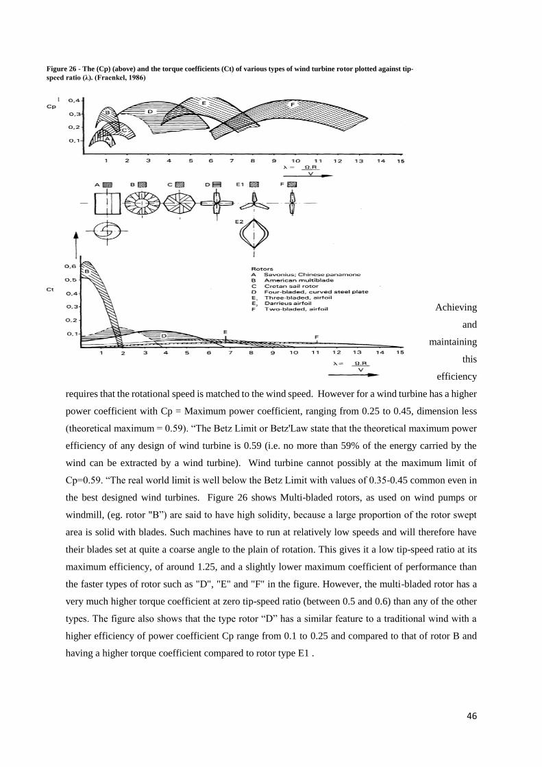
46
Achieving
and
maintaining
this
efficiency
requires that the rotational speed is matched to the wind speed. However for a wind turbine has a higher
power coefficient with Cp = Maximum power coefficient, ranging from 0.25 to 0.45, dimension less
(theoretical maximum = 0.59). “The Betz Limit or Betz'Law state that the theoretical maximum power
efficiency of any design of wind turbine is 0.59 (i.e. no more than 59% of the energy carried by the
wind can be extracted by a wind turbine). Wind turbine cannot possibly at the maximum limit of
Cp=0.59. “The real world limit is well below the Betz Limit with values of 0.35-0.45 common even in
the best designed wind turbines. Figure 26 shows Multi-bladed rotors, as used on wind pumps or
windmill, (eg. rotor "B”) are said to have high solidity, because a large proportion of the rotor swept
area is solid with blades. Such machines have to run at relatively low speeds and will therefore have
their blades set at quite a coarse angle to the plain of rotation. This gives it a low tip-speed ratio at its
maximum efficiency, of around 1.25, and a slightly lower maximum coefficient of performance than
the faster types of rotor such as "D", "E" and "F" in the figure. However, the multi-bladed rotor has a
very much higher torque coefficient at zero tip-speed ratio (between 0.5 and 0.6) than any of the other
types. The figure also shows that the type rotor “D” has a similar feature to a traditional wind with a
higher efficiency of power coefficient Cp range from 0.1 to 0.25 and compared to that of rotor B and
having a higher torque coefficient compared to rotor type E1 .
Figure 26 - The (Cp) (above) and the torque coefficients (Ct) of various types of wind turbine rotor plotted against tip-
speed ratio (λ). (Fraenkel, 1986)
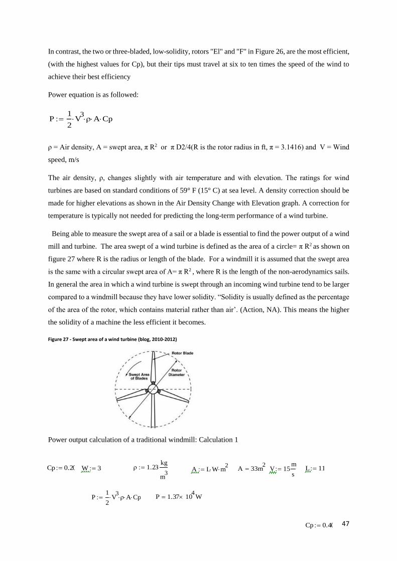
47
In contrast, the two or three-bladed, low-solidity, rotors "El" and "F" in Figure 26, are the most efficient,
(with the highest values for Cp), but their tips must travel at six to ten times the speed of the wind to
achieve their best efficiency
Power equation is as followed:
ρ = Air density, A = swept area, π R2 or π D2/4(R is the rotor radius in ft, π = 3.1416) and V = Wind
speed, m/s
The air density, ρ, changes slightly with air temperature and with elevation. The ratings for wind
turbines are based on standard conditions of 59° F (15° C) at sea level. A density correction should be
made for higher elevations as shown in the Air Density Change with Elevation graph. A correction for
temperature is typically not needed for predicting the long-term performance of a wind turbine.
Being able to measure the swept area of a sail or a blade is essential to find the power output of a wind
mill and turbine. The area swept of a wind turbine is defined as the area of a circle= π R2 as shown on
figure 27 where R is the radius or length of the blade. For a windmill it is assumed that the swept area
is the same with a circular swept area of A= π R2 , where R is the length of the non-aerodynamics sails.
In general the area in which a wind turbine is swept through an incoming wind turbine tend to be larger
compared to a windmill because they have lower solidity. “Solidity is usually defined as the percentage
of the area of the rotor, which contains material rather than air’. (Action, NA). This means the higher
the solidity of a machine the less efficient it becomes.
Figure 27 - Swept area of a wind turbine (blog, 2010-2012)
Power output calculation of a traditional windmill: Calculation 1
P1
2V
3 A Cp
1.23kg
m3
A L W m2
A 33m2
V 15m
s L 11W 3
P1
2V
3 A Cp P 1.37 10
4 W
Cp 0.20
Cp 0.40
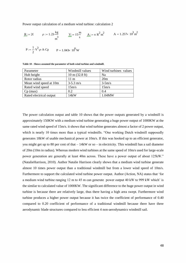
48
Power output calculation of a medium wind turbine: calculation 2
Table 10 - Shows assumed the parameter of both wind turbine and windmill.
Parameter Windmill values Wind turbines values
Hub height 10 m (32.8 ft) Na
Rotor radius 11 m 20m
Mean wind speed at 10m 3-5.3 m/s 3-5m/s
Rated wind speed 15m/s 15m/s
Cp (max) 0.2 0.4
Rated electrical output 14kW 1.04MW
The power calculation output and table 10 shows that the power outputs generated by a windmill is
approximately 150KW with a medium wind turbine generating a huge power output of 1000KW at the
same rated wind speed of 15m/s. it shows that wind turbine generates almost a factor of 2 power output,
which is nearly 10 times more than a typical windmills. “One working Dutch windmill supposedly
generates 18kW of usable mechanical power at 10m/s. If this was hooked up to an efficient generator,
you might get up to 80 per cent of that – 14kW or so – in electricity. This windmill has a sail diameter
of 20m (10m in radius). Whereas modern wind turbines at the same speed of 10m/s used for large-scale
power generation are generally at least 40m across. These have a power output of about 125kW.”
(NatalieHarrison, 2010). Author Natalie Harrison clearly shows that a medium wind turbine generate
almost 10 times power output than a traditional windmill but from a lower wind speed of 10m/s.
Furthermore to support the calculated wind turbine power output. Author (Action, NA) states that ‘for
a medium wind turbine ranging 12 m to 45 m can generate power output 40 kW to 999 kW which’ is
the similar to calculated value of 1000KW. The significant difference to the huge power output in wind
turbine is because there are relatively large, thus there having a high area swept. Furthermore wind
turbine produces a higher power output because it has twice the coefficient of performance of 0.40
compared to 0.20 coefficient of performance of a traditional windmill because there have three
aerodynamic blade structures compared to less efficient 4 non-aerodynamics windmill sail.
A R2
m2
A 1.257 103
m2
R 20 1.23kg
m3
V 15m
s
P1
2V
3 A Cp P 1.043 10
6 W
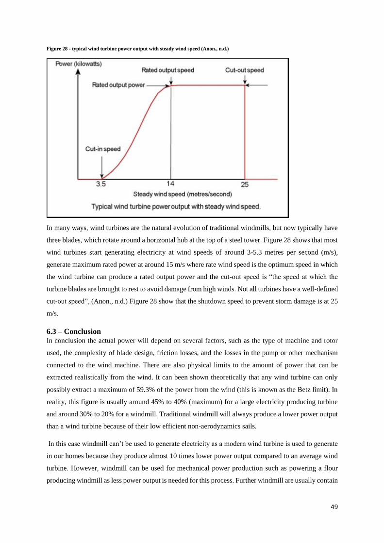
49
Figure 28 - typical wind turbine power output with steady wind speed (Anon., n.d.)
In many ways, wind turbines are the natural evolution of traditional windmills, but now typically have
three blades, which rotate around a horizontal hub at the top of a steel tower. Figure 28 shows that most
wind turbines start generating electricity at wind speeds of around 3-5.3 metres per second (m/s),
generate maximum rated power at around 15 m/s where rate wind speed is the optimum speed in which
the wind turbine can produce a rated output power and the cut-out speed is “the speed at which the
turbine blades are brought to rest to avoid damage from high winds. Not all turbines have a well-defined
cut-out speed”, (Anon., n.d.) Figure 28 show that the shutdown speed to prevent storm damage is at 25
m/s.
6.3 – Conclusion
In conclusion the actual power will depend on several factors, such as the type of machine and rotor
used, the complexity of blade design, friction losses, and the losses in the pump or other mechanism
connected to the wind machine. There are also physical limits to the amount of power that can be
extracted realistically from the wind. It can been shown theoretically that any wind turbine can only
possibly extract a maximum of 59.3% of the power from the wind (this is known as the Betz limit). In
reality, this figure is usually around 45% to 40% (maximum) for a large electricity producing turbine
and around 30% to 20% for a windmill. Traditional windmill will always produce a lower power output
than a wind turbine because of their low efficient non-aerodynamics sails.
In this case windmill can’t be used to generate electricity as a modern wind turbine is used to generate
in our homes because they produce almost 10 times lower power output compared to an average wind
turbine. However, windmill can be used for mechanical power production such as powering a flour
producing windmill as less power output is needed for this process. Further windmill are usually contain
50
a higher solidity properties, carrying a lot of material and have coarse sails angles which inherently less
efficient than low-solidity machines. This means windmill are more likely to have a higher twisting or
rotary force by the rotor (which is called torque) and be able to rotate the mechanical mechanism and
gears to produce the flours. However to generate electricity the properties of the machine have to have
low solidity which tend to run at a higher speed generating a much lower starting torque. Wind turbine
are used to generate electricity because of they have a higher tip-speed ration as shown on figure 27.
Wind turbines are designed with optimal tip speed ratios to get the maximum amount of power from
the wind. If the rotor of the windmill spins too slowly, most of the wind will pass straight through the
gap between the blades, therefore giving little or no power output. But wind turbine have a high tip
speeds which will spin fast enough to get the maximum amount of power from the wind. Thus if the
rotor spin too fast the blades will blur and acts like a solid wall to the wind creating a turbulence flow
as they spin through the air reducing power input from the air when the next blades arrives too quickly
hitting the turbulent air.
7. Project management
As is shown by the two Gantt charts shown in tables 1 and 13, found in the appendices, there is a
differences between what was planned and what was achieved during this project. A change was
expected as this type of project rarely follows the plan exactly. As a project is being completed new
ideas are thought of constantly and the project is inevitably taken in a slightly different direction. In this
case the project got off to a slow start due to a lack of accurate information regarding the windmill
dimensions. The site visit that was used to obtain this information took place several weeks later than
planned and this had a knock on effect on the other aspects of the project. The lack of accurate
dimensions meant that the models produced were just estimates making it difficult to proceed with the
analyses. Another reason for the project not progressing as quickly as was initially expected was
unforeseen issues with software. It was underestimated how long the period of software familiarisation
would take and how long some of the calculations would take. The amount that could be accomplished
on the software was also overestimated during the planning stage. The complexity of the FEA software,
for example, was underestimated. This meant that what was originally thought of as being a relatively
simple analysis, was actually much more complex and therefore time consuming. All of this contributed
to the fact that what was actually achieved and what was planned differed by the end of the project. To
try and keep the project on the right track there were regular group meetings to make sure all members
of the group were on the right track and that
51
8. Final Discussion
After having utilised the CFD to calculate the forces that the sails will experience, both a simplified,
plain, flat sail, and an accurate model as close to the real sail as possible were analysed. It was
discovered that a simplified sail will not suffice to be a representation of the Skidby windmill, due to
the differences in the results obtained between the two models. For a highly over anticipated wind-
speed of 25m/s, the maximum possible force that the sail will experience is 15347.89918N. This
therefore means that the absolute maximum simulated wind-force that must be dealt with by the
shackles is 15347.89918N, though no one shackle should have to deal with all of the load from the sail,
and is spread over four shackles.
This then lead onto the potential new designs as to how the sails can be held onto the iron-cross. Some
adaptations of the original design were proposed, which were more cost effective, or easier to install,
or replace, as well as other more adventurous designs which had their bases in other industries. The
designs were proposed and presented to the officials who are responsible for the maintenance of the
mill, however the mill is a historically graded II* listed building and therefore its components must
match and suit the grade of the building, and fit into the era in which it was built. This therefore limited
what could be done with the designs, and ruled out an alternate, completely different shackle design. It
was therefore essential to keep the shackle design very close to the original, maybe even to just a slight
modification, or refinement of the original design, or perhaps even a change to a different material. A
different material is a viable option, because the shackles on the windmill are painted red, and so it
would be unnoticeable to the public that a material had changed.
Though other materials were considered, a form of steel was the only viable option that was tailored to
all the strength, size, lifespan, ease of manufacture, reparability and fatigue resistance. Corrosion
resistance was the only potential problem with steel, with the wet climate of East Yorkshire is exposed
to. The solution of stainless steel was dismissed due to the cost being five times greater than that of
alloy steel, and the shackles could be painted instead, achieving a similar corrosion resistance but
requiring less maintenance.
For the FEA steel was the material examined, and so the analysis consisted only of various different
grades of steel. The most realistic results were obtained when the contact between the sail beam and the
iron cross were perceived to be frictionless, with ‘rough’ contacts given between the shackles and both
the sail beam, and the iron cross. The most realistic results were obtained because this is the most
realistic set-up as to how the sail beam – iron cross – shackles interfaces are in real life. The stress
values obtained were of a reasonable magnitude, between 10^7Pa and 10^8Pa, which is below the yield
52
stress of most, if not all types of steel. Adding more identical brackets to the system did reduce the
stress placed on the bracket, but by much less than is anticipated, only approximately 3% reduction in
the most part of the stress, and so makes for questioning the worth of adding more brackets. The life
cycle of a bracket was in the order of 10^6 cycles, which is too few cycles as at that, the brackets will
last less than a half year, when operating at 5 hours a day every day, which is not unreasonable duration
for the windmill to be active per day, although it is doubtful that the mill will be in operation every day.
This value of 10^6 was all that ANSYS was able to produce data for on the computer used, hence the
actual number of cycles until failure may be higher again.
9. Conclusion
Although the shackles could be improved upon, in that the design could be altered, the attachment
method could be different, and the material could be changed it remained similar due to the necessity
to conform to the grade II* listed status of Skidby Mill. Hence only small alterations to the design of
the shackles can be suggested. Though no simple trending statistics were obtained, the stress
concentrations were always highest at the corners of the U-shaped shackles. The stress concentrations
were highest on the inside corners of the U on the shackles that are the furthest from the centre of the
iron cross, and highest on the outside of the corner of the U on the shackles closest in to the iron cross.
Though the stress concentrations were found to be on opposite sides of the shackle, they were in the
same localised area, namely, the corner of the shackle. A straight piece of 20mm thick steel, bent into
the appropriate U-shape, is not sufficient with the localised stresses, it is therefore advised that around
the corners of the U-shape, the material is thicker at the corners. This increase in thickness can be
achieved numerous ways, the gauge of the steel could be increased for the entirety of the shackle,
although this would make bending the shackle to the desired shape more difficult, and for the majority
of the shackle, the 20mm thickness was more than sufficient as it was. The shackle could be tapered to
have an increased thickness at the corners of the shackle, it would still be more difficult to bend into
shape, but this is the most material effective solution. One final option would be to continue with an
initial, standard, 20mm thick steel shackle, and to weld gusseting to the corners of the U-shape after it
has been bent into shape, this would be the most cost effective solution. Exactly how much thicker the
corners need to be than the rest of the U-shape is not known, due to computational limitations, but an
increase in thickness at the corners will only increase lifespan of the shackles.
53
10. Future work
If this project were to be continued in the future there are several different things that could be achieved
if more time was available. Firstly, more detailed stress analysis could be carried out with the eventual
goal of being able to submit design recommendations to east riding of Yorkshire council. For this to
happen the effects of fatigue in particular would need to be analysed in much more detail. Ideally this
would mean being able to confidently say the expected life of the current shackle designs and being
able to determine with confidence exactly how they are likely to fail. This information would then be
combined with the materials and manufacture study to try and determine how any potential weaknesses
could be solved. With more detailed results a specific material could be recommended that would fit
the council’s needs. As well as further developing the FEA, the materials and manufacture section could
be developed further by going into more detail about historic materials and manufacture methods versus
the modern day methods that would be used. This would be an interesting study to find if the modern
day methods have actually improved since the 17th century. As well as this more specific manufacturing
methods could researched, for example the possibilities of machining the shackles. Ideally by the end
of the manufacturing study the most suitable method of manufacturing the shackles could be
recommended. For the CFD section, a complete windmill could be analysed. This would include the
structure of the windmill to see what the effects it has on the forces involved. This would require much
more complex CAD models and longer simulation times.
11. References
East riding of Yorkshire council. About Skidby Mill. (Online) Available at:
<http://www.museums.eastriding.gov.uk/skidby-mill/about-skidby-mill/> [Accessed 27 January
2014].

54
East riding of Yorkshire council 1. Skidby Windmill information sheet. (Online PDF). Available at:
<http://www.museums.eastriding.gov.uk/skidby-mill/mill-history/> [Accessed 28 January 2014].
East riding of Yorkshire council 1a. Skidby Windmill information sheet. (image Online PDF).
Available at: <http://www.museums.eastriding.gov.uk/skidby-mill/mill-history/> [Accessed 28
January 2014].
East riding of Yorkshire council 2. Skidby Windmill information sheet. ( Online ). Available at: <
http://www.museums.eastriding.gov.uk/skidby-mill/our-flour/ > [Accessed 27 January 2014].
East riding of Yorkshire council. Skidby Windmill information sheet. ( image Online pdf ). Available
at: < http://www.museums.eastriding.gov.uk/skidby-mill/learning/ > [Accessed 27 January 2014].
East riding of Yorkshire council 3a. How wind works. ( Online pdf ). Available at: <
http://www.museums.eastriding.gov.uk/skidby-mill/learning/ > [Accessed 27 January 2014].
Wikipedia., 2009 Tower mill. (Online) Available at:< http://en.wikipedia.org/wiki/Tower_mill >
[Accessed 27 January 2014].
East riding of Yorkshire council 4. East riding Mills. ( Online pdf ). Available at: <
http://www.museums.eastriding.gov.uk/skidby-mill/learning/ > [Accessed 05 February 2014].
Wikipedia 2., 2010 Revision history of "Windmill. (Online) Available at :<
http://simple.wikipedia.org/wiki/Windmill > [Accessed 27 January 2014]
https://www.SolidWorks.com/sw/docs/Corp_FactSheet_2012Q2.pdf
ANSYS. (2012) ANSYS Mechanical User Guide. [Online] Available from:
http://www.mecheng.osu.edu/documentation/Fluent14.5/145/wb_sim.pdf [Accessed:05/05/2014]
MATWEB. (2014) Overview of materials for Medium Alloy Steel. [Online] Available from-
http://www.matweb.com/search/DataSheet.aspx?MatGUID=f7666326ceb3482f87a9f41ace1d1fb0
[Accessed:05/05/2014]
FANCEY, K. (2012) Materials and Manufacturing ll, 57017. [Lecture notes] Fatigue. Design,
Materials and Manufacture Module. University of Hull, Applied science, West Lecture theatre,
October 2012.
DOBSON, C. (2013) Finite Element Analysis, 57041. [Lecture notes] Introduction to Finite Element
Analysis, Stress analysis and FEA Module. University of Hull, Larkin, Lecture theatre D, October
2013
HIGGINS, J. (2012). Obtaining and Optimizing Structural Analysis Convergence. [Online] May
2012. Available from:
http://www.ansys.com/staticassets/ANSYS/Conference/Confidence/Boston/Downloads/obtaining-
and-optimizing-convergence.pdf [Accessed: 05/05/2014]
LOZZI, A. (2014) Introduction to Finite Element Analysis. [Online] Available from:
http://web.aeromech.usyd.edu.au/MECH4460/Course_Documents/FEA/Lecture%20intro%20to%20F
EA%20d.pdf [Accessed:05/05/14]
2, w., 2007. Titanium. [Online]
Available at: http://en.wikipedia.org/wiki/Titanium
[Accessed 16 march 2014].
Aalco, 2014. Introduction to Aluminium and its alloys. [Online]
Available at: http://www.aalco.co.uk/datasheets/Aluminium-Alloy_Introduction-to-Aluminium-and-
its-alloys_9.ashx
[Accessed 1 march 2014].
Anon., 2003. Brittle and Ductile Behavior. [Online]
Available at: http://dolbow.cee.duke.edu/TENSILE/tutorial/node10.html
[Accessed 2014 April 24].
55
B, S. B. /. J. Y. /. S. S. /. M. /. K., 2009. Material Science Material Science Material Science---
MECH 2104. [Online]
Available at:
http://www.uom.ac.mu/faculties/foe/mped/students_corner/notes/enggmaterials/steelbklet.pdf
[Accessed 28 April 2014].
defects, W., n.d. Welding defects. [Online]
Available at: http://mercury.kau.ac.kr/welding/Welding%20Technology%20II%20-
%20Welding%20Metallurgy/Chapter%209%20-%20Welding%20Defects.pdf
[Accessed 1 March 2014].
Gandy, D., 2007 . Carbon Steel handbook, USA: ELECTRIC POWER RESEARCH INSTITUTE.
handbook, e., 2004 - 2006. Engineering Materials. [Online]
Available at: http://www.engineershandbook.com/Materials/mechanical.htm
[Accessed 3 march 2014].
Jackson, W. J. .., n.d. FRACTURE TOUGHNESS IN RELATION TO STEEL CASTING DESIGN AND
APPLICATION. [Online]
Available at: http://www.sfsa.org/sfsa/pubs/misc/Fracture%20Toughness.pdf
[Accessed 20 April 2014].
Kumar, P. S. K. a. P. A., n.d. Design of Steel Structures. [Online]
Available at: http://nptel.ac.in/courses/IIT-
MADRAS/Design_Steel_Structures_I/1_introduction/3_properties_of_steel.pdf
[Accessed 1 March 2014].
made, H. p. a., 2000. Titanium background. [Online]
Available at: http://www.madehow.com/Volume-7/Titanium.html#ixzz30TCj6UEV
[Accessed 20 April 2014].
NA, 2001. strength-toughness. [Online]
Available at: http://www-materials.eng.cam.ac.uk/mpsite/interactive_charts/strength-
toughness/NS6Chart.html
[Accessed 20 April 2014].
Packard, K., 2009. [Online]
Available at: http://www.thefabricator.com/article/consumables/understanding-low-alloy-steel
[Accessed 16 April 2014].
Trail, B. a. S., 1996. STRUCTURAL INTEGRITY ASSESSMENT PROCEDURES, London: British
Steel plc.
TYNE, C. V., 2013. forging materials- Plain-Carbon and Low-Alloy Steels. [Online]
Available at: http://www.forgemag.com/articles/83794-forging-materials-plain-carbon-and-low-alloy-
steels
[Accessed 28 April 2014].
WebElements, n.d. Aluminium: the essentials. [Online]
Available at: http://www.webelements.com/aluminium/
[Accessed April 24 2014].
Wikipedia, 2010. [Online]
Available at: http://en.wikipedia.org/wiki/Mild_steel#Mild_steel
[Accessed 23 April 2014].
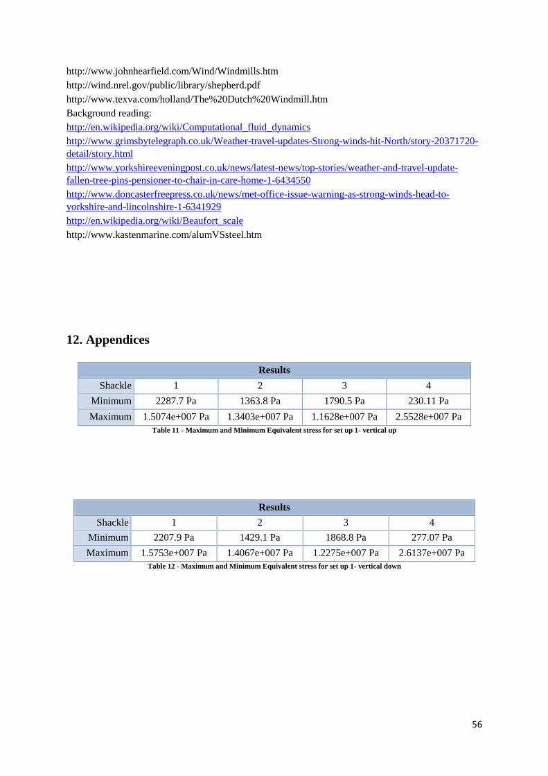
56
http://www.johnhearfield.com/Wind/Windmills.htm
http://wind.nrel.gov/public/library/shepherd.pdf
http://www.texva.com/holland/The%20Dutch%20Windmill.htm
Background reading:
http://en.wikipedia.org/wiki/Computational_fluid_dynamics
http://www.grimsbytelegraph.co.uk/Weather-travel-updates-Strong-winds-hit-North/story-20371720-
detail/story.html
http://www.yorkshireeveningpost.co.uk/news/latest-news/top-stories/weather-and-travel-update-
fallen-tree-pins-pensioner-to-chair-in-care-home-1-6434550
http://www.doncasterfreepress.co.uk/news/met-office-issue-warning-as-strong-winds-head-to-
yorkshire-and-lincolnshire-1-6341929
http://en.wikipedia.org/wiki/Beaufort_scale
http://www.kastenmarine.com/alumVSsteel.htm
12. Appendices
Results
Shackle 1 2 3 4
Minimum 2287.7 Pa 1363.8 Pa 1790.5 Pa 230.11 Pa
Maximum 1.5074e+007 Pa 1.3403e+007 Pa 1.1628e+007 Pa 2.5528e+007 Pa
Table 11 - Maximum and Minimum Equivalent stress for set up 1- vertical up
Results
Shackle 1 2 3 4
Minimum 2207.9 Pa 1429.1 Pa 1868.8 Pa 277.07 Pa
Maximum 1.5753e+007 Pa 1.4067e+007 Pa 1.2275e+007 Pa 2.6137e+007 Pa
Table 12 - Maximum and Minimum Equivalent stress for set up 1- vertical down
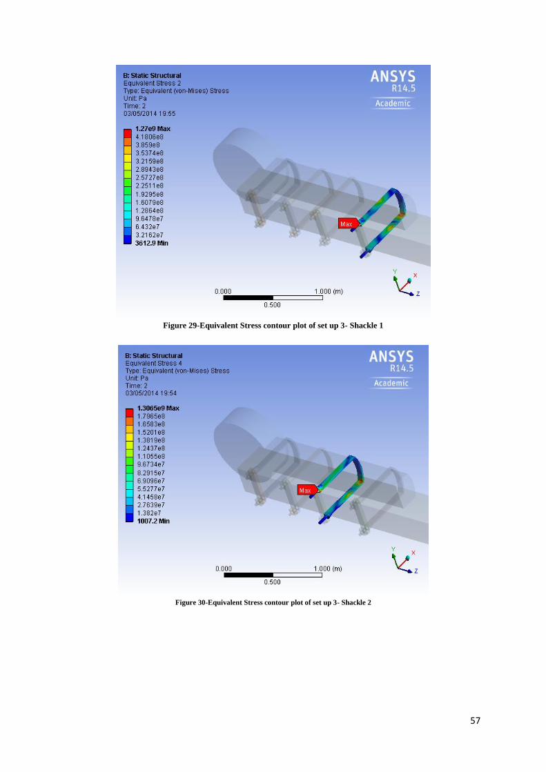
57
Figure 29-Equivalent Stress contour plot of set up 3- Shackle 1
Figure 30-Equivalent Stress contour plot of set up 3- Shackle 2
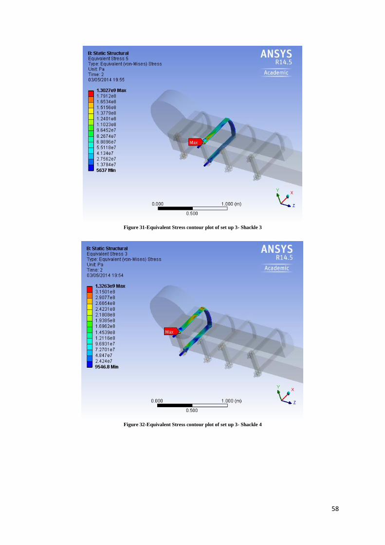
58
Figure 31-Equivalent Stress contour plot of set up 3- Shackle 3
Figure 32-Equivalent Stress contour plot of set up 3- Shackle 4
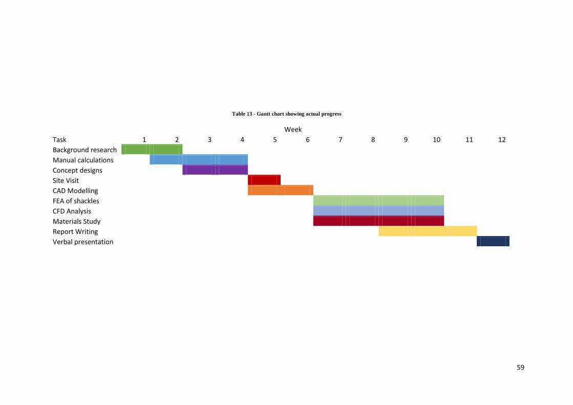
59
Table 13 - Gantt chart showing actual progress
Week
Task 1 2 3 4 5 6 7 8 9 10 11 12
Background research
Manual calculations
Concept designs
Site Visit
CAD Modelling
FEA of shackles
CFD Analysis
Materials Study
Report Writing
Verbal presentation
60
Figure 33 - Concept Design 1
Figure 34 - Concept Design 2

61
Figure 35 - Concept Design 3
Figure 36 - Concept Design 4
62
Figure 37 - Concept Design 5