Skew-Normal Variational Approximations for Bayesian InferenceBY J.T. ORMEROD1

School of Mathematics and Statistics, University of Sydney, Sydney 2006, Australia

10th of March, 2011

Abstract:

A new variational approximation based on multivariate skew-normal densities is developed.This paper overcomes most of the computational difficulties associated with the proposed ap-proximation and shows for several examples how the method can significantly improve uponaccuracy of the Laplace approximation, integrated nested Laplace approximation and Gaussianvariational approximations whilst being significantly faster than Markov chain Monte Carlomethods.

Key Words: Variational approximation; Skew-normal distribution; Laplace approximation; In-tegrated nested Laplace approximation; Machine learning; Markov chain Monte Carlo.

1 Introduction

In recent years there has been an increasing amount of research in approximate methods forBayesian inference. The driving force behind this research is the fact that while Monte Carlomethods can be made to be arbitrarily accurate they can be unacceptably slow when applied tolarge or complex problems. Approximate methods for Bayesian inference include Laplace-likemethods (Tierney & Kadane, 1986; Raudenbush, Yang & Yosef, 2000; Rue, Martino & Chopin,2009), several variational approximation approaches (Bishop, 2006; Ormerod & Wand, 2010;Wand et al., 2011) and expectation propagation (Minka, 2001). These methods can be quiteeffective when the posterior density is log-concave, or at least unimodal.

The Laplace-like approximations are perhaps the most pervasive analytic approximationsused in all of Statistics. Several variants exist in various contexts, including PQL (Breslow& Clayton, 1993), approximating ratios of integrals (Tierney & Kadane, 1986), higher orderLaplace approximations (Raudenbush et al., 2000) and, more recently, the integrated nestedLaplace approximation (INLA) of Rue et al. (2009). The Laplace approximation is elegant, easyto implement and highly efficient to compute. Unfortunately, if the posterior distribution is notsimilar in shape to a multivariate Gaussian the Laplace approximation may perform poorly inpractise.

The INLA method of Rue et al. (2009) deserves special attention. The INLA method isa specialized method for approximating Gaussian latent effect models. The key idea of thismethod is to use Laplace-like methods to integrate out Gaussian latent effects while using othernumerical methods to integrate out other parameters. A potential drawback of the method isthat it focuses on the calculation of marginal posterior densities, rather than the full posterior.If the underlying posterior distribution of the latent effects is approximately Gaussian then

1

INLA can be quite effective. However, when the underlying posterior distribution of the latenteffects is skewed INLA can perform poorly (for example see Fong, Rue & Wakefield, 2010).

Expectation propagation (EP) is another alternative to Monte Carlo methods and generallyoutperforms Laplace’s method in terms of accuracy (Kuss & Rasmussen, 2005). Some recentdevelopments by Opper & Winther (2005), Paquet, Winter & Opper (2009) and Cseke & Heskes(2010) provide further improvements in terms of accuracy. However, EP can be difficult toapply to some models and can suffer from convergence issues. For these reasons we will notpursue EP in this paper.

Variational approximations take a variety of forms (for an introduction see Bishop, 2006, orOrmerod & Wand, 2010). This type of approximation, related to mean-field approximations,includes variational Bayes, although such approximations can also be applied in frequentistsettings (see Hall, Ormerod & Wand, 2011a; Hall et al. 2011b; Ormerod & Wand, 2011). Thistype of approximation has been particularly successful when the model at hand is either suf-ficiently large and/or complex. Successful examples of these methods include document re-trieval (e.g. Jordan, 2004) and functional magnetic resonance imaging (e.g. Flandin & Penny,2007), cluster analysis for gene-expression data (Teschendorff et al., 2005) and finite mixturemodels (McGrory & Titterington, 2007).

In this paper we consider a particular type of parametric variational approximation, analternative to variations Bayes. A particular parametric variational approximation that hasrecently received some attention is the Gaussian variational approximation (GVA) where theposterior, like Laplace’s method, is approximated by a multivariate Gaussian density (Opper &Archambeau, 2009; Ormerod & Wand, 2011). This type of approximation, as one might expect,has similar properties to the Laplace approximation but empirically tends to outperform it interms of accuracy. However, like the Laplace approximation, the Gaussian variational approx-imation can perform poorly when the approximate posterior density is not similar in shape tothe multivariate Gaussian density.

The lack of flexibility of the Laplace and GVA methods leads to their failure when, for in-stance, the underlying posterior density is skewed. In this paper we develop skew-normalvariational approximations (SNVA) which seek to improve upon the Laplace and GVA meth-ods by employing a multivariate skew-normal density in order to make up for this potentialshortcoming. Although, many skew-normal distributions now exist (see Genton, 2004), we willuse the original multivariate skew-normal distributions proposed by Azzalini & Dalla Valle(1996). This extension makes particular sense when attempting to approximate log-concave, orat least unimodal, densities.

In utilizing the increased flexibility of the multivariate skew-normal density, over multi-variate Gaussian densities, the SNVA method can give substantial improvements over theLaplace’s or GVA methods. We illustrate and compare the SNVA method for examples in-cluding the normal sample, generalized linear models, generalized linear mixed models andan inhomogeneous noise model. In each of the examples the SNVA method gives better or atleast comparable accuracy to INLA for almost all parameters where a direct comparison is pos-sible. These examples also demonstrate two other advantages of SNVA over INLA, namely thefact that SNVA approximates the joint posterior distribution while INLA only approximatesmarginal posterior densities, and the fact that SNVA may be applied to models which INLAdoes not currently handle. The SNVA method is also reasonably fast.

2

The organization of the paper is as follows. Section 2 describes the basis for SNVA. Section3 describes how to calculate the SNVA lower bound on the log-likelihood. Section 4 describeshow we maximize this lower bound on the log-likelihood to improve the approximation. Sec-tion 5 demonstrates the advantages of the SNVA method for several Bayesian models andshows how for these examples the method requires at most univariate quadrature. Section 6provides some conclusions and discussion.

2 Skew-Normal Variational Approximations

Bayesian inference is mainly concerned with the calculation of the posterior density

p(θ|y) =p(y,θ)

p(y)(1)

where p(y) =∫

Θp(y,θ)dθ, the vector y denotes the observed response values, and θ denotes

all unobserved or hidden variables, for example model parameters, latent and auxiliary vari-ables or missing data, and Θ is the m-dimensional parameter space of θ. In this paper we willassume, for simplicity, that θ is continuous and that, unless otherwise specified, the domain ofintegration used in integrals is Θ. Unfortunately, the direct calculation of the quantity p(θ|y) isonly possible for special cases and approximation is required.

Most variational approximations are based on minimizing the Kullback-Leibler (KL) dis-tance between a density q(θ) and p(θ|y) given by

KL(q(θ), p(θ|y)) =

∫q(θ) log

{q(θ)

p(θ|y)

}dθ (2)

noting that the Kullback-Leibler distance is positive and zero if and only if q(θ) = p(θ|y) almosteverywhere (Kullback & Leibler, 1951).

Parametric variational approximations attempt to minimize (2) subject to the restriction

q(θ) = q(θ; ξ)

where q(θ; ξ) is some conveniently chosen parametric density and ξ are parameters of thatdensity (called variational parameters). Using simple algebraic manipulations it is easy to show

log p(y) =

∫p(y,θ)dθ (3)

=

∫q(θ; ξ) log

{p(y,θ)

q(θ; ξ)

}dθ +

∫q(θ; ξ) log

{q(θ; ξ)

p(θ|y)

}dθ (4)

=

∫q(θ; ξ) log

{p(y,θ)

q(θ; ξ)

}dθ + KL(q(θ), p(θ|y)) (5)

≥∫q(θ; ξ) log p(y,θ)dθ −

∫q(θ; ξ) log q(θ; ξ)dθ (6)

=

∫q(θ; ξ) log p(y,θ)dθ + Eq(ξ) (7)

≡ log pq(y; ξ) (8)

3

which follows from the fact that the KL-divergence, the second term on the right hand side of(4), is positive. We can also see from (4)–(8) that log p(y) − log pq(y; ξ) = KL(q(θ; ξ), p(θ|y)) sothat maximizing pq(y; ξ) with respect to ξ is equivalent to minimizing KL(q(θ; ξ), p(θ|y)) withrespect to ξ. Furthermore, in order to calculate the lower bound for a particular q(θ; ξ) we needto be able to calculate Eq(ξ) = −

∫q(θ; ξ) log q(θ; ξ)dθ, the (Shannon’s) entropy of q(θ; ξ).

As was motivated in the introduction we choose q to be the multivariate skew-normal den-sity originally proposed by Azzalini & Dalla Valle (1996). We will say a m-dimensional ran-dom vector θ has a multivariate skew-normal distribution with skewness vector d, denotedθ ∼ SN(µ,Λ,d), if its probability density function is given by

q(θ; µ,Λ,d) = 2φΛ(θ − µ)Φ(dT (θ − µ)) (9)

where θ ∈ Θ = Rm, φΛ(θ − µ) denotes the multivariate Gaussian density with mean vectorµ and covariance matrix Λ, Φ denotes the cumulative distribution function for the standardunivariate Gaussian distribution with µ, Λ and d being the location, scale and skewness pa-rameters respectively. Note that µ and d are unrestricted in Rm while Λ must be positivedefinite. It is easy to see that when d = 0 the multivariate Gaussian density is recovered.

We call the parametric variational approximations where q is given by (9) a skew-normalvariational approximation (SNVA). For this q the variational parameters are ξ = (µ,Λ,d). TheGaussian variational approximation (GVA) is the special case when d = 0 denoted pG(y; µ,Λ).Note that the SNVA is guaranteed to be a better approximation of the marginal likelihood thanGVA in the sense that pSN is a tighter lower bound on p(y) than pG since

p(y) ≥ supµ,Λ,d

{pSN(y; µ,Λ,d)} ≥ supµ,Λ,d

{pSN(y; µ,Λ,d) such that d = 0} = supµ,Λ{pG(y; µ,Λ)} .

We will now focus on the calculation of pSN.

3 Calculating the Variational Lower Bound

The calculation of pSN requires applying various properties of the skew normal density (9). Wewill briefly review only the most pertinent of these to show some new results required by theskew-normal variational approximation. These results will also be useful for calculating thelower bound pSN and its derivatives for the examples considered later on.

The moment generating function of q is given by M(t) = E(exp(tTθ)) = 2 exp(µT t +12tTΛt)Φ(δT t) where δ = Λd/(1 + dTΛd)1/2 which we can use to show that E(θ) = µ +

√2/πδ

and Cov(θ) = Λ − (2/π)δδT . Furthermore, we can use the moment generating function(Gonzalex-Farıas, Domınguez-Molina & Gupta, 2004) or alternatively (Azzalini & Capitanio,1999) to show that the skew-normal distribution is closed under linear transformations, i.e. forany m× r matrix A (of rank r) and r × 1 vector b we have

z = Aθ + b ∼ SN(µz,Λz,dz) (10)

where µz = Aµ + b, Λz = AΛAT and dz = Λ−1z AΛd(1 + dTΛ(I − ATΛ−1

z AΛ)d)−1/2. Usingthis expression it is easy to show that the “δ” corresponding to this transformation is given by

4

δz = Aδ. From the closure of skew-normal densities under linear transformations it is easy toshow that the skew-normal distribution is also closed under marginalization, i.e. by setting Ato eTi in (10) where ei is the zero vector except the value 1 in the ith element. Finally, using theclosure under linear transformations property, we have∫

Rmq(θ; µ,Λ,d)f(Aθ + b))dθ = E [f(Aθ + b)] = E [f(z)] =

∫Rrq(z; µz,Λz,dz)f(z)dz (11)

which, provided r < m, reduces the dimensionality of the integral to be calculated. This fact isused to derive the following new result.

Result 1 – Entropy Expression: The entropy function of 2φΛ(θ − µ)Φ(dT (θ − µ)) is given by

E(µ,Λ,d) = −∫q(θ; µ,Λ,d) log q(θ; µ,Λ,d)dθ = 1

2log |2eπΛ| − log(2)−Ψ(dTΛd) (12)

where Ψ(σ2) =∫

R 2φσ(z)Φ(z) log Φ(z)dz.

Proof: See Appendix A.1.

The properties and the calculation of Ψ and its derivatives are discussed in Appendix A.1. Tothe best of the author’s knowledge the entropy expression for the skew-normal distributionhas not been previously derived.

Using the expression for the entropy of the skew-normal density (12) with (5) the skew-normal variational approximation the log of the marginal likelihood may be written as

log pSN(y; µ,Λ,d) = 12

log |2πΛ|+ m2− log(2)−Ψ(dTΛd) + fSN(µ,Λ,d)

where fSN(µ,Λ,d) =

∫2φΛ(θ − µ)Φ(dT (θ − µ)) log p(y,θ)dθ.

(13)

Many of the above expectations can be calculated using the moment generating functionand linear transformations results above. Calculation of the expectations in two of the exam-ples in Section 5 will be aided by the following result:

Result 2: Suppose that q(θ; µ,Λ,d) = 2φΛ(θ − µ)Φ(dT (θ − µ)) then

exp(tTθ)q(θ; µ,Λ,d) = 2 exp(tTµ + tTΛt/2)Φ(δT t)q(θ; µ,Λ,d, t) (14)

where q(θ; µ,Λ,d, t) =Φ(dT (θ − µ))

Φ(δT t)φΛ(θ − µ−Λt). (15)

Note that q(θ; µ,Λ,d, t) is a special case of the multivariate skew-normal distribution first pro-posed by Arnold & Beaver (2002) and when t = 0 the skew-normal distribution of Azzalini &Dalla Valle (1996) is obtained. Let θ be a random variable whose density is (15). Then is canbe shown that the moment generating function of θ is given by M(s) = 2 exp(sT (µ + Λt) +

sTΛs/2)Φ(δT (s+t))/Φ(δT t) and hence E(θ) = µ+Λt+ ζ1(δT t)δ and Cov(θ) = Λ+ ζ2(δT t)δδT

where ζk(x) = dk log Φ(x)/dxk. Note that special care needs to be taken to calculate ζk(x) whenx is large and negative for k ≥ 1. A robust implementation of ζk(x) is given in the R packagesn (Azzalini, 2010).

5

4 Maximising the Variational Lower Bound

We now address the problem of maximizing pSN(y; µ,Λ,d) with respect to the variational pa-rameters (µ,Λ,d). Many efficient numerical optimization methods only require gradient infor-mation to perform this optimization (Nocedal & Wright, 1999; Luenberger & Ye, 2008). Quasi-Newton methods approximate the Hessian by using differences of successive iterations of thegradient vector. A particularly popular quasi-Newton method is the BFGS method, named af-ter its inventors Broyden, Fletcher, Goldfarb and Shanno. This method is implemented in the Rfunction optim(). In order to use this method we will need the expressions for the derivativesof pSN(y; µ,Λ,d) with respect to the variational parameters (µ,Λ,d).

4.1 Derivative Expressions

There are a number of ways to parametrize Λ. Suppose that, for the time being, that vech(Λ) arethe unique parameters of Λ. Suppose that the 1×d derivative vector of a function f(x), denotedDxf(x), is the vector with ith entry ∂f(x)/∂xi and the corresponding Hessian matrix is denotedby Hxf(x) = Dx{Dxf(x)}T . Also, to simplify upcoming expressions let f(θ) = log p(y,θ),g(θ) = Dθ log p(y,θ) and H(θ) = Hθ log p(y,θ). Then the expressions for the derivatives of pSN

with respect to (µ,vech(Λ),d) are given in the following result.

Result 3 – Derivative Expressions: Assuming that log p(y,θ) is twice differentiable with respect toθ the derivatives of log pSN ≡ log pSN(y; µ,Λ,d) are given by

Dµ log pSN = gSN

Dd log pSN = c1(Λ− δδT )gG −Ψ′(dTΛd)Λdd log pSN

dΛij

= 12

[Λ−1 + HSN + c1(gGdT + dgTG )− c2ddT

]ij

(16)

where c1 =√

2/π/√

1 + dTΛd, c2 = Ψ′(dTΛd) + c1dTΛgG/(1 + dTΛd),

gSN ≡ gSN(µ,Λ,d) =

∫Rm

2φΛ(θ − µ)Φ(dT (θ − µ))g(θ)dθ

HSN ≡ HSN(µ,Λ,d) =

∫Rm

2φΛ(θ − µ)Φ(dT (θ − µ))H(θ)dθ

and gG ≡ gSN(µ,Λ− δδT ,0).

Proof: See Appendix A.2.

The evaluation of Dµ log pSN, Dd log pSN and Dvech(Λ) log pSN would require different results, forexample, if p(y,θ) included Laplace distributed or other non-differentiable components.

A significant concern when we attempt to maximize pSN is ensuring Λ remains positivedefinite. This constraint can be ensured by using the parameterization Λ(r) = RTR where R isan upper triangular matrix with erii on the diagonal and rij in the upper right elements of thematrix. In this case the derivatives with respect to the rijs are given by

∂ log pSN

∂rij=[R−T + R

(HSN + c1(gGdT + dgTG )− c2ddT

)]ijerijI(i=j), 1 ≤ i ≤ m, i ≤ j ≤ m

6

where I(·) is the indicator function taking the value 1 if the condition is true and 0 otherwiseand the terms appearing are defined in the derivative expression results above.

4.2 Initial Values

Note that Result 3 coincides with the results obtained by Opper & Archambeau (2009) for GVA,i.e. when d = 0. We can also see, based on this observation, that if (µ∗G,Λ

∗G) maximizes pG then

(µ∗G,Λ∗G,0) is at least a local maximiser of pSN. Later we will see examples where (µ∗G,Λ

∗G,0) is

neither the only maximiser nor the global maximiser of pSN.We will use the Laplace approximation to provide ballpark starting values for SNVA. As-

suming that the joint distribution p(y,θ) is twice differentiable and Θ = Rm then Laplace’smethod approximates the posterior density p(θ|y) by qL(θ) = N(µ,Λ) where µ is the maximiserof p(y,θ) and Λ = [−H(µ)]−1. These values can be found quickly an easily by applying New-ton’s method whose updates are given by Λ(t+1) ←

[−H(µ(t))

]and µ(t+1) ← µ(t)+Λ(t+1)g(µ(t)).

Upon convergence µ and Λ take the values µ(t) and Λ(t) respectively. Given these values theLaplace approximation to the marginal likelihood is pL(y) = |2πΛ|1/2p(y,µ).

5 Illustrations

In this section we demonstrate the value of the SNVA method. We will compare various ap-proximations with an accurate MCMC approximation which we will use as a “gold standard”.To this end, for each of models fitted in this paper, we will generate a long run of MCMC sam-ples using the R package BRugs (Ligges et al., 2009). Unless otherwise specified in the followingexamples we will generate 5× 104 burn-in samples followed by a further 5× 106 samples usinga thinning factor of 5 so that a total of 106 samples are available for inference. Furthermore, wewill use the over-relaxed form of MCMC as described by Neal (1998) to improve mixing. InBRugs this involves setting the option overRelax=TRUE when calling the modelUpdate()function . Kernel density estimates qMCMC(θi) of the p(θi|y)s were then constructed using the 106

MCMC samples. These We should expect these Kernel density estimates to be nearly perfectposterior density approximations.

Let the vector θi denote a generic model parameter of length at most two. There are variousways to measure the accuracy between an approximate posterior density q(θi) and a “goldstandard” qGS(θi). We will compare various posterior density estimates and use the L1-norm orIntegrated Absolute Error (IAE) defined by

IAE(q) =

∫|q(θi)− qGS(θi)|dθi

where for the purposes of this paper we will use the MCMC approximation described aboveas the “gold standard”, i.e. qGS(θi) = qMCMC(θi). This error measure has the advantages ofbeing invariant to monotone transformations of the parameter θ and is a scale independentnumber between 0 and 2 (e.g. Devroye & Gyorfi, 1985). This motivates the following measureof accuracy

Accuracy(q(θi)) = 1− 12IAE(q(θi))

7

noting that 0 ≤ Accuracy(q(θi)) ≤ 1 and will be expressed as a percentage. We will restrict θito be at most two-dimensional so that IAE(θi) can be approximated numerically using one ortwo-dimensional quadrature.

We could also use some alternative measures of accuracy. Other measures such as the KL-divergence between q(θ|y) and p(θ|y) is computationally both more demanding and delicatedue to the fact that this requires the calculation of the marginal likelihood. We might also betempted to use the KL-divergence between marginal posterior densities. However, as noted byHall (1987), this measure is dominated by the tail behavior of q(θ) and qMCMC(θ).

Using the above measure of accuracy we will compare the Laplace, INLA, GVA and SNVAmethods for the normal sample model (Example 1), generalized linear models (Example 2),generalized linear mixed models (Example 3) and linear regression with inhomogeneous noise(Example 4). In Ormerod & Wand (2010) the variational Bayes (VB) approach was describedfor Example 1 and so for this example we will also compare VB. Note that for the INLA methodwe use the R package INLA (available from http://www.r-inla.org/) and use all defaultoptions except that the option control.inla=list(strategy="FIT SCGAUSSIAN")wasused as the option which is expected to give the best accuracy.

5.1 Example 1 – Normal Sample

A good place to start is to consider one of the simplest Bayesian models for which integration isrequired, the estimation of a normal sample. It is by no means a difficult problem, since MCMCtakes negligible time to fit, however this simple example serves to illustrate the differences invarious approximation methods.

Consider the modelyi|µ, σ2 ∼ N(µ, σ2), 1 ≤ i ≤ n, (17)

with priors µ ∼ N(0, σ2µ) and σ2 ∼ IG(a, b).

The marginal likelihood may be written as p(y) =∫∞

0

∫∞−∞ p(y, µ, σ

2)dµdσ2 where p(y, µ, σ2)

may be written as p(y, µ, σ2) = exp{−(A+n/2+1) log(σ2)−σ−2(B+‖y−µ1‖2/2)−µ2/(2σ2µ)+κ}

where the sum of the constant terms, κ, is given by κ = − log(2π) − log(σ2µ)/2 − A log(B) −

log Γ(A). In order to transform the domain of the integral to R2, so that we can use SNVA, weuse the transformation σ2 = eγ . Based on Theorem 2.1.5 of Casella & Berger (2002) the prior forγ becomes p(γ) = AB exp(−Aγ − Be−γ)/Γ(γ). Let θ = (µ, γ) so that the joint likelihood may bewritten as p(y,θ) = exp{− (A+ n/2) γ − e−γ (B + ‖y − µ1‖2/2)− µ2/(2σ2

µ) + κ}.Next, consider the partitions

µ =

[µµµγ

], δ =

[δµδγ

]and Λ =

[Λµµ Λµγ

Λγµ Λγγ

]of µ, δ and Λ respectively, corresponding to the elements of θ. Note that we will be usingsimilar partitions of µ, δ and Λ in later problems.

8

Then, using the results in Section 3, we can show that expressions for fSN, gSN and HSN are

fSN = −(A+ n

2

)(µγ +

√2πδγ

)−M

(B + 1

2T)− 1

2σ2µ

(µ2µ + 2

√2πµµδµ + Λµµ

)gSN =

[M1Tn (y − µ1n)− (µµ +

√2πδµ)/σ2

µ

M(B + 1

2T)−(A+ n

2

) ]and HSN = −

[Mn+ σ−2

µ M1Tn (y − µ1n)M1Tn (y − µ1n) M

(B + 1

2T) ]

respectively where M = 2e−µγ+Λγγ/2Φ(−δγ), T = ‖y − µ1n‖2 + n(Λµµ + ζ2(−δγ)δ2µ) and µ =

µµ − Λγµ + ζ1(−δγ)δµ.To test each approximation we simulated data from (17) with sample size n = 6 and true

parameters ν = 6 and σ2 = 225. We used the hyperparameters σ2µ = 104 and A = B = 0.01. For

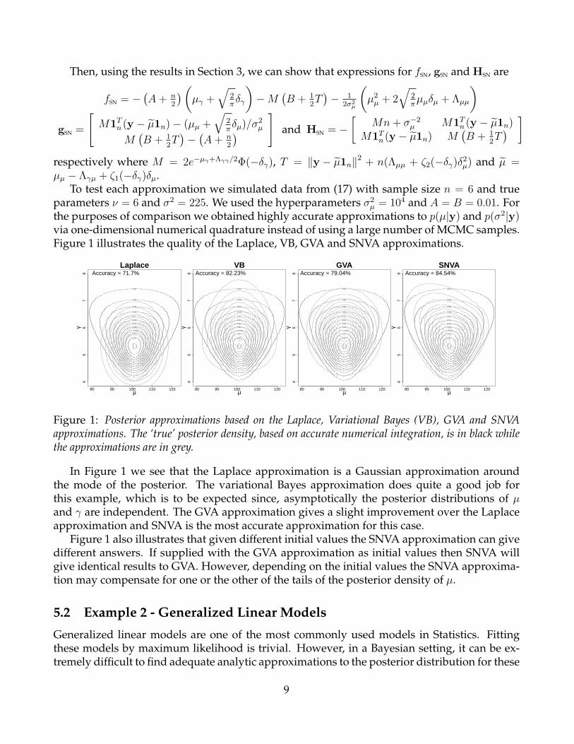
the purposes of comparison we obtained highly accurate approximations to p(µ|y) and p(σ2|y)via one-dimensional numerical quadrature instead of using a large number of MCMC samples.Figure 1 illustrates the quality of the Laplace, VB, GVA and SNVA approximations.

Laplace

µ

γ

0.002

0.004

0.006

0.008

0.01

0.012

0.014

0.016

0.018

0.02

0.022

80 90 100 110 120

45

67

8

0.002

0.004

0.006

0.008

0.01

0.012

0.014

0.016

0.018

0.02

0.022

0.024

0.026

Accuracy = 71.7%VB

µ

γ

0.002

0.004

0.006

0.008

0.01

0.012

0.014

0.016

0.018

0.02

0.022

80 90 100 110 120

45

67

8

0.002

0.004

0.006

0.008

0.01

0.012

0.014

0.016

0.018

0.02

0.022

0.024

0.026

Accuracy = 82.23%GVA

µ

γ 0.002

0.004

0.006

0.008

0.01

0.012

0.014

0.016

0.018

0.02

0.022

80 90 100 110 120

45

67

8

0.002

0.004

0.006

0.008

0.01

0.012

0.014

0.016

0.018

0.02

0.022

0.024

0.026

Accuracy = 79.04%SNVA

µγ

0.002

0.004

0.006

0.008

0.01

0.012

0.014

0.016

0.018

0.02

0.022

80 90 100 110 120

45

67

8

0.002

0.004

0.006

0.008

0.01

0.012

0.014

0.016

0.018

0.02

0.022

Accuracy = 84.54%

Figure 1: Posterior approximations based on the Laplace, Variational Bayes (VB), GVA and SNVAapproximations. The ‘true’ posterior density, based on accurate numerical integration, is in black whilethe approximations are in grey.

In Figure 1 we see that the Laplace approximation is a Gaussian approximation aroundthe mode of the posterior. The variational Bayes approximation does quite a good job forthis example, which is to be expected since, asymptotically the posterior distributions of µand γ are independent. The GVA approximation gives a slight improvement over the Laplaceapproximation and SNVA is the most accurate approximation for this case.

Figure 1 also illustrates that given different initial values the SNVA approximation can givedifferent answers. If supplied with the GVA approximation as initial values then SNVA willgive identical results to GVA. However, depending on the initial values the SNVA approxima-tion may compensate for one or the other of the tails of the posterior density of µ.

5.2 Example 2 - Generalized Linear Models

Generalized linear models are one of the most commonly used models in Statistics. Fittingthese models by maximum likelihood is trivial. However, in a Bayesian setting, it can be ex-tremely difficult to find adequate analytic approximations to the posterior distribution for these

9

models. Furthermore, Bayesian generalized linear models closely share many of the compu-tational difficulties with generalized linear mixed models, an active area of research, and arethus worthy of consideration.

Consider the model y|β ∼ Poisson(exp(Xβ)) or y|β ∼ Binomial(expit(Xβ)) where expit(x) =ex/(1 + ex). We employ the prior β ∼ N(0,Σ) so that the joint likelihood may be written asp(y,β) ∝ exp

{yTXβ − 1T b(Xβ)− 1

2βTΣ−1β

}where b(x) = ex for the Poisson model and

b(x) = log(1 + ex) for the logistic model. The functions fSN, gSN and HSN are given by

fSN = yTX(µ +√

2πδ)− 1TnB

(0)(Xµ,dg(XΛXT ),Xδ)− 12µTΣ−1µ−

√2πµTΣ−1δ − 1

2tr[Σ−1Λ

]gSN = XT (y −B(1)(Xµ,dg(XΛXT ),Xδ))−Σ−1(µ +

√2πδ)

HSN = −XTdiag(B(2)(Xµ,dg(XΛXT ),Xδ))X−Σ−1

where B(r)(µ, σ2, δ) =∫∞−∞ 2φσ(x− µ)Φ(d(x− µ))b(x)dx with d = (δ/σ)/

√1− δ2/σ2 and dg(A)

is the vector obtained from taking the diagonal elements of a square matrix A. For the Pois-son model the function B(r)(µ, σ2, δ) is available analytically and is given by B(r)(µ, σ2, δ) =2 exp

{µ+ 1

2σ2}

Φ(δ) whereas for the logistic model univariate numerical quadrature is required.The adaptive Gauss-Hermite quadrature method described by Liu & Pierce (1994) or Pinheiro& Bates (1995) is a particularly suitable for this type of integral.

5.2.1 O-ring Data

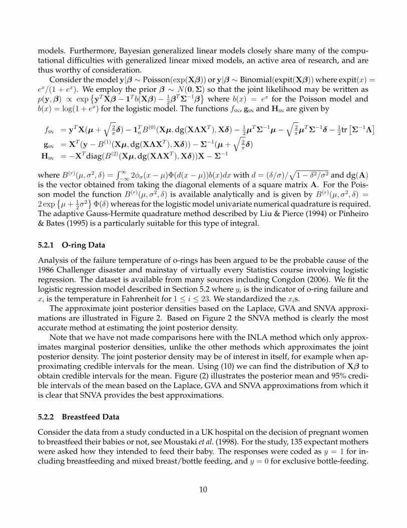
Analysis of the failure temperature of o-rings has been argued to be the probable cause of the1986 Challenger disaster and mainstay of virtually every Statistics course involving logisticregression. The dataset is available from many sources including Congdon (2006). We fit thelogistic regression model described in Section 5.2 where yi is the indicator of o-ring failure andxi is the temperature in Fahrenheit for 1 ≤ i ≤ 23. We standardized the xis.

The approximate joint posterior densities based on the Laplace, GVA and SNVA approxi-mations are illustrated in Figure 2. Based on Figure 2 the SNVA method is clearly the mostaccurate method at estimating the joint posterior density.

Note that we have not made comparisons here with the INLA method which only approx-imates marginal posterior densities, unlike the other methods which approximates the jointposterior density. The joint posterior density may be of interest in itself, for example when ap-proximating credible intervals for the mean. Using (10) we can find the distribution of Xβ toobtain credible intervals for the mean. Figure (2) illustrates the posterior mean and 95% credi-ble intervals of the mean based on the Laplace, GVA and SNVA approximations from which itis clear that SNVA provides the best approximations.

5.2.2 Breastfeed Data

Consider the data from a study conducted in a UK hospital on the decision of pregnant womento breastfeed their babies or not, see Moustaki et al. (1998). For the study, 135 expectant motherswere asked how they intended to feed their baby. The responses were coded as y = 1 for in-cluding breastfeeding and mixed breast/bottle feeding, and y = 0 for exclusive bottle-feeding.

10

Laplace

β0

β 1 0.2

0.4

0.6

0.8

1

1.2

1.4

1.6

1.8

2

2.2

−3.0 −2.5 −2.0 −1.5 −1.0 −0.5 0.0

−0.

6−

0.4

−0.

20.

0

0.2

0.4

0.6

0.8

1

1.2

1.4

1.6

1.8

2

2.2

2.4

2.6

Accuracy=83.72

GVA

β0

β 1

0.2

0.4

0.6

0.8

1

1.2

1.4

1.6

1.8

2

2.2

−3.0 −2.5 −2.0 −1.5 −1.0 −0.5 0.0

−0.

6−

0.4

−0.

20.

0

0.2

0.4

0.6

0.8

1

1.2

1.4

1.6

1.8

2

2.2

2.4

Accuracy=84.94

SNVA

β0

β 1

0.2

0.4

0.6

0.8

1

1.2

1.4

1.6

1.8

2

2.2

−3.0 −2.5 −2.0 −1.5 −1.0 −0.5 0.0

−0.

6−

0.4

−0.

20.

0

0.2

0.4

0.6

0.8

1

1.2

1.4

1.6

1.8

2

2.2

Accuracy=94.95

55 60 65 70 75 80

0.0

0.2

0.4

0.6

0.8

1.0

Laplace

x

P(f

ailu

re)

55 60 65 70 75 80

0.0

0.2

0.4

0.6

0.8

1.0

GVA

x

P(f

ailu

re)

55 60 65 70 75 80

0.0

0.2

0.4

0.6

0.8

1.0

SNVA

x

P(f

ailu

re)

Figure 2: [Top panels] Illustrations of the Laplace, GVA and SNVA approximations (gray) of the jointposterior density for logistic regression model applied to the o-ring dataset along with the “exact” poste-rior based on bivariate numerical integration (black). [Bottom panels] Illustrations of the Laplace, GVAand SNVA approximations (gray) of the posterior mean and 95% credible intervals of the mean for logis-tic regression model applied to the o-ring dataset along with these “exact” quantities based on MCMCsimulations (black).

Available covariates included the advancement of the pregnancy (end pregnancy = 1 or begin-ning pregnancy = 0), how the mothers were fed as babies (howfed), how the mother’s friendfed their babies (howfedfr), whether they had a partner (partner), the mother’s age (age),the age at which they left full-time education (educat), their ethnic group (ethnic) and ifthey have ever smoked (smokebf) or if they had stopped smoking (smokenow). The data hasalso been analysed by and is available from the website of the book by Heritier et al. (2009).

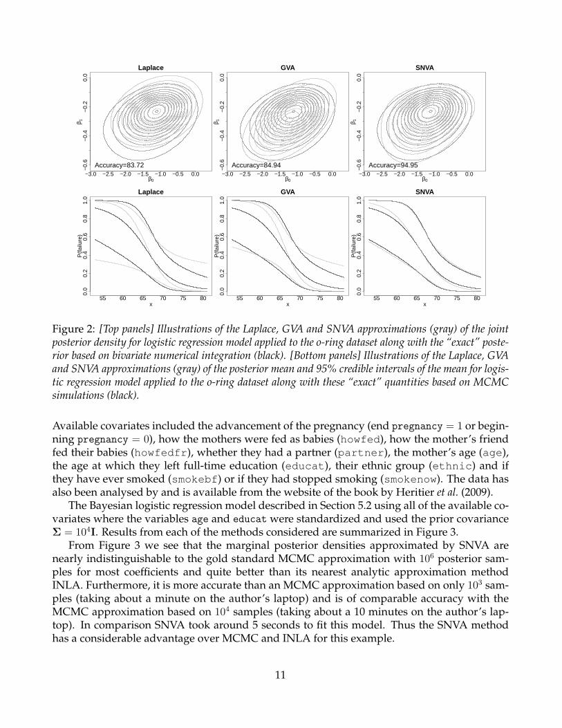
The Bayesian logistic regression model described in Section 5.2 using all of the available co-variates where the variables age and educat were standardized and used the prior covarianceΣ = 104I. Results from each of the methods considered are summarized in Figure 3.

From Figure 3 we see that the marginal posterior densities approximated by SNVA arenearly indistinguishable to the gold standard MCMC approximation with 106 posterior sam-ples for most coefficients and quite better than its nearest analytic approximation methodINLA. Furthermore, it is more accurate than an MCMC approximation based on only 103 sam-ples (taking about a minute on the author’s laptop) and is of comparable accuracy with theMCMC approximation based on 104 samples (taking about a 10 minutes on the author’s lap-top). In comparison SNVA took around 5 seconds to fit this model. Thus the SNVA methodhas a considerable advantage over MCMC and INLA for this example.

11

−2 −1 0 1 2 3 4 5

0.0

0.1

0.2

0.3

0.4 intercept

appr

ox. p

oste

rior

0 1 2 3

0.0

0.2

0.4

0.6

howfedfr

appr

ox. p

oste

rior

−5 −4 −3 −2 −1 0

0.0

0.1

0.2

0.3

0.4

0.5

ethnic

appr

ox. p

oste

rior

−0.5 0.0 0.5 1.0 1.5 2.0

0.0

0.2

0.4

0.6

0.8

1.0

educat

appr

ox. p

oste

rior

−0.5 0.0 0.5 1.0

0.0

0.4

0.8

1.2

age

appr

ox. p

oste

rior

−3 −2 −1 0

0.0

0.2

0.4

0.6

pregnancyap

prox

. pos

terio

r

−1 0 1 2

0.0

0.2

0.4

0.6

howfed

appr

ox. p

oste

rior

−1 0 1 2 3

0.0

0.1

0.2

0.3

0.4

0.5

partner

appr

ox. p

oste

rior

−8 −6 −4 −2

0.0

0.1

0.2

0.3

0.4

smokenow

appr

ox. p

oste

rior

−1 0 1 2 3 4 5 6

0.0

0.1

0.2

0.3

0.4

smokebf

appr

ox. p

oste

rior MCMC

SNVA

INLA

●

●

●

Laplace GVA INLA SNVA MC3 MC4

8590

9510

0 Breastfeed Data Accuracies

Figure 3: The left panel illustrates the posterior approximations based on MCMC (106 samples), SNVAand INLA approximations for the logistic regression model for the breastfeed dataset. The right panel isa boxplot of the accuracies for the Laplace, GVA, SNVA, INLA and MCMC methods with 103 samples(MC3) and 104 samples (MC4).

5.2.3 Simulated Data

We first compare the Laplace approximation, GVA, INLA and SNVA approximations for sim-ulated data. For large n the posterior distribution becomes increasingly Gaussian. Thus, forsufficiently large n each of these methods will perform similarly well.

We have chosen the following simulation settings so that n is small relative to m so as toinduce the more difficult case where the posterior distribution can become quite skewed: m ∈(4, 8, 16, 20, 30, 40), β = (2,−2, . . . , 2,−2)/m, xij ∼ N(0, 1), 1 ≤ i ≤ m, 1 ≤ i ≤ n with the priorcovariance Σ = 104I. We set n = 3m/2 for the Poisson case and n = 2m for the logistic case.Also, in order to avoid pathological cases, we discarded simulations where the R function glmfailed to converge or the number of zeros was greater than m− 1 for the Poisson case or whereeither the number of successes or failures was less than 2. Lastly, for the purposes of simulation,we used results based on 104 MCMC samples (instead of 106) as the gold standard to reducethe total time of running these simulations. We compared the accuracies for 50 simulated datawith the above settings and the results are summarized in Figure 4.

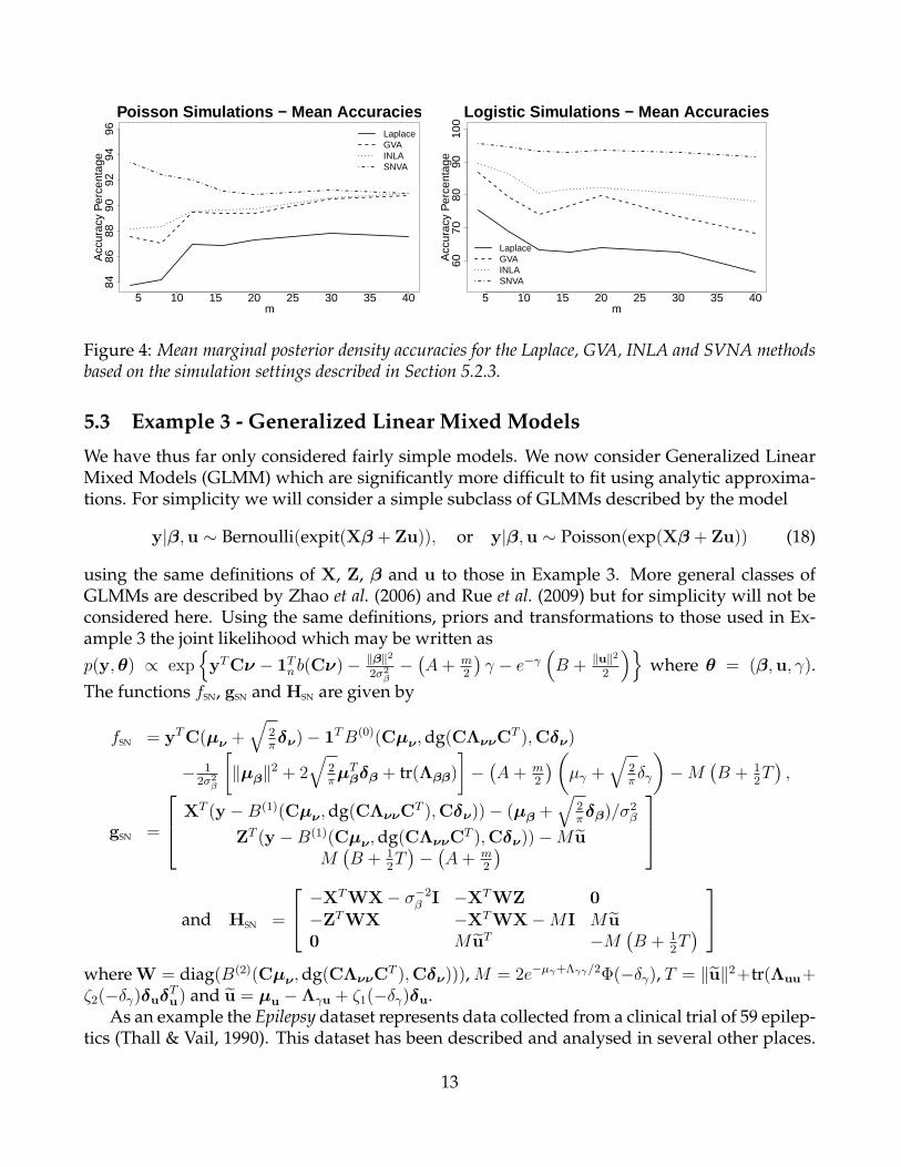
From Figure 4 we can see that SNVA performs better than the other methods for all settingsfor both the Poisson case and the logistic case. However, for the Poisson case, the relative ad-vantage of SNVA over GVA and INLA seems to diminish for largerm. This is perhaps because,for larger m, the sample size n is relatively large and the posterior density is reasonably Gaus-sian. Unfortunately this increased accuracy comes at a price. For the logistic case, althoughsuch a comparison is not completely fair, our implementation of SNVA was roughly 10 timesslower than INLA.

12

5 10 15 20 25 30 35 40

8486

8890

9294

96Poisson Simulations − Mean Accuracies

m

Acc

urac

y P

erce

ntag

e

LaplaceGVAINLASNVA

5 10 15 20 25 30 35 40

6070

8090

100

Logistic Simulations − Mean Accuracies

m

Acc

urac

y P

erce

ntag

e

LaplaceGVAINLASNVA

Figure 4: Mean marginal posterior density accuracies for the Laplace, GVA, INLA and SVNA methodsbased on the simulation settings described in Section 5.2.3.

5.3 Example 3 - Generalized Linear Mixed Models

We have thus far only considered fairly simple models. We now consider Generalized LinearMixed Models (GLMM) which are significantly more difficult to fit using analytic approxima-tions. For simplicity we will consider a simple subclass of GLMMs described by the model

y|β,u ∼ Bernoulli(expit(Xβ + Zu)), or y|β,u ∼ Poisson(exp(Xβ + Zu)) (18)

using the same definitions of X, Z, β and u to those in Example 3. More general classes ofGLMMs are described by Zhao et al. (2006) and Rue et al. (2009) but for simplicity will not beconsidered here. Using the same definitions, priors and transformations to those used in Ex-ample 3 the joint likelihood which may be written asp(y,θ) ∝ exp

{yTCν − 1Tnb(Cν)− ‖β‖

2

2σ2β−(A+ m

2

)γ − e−γ

(B + ‖u‖2

2

)}where θ = (β,u, γ).

The functions fSN, gSN and HSN are given by

fSN = yTC(µν +√

2πδν)− 1TB(0)(Cµν ,dg(CΛννCT ),Cδν)

− 12σ2β

[‖µβ‖2 + 2

√2πµT

βδβ + tr(Λββ)

]−(A+ m

2

)(µγ +

√2πδγ

)−M

(B + 1

2T),

gSN =

XT (y −B(1)(Cµν ,dg(CΛννCT ),Cδν))− (µβ +√

2πδβ)/σ2

β

ZT (y −B(1)(Cµν ,dg(CΛννCT ),Cδν))−M uM(B + 1

2T)−(A+ m

2

)

and HSN =

−XTWX− σ−2β I −XTWZ 0

−ZTWX −XTWX−MI M u0 M uT −M

(B + 1

2T)

where W = diag(B(2)(Cµν ,dg(CΛννCT ),Cδν))),M = 2e−µγ+Λγγ/2Φ(−δγ), T = ‖u‖2+tr(Λuu+ζ2(−δγ)δuδTu) and u = µu −Λγu + ζ1(−δγ)δu.

As an example the Epilepsy dataset represents data collected from a clinical trial of 59 epilep-tics (Thall & Vail, 1990). This dataset has been described and analysed in several other places.

13

The reader may refer to Thall & Vail (1990), Breslow & Clayton (1993), Rue et al.(2009) orOrmerod & Wand (2011) for a full description. We will consider the Poisson random inter-cept model

yij|β, ui ∼ Poisson[exp{β0 + ui + βvisit visitj + βbase log(basei/4)

+βtrt trti + βbaseXtrt log(basei/4)× trti + βage log(agei)}]

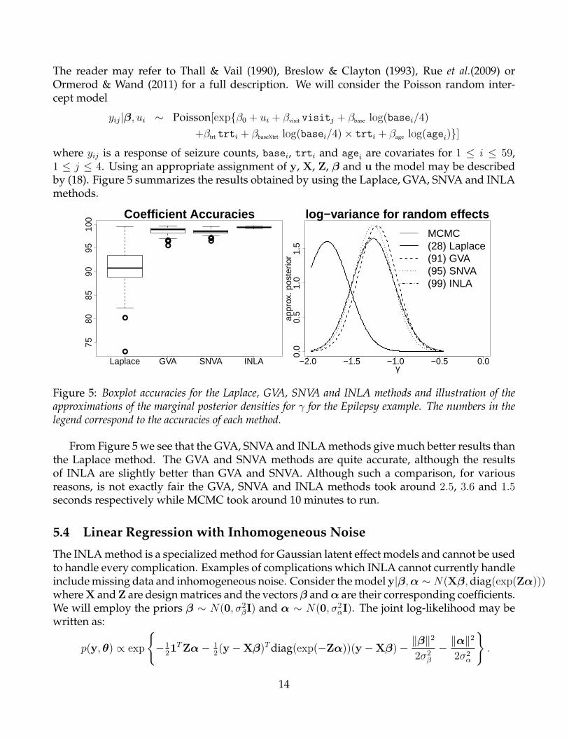
where yij is a response of seizure counts, basei, trti and agei are covariates for 1 ≤ i ≤ 59,1 ≤ j ≤ 4. Using an appropriate assignment of y, X, Z, β and u the model may be describedby (18). Figure 5 summarizes the results obtained by using the Laplace, GVA, SNVA and INLAmethods.

●

●

●●●●

●●●●

Laplace GVA SNVA INLA

7580

8590

9510

0 Coefficient Accuracies

−2.0 −1.5 −1.0 −0.5 0.0

0.0

0.5

1.0

1.5

log−variance for random effects

γ

appr

ox. p

oste

rior

MCMC(28) Laplace(91) GVA(95) SNVA(99) INLA

Figure 5: Boxplot accuracies for the Laplace, GVA, SNVA and INLA methods and illustration of theapproximations of the marginal posterior densities for γ for the Epilepsy example. The numbers in thelegend correspond to the accuracies of each method.

From Figure 5 we see that the GVA, SNVA and INLA methods give much better results thanthe Laplace method. The GVA and SNVA methods are quite accurate, although the resultsof INLA are slightly better than GVA and SNVA. Although such a comparison, for variousreasons, is not exactly fair the GVA, SNVA and INLA methods took around 2.5, 3.6 and 1.5seconds respectively while MCMC took around 10 minutes to run.

5.4 Linear Regression with Inhomogeneous Noise

The INLA method is a specialized method for Gaussian latent effect models and cannot be usedto handle every complication. Examples of complications which INLA cannot currently handleinclude missing data and inhomogeneous noise. Consider the model y|β,α ∼ N(Xβ,diag(exp(Zα)))where X and Z are design matrices and the vectors β and α are their corresponding coefficients.We will employ the priors β ∼ N(0, σ2

βI) and α ∼ N(0, σ2αI). The joint log-likelihood may be

written as:

p(y,θ) ∝ exp

{−1

21TZα− 1

2(y −Xβ)Tdiag(exp(−Zα))(y −Xβ)− ‖β‖

2

2σ2β

− ‖α‖2

2σ2α

}.

14

The functions fSN, gSN and HSN are given by

fSN = −121TZ

(µα +

√2πδα

)− 1

21TM(y − µ)2

− 12σ2β

[‖µβ‖2

√8πµT

βδβ + tr(Λββ)

]− 1

2σ2α

[‖µα‖2 +

√8πµT

αδα + tr(Λαα)

],

gSN =

XTM(y − µ)−(µβ +

√2πδβ

)/σ2

β

12ZT (M(y − µ)2 − 1)−

(µα +

√2πδα

)/σ2

α

and HSN =

[−XTMX− σ−2

β I −XTMdiag((y − µ))Z

−ZTMdiag((y − µ))X −12ZTMdiag((y − µ)2)Z− σ−2

α I

]where M is an n×n diagonal matrix and µ is a vector of length n whose elements are given byMii = 2e−zTi µα+zTi Λααzi/2Φ(−zTi δα) and µi = xTi µβ −xTi Λβαzi + ζ1(−zTi δα)xTi δβ respectively for1 ≤ i ≤ n with xi and zi being the ith rows of X and Z respectively.

Consider data from a study investigating the metabolic effect of cross-country skiing (Zu-liani et al., 1983). The response variable y are measurements of the enzyme creatine phos-phokinase (CPK) which is contained within muscle cells and is necessary for the storage andrelease of energy. It can be released into the blood in response to vigorous exercise fromleaky muscle cells and occurs often even in healthy athletes. Subjects were participants in a24 hour cross-country relay where age, weight and CPK concentration 12 hours into the relaywere recorded. This data is available from the website http://www.statsci.org/data/general/bloodcpk.html.

We will use the design matrices with xi = (1, weighti) and zi = (1, agei). The results basedon the Laplace, GVA and SNVA methods are illustrated in Figure 6. Noting that the meanaccuracies for Laplace, GVA and SNVA are 80%, 91% and 97% respectively the SNVA methodis clearly the most accurate.

−10 −5 00.00

0.05

0.10

0.15

0.20

0.25

intecept for mean

β0

appr

ox. p

oste

rior

MCMCLaplaceGVASNVA

0.00 0.05 0.10 0.15

05

1015

weight coef. for mean

βweight

appr

ox. p

oste

rior

−2 0 2 4 60.00

0.10

0.20

0.30

intecept for variance

α0

appr

ox. p

oste

rior

−0.15 −0.05 0.00 0.05

02

46

810

12

age coef. for variance

αage

appr

ox. p

oste

rior

Figure 6: Illustration of the approximations of the marginal posterior distributions based on the theLaplace, GVA and SNVA methods for the CPK data.

15

6 Conclusion and Discussion

In this paper we have shown for a number of simple models of interest that a multivariateskew-normal distribution can be used to efficiently fit posterior densities with high accuracyvia parametric variational approximations. On the examples considered the SNVA method isshown to be either the most accurate (almost) analytic method or has comparable accuracyto INLA for most parameters. For one particular example SNVA had comparable accuracyto MCMC approximations using 105 samples. Furthermore, the computational effort of themethod is comparable to INLA.

In particular, based on the generalized linear models examples considered in this paper,SNVA appears to perform on par, if not better, than INLA, in terms of accuracy. It should benoted that for generalized linear models the Laplace approximation has error orderO(n−1) andthe INLA method for this problem is simply an implementation of the Laplace approximationapplied to ratios proposed by Tierney & Kadane (1986) which has error order O(n−2). Whilethe theory for GVA has not been thoroughly established it appears to have similar asymp-totic properties to Laplace’s method, at least empirically. Lastly, the best SNVA approximationshould be no worse than GVA.

The implementation which we pursued here was driven on the basis of practicality. Thereare several computational issues which could be addressed have potential to speed up SNVA.For example, the numerical quadrature routine used to calculate Br could be further tunedfor better performance, alternative optimization routines could be explored, alternative initialvalues could be used and the method could be modified to take advantage sparseness whicharises for various models.

Lastly, the ideas presented in this paper could foreseeably be extended to more generalclasses of skewed distributions, potentially increasing the accuracy of the method presentedhere.

Appendix A: Skew-Normal Distribution Results

A.1 Entropy Expression

Proof – Entropy Expression: It is straightforward to show, using the properties of the skew-normal distribution (outlined in Section 3), that

E(µ,Λ,d) = 12

log |2πΛ|+ m2− log(2)−

∫Rm

φΛ(θ − µ)2Φ(dT (θ − µ)) log Φ(dT (θ − µ))dθ.

By the affine transformation result (10) from z = dT (θ−µ) has density q(z) = 2φ√dTΛd(z)Φ(z).Using this fact, and in light of (11), the result follows directly.

�

Note that the function Ψ(σ2) is strictly increasing with Ψ(0) = − log(2). In practise we can calcu-late Ψ(σ2) and its derivatives using one-dimensional integration. Let Ψ(r)(σ2) =

∫R φ(z)ψ(r)(σz)dz

where ψ(z) = Φ(z) log Φ(z). Then the derivatives with respect to σ2 are aided by the result∂Ψ(r)(σ2)/∂σ2 = Ψ(r+2)(σ2)/2. Also note that limσ2→0 Ψ(r)(σ2) = ψ(r)(0).

16

A.2 Derivative Expressions

In all of the results below we let AAT be the Cholesky factorization of Λ. Result 4 is used a fewtimes to simplify some expressions later on.

Result 4: 2φΛ(θ)φ(dTθ) =√

2/πφΛ−δδT (θ)/√

1 + dTΛd.

Proof: Firstly,

2φΛ(θ)φ(dTθ) =√

2π

1|2πΛ|1/2 exp

{−1

2θT (Λ−1 + ddT )θ

}=√

2π|2π(Λ−δδT )|1/2|2πΛ|1/2 φΛ−δδT (θ)

since, via the Sherman-Morrison-Woodbury formula, we have (Λ−1 + ddT )−1 = Λ − Λd(1 +dTΛd)−1dTΛ = Λ − δδT and using standard algebraic manipulations it can be shown that|2π(Λ− δδT )|1/2/|2πΛ|1/2 = (1 + dTΛd)−1/2. �

Result 5: For any differentiable function f(θ)∫Rm

f(θ + µ)θ2φΛ(θ)Φ(dTθ)dθ = Λ

[∫Rm

[Dθf(θ)] 2φΛ(θ − µ)Φ(dT (θ − µ))dθ

]+√

2π

[∫Rm

f(θ)φΛ−δδT (θ − µ)dθ

]d√

1 + dTΛd.

Proof: First note that

Dθ2φΛ(θ)Φ(dTθ) = −Λ−1θ2φΛ(θ)Φ(dTθ) +

√2

π

φΛ−δδT (θ)d√

1 + dTΛd

which follows from Result 4. Hence,∫Rm

f(θ + µ)θ2φΛ(θ)Φ(dTθ)dθ

= Λ

∫Rm

f(θ + µ)[−Dθ2φΛ(θ)Φ(dTθ)

]dθ +

√2π

[∫Rm

f(θ)φΛ−δδT (θ − µ)dθ

]d√

1 + dTΛd

Result 5 then follows by applying integration by parts and a change of variables.�

In particular from Result 5, setting d = 0, we obtain∫Rm

f(θ + µ)θ2φΛ(θ)dθ = Λ

∫Rm

[Dθf(θ)]φΛ(θ − µ)dθ. (19)

Proof of Derivative Expressions: We will first consider derivatives of fSN(µ,Λ,d) with respectto ξ = (µ,Λ,d). We will assume that for all ξi that we can take derivatives with respect to ξiinside the integral, i.e.

∂

∂ξi

∫Rm

q(θ; (µ,Λ,d)) log p(y,θ)dθ =

∫Rm

∂

∂ξiq(θ; (µ,Λ,d)) log p(y,θ)dθ

17

and that the first and second derivatives of log p(y,θ) exist. Let log p(y,θ) = f(θ). Then thederivatives with respect to µ are

DµfSN(µ,Λ,d) = Dµ

∫2φΛ(θ)Φ(dTθ)f(µ + θ)dθ =

∫2φΛ(θ)Φ(dTθ)Dµf(µ + θ)dθ

=

∫2φΛ(θ)Φ(dTθ) [Daf(a)]a=µ+θ dθ =

∫2φΛ(θ)Φ(dTθ)Dµ log p(y,µ + θ)dθ

=

∫2φΛ(θ − µ)Φ(dT (θ − µ)) log p(y,θ)dθ = gSN(µ,Λ,d).

Next,

DdfSN(µ,Λ,d) = Dd

∫2φΛ(θ)Φ(dTθ)f(µ + θ)dθ =

∫2φΛ(θ)

[DdΦ(dTθ)

]f(µ + θ)dθ

=

∫2θφΛ(θ)φ(dTθ)f(µ + θ)dθ =

√2

π

(Λ− δδT )gG(µ,Λ− δδT )√1 + dTΛd

.

The last equality follows from Result 4, (19) and a change of variables. Finally,

∂

∂Λij

fSN(µ,Λ,d) =

∫∂

∂Λij

f(µ + Aθ)2φ(θ)Φ(dTAθ)dθ

=

[∫f(µ + Aθ)dT

(∂A

∂Λij

)θ

]2φ(θ)φ(dTAθ)dθ +

∫ [g(µ + Aθ)T

(∂A

∂Λij

)θ

]2φ(θ)Φ(dTAθ)dθ

= 12dTEijΛ

−1

[∫f(µ + θ)θ

√2

π

φΛ−δδT (θ)√

1 + dTΛd

]dθ + 1

2

∫ [g(µ + θ)TEijΛ

−1θ]

2φΛ(θ)Φ(dTθ)dθ

= 12tr[(

HSN +√

2πΛ−1(Λ− δδT )gGδ

TΛ−1 +√

2πΛ−1δgTG

)Eij

]= 1

2tr

[(HSN +

√2

π

1√1 + dTΛd

(gGdT + dgTG −

dTΛgG

1 + dTΛdddT

))Eij

]

where Eij is the zero matrix with 1 in the (i, j)th entry.

References

Arnold, B.C. & Beaver, R.J. (2002). Skewed multivariate models related to hidden truncationand/or selective reporting (with discussion). Test, 11, 7–54.

Azzalini, A. (2010). The skew-normal and skew-t distributions. R package sn 0.4-14.

Azzalini, A. & Capitanio, A. (1999). Statistical applications of the multivariate skew-normaldistribution. Journal of the Royal Statistical Society Series B, 61, 579–602.

Azzalini, A. & Dalla Valle, A. (1996). The multivariate skew-normal distribution. Biometrika,83, 715–26.

18

Bishop, C.M. (2006). Pattern Recognition and Machine Learning. New York: Springer.

Breslow, N.E. & Clayton, D.G. (1993). Approximate inference in generalized linear mixed mod-els. Journal of the American Statistical Association, 88, 9–25.

Congdon, P. (2006). Bayesian Statistical Modelling, Second Edition. John Wiley & Sons, Ltd.

Casella, G., and Berger, R. (2002). Statistical Inference (2nd ed.), Pacific Grove, CA: DuxburyPress.

Cseke, B. & Heskes, T. (2010). Improving posterior marginal approximations in latent Gaus-sian models, in Teh, Y.W. & Titterington, M. eds, Proceedings of the Thirteenth InternationalConference on Artificial Intelligence and Statistics, 9, 121–128.

Devroye, L. & Gyorfi, L. (1985). Density Estimation: The L1 View. New York: Wiley.

Flandin, G. & Penny, W.D. (2007). Bayesian fMRI data analysis with sparse spatial basis func-tion priors. NeuroImage, 34, 1108–1125.

Fong Y., Rue H. & Wakefield J. (2010). Bayesian inference for generalized linear mixed models.Biostatistics, 11, 397–412.

Gonzalex-Farıas, G. Domınguez-Molina J.A. & Gupta, A.K. (2004). The closed skew-normaldistribution. In Genton, M. G., editor, Skew-elliptical distributions and their applications: ajourney beyond normality, chapter 2, pages 25–42. Chapman & Hall/CRC.

Genton, M.G., editor (2004). Skew-elliptical distributions and their applications: a journey beyondnormality. Chapman & Hall/CRC.

Hall, P. (1987). On Kullback-Leibler loss and density estimation. Annals or Statistics, 15, 1491–1519.

Hall, P., Ormerod, J.T. & Wand, M.P. (2011a). Theory of Gaussian Variational Approximationfor a Poisson Mixed Model. Statistica Sinica, 21, 369–389.

Hall, P., Pham, T., Wand, M.P. and Wang, S.S.J. (2011b) Asymptotic Normality and Valid Infer-ence for Gaussian Variational Approximation. Unpublished Manuscript.

Heritier, S., Cantoni, E., Copt, S. & Victoria-Feser, M.-P. (2009). Robust Methods in Biostatistics.UK: John-Wiley & Sons.

Jordan, M.I. (2004). Graphical models. Statistical Science, 19, 140–155.

Kullback, S. & Leibler, R.A. (1951). On information and sufficiency. The Annals of MathematicalStatistics, 22, 79–86.

Kuss, M. & Rasmussen, C.E. (2005). Assessing approximate inference for binary Gaussian pro-

19

cess classification. Journal of Machine Learning Research, 6, 1679–1704.

Liu, Q. & Pierce, D.A. (1994). A note on Gauss-Hermite quadrature. Biometrika, 81, 624–629.

Luenberger, D.G & Ye, Y. (2008). Linear and Nonlinear Programming, Third Edition. New York:Springer.

Ligges, U., Thomas, A., Spiegelhalter, D., Best, N., Lunn, D., Rice, K. & Sturtz, S. (2009). BRugs0.5: OpenBUGS and Its R/S-PLUS Interface BRugs. URL: http://www.stats.ox.ac.uk/pub/RWin/src/contrib/.

McGrory, C.A. & Titterington, D.M. (2007). Variational approximations in Bayesian model se-lection for finite mixture distributions. Computational Statistics and Data Analysis, 51, 5352–5367.

Minka, T.P. (2001). A family of algorithms for approximate Bayesian inference. PhD Thesis, Mas-sachusetts Institute of Technology.

Moustaki, I., Victoria-Feser, M.P. & Hyams, H. (1998). A UK study on the effect of socioeco-nomic background of pregnant women and hospital practice on the decision to breastfeedand the initiation and duration of breastfeeding, Technical Report Statistics Research ReportLSERR44, London School of Economics, London.

Neal, R. (1998). Suppressing random walks in Markov chain Monte Carlo using ordered over-relaxation. Learning in Graphical Models, Jordan, M.I. Ed. Dordrecht: Kluwer AcademicPublishers, pp. 205–230.

Nocedal, J. & Wright, S.J. (1999). Numerical Optimization. New York: Springer.

Opper, M. & Archambeau, C. (2009). Variational Gaussian approximation revisited. NeuralComputation, 21, 786–792.

Opper, M. & Winther, O. (2005). Expectation Consistent Approximate Inference. Journal ofMachine Learning Research, 6, 2177–2204.

Ormerod, J.T. & Wand, M.P. (2010). Explaining variational approximation. The American Statis-tician, 64, 140–153.

Ormerod, J.T. & Wand, M.P. (2011). Gaussian Variational Approximate Inference for General-ized Linear Mixed Models. The Journal of Computational and Graphical Statistics, to appear.

Paquet, U., Winther, O. & Opper, M. (2009). Perturbation Corrections in Approximate Infer-ence: Mixture Modelling Applications. Journal of Machine Learning Research, bf 10, 935–976.

Pinheiro, J.C. & Bates, D.M. (1995). Approximations to the log-likelihood function in the non-

20

linear mixed-effects model. Journal of Computational and Graphical Statistics, 4, 12–35.

Pinheiro, J.C., and Bates, D.M. (2000). Mixed-Effects Models in S and S-PLUS, New York: Springer.

Raudenbush, S.W., Yang, M.-L. & Yosef, M. (2000). Maximum likelihood for generalized linearmodels with nested random effects via high-order, multivariate Laplace approximation.Journal of Computational and Graphical Statistics, 9, 141–157.

Rue, H., Martino, S. & Chopin, N. (2009). Approximate Bayesian inference for latent Gaussianmodels by using integrated nested Laplace approximations. Journal of the Royal StatisticalSociety, Series B, 7, 319–392.

Thall, P.F. & Vail, S.C. (1990). Some covariance models for longitudinal count data with overdis-persion. Biometrics, 46, 657–671.

Teschendorff, A.E., Wang, Y., Barbosa-Morais, N.L., Brenton, J.D. & Caldas C. (2005). A vari-ational Bayesian mixture modelling framework for cluster analysis of gene-expressiondata. Bioinformatics, 21, 3025–3033.

Tierney, L. & Kadane, J.B. (1986). Accurate approximations for posterior moments and marginaldensities. Journal of the American Statistical Association, 81, 82–86.

Wand, M.P., Ormerod, J.T., Padoan, S.A. & Fruhwirth, R. (2011). Variational Bayes for ElaborateDistributions. Unpublished manuscript.

Zhao, Y., Staudenmayer, J., Coull, B.A. & Wand, M.P. (2006). General design Bayesian general-ized linear mixed models. Statistical Science, 21, 35–51.

Zuliani, U., Mandras, A., Beltrami, G. F., Bonetti, A., Montani, G., & Novarini, A. (1983).Metabolic modifications caused by sport activity: effect in leisure-time cross-country skiers.Journal of Sports Medicine and Physical Fitness, 23, 385–392.

21