Hoover Carpet Shampoo and Floor Polisher CleanJet Carpet ...

1
SIZING MATRIX AND CARPET PLOTS
Serkan Özgen, Prof. Dr.
Middle East Technical University, Dept. Aerospace Eng., Turkey
1. Introduction
Aircraft design is an intellectual process that combines engineering knowledge, creativity and
art. For this reason, in major companies aircraft design work is undertaken by Integrated
Product Teams (IPTs) consisting of engineers, technicians, industrial design experts,
managers each with different backgrounds and even cultures. Therefore, aircraft design is not
done by one person aimed at a single goal but rather is an activity with multiple objectives.
A successful design is technically sound, feasible, affordable, safe, reliable and aesthetically
pleasing. When one looks at the History of Aviation and the airplanes that have become
benchmarks like the Douglas DC-3, Cessna 172, Supermarine Spitfire, McDonnell Douglas
F-4 and others, one notices that these were not the fastest airplanes of their class, nor they
were the ones carrying the heaviest payload, nor they were the cheapest or aesthetically the
most pleasant. These airplanes were a good combination of technical soundness, feasibility,
affordability, safety, reliability and aesthetics built around realistic requirements. Those were
optimum airplanes designed at the right time at the right place.
Therefore, the task of a designer is to create a flying machine that is technically sound, safe,
reliable, feasible and affordable. These objectives is to be kept in mind from the very
beginning, namely the conceptual design phase. However, the designer is immediately faced
with contradicting requirements to meet these objectives. For example a very safe airplane
will probably not be feasible or affordable. Likewise, an airplane with a high technological
level will be very expensive. This brings us to the concepts of trade and optimization. A good
design is an efficient compromise of performance, safety, reliability, cost and aesthetics.
This manuscript aims at outlining the basics of optimization of the performance and the
weight of a light sportive airplane. The simple methodology explained is most relevant for the
conceptual design phase where sizing and performance calculations constitute the major task.
A well-optimized airplane is less likely to encounter unsurmountable weight and cost
increases and performance deficiencies as the design progresses into preliminary and detail
design phases. The four main ingredients of the presented method are weight estimation,
aerodynamics, installed thrust and performance.

2
2. Requirements
Each airplane is designed around a set of requirements. The key to the success of a design is a
set of realistic and consistent requirements. The requirements involve purpose and operation
of the aircraft, performance characteristics like speed, range, rate of climb, etc., and also
mission characteristics like payload, low observability, etc. The requirements may be set by
the customer, by safety and certification requirements or a combination of both. The sizing
process in the conceptual design phase is usually driven by performance requirements.
The requirements for the light sport aircraft for the VKI Short Course: UAVs & Small
Aircraft Design are given in Table 1. In addition to these “customer” requirements, the
designer may utilize additional requirements specified in the Certification Specifications. For
this airplane, the EASA Certification Specifications that may be applicable are: CS-23:
Certification Specifications for Normal, Utility, Aerobatic and Commuter Category
Aeroplanes [1]; CS-VLA: Certification Specifications for Very Light Aeroplanes [2]; CS-
LSA: Certification Specifications and Means of Compliance for Light Sport Aeroplanes [3].
Also FAR-23: Airworthiness Standards: Normal, Utility, Acrobatic, and Commuter Category
Airplanes [4] is applicable. Relevant CS and FAR performance requirements are given in
Table 2. In the current study, the light sport airplane will be designed and optimized according
to the “customer” requirements but the final optimized design will be checked against CS and
FAR requirements as well.
It should be noted that CS-23 and FAR-23 are applicable to Normal, Utility, Aerobatic and
Commuter Category airplanes. Normal, Utility and Aerobatic Category airplanes are those
with a certified maximum take-off weight of 5670 kg (12500 lb) or less, and those having a
seating configuration, excluding the pilot seats of nine or fewer. Commuter Category refers to
propeller-driven twin engine aeroplanes that have a seating configuration, excluding the pilot
seats of nineteen or fewer and a certified maximum take-off weight of 8618 kg (19000 lb) or
less. Certification Specifications for Normal, Utility and Aerobatic category is further divided
into two subcategories, namely airplanes heavier or lighter than 2722 kg (6000lb).
Certification requirements differ slightly between these three categories and only those
specifications corresponding to Normal, Utility and Aerobatic Category airplanes for a
certified maximum take-off gross weight of 2722 kg or less with a single reciprocating engine
are included in Table 2 because the Light Sport Aircraft designed according to the
requirements in Table 1 falls into this category due its weight, calculated below.

3
Table 1. Design requirements for the VKI Short Course: UAVs & Small Aircraft Design.
Definition Light Sport Aircraft
General
Number of engines
Occupants (80 kg each)
1
2
Performances
Optimized for
Speed range (km/h)
Altitude (m)
Range (km)
Rate of climb (m/s)
Take-off run (m)
Stall speed (km/h)
Cruise
≈ 280
2400
1000
> 5
< 300
< 100
Useful weight
Luggage/crew member (kg) ≈ 10
Miscellaneous
Comfortable
Green
Safe
Cheap
Table 2. EASA and FAA design requirements and specifications
for Normal, Utility, and Aerobatic Category airplanes
(Wo ≤ 2722 kg/6000 lb, single reciprocating engine category only).
Definition FAA
FAR-23
EASA
CS-23
EASA
CS-VLA
EASA
CS-LSA
Applicability
Maximum take-off weight
Number of engines
Type of engine
Number of crew
Max. number of seats
2722 kg
one
reciprocating
2
9
2722 kg
one
reciprocating
2
9
750 kg
one
spark or
compression
ignition
2
0
600 kg
one
non-turbine
or electric
2
0
Performances
Stall speed, VSO1
Rotation speed, VR
Climb speed (@15m/50ft height), VCL
Climb rate or gradient @ VCL
Approach speed, VA
Climb gradient @ VA
61 kt
≥ VS12
≥ 1.2VS1
≥ 8.3 %
≥ 1.3VSO
≥ 3.3 %
113 km/h
≥ VS1
≥ 1.2VS1
≥ 8.3 %
≥ 1.3VSO
≥ 3.3 %
83 km/h
≥ 1.3VS1
≥ 2 m/s
≥1.3VS1
1:30
83 km/h
1 VSO: stall speed in the landing configuration. 2 VS1: stall speed obtained in a specified configuration. In this case, take-off configuration.

4
3. The Baseline Design
An airplane is designed, which will be referred to as the Baseline Design hereafter, using
well-known methods outlined by Raymer [5], Roskam [6] and Anderson [7]. The Baseline
Design is accomplished following the steps:
i. Competitor study,
ii. First weight estimation,
iii. Airfoil and wing planform selection,
iv. Power-to-weight ratio (P/W) and wing loading (W/S) selection,
v. Refined sizing and a better weight estimation,
vi. Geometry sizing and configuration,
vii. Configuration sizing,
viii. Aerodynamics,
ix. Empty weight estimation using statistical component weight estimation method,
x. Installed and uninstalled thrust,
xi. Performance and flight mechanics.
Sizing and trade studies is the twelfth step and is the subject of this study. The configuration
of the Baseline Design is as follows:
Low-wing monoplane with conventional tail configuration,
Tricycle fixed landing gear,
Single naturally aspirated reciprocating tractor engine with a three blade constant
speed propeller,
Number of crew: 2 with side by side seating.
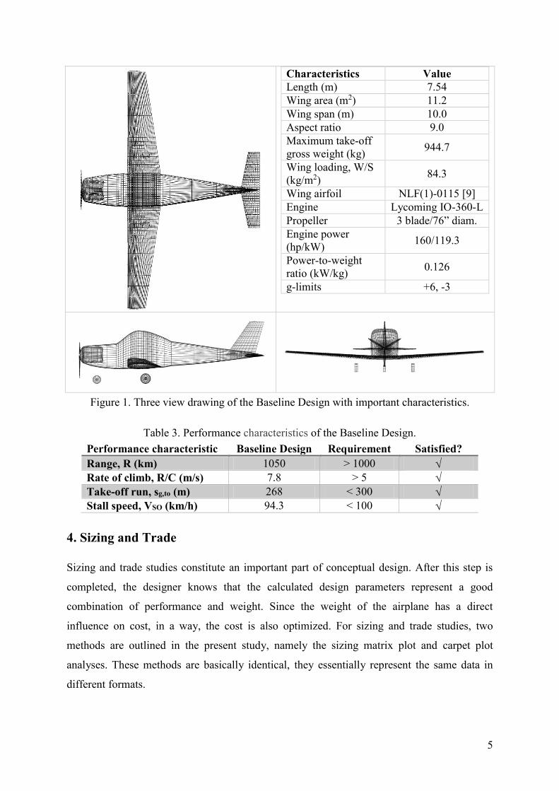
Figure 1 shows the three view drawing of the Baseline Design prepared using OpenVSP [8],
with its important design characteristics. Table 3 compares its performance characteristics
with the requirements given in Table 1. Data in Figure 1 show that the designed airplane falls
into the CS/FAR-23 Classification because of its weight but not the VLA or LSA
Classification. Also, the positive limit load factor selected for the design puts this airplane in
the Aerobatic Category. From Table 3, it can be seen that the airplane satisfies all the
“customer” requirements by a comfortable margin. The questions that remain are: Is this the
best airplane satisfying the requirements? Can a lighter, i.e. greener and less costly airplane to
acquire and operate be designed that can still meet the requirements?
5
Characteristics Value
Length (m) 7.54
Wing area (m2) 11.2
Wing span (m) 10.0
Aspect ratio 9.0
Maximum take-off
gross weight (kg) 944.7
Wing loading, W/S
(kg/m2) 84.3
Wing airfoil NLF(1)-0115 [9]
Engine Lycoming IO-360-L
Propeller 3 blade/76” diam.
Engine power
(hp/kW) 160/119.3
Power-to-weight
ratio (kW/kg) 0.126
g-limits +6, -3
Figure 1. Three view drawing of the Baseline Design with important characteristics.
Table 3. Performance characteristics of the Baseline Design.
Performance characteristic Baseline Design Requirement Satisfied?
Range, R (km) 1050 > 1000
Rate of climb, R/C (m/s) 7.8 > 5
Take-off run, sg,to (m) 268 < 300
Stall speed, VSO (km/h) 94.3 < 100
4. Sizing and Trade
Sizing and trade studies constitute an important part of conceptual design. After this step is
completed, the designer knows that the calculated design parameters represent a good
combination of performance and weight. Since the weight of the airplane has a direct
influence on cost, in a way, the cost is also optimized. For sizing and trade studies, two
methods are outlined in the present study, namely the sizing matrix plot and carpet plot
analyses. These methods are basically identical, they essentially represent the same data in
different formats.

6
4.1. Sizing Matrix Plot
The sizing matrix plot quickly allows the designer to find an optimised combination of
selected design parameters. The outline of the method is as follows:
i. The parameters to be varied or optimized are selected. These are chosen among wing
loading (W/S), thrust-to-weight (T/W) or power-to-weight (P/W) ratio, taper ratio (),
aspect ratio (A), etc. However, as the number of parameters increase, the number of
combinations increase by at least 3n, n being the number of parameters chosen, and the
process becomes more cumbersome. The smallest number of parameters to be chosen
is 2, which means that the minimum number of combinations to be worked with is 9.
Usually, wing loading (W/S) and thrust-to-weight (T/W) or power-to-weight (P/W)
ratios are chosen for the sizing and trade studies since these have the greatest effect on
performance and weight. Actually, in this study, S (trapezoidal wing planform area)
and P (power) are chosen as the trade parameters because the weight estimation
method utilized requires these parameters as inputs.
ii. The Baseline Design is perturbed by ±20% for W/S and ±20% for T/W or P/W. One
can increase the number of “perturbed” designs both for W/S and P/W but this will
result in 5n or 7n designs to work with. In this study, the trapezoidal wing reference
area is perturbed by ±20% and power is varied such that more powerful and less
powerful engines belong to the same engine family as the Baseline Design, which may
not always correspond to ±20% variation. While choosing candidate engines, choosing
engines that have similar sizes to the Baseline Design simplifies the analysis
significantly because the nacelle and the fuselage size will be unaffected from the
engine choice. The trapezoidal wing planform areas and the engines that are studied
are as follows (those of the Baseline Design are underlined):
Wing planform areas: 9.0 m2, 11.2 m2, 13.4 m2.
Engines: Lycoming O-235-F (125 hp), Lycoming IO-360-L (160 hp),
Lycoming IO-360-F (180 hp).
While perturbing the wing planform area, the horizontal and vertical tail sizes (SHT and
SVT) are varied proportionately in order to keep the tail volume ratios (VHT and VVT)
the same as the Baseline Design. This also relieves the designer from the burden of
varying the fuselage length in order keep the tail volume ratio constant.

7
Fuselage size is kept constant for all perturbed designs since the cockpit size and tail
moment will remain constant, independent of the wing size and the powerplant.
Fuel volume is initially kept constant for the sake of simplifying the analysis. If the
available fuel is enough to satisfy the mission requirements (especially the range), the
designer may keep the original fuel volume. If the range requirement is not satisfied,
one needs to increase the fuel volume, which will have an effect on the total weight.
iii. The preliminary sizing matrix is constructed. Table 4 shows the preliminary sizing
matrix constructed for the current design.
Table 4. Preliminary sizing matrix.
S=13.4 m2 S=11.2 m2 S=9.0 m2
P=180 hp Config.1 Config. 2 Config. 3
P=160 hp Config. 4 Config. 5 Config. 6
P=125 hp Config. 7 Config. 8 Config. 9
iv. The performance requirements that will be used for optimization are selected. For a
sound analysis, at least three requirements shall be selected. The chosen requirements
shall be balanced between the ones where wing loading (W/S) has a dominant effect
like the stall speed (VSO) and the landing distance (sg,l), and those where power-to-
weight ratio (P/W) has a dominant effect like the rate of climb (R/C), maximum speed
(Vmax), and take-off distance (sg,to). In this study, the performance requirements chosen
are the range (R), rate of climb (R/C), take-off run (sg,to), and the stall speed (VSO),
which are the “customer” requirements.
v. The empty (Wempty) and take-off gross weights (Wo) of each configuration is
calculated. The empty weights are calculated using the Statistical Weights Method
explained in [5]. This method consists of 14 empirical relations for estimating the
weights of the wing, horizontal tail, vertical tail, fuselage, main landing gear, nose
landing gear, installed engine, fuel system, flight controls, hydraulics, electrical
system, avionics, air conditioning/anti-icing system and furnishings as a function of
design gross weight, ultimate load factor, sizes and the geometric shapes of the major
components, cruise speed of the airplane, dry engine weight, etc. It is highly
recommended to use this method for sizing and trade, although it is a bit more
cumbersome than other less comprehensive weight estimation methods since it results
in a more detailed and accurate weight breakdown.
8
vi. The Aerodynamics module is updated for each configuration. The Aerodynamics
module is a spreadsheet involving calculations of the maximum lift coefficient (CLmax),
parasite drag coefficient (CDO), induced drag factor (K), and the drag polar as a
function of speed and altitude. In these calculations, the effect of high lift devices and
the landing gear are taken into account.
vii. The uninstalled thrust or power data obtained from the engine manufacturer or by
using a scaling approach is analysed in order to obtain the installed thrust values. Here,
the losses due to altitude, power extraction, blockage, compressibility, scrubbing drag,
cooling and miscellaneous drag are calculated and the installed thrust is calculated as a
function of speed and altitude. Here, the methods outlined in [5] are used.
viii. Performance calculations are performed for the requirements selected in step iv.
Stall speed (VSO):
Here, the lift equation is employed with the wing planform size (S) selected for the
configuration in step i, and the maximum lift coefficient (CLmax) calculated in step vi.
Here, the airplane is in landing configuration, where the flaps are fully extended.
SCV2
1LW maxL
2 . (1)
Rate of climb (R/C=dh/dt):
For the calculation of the rate of climb, the specific excess power equation is used,
which can also be used in order to calculate other performance characteristics like the
maximum speed, acceleration, service ceiling and the maximum sustained load factor
that can be achieved at a given altitude and speed [5].
dt
dV
g
V
dt
dh
S
W
q
Kn
S/W
Cq
W
TVP 2DO
s
. (2)
For rate of climb calculations, the load factor n=1 and take-off conditions are used. For
take-off, flaps are partially extended and their effects on the parasite drag coefficient
and induced drag are accounted for.
Take-off run (sg,to):
Take-off distance is calculated using the expression given in equation (3) [5]:
T
2TOAT
Ato,g
K
VKKln
gK2
1s , (3)

9
,W/TKT (4)
2LDOLA KCCC)S/W(2
K
. (5)
In the above equations, μ=0.03 is the coefficient of rolling friction between the runway
and tyres. The parasite drag coefficient, CDO includes the additional drag of the
partially extended flaps and the induced drag factor, K is corrected for the ground
effect. During take-off, the airplane is fairly horizontal so CL≈0.1 is assumed.
Range (R):
Range is calculated from the Bréguet Range Equation [7]:
f
i
power
p
W
Wln
D
L
CR . (6)
In this equation, ηp is the propeller efficiency, calculated as a function of the advance
ratio, J=V∞/nD, n: propeller revolutions per second and D: propeller diameter. The
propeller efficiency is corrected for blockage, compressibility and scrubbing drag
effects. The specific fuel consumption is denoted by Cpower and is dependent on the
engine chosen. For the candidate engines in this study, the specific fuel consumptions
are obtained for the cruise condition from manufacturer’s data and have slightly
different values for the three different engines:
Lycoming O-235-F, Cpower=0.4638 lb/h/hp=0.773*10-6 N/W/s,
Lycoming IO-360-L, Cpower=0.4500 lb/h/hp=0.750*10-6 N/W/s,
Lycoming IO-360-F, Cpower=0.4446 lb/h/hp=0.741x10-6 N/W/s.
L/D is dependent on the weight and the speed of the airplane. In order to maximize
range, a propeller-driven airplane must fly at L/D)max. For the Baseline Design and the
remaining configurations this occurs at a speed around 72 m/s (259 km/h) at the cruise
altitude of 2400m. However, it is seen in the calculations that, cruise flight at a speed
of 280 km/h does not significantly alter the range performance of the airplane.
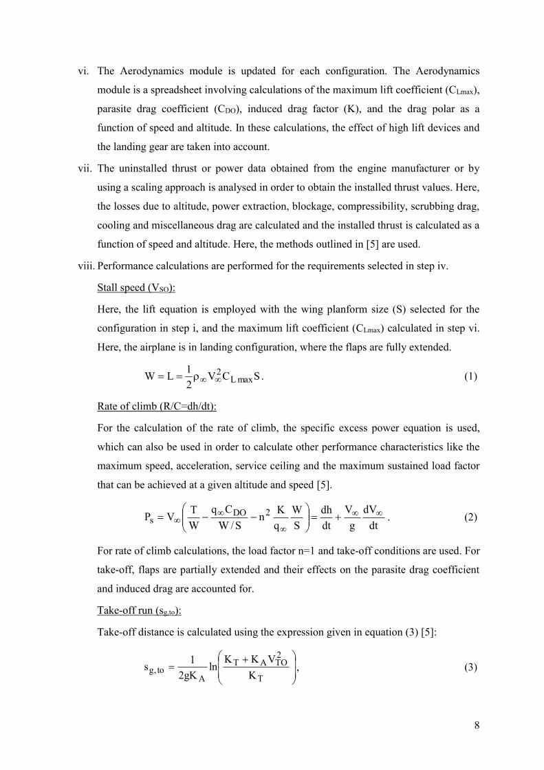
When the performance calculations are performed, the final sizing matrix can be
constructed as can be seen in Table 5. The requirements that are not satisfied are
shown underlined.
From Table 5, we immediately see that the range requirement is satisfied by all 9
configurations. This means that there is no need to vary the fuel weight between
configurations but the range data cannot be used for sizing trade.
10
We also see that there is 100 kg difference between the heaviest (configuration 1) and
the lightest configurations (configuration 9). Configurations 3 and 6 do not satisfy the
stall speed requirement, while the take-off distance requirement is violated by
configurations 7, 8 and 9. Configuration 7, which has the large wing but the small
engine violates the rate of climb requirement also. Configurations 1, 2, 4 and 5 satisfy
all the requirements.
Table 5. Final sizing matrix.
S=13.4 m2 S=11.2 m2 S=9.0 m2
P=180 hp
1
Wo=994.2 kg
VSO=88.5 km/h
R/C=7.9 m/s
sg,to=228 m
R=1006 km
2
Wo=965.4 kg
VSO=95.5 km/h
R/C=8.3 m/s
sg,to=259 m
R=1034 km
3
Wo=937.2 kg
VSO=102 km/h
R/C=9.3 m/s
sg,to=269 m
R=1080 km
P=160 hp
4
Wo=973.2 kg
VSO=87.6 km/h
R/C=7.4 m/s
sg,to=235 m
R=1028 km
5
Wo=944.7 kg
VSO=94.3 km/h
R/C=7.8 m/s
sg,to=268 m
R=1050 km
6
Wo=916.7 kg
VSO=101 km/h
R/C=8.2 m/s
sg,to=292 m
R=1088 km
P=125 hp
7
Wo=950.8 kg
VSO=86.6 km/h
R/C=4.9 m/s
sg,to=319 m
R=1041 km
8
Wo=922.6 kg
VSO=93.4 km/h
R/C=5.2 m/s
sg,to=365 m
R=1061 km
9
Wo=894.9 kg
VSO=99.8 km/h
R/C=5.6 m/s
sg,to=398 m
R=1100 km
ix. The next step is to crossplot the data in Table 5 as illustrated in Figure 2. First, for
each power value, the take-off gross weights are plotted as shown in the first column
of Figure 2. In the plots, hollow circles denote data from Table 5. From the take-off
gross weight graphs of Figure 2, wing areas corresponding to regularly-spaced gross
weights are determined, shown with full circles in the plots. Then the data is
transferred to a wing area (S)-engine power (P) graph as shown in Figure 3. This graph
is already useful as it is because it yields the take-off gross weight for any combination
of wing planform area (S) and engine power (P).

11
Take-off weight, Wo Stall speed, VSO Rate of climb, R/C Take-off distance, sg,to
P=180 hp
P=180 hp
S=13.4 m2
S=13.4 m2
P=160 hp
P=160 hp
S=11.2 m2
S=11.2 m2
P=125 hp
P=125 hp
S=9 m2
S=9 m2
Figure 2. Sizing matrix crossplots.

12
Figure 3. Preliminary sizing matrix plot.
Then, stall speeds, climb rate and the take-off runs are crossplotted in the most convenient
manner as shown in the second, third and fourth columns of Figure 2. In Figure 2, the hollow
circles represent the actual data from Table 5, while full circles correspond to the wing area
(S)-power (P) combinations that exactly meet a given requirement. The combinations that
exactly meet the requirements are transferred to the sizing matrix plot of Figure 3 and joined
by smooth curves, resulting in Figure 4. Again, the hollow circles represent the actual data
from Table 5. These curves constitute the constraint lines and the small arrows indicate the
direction of the feasible region. The Baseline Design is also included in the figure, shown
with a large circle having a dashed outline.
The Optimum Design is the one satisfying all the requirements, having the lowest take-off
gross weight. The Optimum Design will therefore will be at the intersection of two constraint
curves. Hence, the Optimum Design lies at the intersection of the stall and take-off distance
constraint curves, shown with a big black circle at the lower left of the Baseline Design.
4.2. Carpet Plot
As mentioned previously, the carpet plot is an alternative format for presenting the data in
Figure 2. The take-off gross weight plots in the first column of Figure 2 are superimposed as
illustrated in Figure 5. When the data points corresponding to the same wing areas are
connected with straight lines, the resulting shape looks vaguely like a carpet! In the same
13
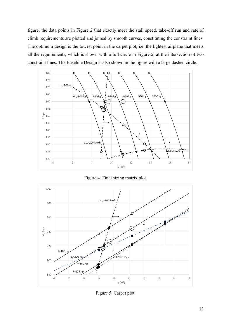
figure, the data points in Figure 2 that exactly meet the stall speed, take-off run and rate of
climb requirements are plotted and joined by smooth curves, constituting the constraint lines.
The optimum design is the lowest point in the carpet plot, i.e. the lightest airplane that meets
all the requirements, which is shown with a full circle in Figure 5, at the intersection of two
constraint lines. The Baseline Design is also shown in the figure with a large dashed circle.
Figure 4. Final sizing matrix plot.
Figure 5. Carpet plot.
14
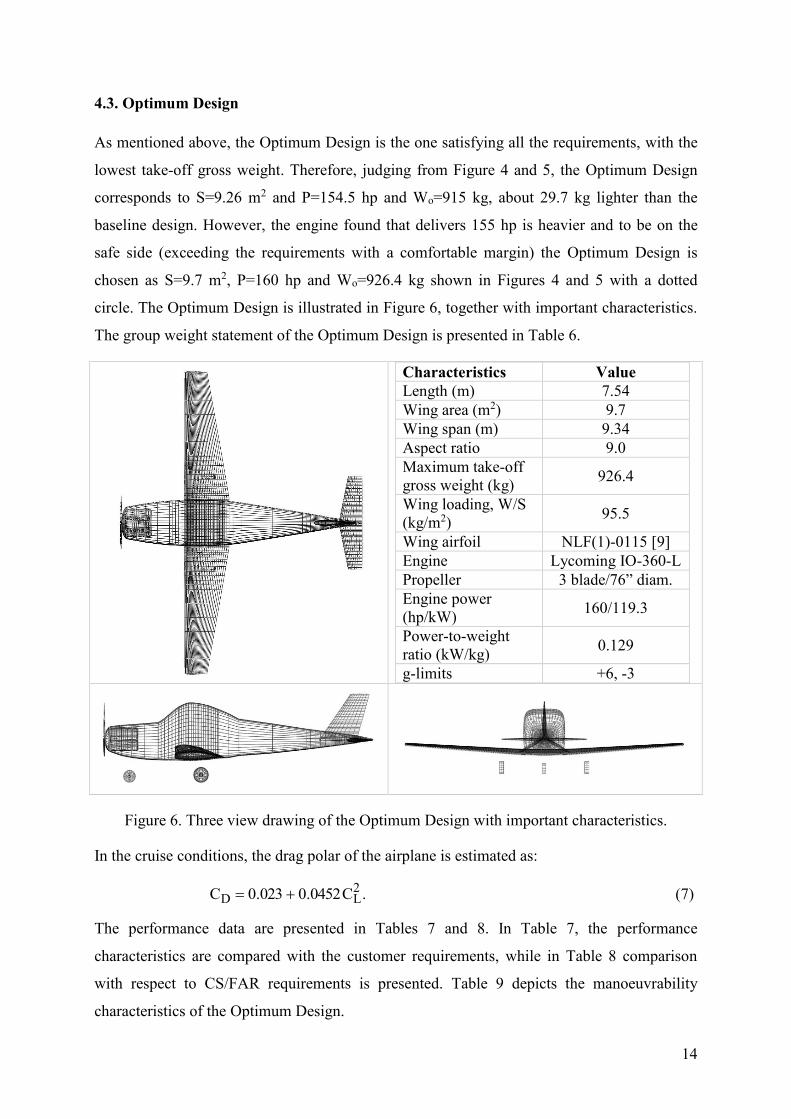
4.3. Optimum Design
As mentioned above, the Optimum Design is the one satisfying all the requirements, with the
lowest take-off gross weight. Therefore, judging from Figure 4 and 5, the Optimum Design
corresponds to S=9.26 m2 and P=154.5 hp and Wo=915 kg, about 29.7 kg lighter than the
baseline design. However, the engine found that delivers 155 hp is heavier and to be on the
safe side (exceeding the requirements with a comfortable margin) the Optimum Design is
chosen as S=9.7 m2, P=160 hp and Wo=926.4 kg shown in Figures 4 and 5 with a dotted
circle. The Optimum Design is illustrated in Figure 6, together with important characteristics.
The group weight statement of the Optimum Design is presented in Table 6.
Characteristics Value
Length (m) 7.54
Wing area (m2) 9.7
Wing span (m) 9.34
Aspect ratio 9.0
Maximum take-off
gross weight (kg) 926.4
Wing loading, W/S
(kg/m2) 95.5
Wing airfoil NLF(1)-0115 [9]
Engine Lycoming IO-360-L
Propeller 3 blade/76” diam.
Engine power
(hp/kW) 160/119.3
Power-to-weight
ratio (kW/kg) 0.129
g-limits +6, -3
Figure 6. Three view drawing of the Optimum Design with important characteristics.
In the cruise conditions, the drag polar of the airplane is estimated as:
.C0452.0023.0C 2LD (7)
The performance data are presented in Tables 7 and 8. In Table 7, the performance
characteristics are compared with the customer requirements, while in Table 8 comparison
with respect to CS/FAR requirements is presented. Table 9 depicts the manoeuvrability
characteristics of the Optimum Design.

15
Table 6. Group statement format of the Optimum Design.
Group Weight (kg)
Structures
Wing
Horizontal tail
Vertical tail
Fuselage
Main landing gear
Nose landing gear
101.1
7.4
4.7
111.3
57.5
18.7
Propulsion
Engine
Fuel system/tanks
176.4
17.4
Equipment
Flight controls
Hydraulics
Avionics
Electrical
Air conditioning & anti-ice
Furnishings
19.4
2.0
30.0
61.0
18.7
24.3
Total empty weight 649.9
Useful load
Crew
Fuel
Payload
160
96.5
20
Take-off gross weight 926.4
Table 7. Performance characteristics of the Optimum Design compared
with customer requirements.
Performance characteristic Optimum Design Requirement Satisfied?
Range, R (km) 1069 > 1000
Rate of climb, R/C (m/s) 6.6 > 5
Take-off run, sg (m) 278.5 < 300
Stall speed, VSO (km/h) 98.0 < 100
Table 8. Performance characteristics of the Optimum Design compared
with CS/FAR requirements.
Performance characteristic Optimum Design Requirement Satisfied?
Stall speed, VSO (km/h) 98.0 < 113 (CS/FAR)
Climb gradient @ VCL, γ 13 % > 8.3% (CS/FAR)
Climb gradient @ VA, γ 9.2% > 3.3% (CS/FAR)
16
Table 9. Manoeuvrability characteristics of the Optimum Design.
Parameter Value
Instantaneous turn rate
Instantaneous turn radius
43.6°/s @ Vcorner = 271 km/h, n=6
98 m @ Vcorner = 271 km/h, n=6
Sustained turn rate
Sustained turn radius
25°/s @ V=245 km/h, n=3.2
155.5 m @ V = 245 km/h, n=3.2
In Table 9, the most forward and backward positions of the centre of gravity with respect to
the mean aerodynamic chord are given together with the corresponding static margin values.
The neutral point is calculated using the method outlined by Etkin and Reid [10]. As can be
seen, the airplane is stiff in longitudinal flight, which can be easily remedied with relocating
certain systems in the airplane during preliminary and detail design phases or moving the
wing a few inches forward.
Table 10. CG positions and longitudinal stability of the Optimum Design.
CG position Chordwise CG position Static margin
Most forward 0.38 16.0 %
Most backward 0.42 12.5 %
Finally, in Table 11, the characteristics of the Optimum Design are compared with those of
competitor aircraft. Seven competitors are chosen, which are: Grob 115E, Grob 120A,
Slingsby T-67, Aermacchi Sf.260D, Cirrus SR.20, Cirrus SR.22, and Diamond DA.20. As can
be seen, the Optimum Design compares well with the competitors. Although it has the
smallest engine except the Diamond DA.20 (which is a VLA Class airplane), it promises
superior performance than the competitors for most of the performance characteristics. It is
also the lightest airplane except for Diamond DA.20. The superior performance is possible
due to laminar flow airfoil, use of smooth moulded composites for the entire airplane that
offers a potential for significant amount of laminar flow (~25% over the fuselage, ~50% over
the wing and tails) and finally optimized weight and performance as explained above. Had a
lighter aeroengine existed delivering 155 hp, it would have been possible to reduce the weight
of the airplane further.
The unit civil purchase price of this airplane is estimated to be $382 000 (€274 000) in 2014
prices estimated using the DAPCA IV Cost Model assuming that 250 airplanes will be
manufactured in 5 years after commencement of production [5].

17
Characteristic Optimum
Design
Grob
G115E
Grob
G120A
Slingsby
T-67
Aermacchi
Sf.260D
Cirrus
SR.20
Cirrus
SR.22
Diamond
DA.20
Performance
Maximum speed (km/h) 360 250 319 281 441 287 339 277
Range (km) 1069 1130 1537 753 2050 1454 1943 1013
Rate of climb (m/s) 6.6 5.3 6.5 7 9.1 4.2 6.5 5.1
Take-off run (m) 278.5 461 707 274 451 295 390
Stall speed (km/h) 98 96 102 100 109 104 111 78
Geometric
Length (m) 7.54 7.54 8.60 7.55 7.00 7.92 7.92 7.16
Wing area (m2) 9.7 12.2 13.3 12.6 10.1 13.7 13.7 11.6
Wing span (m) 9.34 10.00 10.19 10.69 8.22 11.68 11.68 10.87
Aspect ratio 9.0 8.2 7.8 9.1 6.7 10.0 10.0 10.2
Weights
Maximum take-off weight (kg) 926 990 1490 1157 1300 1386 1633 800
Wing loading (kg/m2) 95.5 81.1 112.1 91.8 128.7 101.1 119.1 68.9
Empty weight (kg) 650 685 960 794 675 965 1009 529
Empty weight fraction 0.70 0.69 0.64 0.69 0.52 0.70 0.62 0.66
Power
Engine power (kW) 119 139 190 194 195 149 230 93
Power to weight ratio 0.129 0.140 0.127 0.168 0.150 0.108 0.141 0.116
Table 11. Comparison of the Optimum Design with competitor aircraft (data for competitor aircraft obtained from Internet sources).
18
5. Conclusions
Sizing trade and optimization of a light sport aircraft is outlined. The trade study is performed
for obtaining the optimum wing area-engine power combination. Two methods are described,
namely the sizing matrix plot and carpet plot approaches, both methods having visual
emphasis, which is their main strength. These methods are applicable using widely used
general purpose computational and graphical tools, without the need for costly, dedicated
software. These aspects render the methods suitable for student projects, academic purposes
and also for design of real airplanes in the conceptual design phase. The methods can be
developed further to include a higher number of parameters but then their simplicity and
visual aspects will quickly fade away and programming the methods as a software will
become necessary. The methods are applicable to conventional configurations and should be
used with care when the designed airplane configuration is unconventional like UAVs, tailless
aircraft or aircraft powered by unconventional powerplants like electrical.
While dwelling in the fascinating world of aircraft design, technical knowledge, experience,
and creativity are all vital. On the other hand, it is also beyond doubt that “the airplane” is
aesthetically the most pleasant invention of mankind. We, aircraft designers are privileged to
be following the footsteps of great designers like Marcel Dassault, quote:
„For an aircraft to fly well, it must be beautiful“

19
References
1. European Aviation Safety Agency, Certification Specifications for Normal, Utility,
Aerobatic, and Commuter Category Aeroplanes, CS-23, Amendment 3, 2012.
2. European Aviation Safety Agency, Certification Specifications for Very Light Aeroplanes,
CS-VLA, Amendment 1, 2009.
3. European Aviation Safety Agency, Certification Specifications and Acceptable Means of
Compliance for Light Sport Aeroplanes, CS-LSA, Amendment 1, 2013.
4. Federal Aviation Administration, Airworthiness Standards: Normal, Utility, Acrobatic and
Commuter Category Airplanes, Amendment 55, 2002.
5. Raymer, D. P., Aircraft Design: A Conceptual Approach, 5th Ed., AIAA Education Series,
2012.
6. Roskam, J., Airplane Design, DARCorporation, 1997.
7. Anderson, J. D., Aircraft performance and Design, Mc Graw-Hill, 1999.
8. OpenVSP Core Team, OpenVSP 2.3.0, 2013.
9. Selig, M. S., Maughmer, M. D. and Somers, D. M., Natural-laminar-flow airfoil for general
aviation applications, J. Aircraft 32(4), 1995.
10. Etkin, B. and Reid, L. D., Dynamics of Flight: Stability and Control, John Wiley & Sons,
Inc., 1996.


![UNITED STATES ENVIRONMENTAL PROTECTION … · CARPET- [CLEANER] [CLEANING] - ... Frieze (carpet) Saxony (carpet) Plush (carpet) ... For best results removing tough stains use ...](https://static.fdocuments.in/doc/165x107/5ad777487f8b9a9d5c8c1b4c/united-states-environmental-protection-cleaner-cleaning-frieze-carpet.jpg)