Size Matters - Frankfurt School of Finance & Management
60
econstor Make Your Publications Visible. A Service of zbw Leibniz-Informationszentrum Wirtschaft Leibniz Information Centre for Economics Scholz, Peter Working Paper Size matters! How position sizing determines risk and return of technical timing strategies CPQF Working Paper Series, No. 31 Provided in Cooperation with: Frankfurt School of Finance and Management Suggested Citation: Scholz, Peter (2012) : Size matters! How position sizing determines risk and return of technical timing strategies, CPQF Working Paper Series, No. 31 This Version is available at: http://hdl.handle.net/10419/55526 Standard-Nutzungsbedingungen: Die Dokumente auf EconStor dürfen zu eigenen wissenschaftlichen Zwecken und zum Privatgebrauch gespeichert und kopiert werden. Sie dürfen die Dokumente nicht für öffentliche oder kommerzielle Zwecke vervielfältigen, öffentlich ausstellen, öffentlich zugänglich machen, vertreiben oder anderweitig nutzen. Sofern die Verfasser die Dokumente unter Open-Content-Lizenzen (insbesondere CC-Lizenzen) zur Verfügung gestellt haben sollten, gelten abweichend von diesen Nutzungsbedingungen die in der dort genannten Lizenz gewährten Nutzungsrechte. Terms of use: Documents in EconStor may be saved and copied for your personal and scholarly purposes. You are not to copy documents for public or commercial purposes, to exhibit the documents publicly, to make them publicly available on the internet, or to distribute or otherwise use the documents in public. If the documents have been made available under an Open Content Licence (especially Creative Commons Licences), you may exercise further usage rights as specified in the indicated licence. www.econstor.eu
Transcript of Size Matters - Frankfurt School of Finance & Management

econstorMake Your Publications Visible.
A Service of
zbwLeibniz-InformationszentrumWirtschaftLeibniz Information Centrefor Economics
Scholz, Peter
Working Paper
Size matters! How position sizing determines riskand return of technical timing strategies
CPQF Working Paper Series, No. 31
Provided in Cooperation with:Frankfurt School of Finance and Management
Suggested Citation: Scholz, Peter (2012) : Size matters! How position sizing determines riskand return of technical timing strategies, CPQF Working Paper Series, No. 31
This Version is available at:http://hdl.handle.net/10419/55526
Standard-Nutzungsbedingungen:
Die Dokumente auf EconStor dürfen zu eigenen wissenschaftlichenZwecken und zum Privatgebrauch gespeichert und kopiert werden.
Sie dürfen die Dokumente nicht für öffentliche oder kommerzielleZwecke vervielfältigen, öffentlich ausstellen, öffentlich zugänglichmachen, vertreiben oder anderweitig nutzen.
Sofern die Verfasser die Dokumente unter Open-Content-Lizenzen(insbesondere CC-Lizenzen) zur Verfügung gestellt haben sollten,gelten abweichend von diesen Nutzungsbedingungen die in der dortgenannten Lizenz gewährten Nutzungsrechte.
Terms of use:
Documents in EconStor may be saved and copied for yourpersonal and scholarly purposes.
You are not to copy documents for public or commercialpurposes, to exhibit the documents publicly, to make thempublicly available on the internet, or to distribute or otherwiseuse the documents in public.
If the documents have been made available under an OpenContent Licence (especially Creative Commons Licences), youmay exercise further usage rights as specified in the indicatedlicence.
www.econstor.eu

CCeennttrree ffoorr PPrraaccttiiccaall QQuuaannttiittaattiivvee FFiinnaannccee
CPQF Working Paper Series
CPQF Working Paper Series
No. 31
Size Matters!
How Position Sizing Determines Risk and Return of
Technical Timing Strategies
Peter Scholz
Authors: Peter Scholz Associate Research Fellow CPQF Frankfurt School of Finance & Management
Frankfurt/Main [email protected]
January 2012
Publisher: Frankfurt School of Finance & Management Phone: +49 (0) 69 154 008-0 � Fax: +49 (0) 69 154 008-728 Sonnemannstr. 9-11 � D-60314 Frankfurt/M. � Germany

Size Matters!
How Position Sizing Determines Risk and Return of
Technical Timing Strategies
Peter Scholz
Frankfurt School of Finance & Management
Centre for Practical Quantitative Finance
Working Paper, Version: January 15th, 2012
Abstract
The application of a technical trading rule, which just provides long and short signals,
requires the investor to decide upon the exposure to stake in each trade. Although this
position sizing (or money management) crucially affects the risk and return characteristics,
recent academic literature has largely ignored this effect, leaving reported results incompa-
rable. This work systematically analyzes the impact of position sizing on timing strategies
and clarifies the relation to the Kelly criterion, which proposes to bet relative fractions from
the remaining gambling budget. Both erratic as well as different relative positions, i.e. fixed
proportions of the remaining portfolio value, are compared for simple moving average trad-
ing rules. The simulation of parametrized return series allows systematically varying those
asset price properties, which are most influential on timing results: drift, volatility, and
autocorrelation.
The study reveals that the introduction of relative position sizing has a severe impact on
trading results compared to erratic positions. In contrast to a standard Kelly framework,
however, an optimal position size does not exist. Interestingly, smaller trading fractions
deliver the highest risk-adjusted returns in most scenarios.
Keywords: Kelly Criterion, Money Management, Parameterized Simulation, Position Siz-
ing, Technical Analysis, Technical Trading, Timing Strategy.
JEL Classification: G11
I

II Frankfurt School of Finance & Management — CPQF Working Paper No. 31
Contents
I Introduction 1
II Literature Review 2
IIIMethodology 4
III.1 Parametric Simulation . . . . . . . . . . . . . . . . . . . . . . . . . . . . . . . 4
III.2 The Simple Moving Average Trading Rule . . . . . . . . . . . . . . . . . . . . 5
III.3 The Money Management Component . . . . . . . . . . . . . . . . . . . . . . . 6
III.4 Evaluation Criteria for Trading Systems . . . . . . . . . . . . . . . . . . . . . 7
IV Simulation Results 7
IV.1 Optimality of Fractions . . . . . . . . . . . . . . . . . . . . . . . . . . . . . . . 8
IV.2 Position Sizing Effects for Different Trend Levels . . . . . . . . . . . . . . . . 10
IV.3 Position Sizing Effects for Different Volatility Levels . . . . . . . . . . . . . . . 14
IV.4 Position Sizing Effects for Different Autocorrelation Levels . . . . . . . . . . . 17
V Conclusions 20
List of Figures
1 Terminal wealth relative dependent on fraction . . . . . . . . . . . . . . . . . . . 9
2 Terminal wealth relative dependent on fraction for single paths . . . . . . . . . . 10
3 Return figures dependent on drift . . . . . . . . . . . . . . . . . . . . . . . . . . . 12
4 Risk figures dependent on drift . . . . . . . . . . . . . . . . . . . . . . . . . . . . 13
5 Return figures dependent on volatility . . . . . . . . . . . . . . . . . . . . . . . . 15
6 Risk figures dependent on volatility . . . . . . . . . . . . . . . . . . . . . . . . . . 16
7 Return figures dependent on autocorrelation . . . . . . . . . . . . . . . . . . . . . 19
8 Risk figures dependent on autocorrelation . . . . . . . . . . . . . . . . . . . . . . 20
List of Tables
1 Kelly position sizes. . . . . . . . . . . . . . . . . . . . . . . . . . . . . . . . . . . 8
2 Overview of the 35 selected leading equity indices. . . . . . . . . . . . . . . . . . 25
3 Evaluation criteria . . . . . . . . . . . . . . . . . . . . . . . . . . . . . . . . . . . 26
4 f-25% trade results of different drift levels. . . . . . . . . . . . . . . . . . . . . . . 29
5 f-50% trade results of different drift levels. . . . . . . . . . . . . . . . . . . . . . . 30

Frankfurt School of Finance & Management — CPQF Working Paper No. 31 III
6 f-75% trade results of different drift levels. . . . . . . . . . . . . . . . . . . . . . . 31
7 f-100% trade results of different drift levels. . . . . . . . . . . . . . . . . . . . . . 32
8 f-125% trade results of different drift levels. . . . . . . . . . . . . . . . . . . . . . 33
9 Unsized trade results of different drift levels. . . . . . . . . . . . . . . . . . . . . . 34
10 f-25% trade results of different volatility levels. . . . . . . . . . . . . . . . . . . . 35
11 f-50% trade results of different volatility levels. . . . . . . . . . . . . . . . . . . . 36
12 f-75% trade results of different volatility levels. . . . . . . . . . . . . . . . . . . . 37
13 f-100% trade results of different volatility levels. . . . . . . . . . . . . . . . . . . . 38
14 f-125% trade results of different volatility levels. . . . . . . . . . . . . . . . . . . . 39
15 Unsized trade results of different volatility levels. . . . . . . . . . . . . . . . . . . 40
16 f-25% trade results of different autocorrelation levels. . . . . . . . . . . . . . . . . 41
17 f-50% trade results of different autocorrelation levels. . . . . . . . . . . . . . . . . 42
18 f-75% trade results of different autocorrelation levels. . . . . . . . . . . . . . . . . 43
19 f-100% trade results of different autocorrelation levels. . . . . . . . . . . . . . . . 44
20 f-125% trade results of different autocorrelation levels. . . . . . . . . . . . . . . . 45
21 Unsized trade results of different autocorrelation levels. . . . . . . . . . . . . . . 46

Frankfurt School of Finance & Management — CPQF Working Paper No. 31 1
“[Money Management] — It is not that part of your system that dictates how much you will
lose on a given trade. It is not how to exit a profitable trade. It is not diversification. It is
not risk control. It is not risk avoidance. It is not that part of your system that tells you what
to invest. Instead, [...] it is the part of your trading system that answers the question “How
much?” throughout the course of a trade.”Van K. Tharp (2007)
I Introduction
Technical trading rules usually generate a binary series of buy (1) and sell (0) signals, but do
not provide information how much of the trading budget1 should be invested in every trade.
The part of a trading system, which answers this particular question, is called position sizing or
money management. The choice of the money management policy has a severe impact on trading
results from both a risk and return perspective. The most basic way to follow a trading rule is
unmanaged positions, i.e. always to buy or sell one unit (e.g. one share) of the underlying asset.2
In this case, the position size is erratic because it only depends on the share price and leveraging
may become very large.3 To avoid this, two basic money management techniques can be applied:
absolute positions, i.e. to invest fixed amounts, which is widely preferred by practitioners (Potters
& Bouchaud 2005); or relative positions, i.e. a fixed proportion of the remaining trading capital
as inspired by Kelly (1956).4 In trading systems, however, the original Kelly idea is modified
such that the capital allocation is a dynamic process over time: the investor follows active
trading signals and sizes the trading position relative to the remaining trading budget.
Recent academic literature on technical trading, which primarily focuses on the highly con-
troversial issue of benefits from trading rules, spends surprisingly little attention to describe their
detailed implemented position sizing. As a consequence, different views exist on the applied po-
sition sizes: Fifield, Power & Sinclair (2005), for example, suggest that in previous studies the
investor had an unlimited trading budget, whereas Zhu & Zhou (2009) assume that trading
positions are restricted to 100% of the remaining trading capital; and Anderson & Faff (2004)
suppose that a fixed number of contracts is traded. However, it is more than doubtful that
findings from studies with different implementations are comparable. In practice, experienced
system developers generally are aware of the dilemma of money management: undersized posi-
tions cannot fully exploit the trading rule’s potential, but even promising trading strategies may
1The trading budget is the value of the actively managed portfolio.2To show that asset price characteristics explain timing success, we applied a trading system with unmanaged
positions to analyze the pure influence of the trading rule (Scholz & Walther 2011).3For example, if the remaining trading budget is low and the share price is comparatively high.4In order to achieve an optimal betting strategy, Kelly suggested reinvestment of gainings such that the expected
value of the logarithm of the gambling budget is maximized.

2 Frankfurt School of Finance & Management — CPQF Working Paper No. 31
generate losses if too much exposure is taken.5 Traders are prone to another fallacy, though:
to integrate highly complex money management rules solely on the basis of backtests (Harris
2002). This practice is methodologically weak and never provides a structured insight into the
impact of position sizing on the investment’s risk/return profile.
The present study contributes to the literature by revealing the systematic impact of money
management on a trading systems’ return distribution. The focus thus lies not only on identifying
optimal Kelly strategies or on evaluating the wealth levels achieved. Instead, I compare two basic
money management implementations applied to the prominent simple moving average trading
rule: erratic positions as well as different leveraging levels of relative position sizing. Asset
returns are simulated by parametric stochastic processes, with systematic variations of the most
influential asset price characteristics: the trend (or drift) µ, the volatility of returns σ, and
the first-lag serial autocorrelation parameter ϕ of an AR(1) process. In contrast to standard
backtests, the simulation approach allows to evaluate the return distributions of terminal results
as well as the daily return distributions. Both is done by applying a wide range of popular
statistical-, return-, risk-, and performance figures.
The study documents a severe impact of money management on the overall success or failure
of the trading system and a clear dependence of this impact on the asset price characteristics
of the underlying. In most scenarios, smaller relative trading positions deliver comparatively
high Sharpe ratios. In fact, the introduction and especially the reduction of relative position
sizes offers some kind of protective element: return is sacrificed in order to limit the risks from
timing, especially large drawdowns. However, a universal optimal position size as supposed by
the Kelly criterion does not exist. This finding contradicts Anderson & Faff (2004), who claim
empirical optima based on backtests.
After a brief literature review, Section III explains the methodology in more detail. Section
IV presents the simulation results and summarizes the risk and performance implications from
managed positions. Section V concludes.
II Literature Review
The idea of optimal position sizing goes back to Kelly (1956), who applied information theory on
gambling and proved that the information transfer rate over a channel is equal to the maximum
exponential growth rate of a gambler’s capital. The original Kelly criterion, however, is not
directly applicable in finance since here the outcomes are typically not Bernoulli distributed, in
contrast to many gambling games. It can be shown, though, that maximizing the growth rate
5For example, consecutive losing trades and drawdowns may consume the initial capital before net profits can be
realized.

Frankfurt School of Finance & Management — CPQF Working Paper No. 31 3
is formally achieved by maximizing logarithmic utility. In 1959, Latane put forth the idea of
maximizing logarithmic utility to get an optimal growth rate in an economic context. In many
publications, the U.S. mathematician Edward Thorp adapted the Kelly formula to portfolio
selection (e.g. Thorp 1969, 1971, 1980, 2006, 2010, Rotando & Thorp 1992). Other works on
the subject further elaborated the concepts and worked out implementable solutions (Browne
1999, Hakansson & Ziemba 1995, MacLean, Ziemba & Li 2005, McEnally 1986, Mulvey, Pauling
& Madey 2003, Wilcox 2003a,b, 2005).
In continuous time, the Kelly criterion has two major beneficial long run properties:6 the
asymptotic growth rate is maximized and the time to reach a given wealth level is minimized
(Breiman 1961). Although many scientists consider maximizing the log utility as superior, some
economists vigorously argue against the criterion since it neglects individual investing preferences
in favor of the optimal growth rate. Paul Samuelson (cf. Samuelson 1969, 1971, 1979, Merton
& Samuelson 1974) points out that the application of the Kelly criterion is comparably risky
due to potentially highly levered bets. It could indeed be discouraging for investors to follow
the Kelly strategy since trading success is not guaranteed if the time horizon is finite and
there is a significant potential to interim setback periods (MacLean, Thorp & Ziemba 2010).
MacLean, Ziemba & Blazenko (1992) considered the trade-off between growth by applying the
Kelly criterion and security in terms of drawdowns and found that the high wagers of full Kelly
bets may lead to an immense reduction of wealth. However, fractional Kelly strategies, which
lower the fraction of the original Kelly bet proportionally, may help to overcome these issues by
lowering volatility and reducing the error-proneness in the edge7 calculations (MacLean, Sanegre,
Zhao & Ziemba 2004, MacLean, Zhao & Ziemba 2009). Admittedly, even those who support
Kelly’s idea tend to adopt fractional strategies since one of the fundamental insights of Kelly is
the fact that overbetting is more harmful than underbetting, since it lowers growth but increases
risk (Ziemba 2009).8 MacLean, Thorp, Zhao & Ziemba (2010) confirm this perception since they
find that the full Kelly approach does not stochastically dominate the fractional strategies.
In investment practice, there are many applications for Kelly strategies:9 to allocate capital
between different asset classes (e.g. Heath, Orey, Pestien & Sudderth 1987), to manage the
exposure of the risky asset in a portfolio (e.g. MacLean, Thorp, Zhao & Ziemba 2011), as well
6Cf. MacLean, Thorp & Ziemba (2010) for an extensive discussion about the “good and the bad properties of
the Kelly criterion”.7The term edge denotes the individual advantage over the general public. The determination of the optimal Kelly
bet relies on an estimate of the gambler’s edge: in a portfolio context, edge describes the individually expected
return. In a very simplistic view, the optimal full Kelly bet is the edge divided by the odds (MacLean, Thorp &
Ziemba 2010), i.e. depending on the estimates of the asset’s drift and volatility.8Kelly assumes that if more risk is taken, then the investor increases the probability of extreme outcomes.9Ziemba (2005) lists famous investors which are suspected to use Kelly strategies, including John M. Keynes and
Warren Buffett.

4 Frankfurt School of Finance & Management — CPQF Working Paper No. 31
as to size individual positions within a trading system or stocks in a portfolio (e.g. Anderson &
Faff 2004). In an empirical study, MacLean et al. (2011) analyze the performance of different
Kelly strategies in realistic market scenarios and confirm that in the two asset case (U.S. equity
and T-bills with annual re-balancing) there is a trade-off between terminal wealth and risk:
the more aggressive the Kelly bet, the higher the moments of the terminal wealth distribution.
In contrast to the portfolio selection approach, Anderson & Faff (2004) consider the world of
trading strategies, which implies a dynamic allocation process over time. They size the position
dependent on the remaining trading capital, following the optimal-f money management policy.10
Therefore, Anderson & Faff (2004) do not maximize the utility function of the investor but try
to find the optimal trading size empirically, assuming that such optimum exists. They base
their findings solely on return figures extracted from a backtest of five different future markets,
covering a nine-year period. With this backtest approach they find that money management has
an important impact on trading rule profitability, which supports the perception of real traders.
But, as will be revealed in this study, they were deceived by the incidental sample of their study.
III Methodology
III.1 Parametric Simulation
For the analysis, asset prices are simulated by standard time series models to obtain the entire
return distribution of terminal results. The simulation approach furthermore allows to system-
atically test the influence of different asset price characteristics on the effectiveness of money
management and to exclude certain patterns which may occur in empirical data.
A discretized random walk is used to analyze the impact from the drift (or trend) µ and the
standard deviation (or volatility) σ on trading results. The model is given as
rt = ln
(StSt−1
)=
(µ− σ2
2
)· ∆t + σ ·
√∆t · εt (1)
where St denotes the stock price at time t, ∆t = 1/250 a time interval of one day, and εt a
standard-normal random variable (Glasserman 2003).
Whereas the random walk model creates normally distributed returns, stock market returns
typically exhibit some well-known stylized facts such as fat tails, time varying volatility or
clustering of extreme returns (McNeil, Frey & Embrechts 2005). This is confirmed by the
descriptive statistics of our data sample, where all 35 markets show such non-normality. With
respect to trading results, the most influential amongst the stylized facts are autocorrelated
10As a practitioner, Ralph Vince published a series of books which deal with Kelly-based money management
approaches (cf. Vince 1990, 1992, 1995, 2007). He tries to identify an optimal relative position size f , which is
denoted as optimal-f and which he assumes will maximize the geometric rate of return.

Frankfurt School of Finance & Management — CPQF Working Paper No. 31 5
returns. Statistical tests indicate that short time lags have the strongest impact on future
returns (Cerqueira 2006). Therefore, a first-order autoregressive process AR(1) is applied as
given by rt = ϕ · rt−1 + εt, such that the full model with drift results in
rt =
(µ− σ2
2
)· ∆t + ϕ · rt−1 + σ ·
√∆t · εt. (2)
For every parametric simulation, 10,000 paths were generated, which produced stable re-
sults.11 All paths comprise 2,500 data points, which corresponds to 10 years with 250 trading
days. Additionally, a forerun of prices ensures the availability of an SMA value for the first day.
The initial underlying asset price is always set at 100e.
For the parameterization of the stochastic processes, real world data is used from 35 leading
global equity indices [cf. table (2)]. The database contains daily closing prices from 1 January
2000 to 31 December 2009 taken from Thomson Reuters. The extremes and averages of drift,
volatility, and autocorrelation are put into the parameterized simulations.12
III.2 The Simple Moving Average Trading Rule
A trading rule generally converts information from past prices into a digital series of buy and sell
signals. In contrast to the portfolio selection problem, the trading rule aims to forecast market
movements by indicating rising (1) or falling (0) prices. Accordingly, the exposure is shifted
between the risky benchmark, for example a stock market index, and the risk free alternative,
i.e. cash. The price path, which is finally generated by the trading rule is referred to as equity
curve or active portfolio.
Simple moving averages as a trading rule are a very popular example in the academic litera-
ture. The basic idea is to follow established trends, which are detected by comparing historical
price averages with the current price. SMAs have also been applied in our earlier study as an
example to verify the impact from asset price parameters on trading success. Hence, this trading
rule is also used in this study to ease comparison. The SMA(d)t on day t is the unweighted
average of the previous d asset prices pi (i = t− d− 1, ..., t− 1) excluding the present day t:
SMA(d)t =1
d·
t−1∑i=t−d−1
pi. (3)
If pt ≥ SMA(d)t, then the system indicates a long position, i.e. holding the risky asset. If
pt < SMA(d)t, then the trading budget is entirely invested in cash. In case a buy or sell signal
is triggered, the positions are opened or closed completely.
The practical implementation of an SMA trading rule needs additional specifications (besides
money management): in this study, short positions are not allowed, interest on the risk free cash
11A simulation with 100,000 paths was also run to verify that the results are stable enough.12It should be noted, though, that the empirical levels of the parameters may not be stable over time.

6 Frankfurt School of Finance & Management — CPQF Working Paper No. 31
account as well as dividend payments are not considered, and, in case of levered portfolios, credit
rates do not apply. Lending is possible as long as the net position from debt and the portfolio is
positive. Nevertheless, leverage may cause losses beyond the initial investment and hence imply
the ruin of the investor. If a strategy on a given price path loses the total initial investment then
the strategy stops, the terminal value is set to zero and registered as total loss. All transactions
take place at the very moment when the price of the benchmark is compared to the derived
SMA.13 Sufficient liquidity and an atomistic market are therefore assumed. As SMA intervals,
the 5, 10, 20, 38, 50, 100, and 200 day average are applied.14
III.3 The Money Management Component
In this study, a trading system with unmanaged positions is compared to relative position sizing,
which allows studying the sensitivity of timing results with respect to the money management
policy. If one trading unit of the underlying is bought or sold every time, e.g. one stock,
then the position size is unmanaged, i.e. erratic. This implies uncontrolled leveraging since
the exposure is only dependent on the ratio of stock price and remaining trading budget. The
relative position sizing is inspired by Kelly’s idea of relative wagers and thus reinvestment of
gains. The original Kelly bet follows from maximizing the logarithmic utility function, assuming
normally distributed returns and is given as xK =µr−rfσ2r
with mean µr and variance σ2r of the
risky asset e and the risk-free rate rf (cf. Merton 1992, MacLean et al. 2011). Following a strict
Kelly bet poses various problems, both on the market and on the investor side (shifting input
variables, changing risk tolerance and/or utility preferences of investors, non-normal distribution
of asset returns, Black Swan events etc.). Therefore, it may be appropriate to lower the full
Kelly bet in case of extreme leveraging. If a signal is triggered, feasible portions of 25%, 50%,
75%, 100%, or 125% of the remaining portfolio value are invested in the risky asset. Those
fractions are constant over time and not adjusted to new return or volatility estimates.15
Once a trade is executed, the position remains unadjusted during the whole course of the
trade. After a sell signal is triggered, the position will be closed completely. It is important
to note that the timing signals derive from the technical trading rule only. No additional
instruments to limit the exposure such as stop-loss levels are applied. These assumptions are
meant to ensure, that the pure influence from position sizing is analyzed, not risk management,
transaction costs or interest rate sensitivity.
13In practice, one could assume that the price of the midday auction triggers the SMA and the system buys or
sells at the very next price.14A test with all in-between levels showed a rather smooth development, hence only seven nodes are used.15In general, parameters could be adjusted dynamically.

Frankfurt School of Finance & Management — CPQF Working Paper No. 31 7
III.4 Evaluation Criteria for Trading Systems
The evaluation of an investment’s success has to balance risk and return. While Anderson &
Faff (2004) focus on the return component only, this work also considers the risk element. Due
to the simulation approach, the distribution of terminal results can be analyzed, which delivers
the main findings and describes the investor’s real exposure. Standard backtests, which are
especially popular in practice, are based on the single historical price path and hence deliver a
pathwise distribution only and are thus merely an estimate for the terminal result distribution.
Particularly if the distributions are skewed and “reshaped”, the pathwise distributions may be
a biased estimator. Nevertheless, some key figures are path-dependent; in this case, the mean
over all generated paths is reported (particularly including total profits, total losses, total net
results, and maximum drawdowns.)
For the analysis of the position sizing effect, a broad range of evaluation criteria is applied
(the complete set of criteria is listed in table (3)).16 It turned out that the different measures
mostly delivered comparable information. Even measures which are especially designed for
highly non-normal (reshaped) distributions do not rank investment alternatives differently than
standard measures. While this finding seems to be surprising, it is actually in-line with literature.
I therefore focus on total profits, total losses, total net results, the terminal wealth relative
(TWR),17 maximum drawdowns, the (higher) moments of the return distribution, the value-at-
risk, the Sharpe ratio, and the expected excess return (compared to a buy-and-hold investment)
for the description of timing results.
IV Simulation Results
The results section is structured as follows: first of all, I demonstrate that there is no optimal
position size in trading and that empirical optima are just a statistical artifact [subsection
IV.1]. Subsequently, the impact of introducing a money management policy in a trading system
is revealed. Therefore, in the subsections IV.2 to IV.4, the sensitivity of trading results to
position sizing is analyzed, depending on the properties of the underlying asset price process:
drift, volatility, and autocorrelation. I apply a trading system with unmanaged (or erratic)
positions, which is compared to relative position sizing; trading systems with different levels of
relative positions sizing are also compared. The complete set of results is given in tables (4)
to (21) in the Appendix. Figures (3) to (8) moreover illustrate the results for the maximum
and minimum input variables, found in the empirical dataset (e.g. the maximum and minimum
drift). For reasons of clarity and readability, I abstain from graphically displaying the mean
16Additional figures can be provided upon request in case of particular interest.17The terminal wealth relative is defined as final balance divided by initial account size.

8 Frankfurt School of Finance & Management — CPQF Working Paper No. 31
values of the input variables. Every figure shows six pictures: on the left hand side, the results
for the maximum value of the input variable is shown; and on the right hand side the results
for the minimum value. Each line in a graph shows the results from one specific position sizing
method. The erratic position size as the point of reference is depicted in bold black (marked
with squares). It should be noted that the scaling of the graphs may be very different due to
the absolute performance differences.
Figures (3), (5), and (7) present the profitability figures (total net results, mean returns, and
Sharpe ratios); figures (4), (6), and (8) illustrate the corresponding risk perspective (volatility,
maximum drawdowns, and value-at-risk). All path-dependent values represent the average of
the 10,000 simulated paths.
Model Parameter Max Mean Min
Brownian motion with varying drift µ 22.6% 5.2% -11.6%
σ 26% 26% 26%
Kelly size 334% 77% -118%
Brownian motion with varying volatility µ 5.2% 5.2% 5.2%
σ 39% 26% 16%
Kelly size 34% 77% 203%
AR(1) with varying autocorrelation µ 5.2% 5.2% 5.2%
σ 26% 26% 26%
ϕ 0.201 0.025 -0.103
Kelly size 77% 77% 77%
Table 1: Kelly position sizes. The table displays the Kelly position sizes with respect to
the three different scenarios, in which either the drift, the volatility, or the autocorrelation is
sensitive. The Kelly size corresponds to the relative amount of risky assets compared to the
remaining trading capital. Negative numbers imply short positions.
IV.1 Optimality of Fractions
Considering portfolio selection problems, the Kelly criterion provides optimal position sizes,
at least if returns are normally distributed and the investment horizon is infinite. It is thus
possible to determine optimal position sizes by applying the Kelly criterion. The question is,
whether or not the Kelly formula also allows to find optimal position sizes in trading systems,
in which the capital allocation is triggered by trading signals and thus develops as a dynamic
process over time. To begin with, the Kelly position sizes for the scenarios analyzed in this study

Frankfurt School of Finance & Management — CPQF Working Paper No. 31 9
are determined, which are dependent on trend and volatility of the underlying asset. For the
Brownian motion, the normality assumption is fulfilled and the application of the Kelly formula
is possible in principal. Autocorrelated returns do generally not qualify for Kelly bets, however,
the corresponding level for normal distributed returns is used as a reference. The full Kelly
wagers are given in table (1), assuming a risk-free rate of 0%.
Figure 1: Terminal wealth relative dependent on fraction. The graph displays the
dependency between the TWR and the applied fraction of the trading strategy. Every line
stands for a different trading rule. Interestingly, there is no optimal terminal wealth relative
but a monotone gradient, by contrast to the findings of the classical portfolio application of
Kelly fractions. This finding holds for different drift, volatility, and autocorrelation levels in the
underlying. The example is based on µ=0.052 and σ = 0.26.
To test for optimal position sizes, I follow Anderson & Faff (2004) who use the terminal
wealth relative (TWR)18 as success measure and plot the growth rate against the corresponding
position size. The highest TWR indicates the best fraction to be used as position size. If an
optimal fraction exists then the chart should show an unique peak. Anderson & Faff (2004)
indeed identified distinctive concave curves and thus derived optimal fractions. However, their
findings are solely based on the one realized price path of the respective underlying. In this
study, I carry out the same analysis for each of the 10,000 simulated paths and take the average.
Interestingly, for this average, the optimal fraction vanishes and there is a monotone gradient
(cf. figure (1)). This finding holds also for the level of the Kelly fraction, which I derived from
the underlying processes. Considering the single paths from the simulation, there is indeed a
18The analysis was also carried out with the logarithm of the terminal wealth as in MacLean et al. (2011). As
expected, this delivers similar findings.
10 Frankfurt School of Finance & Management — CPQF Working Paper No. 31
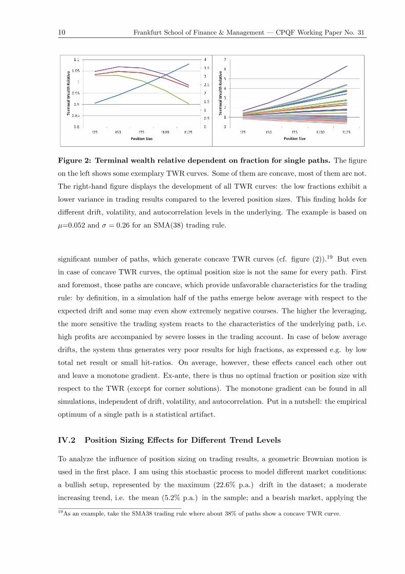
Figure 2: Terminal wealth relative dependent on fraction for single paths. The figure
on the left shows some exemplary TWR curves. Some of them are concave, most of them are not.
The right-hand figure displays the development of all TWR curves: the low fractions exhibit a
lower variance in trading results compared to the levered position sizes. This finding holds for
different drift, volatility, and autocorrelation levels in the underlying. The example is based on
µ=0.052 and σ = 0.26 for an SMA(38) trading rule.
significant number of paths, which generate concave TWR curves (cf. figure (2)).19 But even
in case of concave TWR curves, the optimal position size is not the same for every path. First
and foremost, those paths are concave, which provide unfavorable characteristics for the trading
rule: by definition, in a simulation half of the paths emerge below average with respect to the
expected drift and some may even show extremely negative courses. The higher the leveraging,
the more sensitive the trading system reacts to the characteristics of the underlying path, i.e.
high profits are accompanied by severe losses in the trading account. In case of below average
drifts, the system thus generates very poor results for high fractions, as expressed e.g. by low
total net result or small hit-ratios. On average, however, these effects cancel each other out
and leave a monotone gradient. Ex-ante, there is thus no optimal fraction or position size with
respect to the TWR (except for corner solutions). The monotone gradient can be found in all
simulations, independent of drift, volatility, and autocorrelation. Put in a nutshell: the empirical
optimum of a single path is a statistical artifact.
IV.2 Position Sizing Effects for Different Trend Levels
To analyze the influence of position sizing on trading results, a geometric Brownian motion is
used in the first place. I am using this stochastic process to model different market conditions:
a bullish setup, represented by the maximum (22.6% p.a.) drift in the dataset; a moderate
increasing trend, i.e. the mean (5.2% p.a.) in the sample; and a bearish market, applying the
19As an example, take the SMA38 trading rule where about 38% of paths show a concave TWR curve.

Frankfurt School of Finance & Management — CPQF Working Paper No. 31 11
minimum drift (-11.6% p.a.) from the sample.20 All drift levels are combined with the empirical
mean volatility level of 26% p.a. Tables (4) to (9) contain the detailed results.
Relative versus Erratic Positions In bull markets, the total net result is always positive
and generally highest if no money management component is applied. In bear markets, the
outcome of erratic trading positions is negative but on comparable levels as the 100% fraction.
If we now compare the erratic strategy with the flock of relative ones by considering the relative
position of the black curve (with squares) against the others, we find similar effects for the mean
return. But the erratic position is always inferior to the 100% relative position size, independent
of the market conditions.
With respect to risk-adjusted returns, however, trading systems with relative position sizing
clearly deliver better results than erratic positions. While this clearly holds for bull markets,
this is also the case in bear markets on closer examination. For negative returns, the Sharpe
ratio is misleading, since higher volatilities reward a higher ratio (Scholz & Wilkens 2006). If
the Sharpe ratio is decomposed then it becomes clear that unmanaged positions always raise
the volatility of the equity curve, especially for short term SMAs. The reason for the increase
is the high and uncontrolled leverage, which may occur if the position size is erratic. Since the
short term SMAs trigger more trades, the risk of trading extremely levered positions is higher
than in the less reactive long term SMAs. Furthermore, the introduction of (relative) money
management improves skewness and kurtosis of the trading system’s return distribution [see
table (4) to (9) in Appendix]. The maximum drawdowns, by contrast to volatilities, are on
high but comparable levels in bear markets, if the 100% and 125% fractions are considered as
a reference. In the bullish scenario, the relative position sizing is capable of effectively reducing
the risk from drawdowns. In rising markets, the value-at-risk levels again show the riskiness
of erratic positions, especially if short term SMAs are applied. The introduction of money
management based on relative positions clearly improves the tail risk, except for long SMAs in
bullish environments. In bear markets, only the levered f-125% delivers higher tail risks than
erratic positions. If compared to the underyling asset, erratic positions lead to similar results
as the highly levered (f-125%) portfolio: a small underperformance in terms of expected excess
return in bullish markets; and comparatively poor expected excess returns if medium or negative
drifts are applied.
Different Leverage Levels Relative positions are assumed to correspond to Kelly strategies,
which also recommend constant relative fractions as position sizes. In comparison to the full
20To correct for the volatility drag, the drifts µe measured in the descriptive analysis must be transformed into
µa = µe + 12· σ2 to generate the applied drift levels.

12 Frankfurt School of Finance & Management — CPQF Working Paper No. 31
Figure 3: Return figures dependent on drift. The graphs show the total net results, the
mean returns, and the Sharpe ratio for managed and unmanaged position sizing. On the left,
the results for maximum drift are displayed. On the right, the results for the minimum drift are
shown.
Kelly position size, the applied positions are undersized in bull markets (Kelly ratio of 334%)
and oversized in bear markets (Kelly ratio of -118%). In markets with the average trend of
5.2% p.a., the applied range of f-25% to f-125% lies near the full Kelly size of f-77% (in terms
of portfolio fractions).
Regarding the absolute outcomes in case of positive drifts, the different fractions behave
proportional to the drift component: the higher the leveraging, the higher the profits, the losses
and hence total net results. If negative drifts apply, however, then all systems lose likewise,
with high fractions generating more losses than low fractions. As expected, those findings are
also reflected by the mean returns: in bullish markets (µ = 0.226), the mean return of the
distribution of terminal results falls as the leverage decreases; if medium drifts apply, then the
Frankfurt School of Finance & Management — CPQF Working Paper No. 31 13
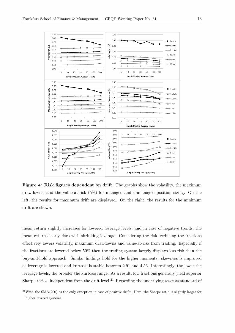
Figure 4: Risk figures dependent on drift. The graphs show the volatility, the maximum
drawdowns, and the value-at-risk (5%) for managed and unmanaged position sizing. On the
left, the results for maximum drift are displayed. On the right, the results for the minimum
drift are shown.
mean return slightly increases for lowered leverage levels; and in case of negative trends, the
mean return clearly rises with shrinking leverage. Considering the risk, reducing the fractions
effectively lowers volatility, maximum drawdowns and value-at-risk from trading. Especially if
the fractions are lowered below 50% then the trading system largely displays less risk than the
buy-and-hold approach. Similar findings hold for the higher moments: skewness is improved
as leverage is lowered and kurtosis is stable between 2.91 and 4.56. Interestingly, the lower the
leverage levels, the broader the kurtosis range. As a result, low fractions generally yield superior
Sharpe ratios, independent from the drift level.21 Regarding the underlying asset as standard of
21With the SMA(200) as the only exception in case of positive drifts. Here, the Sharpe ratio is slightly larger for
higher levered systems.

14 Frankfurt School of Finance & Management — CPQF Working Paper No. 31
comparison, the reduction of leveraging leads to typical protection characteristics: the expected
excess returns suffer in bullish markets but flourish in bearish ones.
Conclusions If positive drift levels apply, then the erratic position sizing seems to be the most
profitable implementation. In case of negative trends, however, the profit and loss figures lie well
within the range given from relative position sizing. The application of relative position sizing
in trading systems effectively lowers the risk from timing compared to erratic positions. The
exact benefit is dependent on the drift level, though. In general, smaller position sizes have a
protection effect, i.e. mean returns are smaller but risk is effectively reduced. Interestingly, the
lowest fraction of 25% has generally better Sharpe ratios than highly levered portfolios (f-125%),
i.e. leveraging does not pay a risk premium. This finding holds in every market scenario.
IV.3 Position Sizing Effects for Different Volatility Levels
For erratic position sizing, we found a negative impact from rising volatility on trading results
(Scholz & Walther 2011). To analyze the sensitivity of trading systems with different position
sizes on volatility, a Brownian motion is again applied (with mean drift level of 5.2% p.a.). I
check for the maximum (39%), the mean (26%), and the minimum (16%) annual volatility levels
given in the empirical dataset.22 The results from volatility influence can be found in tables
(10) to (15) and figures (5) to (6).
Relative versus Erratic Positions If the total net result is considered then the erratic
position sizing is amongst the most profitable implementations, no matter how volatile the
underlying is. In terms of mean returns, the picture however changes: the erratic position sizing
suffers in case of high and medium volatilities of the underlying. This is due to a significant
number of total losses if erratic position sizing is applied. Log-returns weigh the impact of a
total loss stronger than the P&L of a trading account. Only in case of low volatility levels in
the markets, the erratic position sizing generates returns, which are akin to the f-100% and f-
125% implementation. Similar findings hold for risk-adjusted returns: trading systems without
money management clearly underperform in the given volatility setups. A high volatility level
is generally disadvantageous for erratic position sizing under risk aspects: the volatility of the
equity curve is higher, the maximum drawdowns are larger, and the value-at-risk (5%) signals
a high tail-risk. This is confirmed by skewness as well as kurtosis of the equity curve’s return
distribution, which reach extreme levels. Here, introducing relative position sizing really adds
22To cope with the drag effects, the mean drift of 0.052 was adjusted with µa = µe + 12· σ2
a (with σ2a being the
applied volatility level in the simulation) since I intended to measure the volatility effect on the timing result
only, not the mixed influence including effects on the drift component.

Frankfurt School of Finance & Management — CPQF Working Paper No. 31 15
value. In case of comparably low volatility levels of the underlying, however, the introduction
of a relative money management policy has a minor impact; the risk from erratic positions still
approximates the risk from the 125% levered position size and is thus in the upper range.
Figure 5: Return figures dependent on volatility. The graphs show the total net results,
the mean returns, and the Sharpe ratio for managed and unmanaged position sizing. On the
left, the results for maximum volatility are displayed. On the right, the results for the minimum
volatility are shown.
Different Leverage Levels The applied levels of leverage may again be compared to the
corresponding Kelly wagers. A low volatility environment requires high leveraging (203%),
whereas fractions of 34% have to be chosen for high volatilities; for the medium volatility level,
a fraction of 77% corresponds to the Kelly size. Except for the highest fractions, those levels
are covered by the applied position sizes.

16 Frankfurt School of Finance & Management — CPQF Working Paper No. 31
Figure 6: Risk figures dependent on volatility. The graphs show the volatility, the
maximum drawdowns, and the value-at-risk (5%) for managed and unmanaged position sizing.
On the left, the results for maximum volatility are displayed. On the right, the results for the
minimum volatility are shown.
As one would expect, lower fractions decrease the profit potential in the trading account:
the total net result, as well as total profits and losses shrink with the position size, independent
of volatility levels. This finding is also reflected by the mean returns, which slightly decrease in
case of deleveraging.23 Interestingly, if the risk-adjusted returns are examined then the lower
fractions are more appealing: their Sharpe ratios are slightly higher compared to the levered
positions. In turbulent markets, these differences are bigger than in calm markets. Since lower
23High volatility of the underlying asset generally leads to higher trading profits in absolute terms, but not to
higher mean returns. Surprisingly, the strategy’s success with relative position sizing is nearly independent from
the leverage. This effect arises from the log-return effect. Since the erratic approach produces a high number
of paths, which lead to a total loss, it delivers extremely negative return values in the log-return calculation.
Frankfurt School of Finance & Management — CPQF Working Paper No. 31 17
fractions yield less returns, the source must be the risk side. Relative position sizing indeed
effectively reduces the volatility of the underlying. Downsizing of the position size additionally
increases this effect. Moreover, the higher the input volatility, the stronger the reduction effect.
This finding is also confirmed by the maximum drawdowns, which may be disastrous in case of
high volatility in the underlying returns and highly levered positions sizes. A lower fraction can
attenuate the drawdowns to more acceptable levels, especially in highly volatile environments.
The value-at-risk levels also indicate the risk reduction by delevered fractions: tail risks slightly
decrease if the position size is lowered. With respect to the underlying benchmark, the expected
excess returns are rather insensitive to the tested volatility levels.
Conclusions If only the total net result is considered, then the erratic positions work fine. The
moments of the trading system’s return distribution, however, clearly show that relative position
sizing is superior: especially if the underlying exhibits high volatility, the money management
effectively decreases risks. Only in case of low volatile underlyings, the reduction effect is
negligible. Low fractions further reduce the moments but only slightly improve the risk-adjusted
returns.
IV.4 Position Sizing Effects for Different Autocorrelation Levels
In order to analyze the relevance of autocorrelation, an AR(1) process is used to generate
autocorrelated return series. In all simulations, the drift is set at the empirical mean return
level of 5.2% p.a. and the volatility at the empirical mean volatility level of 26% p.a.24 Three
different lag-one autocorrelation levels are examined: the maximum (0.2064), the mean (0.025),
and the minimum (-0.1027) of the empirical estimates from the dataset. An overview of the
results can be found in tables (16) to (21). Figures (7) and (8) display the findings for the
highest and lowest autocorrelation levels.
Relative versus Erratic Positions In highly autocorrelated markets (ϕ = 0.2064), erratic
positions generate positive total net results, which are similar to those of 50% to 75% fractions. In
case of negative autocorrelation, however, the success of erratic positions extremely depends on
the moving average window (low total and mean returns for short windows, higher for long ones).
The SMA(38) seems to be the pivotal point. Especially short term SMA trading rules are prone
to whiplash signals since they respond quickly to the underlying. Erratic positions aggravate this
effect by uncontrolled leveraging; hence they are particularly susceptible to repeated loss trades.
The mean returns generally confirm these findings; due to the log-return calculation, however,
24Once more, the applied drifts have to be corrected with µa = µe · (1−ϕ); and the volatilities σa = σ2e · (1−ϕ2).
18 Frankfurt School of Finance & Management — CPQF Working Paper No. 31
erratic positions generate inferior mean returns.25 If risk-adjusted returns are considered, the
picture slightly changes such that the erratic positions generate inferior Sharpe ratios due to
lower returns and increased volatility. Looking at the risk measures, erratic position sizing
produces extreme risks in the negative autocorrelation scenario: volatility is excessive, maximum
drawdowns may be disastrous, and the value-at-risk indicates a very high tail risk. This is again
due to the susceptibility to whiplash signals. Consequently, in case of positive autocorrelation,
trading systems without position sizing do not cause extended risks. If the trading systems’
returns are compared with those from the underlying asset, the expected excess returns imply
that the erratic positions are inferior to the money-managed trading systems, no matter which
leveraging is applied or which autocorrelation level is used for the simulations.
Different Leverage Levels Although underlyings with autocorrelated returns do generally
not qualify to implement Kelly strategies, the corresponding level for normally distributed re-
turns of 77% is used as a reference. That way, the impact on trading results can be analyzed in
case Kelly sizing is nevertheless applied by investors.
For positive autocorrelation, the total net result is the higher, the higher the leverage. Es-
pecially the short term SMA trading rules benefit, while the long term SMAs are less sensitive
due to a smaller number of trades. Higher leveraging is unfavorable for short term SMAs in this
scenario, however, long term SMAs even benefit from leveraging since they are less sensitive to
whiplash signals. These findings are confirmed by the mean returns of the distribution of ter-
minal results. Independent from the autocorrelation level, a lower leverage improves the Sharpe
ratio of the trading system. Compared to the underlying, however, the f-125% trading system
delivers the highest expected excess returns against the benchmark if positive autocorrelation
applies. The picture changes for negative autocorrelated underlyings and the lower fractions
show the least poor expected excess returns. The implementation of a relative money man-
agement component effectively controls the risk of the active portfolio: excess volatility against
the underlying never occurs, even if highly levered f-125% positions are traded. The skewness
improves in the trading portfolio and the kurtosis rises only moderately (4.64), which implies
that the number of extreme outcomes is only slighly raised. Lower fractions of the position
size moreover reduce the maximum drawdowns and the value-at-risk from timing. The only
exception is the value-at-risk for high serial autocorrelation levels in the underlying: here, the
short term SMA trading rules benefit if they are combined with highly levered trading positions.
Conclusions In terms of profitability, highly levered portfolios are preferable if markets ex-
hibit positive autocorrelation, while unlevered portfolios are better suited if autocorrelation is
25Total net results which imply high losses in the trading account deliver highly negative return figures.

Frankfurt School of Finance & Management — CPQF Working Paper No. 31 19
Figure 7: Return figures dependent on autocorrelation. The graphs show the total net
results, the mean returns, and the Sharpe ratio for managed and unmanaged position sizing.
On the left, the results for maximum autocorrelation are displayed. On the right, the results for
the minimum autocorrelation are shown.
negative (this is consistent with the fact that SMA-timing is highly successful in autocorrelated
markets but suffers from negative autocorrelation). The effect remains, that in positive autocor-
related markets short term SMAs are preferable (and long term SMAs if negative autocorrelation
applies). Risk can be effectively controlled by relative position sizing, especially for lower frac-
tions. Erratic positions are inferior, particularly if markets show negative autocorrelation. The
cautious approach with trading lower fractions thus generates the highest risk-adjusted returns.

20 Frankfurt School of Finance & Management — CPQF Working Paper No. 31
Figure 8: Risk figures dependent on autocorrelation. The graphs show the volatility, the
maximum drawdowns, and the value-at-risk (5%) for managed and unmanaged position sizing.
On the left, the results for maximum autocorrelation are displayed. On the right, the results for
the minimum autocorrelation are shown.
V Conclusions
The study shows that position sizing has a considerable impact on the performance of SMA
timing strategies. Academic papers, which spend only little attention to detailed money man-
agement, miss an important influencing factor and run the risk of misinterpreting or insufficiently
understanding the empirical results. A clear recommendation for optimal position sizes is given
by the well known Kelly ratio, which is applicable in gambling and long-term portfolio allocation.
However, the application of relative positions in trading systems, is different to the “traditional”
Kelly strategies, in which the capital is always invested with a fractional or full Kelly proportion

Frankfurt School of Finance & Management — CPQF Working Paper No. 31 21
in the risky asset. An active trading strategy proposes investments only for specific time periods
according to the signal.
A major finding of the study is that there is no optimal position size in a trading system
which is based on the SMA trading rule. By contrast to portfolio optimization, where generally
a maximum of the terminal wealth relative can be found, the terminal wealth relative of the
trading account is linear and shows no turning point at the Kelly ratio. Findings from other
authors, which suggest that there is an optimal position size, rely on single paths of a backtest.
This is, however, misleading. If the terminal distribution of total net results is considered, then
the concave shape vanishes. Hence, there seems to be no optimal money management approach;
the choice is rather dependent on the underlying asset price characteristics. For instance, if the
underlying shows positive trends, high serial autocorrelation, and/or low volatility, then erratic
or highly levered position management provide fair results. In contrast, if negative drifts, neg-
ative autocorrelation, and/or high volatilities apply, then relative position management is the
better choice. In any case, the introduction of relative money management effectively reduces
the risks in the actively managed portfolio. The exclusive focus on return aspects from money
management hence fails to meet the real strong point of relative position sizing and the major
distinguishing feature to unmanaged positions. If relative position sizing is implemented, how-
ever, then the difference between the diverse fractions is surprisingly small. Interestingly, the
lowest fraction f-25% shows the highest Sharpe ratios amongst the tested portions but not the
highest returns. In terms of risk-adjusted returns, this confirms Kelly’s suggestion that overbet-
ting is more harmful than underbetting. In a nutshell, all-in actually seems not to be the wisest
investment strategy for investors.
Acknowledgments
I am grateful to Leonard C. MacLean from Dalhousie University and Ursula Walther from Frankfurt
School of Finance & Management for helpful discussion and suggestions. The dataset from Thomson
Reuters is very much appreciated. Furthermore, I want to thank the members of the Centre for Practical
Quantitative Finance and the participants of the 19th Triennial Conference of the International Federation
of Operational Research Societies (Melbourne, Australia) for comments and feedback.
References
Anderson, J. A. & Faff, R. W. (2004), ‘Maximizing Futures Returns Using Fixed Fraction Asset
Allocation’, Applied Financial Economics 14, 1067–1073.
Breiman, L. (1961), Optimal Gambling System for Favorable Games, in ‘Proceedings of the 4th
Berkely Symposium on Mathematical Statistics and Probability 1’, pp. 63–78.
Browne, S. (1999), ‘The Risk and Rewards of Minimizing Shortfall Probability’, Journal of
Portfolio Management 25(4), 76–85.

22 Frankfurt School of Finance & Management — CPQF Working Paper No. 31
Cerqueira, A. (2006), Autocorrelation in Daily Stock Prices. Working Paper, 4th PFN Confer-
ence.
Fifield, S. G. M., Power, D. M. & Sinclair, C. D. (2005), ‘An Analysis of Trading Strategies in
Eleven European Stock Markets’, The European Journal of Finance 11(6), 531–584.
Glasserman, P. (2003), Monte Carlo Methods in Financial Engineering, first edn, Springer, New
York.
Hakansson, N. H. & Ziemba, W. (1995), Capital Growth Theory, in ‘Handbooks in OR & MS’,
Elsevier, North Holland, pp. 65–86.
Harris, M. (2002), ‘Facing the Facts of Risk and Money Management’, Active Trader May, 33–
35.
Heath, D., Orey, S., Pestien, V. & Sudderth, W. (1987), ‘Minimizing or Maximizing the Expected
Time to Reach Zero’, SIAM Journal on Control and Optimization 25(1), 195–205.
Kelly, J. L. (1956), ‘A New Interpretation of Information Rate’, The Bell System Technical
Journal 35, 917–926.
Latane, H. A. (1959), ‘Criteria for Choice Among Risky Ventures’, The Journal of Political
Economy 67(2), 144–155.
MacLean, L. C., Sanegre, R., Zhao, Y. & Ziemba, W. T. (2004), ‘Capital Growth with Security’,
Journal of Economic Dynamics and Control 28(5), 937–954.
MacLean, L. C., Thorp, E. O., Zhao, Y. & Ziemba, W. T. (2010), Medium Term Simulations of
the Full Kelly and Fractional Kelly Investment Strategies. Working Paper.
MacLean, L. C., Thorp, E. O., Zhao, Y. & Ziemba, W. T. (2011), ‘How Does the Fortune’s For-
mula Kelly Capital Growth Model Perform?’, The Journal of Portfolio Management 37(4), 96–
111.
MacLean, L. C., Thorp, E. O. & Ziemba, W. T. (2010), Good and Bad Properties of the Kelly
Criterion. Working Paper.
MacLean, L. C., Zhao, Y. & Ziemba, W. (2009), Optimal Capital Growth with Convex Loss
Penalties. Working Paper, Dalhouse University.
MacLean, L. C., Ziemba, W. T. & Blazenko, G. (1992), ‘Growth versus Security in Dynamic
Investment Analysis’, Management Science 38(11), 1562–1585.

Frankfurt School of Finance & Management — CPQF Working Paper No. 31 23
MacLean, L. C., Ziemba, W. T. & Li, Y. (2005), ‘Time to Wealth Goals in Capital Accumulation
and the Optimal Trade-Off Growth versus Security’, Quantitative Finance 5(4), 343–357.
McEnally, R. W. (1986), ‘Latane’s Bequest: The Best of Portfolio Strategies’, Journal of Port-
folio Management 12(2), 21–30.
McNeil, A. J., Frey, R. & Embrechts, P. (2005), Quantitative Risk Management, Princeton Series
in Finance, New Jersey.
Merton, R. C. (1992), Continuous-Time Finance, Blackwell Publishers, Oxford, Melbourne,
Berlin.
Merton, R. C. & Samuelson, P. A. (1974), ‘Fallacy of the Log-Normal Approximation to Optimal
Portfolio Decision-Making Over Many Periods’, Journal of Financial E 1, 67–94.
Mulvey, J. M., Pauling, W. R. & Madey, R. E. (2003), ‘Advantages of Multiperiod Portfolio
Models’, Journal of Portfolio Management 29(2), 35–45.
Potters, M. & Bouchaud, J.-P. (2005), ‘Trend Followers Lose More Often Than They Gain’,
Wilmott Magazine 26, 58–63.
Rotando, L. M. & Thorp, E. O. (1992), ‘The Kelly Criterion and the Stock Market’, The
American Mathematical Monthly 99(10), 922–931.
Samuelson, P. A. (1969), ‘Lifetime Portfolio Selection by Dynamic Stochastic Programming’,
Review of Economics and Statistics 51, 239–246.
Samuelson, P. A. (1971), ‘The “Fallacy” of Maximizing the Geometric Mean in Long Sequences
of Investing or Gambling’, Proceedings of the National Academy of Sciences of the United
States of America 68(10), 2493–2496.
Samuelson, P. A. (1979), ‘Why We Should not Make Mean Log of Wealth Big Though Years to
Act are Long’, Journal of Banking & Finance 3(4), 305–307.
Scholz, H. & Wilkens, M. (2006), ‘Die Marktphasenabhangigkeit der Sharpe Ratio —
Eine empirische Untersuchung fur deutsche Aktienfonds’, Zeitschrift fur Betriebswirtschaft
76(12), 1275–1302.
Scholz, P. & Walther, U. (2011), The Trend is not Your Friend! Why Empirical Timing Success
is Determined by the Underlying’s Price Characteristics and Market Efficiency is Irrelevant.
CPQF Working Paper No. 29, Frankfurt School of Finance & Management.

24 Frankfurt School of Finance & Management — CPQF Working Paper No. 31
Tharp, V. K. (2007), Trade Your Way to Financial Freedom, second edn, McGraw-Hill, New
York.
Thorp, E. O. (1969), ‘Optimal Gambling Systems for Favorable Games’, Review of the Interna-
tional Statistical Institute 37(3), 273–293.
Thorp, E. O. (1971), Portfolio Choice and the Kelly Criterion, in ‘Business and Economics
Statistics Section’, Proceedings of the American Statistical Association, pp. 215–224.
Thorp, E. O. (1980), ‘The Kelly Money Management System’, Gambling Times pp. 91–92.
Thorp, E. O. (2006), The Kelly Criterion in Blackjack, Sports Betting, and the Stock Market, in
S. Zenios & W. Ziemba, eds, ‘Handbook of Asset and Liability Management’, Vol. 1, Elsevier,
North Holland, pp. 387–428.
Thorp, E. O. (2010), Understanding the Kelly Criterion, in L. MacLean, E. Thorp & W. Ziemba,
eds, ‘The Kelly Capital Growth Investment Criterion: Theory and Practice’, World Scientific
Press, Singapore.
Vince, R. (1990), Portfolio Management Formulas: Mathematical Trading Methods for the Fu-
tures, Options, and Stock Markets, John Wiley & Sons, New York.
Vince, R. (1992), The Mathematics of Money Management: Risk Analysis Techniques for
Traders, John Wiley & Sons, New York.
Vince, R. (1995), The New Money Management: A Framework for Asset Allocation, John Wiley
& Sons, New York.
Vince, R. (2007), The Handbook of Portfolio Mathematics: Formulas for Optimal Allocation &
Leverage, John Wiley & Sons, New York.
Wilcox, J. W. (2003a), ‘Harry Markowitz and the Discretionary Wealth Hypothesis’, Journal of
Portfolio Management 29(3), 58–65.
Wilcox, J. W. (2003b), ‘Risk Management: Survival of the Fittest’, Wilcox Investment Inc.
Wilcox, J. W. (2005), ‘A Better Paradigm of Finance’, Finance Letters 3(1), 5–11.
Zhu, Y. & Zhou, G. (2009), ‘Technical Analysis: An Asset Allocation Perspective on the Use of
Moving Averages’, Journal of Financial Economics 92, 519–544.
Ziemba, W. T. (2005), ‘The Symmetric Downside Risk Sharpe Ratio and the Evaluation of
Great Investors and Speculators’, The Journal of Portfolio Management 32(1), 108–122.
Ziemba, W. T. (2009), Utility Theory for Growth versus Security. Working Paper.

Frankfurt School of Finance & Management — CPQF Working Paper No. 31 25
Appendix
Country Index RIC Region Market Status Remark
Argentina MERVAL .MERV South America Frontier Emerging
Australia All Ordinaries .AORD Oceania Developed
Austria ATX .ATX Central Europe Developed
Belgium BEL-20 .BFX Western Europe Developed
Brazil BOVESPA .BVSP South America Advanced Emerging BRIC
Canada S&P TSX 60 .TSE60 North America Developed
China HSCE .HSCE East Asia Secondary Emerging BRIC
Europe DJ EuroStoxx 50 .STOXX50E Europe Developed
France CAC 40 .FCHI Western Europe Developed
Germany DAX 30 .GDAXI Central Europe Developed
Greece Athex 20 .ATF Southeast Europe Developed
Hong Kong Hang Seng .HSI East Asia Developed
Hungary BUX .BUX Eastern Europe Advanced Emerging
India S&P CXN NIFTY .NSEI South Asia Secondary Emerging BRIC
Indonesia JSX Composite .JKSE Southeast Asia Secondary Emerging Next 11
Italy MIB 30 .FTMIB Southern Europe Developed
Japan Nikkei 225 .N225 East Asia Developed
Mexico IPC .MXX Central America Advanced Emerging Next 11
The Netherlands AEX .AEX Western Europe Developed
Pakistan KSE 100 .KSE South Asia Secondary Emerging Next 11
Peru Lima General Index .IGRA South America Secondary Emerging
The Philippines PSEi .PSI Southeast Asia Secondary Emerging Next 11
Poland WIG 20 .WIG20 Eastern Europe Advanced Emerging
Russia RTS .IRTS Eastern Europe Secondary Emerging BRIC
Saudi Arabia Tadawul FF Index .TASI Arabia n/a
Singapore STI .FTSTI Southeast Asia Developed
South Africa JSE Top 40 .FTJ20USD Africa Advanced Emerging
South Korea KOSPI .KS11 East Asia Developed Next 11
Spain IBEX 30 .IBEX Southwest Europe Developed
Sweden OMX Stockholm 30 .OMXS30 Northern Europe Developed
Switzerland SMI .SSMI Central Europe Developed
Thailand SET .SETI Southeast Asia Secondary Emerging
Turkey ISE 100 .XU100 Arabia Secondary Emerging Next 11
U.K. FTSE 100 .FTSE Western Europe Developed
U.S.A. S&P 500 .GSPC North America Developed
Table 2: The selection of 35 leading equity indices. The table shows the 35 selected
countries as well as their corresponding leading equity index. Moreover, their geographical
location is given. All data is taken from Thomson Reuters. RIC denotes the Reuters Instrument
Code. The rating of the market status is taken from the FTSE list and divided into 4 classes:
developed, advanced emerging, secondary emerging and frontier markets.

26 Frankfurt School of Finance & Management — CPQF Working Paper No. 31
Table 3: Overview of applied evaluation criteria. For the analyses, a rich selection of
different evaluation criteria are applied. It turned out that the different criteria pointed largely
in the same direction. The results of the study are hence based on the relevant findings only.
Criterion Brief Description
Trade Statistics
Profits and Losses
Sum of profits Accumulated single profit trades of the trading system
Sum of losses Accumulated single loss trades of the trading system
Total (net) result Net profit or loss of the trading system
Terminal wealth relative Total net result divided by initial capital
Biggest win Biggest single profit trade of the trading system
Biggest loss Biggest single loss trade of the trading system
Average win trade Mean of the single profit trades
Average loss trade Mean of the single loss trades
Average trade Mean of all trades
Best result Best timing result over all paths
Worst result Worst timing result over all paths
Average result Mean timing result over all paths
Trades
Number of transactions Total number of all open and closing transactions
Number of profits Total number of single profit trades
Number of losses Total number of single loss trades
Hit ratio Total number of profit trade divided by total number
of trades
Equity Curve Analysis
All-time-high Price and point in time of all-time-high
All-time-low Price and point in time of all-time-low
continued on next page

Frankfurt School of Finance & Management — CPQF Working Paper No. 31 27
Criterion Brief Description
Psychological key figures
Maximal drawdown Maximal distance between global peak and valley of
price path
Mean drawdown Mean distance between local peaks and valleys of
price path
Longest sequence of losses Longest series of loss trades only
Average duration of a profit trade Mean time of investment in a profit trade
Average duration of a loss trade Mean time of investment in a loss trade
Return distribution measures
Mean of returns First moment of return distribution
Median of returns Numeric value separating the probability
distribution in two halves.
Skew of returns Third moment of return distribution
Kurtosis of returns Fourth moment of return distribution
Risk measures
Variance Second moment of return distribution
Volatility Standard deviation of returns
Expected shortfall Expresses the expected loss with respect to an
individual threshold
Semivariance Defined as expected squared shortfall
Downside deviation Square root of the semivariance, which corresponds
to “downside” counterpart of the standard deviation
Tracking error Standard deviation of the difference between the
portfolio and benchmark returns
Expected excess measures (based on terminal distribution, compared to benchmark)
Expected excess return Expected over-return from timing
Expected excess volatility Expected higher volatility in the equity curve
continued on next page

28 Frankfurt School of Finance & Management — CPQF Working Paper No. 31
Criterion Brief Description
Performance measures
Sharpe ratio Ratio of return to standard deviation
Sortino ratio Ratio of return to downside deviation
Calmar ratio Ratio of returns to maximum drawdown
Sterling ratio Ratio of returns to (increased) adjusted
maximum drawdown
Information ratio Ratio of residual return to residual risk
Omega ratio Ratio of probability-weighted profits to probability-
weighted losses with respect to an individual threshold.
RINA index Combines the total result, the time in the market and
mean drawdown to a reward-risk ratio.
Sequence analysis of timing
Runs analysis Test if the timing returns are stochastic
Autocorrelation Serial autocorrelation of first lag of timing returns
Miscellaneous
Stochastic dominance Form of stochastic ordering that requires only limited
preference assumptions

Frankfurt School of Finance & Management — CPQF Working Paper No. 31 29
µSM
ATot.
Prof.
Tot.
Loss
Tot.
Resu
ltM
ax
DD
Mean
Rtrn
Vola
Skew
Kurt
VaR(5
%)
Sharpe
Exp.E
xc.R
etrn
0.259
5138.37
-94.58
43.79
0.1021
0.0349
0.0524
0.08
3.02
0.0082
0.6673
-0.1897
0.259
10
121.18
-75.21
45.98
0.1033
0.0363
0.0545
0.12
3.01
0.0085
0.6671
-0.1883
0.259
20
107.63
-58.24
49.39
0.1063
0.0384
0.0587
0.20
3.06
0.0090
0.6548
-0.1862
0.259
38
99.12
-44.78
54.34
0.1097
0.0413
0.0640
0.25
3.08
0.0092
0.6454
-0.1833
0.259
50
96.89
-39.77
57.12
0.1117
0.0429
0.0671
0.31
3.16
0.0100
0.6393
-0.1817
0.259
100
97.78
-28.83
68.95
0.1203
0.0491
0.0807
0.51
3.53
0.0106
0.6080
-0.1756
0.259
200
114.12
-20.07
94.05
0.1395
0.0598
0.1077
0.88
4.56
0.0123
0.5552
-0.1648
0.086
5100.95
-88.96
12.00
0.1464
0.0101
0.0489
0.10
3.04
-0.0148
0.2075
-0.0416
0.086
10
83.13
-71.02
12.12
0.1473
0.0102
0.0493
0.11
3.02
-0.0152
0.2075
-0.0415
0.086
20
67.72
-55.26
12.46
0.1495
0.0104
0.0510
0.18
3.01
-0.0152
0.2044
-0.0413
0.086
38
55.80
-43.01
12.80
0.1522
0.0106
0.0526
0.25
3.06
-0.0150
0.2023
-0.0411
0.086
50
51.41
-38.44
12.96
0.1537
0.0107
0.0538
0.30
3.16
-0.0157
0.1995
-0.0410
0.086
100
42.54
-28.74
13.80
0.1582
0.0112
0.0575
0.47
3.41
-0.0162
0.1955
-0.0405
0.086
200
36.94
-21.79
15.16
0.1664
0.0120
0.0634
0.76
4.21
-0.0169
0.1895
-0.0397
-0.082
575.14
-84.60
-9.46
0.2288
-0.0110
0.0456
0.09
3.04
-0.0341
-0.2406
0.1053
-0.082
10
58.33
-67.78
-9.45
0.2270
-0.0109
0.0448
0.12
3.03
-0.0339
-0.2439
0.1053
-0.082
20
43.60
-52.84
-9.24
0.2237
-0.0107
0.0443
0.19
3.06
-0.0329
-0.2409
0.1056
-0.082
38
32.07
-41.23
-9.15
0.2196
-0.0105
0.0429
0.28
3.14
-0.0319
-0.2455
0.1057
-0.082
50
27.85
-36.86
-9.01
0.2162
-0.0103
0.0421
0.33
3.26
-0.0311
-0.2455
0.1059
-0.082
100
18.76
-27.39
-8.63
0.2064
-0.0098
0.0400
0.50
3.51
-0.0287
-0.2460
0.1064
-0.082
200
12.20
-20.16
-7.96
0.1925
-0.0090
0.0372
0.69
4.17
-0.0262
-0.2417
0.1072
Tab
le4:
f-25%
trad
ere
sult
sof
diff
ere
nt
dri
ftle
vels
.T
he
tab
lesh
ows
the
trad
ere
sult
sof
the
SM
Atr
adin
gru
les
wit
hf-
25%
posi
tion
sizi
ng
dep
end
ent
ond
iffer
ent
dri
fts
ofth
eu
nd
erly
ing
ben
chm
ark.
Th
ep
rofi
tan
dlo
ssfi
gure
sare
ine
wit
hre
spec
tto
anin
itia
lin
vest
men
tof
e10
0.

30 Frankfurt School of Finance & Management — CPQF Working Paper No. 31
µSM
ATot.
Prof.
Tot.
Loss
Tot.
Resu
ltM
ax
DD
Mean
Rtrn
Vola
Skew
Kurt
VaR(5
%)
Sharpe
Exp.E
xc.R
etrn
0.259
5335.11
-228.93
106.18
0.2062
0.0670
0.1035
0.08
3.02
0.0139
0.6468
-0.1576
0.259
10
294.92
-182.95
111.97
0.2080
0.0693
0.1070
0.11
3.00
0.0145
0.6481
-0.1553
0.259
20
263.82
-142.62
121.21
0.2130
0.0728
0.1139
0.18
3.03
0.0153
0.6388
-0.1518
0.259
38
244.93
-110.67
134.26
0.2182
0.0775
0.1221
0.20
3.02
0.0157
0.6346
-0.1471
0.259
50
240.18
-98.70
141.47
0.2210
0.0799
0.1264
0.24
3.05
0.0172
0.6323
-0.1447
0.259
100
244.42
-72.46
171.96
0.2318
0.0891
0.1443
0.33
3.14
0.0180
0.6174
-0.1355
0.259
200
283.71
-51.09
232.62
0.2512
0.1036
0.1737
0.49
3.39
0.0210
0.5965
-0.1210
0.086
5213.11
-187.70
25.41
0.2976
0.0179
0.0968
0.09
3.04
-0.0315
0.1851
-0.0338
0.086
10
175.19
-149.62
25.56
0.2986
0.0180
0.0972
0.11
3.01
-0.0322
0.1852
-0.0338
0.086
20
142.55
-116.25
26.30
0.3018
0.0183
0.1000
0.16
2.99
-0.0320
0.1828
-0.0335
0.086
38
117.10
-90.22
26.88
0.3053
0.0185
0.1020
0.22
3.02
-0.0315
0.1813
-0.0333
0.086
50
107.72
-80.52
27.20
0.3073
0.0185
0.1037
0.25
3.09
-0.0328
0.1789
-0.0332
0.086
100
88.73
-59.89
28.83
0.3126
0.0192
0.1086
0.38
3.21
-0.0334
0.1767
-0.0326
0.086
200
76.33
-45.08
31.25
0.3222
0.0200
0.1156
0.55
3.54
-0.0346
0.1733
-0.0317
-0.082
5142.79
-160.71
-17.93
0.4666
-0.0239
0.0905
0.09
3.03
-0.0698
-0.2639
0.0924
-0.082
10
110.69
-128.61
-17.91
0.4618
-0.0237
0.0886
0.11
3.02
-0.0693
-0.2674
0.0925
-0.082
20
82.72
-100.20
-17.49
0.4533
-0.0231
0.0873
0.18
3.04
-0.0669
-0.2644
0.0931
-0.082
38
60.77
-78.10
-17.32
0.4429
-0.0226
0.0840
0.26
3.11
-0.0647
-0.2693
0.0936
-0.082
50
52.74
-69.80
-17.06
0.4350
-0.0222
0.0822
0.29
3.21
-0.0629
-0.2696
0.0941
-0.082
100
35.48
-51.81
-16.33
0.4122
-0.0209
0.0775
0.44
3.38
-0.0579
-0.2702
0.0953
-0.082
200
23.09
-38.17
-15.08
0.3811
-0.0190
0.0716
0.57
3.77
-0.0527
-0.2657
0.0972
Tab
le5:
f-50%
trad
ere
sults
of
diff
ere
nt
drift
levels.
Th
etab
lesh
ows
the
trade
results
ofth
eSM
Atrad
ing
rules
with
f-50%p
osition
sizing
dep
end
ent
on
diff
erent
drift
levelsof
the
und
erlyin
gb
ench
mark
.T
he
profi
tan
dloss
figu
resare
ine
with
respect
toan
initial
investm
ent
ofe
100.

Frankfurt School of Finance & Management — CPQF Working Paper No. 31 31
µSM
ATot.
Prof.
Tot.
Loss
Tot.
Resu
ltM
ax
DD
Mean
Rtrn
Vola
Skew
Kurt
VaR(5
%)
Sharpe
Exp.E
xc.R
etrn
0.259
5614.00
-419.14
194.86
0.3124
0.0962
0.1536
0.08
3.02
0.0176
0.6263
-0.1284
0.259
10
542.64
-336.43
206.20
0.3143
0.0993
0.1578
0.10
3.00
0.0180
0.6289
-0.1254
0.259
20
488.61
-263.80
224.81
0.3205
0.1036
0.1665
0.16
3.02
0.0193
0.6220
-0.1210
0.259
38
456.21
-206.16
250.04
0.3262
0.1093
0.1759
0.17
2.99
0.0199
0.6215
-0.1153
0.259
50
448.09
-184.39
263.70
0.3291
0.1122
0.1805
0.19
3.00
0.0216
0.6216
-0.1124
0.259
100
456.76
-136.14
320.61
0.3396
0.1228
0.1992
0.24
3.02
0.0227
0.6166
-0.1018
0.259
200
521.34
-95.77
425.56
0.3552
0.1386
0.2259
0.30
3.08
0.0272
0.6135
-0.0860
0.086
5337.66
-297.25
40.42
0.4538
0.0235
0.1439
0.09
3.04
-0.0502
0.1630
-0.0283
0.086
10
276.96
-236.51
40.45
0.4541
0.0235
0.1439
0.10
3.01
-0.0510
0.1631
-0.0283
0.086
20
225.08
-183.44
41.65
0.4571
0.0238
0.1472
0.15
2.98
-0.0502
0.1614
-0.0280
0.086
38
184.25
-141.92
42.33
0.4600
0.0239
0.1489
0.19
2.99
-0.0493
0.1604
-0.0279
0.086
50
169.24
-126.45
42.80
0.4618
0.0239
0.1507
0.22
3.05
-0.0513
0.1584
-0.0279
0.086
100
138.66
-93.54
45.12
0.4653
0.0245
0.1555
0.32
3.12
-0.0518
0.1575
-0.0273
0.086
200
118.06
-69.82
48.23
0.4729
0.0252
0.1619
0.44
3.28
-0.0528
0.1558
-0.0265
-0.082
5203.73
-229.25
-25.51
0.7137
-0.0386
0.1347
0.08
3.03
-0.1071
-0.2867
0.0776
-0.082
10
157.74
-183.24
-25.51
0.7046
-0.0382
0.1316
0.11
3.02
-0.1060
-0.2905
0.0780
-0.082
20
117.84
-142.70
-24.86
0.6891
-0.0371
0.1292
0.16
3.04
-0.1021
-0.2872
0.0791
-0.082
38
86.50
-111.12
-24.62
0.6702
-0.0362
0.1238
0.24
3.09
-0.0981
-0.2922
0.0801
-0.082
50
75.02
-99.29
-24.27
0.6568
-0.0354
0.1209
0.27
3.18
-0.0955
-0.2925
0.0809
-0.082
100
50.41
-73.63
-23.21
0.6184
-0.0331
0.1132
0.40
3.30
-0.0876
-0.2927
0.0831
-0.082
200
32.83
-54.30
-21.47
0.5676
-0.0299
0.1040
0.49
3.57
-0.0795
-0.2874
0.0863
Tab
le6:
f-75%
trad
ere
sult
sof
diff
ere
nt
dri
ftle
vels
.T
he
tab
lesh
ows
the
trad
ere
sult
sof
the
SM
Atr
adin
gru
les
wit
hf-
75%
posi
tion
sizi
ng
dep
end
ent
ond
iffer
ent
dri
ftle
vels
ofth
eun
der
lyin
gb
ench
mar
k.
Th
ep
rofi
tan
dlo
ssfi
gure
sar
eine
wit
hre
spec
tto
anin
itia
lin
vest
men
t
ofe
100
.
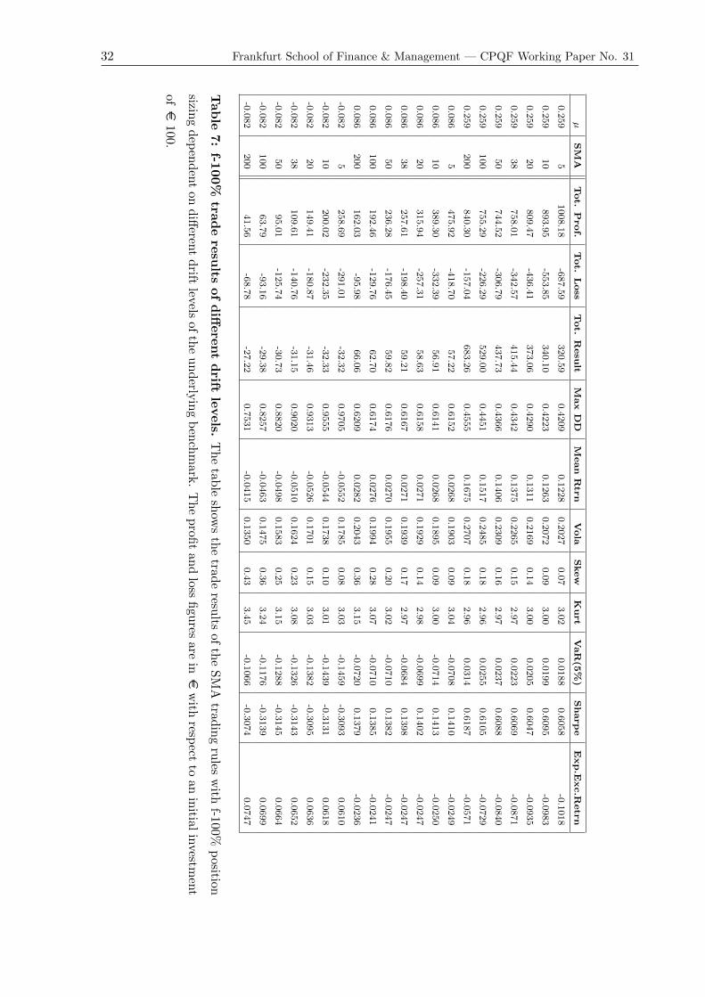
32 Frankfurt School of Finance & Management — CPQF Working Paper No. 31
µSM
ATot.
Prof.
Tot.
Loss
Tot.
Resu
ltM
ax
DD
Mean
Rtrn
Vola
Skew
Kurt
VaR(5
%)
Sharpe
Exp.E
xc.R
etrn
0.259
51008.18
-687.59
320.59
0.4209
0.1228
0.2027
0.07
3.02
0.0188
0.6058
-0.1018
0.259
10
893.95
-553.85
340.10
0.4223
0.1263
0.2072
0.09
3.00
0.0199
0.6095
-0.0983
0.259
20
809.47
-436.41
373.06
0.4290
0.1311
0.2169
0.14
3.00
0.0205
0.6047
-0.0935
0.259
38
758.01
-342.57
415.44
0.4342
0.1375
0.2265
0.15
2.97
0.0223
0.6069
-0.0871
0.259
50
744.52
-306.79
437.73
0.4366
0.1406
0.2309
0.16
2.97
0.0237
0.6088
-0.0840
0.259
100
755.29
-226.29
529.00
0.4451
0.1517
0.2485
0.18
2.96
0.0255
0.6105
-0.0729
0.259
200
840.30
-157.04
683.26
0.4555
0.1675
0.2707
0.18
2.96
0.0314
0.6187
-0.0571
0.086
5475.92
-418.70
57.22
0.6152
0.0268
0.1903
0.09
3.04
-0.0708
0.1410
-0.0249
0.086
10
389.30
-332.39
56.91
0.6141
0.0268
0.1895
0.09
3.00
-0.0714
0.1413
-0.0250
0.086
20
315.94
-257.31
58.63
0.6158
0.0271
0.1929
0.14
2.98
-0.0699
0.1402
-0.0247
0.086
38
257.61
-198.40
59.21
0.6167
0.0271
0.1939
0.17
2.97
-0.0684
0.1398
-0.0247
0.086
50
236.28
-176.45
59.82
0.6176
0.0270
0.1955
0.20
3.02
-0.0710
0.1382
-0.0247
0.086
100
192.46
-129.76
62.70
0.6174
0.0276
0.1994
0.28
3.07
-0.0710
0.1385
-0.0241
0.086
200
162.03
-95.98
66.06
0.6209
0.0282
0.2043
0.36
3.15
-0.0720
0.1379
-0.0236
-0.082
5258.69
-291.01
-32.32
0.9705
-0.0552
0.1785
0.08
3.03
-0.1459
-0.3093
0.0610
-0.082
10
200.02
-232.35
-32.33
0.9555
-0.0544
0.1738
0.10
3.01
-0.1439
-0.3131
0.0618
-0.082
20
149.41
-180.87
-31.46
0.9313
-0.0526
0.1701
0.15
3.03
-0.1382
-0.3095
0.0636
-0.082
38
109.61
-140.76
-31.15
0.9020
-0.0510
0.1624
0.23
3.08
-0.1326
-0.3143
0.0652
-0.082
50
95.01
-125.74
-30.73
0.8820
-0.0498
0.1583
0.25
3.15
-0.1288
-0.3145
0.0664
-0.082
100
63.79
-93.16
-29.38
0.8257
-0.0463
0.1475
0.36
3.24
-0.1176
-0.3139
0.0699
-0.082
200
41.56
-68.78
-27.22
0.7531
-0.0415
0.1350
0.43
3.45
-0.1066
-0.3074
0.0747
Tab
le7:
f-100%
trad
ere
sults
of
diff
ere
nt
drift
levels.
Th
etab
lesh
ows
the
trade
results
ofth
eS
MA
tradin
gru
lesw
ithf-100%
position
sizing
dep
end
ent
on
diff
erent
drift
levelsof
the
und
erlyin
gb
ench
mark
.T
he
profi
tan
dloss
figu
resare
ine
with
respect
toan
initial
investm
ent
ofe
100.

Frankfurt School of Finance & Management — CPQF Working Paper No. 31 33
µSM
ATot.
Prof.
Tot.
Loss
Tot.
Resu
ltM
ax
DD
Mean
Rtrn
Vola
Skew
Kurt
VaR(5
%)
Sharpe
Exp.E
xc.R
etrn
0.259
51563.71
-1065.28
498.43
0.5319
0.1469
0.2509
0.07
3.01
0.0180
0.5853
-0.0778
0.259
10
1389.53
-860.16
529.37
0.5323
0.1506
0.2553
0.09
2.99
0.0195
0.5899
-0.0740
0.259
20
1263.82
-680.28
583.53
0.5387
0.1558
0.2654
0.13
3.00
0.0197
0.5869
-0.0689
0.259
38
1183.40
-534.80
648.60
0.5425
0.1624
0.2746
0.13
2.96
0.0225
0.5913
-0.0622
0.259
50
1160.36
-478.85
681.51
0.5440
0.1655
0.2784
0.13
2.96
0.0240
0.5946
-0.0591
0.259
100
1164.54
-350.62
813.92
0.5492
0.1766
0.2938
0.13
2.94
0.0259
0.6012
-0.0480
0.259
200
1254.57
-237.96
1016.61
0.5533
0.1919
0.3109
0.10
2.91
0.0335
0.6172
-0.0327
0.086
5629.30
-553.27
76.03
0.7823
0.0281
0.2360
0.08
3.04
-0.0929
0.1191
-0.0236
0.086
10
513.09
-438.01
75.08
0.7789
0.0280
0.2343
0.08
3.00
-0.0933
0.1196
-0.0237
0.086
20
415.75
-338.37
77.39
0.7781
0.0283
0.2374
0.13
2.97
-0.0912
0.1193
-0.0234
0.086
38
337.50
-259.91
77.59
0.7757
0.0283
0.2371
0.15
2.96
-0.0888
0.1194
-0.0234
0.086
50
309.11
-230.76
78.36
0.7753
0.0282
0.2385
0.17
3.01
-0.0918
0.1182
-0.0236
0.086
100
250.20
-168.61
81.59
0.7697
0.0289
0.2410
0.24
3.04
-0.0912
0.1197
-0.0229
0.086
200
208.15
-123.48
84.67
0.7672
0.0293
0.2438
0.30
3.08
-0.0919
0.1201
-0.0225
-0.082
5308.29
-346.72
-38.43
1.2370
-0.0735
0.2217
0.08
3.03
-0.1861
-0.3316
0.0427
-0.082
10
238.06
-276.52
-38.46
1.2149
-0.0723
0.2154
0.10
3.01
-0.1833
-0.3354
0.0440
-0.082
20
177.80
-215.18
-37.38
1.1800
-0.0696
0.2102
0.15
3.02
-0.1753
-0.3312
0.0466
-0.082
38
130.39
-167.40
-37.00
1.1384
-0.0671
0.2000
0.21
3.07
-0.1682
-0.3357
0.0491
-0.082
50
112.95
-149.48
-36.53
1.1111
-0.0654
0.1947
0.23
3.13
-0.1627
-0.3357
0.0509
-0.082
100
75.78
-110.69
-34.91
1.0346
-0.0604
0.1808
0.33
3.20
-0.1483
-0.3340
0.0558
-0.082
200
49.42
-81.82
-32.40
0.9383
-0.0537
0.1649
0.38
3.37
-0.1341
-0.3259
0.0625
Tab
le8:
f-125%
trad
ere
sult
sof
diff
ere
nt
dri
ftle
vels
.T
he
tab
lesh
ows
the
trad
ere
sult
sof
the
SM
Atr
ad
ing
rule
sw
ith
f-125
%p
osit
ion
sizi
ng
dep
end
ent
ond
iffer
ent
dri
ftle
vels
ofth
eun
der
lyin
gb
ench
mar
k.
Th
ep
rofi
tan
dlo
ssfi
gure
sar
eine
wit
hre
spec
tto
anin
itia
lin
vest
men
t
ofe
100
.

34 Frankfurt School of Finance & Management — CPQF Working Paper No. 31
µSM
ATot.
Prof.
Tot.
Loss
Tot.
Resu
ltM
ax
DD
Mean
Rtrn
Vola
Skew
Kurt
VaR(5
%)
Sharpe
Exp.E
xc.R
etrn
0.259
52159.46
-1470.79
688.67
0.8221
0.1442
0.6041
-4.44
27.06
-0.0006
0.2388
-0.0804
0.259
10
1869.79
-1156.94
712.85
0.7835
0.1523
0.5547
-4.72
32.13
0.0113
0.2745
-0.0723
0.259
20
1628.97
-877.74
751.23
0.7647
0.1593
0.5168
-4.76
34.70
0.0135
0.3082
-0.0653
0.259
38
1451.60
-657.33
794.26
0.7339
0.1674
0.4740
-4.77
38.02
0.0206
0.3532
-0.0572
0.259
50
1391.14
-575.09
816.05
0.7257
0.1693
0.4810
-4.79
37.69
0.0222
0.3519
-0.0554
0.259
100
1281.59
-386.87
894.72
0.6811
0.1795
0.4437
-4.84
43.84
0.0293
0.4046
-0.0451
0.259
200
1227.34
-236.33
991.01
0.6303
0.1909
0.4009
-4.26
41.82
0.0378
0.4762
-0.0337
0.086
5600.61
-528.46
72.15
0.9290
-0.0046
0.6620
-4.47
24.45
-0.1308
-0.0069
-0.0563
0.086
10
493.86
-421.35
72.51
0.9229
-0.0023
0.6394
-4.56
25.67
-0.1301
-0.0037
-0.0541
0.086
20
401.42
-326.78
74.64
0.9195
0.0005
0.6196
-4.71
27.85
-0.1240
0.0007
-0.0513
0.086
38
329.26
-253.44
75.82
0.9177
0.0012
0.6138
-4.73
28.23
-0.1266
0.0019
-0.0506
0.086
50
302.55
-226.14
76.41
0.9242
-0.0004
0.6340
-4.72
27.95
-0.1337
-0.0006
-0.0522
0.086
100
247.47
-167.10
80.36
0.9188
-0.0004
0.6447
-4.61
26.70
-0.1325
-0.0006
-0.0521
0.086
200
207.99
-123.39
84.59
0.8977
0.0054
0.5960
-4.81
30.10
-0.1200
0.0090
-0.0464
-0.082
5215.16
-242.28
-27.12
0.8842
-0.0625
0.5013
-6.28
46.42
-0.1602
-0.1247
0.0537
-0.082
10
167.48
-194.68
-27.20
0.8689
-0.0613
0.4881
-6.37
47.65
-0.1557
-0.1257
0.0549
-0.082
20
125.45
-152.16
-26.71
0.8547
-0.0605
0.4905
-6.42
48.36
-0.1518
-0.1233
0.0558
-0.082
38
92.71
-119.09
-26.38
0.8253
-0.0558
0.4378
-7.06
59.72
-0.1443
-0.1275
0.0604
-0.082
50
80.61
-106.68
-26.07
0.8123
-0.0575
0.4771
-6.85
54.90
-0.1416
-0.1205
0.0588
-0.082
100
54.96
-80.54
-25.58
0.7848
-0.0536
0.4323
-7.21
62.44
-0.1421
-0.1240
0.0626
-0.082
200
36.81
-61.11
-24.30
0.7402
-0.0514
0.4341
-7.18
60.53
-0.1377
-0.1185
0.0648
Tab
le9:
Un
sized
trad
ere
sults
of
diff
ere
nt
drift
levels.
Th
etab
lesh
ows
the
trade
results
ofth
eS
MA
tradin
gru
lesw
ithu
nm
anaged
position
sizing
dep
end
ent
ond
ifferen
td
riftlevels
ofth
eu
nd
erlyin
gb
ench
mark
.T
he
profi
tan
dloss
figu
resare
ine
with
respect
toan
initial
investm
ent
ofe
100.

Frankfurt School of Finance & Management — CPQF Working Paper No. 31 35
σSM
ATot.
Prof.
Tot.
Loss
Tot.
Resu
ltM
ax
DD
Mean
Rtrn
Vola
Skew
Kurt
VaR(5
%)
Sharpe
Exp.E
xc.R
etrn
0.39
5155.25
-137.08
18.17
0.2249
0.0140
0.0737
0.10
3.04
-0.0237
0.1896
-0.0353
0.39
10
127.79
-109.38
18.40
0.2268
0.0141
0.0747
0.14
3.04
-0.0240
0.1886
-0.0352
0.39
20
104.10
-85.14
18.96
0.2312
0.0143
0.0775
0.20
3.05
-0.0246
0.1847
-0.0349
0.39
38
85.85
-66.29
19.56
0.2364
0.0146
0.0805
0.29
3.13
-0.0249
0.1808
-0.0347
0.39
50
79.14
-59.23
19.91
0.2395
0.0147
0.0824
0.35
3.27
-0.0256
0.1778
-0.0346
0.39
100
65.65
-44.38
21.27
0.2493
0.0151
0.0888
0.55
3.64
-0.0267
0.1705
-0.0341
0.39
200
57.66
-33.74
23.92
0.2653
0.0161
0.0987
0.90
4.61
-0.0269
0.1627
-0.0332
0.26
5100.95
-88.96
12.00
0.1464
0.0101
0.0489
0.10
3.04
-0.0148
0.2075
-0.0416
0.26
10
83.13
-71.02
12.12
0.1473
0.0102
0.0493
0.11
3.02
-0.0152
0.2075
-0.0415
0.26
20
67.72
-55.26
12.46
0.1495
0.0104
0.0510
0.18
3.01
-0.0152
0.2044
-0.0413
0.26
38
55.80
-43.01
12.80
0.1522
0.0106
0.0526
0.25
3.06
-0.0150
0.2023
-0.0411
0.26
50
51.41
-38.44
12.96
0.1537
0.0107
0.0538
0.30
3.16
-0.0157
0.1995
-0.0410
0.26
100
42.54
-28.74
13.80
0.1582
0.0112
0.0575
0.47
3.41
-0.0162
0.1955
-0.0405
0.26
200
36.94
-21.79
15.16
0.1664
0.0120
0.0634
0.76
4.21
-0.0169
0.1895
-0.0397
0.16
562.25
-53.64
8.61
0.0856
0.0078
0.0301
0.09
3.05
-0.0075
0.2594
-0.0419
0.16
10
51.53
-42.80
8.73
0.0859
0.0079
0.0304
0.11
3.01
-0.0076
0.2606
-0.0418
0.16
20
42.24
-33.27
8.97
0.0870
0.0081
0.0313
0.16
2.98
-0.0078
0.2586
-0.0416
0.16
38
35.09
-25.86
9.23
0.0884
0.0083
0.0324
0.22
3.03
-0.0077
0.2567
-0.0414
0.16
50
32.47
-23.07
9.40
0.0890
0.0084
0.0331
0.24
3.08
-0.0081
0.2552
-0.0413
0.16
100
27.14
-17.22
9.92
0.0914
0.0088
0.0353
0.39
3.20
-0.0083
0.2506
-0.0409
0.16
200
23.81
-12.98
10.83
0.0957
0.0095
0.0388
0.57
3.62
-0.0087
0.2457
-0.0402
Tab
le10:
f-25%
trad
ere
sult
sof
diff
ere
nt
vola
tility
levels
.T
he
tab
lesh
ows
the
trad
ere
sult
sof
the
SM
Atr
adin
gru
les
wit
hf-
25%
posi
tion
sizi
ng
dep
end
ent
on
diff
eren
tvo
lati
lity
leve
lsof
the
un
der
lyin
gb
ench
mar
k.
Th
ep
rofit
and
loss
figu
res
are
ine
wit
hre
spec
tto
an
init
ial
inves
tmen
tofe
100
.

36 Frankfurt School of Finance & Management — CPQF Working Paper No. 31
σSM
ATot.
Prof.
Tot.
Loss
Tot.
Resu
ltM
ax
DD
Mean
Rtrn
Vola
Skew
Kurt
VaR(5
%)
Sharpe
Exp.E
xc.R
etrn
0.39
5336.42
-296.83
39.59
0.4609
0.0227
0.1452
0.09
3.04
-0.0518
0.1561
-0.0266
0.39
10
276.24
-236.35
39.89
0.4627
0.0227
0.1462
0.12
3.03
-0.0520
0.1552
-0.0266
0.39
20
224.60
-183.49
41.11
0.4685
0.0229
0.1502
0.17
3.02
-0.0527
0.1523
-0.0264
0.39
38
184.44
-142.33
42.10
0.4746
0.0229
0.1535
0.24
3.06
-0.0532
0.1493
-0.0264
0.39
50
169.66
-126.85
42.81
0.4785
0.0229
0.1558
0.28
3.13
-0.0541
0.1470
-0.0264
0.39
100
139.65
-94.28
45.37
0.4889
0.0231
0.1629
0.41
3.28
-0.0556
0.1420
-0.0261
0.39
200
121.06
-70.97
50.09
0.5046
0.0237
0.1728
0.62
3.64
-0.0554
0.1375
-0.0255
0.26
5213.11
-187.70
25.41
0.2976
0.0179
0.0968
0.09
3.04
-0.0315
0.1851
-0.0338
0.26
10
175.19
-149.62
25.56
0.2986
0.0180
0.0972
0.11
3.01
-0.0322
0.1852
-0.0338
0.26
20
142.55
-116.25
26.30
0.3018
0.0183
0.1000
0.16
2.99
-0.0320
0.1828
-0.0335
0.26
38
117.10
-90.22
26.88
0.3053
0.0185
0.1020
0.22
3.02
-0.0315
0.1813
-0.0333
0.26
50
107.72
-80.52
27.20
0.3073
0.0185
0.1037
0.25
3.09
-0.0328
0.1789
-0.0332
0.26
100
88.73
-59.89
28.83
0.3126
0.0192
0.1086
0.38
3.21
-0.0334
0.1767
-0.0326
0.26
200
76.33
-45.08
31.25
0.3222
0.0200
0.1156
0.55
3.54
-0.0346
0.1733
-0.0317
0.16
5129.52
-111.58
17.94
0.1728
0.0147
0.0599
0.09
3.05
-0.0157
0.2456
-0.0350
0.16
10
107.13
-88.97
18.16
0.1732
0.0149
0.0602
0.10
3.00
-0.0160
0.2469
-0.0348
0.16
20
87.76
-69.10
18.66
0.1750
0.0152
0.0619
0.15
2.97
-0.0163
0.2453
-0.0345
0.16
38
72.79
-53.64
19.15
0.1770
0.0155
0.0635
0.20
3.00
-0.0159
0.2439
-0.0342
0.16
50
67.31
-47.81
19.50
0.1779
0.0157
0.0647
0.21
3.05
-0.0168
0.2428
-0.0340
0.16
100
56.08
-35.58
20.51
0.1814
0.0163
0.0680
0.34
3.11
-0.0172
0.2395
-0.0334
0.16
200
48.91
-26.69
22.22
0.1876
0.0173
0.0731
0.46
3.33
-0.0178
0.2369
-0.0324
Tab
le11:
f-50%
trad
ere
sults
of
diff
ere
nt
vola
tilityle
vels.
Th
etab
lesh
ows
the
trade
results
ofth
eS
MA
tradin
gru
lesw
ithf-50%
position
sizing
dep
end
ent
ond
ifferen
tvo
latilitylevels
ofth
eu
nd
erlyin
gb
ench
mark
.T
he
profi
tan
dloss
figu
resare
ine
with
respect
toan
initia
lin
vestm
ent
ofe
100.
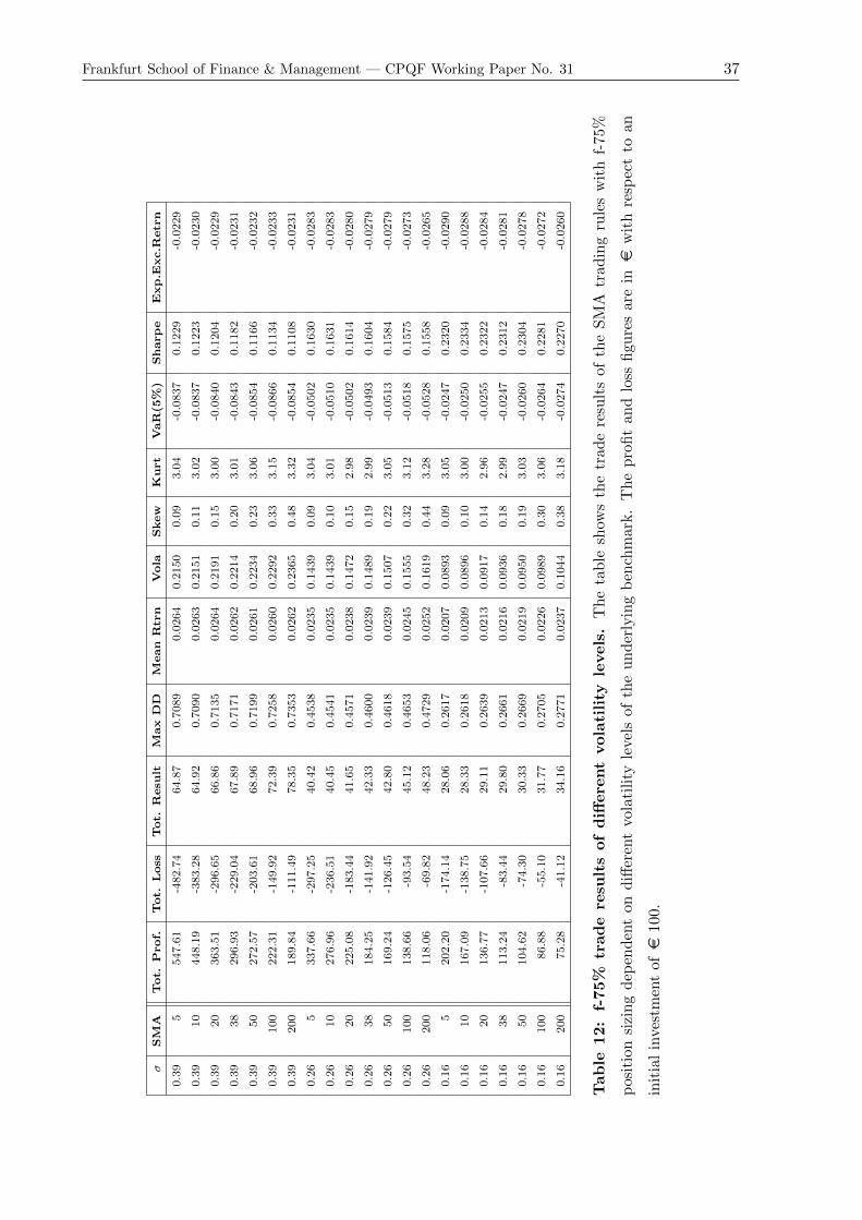
Frankfurt School of Finance & Management — CPQF Working Paper No. 31 37
σSM
ATot.
Prof.
Tot.
Loss
Tot.
Resu
ltM
ax
DD
Mean
Rtrn
Vola
Skew
Kurt
VaR(5
%)
Sharpe
Exp.E
xc.R
etrn
0.39
5547.61
-482.74
64.87
0.7089
0.0264
0.2150
0.09
3.04
-0.0837
0.1229
-0.0229
0.39
10
448.19
-383.28
64.92
0.7090
0.0263
0.2151
0.11
3.02
-0.0837
0.1223
-0.0230
0.39
20
363.51
-296.65
66.86
0.7135
0.0264
0.2191
0.15
3.00
-0.0840
0.1204
-0.0229
0.39
38
296.93
-229.04
67.89
0.7171
0.0262
0.2214
0.20
3.01
-0.0843
0.1182
-0.0231
0.39
50
272.57
-203.61
68.96
0.7199
0.0261
0.2234
0.23
3.06
-0.0854
0.1166
-0.0232
0.39
100
222.31
-149.92
72.39
0.7258
0.0260
0.2292
0.33
3.15
-0.0866
0.1134
-0.0233
0.39
200
189.84
-111.49
78.35
0.7353
0.0262
0.2365
0.48
3.32
-0.0854
0.1108
-0.0231
0.26
5337.66
-297.25
40.42
0.4538
0.0235
0.1439
0.09
3.04
-0.0502
0.1630
-0.0283
0.26
10
276.96
-236.51
40.45
0.4541
0.0235
0.1439
0.10
3.01
-0.0510
0.1631
-0.0283
0.26
20
225.08
-183.44
41.65
0.4571
0.0238
0.1472
0.15
2.98
-0.0502
0.1614
-0.0280
0.26
38
184.25
-141.92
42.33
0.4600
0.0239
0.1489
0.19
2.99
-0.0493
0.1604
-0.0279
0.26
50
169.24
-126.45
42.80
0.4618
0.0239
0.1507
0.22
3.05
-0.0513
0.1584
-0.0279
0.26
100
138.66
-93.54
45.12
0.4653
0.0245
0.1555
0.32
3.12
-0.0518
0.1575
-0.0273
0.26
200
118.06
-69.82
48.23
0.4729
0.0252
0.1619
0.44
3.28
-0.0528
0.1558
-0.0265
0.16
5202.20
-174.14
28.06
0.2617
0.0207
0.0893
0.09
3.05
-0.0247
0.2320
-0.0290
0.16
10
167.09
-138.75
28.33
0.2618
0.0209
0.0896
0.10
3.00
-0.0250
0.2334
-0.0288
0.16
20
136.77
-107.66
29.11
0.2639
0.0213
0.0917
0.14
2.96
-0.0255
0.2322
-0.0284
0.16
38
113.24
-83.44
29.80
0.2661
0.0216
0.0936
0.18
2.99
-0.0247
0.2312
-0.0281
0.16
50
104.62
-74.30
30.33
0.2669
0.0219
0.0950
0.19
3.03
-0.0260
0.2304
-0.0278
0.16
100
86.88
-55.10
31.77
0.2705
0.0226
0.0989
0.30
3.06
-0.0264
0.2281
-0.0272
0.16
200
75.28
-41.12
34.16
0.2771
0.0237
0.1044
0.38
3.18
-0.0274
0.2270
-0.0260
Tab
le12:
f-75%
trad
ere
sult
sof
diff
ere
nt
vola
tility
levels
.T
he
tab
lesh
ows
the
trad
ere
sult
sof
the
SM
Atr
adin
gru
les
wit
hf-
75%
posi
tion
sizi
ng
dep
end
ent
on
diff
eren
tvo
lati
lity
leve
lsof
the
un
der
lyin
gb
ench
mar
k.
Th
ep
rofit
and
loss
figu
res
are
ine
wit
hre
spec
tto
an
init
ial
inves
tmen
tofe
100
.

38 Frankfurt School of Finance & Management — CPQF Working Paper No. 31
σSM
ATot.
Prof.
Tot.
Loss
Tot.
Resu
ltM
ax
DD
Mean
Rtrn
Vola
Skew
Kurt
VaR(5
%)
Sharpe
Exp.E
xc.R
etrn
0.39
5793.47
-698.72
94.76
0.9698
0.0255
0.2832
0.08
3.04
-0.1196
0.0900
-0.0238
0.39
10
646.72
-552.76
93.96
0.9664
0.0253
0.2819
0.10
3.01
-0.1190
0.0898
-0.0239
0.39
20
522.88
-426.22
96.66
0.9671
0.0254
0.2852
0.13
2.99
-0.1193
0.0890
-0.0239
0.39
38
424.42
-327.30
97.12
0.9651
0.0251
0.2856
0.17
2.99
-0.1181
0.0877
-0.0242
0.39
50
388.83
-290.21
98.61
0.9654
0.0249
0.2869
0.20
3.03
-0.1190
0.0868
-0.0244
0.39
100
313.85
-211.51
102.34
0.9628
0.0248
0.2904
0.27
3.08
-0.1195
0.0853
-0.0245
0.39
200
263.60
-155.07
108.53
0.9625
0.0248
0.2942
0.39
3.17
-0.1168
0.0842
-0.0245
0.26
5475.92
-418.70
57.22
0.6152
0.0268
0.1903
0.09
3.04
-0.0708
0.1410
-0.0249
0.26
10
389.30
-332.39
56.91
0.6141
0.0268
0.1895
0.09
3.00
-0.0714
0.1413
-0.0250
0.26
20
315.94
-257.31
58.63
0.6158
0.0271
0.1929
0.14
2.98
-0.0699
0.1402
-0.0247
0.26
38
257.61
-198.40
59.21
0.6167
0.0271
0.1939
0.17
2.97
-0.0684
0.1398
-0.0247
0.26
50
236.28
-176.45
59.82
0.6176
0.0270
0.1955
0.20
3.02
-0.0710
0.1382
-0.0247
0.26
100
192.46
-129.76
62.70
0.6174
0.0276
0.1994
0.28
3.07
-0.0710
0.1385
-0.0241
0.26
200
162.03
-95.98
66.06
0.6209
0.0282
0.2043
0.36
3.15
-0.0720
0.1379
-0.0236
0.16
5280.71
-241.68
39.04
0.3523
0.0259
0.1184
0.09
3.05
-0.0343
0.2185
-0.0238
0.16
10
231.69
-192.38
39.31
0.3519
0.0261
0.1185
0.09
3.00
-0.0348
0.2199
-0.0237
0.16
20
189.48
-149.10
40.38
0.3539
0.0265
0.1209
0.14
2.96
-0.0352
0.2192
-0.0232
0.16
38
156.58
-115.36
41.22
0.3558
0.0268
0.1228
0.16
2.97
-0.0341
0.2185
-0.0229
0.16
50
144.55
-102.62
41.92
0.3563
0.0271
0.1243
0.18
3.01
-0.0357
0.2181
-0.0226
0.16
100
119.58
-75.84
43.75
0.3591
0.0278
0.1282
0.27
3.02
-0.0360
0.2167
-0.0219
0.16
200
102.92
-56.28
46.64
0.3649
0.0289
0.1337
0.32
3.09
-0.0371
0.2166
-0.0208
Tab
le13:
f-100%
trad
ere
sults
of
diff
ere
nt
vola
tilityle
vels.
Th
etab
lesh
ows
the
trade
results
ofth
eS
MA
tradin
gru
lesw
ithf-100%
positio
nsizin
gd
epen
den
ton
diff
erent
volatilitylevels
ofth
eu
nd
erlyin
gb
ench
mark
.T
he
profi
tan
dloss
figu
resare
ine
with
respect
toan
initial
investm
ent
ofe
100.

Frankfurt School of Finance & Management — CPQF Working Paper No. 31 39
σSM
ATot.
Prof.
Tot.
Loss
Tot.
Resu
ltM
ax
DD
Mean
Rtrn
Vola
Skew
Kurt
VaR(5
%)
Sharpe
Exp.E
xc.R
etrn
0.39
51079.28
-949.19
130.09
1.2446
0.0201
0.3502
0.08
3.03
-0.1591
0.0575
-0.0291
0.39
10
875.02
-747.53
127.50
1.2358
0.0200
0.3470
0.09
3.01
-0.1579
0.0578
-0.0292
0.39
20
704.74
-573.82
130.91
1.2302
0.0203
0.3490
0.12
2.98
-0.1570
0.0581
-0.0290
0.39
38
567.87
-437.89
129.97
1.2197
0.0201
0.3469
0.15
2.97
-0.1544
0.0579
-0.0292
0.39
50
519.39
-387.37
132.02
1.2163
0.0200
0.3473
0.17
3.00
-0.1552
0.0577
-0.0292
0.39
100
414.40
-279.20
135.20
1.2019
0.0202
0.3479
0.23
3.04
-0.1542
0.0580
-0.0291
0.39
200
341.90
-201.49
140.41
1.1887
0.0203
0.3477
0.32
3.09
-0.1494
0.0584
-0.0290
0.26
5629.30
-553.27
76.03
0.7823
0.0281
0.2360
0.08
3.04
-0.0929
0.1191
-0.0236
0.26
10
513.09
-438.01
75.08
0.7789
0.0280
0.2343
0.08
3.00
-0.0933
0.1196
-0.0237
0.26
20
415.75
-338.37
77.39
0.7781
0.0283
0.2374
0.13
2.97
-0.0912
0.1193
-0.0234
0.26
38
337.50
-259.91
77.59
0.7757
0.0283
0.2371
0.15
2.96
-0.0888
0.1194
-0.0234
0.26
50
309.11
-230.76
78.36
0.7753
0.0282
0.2385
0.17
3.01
-0.0918
0.1182
-0.0236
0.26
100
250.20
-168.61
81.59
0.7697
0.0289
0.2410
0.24
3.04
-0.0912
0.1197
-0.0229
0.26
200
208.15
-123.48
84.67
0.7672
0.0293
0.2438
0.30
3.08
-0.0919
0.1201
-0.0225
0.16
5365.51
-314.56
50.95
0.4447
0.0302
0.1473
0.08
3.05
-0.0448
0.2050
-0.0195
0.16
10
301.27
-250.12
51.15
0.4435
0.0304
0.1470
0.09
2.99
-0.0451
0.2066
-0.0193
0.16
20
246.13
-193.62
52.51
0.4450
0.0308
0.1495
0.13
2.96
-0.0456
0.2062
-0.0189
0.16
38
202.95
-149.52
53.43
0.4461
0.0311
0.1511
0.15
2.96
-0.0440
0.2060
-0.0186
0.16
50
187.21
-132.88
54.33
0.4460
0.0314
0.1527
0.16
3.00
-0.0459
0.2058
-0.0183
0.16
100
154.26
-97.82
56.44
0.4473
0.0321
0.1563
0.24
3.00
-0.0462
0.2052
-0.0176
0.16
200
131.81
-72.15
59.66
0.4515
0.0332
0.1612
0.28
3.04
-0.0473
0.2059
-0.0165
Tab
le14:
f-125%
trad
ere
sult
sof
diff
ere
nt
vola
tility
levels
.T
he
tab
lesh
ows
the
trad
ere
sult
sof
the
SM
Atr
ad
ing
rule
sw
ith
f-25%
posi
tion
sizi
ng
dep
end
ent
on
diff
eren
tvo
lati
lity
leve
lsof
the
un
der
lyin
gb
ench
mar
k.
Th
ep
rofit
and
loss
figu
res
are
ine
wit
hre
spec
tto
an
init
ial
inves
tmen
tofe
100
.

40 Frankfurt School of Finance & Management — CPQF Working Paper No. 31
σSM
ATot.
Prof.
Tot.
Loss
Tot.
Resu
ltM
ax
DD
Mean
Rtrn
Vola
Skew
Kurt
VaR(5
%)
Sharpe
Exp.E
xc.R
etrn
0.39
51130.35
-995.49
134.86
1.7440
-0.1261
1.2656
-1.70
4.45
-1.0641
-0.0996
-0.1753
0.39
10
928.60
-793.09
135.51
1.7213
-0.1181
1.2388
-1.77
4.76
-1.0530
-0.0954
-0.1674
0.39
20
754.43
-614.55
139.88
1.7382
-0.1167
1.2396
-1.79
4.82
-1.0600
-0.0941
-0.1659
0.39
38
618.04
-476.03
142.02
1.7596
-0.1230
1.2631
-1.73
4.61
-1.0637
-0.0974
-0.1723
0.39
50
567.49
-423.97
143.52
1.7524
-0.1233
1.2628
-1.73
4.58
-1.0594
-0.0976
-0.1726
0.39
100
463.28
-312.00
151.29
1.7480
-0.1189
1.2556
-1.76
4.75
-1.0594
-0.0947
-0.1681
0.39
200
387.92
-228.89
159.03
1.7247
-0.1089
1.2214
-1.84
5.14
-1.0526
-0.0892
-0.1582
0.26
5600.61
-528.46
72.15
0.9290
-0.0046
0.6620
-4.47
24.45
-0.1308
-0.0069
-0.0563
0.26
10
493.86
-421.35
72.51
0.9229
-0.0023
0.6394
-4.56
25.67
-0.1301
-0.0037
-0.0541
0.26
20
401.42
-326.78
74.64
0.9195
0.0005
0.6196
-4.71
27.85
-0.1240
0.0007
-0.0513
0.26
38
329.26
-253.44
75.82
0.9177
0.0012
0.6138
-4.73
28.23
-0.1266
0.0019
-0.0506
0.26
50
302.55
-226.14
76.41
0.9242
-0.0004
0.6340
-4.72
27.95
-0.1337
-0.0006
-0.0522
0.26
100
247.47
-167.10
80.36
0.9188
-0.0004
0.6447
-4.61
26.70
-0.1325
-0.0006
-0.0521
0.26
200
207.99
-123.39
84.59
0.8977
0.0054
0.5960
-4.81
30.10
-0.1200
0.0090
-0.0464
0.16
5331.04
-285.03
46.00
0.4263
0.0276
0.1606
-6.52
184.51
-0.0436
0.1720
-0.0221
0.16
10
273.68
-227.14
46.54
0.4235
0.0280
0.1581
-4.84
112.00
-0.0433
0.1771
-0.0217
0.16
20
223.89
-176.12
47.77
0.4244
0.0285
0.1586
-4.74
118.88
-0.0432
0.1800
-0.0212
0.16
38
185.30
-136.52
48.78
0.4249
0.0291
0.1493
-1.52
39.06
-0.0424
0.1952
-0.0206
0.16
50
171.08
-121.52
49.57
0.4265
0.0293
0.1581
-3.82
103.84
-0.0437
0.1853
-0.0204
0.16
100
141.60
-89.91
51.69
0.4278
0.0299
0.1681
-5.43
150.12
-0.0445
0.1780
-0.0198
0.16
200
121.08
-66.28
54.80
0.4287
0.0314
0.1593
-1.29
34.88
-0.0450
0.1973
-0.0183
Tab
le15:
Un
sized
trad
ere
sults
of
diff
ere
nt
vola
tilityle
vels.
Th
etab
lesh
ows
the
trade
results
ofth
eS
MA
tradin
gru
lesw
ith
un
man
agedp
ositionsizin
gd
epen
den
ton
diff
erent
volatilitylevels
ofth
eu
nd
erlyin
gb
ench
mark
.T
he
profi
tan
dloss
figu
resare
ine
with
respect
toan
initia
lin
vestmen
tofe
100.

Frankfurt School of Finance & Management — CPQF Working Paper No. 31 41
ϕSM
ATot.
Prof.
Tot.
Loss
Tot.
Resu
ltM
ax
DD
Mean
Rtrn
Vola
Skew
Kurt
VaR(5
%)
Sharpe
Exp.E
xc.R
etrn
0.2
5190.89
-88.50
102.39
0.0688
0.0689
0.0561
0.10
3.03
0.0403
1.2279
0.0175
0.2
10
142.65
-66.52
76.13
0.0798
0.0550
0.0570
0.14
3.04
0.0258
0.9653
0.0035
0.2
20
107.02
-49.45
57.57
0.0934
0.0437
0.0590
0.22
3.06
0.0142
0.7409
-0.0077
0.2
38
83.03
-37.38
45.64
0.1073
0.0357
0.0612
0.31
3.13
0.0058
0.5831
-0.0158
0.2
50
74.85
-33.09
41.76
0.1135
0.0329
0.0625
0.38
3.27
0.0024
0.5269
-0.0185
0.2
100
59.21
-24.35
34.86
0.1319
0.0275
0.0673
0.58
3.63
-0.0038
0.4091
-0.0239
0.2
200
49.88
-18.49
31.38
0.1543
0.0242
0.0753
0.93
4.64
-0.0086
0.3221
-0.0272
0.025
5109.11
-88.85
20.26
0.1284
0.0172
0.0496
0.10
3.04
-0.0082
0.3471
-0.0345
0.025
10
88.77
-70.41
18.36
0.1334
0.0156
0.0501
0.12
3.03
-0.0102
0.3117
-0.0362
0.025
20
71.60
-54.50
17.11
0.1390
0.0144
0.0518
0.18
3.02
-0.0116
0.2790
-0.0373
0.025
38
58.56
-42.26
16.30
0.1444
0.0137
0.0535
0.25
3.07
-0.0125
0.2555
-0.0381
0.025
50
53.81
-37.72
16.09
0.1469
0.0134
0.0547
0.30
3.18
-0.0133
0.2453
-0.0384
0.025
100
44.27
-28.15
16.11
0.1539
0.0132
0.0585
0.48
3.44
-0.0146
0.2254
-0.0386
0.025
200
38.29
-21.34
16.95
0.1640
0.0135
0.0646
0.78
4.26
-0.0157
0.2086
-0.0383
-0.1
574.25
-89.77
-15.52
0.2765
-0.0179
0.0464
0.08
3.03
-0.0417
-0.3864
-0.0696
-0.1
10
64.02
-73.65
-9.63
0.2367
-0.0112
0.0468
0.10
3.02
-0.0354
-0.2397
-0.0629
-0.1
20
54.29
-58.57
-4.29
0.2094
-0.0055
0.0483
0.16
3.01
-0.0300
-0.1148
-0.0573
-0.1
38
46.14
-46.22
-0.07
0.1926
-0.0013
0.0498
0.22
3.04
-0.0261
-0.0265
-0.0530
-0.1
50
43.00
-41.49
1.50
0.1882
0.0002
0.0510
0.25
3.12
-0.0250
0.0036
-0.0515
-0.1
100
36.41
-31.31
5.09
0.1803
0.0035
0.0543
0.40
3.31
-0.0229
0.0640
-0.0482
-0.1
200
32.18
-23.73
8.44
0.1791
0.0063
0.0594
0.66
3.97
-0.0214
0.1055
-0.0454
Tab
le16:
f-25%
trad
ere
sult
sof
diff
ere
nt
au
tocorr
ela
tion
levels
.T
he
tab
lesh
ows
the
trad
ere
sult
sof
the
SM
Atr
adin
gru
les
wit
h
f-25%
pos
itio
nsi
zin
gd
epen
den
ton
diff
eren
tla
g-1
auto
corr
elat
ion
leve
lsof
the
un
der
lyin
gb
ench
mar
k.
Th
ep
rofi
tan
dlo
ssfi
gure
sare
ine
wit
h
resp
ect
toan
init
ial
inve
stm
ent
ofe
100
.
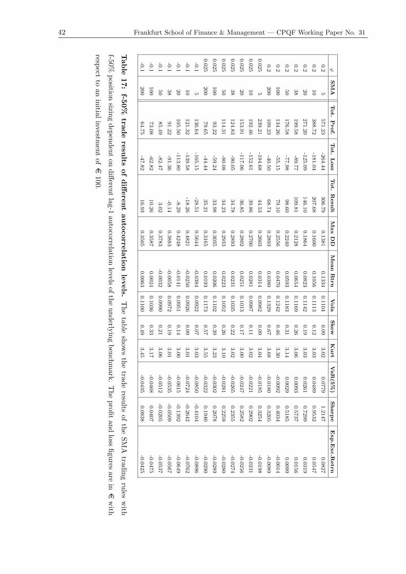
42 Frankfurt School of Finance & Management — CPQF Working Paper No. 31
ϕSM
ATot.
Prof.
Tot.
Loss
Tot.
Resu
ltM
ax
DD
Mean
Rtrn
Vola
Skew
Kurt
VaR(5
%)
Sharpe
Exp.E
xc.R
etrn
0.2
5571.23
-264.44
306.79
0.1381
0.1334
0.1104
0.09
3.02
0.0779
1.2147
0.0827
0.2
10
388.72
-181.04
207.68
0.1600
0.1056
0.1113
0.12
3.03
0.0489
0.9532
0.0547
0.2
20
271.20
-125.09
146.10
0.1864
0.0823
0.1142
0.19
3.03
0.0261
0.7299
0.0319
0.2
38
199.58
-89.77
109.81
0.2128
0.0654
0.1169
0.26
3.06
0.0093
0.5737
0.0156
0.2
50
176.58
-77.98
98.60
0.2240
0.0593
0.1183
0.31
3.14
0.0029
0.5185
0.0099
0.2
100
134.26
-55.15
79.10
0.2556
0.0470
0.1242
0.46
3.30
-0.0092
0.4034
-0.0014
0.2
200
109.23
-40.50
68.74
0.2893
0.0380
0.1329
0.67
3.68
-0.0180
0.3205
-0.0089
0.025
5239.21
-194.68
44.53
0.2603
0.0314
0.0982
0.09
3.04
-0.0185
0.3254
-0.0198
0.025
10
192.46
-152.61
39.86
0.2700
0.0281
0.0987
0.11
3.02
-0.0221
0.2902
-0.0231
0.025
20
153.91
-117.06
36.85
0.2802
0.0251
0.1013
0.17
3.00
-0.0247
0.2582
-0.0256
0.025
38
124.83
-90.05
34.78
0.2893
0.0231
0.1035
0.22
3.02
-0.0265
0.2355
-0.0274
0.025
50
114.31
-80.08
34.23
0.2933
0.0223
0.1052
0.26
3.10
-0.0281
0.2259
-0.0280
0.025
100
93.22
-59.24
33.98
0.3035
0.0206
0.1102
0.39
3.23
-0.0302
0.2078
-0.0289
0.025
200
79.65
-44.44
35.21
0.3165
0.0193
0.1173
0.57
3.55
-0.0322
0.1940
-0.0290
-0.1
5136.64
-165.15
-28.51
0.5644
-0.0384
0.0922
0.07
3.03
-0.0850
-0.4104
-0.0896
-0.1
10
121.32
-139.58
-18.26
0.4821
-0.0250
0.0926
0.09
3.01
-0.0724
-0.2642
-0.0762
-0.1
20
105.50
-113.80
-8.29
0.4248
-0.0141
0.0951
0.14
3.00
-0.0615
-0.1392
-0.0649
-0.1
38
91.22
-91.36
-0.14
0.3883
-0.0058
0.0972
0.19
3.01
-0.0535
-0.0509
-0.0567
-0.1
50
85.49
-82.47
3.02
0.3783
-0.0032
0.0990
0.21
3.06
-0.0512
-0.0205
-0.0537
-0.1
100
73.08
-62.82
10.26
0.3587
0.0024
0.1036
0.33
3.17
-0.0468
0.0407
-0.0475
-0.1
200
64.75
-47.82
16.93
0.3505
0.0063
0.1100
0.49
3.45
-0.0435
0.0838
-0.0425
Tab
le17:
f-50%
trad
ere
sults
of
diff
ere
nt
au
tocorre
latio
nle
vels.
Th
etab
lesh
ows
the
trade
results
ofth
eS
MA
tradin
gru
lesw
ith
f-50%
positio
nsizin
gd
epen
den
ton
diff
erent
lag-1au
tocorrelation
levelsof
the
un
derly
ing
ben
chm
ark.
Th
ep
rofit
and
lossfigu
resare
ine
with
respect
toan
initial
investm
ent
ofe
100.

Frankfurt School of Finance & Management — CPQF Working Paper No. 31 43
ϕSM
ATot.
Prof.
Tot.
Loss
Tot.
Resu
ltM
ax
DD
Mean
Rtrn
Vola
Skew
Kurt
VaR(5
%)
Sharpe
Exp.E
xc.R
etrn
0.2
51323.89
-611.89
712.01
0.2079
0.1959
0.1632
0.09
3.02
0.1128
1.2009
0.1445
0.2
10
809.80
-376.67
433.14
0.2407
0.1537
0.1635
0.11
3.02
0.0695
0.9402
0.1023
0.2
20
520.87
-239.78
281.09
0.2796
0.1195
0.1665
0.17
3.01
0.0357
0.7176
0.0681
0.2
38
361.50
-162.45
199.05
0.3173
0.0948
0.1685
0.22
3.01
0.0109
0.5625
0.0433
0.2
50
313.40
-138.26
175.14
0.3330
0.0861
0.1696
0.27
3.08
0.0016
0.5077
0.0347
0.2
100
228.23
-93.65
134.58
0.3753
0.0689
0.1747
0.38
3.17
-0.0159
0.3943
0.0174
0.2
200
178.90
-66.33
112.57
0.4162
0.0570
0.1821
0.53
3.35
-0.0284
0.3131
0.0056
0.025
5394.20
-320.62
73.58
0.3960
0.0444
0.1460
0.09
3.04
-0.0307
0.3039
-0.0074
0.025
10
313.33
-248.37
64.96
0.4098
0.0392
0.1459
0.10
3.01
-0.0358
0.2689
-0.0125
0.025
20
248.29
-188.71
59.58
0.4238
0.0354
0.1490
0.15
2.99
-0.0397
0.2376
-0.0164
0.025
38
199.54
-143.90
55.64
0.4354
0.0325
0.1509
0.19
2.99
-0.0419
0.2156
-0.0192
0.025
50
182.11
-127.51
54.60
0.4402
0.0315
0.1526
0.22
3.06
-0.0444
0.2064
-0.0203
0.025
100
147.11
-93.41
53.69
0.4510
0.0299
0.1575
0.33
3.13
-0.0469
0.1897
-0.0219
0.025
200
124.03
-69.30
54.72
0.4636
0.0291
0.1639
0.45
3.28
-0.0493
0.1775
-0.0227
-0.1
5189.12
-228.54
-39.41
0.8636
-0.0596
0.1374
0.07
3.03
-0.1299
-0.4341
-0.1114
-0.1
10
172.65
-198.63
-25.98
0.7364
-0.0397
0.1376
0.08
3.01
-0.1109
-0.2882
-0.0914
-0.1
20
153.84
-165.89
-12.05
0.6463
-0.0229
0.1406
0.13
2.99
-0.0942
-0.1629
-0.0746
-0.1
38
135.26
-135.46
-0.21
0.5877
-0.0106
0.1427
0.17
2.99
-0.0821
-0.0745
-0.0623
-0.1
50
127.47
-122.95
4.53
0.5710
-0.0063
0.1447
0.18
3.03
-0.0787
-0.0437
-0.0580
-0.1
100
109.99
-94.51
15.48
0.5367
0.0027
0.1495
0.28
3.10
-0.0716
0.0182
-0.0490
-0.1
200
97.62
-72.19
25.42
0.5183
0.0097
0.1557
0.39
3.24
-0.0665
0.0625
-0.0420
Tab
le18:
f-75%
trad
ere
sult
sof
diff
ere
nt
au
tocorr
ela
tion
levels
.T
he
tab
lesh
ows
the
trad
ere
sult
sof
the
SM
Atr
adin
gru
les
wit
h
f-75%
pos
itio
nsi
zin
gd
epen
den
ton
diff
eren
tla
g-1
auto
corr
elat
ion
leve
lsof
the
un
der
lyin
gb
ench
mar
k.
Th
ep
rofi
tan
dlo
ssfi
gure
sare
ine
wit
h
resp
ect
toan
init
ial
inve
stm
ent
ofe
100
.

44 Frankfurt School of Finance & Management — CPQF Working Paper No. 31
ϕSM
ATot.
Prof.
Tot.
Loss
Tot.
Resu
ltM
ax
DD
Mean
Rtrn
Vola
Skew
Kurt
VaR(5
%)
Sharpe
Exp.E
xc.R
etrn
0.2
52803.14
-1293.24
1509.91
0.2785
0.2545
0.2145
0.08
3.02
0.1451
1.1866
0.2030
0.2
10
1524.58
-708.16
816.42
0.3219
0.1982
0.2139
0.10
3.02
0.0879
0.9265
0.1467
0.2
20
897.35
-412.21
485.14
0.3730
0.1524
0.2164
0.16
3.00
0.0432
0.7045
0.1010
0.2
38
584.23
-262.31
321.92
0.4215
0.1194
0.2170
0.20
2.99
0.0107
0.5500
0.0679
0.2
50
495.63
-218.45
277.17
0.4411
0.1078
0.2175
0.23
3.04
-0.0013
0.4956
0.0564
0.2
100
344.60
-141.25
203.35
0.4925
0.0847
0.2209
0.33
3.09
-0.0235
0.3832
0.0332
0.2
200
259.67
-96.29
163.38
0.5386
0.0685
0.2260
0.44
3.18
-0.0394
0.3031
0.0171
0.025
5578.65
-470.29
108.36
0.5358
0.0545
0.1929
0.09
3.04
-0.0450
0.2825
0.0027
0.025
10
453.92
-359.69
94.23
0.5532
0.0476
0.1921
0.10
3.01
-0.0514
0.2478
-0.0042
0.025
20
356.24
-270.55
85.69
0.5702
0.0424
0.1950
0.14
2.98
-0.0564
0.2172
-0.0094
0.025
38
283.48
-204.40
79.09
0.5830
0.0384
0.1961
0.17
2.97
-0.0586
0.1957
-0.0134
0.025
50
257.81
-180.43
77.38
0.5881
0.0370
0.1977
0.20
3.03
-0.0618
0.1869
-0.0148
0.025
100
206.16
-130.81
75.34
0.5977
0.0346
0.2016
0.29
3.08
-0.0646
0.1715
-0.0172
0.025
200
171.33
-95.88
75.45
0.6076
0.0331
0.2064
0.37
3.15
-0.0670
0.1605
-0.0186
-0.1
5233.34
-281.91
-48.57
1.1746
-0.0833
0.1821
0.07
3.03
-0.1765
-0.4574
-0.1350
-0.1
10
218.64
-251.56
-32.92
0.9997
-0.0567
0.1818
0.08
3.01
-0.1509
-0.3118
-0.1084
-0.1
20
199.46
-215.05
-15.59
0.8743
-0.0344
0.1849
0.12
2.98
-0.1282
-0.1861
-0.0861
-0.1
38
178.26
-178.54
-0.29
0.7912
-0.0182
0.1866
0.15
2.97
-0.1120
-0.0974
-0.0699
-0.1
50
168.96
-162.93
6.03
0.7668
-0.0125
0.1887
0.16
3.01
-0.1072
-0.0663
-0.0642
-0.1
100
147.11
-126.37
20.74
0.7153
-0.0007
0.1929
0.24
3.06
-0.0977
-0.0034
-0.0524
-0.1
200
130.70
-96.79
33.91
0.6843
0.0083
0.1980
0.32
3.14
-0.0898
0.0418
-0.0434
Tab
le19:
f-100%
trad
ere
sults
of
diff
ere
nt
au
tocorre
latio
nle
vels.
Th
etab
lesh
ows
the
trade
results
ofth
eS
MA
tradin
gru
lesw
ith
f-100%
positio
nsizin
gd
epen
den
ton
diff
erent
lag-1au
tocorrelation
levelsof
the
un
derly
ing
ben
chm
ark.
Th
ep
rofit
and
lossfi
gures
areine
with
respect
toan
initia
lin
vestm
ent
ofe
100.

Frankfurt School of Finance & Management — CPQF Working Paper No. 31 45
ϕSM
ATot.
Prof.
Tot.
Loss
Tot.
Resu
ltM
ax
DD
Mean
Rtrn
Vola
Skew
Kurt
VaR(5
%)
Sharpe
Exp.E
xc.R
etrn
0.2
55690.18
-2619.96
3070.22
0.3497
0.3099
0.2645
0.08
3.02
0.1746
1.1719
0.2585
0.2
10
2728.11
-1265.42
1462.69
0.4039
0.2396
0.2626
0.09
3.01
0.1039
0.9122
0.1881
0.2
20
1460.17
-669.22
790.95
0.4669
0.1825
0.2642
0.15
2.99
0.0489
0.6906
0.1310
0.2
38
887.65
-398.26
489.39
0.5257
0.1412
0.2631
0.18
2.96
0.0091
0.5367
0.0897
0.2
50
736.07
-324.17
411.90
0.5489
0.1268
0.2628
0.21
3.01
-0.0057
0.4825
0.0753
0.2
100
487.24
-199.52
287.71
0.6081
0.0979
0.2639
0.29
3.05
-0.0325
0.3711
0.0465
0.2
200
352.35
-130.68
221.67
0.6579
0.0777
0.2662
0.38
3.09
-0.0515
0.2917
0.0262
0.025
5797.97
-647.99
149.98
0.6798
0.0624
0.2390
0.08
3.04
-0.0608
0.2612
0.0107
0.025
10
617.08
-488.81
128.26
0.7004
0.0538
0.2373
0.09
3.00
-0.0685
0.2267
0.0020
0.025
20
479.38
-363.79
115.58
0.7196
0.0472
0.2398
0.13
2.98
-0.0744
0.1968
-0.0046
0.025
38
377.44
-272.12
105.32
0.7327
0.0422
0.2397
0.15
2.96
-0.0769
0.1760
-0.0096
0.025
50
342.06
-239.28
102.78
0.7375
0.0404
0.2409
0.18
3.01
-0.0803
0.1676
-0.0114
0.025
100
270.58
-171.58
99.00
0.7443
0.0373
0.2433
0.25
3.05
-0.0834
0.1534
-0.0144
0.025
200
221.48
-124.14
97.34
0.7499
0.0353
0.2460
0.31
3.07
-0.0855
0.1434
-0.0165
-0.1
5270.63
-326.90
-56.27
1.4973
-0.1087
0.2263
0.07
3.02
-0.2245
-0.4804
-0.1604
-0.1
10
259.86
-299.01
-39.15
1.2724
-0.0755
0.2253
0.07
3.01
-0.1922
-0.3350
-0.1272
-0.1
20
242.52
-261.45
-18.93
1.1091
-0.0477
0.2283
0.11
2.98
-0.1637
-0.2089
-0.0994
-0.1
38
220.22
-220.62
-0.39
0.9992
-0.0274
0.2291
0.14
2.96
-0.1431
-0.1198
-0.0792
-0.1
50
209.93
-202.41
7.52
0.9660
-0.0204
0.2312
0.14
2.99
-0.1369
-0.0882
-0.0721
-0.1
100
184.38
-158.35
26.03
0.8952
-0.0057
0.2344
0.21
3.04
-0.1245
-0.0243
-0.0574
-0.1
200
163.91
-121.56
42.35
0.8496
0.0052
0.2378
0.26
3.08
-0.1141
0.0217
-0.0465
Tab
le20:
f-125%
trad
ere
sult
sof
diff
ere
nt
au
tocorr
ela
tion
levels
.T
he
tab
lesh
ows
the
trad
ere
sult
sof
the
SM
Atr
adin
gru
les
wit
h
f-125%
pos
itio
nsi
zin
gd
epen
den
ton
diff
eren
tla
g-1
auto
corr
elat
ion
leve
lsof
the
un
der
lyin
gb
ench
mar
k.
Th
ep
rofi
tan
dlo
ssfi
gure
sar
eine
wit
hre
spec
tto
anin
itia
lin
ves
tmen
tofe
100.

46 Frankfurt School of Finance & Management — CPQF Working Paper No. 31
ϕSM
ATot.
Prof.
Tot.
Loss
Tot.
Resu
ltM
ax
DD
Mean
Rtrn
Vola
Skew
Kurt
VaR(5
%)
Sharpe
Exp.E
xc.R
etrn
0.2
5907.96
-419.77
488.19
0.1854
0.1551
0.1993
0.51
3.22
0.0610
0.7785
0.1037
0.2
10
731.83
-340.14
391.68
0.2332
0.1364
0.2023
0.53
3.26
0.0424
0.6742
0.0849
0.2
20
582.47
-267.65
314.82
0.2961
0.1177
0.2081
0.57
3.31
0.0226
0.5658
0.0663
0.2
38
469.31
-210.27
259.04
0.3664
0.1015
0.2149
0.57
3.34
0.0037
0.4722
0.0501
0.2
50
428.41
-188.52
239.89
0.3993
0.0948
0.2274
-0.72
22.76
-0.0044
0.4169
0.0433
0.2
100
344.50
-140.75
203.75
0.4896
0.0799
0.2501
-1.79
36.88
-0.0228
0.3194
0.0284
0.2
200
285.46
-105.41
180.05
0.5756
0.0679
0.2681
-1.98
36.19
-0.0385
0.2533
0.0165
0.025
5631.79
-513.69
118.10
0.6387
0.0465
0.3816
-6.55
65.38
-0.0531
0.1219
-0.0052
0.025
10
517.94
-410.07
107.87
0.6871
0.0385
0.4206
-6.26
56.01
-0.0641
0.0915
-0.0133
0.025
20
419.70
-318.52
101.18
0.7353
0.0322
0.4393
-5.92
50.29
-0.0737
0.0734
-0.0195
0.025
38
343.44
-247.42
96.01
0.7752
0.0263
0.4718
-5.74
45.82
-0.0848
0.0557
-0.0255
0.025
50
315.27
-220.77
94.50
0.7997
0.0227
0.5001
-5.60
42.67
-0.0935
0.0454
-0.0290
0.025
100
257.22
-163.40
93.81
0.8343
0.0158
0.5574
-5.15
34.87
-0.1043
0.0284
-0.0359
0.025
200
215.77
-120.87
94.90
0.8395
0.0157
0.5477
-5.17
35.74
-0.1026
0.0286
-0.0361
-0.1
5491.74
-593.99
-102.26
3.9456
-0.7154
1.4721
0.60
1.69
-1.2249
-0.4860
-0.7672
-0.1
10
410.06
-471.41
-61.35
3.1302
-0.5057
1.6219
-0.25
1.29
-1.2220
-0.3118
-0.5574
-0.1
20
337.77
-364.07
-26.30
2.4333
-0.3278
1.5259
-0.96
2.16
-1.1906
-0.2148
-0.3795
-0.1
38
280.31
-280.86
-0.55
1.9101
-0.2032
1.3222
-1.64
4.04
-1.1438
-0.1536
-0.2549
-0.1
50
258.74
-249.83
8.91
1.7521
-0.1698
1.2488
-1.88
4.96
-1.1216
-0.1360
-0.2215
-0.1
100
213.72
-183.98
29.74
1.4253
-0.1011
1.0506
-2.56
8.38
-1.0640
-0.0963
-0.1529
-0.1
200
181.18
-134.84
46.34
1.2240
-0.0559
0.8761
-3.28
13.41
-0.9713
-0.0638
-0.1076
Tab
le21:
Un
sized
trad
ere
sults
of
diff
ere
nt
au
tocorre
latio
nle
vels.
Th
etab
lesh
ows
the
trade
results
ofth
eS
MA
tradin
gru
lesw
ith
un
man
agedp
osition
sizing
dep
end
ent
on
diff
erent
lag-1au
tocorrelation
levelsof
the
un
derly
ing
ben
chm
ark.
Th
ep
rofit
and
lossfi
gures
arein
ew
ithresp
ectto
anin
itial
investm
ent
ofe
100.

FRANKFURT SCHOOL / HFB – WORKING PAPER SERIES
No. Author/Title Year
184. Sarah Eaton and Genia Kostka Does Cadre Turnover Help or Hinder China’s Green Rise? Evidence from Shanxi Province
2012
183. Behley, Dustin / Leyer, Michael Evaluating Concepts for Short-term Control in Financial Service Processes
2011
182. Herrmann-Pillath, Carsten Naturalizing Institutions: Evolutionary Principles and Application on the Case of Money
2011
181. Herrmann-Pillath, Carsten Making Sense of Institutional Change in China: The Cultural Dimension of Economic Growth and Modernization
2011
180. Herrmann-Pillath, Carsten Hayek 2.0: Grundlinien einer naturalistischen Theorie wirtschaftlicher Ordnungen
2011
179. Braun, Daniel / Allgeier, Burkhard / Cremres, Heinz Ratingverfahren: Diskriminanzanalyse versus Logistische Regression
2011
178. Kostka, Genia / Moslener, Ulf / Andreas, Jan G. Barriers to Energy Efficency Improvement: Empirical Evidence from Small- and-Medium-Sized Enterprises in China
2011
177. Löchel, Horst / Xiang Li, Helena Understanding the High Profitability of Chinese Banks
2011
176. Herrmann-Pillath, Carsten Neuroökonomik, Institutionen und verteilte Kognition: Empirische Grundlagen eines nicht-reduktionistischen natura-listischen Forschungsprogramms in den Wirtschaftswissenschaften
2011
175. Libman, Alexander/ Mendelski, Martin History Matters, but How? An Example of Ottoman and Habsburg Legacies and Judicial Performance in Romania
2011
174. Kostka, Genia Environmental Protection Bureau Leadership at the Provincial Level in China: Examining Diverging Career Back-grounds and Appointment Patterns
2011
173. Durst, Susanne / Leyer, Michael Bedürfnisse von Existenzgründern in der Gründungsphase
2011
172. Klein, Michael Enrichment with Growth
2011
171. Yu, Xiaofan A Spatial Interpretation of the Persistency of China’s Provincial Inequality
2011
170. Leyer, Michael Stand der Literatur zur operativen Steuerung von Dienstleistungsprozessen
2011
169. Libman, Alexander / Schultz, André Tax Return as a Political Statement
2011
168. Kostka, Genia / Shin, Kyoung Energy Service Companies in China: The Role of Social Networks and Trust
2011
167. Andriani, Pierpaolo / Herrmann-Pillath, Carsten Performing Comparative Advantage: The Case of the Global Coffee Business
2011
166. Klein, Michael / Mayer, Colin Mobile Banking and Financial Inclusion: The Regulatory Lessons
2011
165. Cremers, Heinz / Hewicker, Harald Modellierung von Zinsstrukturkurven
2011
164. Roßbach, Peter / Karlow, Denis The Stability of Traditional Measures of Index Tracking Quality
2011
163. Libman, Alexander / Herrmann-Pillath, Carsten / Yarav, Gaudav Are Human Rights and Economic Well-Being Substitutes? Evidence from Migration Patterns across the Indian States
2011
162. Herrmann-Pillath, Carsten / Andriani, Pierpaolo Transactional Innovation and the De-commoditization of the Brazilian Coffee Trade
2011
161. Christian Büchler, Marius Buxkaemper, Christoph Schalast, Gregor Wedell Incentivierung des Managements bei Unternehmenskäufen/Buy-Outs mit Private Equity Investoren – eine empirische Untersuchung –
2011
160. Herrmann-Pillath, Carsten Revisiting the Gaia Hypothesis: Maximum Entropy, Kauffman´s “Fourth Law” and Physiosemeiosis
2011
159. Herrmann-Pillath, Carsten A ‘Third Culture’ in Economics? An Essay on Smith, Confucius and the Rise of China
2011
158. Boeing. Philipp / Sandner, Philipp The Innovative Performance of China’s National Innovation System
2011

157. Herrmann-Pillath, Carsten Institutions, Distributed Cognition and Agency: Rule-following as Performative Action
2011
156. Wagner, Charlotte From Boom to Bust: How different has microfinance been from traditional banking?
2010
155. Libman Alexander / Vinokurov, Evgeny Is it really different? Patterns of Regionalisation in the Post-Soviet Central Asia
2010
154. Libman, Alexander Subnational Resource Curse: Do Economic or Political Institutions Matter?
2010
153. Herrmann-Pillath, Carsten Meaning and Function in the Theory of Consumer Choice: Dual Selves in Evolving Networks
2010
152. Kostka, Genia / Hobbs, William Embedded Interests and the Managerial Local State: Methanol Fuel-Switching in China
2010
151. Kostka, Genia / Hobbs, William Energy Efficiency in China: The Local Bundling of Interests and Policies
2010
150. Umber, Marc P. / Grote, Michael H. / Frey, Rainer Europe Integrates Less Than You Think. Evidence from the Market for Corporate Control in Europe and the US
2010
149. Vogel, Ursula / Winkler, Adalbert Foreign banks and financial stability in emerging markets: evidence from the global financial crisis
2010
148. Libman, Alexander Words or Deeds – What Matters? Experience of Decentralization in Russian Security Agencies
2010
147. Kostka, Genia / Zhou, Jianghua Chinese firms entering China's low-income market: Gaining competitive advantage by partnering governments
2010
146. Herrmann-Pillath, Carsten Rethinking Evolution, Entropy and Economics: A triadic conceptual framework for the Maximum Entropy Principle as applied to the growth of knowledge
2010
145. Heidorn, Thomas / Kahlert, Dennis Implied Correlations of iTraxx Tranches during the Financial Crisis
2010
144 Fritz-Morgenthal, Sebastian G. / Hach, Sebastian T. / Schalast, Christoph M&A im Bereich Erneuerbarer Energien
2010
143. Birkmeyer, Jörg / Heidorn, Thomas / Rogalski, André Determinanten von Banken-Spreads während der Finanzmarktkrise
2010
142. Bannier, Christina E. / Metz, Sabrina Are SMEs large firms en miniature? Evidence from a growth analysis
2010
141. Heidorn, Thomas / Kaiser, Dieter G. / Voinea, André The Value-Added of Investable Hedge Fund Indices
2010
140. Herrmann-Pillath, Carsten The Evolutionary Approach to Entropy: Reconciling Georgescu-Roegen’s Natural Philosophy with the Maximum Entropy Framework
2010
139. Heidorn, Thomas / Löw, Christian / Winker, Michael Funktionsweise und Replikationstil europäischer Exchange Traded Funds auf Aktienindices
2010
138. Libman, Alexander Constitutions, Regulations, and Taxes: Contradictions of Different Aspects of Decentralization
2010
137. Herrmann-Pillath, Carsten / Libman, Alexander / Yu, Xiaofan State and market integration in China: A spatial econometrics approach to ‘local protectionism’
2010
136. Lang, Michael / Cremers, Heinz / Hentze, Rainald Ratingmodell zur Quantifizierung des Ausfallrisikos von LBO-Finanzierungen
2010
135. Bannier, Christina / Feess, Eberhard When high-powered incentive contracts reduce performance: Choking under pressure as a screening device
2010
134. Herrmann-Pillath, Carsten Entropy, Function and Evolution: Naturalizing Peircian Semiosis
2010
133. Bannier, Christina E. / Behr, Patrick / Güttler, Andre Rating opaque borrowers: why are unsolicited ratings lower?
2009
132. Herrmann-Pillath, Carsten Social Capital, Chinese Style: Individualism, Relational Collectivism and the Cultural Embeddedness of the Institu-tions-Performance Link
2009
131. Schäffler, Christian / Schmaltz, Christian Market Liquidity: An Introduction for Practitioners
2009
130. Herrmann-Pillath, Carsten Dimensionen des Wissens: Ein kognitiv-evolutionärer Ansatz auf der Grundlage von F.A. von Hayeks Theorie der „Sensory Order“
2009

129. Hankir, Yassin / Rauch, Christian / Umber, Marc It’s the Market Power, Stupid! – Stock Return Patterns in International Bank M&A
2009
128. Herrmann-Pillath, Carsten Outline of a Darwinian Theory of Money
2009
127. Cremers, Heinz / Walzner, Jens Modellierung des Kreditrisikos im Portfoliofall
2009
126. Cremers, Heinz / Walzner, Jens Modellierung des Kreditrisikos im Einwertpapierfall
2009
125. Heidorn, Thomas / Schmaltz, Christian Interne Transferpreise für Liquidität
2009
124. Bannier, Christina E. / Hirsch, Christian The economic function of credit rating agencies - What does the watchlist tell us?
2009
123. Herrmann-Pillath, Carsten A Neurolinguistic Approach to Performativity in Economics
2009
122. Winkler, Adalbert / Vogel, Ursula Finanzierungsstrukturen und makroökonomische Stabilität in den Ländern Südosteuropas, der Türkei und in den GUS-Staaten
2009
121. Heidorn, Thomas / Rupprecht, Stephan Einführung in das Kapitalstrukturmanagement bei Banken
2009
120. Rossbach, Peter Die Rolle des Internets als Informationsbeschaffungsmedium in Banken
2009
119. Herrmann-Pillath, Carsten Diversity Management und diversi-tätsbasiertes Controlling: Von der „Diversity Scorecard“ zur „Open Balanced Scorecard
2009
118. Hölscher, Luise / Clasen, Sven Erfolgsfaktoren von Private Equity Fonds
2009
117. Bannier, Christina E. Is there a hold-up benefit in heterogeneous multiple bank financing?
2009
116. Roßbach, Peter / Gießamer, Dirk Ein eLearning-System zur Unterstützung der Wissensvermittlung von Web-Entwicklern in Sicherheitsthemen
2009
115. Herrmann-Pillath, Carsten Kulturelle Hybridisierung und Wirtschaftstransformation in China
2009
114. Schalast, Christoph: Staatsfonds – „neue“ Akteure an den Finanzmärkten?
2009
113. Schalast, Christoph / Alram, Johannes Konstruktion einer Anleihe mit hypothekarischer Besicherung
2009
112. Schalast, Christoph / Bolder, Markus / Radünz, Claus / Siepmann, Stephanie / Weber, Thorsten Transaktionen und Servicing in der Finanzkrise: Berichte und Referate des Frankfurt School NPL Forums 2008
2009
111. Werner, Karl / Moormann, Jürgen Efficiency and Profitability of European Banks – How Important Is Operational Efficiency?
2009
110. Herrmann-Pillath, Carsten Moralische Gefühle als Grundlage einer wohlstandschaffenden Wettbewerbsordnung: Ein neuer Ansatz zur erforschung von Sozialkapital und seine Anwendung auf China
2009
109. Heidorn, Thomas / Kaiser, Dieter G. / Roder, Christoph Empirische Analyse der Drawdowns von Dach-Hedgefonds
2009
108. Herrmann-Pillath, Carsten Neuroeconomics, Naturalism and Language
2008
107. Schalast, Christoph / Benita, Barten Private Equity und Familienunternehmen – eine Untersuchung unter besonderer Berücksichtigung deutscher Maschinen- und Anlagenbauunternehmen
2008
106. Bannier, Christina E. / Grote, Michael H. Equity Gap? – Which Equity Gap? On the Financing Structure of Germany’s Mittelstand
2008
105. Herrmann-Pillath, Carsten The Naturalistic Turn in Economics: Implications for the Theory of Finance
2008
104. Schalast, Christoph (Hrgs.) / Schanz, Kay-Michael / Scholl, Wolfgang Aktionärsschutz in der AG falsch verstanden? Die Leica-Entscheidung des LG Frankfurt am Main
2008
103. Bannier, Christina E./ Müsch, Stefan Die Auswirkungen der Subprime-Krise auf den deutschen LBO-Markt für Small- und MidCaps
2008
102. Cremers, Heinz / Vetter, Michael Das IRB-Modell des Kreditrisikos im Vergleich zum Modell einer logarithmisch normalverteilten Verlustfunktion
2008
101. Heidorn, Thomas / Pleißner, Mathias Determinanten Europäischer CMBS Spreads. Ein empirisches Modell zur Bestimmung der Risikoaufschläge von Commercial Mortgage-Backed Securities (CMBS)
2008

100. Schalast, Christoph (Hrsg.) / Schanz, Kay-Michael Schaeffler KG/Continental AG im Lichte der CSX Corp.-Entscheidung des US District Court for the Southern District of New York
2008
99. Hölscher, Luise / Haug, Michael / Schweinberger, Andreas Analyse von Steueramnestiedaten
2008
98. Heimer, Thomas / Arend, Sebastian The Genesis of the Black-Scholes Option Pricing Formula
2008
97. Heimer, Thomas / Hölscher, Luise / Werner, Matthias Ralf Access to Finance and Venture Capital for Industrial SMEs
2008
96. Böttger, Marc / Guthoff, Anja / Heidorn, Thomas Loss Given Default Modelle zur Schätzung von Recovery Rates
2008
95. Almer, Thomas / Heidorn, Thomas / Schmaltz, Christian The Dynamics of Short- and Long-Term CDS-spreads of Banks
2008
94. Barthel, Erich / Wollersheim, Jutta Kulturunterschiede bei Mergers & Acquisitions: Entwicklung eines Konzeptes zur Durchführung einer Cultural Due Diligence
2008
93. Heidorn, Thomas / Kunze, Wolfgang / Schmaltz, Christian Liquiditätsmodellierung von Kreditzusagen (Term Facilities and Revolver)
2008
92. Burger, Andreas Produktivität und Effizienz in Banken – Terminologie, Methoden und Status quo
2008
91. Löchel, Horst / Pecher, Florian The Strategic Value of Investments in Chinese Banks by Foreign Financial Insitutions
2008
90. Schalast, Christoph / Morgenschweis, Bernd / Sprengetter, Hans Otto / Ockens, Klaas / Stachuletz, Rainer / Safran, Robert Der deutsche NPL Markt 2007: Aktuelle Entwicklungen, Verkauf und Bewertung – Berichte und Referate des NPL Forums 2007
2008
89. Schalast, Christoph / Stralkowski, Ingo 10 Jahre deutsche Buyouts
2008
88. Bannier, Christina E./ Hirsch, Christian The Economics of Rating Watchlists: Evidence from Rating Changes
2007
87. Demidova-Menzel, Nadeshda / Heidorn, Thomas Gold in the Investment Portfolio
2007
86. Hölscher, Luise / Rosenthal, Johannes Leistungsmessung der Internen Revision
2007
85. Bannier, Christina / Hänsel, Dennis Determinants of banks' engagement in loan securitization
2007
84. Bannier, Christina “Smoothing“ versus “Timeliness“ - Wann sind stabile Ratings optimal und welche Anforderungen sind an optimale Berichtsregeln zu stellen?
2007
83. Bannier, Christina E. Heterogeneous Multiple Bank Financing: Does it Reduce Inefficient Credit-Renegotiation Incidences?
2007
82. Cremers, Heinz / Löhr, Andreas Deskription und Bewertung strukturierter Produkte unter besonderer Berücksichtigung verschiedener Marktszenarien
2007
81. Demidova-Menzel, Nadeshda / Heidorn, Thomas Commodities in Asset Management
2007
80. Cremers, Heinz / Walzner, Jens Risikosteuerung mit Kreditderivaten unter besonderer Berücksichtigung von Credit Default Swaps
2007
79. Cremers, Heinz / Traughber, Patrick Handlungsalternativen einer Genossenschaftsbank im Investmentprozess unter Berücksichtigung der Risikotragfähig-keit
2007
78. Gerdesmeier, Dieter / Roffia, Barbara Monetary Analysis: A VAR Perspective
2007
77. Heidorn, Thomas / Kaiser, Dieter G. / Muschiol, Andrea Portfoliooptimierung mit Hedgefonds unter Berücksichtigung höherer Momente der Verteilung
2007
76. Jobe, Clemens J. / Ockens, Klaas / Safran, Robert / Schalast, Christoph Work-Out und Servicing von notleidenden Krediten – Berichte und Referate des HfB-NPL Servicing Forums 2006
2006
75. Abrar, Kamyar / Schalast, Christoph Fusionskontrolle in dynamischen Netzsektoren am Beispiel des Breitbandkabelsektors
2006
74. Schalast, Christoph / Schanz, Kay-Michael Wertpapierprospekte: Markteinführungspublizität nach EU-Prospektverordnung und Wertpapierprospektgesetz 2005
2006

73. Dickler, Robert A. / Schalast, Christoph Distressed Debt in Germany: What´s Next? Possible Innovative Exit Strategies
2006
72. Belke, Ansgar / Polleit, Thorsten How the ECB and the US Fed set interest rates
2006
71. Heidorn, Thomas / Hoppe, Christian / Kaiser, Dieter G. Heterogenität von Hedgefondsindizes
2006
70. Baumann, Stefan / Löchel, Horst The Endogeneity Approach of the Theory of Optimum Currency Areas - What does it mean for ASEAN + 3?
2006
69. Heidorn, Thomas / Trautmann, Alexandra Niederschlagsderivate
2005
68. Heidorn, Thomas / Hoppe, Christian / Kaiser, Dieter G. Möglichkeiten der Strukturierung von Hedgefondsportfolios
2005
67. Belke, Ansgar / Polleit, Thorsten (How) Do Stock Market Returns React to Monetary Policy ? An ARDL Cointegration Analysis for Germany
2005
66. Daynes, Christian / Schalast, Christoph Aktuelle Rechtsfragen des Bank- und Kapitalmarktsrechts II: Distressed Debt - Investing in Deutschland
2005
65. Gerdesmeier, Dieter / Polleit, Thorsten Measures of excess liquidity
2005
64. Becker, Gernot M. / Harding, Perham / Hölscher, Luise Financing the Embedded Value of Life Insurance Portfolios
2005
63. Schalast, Christoph Modernisierung der Wasserwirtschaft im Spannungsfeld von Umweltschutz und Wettbewerb – Braucht Deutschland eine Rechtsgrundlage für die Vergabe von Wasserversorgungskonzessionen? –
2005
62. Bayer, Marcus / Cremers, Heinz / Kluß, Norbert Wertsicherungsstrategien für das Asset Management
2005
61. Löchel, Horst / Polleit, Thorsten A case for money in the ECB monetary policy strategy
2005
60. Richard, Jörg / Schalast, Christoph / Schanz, Kay-Michael Unternehmen im Prime Standard - „Staying Public“ oder „Going Private“? - Nutzenanalyse der Börsennotiz -
2004
59. Heun, Michael / Schlink, Torsten Early Warning Systems of Financial Crises - Implementation of a currency crisis model for Uganda
2004
58. Heimer, Thomas / Köhler, Thomas Auswirkungen des Basel II Akkords auf österreichische KMU
2004
57. Heidorn, Thomas / Meyer, Bernd / Pietrowiak, Alexander Performanceeffekte nach Directors´Dealings in Deutschland, Italien und den Niederlanden
2004
56. Gerdesmeier, Dieter / Roffia, Barbara The Relevance of real-time data in estimating reaction functions for the euro area
2004
55. Barthel, Erich / Gierig, Rauno / Kühn, Ilmhart-Wolfram Unterschiedliche Ansätze zur Messung des Humankapitals
2004
54. Anders, Dietmar / Binder, Andreas / Hesdahl, Ralf / Schalast, Christoph / Thöne, Thomas Aktuelle Rechtsfragen des Bank- und Kapitalmarktrechts I : Non-Performing-Loans / Faule Kredite - Handel, Work-Out, Outsourcing und Securitisation
2004
53. Polleit, Thorsten The Slowdown in German Bank Lending – Revisited
2004
52. Heidorn, Thomas / Siragusano, Tindaro Die Anwendbarkeit der Behavioral Finance im Devisenmarkt
2004
51. Schütze, Daniel / Schalast, Christoph (Hrsg.) Wider die Verschleuderung von Unternehmen durch Pfandversteigerung
2004
50. Gerhold, Mirko / Heidorn, Thomas Investitionen und Emissionen von Convertible Bonds (Wandelanleihen)
2004
49. Chevalier, Pierre / Heidorn, Thomas / Krieger, Christian Temperaturderivate zur strategischen Absicherung von Beschaffungs- und Absatzrisiken
2003
48. Becker, Gernot M. / Seeger, Norbert Internationale Cash Flow-Rechnungen aus Eigner- und Gläubigersicht
2003
47. Boenkost, Wolfram / Schmidt, Wolfgang M. Notes on convexity and quanto adjustments for interest rates and related options
2003
46. Hess, Dieter Determinants of the relative price impact of unanticipated Information in U.S. macroeconomic releases
2003
45. Cremers, Heinz / Kluß, Norbert / König, Markus Incentive Fees. Erfolgsabhängige Vergütungsmodelle deutscher Publikumsfonds
2003

44. Heidorn, Thomas / König, Lars Investitionen in Collateralized Debt Obligations
2003
43. Kahlert, Holger / Seeger, Norbert Bilanzierung von Unternehmenszusammenschlüssen nach US-GAAP
2003
42. Beiträge von Studierenden des Studiengangs BBA 012 unter Begleitung von Prof. Dr. Norbert Seeger Rechnungslegung im Umbruch - HGB-Bilanzierung im Wettbewerb mit den internationalen Standards nach IAS und US-GAAP
2003
41. Overbeck, Ludger / Schmidt, Wolfgang Modeling Default Dependence with Threshold Models
2003
40. Balthasar, Daniel / Cremers, Heinz / Schmidt, Michael Portfoliooptimierung mit Hedge Fonds unter besonderer Berücksichtigung der Risikokomponente
2002
39. Heidorn, Thomas / Kantwill, Jens Eine empirische Analyse der Spreadunterschiede von Festsatzanleihen zu Floatern im Euroraum und deren Zusammenhang zum Preis eines Credit Default Swaps
2002
38. Böttcher, Henner / Seeger, Norbert Bilanzierung von Finanzderivaten nach HGB, EstG, IAS und US-GAAP
2003
37. Moormann, Jürgen Terminologie und Glossar der Bankinformatik
2002
36. Heidorn, Thomas Bewertung von Kreditprodukten und Credit Default Swaps
2001
35. Heidorn, Thomas / Weier, Sven Einführung in die fundamentale Aktienanalyse
2001
34. Seeger, Norbert International Accounting Standards (IAS)
2001
33. Moormann, Jürgen / Stehling, Frank Strategic Positioning of E-Commerce Business Models in the Portfolio of Corporate Banking
2001
32. Sokolovsky, Zbynek / Strohhecker, Jürgen Fit für den Euro, Simulationsbasierte Euro-Maßnahmenplanung für Dresdner-Bank-Geschäftsstellen
2001
31. Roßbach, Peter Behavioral Finance - Eine Alternative zur vorherrschenden Kapitalmarkttheorie?
2001
30. Heidorn, Thomas / Jaster, Oliver / Willeitner, Ulrich Event Risk Covenants
2001
29. Biswas, Rita / Löchel, Horst Recent Trends in U.S. and German Banking: Convergence or Divergence?
2001
28. Eberle, Günter Georg / Löchel, Horst Die Auswirkungen des Übergangs zum Kapitaldeckungsverfahren in der Rentenversicherung auf die Kapitalmärkte
2001
27. Heidorn, Thomas / Klein, Hans-Dieter / Siebrecht, Frank Economic Value Added zur Prognose der Performance europäischer Aktien
2000
26. Cremers, Heinz Konvergenz der binomialen Optionspreismodelle gegen das Modell von Black/Scholes/Merton
2000
25. Löchel, Horst Die ökonomischen Dimensionen der ‚New Economy‘
2000
24. Frank, Axel / Moormann, Jürgen Grenzen des Outsourcing: Eine Exploration am Beispiel von Direktbanken
2000
23. Heidorn, Thomas / Schmidt, Peter / Seiler, Stefan Neue Möglichkeiten durch die Namensaktie
2000
22. Böger, Andreas / Heidorn, Thomas / Graf Waldstein, Philipp Hybrides Kernkapital für Kreditinstitute
2000
21. Heidorn, Thomas Entscheidungsorientierte Mindestmargenkalkulation
2000
20. Wolf, Birgit Die Eigenmittelkonzeption des § 10 KWG
2000
19. Cremers, Heinz / Robé, Sophie / Thiele, Dirk Beta als Risikomaß - Eine Untersuchung am europäischen Aktienmarkt
2000
18. Cremers, Heinz Optionspreisbestimmung
1999
17. Cremers, Heinz Value at Risk-Konzepte für Marktrisiken
1999
16. Chevalier, Pierre / Heidorn, Thomas / Rütze, Merle Gründung einer deutschen Strombörse für Elektrizitätsderivate
1999

15. Deister, Daniel / Ehrlicher, Sven / Heidorn, Thomas CatBonds
1999
14. Jochum, Eduard Hoshin Kanri / Management by Policy (MbP)
1999
13. Heidorn, Thomas Kreditderivate
1999
12. Heidorn, Thomas Kreditrisiko (CreditMetrics)
1999
11. Moormann, Jürgen Terminologie und Glossar der Bankinformatik
1999
10. Löchel, Horst The EMU and the Theory of Optimum Currency Areas
1998
09. Löchel, Horst Die Geldpolitik im Währungsraum des Euro
1998
08. Heidorn, Thomas / Hund, Jürgen Die Umstellung auf die Stückaktie für deutsche Aktiengesellschaften
1998
07. Moormann, Jürgen Stand und Perspektiven der Informationsverarbeitung in Banken
1998
06. Heidorn, Thomas / Schmidt, Wolfgang LIBOR in Arrears
1998
05. Jahresbericht 1997 1998
04. Ecker, Thomas / Moormann, Jürgen Die Bank als Betreiberin einer elektronischen Shopping-Mall
1997
03. Jahresbericht 1996 1997
02. Cremers, Heinz / Schwarz, Willi Interpolation of Discount Factors
1996
01. Moormann, Jürgen Lean Reporting und Führungsinformationssysteme bei deutschen Finanzdienstleistern
1995
FRANKFURT SCHOOL / HFB – WORKING PAPER SERIES
CENTRE FOR PRACTICAL QUANTITATIVE FINANCE
No. Author/Title Year
30. Detering, Nils / Zhou, Qixiang / Wystup, Uwe Volatilität als Investment. Diversifikationseigenschaften von Volatilitätsstrategien
2012
29. Scholz, Peter / Walther, Ursula The Trend is not Your Friend! Why Empirical Timing Success is Determined by the Underlying’s Price Characteristics and Market Efficiency is Irrelevant
2011
28. Beyna, Ingo / Wystup, Uwe Characteristic Functions in the Cheyette Interest Rate Model
2011
27. Detering, Nils / Weber, Andreas / Wystup, Uwe Return distributions of equity-linked retirement plans
2010
26. Veiga, Carlos / Wystup, Uwe Ratings of Structured Products and Issuers’ Commitments
2010
25. Beyna, Ingo / Wystup, Uwe On the Calibration of the Cheyette. Interest Rate Model
2010
24. Scholz, Peter / Walther, Ursula Investment Certificates under German Taxation. Benefit or Burden for Structured Products’ Performance
2010
23. Esquível, Manuel L. / Veiga, Carlos / Wystup, Uwe Unifying Exotic Option Closed Formulas
2010
22. Packham, Natalie / Schlögl, Lutz / Schmidt, Wolfgang M. Credit gap risk in a first passage time model with jumps
2009
21. Packham, Natalie / Schlögl, Lutz / Schmidt, Wolfgang M. Credit dynamics in a first passage time model with jumps
2009
20. Reiswich, Dimitri / Wystup, Uwe FX Volatility Smile Construction
2009
19. Reiswich, Dimitri / Tompkins, Robert Potential PCA Interpretation Problems for Volatility Smile Dynamics
2009

18. Keller-Ressel, Martin / Kilin, Fiodar Forward-Start Options in the Barndorff-Nielsen-Shephard Model
2008
17. Griebsch, Susanne / Wystup, Uwe On the Valuation of Fader and Discrete Barrier Options in Heston’s Stochastic Volatility Model
2008
16. Veiga, Carlos / Wystup, Uwe Closed Formula for Options with Discrete Dividends and its Derivatives
2008
15. Packham, Natalie / Schmidt, Wolfgang Latin hypercube sampling with dependence and applications in finance
2008
14. Hakala, Jürgen / Wystup, Uwe FX Basket Options
2008
13. Weber, Andreas / Wystup, Uwe Vergleich von Anlagestrategien bei Riesterrenten ohne Berücksichtigung von Gebühren. Eine Simulationsstudie zur Verteilung der Renditen
2008
12. Weber, Andreas / Wystup, Uwe Riesterrente im Vergleich. Eine Simulationsstudie zur Verteilung der Renditen
2008
11. Wystup, Uwe Vanna-Volga Pricing
2008
10. Wystup, Uwe Foreign Exchange Quanto Options
2008
09. Wystup, Uwe Foreign Exchange Symmetries
2008
08. Becker, Christoph / Wystup, Uwe Was kostet eine Garantie? Ein statistischer Vergleich der Rendite von langfristigen Anlagen
2008
07. Schmidt, Wolfgang Default Swaps and Hedging Credit Baskets
2007
06. Kilin, Fiodar Accelerating the Calibration of Stochastic Volatility Models
2007
05. Griebsch, Susanne/ Kühn, Christoph / Wystup, Uwe Instalment Options: A Closed-Form Solution and the Limiting Case
2007
04. Boenkost, Wolfram / Schmidt, Wolfgang M. Interest Rate Convexity and the Volatility Smile
2006
03. Becker, Christoph/ Wystup, Uwe On the Cost of Delayed Currency Fixing Announcements
2005
02. Boenkost, Wolfram / Schmidt, Wolfgang M. Cross currency swap valuation
2004
01. Wallner, Christian / Wystup, Uwe Efficient Computation of Option Price Sensitivities for Options of American Style
2004
HFB – SONDERARBEITSBERICHTE DER HFB - BUSINESS SCHOOL OF FINANCE & MANAGEMENT
No. Author/Title Year
01. Nicole Kahmer / Jürgen Moormann Studie zur Ausrichtung von Banken an Kundenprozessen am Beispiel des Internet (Preis: € 120,--)
2003

Printed edition: € 25.00 + € 2.50 shipping
Download:
Working Paper: http://www.frankfurt-
school.de/content/de/research/publications/list_of_publication/list_of_publication
CPQF: http://www.frankfurt-school.de/content/de/cpqf/research_publications.html
Order address / contact
Frankfurt School of Finance & Management
Sonnemannstr. 9 – 11 � D – 60314 Frankfurt/M. � Germany
Phone: +49 (0) 69 154 008 – 734 � Fax: +49 (0) 69 154 008 – 728
eMail: [email protected]
Further information about Frankfurt School of Finance & Management
may be obtained at: http://www.fs.de