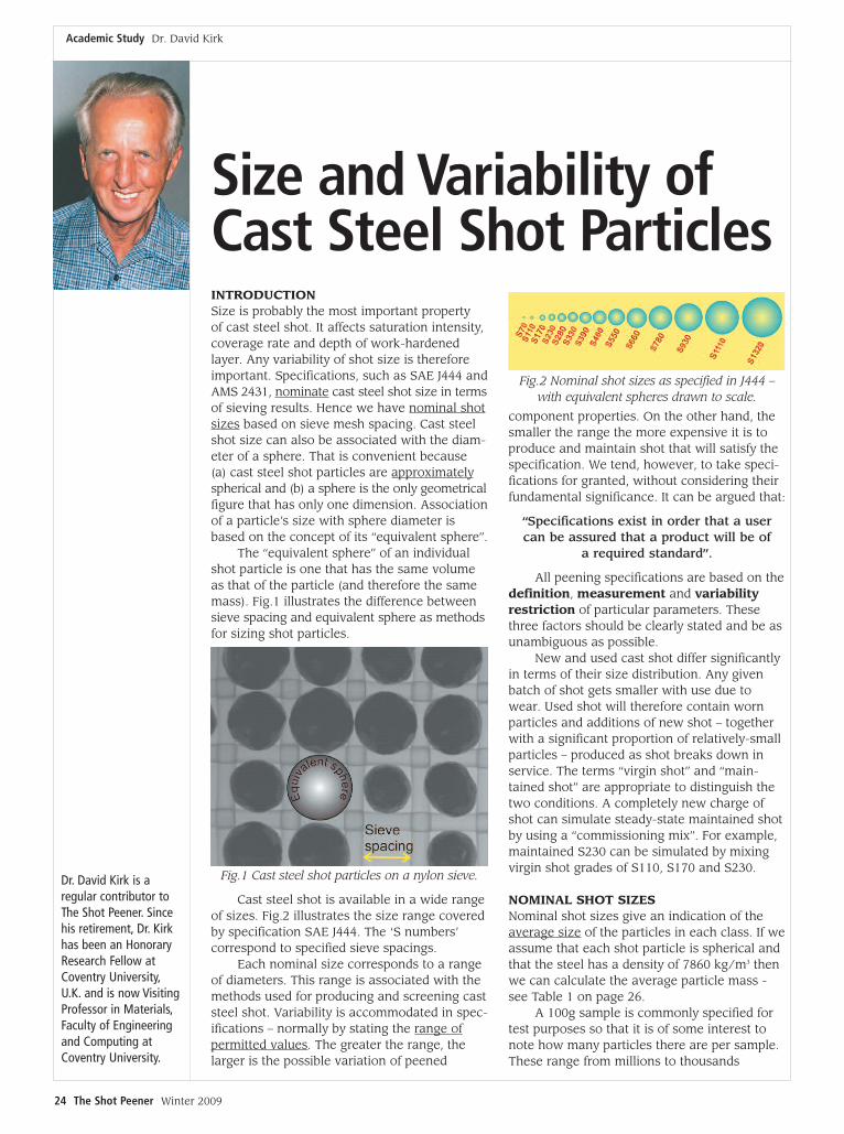
24 The Shot Peener Winter 2009

Size and Variability ofCast Steel Shot Particles

Academic Study Dr. David Kirk

INTRODUCTIONSize is probably the most important propertyof cast steel shot. It affects saturation intensity,coverage rate and depth of work-hardenedlayer. Any variability of shot size is thereforeimportant. Specifications, such as SAE J444 andAMS 2431, nominate cast steel shot size in termsof sieving results. Hence we have nominal shotsizes based on sieve mesh spacing. Cast steelshot size can also be associated with the diam-eter of a sphere. That is convenient because(a) cast steel shot particles are approximatelyspherical and (b) a sphere is the only geometricalfigure that has only one dimension. Associationof a particle’s size with sphere diameter isbased on the concept of its “equivalent sphere”.

The “equivalent sphere” of an individualshot particle is one that has the same volumeas that of the particle (and therefore the samemass). Fig.1 illustrates the difference betweensieve spacing and equivalent sphere as methodsfor sizing shot particles.

Fig.1 Cast steel shot particles on a nylon sieve.

Cast steel shot is available in a wide rangeof sizes. Fig.2 illustrates the size range coveredby specification SAE J444. The ‘S numbers’ correspond to specified sieve spacings.

Each nominal size corresponds to a rangeof diameters. This range is associated with themethods used for producing and screening caststeel shot. Variability is accommodated in spec-ifications – normally by stating the range ofpermitted values. The greater the range, the larger is the possible variation of peened

component properties. On the other hand, thesmaller the range the more expensive it is toproduce and maintain shot that will satisfy thespecification. We tend, however, to take speci-fications for granted, without considering theirfundamental significance. It can be argued that:

“Specifications exist in order that a user can be assured that a product will be of

a required standard”.

All peening specifications are based on thedefinition, measurement and variabilityrestriction of particular parameters. Thesethree factors should be clearly stated and be asunambiguous as possible.

New and used cast shot differ significantlyin terms of their size distribution. Any givenbatch of shot gets smaller with use due towear. Used shot will therefore contain wornparticles and additions of new shot – togetherwith a significant proportion of relatively-smallparticles – produced as shot breaks down inservice. The terms “virgin shot” and “main-tained shot” are appropriate to distinguish thetwo conditions. A completely new charge ofshot can simulate steady-state maintained shotby using a “commissioning mix”. For example,maintained S230 can be simulated by mixingvirgin shot grades of S110, S170 and S230.

NOMINAL SHOT SIZESNominal shot sizes give an indication of theaverage size of the particles in each class. If weassume that each shot particle is spherical andthat the steel has a density of 7860 kg/m3 thenwe can calculate the average particle mass -see Table 1 on page 26.

A 100g sample is commonly specified fortest purposes so that it is of some interest tonote how many particles there are per sample.These range from millions to thousands

Dr. David Kirk is aregular contributor toThe Shot Peener. Sincehis retirement, Dr. Kirkhas been an HonoraryResearch Fellow atCoventry University,U.K. and is now VisitingProfessor in Materials,Faculty of Engineeringand Computing atCoventry University.

Fig.2 Nominal shot sizes as specified in J444 –with equivalent spheres drawn to scale.

26 The Shot Peener Winter 2009

depending on shot size. 100kg of S110 circulating in apeening unit will consist of about a billion shot particles!

PRODUCTION VARIABILITYNominal shot size is a fixed quantity whereas actual samplescontain a range of sizes. This range depends on productionvariability and associated screening procedures.

Cast steel shot is produced directly from the liquid state.The method employed is the prime cause of size variability.Liquid steel is poured from a ladle into high-pressure jetsof water. The water jets break up the steel stream into tinydroplets that solidify to become shot particles. Dropletsstrive to reduce surface energy by minimizing the surfacearea-to-volume ratio. A spherical shape has the smallestsurface area-to-volume ratio. Hence, as-cast shot particlesapproximate to spheres. Fig.3 illustrates possible variationsof shot particle sizes produced by one ladleful of steel.These are close to what are called “normal distributions”.The distribution has a mean that can be controlled, to alimited extent, by factors such as water jet pressure andgeometry. Variation about the mean can be quantified byits variance value (square of standard deviation).

The mass/size variations shown in fig.3 include only asmall proportion of the most commercially-important shotsizes (such as S110, S170 and S230). A grit fraction couldgo directly to crushing - because the water-quenched stateis very brittle. Normally, however, the whole output is classified, then austenized and quenched before rough

screening to separate potential grit and shot fractions. Theshot fraction is tempered and fine screened in order toyield different specification sizes of virgin shot.

Fine screening divides the shot fraction into sub-frac-tions – each of which will satisfy a corresponding standardspecification. Precise details of fine screening are kept confidential by manufacturers. Fig.4 represents a possiblescreening routine designed to satisfy J444. Consider, forexample, the S70 fraction - separated by having it passthrough a 0·355mm sieve but not passing through a0·125mm sieve. This would satisfy the J444 requirement of"All pass 0·425mm, 10% max on 0·355mm, 80% min on0·180mm and 90% min on 0·125mm". The S110, S170 andS270 fractions shown would also satisfy the correspondingJ444 requirements.

Fig.4 Possible screening system for cast steel shot.

Each nominal size of virgin shot will contain a rangeof sizes. For S70 produced using the procedure indicated infig.3 the size range would be from 0·125mm to 0·355mm indiameter. The mass of a shot particle is its volume multi-plied by the steel’s density. Volume of a sphere is ππd3/6(d being diameter). Hence the range of mass is the cube ofthe range of diameters. For the previous S70 example, therange of mass would be (0·355/0·125)3 or 22·9 to 1! Massranges would be only 2·8 to 1 for S110, 2·9 to 1 for S170and 1·7 to 1 for S230 respectively. If the shot manufacturerneeded to produce smaller shot than S70 then the lowerend of the S70 grade range could be reduced to 0·180mmwhich would still satisfy J444. The mass range would thenbe reduced to 7·7 to 1 for the finer-screened S70.

SIZE SPECIFICATION TESTINGA typical size specification test involves taking a 100gsample of a given batch, sieving it with a set of standardsieves and weighing the sieved fractions. This type of testinvolves several sources of variability. One is the sampleitself – which has to be selected from a large batch of shot.Various techniques, such ‘splitter boxing’, have beendeveloped to ensure that the sample is reasonably repre-sentative. Another source of variability is that if we subjectthe same 100g sample to repeat testing then the weightswill vary – albeit slightly. A third, more significant, sourceof variability is that of the sieves themselves. The individualopenings in a given brand-new sieve vary in size – evenwith the highest quality of sieves. Wear in use exacerbatesthe variation in opening size - as well as causing the aver-age opening size to drift to larger values. One noteworthy

Academic Study Dr. David Kirk

Table 1. Nominal Shot Sizes derived from J444 using‘Equivalent Sphere’ principle

Fig.3. Type of size variability for as-cast steel shot.

28 The Shot Peener Winter 2009

feature is the very large numbers of particles that are present in a 100g sample – for example, about a million for100g of S110.

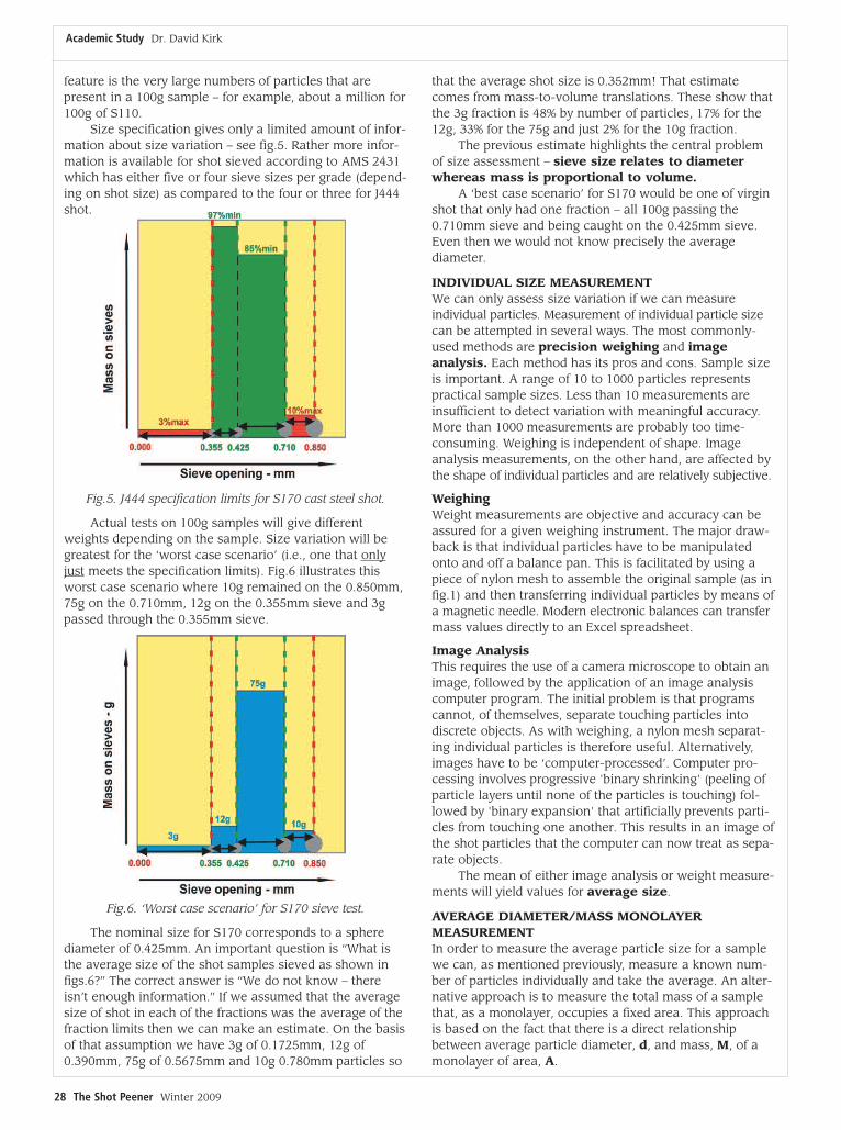
Size specification gives only a limited amount of infor-mation about size variation – see fig.5. Rather more infor-mation is available for shot sieved according to AMS 2431which has either five or four sieve sizes per grade (depend-ing on shot size) as compared to the four or three for J444shot.

Fig.5. J444 specification limits for S170 cast steel shot.

Actual tests on 100g samples will give differentweights depending on the sample. Size variation will begreatest for the ‘worst case scenario’ (i.e., one that onlyjust meets the specification limits). Fig.6 illustrates thisworst case scenario where 10g remained on the 0.850mm,75g on the 0.710mm, 12g on the 0.355mm sieve and 3gpassed through the 0.355mm sieve.

Fig.6. ‘Worst case scenario’ for S170 sieve test.

The nominal size for S170 corresponds to a spherediameter of 0.425mm. An important question is “What isthe average size of the shot samples sieved as shown infigs.6?” The correct answer is “We do not know – thereisn’t enough information.” If we assumed that the averagesize of shot in each of the fractions was the average of thefraction limits then we can make an estimate. On the basisof that assumption we have 3g of 0.1725mm, 12g of0.390mm, 75g of 0.5675mm and 10g 0.780mm particles so

that the average shot size is 0.352mm! That estimatecomes from mass-to-volume translations. These show thatthe 3g fraction is 48% by number of particles, 17% for the12g, 33% for the 75g and just 2% for the 10g fraction.

The previous estimate highlights the central problemof size assessment – sieve size relates to diameterwhereas mass is proportional to volume.

A ‘best case scenario’ for S170 would be one of virginshot that only had one fraction – all 100g passing the0.710mm sieve and being caught on the 0.425mm sieve.Even then we would not know precisely the average diameter.

INDIVIDUAL SIZE MEASUREMENTWe can only assess size variation if we can measure individual particles. Measurement of individual particle sizecan be attempted in several ways. The most commonly-used methods are precision weighing and image analysis. Each method has its pros and cons. Sample sizeis important. A range of 10 to 1000 particles representspractical sample sizes. Less than 10 measurements areinsufficient to detect variation with meaningful accuracy.More than 1000 measurements are probably too time-consuming. Weighing is independent of shape. Imageanalysis measurements, on the other hand, are affected bythe shape of individual particles and are relatively subjective.

WeighingWeight measurements are objective and accuracy can beassured for a given weighing instrument. The major draw-back is that individual particles have to be manipulatedonto and off a balance pan. This is facilitated by using apiece of nylon mesh to assemble the original sample (as infig.1) and then transferring individual particles by means ofa magnetic needle. Modern electronic balances can transfermass values directly to an Excel spreadsheet.

Image AnalysisThis requires the use of a camera microscope to obtain animage, followed by the application of an image analysiscomputer program. The initial problem is that programscannot, of themselves, separate touching particles into discrete objects. As with weighing, a nylon mesh separat-ing individual particles is therefore useful. Alternatively,images have to be ‘computer-processed’. Computer pro-cessing involves progressive 'binary shrinking' (peeling ofparticle layers until none of the particles is touching) fol-lowed by 'binary expansion' that artificially prevents parti-cles from touching one another. This results in an image ofthe shot particles that the computer can now treat as sepa-rate objects.

The mean of either image analysis or weight measure-ments will yield values for average size.

AVERAGE DIAMETER/MASS MONOLAYER MEASUREMENTIn order to measure the average particle size for a samplewe can, as mentioned previously, measure a known num-ber of particles individually and take the average. An alter-native approach is to measure the total mass of a samplethat, as a monolayer, occupies a fixed area. This approachis based on the fact that there is a direct relationshipbetween average particle diameter, d, and mass, M, of amonolayer of area, A.

Academic Study Dr. David Kirk

30 The Shot Peener Winter 2009

For ‘square-packed’ spheres the number of particles,n, occupying an area, A, is given by n = A/d2. The mass,m, of one particle is given by ρρ*ππ*d3/6. The mass, M, ofthe n particles occupying the area, A, is therefore given by: M = A/d2*ρρ*ππ*d3/6 which simplifies to equation (1).

d = 6M/A*ρρ*ππ (1)where ρρ = density.

Fig.7 serves to illustrate equation (1), using identical‘square-packed’ spherical particles.

The principle embodied inequation (1) can be appliedby spreading a shot sampleover a fixed area. The samplesize will normally contain avery large number of parti-cles. 10g of S110, for exam-ple, would contain more than100,000 particles. Imagine, asa hypothetical example, asample of S110 shot that hasan average diameter that isexactly 0·0110" and, whenspread over a fixed area, hasa mass of precisely 10·00g. A 1% increase in samplediameter, other things beingequal, would raise the massto 10·10g.

Such a mass change isreadily detected using thescales required for standardsieve tests.

Shot particles simplypoured into a circular dish do not readily form a truemonolayer. Fig.8 shows a number of ‘second layer’ particlestogether with ‘vacant particle sites’ (black dots versus whiteareas). Layers equivalent to monolayers can be producedin a few seconds by equating the numbers of ‘second layer’and ‘vacant particle sites’. Reproducibility of layer mass isthen excellent – better than 0·1g for samples of about 10g.True monolayer production requires more sophisticatedtechniques than simple pouring. Gaging approach to truemonolayer achievement is facilitated by projecting a magnified image from a digital camera onto a computer/TV screen.

Fig.8 SLR camera image of S330 shot sample viewed through a light box.

SIZE VARIATION ANALYSISThe two most useful procedures for representing size variation are:

HISTOGRAMS and BOXPLOTS.

HistogramsHistograms are based on dividing measurements into ‘bins’– each bin containing all of the measurements that liewithin a defined range. Figs.9 and 10 are histograms of'number of particles in a given bin for 69 weighed particlesof S780 shot. The mass measurements plotted in fig.9 wereconverted into diameters of 'equivalent spheres' for plottingas fig.10.

There are pros and cons attached to the use of histograms – some of which are indicated in figs. 9 and 10.Different types of distribution result from plotting differentparameters. Mass variation appears to be skewed towardslower values whereas diameter variation appears to be bi-modal. The test sample originated from shot that hadbeen segregated (by sieving) according to diameter. It ispossible that the sample is a mixture of two sievings –each being normally-distributed about a different mean.Bin size, parameter and range strongly affect implied typesof distribution.

Histograms do not yield quantitative parameters ofdistribution. Their strongest feature is that they present afamiliar type of visual image. Data acquired for histogramanalysis can be used to determine complementary parameters such as range, mean and standard deviation.

Fig.9 Histogram of S780 weighed particles – mass versus number per bin.

Fig.10 Histogram of S780 weighed particles – diameter versus number per bin.

Academic Study Dr. David Kirk

Fig.7. Effect of sphere diameter on number of particles per unit area.

32 The Shot Peener Winter 2009

BoxplotsBoxplots depict, graphically, a summary of five parametersobtained from a set of measurements. The five parametersare: Minimum value, Maximum value, Lower quartile(Q1), Median and Upper quartile (Q3). “Median” is themiddle value of a set of measurements – hence half of themeasurements are larger than that of the median and halfare smaller. “Quartile” is a quarter of the total number ofmeasurements. It follows that the ‘box’ contains half of the measurements whilst a quarter are ‘above’ and theremaining quarter are below the box. Excel uses its ownsystem for determining quartiles – together with minimum,maximum and median values.

Fig.11 shows a set of three Boxplots derived fromhypothetical data using Excel. This illustrates how we canreadily compare, quantitatively, the most important sizeparameters of shot in terms of difference.

Unlike histograms, Boxplots are completely objectivein the sense that they are independent of plotting variables(such as bin size, number of bins etc.). That feature is particularly useful when it comes to possible specificationconsiderations.

Interpretation of Boxplots gets easier with practice.This particularly applies to the very useful ‘position ofmedian within the box’.

Fig.11. Boxplot comparison of three hypothetical samples.

DISCUSSION AND CONCLUSIONSThis article has considered only cast steel shot – ratherthan the full range of types and materials that are commer-cially available for peening. That is in order to contain thearticle within a reasonable size whilst avoiding superficiality.The principles described using J444 can easily be extendedto AMS 2431 shot specification.

The origin of variability lies with the casting process.Subsequent sieving operations are used to produce speci-fied size grades. Size testing based on standard sieve testson 100g samples yields restricted amounts of informationin terms of size distribution and none on actual averagesize. Image analysis is now readily available and offers away of obtaining much more detailed information. Care

Academic Study Dr. David Kirk

must be taken to ensure that the image analysis procedureused on samples gives repeatable, consistent, results.

100g samples used for sieve testing are much largerthan those used for image analysis. Even greater caremust therefore be taken to ensure that image analysissamples are representative.

Analysis of size variation based on either imageanalysis or weight measurements can be carried out usingeither histograms or Boxplots. It is suggested that Boxplotsare much more suitable than histograms as a basis forboth specifications and quality control.

It has been proposed in this article that average sizemeasurements can be made by weighing monolayers ofknown area. Preliminary results are very encouraging andtechniques are being developed to facilitate monolayerproduction. l

Almen Saturation Curve Solver Program

Get the program developed by Dr. David Kirk

Request the FREE program at:

www.shotpeener.com/learning/solver.php