Credit Rationing in Markets with Imperfect InformationBy Joseph E. Stiglitz and Andrew Weiss

Presented by Lara Converse, Elyas Fermand, Aditya Rachmanto, and Annie TaoJanuary 24, 2012

Introduction

Credit markets are characterized by “credit rationing,” a situation in which there appears to be

excess demand for funds. While certain policies (i.e. usuary laws) or interest rate “stickiness”

may be the cause of some cases of excess demand in credit markets, Stiglitz and Weiss argue that

credit rationing may occur as an equilibrium (hence, “equilibrium rationing”), due to imperfect

information faced by banks.

There are two main effects:

i. Adverse selection effect—banks are forced to rely on “screening devices” (like interest

rates, for example) to determine which of their borrowers are most likely to repay their

loan. Riskier individuals are willing to pay higher interest rates because their probability

of default is relatively high. As firms raise interest rates, they are likely to attract only

the riskiest borrowers.

ii. Incentive effect—Borrowers change their behavior in response to an interest rate

changes. Higher interest rates promote a choice of riskier projects.

1

Facing these effects, there is a “bank

optimal” interest rate (r*) at which the

bank’s expected return is maximized, as

seen in Figure 1.

While at r* there may be an excess demand for funds, this is an equilibrium interest rate.

Even prospective borrowers who offered to pay higher interest rates would be declined due to the

bank’s expectation of a loan to them to be risky. A Walrasian market equilibrium will not be

attained. Importantly, people who are “observationally equivalent” to those who receive loans

are denied credit.

Formally, credit-rationing is defined as cases in which:

“a) Among loan applicants who appear to be identical some receive a loan and others do not, and the rejected applicants would not receive a loan even if they offered to pay a higher rate; OR

b) There are identifiable groups of individuals in the population who, with a given supply of credit, are unable to obtain loans at any interest rate, even though with a larger supply of credit, they would.”

Key Assumptions

There are many banks and borrowing firms. Both banks and firms are driven by profit-

maximizing motives. Banks may choose their interest rate and the required collateral.

Probability distributions of project success vary by firm, but banks cannot identify safe projects

from risky projects through any defining characteristics of the firm. Firms and banks are risk

neutral and projects are not divisible. The supply of funds is independent of the interest rate

charged. All loans are of equal size.

Significance of the Paper

This paper offers the first theoretical explanation of credit rationing, adding to a literature

of other explanations of borrowing behavior. The theory developed in this paper can be

extended to other instances of the principal-agent problem, including relationships between

landlords and tenants or between employees and employers.

2

Key Notation

r* Bank-optimal interest rater Interest raterm Walrasian equilibrium interest rate

θ Risk level of a projectR Returns to a projectF(R,θ) Distribution of returns (cumulative density function)f(R, θ) Density function of returns (probability density function)B Dollar amount of the loan (often normalized to equal 1)C Dollar amount of collateralπ Firm profit/returnρ Returns earned by the bankρ Mean returns earned by the bankZ Excess demand for fundsλ Fraction of the population that is infinitely risk averseG(.) Distribution of characteristics of alternative projects (cumulative density function)g(.) Density function of characteristics of alternative projects (probability density

function)W0 Initial WealthL Dollar amount of loan in first periodM Dollar amount of loan in second period

I. Interest Rate as a Screening Device

Borrowing firms wish to maximize their profits and banks wish to maximize their returns.

Note that the net return to the borrower is given by:

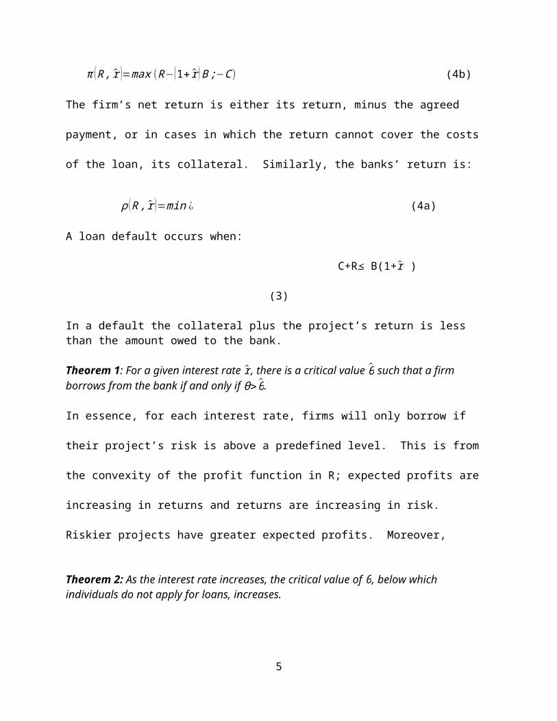
π (R ,r )=max (R−(1+r )B ;−C ) (4b)

The firm’s net return is either its return, minus the agreed payment, or in cases in which the

return cannot cover the costs of the loan, its collateral. Similarly, the banks’ return is:

ρ (R , r )=min ¿ (4a)

A loan default occurs when:

C+R≤ B(1+r ) (3)

In a default the collateral plus the project’s return is less than the amount owed to the bank.

3

Theorem 1:Foragiveninterestrater,thereisacriticalvalueθsuchthatafirmborrowsfromthebankifandonlyifθ>θ.

In essence, for each interest rate, firms will only borrow if their project’s risk is above a

predefined level. This is from the convexity of the profit function in R; expected profits are

increasing in returns and returns are increasing in risk. Riskier projects have greater expected

profits. Moreover,

Theorem 2: Astheinterestrateincreases,thecriticalvalueofθ,belowwhichindividualsdonotapplyforloans,increases.

This is evident from the positive sign of the derivative of the expected profit function (5) given

in (6).

(6)

At higher interest rates, firms will only apply for loans for riskier projects as these projects yield

higher expected profits.

Figure 2 illustrates these theorems:

In (2a), the horizontal section represents such low levels of returns that the collateral is greater

than the net return from the project, so the firm pays the collateral. When (1+ r ¿B >R> (1+

r ¿B−C , the firm faces negative net returns, but does not pay its collateral. Net returns are

4

positive when R> (1+ r ¿B. In 2(b), the bank earns (1+ r ¿B>ρ≥C when R<(1+ r ¿B−C . For

higher returns, the bank earns (1+ r ¿B.

Theorem 3:Theexpectedreturnonaloantoabankisadecreasingfunctionoftheriskinessoftheloan.

Risky loans yield lower returns to the bank, as is evident from the concavity of the ρ(R, r) in R

in Figure 2B.

Theorem 4:Ifthereareadiscretenumberofpotentialborrowers(ortypesofborrowers)eachwithadifferentθ,ρ(r ¿willnotbeamonotonicfunctionofr,sinceaseachsuccessivegroupdropsoutofthemarket,thereisadiscretefallinρ(whereρ(r ¿isthemeanreturntothebankfromasetofapplicantsattheinterestrater.

Theorem 5:Wheneverρ(r ¿hasaninteriormode,thereexistsupplyfunctionsoffundssuchthatcompetitiveequilibriumentailscreditrationing.

Theorem 5 explains credit rationing, as it indicates that, as seen in Figure 3 above, when ρ(r ¿

takes a non-monotonic form, banks may ration credit in order to set r at the non-Walrasian

equilibrium rate for which the safe loans remain in the market and ρ(r ¿ is maximized.

5

This theorem is illustrated in Figure 3. For low levels of r,

rcan be raised slightly andboth firms with risky projects

and firms with safe projects will still apply for loans, which

will increase ρ. However, as r rises above a certain level

(r1), the safe borrowers will be no longer be willing to

borrow funds, so only risky loans will be made, thus the ρ

will decline. This is an adverse selection effect.

The Walrasian equilibrium point is at rm, but banks will supply credit at their optimal rate, r*. Z

represents the excess demand at this interest rate. In the lower left quadrant, note that Ls need

not be increasing inρ.

Note also the comparative statics implied by Figure 4:

Corollary 1:Asthesupplyoffundsincreases,theexcessdemandforfundsdecreases,buttheinterestratechargedremainsunchanged,solongasthereisanycreditrationing.

With a sufficient extension of funds, excess funds (Z) will equal zero. This is evident through an

upward shift in Ls in the upper right quadrant. If supply continues to increase, rm will fall.

Theorem 6:Iftheρ(r ¿functionhasseveralmodes,marketequilibriumcouldeitherbecharacterizedbyasingleinterestrateatorbelowthemarket-clearinglevel,orbytwointerestrates,withanexcessdemandforcreditatthelowerone.

According to Theorem 6, there are two potential cases if the ρ(r ¿ function has several modes,

depending on the relationship between r and rm.

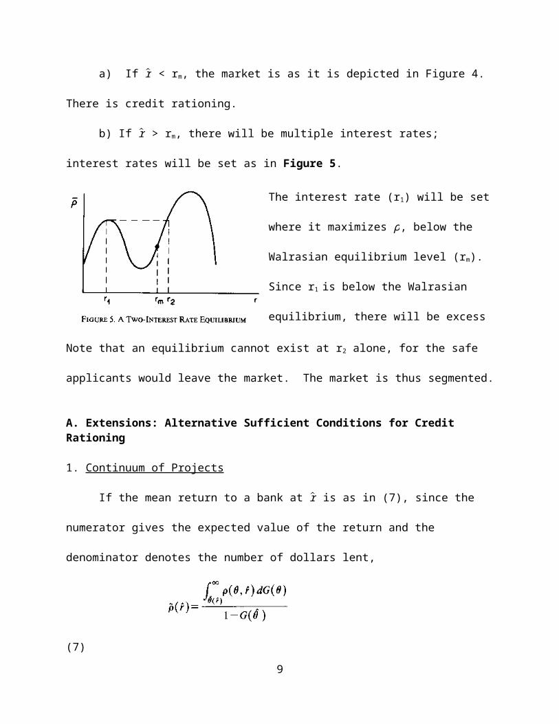
a) If r < rm, the market is as it is depicted in Figure 4. There is credit rationing.

b) If r > rm, there will be multiple interest rates; interest rates will be set as in Figure 5.

6

Figure 4 helps to illustrate Theorem 5.

Note that the curve relating interest rates

and ρ in the bottom right quadrant is non-

monotonic, and ρ is maximized at r*. In

the upper right quadrant, demand for funds

declines with the interest rate.

Note that an equilibrium cannot exist at r2 alone, for the safe applicants would leave the market.

The market is thus segmented.

A. Extensions: Alternative Sufficient Conditions for Credit Rationing

1. Continuum of Projects

If the mean return to a bank at r is as in (7), since the numerator gives the expected value

of the return and the denominator denotes the number of dollars lent,

(7)

and (7) is differentiated with respect to r,

(8)

it is clear that ρ decreases with r (dρ /dr <0) if the first term is larger in absolute value than the

second term. Negativity of dρ /dr would indicate non-monotonicity of the loan supply function,

providing the conditions for credit rationing (Theorem 5). The first term is larger than the

second term if ¿ -ρ) is large, meaning the return on the safest loans is much larger than the mean

7

The interest rate (r1) will be set where it maximizes ρ

, below the Walrasian equilibrium level (rm). Since r1

is below the Walrasian equilibrium, there will be

excess demand. A second interest rate (r2) such that

ρ ¿r1)=ρ(r2) will be chosen. All funds available at ρ ¿

r1) will be loaned with r1 and r2.

returns, or if g ¿¿is large, meaning an increase in the interest rate greatly increases the riskiness

of the prospective loaners. Therefore, if these two conditions hold, credit-rationing would be

observed.

2. Two Outcome Projects

Assume there are projects that either succeed (return=S<R<K) or fail (return=D). Let

B=1, C=0, and each project have same expected return. Let p(R)=probability of success, J= r+1,

and assume that each defaulted dollar of loan costs the bank X dollars. The expected return per

dollar is given by:

(10)

since the coefficient essentially represents the number of dollars loaned, while the first term

inside the brackets represents the bank’s returns from successful projects. The second bracketed

term is the bank’s losses from failed profits.

From mathematics referenced in the mathematical appendix, δρ (J )/δJ<0 under three

conditions:

8

If any of these three cases hold, ρ will display

non-monotonicity, and there will be credit-

rationing.

3. Differences in Attitudes Towards Risk

Risk averse loan applicants will favor safe projects, but safe projects will not be chosen if

interest rates are high. Therefore, differences in risk aversion can influence the bank-optimal

interest rate (r*) and lead to credit rationing. Let λ represents the fraction of applicants that are

infinitely risk averse and have G(R) as their distribution of returns function. If another group of

risk neutral applicants invests in projects that have a probability pof earning return R*>K and

probability (1-p) of zero return, the bank’s expected return is given by:

(11)

since the numerator gives the returns from the successful projects (first term: risk averse

applicants; second term: risk neutral applicants), while the denominator provides the total

number of loans.

Differentiate lnρ with respect to ln(1+r) to get:

(12)

For an interior optimal interest rate, limR->K∂ ρ /∂ r <0. Written as,

λ /(1− λ)

it is clear that if p is small (risky project), the expression is more likely to hold, so an interior

optimal interest rate is more likely. Additionally, if a larger fraction of applicants are risk averse

(large ¿(1−λ)¿ , an interior optimal interest rate is likely. It is evident that the strong risk

aversion of some borrowers can restrict lending through credit rationing, as banks choose their

9

optimal r* at levels in which even the most risk averse people will choose to borrow.

Theoretically, this situation could interfere with technological progress because “risky”

entrepreneurs might lack access to the credit they need for innovation.

II. Interest Rate as an Incentive Mechanism

Borrowing firms are interested primarily in their investment’s returns, but banks are

interested in the firm’s avoidance of bankruptcy. Noting these differential incentives, banks may

use the interest rate in order to influence borrowers’ behavior.

Theorem 7:If,atagivennominalinterestrater,arisk-neutralfirmisindifferentbetweentwoprojects,anincreaseintheinterestrateresultsinthefirmpreferringtheprojectwiththehighestprobabilityofbankruptcy.

Essentially, all else equal, as interest rates rise, firms prefer riskier projects. This is evident from

the derivative of the borrower’s expected returns function:

(14)

Since (1-Fi((1+r)B-C))>0 because F is a distribution function, dπ/dr <0. Since expected returns

fall as interest rates rise, a profit-maximizing firm will increase the riskiness of its chosen project

in the face of higher interest rates (see Theorem 2). Combining Theorem 7 with Theorem 3, as

the interest rate rises, firms choose riskier projects, and the bank’s expected return decreases.

10

Consider Figure 6:

Since the firm is indifferent between projects A and B at r, their expected returns are equal:

(15)

Solving (15) for r gives:

(16)

which gives r* as shown in Figure 6. When interest rates are below r*, the firm will do project

B (the safe project) because the low interest rate will generally give the safer project a higher

expected return. Since Ra/B is the maximum return to project A, if r is such that r*<r<(( Ra/B)-

1), the firm will choose project B. The bank may practice credit-rationing in order to influence

project choice of the borrowers in a way that maximizes their returns. In particular, r* will

provide the maximum expected return if and only if:

Simplification of this term indicates that r* is optimal if:

(a) pbRb>paRa,

(b) (1+r*)>0, and

(c) ρ is not monotonic in r.

11

Consider two projects. If successful, one provides

returns Ra (prob=pa), the other provides Rb

(prob=pb). Let Ra>Rb and C=0.

II. The Theory of Collateral and Limited Liability

Banks will not increase collateral requirements because doing so may result in adverse

selection. Two examples:

(a) If smaller projects are riskier, for instance, increasing the required collateral (as a proportion of the equity) will result in banks funding riskier projects over larger, safer ones.

(b) Assuming wealthy borrowers are likely less risk averse (perhaps their wealth is due to past success on risky projects), they are more likely than less wealthy, more risk averse individuals to have the funds available to meet high collateral requirements.

Assumptions: All borrowers are risk averse and have identical utility functions, U(W), with

U’(W)>0, U’’(W)<0, but different amounts of original wealth (W0). Each of the borrower’s

considered projects have a success rate of p(R), with R as the return. B=1. If the project fails, the

return is zero. There is an option for a safe project with return ρ*. The bank is unable to

determine the borrowers’ wealth or project choice.

Theorem 9:Thecontract{C,r}actsasascreeningmechanism:thereexisttwocriticalvaluesof

W0,W 0andW⏞0,suchthatifthereisdecreasingabsoluteriskaversionallindividualswithwealth

W 0<W0<W⏞0applyforloans.

This theorem states that under decreasing absolute risk aversion, there is a defined range of

initial wealth levels under which individuals will apply for loans.

This can be seen through simple derivations. The expected utility of a self-financed project

(investment=$1) is given by V (W0):

(17)

12

The individual will choose either to self-finance or complete the safe project (providing

U(W0p*)) by maximizing utility:

(18)

Differentiating U(W0p*) and V (W0) with respect to W0:

Under decreasing absolute risk aversion,

Therefore, there is a defined level of wealth, W⏞0, such that, if initial wealth W0 > W⏞0, the

individual will self-finance the project. This inequality corresponds to the slope of the lines in

Figure 7.

If the person borrows, his expected utility is given by:

(21)

But he will only borrow if his utility from borrowing is at least as great as his utility if he doesn’t

borrow:

(22)

Noting that:

13

(19)

(20)

(23)

(20) and (23) imply:

at W0

Therefore, individuals with initial wealth W0, for which W 0 < W0 < W⏞0,will apply for loans, and

for W0 < W⏞0, only the wealthiest will borrow.

This finding is displayed in Figure 7 below.

Collateral has opposing effects on a bank’s return:

Theorem 11: Collateralincreasesthebank’sreturnfromanygivenborrower:dp/dC>0

However, adverse selection effects from collateral may reduce the bank’s return, as:

Theorem 12: Thereisanadverseselectioneffectfromincreasingthecollateralrequirement,i.e.,boththeaverageandthemarginalborrowsisriskier,dW 0/dC > 0.

Simply, this theorem states that increased collateral requirements attract wealthier and riskier

borrowers. This can be shown through differentiation of (21) to get:

14

For W0 below W 0, all individuals will choose to

self-finance the safe projects because it yields

the highest expected utility. Between W 0 and W⏞

0, all individuals will borrow to finance the risky

projects. As wealth exceeds W 0 but is less than

W 0, individuals will choose to borrow. Past W 0,

the individual will self-finance.

Overall, as displayed in Figure 8, the effect of increasing collateral requirements may be

positive or negative for the bank’s return. The bank’s return will rise as collateral requirements

rise, but only up to a certain point. After this threshold of collateral requirement, the safe, low

wealth applicants will no longer seek loans, which would cause a fall in the bank’s return.

A. Adverse Incentive Effects in a Multiperiod Model

In a multi-period model in which the bank can make multiple loans to the same borrower,

the borrower may face incentives to act in ways to secure future loans from the bank. Assume in

the first period, success (θ) earns a return to the firm of R1 and occurs with probability p1. The

first period project is funded with loan L. If the project is unsuccessful, the project will have

zero return, or else more funds (M) are needed in the second period. The second-period funding

will be loaned at r2. The expected return to the firm is given by:

with

The first term represents the net return on the first period’s investment, repaid in period 2, and

the second term represents the net return to both periods’ investments, if there was a loan in the

second period. Since the bank cannot fully control the expected value of its loans because the

15

firm chooses the riskiness of the project, the firm may respond to a reduction in L by increasing

M. As a result, it is possible that a reduction in L may reduce the bank’s returns.

III. Observationally Distinguishable Borrowers

If borrowers are no longer assumed to be identical, this theory offers new insights.

Assume there are ngroups that can be observationally distinguished. Let each group have a

bank optimal interest rate r*. If ρi(r i) represents the gross return to a bank from type i’s optimal

interest rate, the returns can be ordered such that maxρi(r i)>maxρj(r j).

Theorem 13:Fori>j,typejborrowerswillonlyreceiveloansifcreditisnotrationedtotypeiborrowers.

This can be understood intuitively. From the ordering assumptions, loans to j yield lower returns

to the bank than loans to i. Therefore, the bank will maximize profits by choosing to loan to type

i instead of type j. Type jwill only receive loans if banks have not rationed credit to only supply

type iborrowers.

Figure 9 illustrates this point:

borrowers, the interest rate will fall to yield a return equal to the cost of funds. Some type 2

borrowers will receive funds at r2*. Type 1 borrowers are completely excluded from the market.

They will not receive funds because the bank’s return from the interest rate they would be

16

As seen in the figure, depending on cost of funds (ρ),

some types of borrowers will be “redlined,” or unable

to obtain credit. For instance, consider ρ*: type 3

borrowers will be provided loans at ~r3 since the

bank’s optimal interest rate for type 3 yields returns

greater than ρ*, but through competition for these

charged is less than the cost of funds ρ** < ρ*. Type 1 borrowers have been redlined (with cost

of funds at ρ*, there is no interest rate for which they can get loans). These borrowers, may:

(a) Have riskier investments, although the total expected return (return to bank and firm)

may be higher than Type 3’s investments

(b) Their investments may be harder to “filter” (harder to identify riskiest loans)

(c) Have access to a wider range of types of projects (including both safe and risky

projects) but choose to invest in risky projects for the higher expected returns

It is important to note that with redlining, a market equilibrium may not distribute credit to the

investments with the highest expected return. Higher risk yields higher expected returns, yet

investments in risky projects may not be funded.

IV. Debt vs. Equity Finance, Another View of the Principal Agent Problem

Other Applications

This paper can be applied to other contexts of the principal-agent problem (i.e.: landlord

and tenant). In considering the rental structure for sharecroppers, for instance, fixed fee

contracts may discourage risk averse tenants but not risk neutral tenants. Adverse incentives may

still play a role, as tenants still control their probability of bankruptcy.

Criticisms

Restricting analysis to a single period does not permit “rewards” for known “safe”

borrowers through lower interest rates. Borrowers would then be encouraged to invest in safe

projects.

17

V. Conclusions

Among observationally equivalent borrowers under credit rationing, some borrowers are

denied credit, even if they have a willingness to pay a higher interest rate or offer more

collateral. Banks set an interest rate at a level low enough so that safe borrowers will remain in

the market for funds, as it is at this level that bank profits are maximized. In general, the credit

rationed supply of funds will be less than the Walrasian equilibrium supply of funds.

Excess supply of credit is also possible due to imperfect information. As in the following

situation, for example: Bank A knows which of their borrowers are most profitable, but

competing banks do not. Competing banks then offer the customers of Bank A lower interest

rates. Bank A will lower its interest rate to keep these safe borrowers. Risky borrowers will

move to the other banks. At equilibrium, there will be an excess supply of credit, for firms will

not lower their interest rates.

Acknowledgments

Thanks to Huichun Sun, Salama Freed, and the group who presented this paper in Spring 2011

for enhancing our understanding.

18

APPENDIX I: DERIVATIONS

I. Interest Rate as a Screening Device

Theorem 2: Astheinterestrateincreases,thecriticalvalueofθ,belowwhichindividualsdonotapplyforloans,increases.

Proof:The value of θ for which expected profits are zero satisfies:

(5)Total differentiating (5) with respect to r and θ, we get:

, since , , and .

A. Alternative Sufficient Conditions for Credit Rationing

1. Continuum of Projects

Let G(θ) be the distribution of projects by riskiness θ, and ρ(θ,r) be the expected return to the bank of a loan of risk θ and interest rate r. For a mean return to the bank , we know from

Theorem 5 that for some value of r is a sufficient condition for credit rationing. The mean return to the bank which lends at the interest rate r is simply:

(7)

Let , and differentiating (7) with respect to r, then we have:

19

From (4b), we know that the value of θ which expected profits are zero satisfies:

Differentiating with respect to r, we get:

Substituting this, we get:

depending on the relative sizes of the two terms

2. Two Outcome Projects

From the bank’s perspective, the projects have two outcomes: (i) succeed and yield a return R, where S < R < K, with probability p(R); or(ii) fail and yield a return D, suffers a cost X per dollar loaned, with probability 1-p(R).

All projects within a loan category have the same expected yield: (9)

There is no collateral required, C=0, and B=1. The density of project values is denoted by g(R), the distribution function by G(R).Let . Individual will borrow if and only if R > J. Then, the expected return per dollar lent:

(10)

From (9), we get . Substituting this into (10), we have:

(10)Differentiating (10) with respect to J, we get:

20

Using l’Hopital Rule and the assumption that g(K) ≠ 0,∞, and , we get:

(a1)

The sufficient conditions for , (and hence for the non-monotonicity of ρ):a. X > K – D (if g(K) ≠ 0,∞, the case that we derived above).b. 2X > K – D (if g(K) = 0, g’(K) ≠ 0,∞, we have to do L’Hopital Rule once again from a1)c. 3X > K – D (if g(K) = 0, g’(K) = 0, g’(K) ≠ 0,∞, we have to do L’Hopital Rule twice from

a1)

3. Differences in Attitudes Towards RiskAssume a fraction λ of the population is infinitely risk averse, and they will undertake the best perfectly safe project. Within that group, the distribution of returns is G(R) where G(K)=1. The

21

other group is risk neutral. Probability of success is p with return R* > K; otherwise, return is zero. Let R=(1+r)B, then the expected return to the bank is:

Hence for R < K, the upper bound on returns from the safe project is:

We will do the following manipulation and substitute (1+r) = R/B:

The sufficient condition for the existence of an interior bank optimal interest rate is

.The greater the riskiness of the risky project (the lower the p), the more likely is an interior bank optimal interest rate. Similarly, the higher is the relative proportion of the risk averse individuals affected by increases in the interest rate to risk neutral borrowers, the more important is the self-selection effect, and the more likely is an interior bank optimal interest rate.

III. The Theory of Collateral and Limited Liability

Main points: Increasing collateral requirements will lower the bank’s return, through adverse selection effects. It will be shown that: with DARA, there exists an interval of critical wealth, where all individuals with a certain

wealth in that interval will apply for loans (Theorem 9);

22

with DARA, wealthier individuals undertake riskier projects (Theorem 10); collateral increases the bank’s return from any given borrower (Theorem 11); however, there is an adverse selection effect from increasing the collateral requirement

effect. i.e., both the average and marginal borrower who borrows is riskier (Theorem 12);

Adverse Selection Effects: Increasing collateral requirement may not be optimal for the bank. Case:

o Smaller projects, with a higher probability of failure and all potential borrowers have the same amount of equity Increasing the collateral requirements (reducing equity) will imply financing smaller projects with smaller return.

Increasing collateral requirement may increase the riskiness of loans. Case:o Potential borrowers have different equity, and all projects require the same investment

Who will more likely be able to meet the collateral requirement? wealthy borrowers which may have succeeded from past risky projects (hence the big return and present wealth) these borrowers may be less risk averse (also called the sorting effect, which is the strongest effect).

Model Assumption: All borrowers are risk averse with the same utility function U(W), U’>0, U’’<0. Initial wealth W0 is different for each individual. Two types of activity: project (risky investment) and safe investment. Probability of success p(R); R is the return if the project is successful, zero if unsuccessful. First differential: p’(R) < 0. Safe investment yields the return ρ*. Each project costs 1 dollar. Bank cannot observe either the individual’s wealth or the project undertaken. Bank offers the same contract, defined by the collateral C, and interest rate r^.

Scenario:

1. Not borrowing not taking the project, but safe investment: obtain a utility of (17’)

2. Not borrowing taking the project, self-financing: If successful: obtain a gain from safe investment, a return from project, minus project cost 1 dollar.If unsuccessful: obtain a gain from safe investment minus project cost 1 dollar.

(17)3. Borrowing borrowing an amount of the project cost 1 dollar, taking the project, and

paying debts: If successful: obtain a gain from safe investment, a return from project, minus paying debts

23

If unsuccessful: obtain a gain from safe investment, minus collateral taken by the bank

(21)

Theorem 9: Thecontract actsasascreeningmechanism:thereexisttwocriticalvaluesof

, and ,suchthatifthereisDARA,allindividualswithwealth < < applyforloans.

Proof: If the individual does not borrow (Scenario 1 and Scenario 2):

Define the maximum between the utility in scenario 1 and 2:

(18)For simplicity, utility function for a successful project will have subscript 1, unsuccessful 2.

Differentiating (17’) with respect to we get: (19)

Differentiating (17) with respect to we get: (20)

If there is DARA, then: ,

i.e., slope of < slope of .

However, when = 0, hypothetically, since for the individual undertaking the project by self-financing, there is the cost of the project of 1 dollar, which is not present when the individual chooses safe investment.

It means that there will be an intersection between the curve and at a

critical point (figure 7), such that if the individual does not borrow:

(i) > , individuals will undertake the project (self-financing);

(ii) < , individuals will undertake safe investment;

If the individual borrows (Scenario 3):

Individual will borrow when

24

Differentiating (21) with respect to we get: (23)

It is clear that only those with can borrow.

Assume there is a point < ,such that then:

If there is DARA, at we have ,

i.e., slope of > slope of (since <

) .

However, when = 0, hypothetically, since for the individual who borrows, there is the collateral requirement, which is not present when the individual does not borrow.

It means that there will be an intersection between the curve and at the

critical point (figure 7), such that for < :

(i) > , all individuals will apply for loan;

(ii) < , all individuals will not apply for loan.

Theorem 10: IfthereisDARA,wealthierindividualsundertakeriskierprojects:

Proof:

25

For simplicity, we will denote ,

So that we can reformulate (21) into (21)

Differentiating (21) with respect to we get: (24)

From (24), we use comparative static by total differentiating with respect to R and to get:

Now let be the absolute risk aversion measure, which indicates a risk averse

individual, since A1 > 0. Also, from (24) we get . Substituting these, we get:

If there is DARA, then , hence .

Theorem 11:Collateralincreasesthebank’sreturnfromanygivenborrower:

Proof:

26

From (24), we use comparative static by total differentiating with respect to R and C to get:

Since .

Hence we have since .

Theorem 12: Thereisanadverseselectioneffectfromincreasingthecollateralrequirement,i.e.,

boththeaverageandthemarginalborrowerwhoborrowsisriskier,Proof:

Differentiating (21)with respect to C, we get .From this first order condition, we use comparative static by total differentiating with respect to

and C to get:

Since .

27