Site C Clean Energy Project · Monitoring Program (Mon-1b) Task 2b – Peace River Bull Trout...

Site C Clean Energy Project

Site C Reservoir Tributaries Fish Community and Spawning Monitoring Program (Mon-1b)

Task 2b – Peace River Bull Trout Spawning Assessment

Construction Year 4 (2018)

Note: This report has been redacted for the protection of Bull Trout (Salvelinus confluentus)

Daniel Ramos-Espinoza, BSc InStream Fisheries Research Inc. Annika Putt, MRM InStream Fisheries Research Inc. Cole Martin, Assoc Sc Tech InStream Fisheries Research Inc. LJ Wilson InStream Fisheries Research Inc. Collin Middleton, MSc InStream Fisheries Research Inc. Jennifer Buchanan, BSc InStream Fisheries Research Inc. Stephanie Lingard, BSc, RPBio InStream Fisheries Research Inc. July 25, 2019

Site C Reservoir Tributaries Fish Community and Spawning Monitoring Program – Peace River Bull Trout Spawning Assessment (Mon-1b, Task 2b) Daniel Ramos-Espinoza*, Annika Putt, LJ Wilson, Cole Martin, Jennifer Buchanan, Stephanie Lingard, and Collin Middleton

Prepared for: BC Hydro – Site C Clean Energy Project

D. Ramos-Espinoza, A. Putt, LJ Wilson, C. Middleton, J. Buchanan, S. Lingard and C. Martin. 2019. Site C Reservoir Tributaries Fish Community and Spawning Monitoring Program – Peace River Bull Trout Spawning Assessment (Mon-1b, Task 2b). Report prepared for BC Hydro – Site C Clean Energy Project – Vancouver, BC. 96 pages + 5 appendices.

*Corresponding author

ii

Executive Summary We report the findings of two components of the 2018 Peace River Bull Trout Spawning Assessment (Mon-1b, Task 2b): Bull Trout redds counts in the Halfway Watershed and resistivity counters and passive integrated transponder (PIT) arrays in the Chowade River and Cypress Creek. Both methodologies provide abundance indices for Bull Trout spawning in the Halfway Watershed and inform spawn timing, spawner size, and spawner distribution.

We used a Gaussian area-under-the-curve (GAUC) method that combined aerial and ground surveys to estimate Bull Trout redd abundance and peak counts in the Chowade River, Cypress Creek, Fiddes Creek, Turnoff Creek, and the upper Halfway River. We also performed a single aerial and ground survey in Needham Creek to generate a peak count estimate. In 2018, GAUC redd abundance estimates were 271 (SE 80) for the Chowade River, 53 (SE 17) for Cypress Creek, 46 (SE 13) for Fiddes Creek, 26 (SE 6) for Turnoff Creek, and 57 (SE 14) for the upper Halfway River. GAUC estimates were within the range of baseline peak count estimates for the Halfway Watershed from 2002 to 2012; however, a comparison of peak count and GAUC abundance from 2016 through 2018 suggests that peak counts likely underestimate redd abundance.

The GAUC method incorporates error in observer efficiency and survey life to generate a robust abundance estimate with associated error. In 2018, average aerial observer efficiency was variable between the tributaries, ranging from 0.52 in the Chowade River to 0.69 in the upper Halfway River. Average redd survey life, or the period during which a redd is observable, was estimated as 18.5 days (SE 2.15 days). The relative uncertainty of redd abundance estimates was slightly higher in 2018 relative to 2016 and 2017 due to larger standard deviations in aerial observer efficiency and a more contracted survey period (both of which are related to poor weather conditions). Poor weather conditions in 2018 demonstrate the ability of the GAUC method to generate complete abundance estimates despite challenging survey conditions.

We also monitored Bull Trout migrations in the Chowade River and Cypress Creek using resistivity counters and PIT arrays to generate spawner abundance estimates and identify spawning timing. After accounting for counter accuracy, the Bull Trout kelt abundance was 564 in the Chowade River and 132 in Cypress Creek. Kelting migrations in both tributaries occurred between the second week of September and early October, with a unimodal peak in mid-September (September 17 in the Chowade River and September 15 in Cypress Creek). We were unable to estimate the number of Bull Trout migrating upstream because high flows in mid-July delayed equipment installation; however, the full kelting estimate can be used as an index of spawner abundance.

PIT arrays were operated in the Chowade River from August 16 to October 2 and in Cypress Creek from August 9 to October 1. We determined the proportion of the water

iii

column detectable by each PIT antenna using weekly read-range surveys. In both tributaries, the proportion of the water column detectable by the antennas was 100% for 23 mm and 32 mm PIT tags, and >76% for 12 mm tags. The Chowade River PIT array detected 24 Bull Trout and 12 Rainbow Trout, and 14 Bull Trout and 3 Rainbow Trout were detected in Cypress Creek.

We measured Bull Trout lengths from video data for the Chowade River and Cypress Creek, and estimated fork lengths for all tributaries of the Halfway River using literature relationships between redd area and fork length. Mean total lengths measured from video data were 632 mm (range 300-1036 mm) and 496 mm (range 279-900 mm) for the Chowade River and Cypress Creek, respectively. Average fork lengths estimated from redd area data ranged from 422 mm in the Chowade River to 510 mm in the upper Halfway River. Comparing these average lengths to historic Bull Trout length data from the Chowade River suggest that fork lengths predicted from redd areas may underestimate true fork lengths in the Halfway Watershed. The broad range of fork lengths measured and predicted during this study highlight that spawner size is highly variable in the Halfway Watershed. Large females contribute disproportionately to egg deposition and potential recruitment, and it is important to monitor both abundance and spawner size distributions in response to the construction and operation of the Site C Clean Energy Project.

iv

Acknowledgements The Peace River Bull Trout Spawning Assessment is funded by BC Hydro’s Site C Clean Energy Project. We would like to thank Brent Mossop, Dave Hunter and Nich Burnett at BC Hydro and Kevin Rodgers, Dieter Mark, Guy Martel, and all the support staff at Canadian Helicopters for making our flights safe and effective. Many additional InStream staff were critical to the project including Mike Chung, Alex Valleau, Grace Phillips, Geoff Price, Gillian Pool. Thanks to Josh Korman, Erik Parkinson, and Douglas Braun for valuable comments and discussions on the study.

v

Table of Contents Executive Summary ............................................................................................................................. iii

Acknowledgements ............................................................................................................................... v

List of Figures ....................................................................................................................................... vii

List of Tables ......................................................................................................................................... xii

Project Background ............................................................................................................................ 13

1 Bull Trout Redd Abundance Estimation ............................................................................. 14 1.1 Introduction......................................................................................................................... 14 1.2 Methods ................................................................................................................................. 15

1.2.3 Redd Marking............................................................................................................................... 17 1.2.4 Redd Abundance ......................................................................................................................... 17 1.2.5 Redd Area, Predicted Spawner Size, and Fecundity ..................................................... 21

1.3 Results ................................................................................................................................... 22 1.3.1 Redd Distribution ....................................................................................................................... 22 1.3.2 Redd Abundance ......................................................................................................................... 23 1.3.3 Annual OE and GAUC ................................................................................................................ 29 1.3.4 Redd Area, Predicted Spawner Size, and Fecundity ..................................................... 30

1.4 Discussion............................................................................................................................. 32 1.4.1 Redd Abundance ......................................................................................................................... 32 1.4.2 Redd Area, Fish Length and Fecundity .............................................................................. 34

2 Resistivity Counter and Passive Integrated Transponder Arrays in the Chowade River and Cypress Creek ................................................................................................................... 36

2.1 Introduction......................................................................................................................... 36 2.2 Methods ................................................................................................................................. 36

2.2.1 Study Sites ..................................................................................................................................... 37 2.2.2 Environmental Conditions ...................................................................................................... 37 2.2.3 Remote Power Systems ........................................................................................................... 38 2.2.4 Resistivity Counter Operations ............................................................................................. 39 2.2.5 PIT Telemetry Operations ...................................................................................................... 46

2.3 Results ................................................................................................................................... 48 2.3.1 Chowade River ............................................................................................................................ 48 2.3.2 Cypress Creek .............................................................................................................................. 67

2.4 Discussion............................................................................................................................. 82 2.4.1 Resistivity Counter Operation ............................................................................................... 82 2.4.2 Bull Trout Spawner Size .......................................................................................................... 83 2.4.3 PIT Telemetry .............................................................................................................................. 83

Joint Discussion ................................................................................................................................... 84

References ............................................................................................................................................. 87

Appendices ............................................................................................................................................ 91

vi

List of Figures Figure 1-1. Map of the upstream portion of the Halfway Watershed and key Bull Trout

spawning tributaries. Red bars indicate Bull Trout redd survey boundaries, and the green diamonds are locations of the resistivity counters and PIT arrays in the Chowade River and Cypress Creek.

Figure 1-2. Published data of Bull Trout female fork length by egg number. Both axes are on the natural log scale. The model R2 was 0.94 and the p-value was <0.0001. ..................... 22

Figure 1-3. Bull Trout redd locations in the Chowade River observed during each aerial (grey points) and ground survey (blue points) replicate. The size of the points indicates the number of redds at each location. Red lines indicate the aerial reach boundaries and blue lines indicate the ground reach boundaries. The green diamond indicates the location of the resistivity counter and PIT array in 2018.

Figure 1-4. Bull Trout redd locations in Cypress Creek observed during each aerial (grey points) and ground survey (blue points) replicate. No ground survey was conducted on September 6. The size of the points indicates the number of redds at each location. Red lines indicate the aerial reach boundaries and blue lines indicate the ground reach boundaries. The green diamond indicates the location of the resistivity counter and PIT array in 2018.

Figure 1-5. Bull Trout redd locations in the upper Halfway River, Fiddes Creek and Turnoff Creek observed during each aerial (grey points) and ground survey (blue points) replicate. The size of the points indicates the number of redds at each location. Red lines indicate the aerial reach boundaries and blue lines indicate the ground reach boundaries.

Figure 1-6. Bull Trout redd locations in Needham Creek observed during an aerial (grey points) and ground survey (blue points). The size of the points indicates the number of redds at each location. Red lines indicate the aerial reach boundaries and blue lines indicate the ground reach boundaries.

Figure 1-7. Redd age within all tributaries by normalized survey day, with points jittered for presentation. Black lines represent individual redds (i.e., shows random effect of redd ID). Red line shows mean for all redds, and vertical error bars are the 95% confidence interval based on a normal approximation. Negative normalized survey days correspond to the number of days between the redd being built (age-0) and the first observation by surveyors. A normalized survey day of 1 is when the redd was first observed by surveyors. See Equation 1.1 for model details. .................................................... 24

Figure 1-8. Survey life modelling (aged by Analyst 1) for redds in the Chowade River with wildlife cameras. Points represent redd ages estimated from photographs (grey circles) and during ground surveys (red triangles). The black line is the estimated mean SL for each individual redd, while the blue line represents the mean SL model estimated for all redds and tributaries in 2018. ........................................................................... 26

Figure 1-9. Bull Trout redd counts (blue points) and modelled spawn-timing (grey shaded area) in the Chowade River, Cypress Creek, Fiddes Creek, Turnoff Creek and the upper

vii

Halfway River. Note the different date ranges among tributaries. Zero counts bounding the spawning period were added during GAUC modelling and do not represent observed Bull Trout redd counts.

Figure 1-10. Mean aerial OE, ground OE, and GAUC estimates (error bars represent 95% confidence intervals) in the Halfway Watershed from 2016 to 2018. ................................. 29

Figure 1-11. Frequencies of redd area by tributary. Insets represent the shape of redds based on lengths and widths and an assumed elliptical shape. Redds are centered at the origin of the inset plots (0,0). ........................................................................................................ 31

Figure 1-12. Probability density functions for fork lengths predicted from redd area data and total lengths measured during video analysis at the Chowade River and Cypress Creek resistivity counter sites in 2018. ............................................................................................ 32

Figure 2-1. Power system configurations used in Cypress Creek, 2018. Panel A shows the solar panel setup, panel B depicts the upstream PIT reader and counter battery bank, panel C the video validation and computer battery bank, and panel D depicts the downstream PIT antenna battery bank. A similar configuration was used in the Chowade River. .......................................................................................................................................... 39

Figure 2-2. Example graphical trace (sinusoidal curve) showing a true up movement with two equal but opposite peaks, indicating the size and direction of the fish movement. The counter algorithm applies specific criteria to each record, which allow for some flexibility in the ratio of the peaks. ..................................................................................................... 40

Figure 2-3. Configuration of the resistivity counter sensor pads, power system and video validation system in the Chowade River and Cypress Creek, 2018. ...................................... 41

Figure 2-4. Counter validation protocol. ................................................................................................... 44

Figure 2-5. PIT antenna design (A) and deployment (B) at Cypress Creek, 2018. ................... 47

Figure 2-6. (A) Daily means of Halfway River discharge (black line) and Chowade River water depth (red line). Dashed line represents water level when instream equipment was installed. (B) The relationship between the Halfway River discharge (Station 07FA003) and water depth at the Chowade River counter site from August 10 to October 2, 2018. ......................................................................................................................................... 49

Figure 2-7. Example of species identification from video footage: (A) large-bodied Bull Trout, (B) small school of Mountain Whitefish, and (C) species unknown. ....................... 52

Figure 2-8. Peak signal size relative to standard length (mm) of Bull Trout (blue) and Mountain Whitefish (grey) observed moving upstream during video validation on each counter channel, 2018. ............................................................................................................................ 53

Figure 2-9. Distribution of confirmed Bull Trout (blue) and Mountain Whitefish (grey) among channels, separated by upstream (top panel) and downstream (bottom panel) movements, Chowade River 2018. ..................................................................................................... 54

Figure 2-10. Plot of corrected daily down counts of verified Bull Trout (grey points and lines) and modelled kelt out-migration timing (solid blue line and shaded blue area) in Chowade River, 2018. The normal model parameters were estimated using data from

viii

September 1 to October 2 and were used to predict the kelt out-migration before and after those dates. The vertical dashed blue line marks the date at which the normal model estimated 5% of the kelts to have out-migrated, which is assumed to be the onset of the kelt out-migration. ........................................................................................................... 55

Figure 2-11. Number of Bull Trout (blue) and Mountain Whitefish (dark grey) observed from video during each hour (relative to civil twilight) over the counter pads in Chowade River from August 11 to October 2, 2018. ................................................................... 56

Figure 2-12. (A) Water depth (m) plotted to assess whether specific water levels corresponded with specific fish movements. (B) Bull Trout daily up (blue) and down (black) counts, and (C) cumulative net up counts (blue line) from August 11 to October 2 and cumulative down counts of kelts (black line) from September 9 to October 2 in the Chowade River 2018. ....................................................................................................................... 57

Figure 2-13. Read range of 12 mm (red), 23 mm (blue) and 32 mm (green) PIT tags across the seven weekly surveys of the Chowade River upstream PIT antenna. Shaded blue area represents water level. .................................................................................................................. 59

Figure 2-14. Read range of 12 mm (red), 23 mm (blue) and 32 mm (green) PIT tags across the seven weekly surveys of the Chowade River downstream PIT antenna. Shaded blue area represents water level. .................................................................................................................. 60

Figure 2-15. Proportion of the water column (mean ± SD) in the Chowade River that could effectively read all PIT tags (12, 23, and 32 mm) at the upstream PIT antenna (top panel). Because read range for 23 and 32 mm tags was 100% of the water column for all surveys, only data from 12 mm tags is shown (red points), with the orange shaded area illustrating the portion of the river channel where 100% of PIT tags of all sizes could be read. The bottom panel depicts the river channel profile at the Chowade River counter site in 2018. ................................................................................................................................ 61

Figure 2-16. Proportion of the water column (mean ± SD) in the Chowade River that could effectively read all PIT tags (12, 23, and 32 mm) at the downstream PIT antenna (top panel). Because read range for 23 and 32 mm tags was 100% of the water column for all surveys, only data from 12 mm tags is shown (red points), with the orange shaded area illustrating the portion of the river channel where 100% of PIT tags of all sizes could be read. The bottom panel depicts the river channel profile at the Chowade River counter site in 2018. ................................................................................................................................ 62

Figure 2-17. Number of Bull Trout (blue) and Rainbow Trout (grey) detected on the Chowade River PIT array during each hour from August 17 to October 1, 2018. ........... 64

Figure 2-18. Upstream (blue) and downstream (grey) movements by PIT-tagged Bull Trout (top panel) and Rainbow Trout (bottom panel) on the Chowade River PIT array 2018. .......................................................................................................................................................................... 65

Figure 2-19. Migration behavior of individual Bull Trout observed at the Chowade River counter site in 2018. These five individuals exhibited kelting behavior. Red star indicates the date the PIT antennas were installed and assumed upstream movement. .......................................................................................................................................................................... 66

ix

Figure 2-20. A) Daily means of Halfway River discharge (black line) and Cypress Creek water depth (red line). Dashed line represents the water level at site when the in-river equipment was installed (installation limit). B) The relationship between the Halfway River discharge (Station 07FA003) and water depth at the Cypress River counter site from August 1 to October 1, 2018. ...................................................................................................... 67

Figure 2-21. Peak signal size relationship to standard length (mm) of Bull Trout observed moving upstream during video validation on each counter channel at Cypress Creek 2018. ............................................................................................................................................................... 69

Figure 2-22. Distribution of confirmed Bull Trout (blue) and Mountain Whitefish (grey) among channels, separated by upstream (top panel) and downstream (bottom panel) movements in Cypress Creek 2018. ................................................................................................... 70

Figure 2-23. Plot of corrected daily down counts of verified Bull Trout (grey points and lines) and modelled kelt out-migration timing (solid blue line and shaded blue area) in Cypress Creek, 2018. The normal model parameters were estimated using data from September 1 to October 1 and were used to predict the kelt out-migration before and after those dates. The vertical dashed blue line marks the date at which the normal model estimated 5% of the kelts to have out-migrated, which is assumed to be the onset of the kelt out-migration. ........................................................................................................... 71

Figure 2-24. Number of Bull Trout (blue) and Mountain Whitefish (dark grey) observed from video during each hour over the counter pads at Cypress Creek from August 9 to October 1, 2018. ......................................................................................................................................... 72

Figure 2-25. A) Water depth (m), plotted to assess whether specific water levels correspond with specific fish movements, B) Bull Trout daily up (blue) and down (black) counts, and C) the cumulative net up counts (blue line) from August 9 to September 29, and cumulative down counts of kelts (black line) from September 11 to October 1 in Cypress Creek 2018. ....................................................................................................... 73

Figure 2-26. Read range of 12 mm (red), 23 mm (blue), and 32 mm (green) PIT tags across the five weekly surveys of the Cypress Creek upstream PIT antenna in 2018. ................ 75

Figure 2-27. Read range of 12 mm (red), 23 mm (blue), and 32 mm (green) PIT tags across the five weekly surveys of the Cypress Creek downstream PIT antenna in 2018. .......... 76

Figure 2-28. Proportion of the water column (mean ± SD) in Cypress Creek that could effectively read all PIT tags (12, 23, and 32 mm) at the downstream PIT antenna (top panel). Because read range for 23 and 32 mm tags was 100% of the water column for all surveys, only data from 12 mm is shown (red points), with the orange shaded area illustrating the portion of the river channel where 100% of PIT tags of all sizes could be read. The bottom panel depicts the river channel profile at the Cypress Creek counter site in 2018. ................................................................................................................................................. 77

Figure 2-29. Proportion of the water column (mean ± SD) in Cypress Creek that could effectively read all PIT tags (12, 23, and 32 mm) at the upstream PIT antenna (top panel). Because read range for 23 and 32 mm tags was 100% of the water column for all surveys, only data from 12 mm is shown (red points), with the orange shaded area illustrating the portion of the river channel where 100% of PIT tags of all sizes could be

x

read. The bottom panel depicts the river channel profile at the Cypress Creek counter site in 2018. ................................................................................................................................................. 78

Figure 2-30. Number of Bull Trout (blue) and Rainbow Trout (grey) detected on the Cypress Creek PIT array during each hour from August 9 to October 1, 2018. ................ 79

Figure 2-31. Downstream (grey) and upstream movements (blue) by PIT tagged Bull Trout (top panel) and Rainbow Trout (bottom panel) on the Cypress Creek PIT array. No upstream movements of Bull Trout were observed in 2018. .................................................. 80

Figure 2-32. Migration behavior of individual Bull Trout observed at Cypress Creek counter site in 2018. These three individuals are assumed to have exhibited kelting behavior. Red star indicates the date when only one PIT antennas was operational and upstream movement is assumed ............................................................................................................................. 81

xi

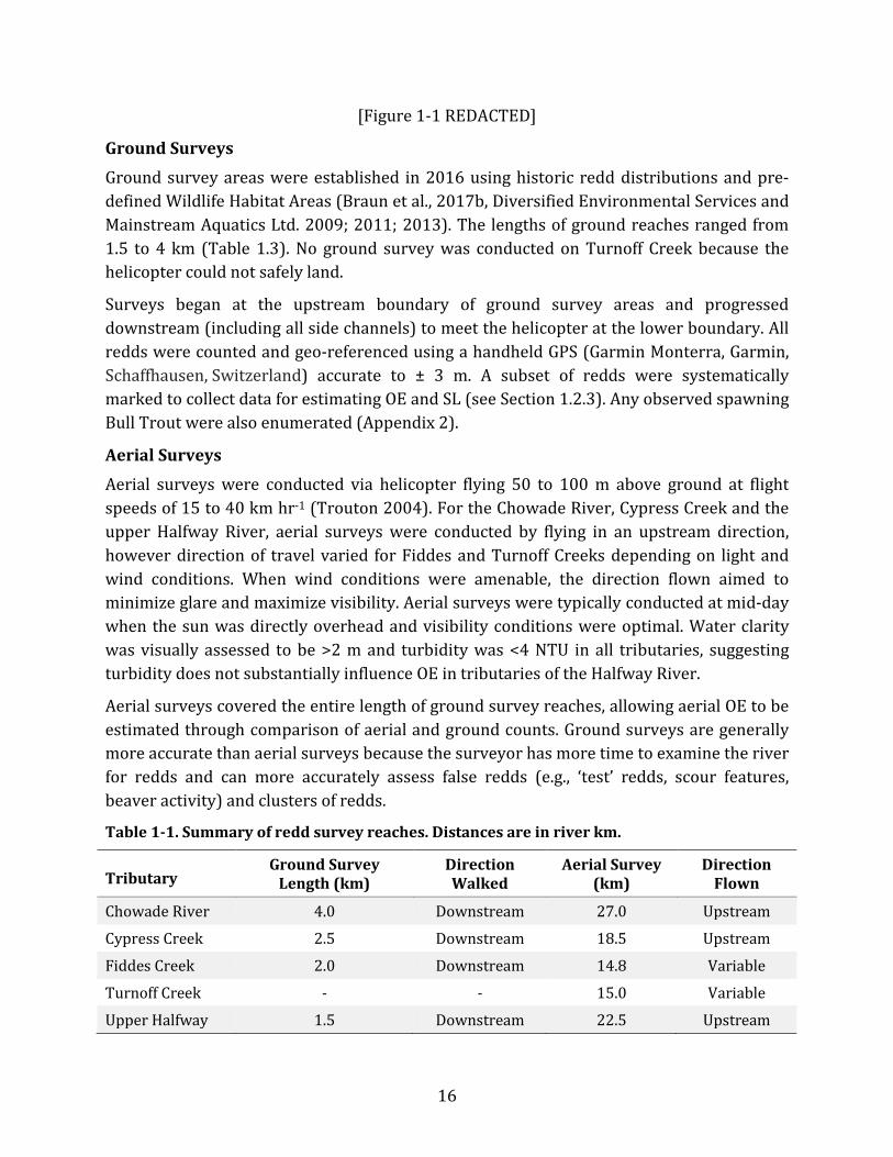
List of Tables Table 1-1. Summary of redd survey reaches. Distances are in river km. ..................................... 16

Table 1-2. Ground counts, aerial counts, and observer efficiencies. Ground OEs for Surveys 2 through 4 are in parentheses. ........................................................................................................... 23

Table 1-3 Survey life (days) estimated using daily redd ages from wildlife camera data on four redds in the Chowade River. Four independent analysts assessed daily redd ages, which were then used to model survey life. ................................................................................... 25

Table 1-4. GAUC estimates for Bull Trout redd abundance. Observer efficiency (OE) and survey life (SL) means and standard errors (SE) are input parameters for the AUC models. The 95% confidence limits (CL) are the 2.5 and 97.5% confidence bounds. .... 27

Table 1-5. Current and baseline estimates of Bull Trout redd abundance. From 2002 to 2012, peak count estimates are provided, and for 2016 through 2018, GAUC and peak count estimates are presented. Surveys for peak counts varied in the length of stream surveyed and survey method among years within tributaries. NS denotes a year in which no surveys were conducted. .................................................................................................... 28

Table 1-6. Summary of predicted mean fork lengths and egg number from redd area by tributary using Equations 1.6, 1.7 and 1.8. Ranges are in parentheses. .............................. 32

Table 2-1. Description of the power system design for the Chowade River and Cypress Creek in 2018. ............................................................................................................................................. 38

Table 2-2. Definition of error rates used to classify counter records during validation. ....... 42

Table 2-3. Comparison of fish lengths estimated in the Chowade River through video validation in 2016 - 2018. All fish were identified to species in 2017 so no data exists in the small salmonids category. .............................................................................................................. 51

Table 2-4. Summary of counter accuracy data for Bull Trout on each counter channel, Chowade River 2018. ............................................................................................................................... 51

Table 2-5. Detection efficiency of the Chowade River and Cypress Creek (all species combined) PIT arrays when 2 antennas were operational. Numbers in parentheses represent the number of individuals detected by both antennas out of the total number of individuals known to have passed by the arrays. .................................................................... 63

Table 2-6. Comparison of fish lengths estimated in Cypress Creek through video validation in 2018. Note that the small salmonids were difficult to identify but also difficult to measure. ........................................................................................................................................................ 68

Table 2-7. Summary of counter accuracy data for Bull Trout on each counter channel, Cypress Creek 2017. ................................................................................................................................. 69

xii

Project Background BC Hydro developed the Site C Fisheries and Aquatic Habitat Monitoring and Follow-up Program (FAHMFP) in accordance with Provincial Environmental Assessment Certificate Condition No. 7 and Federal Decision Statement Condition Nos. 8.4.3 and 8.4.4 for the Site C Clean Energy Project (the Project). The Site C Reservoir Tributaries Fish Community and Spawning Monitoring Program (Mon-1b) represents one component of the FAHMFP and aims to determine the effects and effectiveness of mitigation measures of the Project on fish populations (and their habitat) that migrate to tributaries of the reservoir. A subcomponent of this program (Task 2b) assesses spawning populations of Bull Trout (Salvelinus confluentus) in the Halfway Watershed. Data collected for this task will be used to directly address the following management question and hypotheses:

How does the Project affect Peace River fish species that use Site C Reservoir tributaries to fulfil portions of their life history over the short (10 years after Project operations begin) and long (30 years after Project operations begin) terms?

H0: There will be no change in Bull Trout spawner abundance in the Halfway River relative to baseline estimates.

H1: Bull Trout spawner abundance in the Halfway River will decline by 20 to 30% relative to baseline estimates.

The objective of the Peace River Bull Trout Spawning Assessment (Mon-1b, Task 2b) is to assess the abundance, timing, and distribution of Bull Trout spawning in the Halfway Watershed. Monitoring builds upon Bull Trout spawning assessments conducted prior to the construction of the Project, including aerial, ground, and snorkel surveys of redd abundance (2002-2012; Diversified Environmental Services and Mainstream Aquatics Ltd. 2009; 2011; 2013), and a fish fence operated in the Chowade River in 1994 (R.L. & L. Environmental Services LTD. 1995).

We improve upon historic redd count surveys by estimating redd abundance using a Gaussian area-under-the-curve (GAUC) methodology that accounts for uncertainty in visual observation while still generating peak count data comparable to historic indices. Resistivity counters in the Chowade River and Cypress Creek will provide independent estimates of spawn timing and spawner abundance, as well as additional data on movement of Bull Trout in the Halfway Watershed. The ratio of Bull Trout spawners to redds will be generated annually for the Chowade River and Cypress Creek, which can be used to interpret how changes in redd abundance relate to overall changes in Bull Trout spawning populations.

This report is separated into two chapters. Chapter 1 describes the Bull Trout redd abundance estimation, while Chapter 2 describes the operation of the resistivity counters and PIT arrays in the Chowade River and Cypress Creek.

13

1 Bull Trout Redd Abundance Estimation 1.1 Introduction Bull Trout population sizes have previously been assessed using redd count surveys in key spawning tributaries of the Halfway Watershed (Diversified Environmental Services and Mainstream Aquatics Ltd. 2009; 2011; 2013). Historically, redd counts in the Halfway Watershed combined aerial helicopter surveys, snorkel surveys, and stream walks to generate peak redd count indices. Unlike visual surveys that count the number of spawning adults, redd count surveys provide an index of effective population size (i.e., number of reproducing adults; Gallagher et al. 2007).

The main limitation of redd counts is their subjective nature, which relies on the ability of each surveyor to minimize the error associated with their observations. The primary sources of error are: (1) observer efficiency (OE; the ratio of the number of redds observed versus the true number of redds present), (2) not accounting for redd survey life (SL; the length of time a redd can be detected or counted by an observer), (3) poor temporal coverage of surveys (too few surveys or surveys not covering the peak spawning period), (4) poor spatial coverage (only surveying likely spawning areas or areas convenient to access). There will be low confidence in population estimates if these sources of uncertainty are not accounted for and temporal and spatial coverage is poor.

Unlike peak count indices, AUC methods can incorporate OE and SL when estimating population abundance. This approach is widely used to estimate the number of spawners or redds in a river from visual count data (Hilborn et al. 1999). There are many versions of AUC models that employ a range of run- or spawn-timing models, estimation procedures (Holt and Cox 2008), and methods of incorporating uncertainty. For example, Millar et al. (2012) developed a GAUC approach using a normally-distributed timing model that is estimated using maximum likelihood and accounts for uncertainty in OE and SL. This approach outperformed other commonly used AUC approaches, and was robust to assumptions of a normal timing model when estimating Pink Salmon (Oncorhynchus gorbuscha) abundance (Millar et al. 2012).

In populations where female size varies, redd counts may not accurately represent the number of eggs deposited. For example, larger females produce more eggs (Kindsvater et al. 2016) and build larger redds (Riebe et al. 2014), contributing disproportionately to juvenile recruitment. Accounting for redd size could increase the reliability of redd estimates and provide a more direct link to juvenile data being collected under Mon-1b, Task 2c (Site C Reservoir Tributaries Fish Population Indexing Survey). Furthermore, redd size may provide information on the relative number of resident versus migratory Bull Trout in tributaries of the Halfway River. This could be achieved by directly linking female length and fecundity to redd size through coordination among FAHMFP programs that capture, tag, and track spawning Bull Trout.

14

The objective of the redd surveys is to standardize data collection methodologies and estimate redd abundance while minimizing and quantifying uncertainty. Accurate estimates of Bull Trout redd abundance will be achieved by incorporating uncertainty in OE and SL into GAUC models. In addition, increasing the number of redd surveys over longer time periods (relative to historic peak counts) will provide more reliable information on spawn timing and redd abundances. Finally, accounting for redd size will provide a more direct link to the number of eggs deposited in each tributary. This approach provides an increased ability to track changes in Bull Trout population size over time to inform effective mitigation measures for migratory Bull Trout moving upstream and downstream of the Project.

1.2 Methods 1.2.2 Visual Surveys

We performed weekly redd count surveys on Cypress Creek, the Chowade River, the upper Halfway River0F

1, Fiddes Creek, and Turnoff Creek over a four-week period [REDACTED] (Figure 1-11 F

2, Appendix 1). We also performed a single aerial and ground survey in Needham Creek [REDACTED] to generate a peak redd count for this tributary. Inclement weather during the first week of surveys inhibited helicopter operation, and the Chowade River was the only tributary surveyed. In Cypress Creek and the upper Halfway River, all four surveys occurred [REDACTED].

During each survey, two experienced biologists conducted helicopter-assisted redd counts consisting of aerial surveys in all known spawning reaches (Table 1-1) and ground surveys in high-density spawning reaches. Aerial and ground survey reaches were laid out during reconnaissance surveys by InStream Fisheries Research Inc. in 2016 (Braun et al., 2017b) and radio telemetry studies performed in the mid-2000s (Diversified Environmental Services and Mainstream Aquatics Ltd. 2013 and references therein).

Redds were identified as areas with disturbed and cleaned substrate, with an obvious crest at the upstream end of the disturbed area, a tailspill area where disturbed substrate gathered, and a distinct depression between the crest and tailspill (Gallagher et al. 2007). These criteria were confirmed by periodic observations of active spawning during both aerial and ground surveys. Bull Trout redds were often found in overlapping clusters, and the number of redds per cluster was defined as the number of crest-tailspill pairs. While all redd criteria were visible during ground surveys, patches of disturbed and cleaned substrate were the primary characteristics used to identify redds during aerial surveys.

1 We define the upper Halfway River as the portion of the Halfway River from its source to the confluence of the Halfway and Graham Rivers. 2 All map images were created in R (R Core Team 2017) using packages rgdal (Bivand et al. 2017), GISTools (Brundson and Chen 2014), and sp (Bivand et al. 2013).

15

[Figure 1-1 REDACTED]

Ground Surveys Ground survey areas were established in 2016 using historic redd distributions and pre-defined Wildlife Habitat Areas (Braun et al., 2017b, Diversified Environmental Services and Mainstream Aquatics Ltd. 2009; 2011; 2013). The lengths of ground reaches ranged from 1.5 to 4 km (Table 1.3). No ground survey was conducted on Turnoff Creek because the helicopter could not safely land.

Surveys began at the upstream boundary of ground survey areas and progressed downstream (including all side channels) to meet the helicopter at the lower boundary. All redds were counted and geo-referenced using a handheld GPS (Garmin Monterra, Garmin, Schaffhausen, Switzerland) accurate to ± 3 m. A subset of redds were systematically marked to collect data for estimating OE and SL (see Section 1.2.3). Any observed spawning Bull Trout were also enumerated (Appendix 2).

Aerial Surveys Aerial surveys were conducted via helicopter flying 50 to 100 m above ground at flight speeds of 15 to 40 km hr-1 (Trouton 2004). For the Chowade River, Cypress Creek and the upper Halfway River, aerial surveys were conducted by flying in an upstream direction, however direction of travel varied for Fiddes and Turnoff Creeks depending on light and wind conditions. When wind conditions were amenable, the direction flown aimed to minimize glare and maximize visibility. Aerial surveys were typically conducted at mid-day when the sun was directly overhead and visibility conditions were optimal. Water clarity was visually assessed to be >2 m and turbidity was <4 NTU in all tributaries, suggesting turbidity does not substantially influence OE in tributaries of the Halfway River.

Aerial surveys covered the entire length of ground survey reaches, allowing aerial OE to be estimated through comparison of aerial and ground counts. Ground surveys are generally more accurate than aerial surveys because the surveyor has more time to examine the river for redds and can more accurately assess false redds (e.g., ‘test’ redds, scour features, beaver activity) and clusters of redds.

Table 1-1. Summary of redd survey reaches. Distances are in river km.

Tributary Ground Survey

Length (km) Direction Walked

Aerial Survey (km)

Direction Flown

Chowade River 4.0 Downstream 27.0 Upstream

Cypress Creek 2.5 Downstream 18.5 Upstream

Fiddes Creek 2.0 Downstream 14.8 Variable

Turnoff Creek - - 15.0 Variable

Upper Halfway 1.5 Downstream 22.5 Upstream

16

River

Needham Creek 2.2 Downstream 8.1 Upstream

1.2.3 Redd Marking

During ground surveys, redds were marked by inserting a green bristle tag with a 12-inch stake into the crest of the redd. A small label containing a unique redd number was attached to each tag and redds were tracked throughout the spawning period. When a redd was no longer identifiable, the tag was removed and the redd was not enumerated. All accessible redds were marked during ground surveys to maximize the accuracy of ground OE. For each redd, the unique redd identifier (redd tag number) was recorded along with the date, GPS location, age class, and whether the redd was observable (Gallagher et al. 2007). Redd length and width were measured to the nearest centimeter. Length was defined as the distance between the upper crest of disturbed substrate to the end of the tailspill, and width was the distance of disturbed substrate measured perpendicular to the length axis.

1.2.4 Redd Abundance Observer Efficiency

Ground observer efficiency was estimated for each survey by dividing the number of marked redds observed by the number of marked redds available to be observed (similar to mark-recapture methods; Melville et al. 2015). The number of observed redds was expanded to a redd abundance estimate for each ground survey reach by dividing the number of observed redds by the mean ground survey OE. A key assumption was that there was no tag loss; this was assessed by deploying 10 test tags annually in each tributary and determining whether tags were lost over the survey period (no tags were lost in 2016 through 2018). Test tags were deployed in areas with substrate and flow characteristics suitable for Bull Trout spawning.

To estimate aerial OE, we compared aerial redd counts within the ground reach boundaries to the ground redd counts estimated using the ground OE. For example, if ground surveys counted 12 redds and the ground OE was 0.75, the estimated redd abundance in the ground reach would equal 16. If 8 redds were observed during the aerial survey over the ground reach, the aerial OE would be calculated as 8/16 = 0.5. This method for calculating OE for aerial surveys is novel and combines conventional methods for estimating OE. Ground surveys were not conducted on Turnoff Creek and we used OE values from Fiddes Creek (with similar substrate and flow characteristics) during GAUC estimation. Aerial OE was very low for Cypress Creek in 2018, but field observations suggested that the estimates were not representative of the entire tributary; the aerial OE from the Chowade River was used for Cypress Creek during GAUC estimation.

17

Survey Life Survey life (the number of days a redd is observable and available to be counted) was estimated by tracking the age class of marked redds over consecutive ground surveys. We determined SL during ground surveys and applied this SL to aerial surveys during GAUC estimation. Redd age class was recorded following the methods of Gallagher et al. (2007):

Age-0 = the date the redd was first constructed (not measurable during surveys);

Age-1 = new since last survey but clear (the first measurable age class);

Age-2 = still measurable but already measured, negligible periphyton growth;

Age-3 = no longer measurable but still apparent, periphyton growth apparent;

Age-4 = no redd apparent, only a tag (at which point the tag will be removed); and

Age-5 = poor conditions; cannot determine if present and measurable or not.

We estimated average SL across all surveyed tributaries using a linear mixed effects model of survey date versus redd age class, fit using restricted maximum likelihood. The linear model related normalized survey day (day 1 was the day each redd was first observed and tagged) to the assigned redd age class. We defined SL as the predicted normalized survey day at which redds became age-4, or no longer apparent. As random effects we added intercepts for each tag ID and allowed by-tag ID random slopes for the effect of redd age class. The redd age class model for predicting the normalized survey day was:

(1.1) 𝑦𝑦𝑖𝑖~𝑁𝑁�𝛼𝛼𝑗𝑗[𝑖𝑖] + 𝛽𝛽𝑗𝑗[𝑖𝑖]𝑟𝑟𝑟𝑟𝑟𝑟𝑟𝑟_𝑎𝑎𝑎𝑎𝑟𝑟𝑖𝑖,𝜎𝜎𝑦𝑦2� 𝑓𝑓𝑓𝑓𝑟𝑟 𝑖𝑖 = 1 …𝑁𝑁

where 𝛼𝛼𝑗𝑗[𝑖𝑖] and 𝛽𝛽𝑗𝑗[𝑖𝑖] are normally distributed intercept and slope parameters incorporating random variation for each tag ID j (i represents the sample number). All linear mixed effects modelling was performed in R (R Core Team 2017) using lme4 (Bates et al. 2015).

Survey life can be specific to individual tributaries as a result of unique physical and biological stream characteristics (e.g., substrate, flow, periphyton growth, etc), and examining the effect of tributary on SL modelling is important for understanding redd ageing throughout the Halfway Watershed. Due to the complex nature of redd ageing and the increased data requirements when incorporating fixed effects into linear mixed effects models (i.e., adequate samples sizes for each tributary), we will delay the use of tributary-specific SL in AUC modelling. Tributary-specific survey life and other candidate model formulations will be explored during synthesis modelling, and annual redd abundance estimates can be adjusted accordingly.

Trail Cameras

We installed trail cameras (Defender 850, Browning, Morgan, Utah, USA) with polarizing filters on five redds in the Chowade River [REDACTED] to verify SL assumptions and

18

examine Bull Trout spawning behaviour. While redd age was assessed only once per week during ground surveys, the trail cameras provided daily redd ages that could be used to determine the exact day a redd progressed in age. We installed the cameras on age-1 redds with active Bull Trout spawning behaviour. Time lapse photos were taken each hour for the entire survey period, and additional photos were taken when the camera’s motion-sensing feature was triggered. Trail cameras monitored redds for 14 days before being removed during the final ground survey [REDACTED].

A single, clear image was selected from each redd on each day, and four analysts independently estimated daily redd age. To account for the continuous nature of redd ageing, half ages were sometimes used to describe transitional periods that were difficult to categorize. We performed linear regressions of survey date versus daily redd age to compare predicted SL (for each analyst and for the average of the four analysts) to average SL estimated using Equation 1.1.

GAUC Estimates We used a GAUC method to generate a redd abundance estimate for each tributary. In this method, visual fish stock assessment data are modelled using a quasi-Poisson distribution with spawn-timing described by a normal distribution, and parameter estimates evaluated using maximum likelihood estimation (described in Millar et al. 2012). For our analysis, spawn-timing was defined as the timing of new redd establishment throughout the spawning season. The advantages of this GAUC approach over conventional AUC and peak count indices is the ability to incorporate variance in OE and SL, fit spawn-timing using maximum likelihood estimation, and estimate the uncertainty in redd abundance.

With abundance modelled as a quasi-Poisson distribution with normally distributed spawn-timing (Millar et al. 2012), the number of observed redds at time t (Ct) is

(1.2) 𝐶𝐶𝑡𝑡 = 𝑎𝑎 𝑟𝑟𝑒𝑒𝑒𝑒 �−(𝑡𝑡 − 𝑚𝑚𝑠𝑠)2

2𝜏𝜏𝑠𝑠2�

where a is the maximum height of the redd count curve, ms is the time of the peak number of redds, and 𝜏𝜏𝑠𝑠2 is the standard deviation of the arrival timing curve. Because the normal density function integrates to unity, the exponent term in Equation 1.2 becomes �2𝜋𝜋𝜏𝜏𝑠𝑠 and Equation 1.2 can be simplified to

(1.3) 𝐶𝐶𝑡𝑡 = 𝑎𝑎�2𝜋𝜋𝜏𝜏𝑠𝑠

A final estimate of abundance (Ê) is obtained by applying OE (v) and SL (l) to the estimated number of observed redds (or fish-days: 𝐹𝐹�𝐺𝐺)

19

(1.4) 𝐸𝐸� =𝐹𝐹�𝐺𝐺𝑙𝑙 ∗ 𝑣𝑣

Ê in Equation 1.4 is estimated using maximum likelihood (ML), where 𝑎𝑎� and �̂�𝜏 are the ML estimates of a and 𝜏𝜏𝑠𝑠 in Equation 1.3 (�̂�𝐶𝑡𝑡 = 𝑎𝑎��2𝜋𝜋�̂�𝜏𝑠𝑠).

The GAUC estimation in Equation 1.3 can be re-expressed as a linear model, allowing the estimation to be performed as a simple log-linear equation with an over-dispersion correction factor. The over-dispersion correction accounts for instances where the variance of the redd observations exceeds the expected value. The number of fish-days (𝐹𝐹�𝐺𝐺 , representing the number of observed redds) can be estimated using

(1.5) 𝐹𝐹�𝐺𝐺 = �

𝜋𝜋−�̂�𝛽2

𝑟𝑟𝑒𝑒𝑒𝑒 �𝛽𝛽0 −�̂�𝛽12

4�̂�𝛽2�

where 𝛽𝛽0, 𝛽𝛽1, 𝛽𝛽2 are the regression coefficients of the log-linear model. Uncertainty in OE and SL are incorporated into the estimated redd abundance using the covariance matrix of the modeled parameters (𝛽𝛽0, 𝛽𝛽1, 𝛽𝛽2) via the delta method (described in Millar et al. 2012).

Mean abundance estimates and input parameters are presented along with standard error, 2.5% and 97.5% confidence limits, and percent relative uncertainty (%RU), calculated as

(1.6) %𝑅𝑅𝑅𝑅 = �

|𝑢𝑢 − SE|𝑢𝑢

� ∙ 100

where 𝑢𝑢 is the mean abundance estimate, 𝑆𝑆𝐸𝐸 is the standard error of the mean, and the vertical lines indicate the absolute value.

We examined the effect on GAUC estimation of adding zero counts to the beginning and end of the spawning period (Appendix 3). An initial zero count was added one week before the first survey, and a final zero count was added to the date equal to the number of days estimated as the redd survey life after the last new redd was observed (e.g., if the last age-1 redd was observed during Survey 3 and SL was 14 days, the final zero would be 14 days after Survey 3). This ensured that the last redds observed during surveys would not be observable on the zero-count date.

To continue historic peak count indices from 2002 to 2012, we calculated a peak count index for each tributary following the methods described in Diversified Environmental Services and Mainstream Aquatics Ltd. (2013). Historic redd counts were conducted during one or two survey weeks [REDACTED] (Diversified Environmental Services and Mainstream Aquatics Ltd. 2011, 2013). Each reach of the river was surveyed using one of three survey methods: (1) aerial, (2) ground, and/or (3) snorkel. The peak count index was

20

calculated for each tributary by adding redds that were observed on the first survey but not on the second survey to the total number of redds counted during the second survey. To generate a peak count comparable to historic methods, we summed the total number of redds observed during ground surveys with aerial counts that occurred outside of the ground survey reach for surveys [REDACTED] (i.e., the historic survey period)2F

3. Due to the spacing of our surveys, the peak count generally included data from one survey week (e.g., Survey 2 in 2018).

1.2.5 Redd Area, Predicted Spawner Size, and Fecundity

We measured the length and width of all redds marked during ground surveys to the nearest centimeter. Redd area was calculated assuming an elliptical shape:

(1.7) 𝐴𝐴 = 𝜋𝜋𝜋𝜋𝜋𝜋

where 𝐴𝐴 is the area of the disturbed stream bed, 𝜋𝜋 is the length of the redd measured from the crest to the tailspill, and 𝜋𝜋 is the maximum width of the disturbed stream bed perpendicular to the length axis.

We predicted fork-length from measured redd area using the redd area-fork length relationship defined in Riebe et al. (2014), which compared redd area and fork length for three species of Pacific salmon (Sockeye [O. nerka], Pink, and Chinook Salmon [O. tshawytscha]). The relationship between redd area and fork length was estimated as

(1.8) 𝐴𝐴 = 3.3 �𝜋𝜋

600�2.3

where A is redd area in m2, L is the female fork length in mm and 600 is a reference value that was near the average length of individuals in Riebe et al. (2014). The model was highly significant with a correlation coefficient (r) of 0.89 and a p-value <0.001 (n = 60).

The redd area equation was transformed to solve for fork length:

(1.9) 𝜋𝜋 = �6002.3A

3.3�0.434783

Published data on Bull Trout lengths and egg number were used to determine the length-fecundity relationship. Data were extracted from a review of Bull Trout life histories by McPhail and Baxter (1996), which included length and egg number data for six populations (Figure 1-2). The equation for the regression line used to estimate egg number was

(1.10) ln(𝐸𝐸) = −8.434 + 2.606ln(L)

3 In 2018 we extended this date range to September 21 to estimate a peak count index for Needham Creek.

21

where E is the number of eggs per female and L is the female’s fork length in millimeters.

Figure 1-1. Published data of Bull Trout female fork length by egg number. Both axes are on the natural log scale. The model R2 was 0.94 and the p-value was <0.0001.

1.3 Results 1.3.1 Redd Distribution

We examined redd distributions to assess Bull Trout spawning behaviour, identify high-quality spawning habitat, and verify that ground surveys were performed in areas of adequate redd abundance. Survey-specific redd distributions for the Chowade River, Cypress Creek, Fiddes Creek, Turnoff Creek, Needham Creek, and the upper Halfway River are shown in Figure 1-3 through Figure 1-6. For all tributaries with ground surveys (i.e., the blue areas in Figure 1-3 through Figure 1-6), ground survey reaches were located within areas of adequate redd density for generating observer efficiency estimates.





22

1.3.2 Redd Abundance Observer Efficiency

Ground observer efficiencies were calculated from the re-sighting of marked redds in all tributaries except in Turnoff Creek, where ground surveys were not conducted. Observer efficiency for ground surveys was estimated for Surveys 2, 3, and 4, and were relatively high and consistent among surveys and within tributaries (Table 1.4). Ground OE was >70% for all four tributaries, while aerial OE was highly variable and ranged from 0.0 to 1.0. Mean aerial OE was relatively consistent in the Chowade River (0.52, coefficient of variation [CV] 55%), Fiddes Creek (0.52, CV 34%), and the upper Halfway River (0.69, CV 33%), but was substantially lower and more variable in Cypress Creek (0.07, CV 138%). During ground surveys in Cypress Creek, redds were observed beneath log jams and under-cut banks, with few in the middle of the channel. Mid-channel redds were observed outside of the ground survey reach, suggesting that the aerial OE of 0.07 was not representative of the entire survey area. We used the aerial OE from the Chowade River to determine the GAUC abundance for Cypress Creek in 2018 to avoid overestimation of redd abundance.

The aerial OE for Needham Creek is likely biased low because we compared the aerial count to the ground count (rather than total ground reach abundance estimated by mark-recapture). Stream characteristics and the approximate OE value (0.24) for Survey 3 suggest survey conditions in Needham Creek may be similar to those in the Chowade River.

Table 1-2. Ground counts, aerial counts, and observer efficiencies. Ground OEs for Surveys 2 through 4 are in parentheses.

Tributary Number of

Redds Marked

Mean Ground OE Survey Ground

Count Total

Reddsa Aerial Countb Aerial OEc

Chowade River 50

0.87 (0.73, 0.93,

0.96)

1 11 11.9 11 0.92

2 42 45.5 13 0.29

3 58 62.8 23 0.37

4 54 58.4 28 0.48

Fiddes Creek 7 1.0

(1.0, 1.0, 1.0)

1 7 7 4 0.57

2 7 7 2 0.29

3 7 7 5 0.71

4 4 4 2 0.50

Upper Halfway River

27 1.0 (1.0, 1.0, 1.0)

1 11 11 11 1.00

2 26 26 12 0.46

3 31 31 21 0.68

4 29 29 18 0.62

23

Cypress Creek 15 0.93

(0.8, 1.0, 1.0)

1 5 5.2 1 0.19

2 13 13.5 1 0.07

3 15 15.6 0 0.00

4 7 7.8 0 0.00

Needham Creek - - 3 42 - 10 0.24d

a: Ground count / ground observer efficiency b: Aerial count within ground reach c: Aerial count / total redds d: We used aerial count/ground count to calculate OE for Needham Creek

Survey Life A total of 92 tags were applied to age-1 redds during ground surveys in Fiddes Creek, Cypress Creek, the Chowade River, and the upper Halfway River. Of these 92 tagged redds, 36% (33 redds) progressed to age-4 during the survey period (42% in the Chowade River, 57% in Cypress Creek, 50% in Fiddes Creek, and 12% in the upper Halfway River). The remaining tags were removed during the final survey at age-2 (8%, 7 redds), and age-3 (56%, 51 redds), and 1 redd (1%) was not re-sighted.

We estimated the mean SL for all redds in 2018 (including redds that did not progress to age-4) using a linear mixed effects model of normalized survey day versus age class (Figure 1-7). The optimal random effect structure was identified as random slope and random intercept for tag ID (ΔAIC from base model: 167.90; Appendix 4). The estimated SL was 18.5 days with a standard error of 2.15 days.

Figure 1-2. Redd age within all tributaries by normalized survey day, with points jittered for presentation. Black lines represent individual redds (i.e., shows random effect of redd ID).

24

Red line shows mean for all redds, and vertical error bars are the 95% confidence interval based on a normal approximation. Negative normalized survey days correspond to the number of days between the redd being built (age-0) and the first observation by surveyors. A normalized survey day of 1 is when the redd was first observed by surveyors. See Equation 1.1 for model details.

Trail Cameras Four of the five deployed wildlife trail cameras provided clear daily photographs of four redds in the Chowade River (see example in Appendix 5). Daily redd ages were used to model redd-specific and analyst-specific SL (Table 1.6; SL modelling for Analyst 1 is shown in Figure 1-8) and compared to SL estimated from redd survey data. Estimated SL for the four redds was similar among analysts, despite minor discrepancies between daily redd ages. The mean SL of all four redds across all analysts was 18.3 days (SD 4.2 days), similar to mean SL estimated using all redd survey data (18.5 days).

Table 1-3 Survey life (days) estimated using daily redd ages from wildlife camera data on four redds in the Chowade River. Four independent analysts assessed daily redd ages, which were then used to model survey life.

Redd Analyst 1 Analyst 2 Analyst 3 Analyst 4 Avg (SD)

Redd 1 17.4 16.0 21.0 22.0 19.1 (2.9) Redd 2 13.6 13.5 13.0 16.4 14.1 (1.5) Redd 3 13.5 14.3 21.0 16.0 16.2 (3.4) Redd 4 25.1 21.3 22.0 27.1 23.9 (2.7)

25

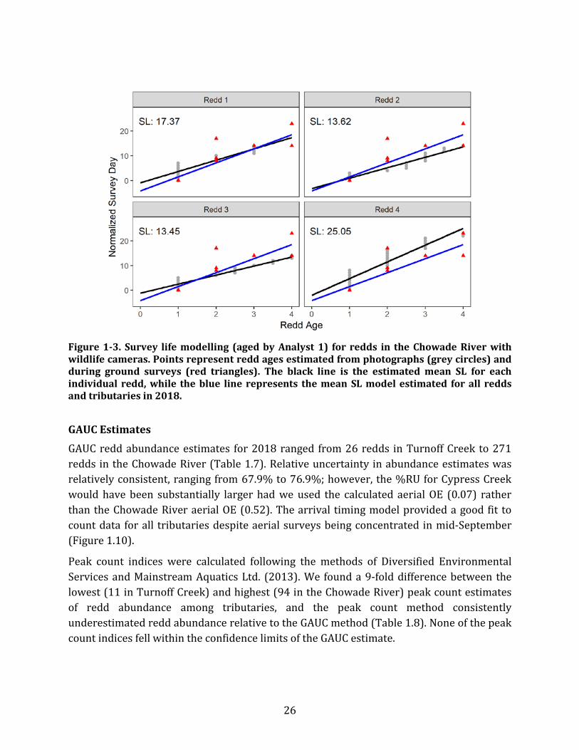
Figure 1-3. Survey life modelling (aged by Analyst 1) for redds in the Chowade River with wildlife cameras. Points represent redd ages estimated from photographs (grey circles) and during ground surveys (red triangles). The black line is the estimated mean SL for each individual redd, while the blue line represents the mean SL model estimated for all redds and tributaries in 2018.

GAUC Estimates

GAUC redd abundance estimates for 2018 ranged from 26 redds in Turnoff Creek to 271 redds in the Chowade River (Table 1.7). Relative uncertainty in abundance estimates was relatively consistent, ranging from 67.9% to 76.9%; however, the %RU for Cypress Creek would have been substantially larger had we used the calculated aerial OE (0.07) rather than the Chowade River aerial OE (0.52). The arrival timing model provided a good fit to count data for all tributaries despite aerial surveys being concentrated in mid-September (Figure 1.10).

Peak count indices were calculated following the methods of Diversified Environmental Services and Mainstream Aquatics Ltd. (2013). We found a 9-fold difference between the lowest (11 in Turnoff Creek) and highest (94 in the Chowade River) peak count estimates of redd abundance among tributaries, and the peak count method consistently underestimated redd abundance relative to the GAUC method (Table 1.8). None of the peak count indices fell within the confidence limits of the GAUC estimate.

26

Table 1-4. GAUC estimates for Bull Trout redd abundance. Observer efficiency (OE) and survey life (SL) means and standard errors (SE) are input parameters for the AUC models. The 95% confidence limits (CL) are the 2.5 and 97.5% confidence bounds.


Tributary GAUC

Abundance (SE)

2.5% CL

97.5% CL %RU Aerial OE

(SE) Survey Life

(SE)

Peak Count Index

Chowade River 271 (80) 151 484 70.5 0.52 (0.115) 18.50 (2.15) 94

Cypress Creek 53 (17) 28 101 67.9 0.52 (0.115) 18.50 (2.15) 52

Fiddes Creek 46 (13) 26 81 71.7 0.52 (0.071) 18.50 (2.15) 43

Turnoff Creek 26 (6) 16 42 76.9 0.52 (0.071) 18.50 (2.15) 23

Upper Halfway River

57 (14) 35 93 75.4 0.69 (0.092) 18.50 (2.15) 55

Needham Creek - - - - - - 50

27

Table 1-5. Current and baseline estimates of Bull Trout redd abundance. From 2002 to 2012, peak count estimates are provided, and for 2016 through 2018, GAUC and peak count estimates are presented. Surveys for peak counts varied in the length of stream surveyed and survey method among years within tributaries. NS denotes a year in which no surveys were conducted.

Peak Count Indices GAUC

Tributary 2002 2004 2007 2008 2010 2012 2016 2017 2018 2016 2017 2018

Chowade River 104 210 NS 425 864 321 108 116 94 290 320 271

Cypress Creek NS NS 17 120 60 62 33 38 23 90 90 53

Fiddes Creek NS NS NS NS 146 59 20 18 22 107 63 46

Turnoff Creek NS NS NS NS 56 40 9 3 11 44 18 26

Upper Halfway River NS NS 11 23 86 33 16 31 18 20 75 57

Needham Creek NS NS 29 78 103 80 NS NS 50 NS NS NS

28

1.3.3 Annual OE and GAUC

We compared OE and GAUC redd abundance among study years in the Halfway Watershed (Figure 1-10). The most stable GAUC estimates were in the Chowade River, while estimates for Fiddes Creek and the upper Halfway River were variable between years. Apart from Turnoff Creek, all GAUC estimates were lower in 2018 relative to 2017. Redd counts within ground survey reaches (not shown) were generally higher in 2018, suggesting shifts in redd distributions throughout the tributaries.

Ground OE was consistently high in all tributaries, but aerial OE was much lower and variable among years and tributaries (Figure 1.11). In Fiddes Creek and the Chowade River, aerial OE was slightly higher in 2018 relative to previous survey years. Aerial OE was similar between the Chowade River and Cypress Creek in 2017, but much lower in 2018 in Cypress Creek as OE was biased low. The similarities between the Chowade River and Cypress Creek in 2017 provide further justification to use the aerial OE from the Chowade River to determine the GAUC abundance for Cypress Creek in 2018.

Figure 1-4. Mean aerial OE, ground OE, and GAUC estimates (error bars represent 95% confidence intervals) in the Halfway Watershed from 2016 to 2018.

29

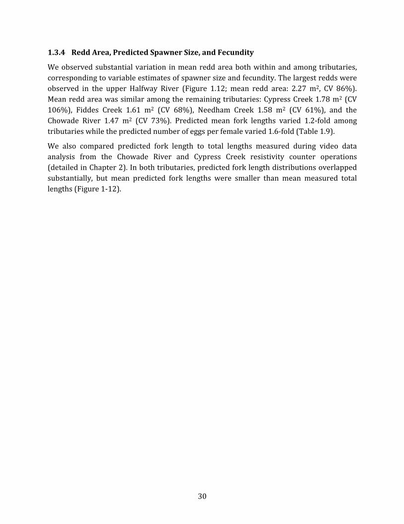
1.3.4 Redd Area, Predicted Spawner Size, and Fecundity

We observed substantial variation in mean redd area both within and among tributaries, corresponding to variable estimates of spawner size and fecundity. The largest redds were observed in the upper Halfway River (Figure 1.12; mean redd area: 2.27 m2, CV 86%). Mean redd area was similar among the remaining tributaries: Cypress Creek 1.78 m2 (CV 106%), Fiddes Creek 1.61 m2 (CV 68%), Needham Creek 1.58 m2 (CV 61%), and the Chowade River 1.47 m2 (CV 73%). Predicted mean fork lengths varied 1.2-fold among tributaries while the predicted number of eggs per female varied 1.6-fold (Table 1.9).

We also compared predicted fork length to total lengths measured during video data analysis from the Chowade River and Cypress Creek resistivity counter operations (detailed in Chapter 2). In both tributaries, predicted fork length distributions overlapped substantially, but mean predicted fork lengths were smaller than mean measured total lengths (Figure 1-12).

30

Figure 1-5. Frequencies of redd area by tributary. Insets represent the shape of redds based on lengths and widths and an assumed elliptical shape. Redds are centered at the origin of the inset plots (0,0).

31

Figure 1-6. Probability density functions for fork lengths predicted from redd area data and total lengths measured during video analysis at the Chowade River and Cypress Creek resistivity counter sites in 2018.

Table 1-6. Summary of predicted mean fork lengths and egg number from redd area by tributary using Equations 1.6, 1.7 and 1.8. Ranges are in parentheses.

Tributary Fork Length (mm) Egg Number

Chowade River 422 (226-695) 1510 (297-5540)

Cypress Creek 459 (234-801) 1879 (325-8019)

Fiddes Creek 439 (202-600) 1673 (221-3777)

Upper Halfway River 510 (165-811) 2473 (131-8283)

Needham Creek 436 (226-662) 1644 (297-4880)

1.4 Discussion 1.4.1 Redd Abundance

We used a GAUC method to estimate 2018 redd abundance in five tributaries of the Halfway Watershed. This monitoring builds upon GAUC estimates from 2016 and 2017 (Braun et al. 2017b; Putt et al. 2018) and intermittent historic peak counts from 2002 to 2012 (Diversified Environmental Services and Mainstream Aquatics Ltd. 2009; 2011;

32

2013). The GAUC method improves upon peak count indices as it incorporates error in OE and SL and produces a full redd abundance estimate (as opposed to an index of abundance). Despite poor weather conditions in 2018 that disrupted helicopter flights and reduced aerial visibility, the GAUC method produced complete redd abundance estimates with relative uncertainties only slightly higher relative to 2016 and 2017 estimates. Results from 2018 suggest the GAUC method is robust to poor survey conditions that might disrupt or prevent historic peak count methods.

Uncertainty in GAUC abundance estimates can be attributed to error in OE, SL, and the spatial and temporal coverage of redd surveys, and understanding and quantifying these sources of error is integral to producing an accurate and precise redd abundance estimate. Ground OE has been consistently high in all tributaries in all survey years (2016 to 2018), which agrees with literature suggesting detailed ground surveys are an accurate redd counting method (Dunham et al 2001). The high OE in ground surveys justifies our use of ground counts to verify aerial counts and determine aerial OE.

Compared to ground OE, aerial OE was lower and varied by tributary in all study years. Variability in aerial OE is expected given tributary-specific river conditions (flow, temperature, turbidity), visual survey conditions (water depth, clarity, and glare), helicopter survey conditions (e.g., glare, survey height, and survey speed) and redd distributions. Aerial OE was low in 2018 compared to previous years and varied by both tributary and survey date, possibly due to poor visibility during aerial surveys driven by wind and rain that resulted in faster and higher flight paths. Lower aerial OE may also have been related to redd distribution patterns. For example, in Cypress Creek a greater proportion of redds in the ground survey reach were located along the tributary margins (relative to previous years), making the redds more difficult to see from the air and thereby reducing aerial OE. Variability in aerial OE can contribute substantially to overall uncertainty in the GAUC estimates, and additional years of OE data will inform the range in aerial OE for all tributaries, particularly those with fewer redds.

Survey life also contributes to GAUC estimates and provides information on the degree of double counting across visual surveys (i.e., the same redd is counted during successive surveys). Field observations and linear mixed effects modelling suggest that SL in the Halfway Watershed may be variable among years, tributaries, and within tributaries. We used several analytical methods to estimate SL, including linear modelling of redd data, calculating individual SL for redds that progressed from one to four (minimum SL as the period from age-0 to age-1 is not accounted for), and analyzing daily wildlife camera photos. The results of these methods were relatively consistent and indicate that variation in SL is likely related to tributary characteristics (e.g., flow, temperature, and productivity), rather than analysis method.

33

Redd surveys in 2018 were concentrated within a shorter time window relative to previous years, which may have contributed to higher relative uncertainties in GAUC abundance estimates. [REDACTED]. Aerial survey counts in Fiddes, Turnoff and Cypress creeks were clustered near the peak count and the GAUC model could not estimate redd abundance without the addition of at least one zero at either the beginning or end of the survey period (Appendix 3). Results from previous years found that the addition of zeros at the beginning and end of the time series did not substantially affect the GAUC estimate, justifying the addition of zeros in 2018. Although performing surveys throughout the entire Bull Trout spawning period is important for maximizing accuracy and precision of redd abundance estimates, the results from 2018 demonstrate the robustness of the GAUC method to missing data and challenging survey conditions.

Peak redd count indices for Cypress Creek and the upper Halfway River in 2016 through 2018 were within the range of baseline surveys from 2002 to 2012, while peak counts in the Chowade River, Fiddes Creek, and Turnoff Creek were low relative to baseline indices. The rank order of peak counts was similar between 2002-2012 and 2016-2018, with the Chowade River consistently having the highest peak count. Needham Creek had the second highest peak count in 2018, indicating it is an important spawning tributary despite its short length (~8 km of accessible stream length). We found that peak count indices were sensitive to which surveys, and how many surveys, were included in the peak spawning window. This sensitivity highlights the uncertainty inherent in peak counts and suggests GAUC estimates are a more accurate and consistent method of redd abundance estimation.

The GAUC method provides a more accurate, precise, and informative abundance estimate relative to historic peak count methods. A power analysis by Ma et al. (2015) suggested that high rates of process error (i.e., natural variation in population size) in the Halfway Watershed may limit the ability to detect a decline in redd abundance, and only a small increase in power would occur if sampling error was reduced to zero. The power analysis assumed that redd estimates were accurate but imprecise, but previous research suggests redd count accuracy can be affected by stream characteristics, redd density, count frequency, and the skill of observers (Howell and Sankovich 2012; Al-Chokhachy et al. 2005; Dunham et al. 2001). The GAUC method provides an accurate, precise, and informative abundance estimate, which will maximize the probability of detecting a decline in Bull Trout abundance. Further, GAUC parameters for migration timing, observer error, and survey life could be used to improve the utility of historic redd abundance estimates and enhance models estimating changes in Bull Trout redd abundance through time.

1.4.2 Redd Area, Fish Length and Fecundity

Redd abundance can be a reliable indicator of Bull Trout spawning abundance (Gallagher et al. 2007), but may not be an accurate indicator of egg deposition and juvenile recruitment. Redd size is strongly correlated with fish length (Riebe et al. 2014), and because of the

34

strong length-fecundity relationships present in salmonids (Kindsvater et al. 2016), redd size is also correlated with the number of eggs a female deposits. Changes in redd abundance may not reflect changes in overall Bull Trout abundance if spawner size distributions do not remain relatively constant. In particular, large spawners can contribute disproportionately to juvenile recruitment relative to smaller spawners.

We estimated fork lengths for Bull Trout spawners in the tributaries of the Halfway Watershed using a literature relationship between redd area and fork length (Riebe et al. 2014). Bull Trout fork lengths estimated from redd areas were smaller than total lengths observed crossing the resistivity counter in the Chowade River and Cypress Creek in 2018. In Cypress Creek, mean fork length and mean total length were within 40 mm of each other, but in the Chowade River the mean total length was almost 200 mm larger than the mean fork length. The estimated mean fork length for the Chowade River (422 mm, range 226-695 mm) was also smaller than mean fork lengths measured during angling surveys in the Chowade River in 1994 and 1995 (Baxter 1997; female: 609.75 mm, range ~400-800 mm; male 630.03 mm, range ~300-900 mm), and fork lengths obtained during fish fence monitoring in 1994 (R. L. and L. Environmental Services Ltd. 1995; 604 mm, range 370-905 mm). Comparisons between fork lengths estimated from redds and forks lengths measured directly during current and historic studies suggests that the relationship between redd area and fork length from Riebe et al. (2014) may underestimate fork lengths for Bull Trout in tributaries of the Halfway Watershed.

We estimated fecundity for spawning Bull Trout in tributaries of the Halfway Watershed using literature relationships between fork length and fecundity (McPhail and Baxter 1996). The predicted fecundities show that larger female Bull Trout could potentially contribute thousands more eggs and potential recruits to the Halfway Watershed populations relative to smaller individuals. We acknowledge that the fecundity estimates presented herein are coarse calculations; however, the large variation in fecundity could affect juvenile recruitment and population dynamics in future years, particularly if Bull Trout size distributions are affected by the construction and operation of the Project.

35

2 Resistivity Counter and Passive Integrated Transponder Arrays in the Chowade River and Cypress Creek

2.1 Introduction Bull Trout population estimates in the Halfway Watershed have been generated using visual surveys of redds from 2002 to 2012 (peak count indices; Diversified Environmental Services and Mainstream Aquatics Ltd. 2009; 2011; 2013), and from 2016 through 2018 (AUC abundance estimates; Braun et al. 2017b, Putt et al. 2018). Although visual surveys can provide precise estimates of redd abundance and can monitor changes in abundance over time, redd abundance may not correlate directly with spawner abundance (Dunham et al. 2001, Gallagher and Gallagher 2005). It is important to understand the relationship between redd and spawner abundances to accurately monitor changes in Bull Trout populations over time.

Enumerating adult Bull Trout with resistivity counters and PIT arrays can provide independent estimates of spawner abundance, migration timing, spawning duration, stage-specific survival and transition probabilities (i.e., juvenile to subadult, subadult to adult), and fish size. Resistivity counters detect a fish movement when a fish swims over the counter and causes a change in electrical resistance. The change in resistance is measured by the counter and an algorithm is used to determine if a fish passed by the counter in an upstream or downstream direction. Resistivity counters can be up to 90% accurate for enumerating salmonids (Braun et al. 2016, Casselman et al. 2015), and are cost-effective, low maintenance, and can be applied to a variety of stream characteristics. PIT telemetry uses arrays of antennas (two or more antennas that provide directionality) that detect passive tags implanted into fish at a variety of life stages. PIT arrays can be an effective method for tracking migration behaviour, growth, and survival (Brännäs et al. 1994), and allow for monitoring and tracking of individual fish throughout their life cycle.

We enumerated spawning Bull Trout using resistivity counters and PIT arrays in the Chowade River and Cypress Creek in 2018. Resistivity counters enumerated Bull Trout spawners and collected information on direction of movement, migration timing, spawning duration, and the size of spawners. PIT arrays detected Bull Trout and Rainbow Trout (O. mykiss) tagged by other monitoring programs as they moved past the counter sites, and helped to inform migration patterns and spawn timing of adult and juvenile salmonids in the Chowade River and Cypress Creek.

2.2 Methods We used resistivity counters, video cameras, and PIT arrays to monitor fish movement in the Chowade River and Cypress Creek from early-August to early October. Resistivity counters monitored upstream and downstream movements of fish past the site, while the video cameras continuously monitored the counter pads to enable validation of the counter

36

data. Two-antenna PIT arrays were installed at each site to detect the directional movements of PIT-tagged Bull Trout and Rainbow Trout moving upstream or downstream.

2.2.1 Study Sites The Chowade River and Cypress Creek are both tributaries of the Halfway River. The Chowade River is a fifth order stream with a mainstem length of 87.1 km, and has resident populations of Bull Trout, Rainbow Trout, Arctic Grayling (Thymallus arcticus), Mountain Whitefish (Prosopium williamsoni) and Slimy Sculpin (Cottus cognatus). Cypress Creek is also a fifth order stream with similar resident fish populations to the Chowade River, and has a mainstem length of 81.7 km. In the Chowade River, the counter site is located 21.7 river kilometers (rkm) upstream of the Halfway River confluence, while in Cypress Creek the counter site is 16.9 rkm upstream of the Halfway River confluence (Figure 1-1). Resistivity counter sites were selected for their ease of access for equipment installation, suitable stream characteristics (e.g., flow, substrate size) for counter and PIT operation, and their location downstream of known Bull Trout spawning (Diversified Environmental Services and Mainstream Aquatics Ltd. 2009; 2011; 2013).

Adult Bull Trout typically migrate upstream past the counter sites in the Chowade River and Cypress Creek from mid-July to early September, and their downstream migration occurs from late August to early October (R.L. & L. Environmental Services Ltd. 1995, Braun et al. 2017a). In 2018, the resistivity counter and PIT array was operational from August 16 to October 2 in the Chowade River, and August 9 to October 1 in Cypress Creek, and therefore a substantial portion of the upstream migration was not monitored. The counters could not be installed in mid-July due to a storm event. Although all reasonable effort was made to install the counters prior to the onset of Bull Trout migration, high July flows related to storms and the tail-end of freshet delayed counter installation. Despite this delay, each year of counter operation will generate a full kelting (downstream) estimate that can be used as a reasonable index of spawner abundance. An upstream migration abundance and a ratio of upstream abundance to downstream abundance will be generated in years when flows permit counter installation in mid-July.

2.2.2 Environmental Conditions

Water depth was constantly recorded at each site using paired level loggers (HOBO U20, Onset Computer Corporation, Bourne, MA, USA). One logger was installed in a stilling well within the wetted stream width to record stage height, while another onshore logger recorded ambient air pressure (used to calibrate the stream logger). Discharge and water level data for a hydrometric station in the Halfway River (Station No: 07FA003) located downstream of the confluence between the Chowade River and the Halfway River were provided by the Water Survey of Canada. We examined the relationship between Halfway River discharge and water depth at each counter site using Pearson’s correlation coefficients (r). A strong relationship (high r value) would suggest that discharge in the

37

Halfway River could be used to approximate water depth at the counter sites, informing pre-season planning (e.g., installation dates) and in-season counter management (e.g., site visit timing, potential data gaps).

2.2.3 Remote Power Systems

The resistivity counter, video validation equipment, and PIT arrays at each counter site were powered by four separate battery banks paired with solar panels (Figure 2-1 and Table 2-1). Separate battery banks enabled us to maintain consistent power to high-priority equipment, specifically the resistivity counters and PIT arrays. Each battery bank was designed to supply sufficient power for a minimum of seven days, independent of solar power generation, and solar panels provided surplus power for re-charging battery banks. We determined the appropriate number of batteries and solar panels required for each power system using a conservative estimate of four hours of solar radiation per day. A back-up generator was located at each site and was used to re-charge batteries during extended periods of poor solar conditions.

In 2017, the power systems and solar charge controllers caused noise interference for the PIT readers, reducing the effective read-range of the PIT antennas (Ramos-Espinoza et al. 2018). Power systems in 2018 were redesigned to provide an independent power source for each PIT reader and antenna. This allowed us to place the power sources as close to the readers as possible, reducing power loss through the cables and maximizing the power delivery to the reader.

Table 2-1. Description of the power system design for the Chowade River and Cypress Creek in 2018.

Power system

Power draw Number of solar panels

Number of 12 V

batteries

Battery bank

capacity (Ah)

Daily charge potential (Ah)

Duration (days) of equipment with no solar

Daily 7-day 7 hs

effective solar time

4 hrs effective

solar time Calculated Field test

Counter 36 252 1 2 364 70 40 10.1 14.0 PIT

system 78 546 2 3 546 140 80 7.0 9.0*

PIT system 78 546 3 3 546 140 80 7.0 9.0*

Computer and DVR 168 1176 4 7 1274 245 140 7.6 7.0

*Estimate based on field test of the single battery bank used in 2017.

38

Figure 2-1. Power system configurations used in Cypress Creek, 2018. Panel A shows the solar panel setup, panel B depicts the upstream PIT reader and counter battery bank, panel C the video validation and computer battery bank, and panel D depicts the downstream PIT antenna battery bank. A similar configuration was used in the Chowade River.

2.2.4 Resistivity Counter Operations We used Logie 2100C resistivity counters (Thurso, Caithness, Scotland) with four electrode sensors (flat pad sensors) spanning the full width of the stream channel. The counters measure the resistance between two pairs of electrodes: the downstream electrode and the center electrode, and the upstream electrode and the center electrode. When a fish swims over the electrodes there is a change in resistance (the fish is more conductive than the water it displaces), which is recorded by the counter as a counter record. An internal counter algorithm is then used to determine whether the resistivity change was due to a fish movement, and whether the fish moved upstream or downstream over the electrodes.

Each counter record can be classified as one of the following: (1) up, (2) down, or (3) event. If a sufficient change in resistance (i.e., above a pre-defined threshold) did not follow a typical fish trace, the record is classified as an event. Events occur due to electrical noise or when a fish does not completely pass over the three electrodes. For each record (ups, downs or events), the counter records a peak signal size (PSS) corresponding to the peak of a sinusoidal curve that is created when a fish passes over the sensor pad (Figure 2-2). PSS is related to mass and can be used as a proxy for fish size (McCubbing et al. 2000).

39

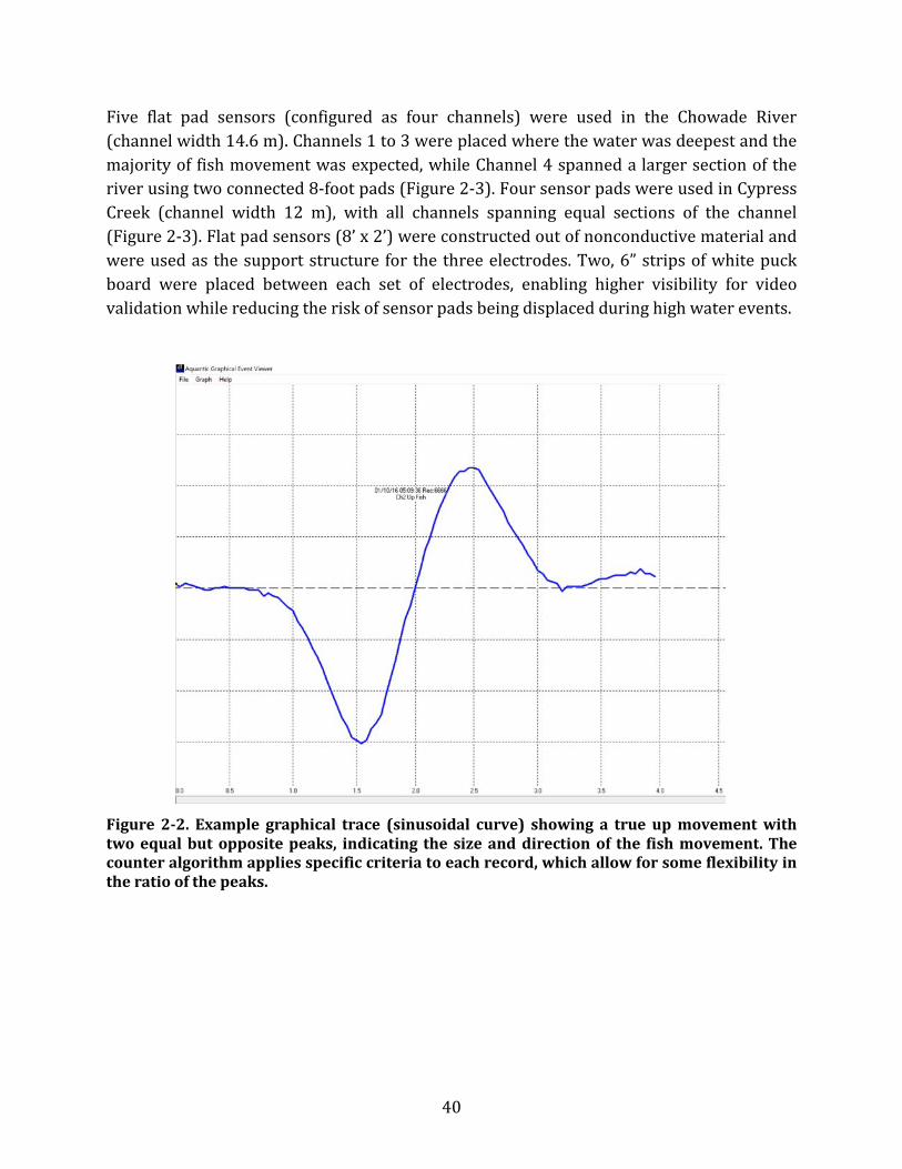
Five flat pad sensors (configured as four channels) were used in the Chowade River (channel width 14.6 m). Channels 1 to 3 were placed where the water was deepest and the majority of fish movement was expected, while Channel 4 spanned a larger section of the river using two connected 8-foot pads (Figure 2-3). Four sensor pads were used in Cypress Creek (channel width 12 m), with all channels spanning equal sections of the channel (Figure 2-3). Flat pad sensors (8’ x 2’) were constructed out of nonconductive material and were used as the support structure for the three electrodes. Two, 6” strips of white puck board were placed between each set of electrodes, enabling higher visibility for video validation while reducing the risk of sensor pads being displaced during high water events.

Figure 2-2. Example graphical trace (sinusoidal curve) showing a true up movement with two equal but opposite peaks, indicating the size and direction of the fish movement. The counter algorithm applies specific criteria to each record, which allow for some flexibility in the ratio of the peaks.

40

Figure 2-3. Configuration of the resistivity counter sensor pads, power system and video validation system in the Chowade River and Cypress Creek, 2018.

Counter Validation We continuously operated a video monitoring system at each counter site to validate the resistivity counter data. In the Chowade River, five video cameras were used to monitor the counter pads, while four were used in Cypress Creek. The cameras were placed directly above the sensor pads on a cableway system (Figure 2-3) and centered to capture the full span of the pad. Background LED lights were installed beside the cameras for nighttime recording. All cameras recorded video in five-minute segments and video data were stored in dedicated hard drives within a custom-built desktop computer operated at each site.

Raw counter data (i.e., graphical traces of up movements, down movements, and unclassified events) were validated using video data to determine the number of true positives, false positives, false negatives, and counter accuracy (Table 2-2). We used a multi-step validation process that included targeted validation of counter up and down counts, and random validation of additional video data (see validation process detailed in Figure 2-4). In the rare event that video data were unavailable to validate a counter event (e.g., due to power outages, high turbidity, or camera issues), the counter record in question was included in the final count but could not be included in the accuracy estimate.

During targeted validation, each graphical trace (up or down) was verified by watching the corresponding video data and one minute before and after. The two-minute time bracket accounted for minor time-stamp discrepancies between the counter and the video and

41

allowed the analyst to verify movement records and determine fish species. Eighteen hours of targeted footage were reviewed for the Chowade River, and eight hours were reviewed for Cypress Creek. The disparity of effort between sites was due to the higher number of counter records in the Chowade River relative to Cypress Creek.

We also reviewed a subset of randomly-selected video segments to determine the number of false negatives (i.e., a fish was observed on the video but the counter recorded no trace). For each full day of video, 22 randomly-selected 10-minute segments of video were reviewed. The amount of video watched was based on estimated population size, number of fish expected to be validated, total number of hours available to be validated, and time constraints (Braun et al. 2016). Approximately 16% of the total video record was analyzed at each site, corresponding to 168 hours for the Chowade River and 233 hours for Cypress Creek. The total number of false negatives was determined by expanding the validated count (targeted and random validation combined) to the total hours of video data collected.

The numbers of true positives (TP), false positives (FP), and false negatives (FN) were used to calculate counter accuracy (A), summarized by direction (up and down), species (Bull Trout, Mountain Whitefish, etc.), and counter channel:

(2.1) 𝐴𝐴 =𝑇𝑇𝑇𝑇

𝑇𝑇𝑇𝑇 + 𝐹𝐹𝑇𝑇 + 𝐹𝐹𝑁𝑁

Accuracies were used to assess the performance of the counter, and to adjust the counter estimate to obtain final estimates of abundance.

Table 2-2. Definition of error rates used to classify counter records during validation.

Error Category Resistivity Counter Video Review

True Positive Graphical trace (up or down)

Fish observed and movement agrees with up or down classification

False Positive Graphical trace (up or down) No fish movement occurred

False Negative No graphical trace Fish movement occurred

Unclassified Graphical trace (up or down) Video data not available

42

Length Measurements and Species Determination We measured the length of each fish observed during video validation to aid with species determination and to develop a site-specific length vs PSS relationship. The true length of a fish measured on the video was determined using the ratio of the on-screen pad length and on-screen fish length:

(2.2) 𝐹𝐹𝜋𝜋𝑇𝑇 =𝐹𝐹𝜋𝜋𝑚𝑚𝑇𝑇𝜋𝜋𝑚𝑚

𝑒𝑒 𝑇𝑇𝜋𝜋𝑇𝑇

where FLT is the estimated true fish length (standard length), FLm is the fish length as measured on the video screen, PLm is the distance between electrodes at the point where the fish crossed as measured on the video screen, and PLT is the true distance between the upper and lower electrodes on the counter pad (60 cm).

During video validation, fish were identified to species (Bull Trout, Mountain Whitefish, or Rainbow Trout) based on length (R.L. & L. Environmental Services Ltd. 1995), colouration, and body shape. In the unlikely event that the species could not be identified or agreed upon by two independent analysts (e.g., during low visibility conditions), we categorized the record as unknown.

43

Figure 2-4. Counter validation protocol.

Raw Counter Measurement

- Counter measures a change in resistance as fish passes over the counter site - Each trace is examined by a reviewer and classified as an up, down, or event

Up

Fish is moving upstream, passing over all three electrodes

Down

Fish is moving downstream, passing over all three electrodes

Event

Partial or incomplete movement of fish over the counter electrodes (in any direction) caused by a fish nosing up, falling back, or sitting on electrodes. Events may also be caused by air entrainment or debris flow over the electrodes.

Targeted Video Validation

Random Video Validation

- All up and down records are reviewed on video

- Reviewer watches record plus 1 minute before and after record

- Record is classified as either: - True positive - False positive

- Subset of randomly-selected video segments is reviewed

- For each 24-hour period, 20 randomly selected 10-minute segments are reviewed

- Fish movement observed on video but without paired graphical trace are classified as false negative

Calculate Error Rates and Accuracy

- Determine the total number of true positives (TP), false positives (FP), and false negatives (FN), summarized by:

- Movement direction (up and down) - Species (Bull Trout, Mountain Whitefish, etc) - Counter channel

- Calculate accuracy (A) for each category

44

Migration Timing We observed three unique movement behaviours during the Bull Trout spawning migration:

1. Up-migration: Moving upstream to spawn; 2. ‘Recycling’: Movement back and forth across the counter site; and 3. Kelting: Moving downstream after spawning completion.

Timing of these three movement behaviours overlap, and the approximate date of the kelting onset must be determined prior to estimating abundances for up-migrating and kelting Bull Trout.

The onset of the kelt out-migration in the Halfway Watershed typically begins in late August or early September (R.L. & L. Environmental Services Ltd. 1995). Prior to the kelting onset, downstream movements were considered recycling and these down counts were subtracted from up counts. Recycling and kelting can be distinguished because the number of recycling events generally mirrors that of daily up-counts, while kelting generally follows a normal distribution. Exact kelting dates can be determined for PIT-tagged fish that are detected during both their upstream and downstream migrations, but to determine an average kelting date this method requires a large sample of PIT-tagged fish.

Kelting onset and peak kelting dates can also be estimated by fitting a normal probability density function to downstream migration data. We fit a normal probability density function to daily down counts from September 1 to October 2 by minimizing the sum of squares of the predicted and observed count data. We selected these dates to isolate the potential kelting period based on the findings of previous monitoring in the Halfway Watershed (R.L. & L. Environmental Services Ltd. 1995). We estimated the mean, standard deviation and a scale parameter for the normal distribution. The fitted mean represented the peak date of the kelt migration while the scale parameter provided an estimate of kelting abundance (which can also be compared to the resistivity counter kelting abundance). We defined the date of kelting onset as the date when 5% of the kelts had migrated according to the daily kelt abundances predicted by the normal model.

Abundance Estimates Bull Trout abundance estimates were generated for kelting migrations past the counter site. In 2018, the upstream abundance estimate captured only a portion of the run (i.e., migration began prior to counter installation), while the kelting abundance encompassed the entire kelting period. The estimated abundance for the upstream migration was calculated using:

45

(2.3) 𝐸𝐸𝑈𝑈 = ��Ut

Au−𝐷𝐷𝑡𝑡A𝑑𝑑�

𝑘𝑘

𝑡𝑡=1

+ �Ut

Au

𝑛𝑛

𝑡𝑡=𝑘𝑘

where EU is the up-migration abundance estimate, 𝑅𝑅𝑡𝑡 is the total number of counter upstream counts, 𝐷𝐷𝑡𝑡 is the corresponding number of downstream counts, 𝐴𝐴𝑢𝑢 is the upstream counter accuracy, 𝐴𝐴𝑑𝑑 is the downstream counter accuracy, 𝑘𝑘 is the date of kelting onset, and 𝑛𝑛 is the date of the latest confirmed Bull Trout up-count. The estimated abundance for the kelting migration was calculated using:

(2.4) 𝐸𝐸𝑘𝑘 = �Dk

Ad

𝑗𝑗

𝑡𝑡=𝑘𝑘

where Ek is the down-migration abundance estimate, Dk is the number of downstream counts, Ad is the downstream counter accuracy, k is the date of kelting onset and j is the date of the last confirmed Bull Trout down-count.

2.2.5 PIT Telemetry Operations

Antenna Design, Power and Operations PIT arrays were operated in the Chowade River and Cypress Creek in 2018 to detect fish tagged under Mon-1b, Task 2c (Site C Reservoir Tributaries Fish Population Indexing Survey) and Mon-2, Task 2a (Peace River Large Fish Indexing Survey). Four rigid framed pass-over antennas were designed and built to create two-antenna arrays at each site. Antennas were 13.5 × 1.25 m in the Chowade River and 10.5 × 1.25 m at Cypress Creek and were constructed out of 1.5” ABS pipe with cross braces every 1.5 m to maintain a rigid frame (Figure 2-5A). Antennas were designed to lie flat on the streambed and were anchored with Duckbill earth anchors and sandbags so that fish would have to swim over the antennas to be detected (Figure 2-5B). Each antenna was connected to a remote tuner box (Oregon RFID, Portland, OR) and a single reader (Oregon RFID) via twin-axial cable. We manually tuned and tested antennas to ensure optimal read range and tag reading performance.

Each antennas were powered by an independent battery bank maintained by solar panels (Table 2-1). To remedy the electrical interference that reduced the read range of the antennas in 2017, we deployed a passive line noise filter (recently developed by Oregon RFID) that removed noise on the powerline from the solar charge controller. The reduced electrical interference allowed us to run two antennas concurrently at both sites. In the Chowade River, two antennas were operational throughout the resistivity counter

46

monitoring period (August 16 to October 1). In Cypress Creek, because of the increased read range of the antennas, the original antenna configuration (one antenna upstream and one downstream of the counter) caused interference with the resistivity counter and we moved the upstream antenna to a new downstream site (Figure 2-3). We operated one antenna in Cypress Creek prior to the antenna re-configuration on August 29, and two antennas from August 29 to October 2.

Data were downloaded from PIT readers during each weekly site visit and safely stored on an on-site computer. We collated raw PIT files using the PITR package for R (Harding et al. 2018) developed by InStream Fisheries Research. Detection efficiency, or the percentage of tags detected by both antennas in the array, was calculated using PITR during the time periods in which two antennas were running at each site.

Figure 2-5. PIT antenna design (A) and deployment (B) at Cypress Creek, 2018.

Read Range Surveys We conducted detailed read range testing of the antennas during each site visit to develop an understanding of the read range of the PIT arrays during the monitoring period. During a survey, we measured the following parameters (in meters) at each cross brace of the frame (every 1.5 m) along the length of the antenna:

(1) Water depth: distance from streambed to water surface; (2) Antenna depth: distance from top of antenna to water surface; and (3) Detection range of 12, 23 and 32 mm PIT tags: distance from the antenna to

the depth at which the antenna could no longer detect the test tag.

47

We used the read range testing to determine the proportion of the water column that was readable for the three sizes of PIT tags deployed under other FAHMFP monitoring programs. Summarizing these data across all surveys yielded an estimate of the total proportion of the water column that was readable.

Movement Ecology

We summarized the movement of fish detected on the Chowade River and Cypress Creek PIT arrays to identify critical periods of upstream and downstream migrations, and patterns in diel movement. The use of two antennas made it possible to determine movement direction for any fish detected by both antennas. Movement summaries helped corroborate data collected by the resistivity counter and aided with estimating the onset of kelt-migration. Tagging and sampling information for PIT-tagged fish was obtained from Golder Associates Ltd. (Dustin Ford).

2.3 Results 2.3.1 Chowade River

Environmental Conditions

Halfway River discharge (log-transformed) was strongly correlated with water depths measured at the Chowade River counter site (r = 0.96; p < 0.001; Figure 2-26A). Average stage height at the counter site between August 10 and October 1 was 0.41 m (range: 0.30-0.55 m). High discharge after a local rainstorm in late July prevented the installation of in-river equipment until August 16, when Halfway River discharge was 28 m3s-1 and stage height at site was 0.49 m (Figure 2-6). In contrast, in 2016 the counter was installed on July 26 when Halfway River discharge was 50 m3s-1 . The change in installation depth may be related to the placement of the sensors (i.e., their location in river) or high-discharge events in the winter of 2016-2017 that resulted in changes to the channel morphology at the counter site. Establishing a more permanent hydrological station at each site may improve the relationship between Halfway River discharge and stage height. A Halfway River discharge of 28 m3s-1 will be the installation limit in future years.

48

Figure 2-6. (A) Daily means of Halfway River discharge (black line) and Chowade River water depth (red line). Dashed line represents water level when instream equipment was installed. (B) The relationship between the Halfway River discharge (Station 07FA003) and water depth at the Chowade River counter site from August 10 to October 2, 2018.

Resistivity Counter Counter Validation

Fish observed during video validation were categorized as Bull Trout (≥40 cm; Figure 2-7A), Mountain Whitefish (Figure 2-7B), Rainbow Trout, or unknown (Figure 2-7C). The unknown category included small bodied fish (<40 cm) such as Bull Trout, Rainbow Trout, Mountain Whitefish, and Arctic Grayling that were too small to identify, and adult fish that

49

could not be accurately identified using the video footage. In 2018, only 4 of 719 large-bodied fish could not be identified during Chowade River video validation.

We estimated total length for all fish observed during video validation (Table 2-3). We modelled the species-specific relationship between length and PSS (as measured by the counter) for Bull Trout and Mountain Whitefish to determine if PSS could be used to identify species for each counter record (we did not have sufficient Rainbow Trout data to model length vs PSS). As in 2017, we did not find a positive relationship between length and PSS (Figure 2-8) and we used video validation to determine species for each counter record.

We estimated channel-specific and direction-specific counter accuracy using video validation of counter records. Up-accuracy across all channels was 91%, and down-accuracy was 50%, suggesting the counter underestimated the number of Bull Trout moving upstream and downstream over the counter. Up-accuracies in Channels 1 and 2 were >88%, and these were the channels most actively used by Bull Trout (72% of upstream movements; Table 2-4; Figure 2-9). Up-accuracies in Channels 2 and 4 were 100%, but these channels were less frequently used for upstream movements. Down-accuracies were ~50% across all channels, and downstream movements were more evenly distributed across all four channels (Figure 2-9). We expected down-accuracy to be lower than up-accuracy because Bull Trout travel lower in the water column while moving upstream, and are therefore closer to the counter sensors.

We also determined counter accuracy for Mountain Whitefish. As expected due to their schooling behaviour and small size, the accuracy for Mountain Whitefish was substantially lower than for Bull Trout, with up- and down-accuracies of 12% and 4% (both underestimating), respectively.

50

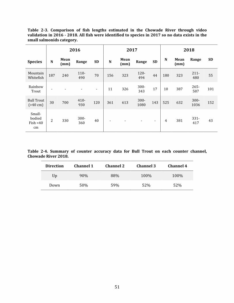
Table 2-3. Comparison of fish lengths estimated in the Chowade River through video validation in 2016 - 2018. All fish were identified to species in 2017 so no data exists in the small salmonids category.

2016 2017 2018

Species N Mean (mm) Range SD N Mean

(mm) Range SD N Mean (mm)

Range SD

Mountain Whitefish 187 240 110-

490 70 156 323 120-494 44 180 323 211-

480 55

Rainbow Trout - - - - 11 326 300-

343 17 10 387 265-587 101

Bull Trout (>40 cm) 30 700 410-

930 120 361 613 300-1080 143 525 632 300-

1036 152

Small- bodied

Fish <40 cm

2 330 300-360 40 - - - - 4 381 331-

417 43

Table 2-4. Summary of counter accuracy data for Bull Trout on each counter channel, Chowade River 2018.

Direction Channel 1 Channel 2 Channel 3 Channel 4

Up 90% 88% 100% 100%

Down 50% 59% 52% 52%

51

Figure 2-7. Example of species identification from video footage: (A) large-bodied Bull Trout, (B) small school of Mountain Whitefish, and (C) species unknown.

52

Figure 2-8. Peak signal size relative to standard length (mm) of Bull Trout (blue) and Mountain Whitefish (grey) observed moving upstream during video validation on each counter channel, 2018.

53

Figure 2-9. Distribution of confirmed Bull Trout (blue) and Mountain Whitefish (grey) among channels, separated by upstream (top panel) and downstream (bottom panel) movements, Chowade River 2018.

Migration Timing

The normal density function estimated that the Bull Trout kelt out-migration began on September 9 (Figure 2-10) and peaked on September 17 (SD 6.5 days). Most Bull Trout and Mountain Whitefish moved upstream during low-light conditions; 507 individual Bull Trout and 165 Mountain Whitefish schools moved after civil twilight while 18 Bull Trout and 15 Mountain Whitefish schools moved during the day (Figure 2-11).

54

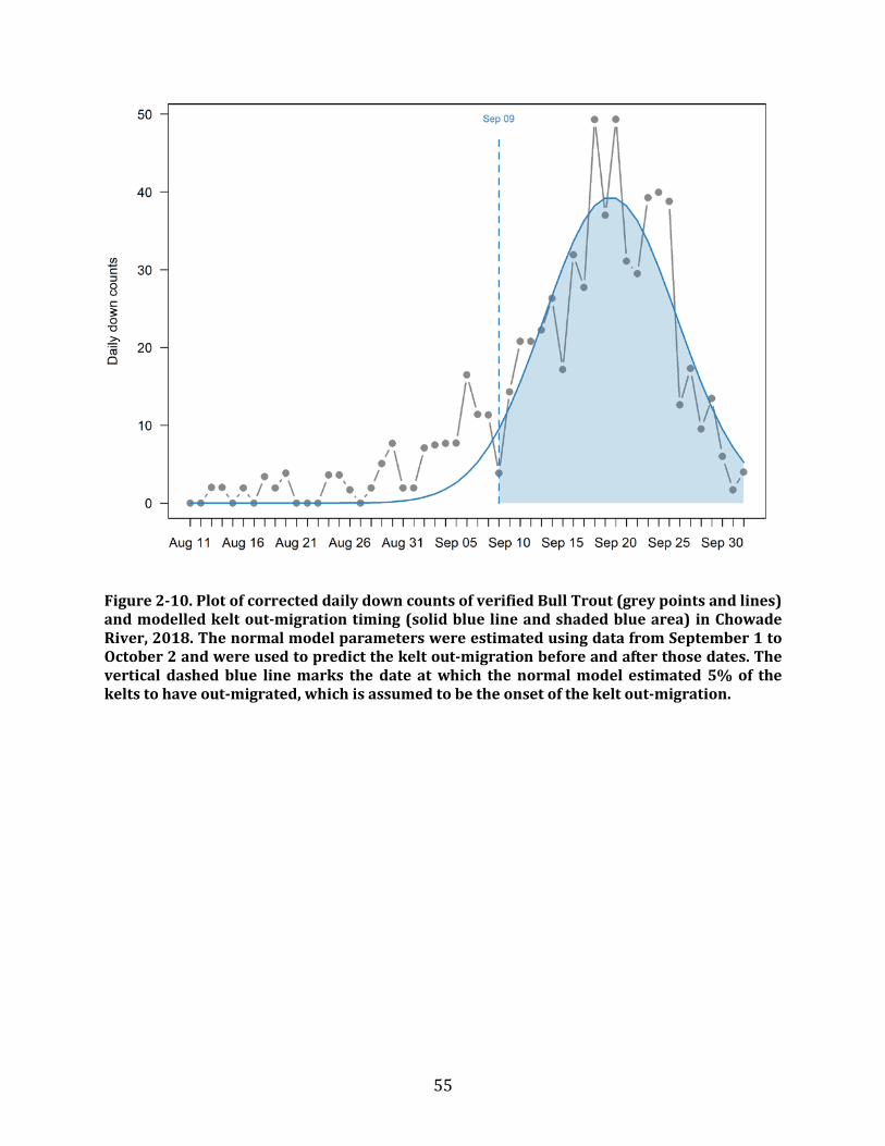
Figure 2-10. Plot of corrected daily down counts of verified Bull Trout (grey points and lines) and modelled kelt out-migration timing (solid blue line and shaded blue area) in Chowade River, 2018. The normal model parameters were estimated using data from September 1 to October 2 and were used to predict the kelt out-migration before and after those dates. The vertical dashed blue line marks the date at which the normal model estimated 5% of the kelts to have out-migrated, which is assumed to be the onset of the kelt out-migration.

55

Figure 2-11. Number of Bull Trout (blue) and Mountain Whitefish (dark grey) observed from video during each hour (relative to civil twilight) over the counter pads in Chowade River from August 11 to October 2, 2018.

Abundance Estimate

After accounting for counter accuracy and the date of kelting onset (Equation 2.4), the kelt abundance for the Chowade River was 564 Bull Trout. We could not generate an upstream abundance due to the late counter installation; however, the counter detected 147 Bull Trout moving upstream past the counter between August 11 and October 2 (Figure 2-12). Subsequent to counter installation the counter detected a decline in up-counts and corresponding increase in down-counts, which further indicated (in agreement with the normal density model) that the counter captured the entire kelting migration period of September 9 to October 2.

56

Figure 2-12. (A) Water depth (m) plotted to assess whether specific water levels corresponded with specific fish movements. (B) Bull Trout daily up (blue) and down (black) counts, and (C) cumulative net up counts (blue line) from August 11 to October 2 and cumulative down counts of kelts (black line) from September 9 to October 2 in the Chowade River 2018.

57

PIT Telemetry Detection Effeciency

Read ranges of the 23 and 32 mm PIT tags met or exceeded the water depth along the length of the two antennas in the Chowade River (Figure 2-13, Figure 2-14). The proportion of the water column within which 23 and 32 mm PIT tags could be detected was 100% across all seven surveys. Read ranges of the 12 mm PIT tags were ~60% of the water depth at the thalweg, but overall the proportion of the water column within which 12 mm PIT tags could be detected was >76% for both antennas (Figure 2-15, Figure 2-16). Read ranges were more consistent for all tag types in 2018 (SD = 0.09) when compared to 2017 (SD = 0.31).

We detected 36 fish on the Chowade River PIT array (24 Bull Trout, 12 Rainbow Trout) with 12, 23 and 32 mm PIT tags. Detection efficiency (for all species) was 94% for the PIT array in the Chowade River (35 of 36 tags detected by both antennas) (Table 2-5).

58

Figure 2-13. Read range of 12 mm (red), 23 mm (blue) and 32 mm (green) PIT tags across the seven weekly surveys of the Chowade River upstream PIT antenna. Shaded blue area represents water level.

59

Figure 2-14. Read range of 12 mm (red), 23 mm (blue) and 32 mm (green) PIT tags across the seven weekly surveys of the Chowade River downstream PIT antenna. Shaded blue area represents water level.

60

Figure 2-15. Proportion of the water column (mean ± SD) in the Chowade River that could effectively read all PIT tags (12, 23, and 32 mm) at the upstream PIT antenna (top panel). Because read range for 23 and 32 mm tags was 100% of the water column for all surveys, only data from 12 mm tags is shown (red points), with the orange shaded area illustrating the portion of the river channel where 100% of PIT tags of all sizes could be read. The bottom panel depicts the river channel profile at the Chowade River counter site in 2018.

61

Figure 2-16. Proportion of the water column (mean ± SD) in the Chowade River that could effectively read all PIT tags (12, 23, and 32 mm) at the downstream PIT antenna (top panel). Because read range for 23 and 32 mm tags was 100% of the water column for all surveys, only data from 12 mm tags is shown (red points), with the orange shaded area illustrating the portion of the river channel where 100% of PIT tags of all sizes could be read. The bottom panel depicts the river channel profile at the Chowade River counter site in 2018.

62

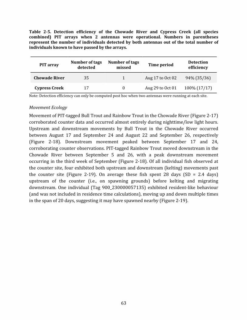
Table 2-5. Detection efficiency of the Chowade River and Cypress Creek (all species combined) PIT arrays when 2 antennas were operational. Numbers in parentheses represent the number of individuals detected by both antennas out of the total number of individuals known to have passed by the arrays.

PIT array Number of tags detected

Number of tags missed Time period Detection

efficiency

Chowade River 35 1 Aug 17 to Oct 02 94% (35/36)

Cypress Creek 17 0 Aug 29 to Oct 01 100% (17/17)

Note: Detection efficiency can only be computed post hoc when two antennas were running at each site.

Movement Ecology

Movement of PIT-tagged Bull Trout and Rainbow Trout in the Chowade River (Figure 2-17) corroborated counter data and occurred almost entirely during nighttime/low light hours. Upstream and downstream movements by Bull Trout in the Chowade River occurred between August 17 and September 24 and August 22 and September 26, respectively (Figure 2-18). Downstream movement peaked between September 17 and 24, corroborating counter observations. PIT-tagged Rainbow Trout moved downstream in the Chowade River between September 5 and 26, with a peak downstream movement occurring in the third week of September (Figure 2-18). Of all individual fish observed at the counter site, four exhibited both upstream and downstream (kelting) movements past the counter site (Figure 2-19). On average these fish spent 28 days (SD = 2.4 days) upstream of the counter (i.e., on spawning grounds) before kelting and migrating downstream. One individual (Tag 900_230000057135) exhibited resident-like behaviour (and was not included in residence time calculations), moving up and down multiple times in the span of 20 days, suggesting it may have spawned nearby (Figure 2-19).

63

Figure 2-17. Number of Bull Trout (blue) and Rainbow Trout (grey) detected on the Chowade River PIT array during each hour from August 17 to October 1, 2018.

64

Figure 2-18. Upstream (blue) and downstream (grey) movements by PIT-tagged Bull Trout (top panel) and Rainbow Trout (bottom panel) on the Chowade River PIT array 2018.

65

Figure 2-19. Migration behavior of individual Bull Trout observed at the Chowade River counter site in 2018. These five individuals exhibited kelting behavior. Red star indicates the date the PIT antennas were installed and assumed upstream movement.

66

2.3.2 Cypress Creek Environmental Conditions

There was a strong log-linear relationship between Halfway River discharge and water depth at the Cypress Creek counter site (r = 0.97, p < 0.001; Figure 2-20). Average stage height at the counter site between August 1 and October 1 was 0.13 m (range: 0.0-0.39 m). A rain event in late July prevented the installation of in-river equipment in Cypress Creek until August 9 when Halfway River discharge was 41.5 m3s-1 and stage height at site was 0.30 m (Figure 2-20B). A Halfway discharge of 41.5 m3s-1 will be the installation limit in future years.

Figure 2-20. A) Daily means of Halfway River discharge (black line) and Cypress Creek water depth (red line). Dashed line represents the water level at site when the in-river equipment was installed (installation limit). B) The relationship between the Halfway River discharge (Station 07FA003) and water depth at the Cypress River counter site from August 1 to October 1, 2018.

67

Resistivity Counter Counter Validation

The two most abundant species observed in Cypress Creek were Bull Trout (n = 230) and Mountain Whitefish (>20 schools; Table 2-6). Three Rainbow Trout were identified, and Arctic Grayling may have also been present. Overall, we did not find a positive relationship between standard length and PSS (Figure 2-21), so we used video validation to determine species for each counter record.

We estimated channel-specific and movement-specific counter accuracy using video validation of counter records. The Cypress Creek resistivity counter underestimated the number of Bull Trout moving over the counter with an up-accuracy of 85% and a down-accuracy of 28% (Table 2.8). Up-accuracies in Channels 2 and 3 were 72% and 100%, respectively, and these were the channels most actively used by Bull Trout (85% of upstream movements; Table 2-7; Figure 2-22). Up-accuracy was 100% in Channel 1 (with 4% of upstream movements) and 71% in Channel 4 (11% of upstream movements). Channels 2 and 3 accounted for the majority of downstream movements (89%), with accuracies of 26% and 29%, respectively.

We also determined counter accuracy for Mountain Whitefish. The down-accuracy for Mountain Whitefish was 2%, and no upstream Mountain Whitefish movements were observed.

Table 2-6. Comparison of fish lengths estimated in Cypress Creek through video validation in 2018. Note that the small salmonids were difficult to identify but also difficult to measure.

2017 2018

Species N Mean (mm) Range SD N Mean

(mm) Range SD

Mountain Whitefish 207 259 83-463 70 20 323 243-380 32

Rainbow Trout 9 308 171-400 73 3 354 292-

450 84

Bull Trout (>40 cm) 76 556 308-844 133 230 496 279-

900 97

Small-bodied Fish < 40 cm 3 - - - 14 332 216-

575 90

68

Table 2-7. Summary of counter accuracy data for Bull Trout on each counter channel, Cypress Creek 2017.

Direction Channel 1 Channel 2 Channel 3 Channel 4

Up 100 72% 100% 71%

Down 19% 26% 29% 100%

Figure 2-21. Peak signal size relationship to standard length (mm) of Bull Trout observed moving upstream during video validation on each counter channel at Cypress Creek 2018.

69

Figure 2-22. Distribution of confirmed Bull Trout (blue) and Mountain Whitefish (grey) among channels, separated by upstream (top panel) and downstream (bottom panel) movements in Cypress Creek 2018.

Migration Timing

The normal density function estimated that the Cypress Creek kelt out-migration began on September 11 (Figure 2-23) and peaked on September 15 (SD 3.3 days). As in the Chowade River, most upstream movement occurred during low light/night hours (~200 individuals), with only 28 individuals detected moving during daylight hours (Figure 2-24). Mountain Whitefish showed a similar pattern with one school moving during the day and 19 schools moving at night.

70

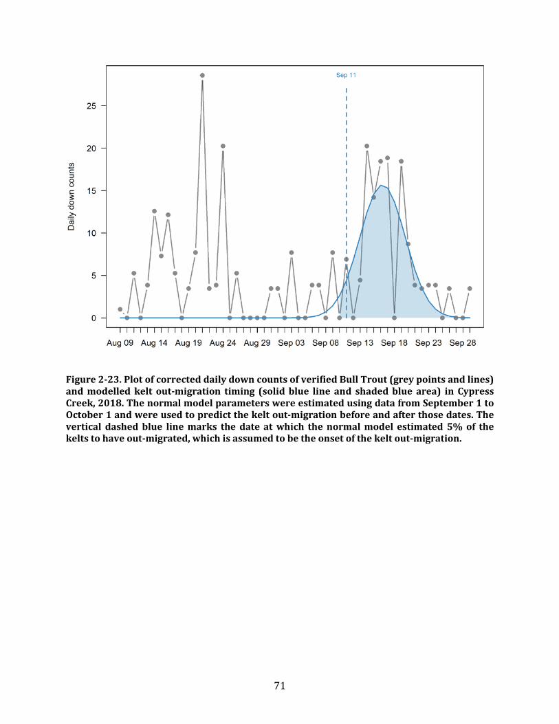
Figure 2-23. Plot of corrected daily down counts of verified Bull Trout (grey points and lines) and modelled kelt out-migration timing (solid blue line and shaded blue area) in Cypress Creek, 2018. The normal model parameters were estimated using data from September 1 to October 1 and were used to predict the kelt out-migration before and after those dates. The vertical dashed blue line marks the date at which the normal model estimated 5% of the kelts to have out-migrated, which is assumed to be the onset of the kelt out-migration.

71

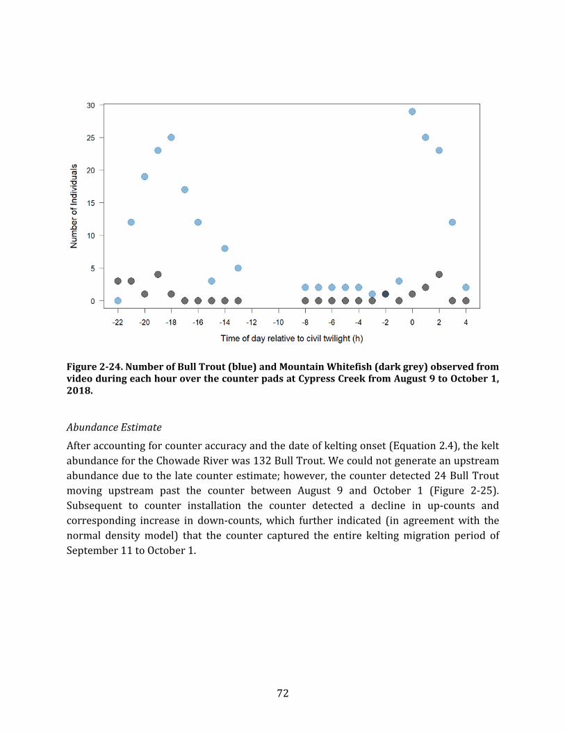
Figure 2-24. Number of Bull Trout (blue) and Mountain Whitefish (dark grey) observed from video during each hour over the counter pads at Cypress Creek from August 9 to October 1, 2018.

Abundance Estimate

After accounting for counter accuracy and the date of kelting onset (Equation 2.4), the kelt abundance for the Chowade River was 132 Bull Trout. We could not generate an upstream abundance due to the late counter estimate; however, the counter detected 24 Bull Trout moving upstream past the counter between August 9 and October 1 (Figure 2-25). Subsequent to counter installation the counter detected a decline in up-counts and corresponding increase in down-counts, which further indicated (in agreement with the normal density model) that the counter captured the entire kelting migration period of September 11 to October 1.

72

Figure 2-25. A) Water depth (m), plotted to assess whether specific water levels correspond with specific fish movements, B) Bull Trout daily up (blue) and down (black) counts, and C) the cumulative net up counts (blue line) from August 9 to September 29, and cumulative down counts of kelts (black line) from September 11 to October 1 in Cypress Creek 2018.

73

PIT Telemetry Detection Efficiency

Read ranges of the 23 and 32 mm PIT tags met or exceeded the water depth along the length of the antennas in Cypress Creek (Figure 2-26, Figure 2-27, Figure 2-28, Figure 2-29). The proportion of the water column within which 23 and 32 mm PIT tags were detectable was 100% across all five surveys. Read ranges of the 12 mm PIT tags were 75% (upstream antenna) and 80% (downstream antenna) at the thalweg, but overall the proportion of the water column within which 12 mm PIT tags could be detected was >79% at both antennas. Read ranges were less variable in 2018 (SD = 0.16) for 12 mm tags when compared to 2017 results (SD = 0.32).

From August 11 to 29, four Bull Trout and two unidentified PIT tags were detected by a single antenna operated in Cypress Creek (direction of movement and detection efficiency could not be determined during this period). From August 29 to October 1 two antennas were operational and the PIT array detected 14 Bull Trout and three Rainbow Trout with 12, 23 and 32 mm PIT tags. While two antennas were operational, detection efficiency was 100% for the PIT arrays in Cypress Creek (17 of 17 tags detected by both antennas; Table 2-5).

74

Figure 2-26. Read range of 12 mm (red), 23 mm (blue), and 32 mm (green) PIT tags across the five weekly surveys of the Cypress Creek upstream PIT antenna in 2018.

75

Figure 2-27. Read range of 12 mm (red), 23 mm (blue), and 32 mm (green) PIT tags across the five weekly surveys of the Cypress Creek downstream PIT antenna in 2018.

76

Figure 2-28. Proportion of the water column (mean ± SD) in Cypress Creek that could effectively read all PIT tags (12, 23, and 32 mm) at the downstream PIT antenna (top panel). Because read range for 23 and 32 mm tags was 100% of the water column for all surveys, only data from 12 mm is shown (red points), with the orange shaded area illustrating the portion of the river channel where 100% of PIT tags of all sizes could be read. The bottom panel depicts the river channel profile at the Cypress Creek counter site in 2018.

77

Figure 2-29. Proportion of the water column (mean ± SD) in Cypress Creek that could effectively read all PIT tags (12, 23, and 32 mm) at the upstream PIT antenna (top panel). Because read range for 23 and 32 mm tags was 100% of the water column for all surveys, only data from 12 mm is shown (red points), with the orange shaded area illustrating the portion of the river channel where 100% of PIT tags of all sizes could be read. The bottom panel depicts the river channel profile at the Cypress Creek counter site in 2018.

Movement Ecology

PIT-tagged Bull Trout and Rainbow Trout in Cypress Creek moved almost entirely after dark (Figure 2-30), consistent with resistivity counter results. Downstream movements of PIT-tagged Bull Trout occurred between September 7 and October 2 (Figure 2-31) and peaked in the third week of September (September 19 to 23). Although movement behaviour and direction were difficult to confirm at Cypress Creek in early August (because only one antenna was operational), we were able to infer kelting behaviour for three fish (Figure 2-32) that had residence times of 20, 26 and 31 days upstream of the counter (mean = 25.7, SD = 5.5).

78

Figure 2-30. Number of Bull Trout (blue) and Rainbow Trout (grey) detected on the Cypress Creek PIT array during each hour from August 9 to October 1, 2018.

79

Figure 2-31. Downstream (grey) and upstream movements (blue) by PIT tagged Bull Trout (top panel) and Rainbow Trout (bottom panel) on the Cypress Creek PIT array. No upstream movements of Bull Trout were observed in 2018.

80

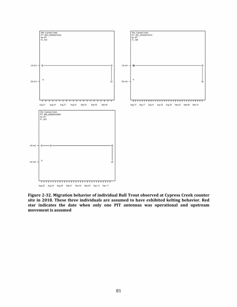
Figure 2-32. Migration behavior of individual Bull Trout observed at Cypress Creek counter site in 2018. These three individuals are assumed to have exhibited kelting behavior. Red star indicates the date when only one PIT antennas was operational and upstream movement is assumed

*

*

*

81

2.4 Discussion 2.4.1 Resistivity Counter Operation

We enumerated Bull Trout in the Chowade River and Cypress Creek using resistivity counters and PIT arrays. We monitored the full kelting outmigration in both tributaries and estimated that 564 and 132 Bull Trout kelts migrated downstream past the counter sites in the Chowade River (between September 9 and October 2) and Cypress Creek (between September 11 and October 1), respectively. Downstream counter accuracy was moderate in both tributaries (50% in the Chowade River and 28% in Cypress Creek); however, our confidence in the kelting estimates is high due to the extensive targeted and random counter validation that was performed for both datasets.

Due to high water levels in July we were unable to install the resistivity counters in time to fully monitor upstream migrations, but we can use the kelt estimates as indices of spawner abundance. Kelt estimates have successfully been used as a proxy for Bull Trout spawner abundance in other streams in British Columbia, and should provide a reasonable measure of spawner abundance (Andrusak 2009). Kelt estimates do not account for resident fish (i.e., those that do not move downstream) or fish that die after spawning, and it is therefore important to understand the annual kelting proportion for a population. Although we may not be able to monitor the full upstream spawning migration in Cypress Creek and the Chowade River, we may be able to capture the peak and tail end of the migration in years when mid-July flow are amenable to equipment installation. Assuming the upstream migration follows a normal distribution, the peak count and migration tail could be used to estimate the full spawner abundance and spawner to kelt ratio.

Individual tagging data (i.e., PIT and radio tagging) can also be used to determine the kelting ratio for a spawning population. Given sufficient PIT-tagged fish, a kelting estimate could be determined for the PIT-tagged subset and applied to the full population. For example, if 20 PIT-tagged Bull Trout moved upstream past the counter site but only 15 were detected making kelting migrations, the kelting ratio would be estimated as 75%. Radio telemetry can also be used to determine migration timing and movement behaviour for a small subset of tagged fish. Radio telemetry can inform kelting proportions and also provide insight into whether Bull Trout move between tributaries within or between years.

Understanding both natural variability in abundance and process error in obtaining estimates is critical to detecting changes in abundance throughout the monitoring period. Consequently, rigorous methodology is in place to quantify the accuracy of counter estimates. Modifications to counter settings improved upstream counter accuracy in both the Chowade River and Cypress Creek. Accuracy improved from 69% (2017) to 91% (2018) in the Chowade River and from 55% (2017) to 85% (2018) in Cypress Creek. Upstream counter accuracies in 2018 were similar to or higher than accuracies observed in other systems in British Columbia (Ramos-Espinoza et al. 2011, Burnett et al. 2017). For

82

example, flat pad counter sensors used to enumerate Coho Salmon (O. kisutch) in the Lower Bridge River had up-accuracies of 70% (Burnett et al. 2017). In the Chilcotin River, flat pad sensors monitoring Chinook Salmon had upstream accuracies >80% and downstream accuracies >53% (Ramos-Espinoza et. al. 2011).

Down-count accuracies in 2018 were low for both the Chowade River and Cypress Creek (50% and 28%, respectively). Under optimal conditions, we would expect down accuracies to be between 60 and 70% (e.g., Ramos-Espinoza et al. 2011). The low accuracies in the Chowade River and Cypress Creek are likely a result of fish behaviour and site morphology. Bull Trout generally move faster and travel higher in the water column when migrating downstream in the direction of flow, making it more difficult for the counter to detect their movement. The Cypress Creek counter is located in a fast-moving riffle, and the Chowade River counter is located in an area with a relatively deep thalwag, both of which likely affected respective counter accuracy. Improving downstream counter accuracy is important for accurately determining kelting abundance, and we will continuously work to improve accuracy through counter pad innovation and testing.

2.4.2 Bull Trout Spawner Size

Size distributions estimated through video validation were consistent between 2017 and 2018 for the Chowade River and Cypress Creek (Ramos-Espinoza et al. 2018). Average total length estimated from the Chowade River video data (632 mm, range 300-1036 mm) were similar to average fork lengths obtained during Bull Trout angling in 1995 and 1996 (Baxter 1997; females 609.75 mm, males 630.02 mm), and measured at a fish fence operated in the Chowade River in 1994 (R.L. & L. Environmental Services Ltd. 1995; 604 mm). Total lengths measured during video analysis were larger than fork lengths estimated for the Chowade River and Cypress Creek using literature relationships between redd area and fork length (Riebe et al. 2014), suggesting that the redd area model may underestimate Bull Trout size in the Halfway Watershed.

As in 2017, the relationship between PSS and fish size could not be used to determine size cutoffs for species identification. The size distribution of migrating Bull Trout overlaps considerably with size distributions for Mountain Whitefish and Rainbow Trout (in both Cypress Creek and the Chowade River), and therefore PSS may not be suitable for distinguishing species. We successfully determined species using video data (i.e., PSS was not needed to infer size); however, we will continue to examine the PSS vs length relationship to assess annual variability and compensate for potential gaps in video data in future years.

2.4.3 PIT Telemetry

We successfully operated and maintained PIT arrays from mid-August to early October in both Cypress Creek and the Chowade River. PIT arrays had high detectability and the use of paired antennas allowed us to determine the direction of fish movement. Power system

83

upgrades and modifications to the PIT arrays in 2018 were highly effective at providing clean and consistent power to the readers, which improved antenna detection range and reduced electronic interference with the counter. The PIT arrays detected 36 fish in the Chowade River (24 Bull Trout and 12 Rainbow Trout) and 17 fish in Cypress Creek (14 Bull Trout and 3 Rainbow Trout). In the Chowade River, three fish exhibited kelting behavior and resided for an average of 28 days above the counter. Similarly, fish spent an average of 26 days above the counter in Cypress Creek. The PIT arrays also provided valuable data to inform fish growth, maturity, movement ecology, and life stage transition probabilities.

The PIT arrays were highly efficient at detecting PIT-tagged fish in both the Chowade River and Cypress Creek. Detailed range testing indicated that the proportion of the water column that could detect tags was 100% for 23 mm and 32 mm tags and > 75% for 12 mm tags. We could not directly estimate the probability of detection for the three tag sizes, which is a combination of the proportion of water column where tags can be detected and the location of fish movement within the water column. Because the detectable water column proportion was 100% for 23 and 32 mm tags, detection probability was 100% independent of fish location. For 12 mm tags, the location of a fish within the water column would have affected the probability of detection. For example, the probability of detecting a 12 mm tag travelling low in the water column was 100%, but would have been lower for a tag travelling at the water surface above a deep area (i.e., where antenna read range was low). To maximize array efficiency and overall detection probability, increasing the proportion of the water column in which 12 mm tags can be detected will continue to be prioritized in 2019 (i.e., increasing antenna read range for 12 mm tags).

We operated two antennas in the Chowade River throughout the monitoring period (August 17 to October 2) to determine the direction of fish movement and to estimate the efficiency of the array. We operated a single PIT antenna in Cypress Creek from August 9 to August 28 due to interference between the PIT antennas and resistivity counter. We reconfigured the antenna locations to eliminate interference, and subsequently operated two antennas from August 29 to October 1. When both antennas were operational, detection efficiencies of the arrays (i.e., the ability of both antennas to detect a tag moving through the study site) were 94% in the Chowade River and 100% at Cypress Creek. Maximizing detection probability for all tag sizes and operating two antennas concurrently in both tributaries for the entire migration period will inform other FAHMFP monitoring programs that evaluate changes in Bull Trout population abundance over time.

Joint Discussion The main objective of the Peace River Bull Trout Spawning Assessment (Mon-1b, Task 2b) is to assess the abundance, timing, and distribution of Bull Trout spawning in the Halfway Watershed. The results of this monitor build upon previous knowledge of Bull Trout

84

spawning in the Halfway Watershed, including peak redd counts in five tributaries from 2002 to 2012 (Diversified Environmental Services and Mainstream Aquatics Ltd. 2009; 2011; 2013), spawner assessment and fish fence data from the Chowade River in 1994 and 1995 (R.L. & L. Environmental Services LTD. 1995; Baxter 1997), and radio telemetry data collected throughout the Peace Region (e.g., AMEC Earth & Environmental and LGL Ltd. 2010).

Results from 2016 through 2018 combined with historic data suggest Bull Trout population abundance and spawning distributions are variable in the Halfway Watershed. This is consistent with a power analysis completed in 2015 (Ma et al. 2015) that found high rates of process error in historic Bull Trout redd counts. GAUC redd abundance estimates and peak counts from 2016 through 2018 were within the range of peak counts from 2002 to 2012; however, a comparison of peak counts and GAUC estimates suggest historic counts may have underestimated true redd abundance. Redd abundance estimates and resistivity counters generate a more accurate and comprehensive annual dataset relative to historic peak counts, while still maintaining the long-term record of Bull Trout abundance in the watershed.

Redd abundance will be used to determine if Bull Trout spawner abundance in the Halfway Watershed declines relative to baseline estimates during the construction and operation of the Project. This assessment method assumes that redd counts are directly correlated with adult spawner abundance, and that a change in redd counts represents a corresponding change in population abundance. We used resistivity counters and PIT arrays in the Chowade River and Cypress Creek to generate an estimate of spawner abundance that could be used to determine a ratio of spawner to redd abundance. Monitoring the annual ratio of spawner to redd abundance is critical to understanding how changes in redd abundance relate to overall changes in Bull Trout populations.

We generated spawner to redd ratios for Cypress Creek and the Chowade River using kelting estimates (an index of spawner abundance) from resistivity counters and redd abundances generated using GAUC analyses of redd counts. The ratio of kelts to redds in the Chowade River was 0.9 (95% CL 0.5-1.8) in 2017 and 2.1 (1.2-3.7) in 2018. In Cypress Creek, the ratio was 1.0 (0.4-2.5) and 2.5 (1.3-4.7) in 2017 and 2018, respectively. Spawner to redd ratios were low in 2017 and average in 2018 relative to literature values from western North America (~1-4 spawners/redd; Howell and Sankovich 2012; Andrusak 2009; Al-Chokachy et al. 2005; Dunham et al. 2001). Given that only two years of paired redd counts and spawner abundances are available for the Halfway Watershed, it is premature to draw conclusions regarding the ratios generated by Mon-1b, Task 2b. We will continue to explore the relationship between spawners, kelts, and redd abundance in future monitoring years using redd counts, counter estimates, and PIT recapture data (i.e., kelting proportion, survivorship, etc.).

85

Previous research suggests that redd counts and spawner abundance are correlated but highly variable (Al-Chokachy et al. 2005; Dunham et al. 2001). Variability in the ratio of spawners to redds can result from process and/or measurement error, or from natural ecological variability. For example, the spatial distribution of redds, size of redds and spawners, spawner density, life histories (e.g., the proportion of resident vs migratory spawners), skip-spawning rates, and spawning stream characteristics (e.g., substrate composition, turbidity, and discharge) can all influence spawner to redd ratios (Howell and Sankovich 2012; Al-Chokachy et al. 2005). Measurement error of both redd and spawner counts can result from the survey timing and frequency, the spatial extent of surveys, surveyor experience, and stream characteristics during surveys (Howell and Sankovich 2012). However, although measurement error is inherent to count estimates, our GAUC and electronic counter estimation methods account for error and reduce uncertainties around the estimates.

Detecting trends in Bull Trout abundance can be particularly challenging over short assessment periods (e.g., <10 years). Bull Trout are considered to have a five-year generation time, which can result in a substantial lag-time between the occurrence of a stressor and a response in redd or spawner abundance (Howell and Sankovich 2012). Spawner to redd ratios are also spatially variable, and changes in Bull Trout abundance can occur due to stressors proximate to spawning areas (e.g., beaver dam construction, landslides) or regional stressors (e.g., disruption to overwintering habitat or migration routes; Kovach et al. 2018; High et al. 2008). Separating the effects of localized changes to spawning tributaries from the effects of regional stressors such as the construction and operation of the Project will add additional uncertainty to trend analyses. Bull Trout spawner assessments used in this monitor prioritize accurate and precise estimates of both redd abundance and spawner abundance to maximize the power to detect a decline in the Halfway River Bull Trout population.

86

References Al-Chokhachy, R., Budy, P., and Schaller, H. 2005. Understanding the significance of redd counts: a comparison between two methods for estimating the abundance of and monitoring Bull Trout populations. North American Journal of Fisheries Management 25:1505-1512.

AMEC Earth & Environmental and LGL Ltd. 2010. Analysis and Assessment of the Ministry of Environment’s Peace River Bull Trout and Arctic Grayling Radio Telemetry Database 1996 to 1999. Report prepared for BC Hydro, Vancouver , BC.

Andrusak, G.F. 2009. Kaslo River and Crawford Creek Adult Bull Trout Spawner Assessment. Prepared for the Fish and Wildlife Compensation Program, Columbia Basin, Nelson BC, the Habitat Conservation Trust Fund of BC and the Ministry of Environment, Nelson, BC. 38 pp.

Bates, D., Maechler, M., Bolker, B., and Walker, S. 2015. Fitting Linear Mixed-Effects Models Using lme4. Journal of Statistical Software, 67(1), 1-48. Doi:10.18637/jss.v067.i01.

Baxter, J.S. 1997. Aspects of the reproductive ecology of Bull Trout (Salvelinus confluentus) in the Chowade River, British Columbia. Thesis submitted to the Faculty of Graduate Studies, University of British Columbia. 110 p.

Bivand, R., Keitt, T., and Rowlingson, B. 2017. Rdgal: Bindings for the Geospatial Data Abstraction Library. R package version 1.2-15. https://CRAN.R-Project.org/package=rgdal.

Bivand., R.S., Pebesma, E., and Gomez-Rubio, Virgilio. 2013. Applied spatial data analysis with R, Second edition. Springer, NY. http://www.asdar-book.org/

Brännäs, E., H. Lundqvist, E. Prentice, M. Schmitz, K. Brännäs, and B. S. Wiklund. 1994. Use of the passive integrated transponder (PIT) in a fish identification and monitoring system for fish behavioral studies. Transactions of the American Fisheries Society 123:395–401.

Braun, D.C., D. McCubbing, D. Ramos-Espinoza, M. Chung, L. Burroughs, N.J. Burnett, J. Thorley, J. Ladell, C. Melville, B. Chillibeck, and M. Lefebre. 2016. Technical, logistical, and economic considerations for the development and implementation of a Scottish salmon counter network. Report prepared for Marine Scotland Science. InStream Fisheries Research, Vancouver, BC. 267 p. + 3 Apps.

Braun, D.C., Ramos-Espinoza, D., Burnett, N.J., Chung, M. and Buchanan, J. 2017a. Peace River Bull Trout Spawning Assessment - A Pilot Study to Assess the Feasibility of a Resistivity Counter and Passive Integrative Transponder Antenna in the Chowade River (Mon-1b, Task 2b). Report prepared for BC Hydro – Site C Clean Energy Project – Vancouver, BC. InStream Fisheries Research, Vancouver, BC. 30 pages.

87

Braun, D.C., J.M.S. Harding, LJ Wilson, C. Martin, and M. Chung. 2017b. Peace River Bull Trout Spawning Assessment - Bull Trout Redds Counts (Mon-1b, Task 2b). Report prepared for BC Hydro – Site C Clean Energy Project – Vancouver, BC. 28 pages + 3 appendices.

Brundsdon, C., and Chen, H. 2014. GISTools: Some further GIS capabilities for R. R package version 0.7-4. https://CRAN.R-project.org/package=GISTools

Burnett, N., Ramos-Espinoza, D., Chung, M., Braun, D., Buchanan, J., and Lefevre, M. 2017. Lower Bridge River adult salmon and steelhead enumeration, 2016. Report prepared for BC Hydro. InStream Fisheries Research, Vancouver, BC. 69 p. + 4 Apps.

Casselman, M.T., N.J. Burnett, N.N. Bett, C.T. Middleton, V. Minke-Martin, D.C. Braun, D. McCubbing, and Hinch, S.G. 2015. BRGMON-14 Effectiveness of Cayoosh flow dilution, dam operation, and fishway passage on delay and survival of upstream migration of salmon in the Seton-Anderson watershed. Annual Report – 2014. Report prepared for St’át’imc Government Services and BC Hydro. The University of British Columbia, Vancouver, BC. 67 p. + 2 Apps.

Diversified Environmental Services and Mainstream Aquatics Ltd. 2013. Upper Halfway River Watershed Bull Trout Spawning Survey 2012. Prepared for BC Hydro. Report No. 10016.



Dunham, J., Rieman, B., and Davis, K. 2001. Sources and magnitude of sampling error in redd counts for Bull Trout. North American Journal of Fisheries Management 21:343-352.

Gallagher, S.P., and C.M. Gallagher. 2005. Discrimination of Chinook and coho salmon and steelhead redds and evaluation of the use of redd data for estimating escapement in several unregulated streams in northern California. North American Journal of Fisheries Management. 25: 284-300.

Gallagher, S., P.K. Hahn, and D.H. Johnson. 2007. Redd counts. Pages 197–234 in D. H. Johnson, B. M. Shrier, J. S. O’Neil, J. A. Knutzen, X. Augerot, T. A. O’Neil, and T. N. Pearsons, editors. Salmonid field protocols handbook: techniques for assessing status and trends in salmon and trout populations. American Fisheries Society, Bethesda, Maryland.

Harding, J.M., Braun, D., Burnett, N., and A. Putt. 2018. PITR: A new open source R package for PIT telemetry data. Fisheries 43(1): 5-5.

88

https://cran.r-project.org/package

High, B., Meyer, K.A., Schill, D.J., Mamer, E.R.J. 2008. Distribution, abundance, and population trends of Bull Trout in Idaho. North American Journal of Fisheries Management 28: 1687-1701.

Hilborn, R., B.G. Bue, and S. Sharr. 1999. Estimating spawning escapements from periodic counts: a comparison of methods. Canadian Journal of Fisheries and Aquatic Sciences. 56: 888–896.

Holt, K.R. and S.P. Cox. 2008. Evaluation of visual survey methods for monitoring Pacific salmon (Oncorhynchus spp.) escapement in relation to conservation guidelines. Canadian Journal of Fisheries and Aquatic Sciences. 65: 212–226.

Howell, P.J., and Sankovich, P.M. 2012. An evaluation of redd counts as a measure of Bull Trout population size and trend. North American Journal of Fisheries Management 32: 1-13.

Kindsvater, H.K., Braun, D.C., Otto, S.P., and Reynolds, J.D. 2016. Cost of reproduction can explain the correlated evolution in semelparity and egg size: theory and a test with salmon. Ecology Letters. 19:687-696.

Kovach, R.P., Armstrong, J.B., Schmetterling, D.A., Al-Chokhachy, R., and Muhlfield, C.C. 2018. Long-term population dynamics and conservation risk of migratory bull trout in the upper Columbia River basin. Canadian Journal of Fisheries and Aquatic Science 75: 1960-1968.

Ma, B.O., Parkinson, E., Olson, E., Pickard, D.C., Connors, B., Schwarz, C., and D. Marmorek. 2015. Site C Monitoring Plan Power Analysis. Final report. Prepared for BC Hydro by ESSA Technologies Ltd. 64 pp + appendices.

McCubbing, D.J.F and Ignace D. 2000. Salmonid Escapement Estimates on the Deadman River, resistivity counter video validation and escapement estimates. MEOLP Project Report.

McPhail, J. D., and Baxter, J. S. 1996. A review of bull trout (Salvelinus confluentus) life-history and habitat use in relation to compensation and improvement opportunities. Fisheries Management Report No. 104, 35 p.

Melville, C., D. Ramos-Espinoza, D. Braun, and D.J.F. McCubbing. 2015. Lower Bridge River adult salmon and steelhead enumeration, 2014. Report prepared for St’át’imc Eco-Resources and BC Hydro. 80 p.

Millar, R.B., S. McKechnie, C.E. Jordan, and R. Hilborn. 2012. Simple estimators of salmonid escapement and its variance using a new area-under-the-curve method. Canadian Journal of Fisheries and Aquatic Sciences. 69: 1002–1015.

Putt, A., Ramos-Espinoza, D., Braun, D.C., Wilson, L.J., Martin, C. and N.J. Burnett. 2018. Peace River Bull Trout Spawning Assessment – Bull Trout Redds Counts (Mon-1b, Task 2b).

89

Report prepared for BC Hydro – Site C Clean Energy Project – Vancouver, BC. 29 pages + 3 appendices.

R Core Team. 2017. R: A language and environment for statistical computing. R Foundation for Statistical Computing, Vienna, Austria. URL https://www.R-project.org/.

Ramos-Espinoza, D., McCubbing, D., and Chamberlain, M. 2011. Estimating Chinook escapement to medium sized rivers using combined resistivity and multibeam sonar fish counters (Presentation). American Fisheries Society 140th Annual Meeting.

Ramos-Espinoza, D., Burnett, D., Buchanan, J. and A. Putt. 2018. Peach River Bull Trout Spawning Assessment – Resistivity Counter and Passive Integrated Transponder Arrays in the Chowade River and Cypress Creek (Mon 1b, Task 2b). Report prepared for BC Hydro – Site C Clean Energy Project – Vancouver, BC. InStream Fisheries Research, Vancouver, BC. 69 pages.

Riebe, C.S., Sklar, L.S. Overstreet, B.T., and Wooster, J.K. 2014. Optimal reproduction in salmon spawning substrates linked to grain size and fish length. Water Resources Research. 50: 898-918.

R.L. & L. Environmental Servicies LTD. 1995. Fish migrations in the Chowade River, B.C. Fall 1994. Report prepared for Ministry of Environment, Lands and Parks, British Columbia: 34 pages + 4 appendices.

Trouton, N.D. 2004. An investigation into the factors influencing escapement estimation for Chinook salmon (Oncorhynchus tshawytscha) on the lower Shuswap River, British Columbia. Master of Science thesis.

90

https://www.r-project.org/

Appendices

Appendix 1: Visual survey schedule for 2018.

Tributary Survey Date (2018) Days Since Last Survey

Cypress Creek

1 Sep 12 -

2 Sep 18 6

3 Sep 24 6

4 Sep 27 3

Chowade River

1 Sep 05 -

2 Sep 14 9

3 Sep 22 8

4 Sep 28 6

Upper Halfway River, Turnoff Creek, Fiddes Creek

1 Sep 13 -

2 Sep 19 6

3 Sep 25 6

4 Sep 29 4

Needham Creek 1 Sep 21 -

91

Appendix 2. Counts of spawning Bull Trout during ground and aerial surveys.

Tributary Survey Number of Bull Trout

Ground Aerial

Chowade River

1 8 64

2 19 50

3 12 5

4 0 2

Cypress Creek

1 0 3

2 3 5

3 0 0

4 0 0

Fiddes Creek

1 2 13

2 0 1

3 0 0

4 0 0

Turnoff Creek

1 NA 0

2 NA 0

3 NA 0

4 NA 0

Upper Halfway River

1 3 44

2 9 5

3 1 10

4 0 1

92

Appendix 3. Sensitivity of GAUC estimates to the addition of zero counts before the first survey and after the last survey. Mean estimates and standard errors are presented.

Abundance

Tributary Zeros at start and end Zero at end Zero at start No zeros

Chowade River 271 (80) 272 (85) 312 (90) 338 (101)

Cypress Creek 53 (17) 58 (19) 56 (23) -

Fiddes Creek 46 (13) 53 (15) 48 (16) -

Turnoff Creek 26 (6) 29 (7) 26 (7) 32 (10)

Upper Halfway River 57 (14) 59 (16) 60 (18) 75 (45)

93

Appendix 4. Linear mixed model summary results for 2018 redd age data. Model 1: Mean survey life model for 2018 redd data Equation: normalized day ~ redd age + (redd age | tag ID) Data Used: All tributary data pooled from 2018 only Fixed Effects Estimate Standard Err t value Intercept -4.20 0.37 -11.36 Redd Age 5.67 0.27 20.78 Random Effects Variance Standard Dev Tag ID (intercept) 3.98 2.00 Tag ID x Redd Age 5.26 2.29 Residual 3.99 2.00 Number of observations: 280; number of tag ID groups: 92

94

Appendix 5. Example photos from a Chowade River trail camera (positioned on Redd 4) showing a redd progressing from age-1 to age-4.

95

Site C Clean Energy Project · Monitoring Program (Mon-1b) Task 2b – Peace River Bull Trout...

Documents

Transcript of Site C Clean Energy Project · Monitoring Program (Mon-1b) Task 2b – Peace River Bull Trout...