SIO203C: PDE Notes A - University of California,...
195
SIO203C: PDE Notes A W.R. Young 1 February 2011 1 Scripps Institution of Oceanography, University of California at San Diego, La Jolla, CA 92093–0230, USA.
Transcript of SIO203C: PDE Notes A - University of California,...

SIO203C: PDE Notes A
W.R. Young 1
February 2011
1Scripps Institution of Oceanography, University of California at San Diego,
La Jolla, CA 92093–0230, USA.

Contents
1 First order PDE’s 4
1.1 The simplest partial differential equation . . . . . . . . . . . 4
1.2 Arbitrary functions . . . . . . . . . . . . . . . . . . . . . . . . . 8
1.3 The Jacobian . . . . . . . . . . . . . . . . . . . . . . . . . . . . . 11
1.4 The method of characteristics . . . . . . . . . . . . . . . . . . . 13
1.5 Some books . . . . . . . . . . . . . . . . . . . . . . . . . . . . . . 16
1.6 Problems . . . . . . . . . . . . . . . . . . . . . . . . . . . . . . . . 17
2 Linear evolution equations 21
2.1 Conservation laws . . . . . . . . . . . . . . . . . . . . . . . . . . 21
2.2 A recipe for semilinear evolution equations . . . . . . . . . . 23
2.3 Entry on the half-line . . . . . . . . . . . . . . . . . . . . . . . . 26
2.4 Age-Stratified Populations . . . . . . . . . . . . . . . . . . . . . 29
2.5 Probability generating functions . . . . . . . . . . . . . . . . . 33
2.6 References specialized to pgfs . . . . . . . . . . . . . . . . . . 38
2.7 Problems . . . . . . . . . . . . . . . . . . . . . . . . . . . . . . . . 38
3 Quasilinear equations 48
3.1 Characteristics and their properties . . . . . . . . . . . . . . . 49
3.2 More theory . . . . . . . . . . . . . . . . . . . . . . . . . . . . . . 54
3.3 The nonlinear advection equation . . . . . . . . . . . . . . . . 56
3.4 Shocks, caustics and multivalued solutions . . . . . . . . . . 60
3.5 Problems . . . . . . . . . . . . . . . . . . . . . . . . . . . . . . . . 63
1

Contents 2
4 δ-functions and Green’s functions 69
4.1 Review of “patching" . . . . . . . . . . . . . . . . . . . . . . . . 69
4.2 δ-sequences . . . . . . . . . . . . . . . . . . . . . . . . . . . . . . 73
4.3 Green’s function of the harmonic oscillator . . . . . . . . . . 75
4.4 The black box . . . . . . . . . . . . . . . . . . . . . . . . . . . . 80
4.5 Problems . . . . . . . . . . . . . . . . . . . . . . . . . . . . . . . . 83
5 Green’s functions for boundary value problems 88
5.1 A suspended string . . . . . . . . . . . . . . . . . . . . . . . . . 88
5.2 Solvability conditions . . . . . . . . . . . . . . . . . . . . . . . . 90
5.3 Problems . . . . . . . . . . . . . . . . . . . . . . . . . . . . . . . . 93
6 The diffusion equation ut = κ∇2u 94
6.1 Origin of the diffusion equation . . . . . . . . . . . . . . . . . 94
6.2 Smoothing a discontinuity or “front” . . . . . . . . . . . . . . 97
6.3 Discussion of the similarity method . . . . . . . . . . . . . . . 98
6.4 The Green’s function for diffusion on the line . . . . . . . . . 99
6.5 Solution of the diffusive initial value problem . . . . . . . . . 102
6.6 Diffusion with a source . . . . . . . . . . . . . . . . . . . . . . 106
6.7 Specialized references to diffusion . . . . . . . . . . . . . . . . 108
6.8 Problems . . . . . . . . . . . . . . . . . . . . . . . . . . . . . . . . 109
7 Diffusion on a half-line and on a finite domain 114
7.1 Half-line problems and images . . . . . . . . . . . . . . . . . . 114
7.2 Heating the Earth . . . . . . . . . . . . . . . . . . . . . . . . . . 117
7.3 Inhomogeneous boundary conditions . . . . . . . . . . . . . 120
7.4 Diffusion of a heat around a wire loop . . . . . . . . . . . . . 122
7.5 Problems . . . . . . . . . . . . . . . . . . . . . . . . . . . . . . . . 126
SIO203C, W.R. Young, March 21, 2011

Contents 3
8 Laplace’s equation ∇2u = 0 133
8.1 The δ-function in d = 3 . . . . . . . . . . . . . . . . . . . . . . . 134
8.2 The Laplacian Green’s function in d = 1, 2 and 3 . . . . . . . 137
8.3 The d-dimensional diffusion Green’s function . . . . . . . . . 138
8.4 The efficiency of diffusion depends on d . . . . . . . . . . . . 139
8.5 Some sphere problems . . . . . . . . . . . . . . . . . . . . . . . 142
8.6 Problems . . . . . . . . . . . . . . . . . . . . . . . . . . . . . . . . 143
9 More on Laplace’s equation in d=2 146
9.1 Discrete harmonic functions . . . . . . . . . . . . . . . . . . . 146
9.2 The Dirichlet and Neuman problems in d = 2 . . . . . . . . . 150
9.3 Laplace’s equation via analytic functions . . . . . . . . . . . . 153
9.4 Laplace’s equation in the upper half plane . . . . . . . . . . . 154
9.5 Minimization of the Dirichlet functional . . . . . . . . . . . . 158
9.6 The disk: Poisson’s formula . . . . . . . . . . . . . . . . . . . . 159
9.7 References . . . . . . . . . . . . . . . . . . . . . . . . . . . . . . . 160
9.8 Problems . . . . . . . . . . . . . . . . . . . . . . . . . . . . . . . . 161
10 Shocks and conservation laws 167
10.1 Multivalued solutions and shock propagation . . . . . . . . . 167
10.2 Two examples of shock propagation . . . . . . . . . . . . . . . 169
10.3 Shocks from continuous initial conditions . . . . . . . . . . 170
10.4 Burgers’ equation and travelling waves . . . . . . . . . . . . . 174
10.5 Problems . . . . . . . . . . . . . . . . . . . . . . . . . . . . . . . . 177
11 The Lighthill-Whitham traffic model 181
11.1 Formulating the model . . . . . . . . . . . . . . . . . . . . . . . 181
11.2 The green light problem . . . . . . . . . . . . . . . . . . . . . . 183
11.3 The red light problem . . . . . . . . . . . . . . . . . . . . . . . . 188
11.4 Red light and green light . . . . . . . . . . . . . . . . . . . . . . 189
11.5 References . . . . . . . . . . . . . . . . . . . . . . . . . . . . . . . 191
11.6 Problems . . . . . . . . . . . . . . . . . . . . . . . . . . . . . . . . 191
SIO203C, W.R. Young, March 21, 2011

Lecture 1
First order PDE’s
1.1 The simplest partial differential equation
Here is the simplest example of a first-order partial differential equation
(pde)
hx =∂h
∂xhx = 0 , (1.1)
where h(x,y) is a function of two variables. For example, h might be
topographic height of a landscape above the (x,y)-plane. It is funda-
mental that the solution of (1.1) is a two-dimesnional solution surface
living in a three-dimensional space.
The solution of the pdeP (1.1) is that
h(x,y) = a(y) . (1.2)
where a is an arbitrary (even discontinuous) function of y . For example,
a(y) might be
a(y) =
1 , if y is rational;
0 , if y is irrational.(1.3)
This solution of (1.1) is discontinuous everywhere, but differentiable
along the lines of constant y , which is all that (1.1) requires.
This reasoning might remind you that the general solution of an ode
involves arbitrary constants, which are determined by initial or boundary
conditions. Apparently the solution of a pde involves determining an
arbitrary function from boundary or initial conditions.
4
Lecture 1. First order PDE’s 5
0 50 100−5
0
5
x
y
−2 0 2
−2
0
2
4
6
x
y
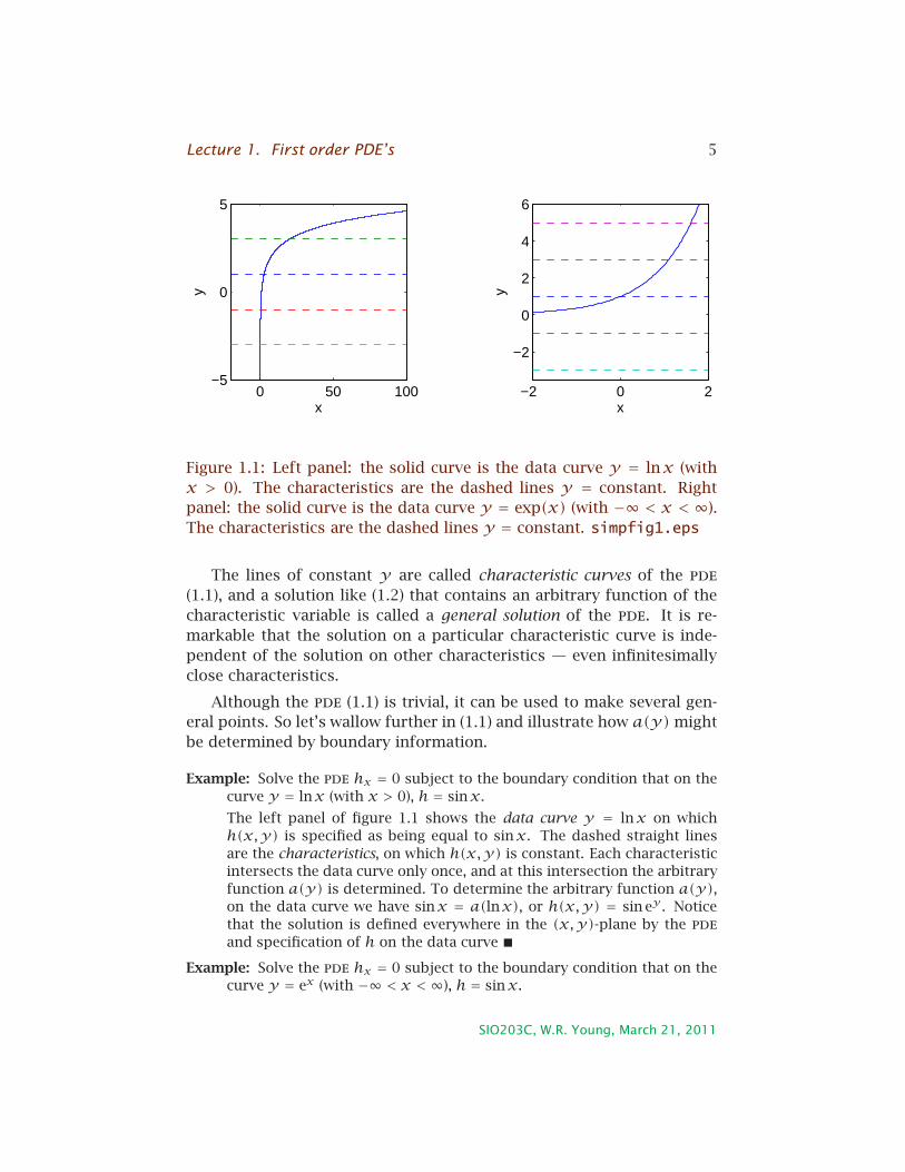
Figure 1.1: Left panel: the solid curve is the data curve y = lnx (with
x > 0). The characteristics are the dashed lines y = constant. Right
panel: the solid curve is the data curve y = exp(x) (with −∞ < x < ∞).
The characteristics are the dashed lines y = constant. simpfig1.eps
The lines of constant y are called characteristic curves of the pde
(1.1), and a solution like (1.2) that contains an arbitrary function of the
characteristic variable is called a general solution of the pde. It is re-
markable that the solution on a particular characteristic curve is inde-
pendent of the solution on other characteristics — even infinitesimally
close characteristics.
Although the pde (1.1) is trivial, it can be used to make several gen-
eral points. So let’s wallow further in (1.1) and illustrate how a(y)might
be determined by boundary information.
Example: Solve the pde hx = 0 subject to the boundary condition that on the
curve y = lnx (with x > 0), h = sinx.
The left panel of figure 1.1 shows the data curve y = lnx on which
h(x,y) is specified as being equal to sinx. The dashed straight lines
are the characteristics, on which h(x,y) is constant. Each characteristic
intersects the data curve only once, and at this intersection the arbitrary
function a(y) is determined. To determine the arbitrary function a(y),on the data curve we have sinx = a(lnx), or h(x,y) = sin ey . Notice
that the solution is defined everywhere in the (x,y)-plane by the pde
and specification of h on the data curve
Example: Solve the pde hx = 0 subject to the boundary condition that on the
curve y = ex (with −∞ < x < ∞), h = sinx.
SIO203C, W.R. Young, March 21, 2011

Lecture 1. First order PDE’s 6
In the right panel of Figure 1.1 we show the data curve y = exp(x)and the dashed straight lines which are the characteristics of the pde
hx = 0. In this case, only the characteristics in the upper half plane
intersect the data curve. Consequently the data determines the arbitrary
function a(y) only in the upper half plane. In the lower half plane the
function a(y) is still arbitrary: the characteristics in the lower half plane
don’t find the data curve. Thus in this example we have incomplete
determination of h(x,y).
Focussing then on the upper-half plane, at the intersection of the char-
acteristics with the data curve we have sinx = a(ex), so in the region
y > 0 we have h(x,y) = sin lny . We say that the domain of definition
of the solution is the upper half plane y > 0
Example: Solve pde hx = 0 subject to the boundary on y = 0, h = sinx.
In this case there is no solution: the pde says that h is constant on
every line of constant y , and the boundary condition contradicts this
on the particular line y = 0. If the boundary condition is changed to
h = π on y = 0 then there is no longer an inconsistency — in this case
h(x,0) = π . But h(y) remains undetermined for y ≠ 0
Example: Solve the pde hx = 0, subject to the boundary condition that h = xon the circle x2 +y2 = 1.
You should draw1 the circle and the lines of constant y . In the regions
where |y| > 1 the lines of constant y don’t intersect the circle. Thus the
boundary condition supplies no information in these regions. All we can
say is that h(x,y) = a(y), with a(y) still arbitrary if |y| > 1.
Inside the circle x2+y2 = 1 the pde has no solutions, because h(x,y) =a(y) can’t satisfy the boundary condition at both
x = +√
1− y2 and x = −√
1−y2 . (1.4)
We might say that in the region x2+y2 < 1, the boundary information is
inconsistent with the pde and there is no solution. An alternative point
of view is that inside the circle the solution is double valued. That is at
each point (x,y) one has a solution
h+(x,y)def= +
√1−y2 , (1.5)
and a second solution
h−(x,y)def= −
√1−y2 . (1.6)
1When I first starting writing these notes I felt obliged to draw all figures. This is
a lot of work. However I’ve been told by Roger Samelson that the best educational
strategy is to leave out most of the figures, and insist that students provide these
themselves. Thus omission of some essential figures is a feature, rather than a bug.
SIO203C, W.R. Young, March 21, 2011

Lecture 1. First order PDE’s 7
We need more information (e.g., some physical context) to make sense
of this situation.
In the remainder of the plane, where |y| < 1 and x2 + y2 > 1, we can
say that the solution is
h(x,y) =
+√
1−y2 , if x ≥ +√
1−y2;
−√
1−y2 , if x ≤ −√
1−y2.(1.7)
Even this construction requires a little bit of reformulation: we’re saying
that the solution in the region x > +√
1− y2 ignores that part of the data
curve in the region with x < 0, and vice versa. This sounds reasonable,
but it is not strictly obvious from the bare formulation of the pde plus
data
The transport equation
The transport equation for the unknown function h(x,y) is
ahx + bhy = 0 , where a and b are constants. (1.8)
The pde in (1.1) is the special case a = 1 and b = 0.
The transport equation is a simple pde that occurs frequently in ap-
plications. By inspection, the general solution of the transport equation
is
h(x,y) = f(bx − ay) , (1.9)
where f(p) is an arbitrary function.aaa = ax+ by
We can write the transport equation as
aaa···∇∇∇h = 0 , where aaa ≡ (a, b). (1.10)
In this form we interpret (1.8) geometrically as saying that the direc-
tional derivative of u(x,y) along the vector aaa is zero. We say that h is
transported along the vector aaa. Then the variation of h must be in the
direction orthogonal to aaa i.e.,
h = f(ppp···xxx) , (1.11)
where ppp is any vector orthogonal to aaa. In writing the general solutionppp···aaa = 0(1.9) we happened to use ppp = aaa× z = (b,−a).
SIO203C, W.R. Young, March 21, 2011

Lecture 1. First order PDE’s 8
This observation is the key to solving the transport equation in higher
dimensions e.g., in three dimensions we can interpret
ahx + bhy + chz = 0 (1.12)
as saying that the directional derivative of h(x,y, z) along the vector
aaa ≡ (a, b, c) is zero. Therefore the general solution of the three-dimensional
transport equation is
h = f(ppp···xxx,qqq···xxx) , (1.13)
where ppp and qqq are any two linearly independent vectors orthogonal to aaaand f is an arbitrary function with two arguments.
Notice that the solution of the pde (1.12) is a three-dimensional sur-
face embedded in a four-dimensional space.
Example: Find a general solution of
xhx −yhy = 0 . (1.14)
If we change variables to ξ = lnx and η = lny then the equation is
transformed to the transport equation
hξ − hη = 0 . (1.15)
The general solution is that
h = f (ξ + η) = f(ln(xy)
)= g(xy) , (1.16)
where f and g are arbitrary functions
1.2 Arbitrary functions
Now let’s consider a slightly more complicated example of arbitrary
functions. What do all of the following functions
f1(x,y) = x4 + 4(x2y +y2 + 1) ,
f2(x,y) = sinx2 cos 2y + cosx2 sin 2y ,
f3(x,y) =x2 + 2y + 2
3x2 + 6y + 5, (1.17)
have in common? Each fn is a function of the simpler function
p(x,y) ≡ x2 + 2y . (1.18)
SIO203C, W.R. Young, March 21, 2011

Lecture 1. First order PDE’s 9
Specifically
f1 = p2 + 4 , f2 = sinp , f3 =p + 2
3p + 5. (1.19)
This also means that the contours of the functions fn(x,y) in the (x,y) AKA the ‘level sets’ of fn
plane all coincide with the contours of the simple function p(x,y). Yet
another consequence is that a ‘scatterplot’ of say f1 against f2 produces
a curve (rather than a cloud) in the (f1, f2)-plane.
Since p(x,y) is a solution of the pde
hx − xhy = 0 , (1.20)
all of the fn’s are also solutions of the pde above. We can check this by
substitution. Suppose that h is an arbitrary function of p. Then
h(p)x = pxdh
dp, and h(p)y = py
dh
dp(1.21)
so that
hx − xhy =dh
dp
(px − xpy
)= 0 . (1.22)
In fact the general solution of the pde (1.20) is that h(x,y) an arbitrary
function of x2 + 2y .
Since the function p(x,y) is so central to the solution of (1.20), let
us “change coordinates” from x and y to p(x,y) and q(x,y). At the recall
p(x,y) ≡ x2 + 2ymoment q(x,y) is just some other unspecified function of x and y(your choice).
We recall the rule for converting derivatives
∂x = px∂p + qx∂q = 2x∂p + qx∂q ,∂y = py∂p + qy∂q = 2∂p + qy∂q . (1.23)
These relations imply
∂x − x∂y = (qx − xqy)∂q . (1.24)
Thus, provided that we can find a q(x,y) satisfying For example, q = x.
xqy − qx ≠ 0 , (1.25)
we can rewrite (1.20) in terms of (p, q) as simply
hq = 0 . (1.26)
This should remind you of (1.1) — the solution is that h(x,y) is a pos-
sibly discontinuous arbitrary function of p(x,y).
SIO203C, W.R. Young, March 21, 2011

Lecture 1. First order PDE’s 10
Example: Solve
ux − xuy = ey . (1.27)
We change coordinates to p = x2 + 2y and q = x. In these new coordi-
nates
y = 12p − 1
2q2 , and ∂x − x∂y = ∂q . (1.28)
Thus the pde is
uq = e12p−1
2q2
, or u = e12p∫ q
0e−1
2s2
ds + f (p) , (1.29)
where f is an arbitrary function. We can now rewrite this in terms of the
original variables x and y :
u(x,y) = ey+1
2x2∫ x
0e−1
2 s2
ds + f (x2 + 2y) . (1.30)
This is the general solution of the pde. The final step is to check by
substitution that this solution works (do it)
Example: Solve ux − xuy = ey with the boundary condition u(0, y) = 0.
The first step is to draw the characteristics curves on which p = x2+2yis constant. Then you have to figure out where (or if) these character-
istics intersect the curve on which the boundary condition is specified
(that’s the y-axis in this problem). This drawing should convince you
that every characteristic intersects the y-axis exactly once.
Applying the boundary condition to the general solution in (1.30) we
have
0 = ey∫ 0
0e−1
2s2
ds︸ ︷︷ ︸
=0
+f (y) . (1.31)
Thus f = 0 in (1.30) does the trick in this case.p = x2 + 2y
Example: Solve ux − xuy = ey with the boundary condition u(x,0) = 0.
Now the boundary condition is applied on the x-axis. But characteristics
with p(x,y) < 0 don’t intersect the x-axis. So in the region where p < 0
the function f in (1.30) is still arbitrary.
Characteristics with p(x,y) > 0 intersect the x-axis twice, at x = ±√p.
This means that the boundary data is inconsistent with the pde: there is
no solution to this problem in the region where p > 0.
Suppose we ignore the red flag raised by the double intersection and try
to determine f by insisting that
0 = e12x
2∫ x
0e−1
2 s2
ds + f (x2) . (1.32)
SIO203C, W.R. Young, March 21, 2011
Lecture 1. First order PDE’s 11
It seems that
f (p) = −e12p∫ ±√p
0e−1
2s2
ds . (1.33)
But if we take the +√p in the upper limit of the integral then we satisfy
the boundary condition on x > 0, but unfortunately not on x < 0 (and
vice versa).
If we modify the boundary condition to u(x > 0,0) = 0 then we’re in
business. The solution to the modified problem is If x is real√x2 = |x|
u = ey+1
2x2
∫ x
0e−1
2 s2
ds −∫ +√2y+x2
0e−1
2 s2
ds
. (1.34)
Notice that u(x < 0, y) ≠ 0.
1.3 The Jacobian
Suppose u(x,y) and v(x,y) are differentiable functions of x and y .
Then a necessary and sufficient condition for the existence of a func-
tional relation,
φ(u,v) = 0 , or perhaps u = A(v), (1.35)
is that the Jacobian∂(u,v)
∂(x,y)≡ uxvy −uyvx (1.36)
is zero. For instance, in the example surrounding (1.1), one can show
that∂(p,un)
∂(x,y)= 0 . (1.37)
Let’s prove this algebraically by differentiating φ(u,v) = 0 with re-
spect to x and y :
uxφu + vxφv = 0 , and uyφu + vyφv = 0 . (1.38)
Eliminating the derivatives φu and φv we obtain
∂(u,v)
∂(x,y)= 0 . (1.39)
Therefore vanishing of the Jacobian is necessary for the existence of a
function relation between u and v. The condition is also sufficient.
SIO203C, W.R. Young, March 21, 2011

Lecture 1. First order PDE’s 12
The geometric interpretation of the condition (1.39) is that u(x,y)and v(x,y) are functionally related if their contours coincide, which is
equivalent to saying that ∇∇∇u and ∇∇∇v are parallel at every point. Now
recall that
z·(∇∇∇u×∇∇∇v) = |∇∇∇u||∇∇∇v| sinθ (1.40)
where θ is the angle between ∇∇∇u and ∇∇∇v. So ∇∇∇u and ∇∇∇v are parallel
at a point if and only if |∇∇∇u| ≠ 0, |∇∇∇v| ≠ 0 and θ = 0. But it is easy to
verify that
z·(∇∇∇u×∇∇∇v) = ∂(u,v)∂(x,y)
. (1.41)
Solving (really) simple pde’s with Jacobians
One way of solving a pde such as
(cosy)uy + (x siny)ux = 0 (1.42)
is by recognizing a thinly disguised Jacobian:
(x cosy)xuy − (x cosy)yux = 0 . (1.43)
Thus the general solution is that u is an arbitrary function of x cosy .
But unfortunately not all pdes of the form
a(x,y)ux + b(x,y)uy = 0 (1.44)
are disguised Jacobians: for the lhs to be a Jacobian one must have that
ax + by = 0.
Example Find the general solution of
(x + 2y)ux − (6x + y)uy = 0 (1.45)
by showing that the lhs is a Jacobian.
If the lhs is a Jacobian then there is a function v(x,y) such that
vy = x + 2y , ⇒ vyx = 1 . (1.46)
But we also require
vx = 6x +y , ⇒ vxy = 1 . (1.47)
SIO203C, W.R. Young, March 21, 2011

Lecture 1. First order PDE’s 13
The equation passes the test so we know that the object of our desire,
v(x,y), exists. Now we proceed to uncover v by integration
vx = 6x + y , ⇒ v = 3x2 + xy +A(y) ,vy = x + 2y , ⇒ v = xy +y2 + B(x) . (1.48)
Subtracting our different expressions for v we soon see that
v = 3x2 + xy + y2 + constant . (1.49)
Thus the solution is that u is an arbitrary function of 3x2 + xy +y2
Example Is the pde
(x + 2y)wx + (6x +y)wy = 0 . (1.50)
a Jacobian?
Since (x + 2y)x + (6x +y)y ≠ 0, the lhs above is not a Jacobian
In next section we’ll develop the method of characteristics to solve
non-Jacobian pdes such as (1.50).
1.4 The method of characteristics
Consider some function h(x,y) which you can visualize as the height
of a surface above the (x,y) plane. If you move around on the (x,y)-plane following a curve y = y(x) then you will observe changes in hboth because x changes and also y changes. In fact, the total derivative
of h(x,y) following this moving point is
d
dxh(x,y) = hx +
dy
dxhy . (1.51)
We will use this result again and again and again.
The pde
hx + (x +y)2hy = 0 (1.52)
is not a disguised Jacobian and one can’t guess the solution. However
comparing (1.52) and (1.51) we see that if we move in the (x,y) plane
along a path P satisfying
dy
dx= (x +y)2 (1.53)
SIO203C, W.R. Young, March 21, 2011

Lecture 1. First order PDE’s 14
then on P the pde impliesdh
dx= 0 . (1.54)
This means that h(x,y) is a constant on the path i.e., P is a contour or
level-set of the function h(x,y).
Now it is easy to integrate (1.53) and we find Let v ≡ x +y so
dv
dx= 1+ v2
and then separation
gives
x +y = tan(x + ξ) .
ξ(x,y) = tan−1(x +y)− x (1.55)
where ξ is a “constant of integration”; curves of constant ξ are shown
in Figure 1.2. Regarding ξ is function of x and y defined by (1.55), the
solution of (1.52) is
h(x,y) = an arbitrary function of ξ(x,y) . (1.56)
Thus the curves in Figure 1.2 are the “level sets” or the “contours” of the
function h(x,y). The collection of special paths P along which a pde
collapses to an ode such as (1.54) are characteristics. We’ll give a more
careful definition in the next few lectures.
Example Find the solution of
vx + (x +y)2vy = 1 , (1.57)
subject to v(x,−x) = 0.
On the path defined by (1.53) the pde is
dv
dx= 1 , or v = x + f
(tan−1(x +y)− x
). (1.58)
This is the general solution. The arbitrary function f is determined by
the boundary condition that v = 0 on the curve y + x = 0:
0 = x + f (−x) . (1.59)
This implies that f (s) = s and v = tan−1(x + y). Figure 1.2 shows that
there is a unique intersection, and the characteristics fill up the whole
plane. Therefore in this problem the domain of definition is the entire
(x,y)-plane.
Notice that in this example the solution v is not constant on character-
istics: the defining quality of characteristics is that the variation of v is
determined by solving an ode
SIO203C, W.R. Young, March 21, 2011

Lecture 1. First order PDE’s 15
x
y
−2 −1.5 −1 −0.5 0 0.5 1 1.5 2−2
−1.5
−1
−0.5
0
0.5
1
1.5
2
Figure 1.2: The solid curves
are the characteristics in
(1.55). The dashed line
y + x = 0 intersects
each characteristic once.
atanchar.eps
Example Find the general solution of the non-Jacobian pde
(x + 2y)wx + (6x +y)wy = 0 . (1.60)
On the paths defined bydy
dx= y + 6x
2y + x (1.61)
the pde collapses to an ode:
dw
dx= 0 . (1.62)
That is,w is constant on the characteristics determined by solving (1.61).
To integrate (1.61 we turn to section 1.7 of BO and observe that the
equation is scale invariant i.e., the ode is unchanged if y → ay and
x → ax. Following the BO recipe, we first substitute y = xY(x) so that
xdY
dx+ Y = Y + 6
2Y + 1, (1.63)
and if λ = lnx then
dY
dλ= 6− 2Y 2
1+ 2Y, or
1+ 2Y
6− 2Y 2dY = dλ . (1.64)
To do the Y -integral I used mathematica, and obtained
√3− 6
12ln(√
3+ Y)−√
3+ 6
12ln(√
3− Y)= λ+ c . (1.65)
SIO203C, W.R. Young, March 21, 2011

Lecture 1. First order PDE’s 16
The constant of integration is c. But c is is also the label of the charac-
teristic, or equivalently w is constant along curves of constant c. Thus
w is an arbitrary function of
ec = x−1
(√3+ y
x
)√3−612
(√3− y
x
)−√
3+612
(1.66)
1.5 Some books
Four good general texts on pdes written by applied mathematicians are:
CP Partial Differential Equations: Theory and Technique by G.F. Carrier
& C.E. Pearson.
Z Partial Differential Equations of Applied Mathematics by E. Zauderer.
K Partial Differential Equations: Analytic Solution Techniques by J. Kevorkian.
Sn Elements of Partial differential Equations by I.N. Sneddon.
CP and Sn have the advantage of brevity. Z is a leisurely intoduction,
with lots of problems. The first two chapters of Sn are a good introduc-
tion to the geometric theory of first-order pde’s.
There are several ‘math methods’ books written by physicists for
physicists which contain a lot of material on pde’s. Four good ones are:
So Partial Differential Equation by A. Sommerfeld.
MW Mathematical Methods of Physics by J. Matthews & R.L. Walker.
W Mathematical Analysis of Physical Problems by P.R. Wallace.
MF Methods of Theoretical Physics; Part I and II by P.M. Morse & H. Fes-
hbach.
MF is useful as a compendium of formulas and methods. So is a very
readable classic.
Two other classic textbooks on wave dynamics, characteristics and
much more are:
W Linear and Nonlinear Waves by G.B. Whitham.
SIO203C, W.R. Young, March 21, 2011

Lecture 1. First order PDE’s 17
ZR Physics of Shock Waves and High-Temperature Hydrodynamic Phe-
nomena by Ya. B. Zeldovich & Yu. P. Raizer.
W is a tough book, but well worth the effort. The first chapter of ZR is a
good introduction to gas dynamics and the wave equation.
General texts on mathematical methods are:
BO Advanced Mathematical Methods for Scientists and Engineers by C. Ben-
der & S.A. Orszag.
JJ Methods of Mathematical Physics by H. Jeffreys & B.S. Jeffreys.
Useful handbooks are:
AS Handbook of Mathematical Functions with Formulas, Graphs and Math-
ematical Tables by M. Abramowitz & I. Stegun.
GR Tables of Integrals, Series and Products by I.S. Gradshteyn & I.M.
Rhyzik. (The recent editions are edited by A. Jeffrey & D. Zwill-
inger).
1.6 Problems
Problem 1.1. Evaluate the derivative
(∂x − x∂y) ln
(f1f3
1− sin1/3(f2)
)cos(x −y) ,
where the functions fn(x,y) are defined in (1.17)
Problem 1.2. Find the general solution of ux − xuy = 1.
Problem 1.3. Find the general solution of ux−xuy = f ′(x)g(x2+2y).Here f and g are arbitrary functions and f ′ is the derivative of f .
Problem 1.4. (i) Find the solution, and where in the (x,y)-plane there
is a solution (i.e., the domain of definition), of the pde hx − xhy = 0,
subject to the boundary condition that h(x,x2/2) = x. (ii) Same pde,
but with the boundary condition h(x,x2/2) = x2.
SIO203C, W.R. Young, March 21, 2011

Lecture 1. First order PDE’s 18
Problem 1.5. Consider the transport equation hx+hy = 0 with the data
h(x,x2) = f(x) i.e., h is specified on the parabola y = x2 as equal to a
specified function f(x). Discuss the solution of this problem — where
in the (x,y)- plane is the solution defined?
Problem 1.6. Find an example of a function u(x,y) which is discontin-
uous at (x,y) = (0,0), even though all directional derivatives exist at
(x,y) = (0,0).
Problem 1.7. (i) Spot the Jacobian and find the general solution of the
following pde
(x +y)fx − (2x +y)fy = 0 .
(ii) Consider the pde
(ax + by)gx + (cx + dy)gy = 0 ,
where a, b, c and d are all constants. Find the condition ensuring that
this pde is a Jacobian, and then find the general solution.
Problem 1.8. Is the lhs of
ex cosy ux − ex siny uy = 0 ,
a Jacobian? How about
(cosx coshy − sinx sinhy)ux − (sinx sinhy + cosx coshy)uy = 0 ?
Problem 1.9. Let
f(x,y) ≡∫∞
0
t exp[−y√
1+ t2] sinxt√1+ t2
dt .
Use integration by parts to show that
f(x,y) = xy
∫∞
0exp[−y
√1+ t2] cosxt dt .
Next, differentiate with respect to x and y and show that
fy =[(y/x)f
]x .
Show that the solution of this pde is f = xg(x2 + y2) where g is an
arbitrary function. Find a simple form for g. (From CP.)
SIO203C, W.R. Young, March 21, 2011

Lecture 1. First order PDE’s 19
Problem 1.10. Find a solution of the pde
uxxuyy −u2xy = 0 , u(x,0) = 1
2x2 , uy(x,0) = x .
(Hint: look for a Jacobian.)
Problem 1.11. Consider the three functions
φ ≡ x +y + z , θ = x2 +y2 + z2 , χ ≡ xy +yz + zx .
(i) Show that one of these can be written as a function of the other two.
(ii) Find a pde of the form
aux + buy + cuz = 0 , with a, b and c functions of (x,y, z) ,
whose general solution is that u is an arbitrary function of φ and θ.
Problem 1.12. Suppose you are given three function of (x,y, z) (e.g.,
as in problem 1.11). Find a three-dimensional generalization of the Ja-
cobian criterion which tests if such a functional relation exists between
the three. Give both an algebraic proof and a geometric interpretation.
Hint: Denote the three given functions byu(x,y, z), v(x,y, z) andw(x,y, z).Suppose that there is some unknown functional relation
Φ(u,v,w) = 0 ,
connecting u, v and w. Differentiating with respect to x, y and z we find
uxΦu + vxΦv +wxΦw = 0 ,
uyΦu + vyΦv +wyΦw = 0 ,
uzΦu + vzΦv +wzΦw = 0 .
This is 3×3 set of linear equations for the three unknowns (Φu,Φv ,Φw). If the
only solution is (Φu,Φv ,Φw) = (0,0,0) then there is no nontrivial functional
relation.
Problem 1.13. Reduce the following pde’s to the transport equation and
construct the general solution:
yux+xuy = 0 , xux+yuy = 0 , uy +exux = u , uy +(xu)x = 0.
Solution: For the first example, divide by xy make the change of variables
ξ = x2 and η = y2, so that the equation becomes
uξ +uη = 0 ⇒ u = f (ξ − η) = f (x2 −y2) .
This problem illustrates how one can sometimes quickly beat simple pde into
a soluble form by making a change of variables
SIO203C, W.R. Young, March 21, 2011

Lecture 1. First order PDE’s 20
Problem 1.14. Find the general solution of the pdes
a(x)ux + b(y)uy = 0 ,
a(x)vx + b(y)vy + c(z)vz = 0 .
Problem 1.15. Find the general solution of the pde ux + (x+y)uy = 0.
Check your answer by substitution.
Problem 1.16. Find the general solution of the pde ux+(x+y)2uy = u.
Check your answer by substitution.
Problem 1.17. (i) Find the general solution of the pde xyux + uy = 0.
(ii) Find the solution satisfying the boundary data u(x,0) = x. What is
the domain of definition of this solution?
Problem 1.18. Consider the pde ux + βuy = 0 with the boundary con-
dition u(x,x − 1) = x. Find the solution and state any condition which
must be imposed on the constant β in order for the solution to exist.
Problem 1.19. Find the general solution of
aux + buy + cuz = 0 , and pux + quy + ruz = 0 .
Above a, b etc. are all constants.
SIO203C, W.R. Young, March 21, 2011

Lecture 2
Linear evolution equations
In this lecture we discuss some relatively simple applications of the
method of characteristics to linear evolution problems. “Evolution” means
changing in time — so one of our independent variables in this lecture
is time t.
2.1 Conservation laws
First-order pde’s arise in applications frequently as a result of conser-
vation laws. The fundamental idea here is simple: count the amount of
stuff in some control volume and then:
d
dt[Amount of Stuff] = [ Stuff entering]− [Stuff leaving] . (2.1)
Consider traffic on the northbound lanes of a highway as an example.
We use the coordinate x to denote distance along the road. The density,
ρ(x, t), is the number of cars per length. In the interval a < x < b the
total number of cars is
Number of cars in the interval a < x < b =∫ b
aρ(x, t)dx. (2.2)
We have made the continuum approximation by assuming that there is
a well defined density which is a smooth function of position. If a car
is 5 meters long it makes no sense in (2.2) to pick an interval of length
1 meter. The introduction of the density ρ(x, t) requires a separation
21

Lecture 2. Linear evolution equations 22
in length scales between the distance over which ρ(x, t) changes appre-
ciably (e.g. one kilometer) and the distance between cars (e.g. a few
meters).
We apply the principle in (2.1) by picking an interval of highway a <x < b, and counting the number of cars which pass x = a in a time dt.Thus we define the flux (cars per second passing x = a) as f(a, t). We
can do the same at the other end of the control length and so determine
f(b, t). We are ignoring off-ramps and on-ramps which introduce cars
into the middle of (a, b). Then (2.1) tells us that
d
dt[Number of cars in the interval a < x < b] = f(a, t)− f(b, t). (2.3)
In other words
d
dt
∫ b
aρ(x, t)dx + f(b, t)− f(a, t) = 0 . (2.4)
Letting a → b in (2.4), with x sandwiched in the middle, we obtain the Assumption: ρ is
continuous and fdifferentiable.
differential statement of the conservation law:
ρt + fx = 0 . (2.5)
If we can find a relation between f(x, t) and ρ(x, t) then the conserva-
tion law in (2.5) is a pde for the density of traffic.
The linear advection equation
Suppose, for example, that all of the drivers are law abiding so that
everyone is moving at exactly c = 65mph. In this unrealistic case we get
a simple and important example of a first order pde: The linear advection
equation
f = cρ in (2.5) ⇒ ρt + cρx = 0 . (2.6)
The boxed equation is the linear advection equation — you’ll notice it’s
a special case of the transport equation from lecture 1.
There are two ingredients in this argument. There is the conservation
law in (2.3) and the connection between flux and density, namely f = cρ.
Once we accept the continuum approximation the integral form of the
conservation law in (2.3) is unassailable. But the flux-density relation
between might be a matter of debate. In realistic cases, such as traffic
SIO203C, W.R. Young, March 21, 2011

Lecture 2. Linear evolution equations 23
-2 0 2 4 6 80
2
4
6
8
0
1
2 t
x
ρ
Figure 2.1: The solution (2.8) of the advection equation. The location of
the Gaussian pulse moves with constant velocity c. gaussWave.eps
flow, the connection between flux and density has to be determined em-
pirically and the resulting pde is nonlinear. Moreover, as we’ll see later,
the transition from the integral law (2.3) to the differential law (2.5) can
also be difficult: ρ can spontaneously develop discontinuities (shocks).
By now you should be able to write down the general solution of (2.6)
on auto-pilot:
ρ(x, t) = q(x − ct) , (2.7)
where q is arbitrary function. To determine q we need a combination of
initial and boundary conditions. The simplest case is the initial value
problem in which q is determined by specifying an initial condition
which applies for all x. For example:
ρ(x,0) = exp(−x2) , ⇒ ρ(x, t) = exp[−(x − ct)2] . (2.8)
The pulse preserves its shape and moves with constant velocity c (see
the top panel of figure 2.1). This is a travelling wave solution of the pde
in (2.6).
2.2 A recipe for semilinear evolution equations
We can solve a first-order pde in the form1
ρt + c(x, t)ρx = s(x, t, ρ) , ρ(x,0) = ρ0(x) , (2.9)
1We call this a “semilinear” equation because the right hand side is a possibly non-
linear function of ρ.
SIO203C, W.R. Young, March 21, 2011

Lecture 2. Linear evolution equations 24
using the following recipe:
• define a characteristic coordinate ξ(x, t) by
dx
dt= c(x, t) , x(ξ,0) = ξ ; (2.10)
• sketch the characteristic diagram;
• find ρ(ξ, t) by integrating the ode
dρ
dt= s[x(ξ, t), t, ρ] , ρ(ξ,0) = ρ0(ξ) ; (2.11)
• eliminate ξ in favor x and t;
• check by substitution.
Conservation versus non-conservation
Let us apply the recipe and solve the pde
ρt − (xρ)x = 0 , ρ(x,0) = e−x2. (2.12)
Notice that this pde has the form of a conservation law i.e., the flux is
−xρ. You can imagine a bunch of particles moving along the x-axis with
speed c = −x, and density ρ(x, t). Since particles don’t disappear, the
total number of particles — obtained by integrating ρ(x, t) over x —
must be conserved.
Let’s do this explicitly. We integrate (2.12) over a < x < b and obtain
d
dt
∫ b
aρ dx
︸ ︷︷ ︸Change in the amount of stuff
= [xρ]ba︸ ︷︷ ︸stuff in - stuff out
. (2.13)
ρ flows in and out of (a, b) at the end points and that accounts for all
changes in the total amount of ρ in the interval.
Equation (2.12) above can be written in the standard form (2.9):
ρt − xρx = ρ , (2.14)
SIO203C, W.R. Young, March 21, 2011

Lecture 2. Linear evolution equations 25
and we are off to the races. First, we obtain the characterstic coordinate
dx
dt= −x , x(0, ξ) = ξ ⇒ x = ξe−t . (2.15)
Next we solve the ode
dρ
dt= ρ , ρ(ξ,0) = e−ξ
2, ⇒ ρ(x, t) = et−ξ
2. (2.16)
Notice that ξ is a ‘constant on characteristics’ so when we integrate the
ode in (2.16) the constant of integration is an arbitrary function of ξ. To
determine this arbitrary function of ξ we look at at t = 0. At the initial
instant ξ = x so that the initial condition for the ode (2.16) follows from
(2.12): ρ0(ξ) = exp(−ξ2).
In the next step of the recipe we eliminate ξ = x exp(t):
ρ(x, t) = exp(t − e2tx2
). (2.17)
Finally, we check by substitution that this really is the solution of the
pde (2.12).
Notice if the initial condition in (2.12) is changed to ρ(x,0) = ρ0(x)then the solution is just ρ(x, t) = etρ0(etx). From this solution we can
verify that conserves particles are conserved i.e., you should show that
m ≡∫∞
−∞ρ(x, t)dx (2.18)
is constant (independent of time). We know this even before we go to
the trouble of solving the equation, but it is interesting to see how it all
works out.
Let’s dwell further on the difference between conservation and non-
conservation. Unlike (2.12), the pde
θt − xθx = 0 , (2.19)
is not a conservation equation. Notice what happens if we integrate-by-
parts over a < x < b:
d
dt
∫ b
aθ dx
︸ ︷︷ ︸Change in the amount of stuff
= [xθ]ba︸ ︷︷ ︸stuff in - stuff out
−∫ b
aθdx
︸ ︷︷ ︸source of stuff
. (2.20)
θ-stuff appears out of thin air in the middle of (a, b).
SIO203C, W.R. Young, March 21, 2011

Lecture 2. Linear evolution equations 26
2.3 Entry on the half-line
Now we turn to problems defined on the half-line x ≥ 0. Think of x = 0
as the beginning of a highway and suppose we count the number of cars
entering at x = 0. If this entry rate increases then there is a bulge in
the traffic density, ρ, which propagates down the roadway. This bulge
is a signal indicating changes in the upstream conditions. In our sim-
plest model, with constant speed c, the signal from x = 0 reaches x at
time x/c. Another example might be one-dimensional radiative transfer:
ρ(x, t) is the density of photons moving along the positive half of the
x-axis with the speed of light c. The source at x = 0 is a laser emitting
new photons.
Note carefully we’re discussing entry problems. That is
c > 0 (2.21)
so that cars or photons are entering at x = 0. We’ll come back at the end
of this section and discuss the more subtle exit problem in which c < 0.
To formulate the problem mathematically, denote the rate at which
cars enter at x = 0 by R(t) (cars per second). The conservation equation
is our old friend the linear advection equation
ρt + cρx = 0 . (2.22)
For a pde model we specify both an initial condition
ρ(x,0) = F(x) , for x > 0 , (2.23)
and a boundary condition
cρ(0, t) = R(t) , for t > 0 . (2.24)
Notice the dimensions — R is cars per second, ρ is cars per meter and cis meters per second.
To solve this problem it is essential to draw the (x, t)-plane and the
family of curves on which ρ(x, t) is constant. These characteristics are
the lines The general solution of
(2.22) is
ρ = q(x − ct) = q(ξ).x − ct = ξ , (2.25)
where ξ is the intercept of the characteristic with the x-axis (see figure
2.1). You can think of ξ as the name of each member of the family of
SIO203C, W.R. Young, March 21, 2011

Lecture 2. Linear evolution equations 27
ξ1
x-ct= ξ 1
x-ct= ξ 2
x
t
t=- ξ2/c
Figure 2.2: The (x, t)-diagram, or characteristic diagram, for the sig-
naling problem. The shaded region is x − ct = ξ > 0, in which the
solution is determined by information from t = 0. The unshaded region
is x − ct = ξ < 0, in which the solution is determined by information
from x = 0. signal.eps
lines in figure 2.2. The spacetime diagram in figure 2.2 is the character-
istic diagram of the pde.
The characteristics in the shaded region have ξ > 0 and they intersect
the x-axis where (2.23) applies. Thus in the shaded region ρ = F(x−ct):the signal from x = 0 has not had time to arrive, and the solution is
identical to that of the initial value problem. The characteristics in the
unshaded region intercept the t-axis where (2.24) applies. In this region
the signal from x = 0 has finally arrived and we determine q(x − ct)from The general solution of
(2.22) can also be
written ρ = p(t − x/c).x = 0 : cq(−ct) = R(t) ⇒ q(s) = c−1R(−s/c) . (2.26)
Thinking carefully about this argument, you’ll see that characteristics
are spacetime curves along which signals propagate. To determine the
arbitrary function, q, we follow each characteristic till we hit the bound-
ary of the spacetime domain.
Summarizing, the solution of this “signaling” problem is
ρ(x, t) =
F(x − ct) , if x − ct > 0,
c−1R(t − x/c) , if x − ct < 0.(2.27)
In general F(0) ≠ R(0) so the solution might be discontinuous on the
line x = ct. For instance, suppose ρ(x,0) = 0 and R is a constant. Then
the solution is ρ(x, t) = c−1RH(ct − x) where H is the Heaviside step
function.
SIO203C, W.R. Young, March 21, 2011

Lecture 2. Linear evolution equations 28
The exit problem, c < 0
If you redraw Figure 2.2 with c < 0 then you immediately see that the
characteristics intersect the boundary twice: the lines of constant x− ctintersect both the positive x-axis and the positive t-axis. Consequently
one if arbitrarily specifies both F(x) and R(t) then usually the problem
has no solution.
In discussing this non-existence one must be sensitively aware of
the distinction between the mathematical formulation and the physical
situation. The former is an approximation or idealization of the latter.
If one is not aware of the physical motivation then one declares that the
pde plus boundary/initial condition has no solution, and that’s the end
of the matter. But thinking of the original motivation for this model
in terms of traffic flow or photons it seems clear, to me at least, that
one can prescribe the initial condition on the positive x-axis, and one
cannot prescribe the exit condition on the positive t-axis. The exit at
x = 0 takes what it gets and doesn’t complain. If the exit does complain
(e.g., if some fraction of the incident photons are reflected back into the
domain) then one must reformulate the physical problem to account for
this complication.
Example: Formulate a half-line (x > 0) model in which photons move in both
directions with speed ±c. Assume that all photons with speed −c inci-
dent on x = 0 are reflected back with speed +c. Photons with speed +care also emitted at x = 0 at a rate R(t).
We need two densities, ρ+(x, t) for photons with +c and ρ−(x, t) for
photons with speed −c < 0. The pdes are
ρ+t + cρ+x = 0 , ρ−t − cρ−x = 0 . (2.28)
The boundary condition at x = 0 is
cρ+(0, t) = R(t)+ cρ−(0, t) . (2.29)
We must also supply initial conditions for ρ+ and ρ− on the half-line. As
a sanity check, you should show that
d
dt
∫∞
0ρ+(x, t)+ ρ−(x, t)dx = R(t) (2.30)
SIO203C, W.R. Young, March 21, 2011

Lecture 2. Linear evolution equations 29
2.4 Age-Stratified Populations
Let us give another example of a context in which the half-line linear
advection equation, (2.6) arises. To characterize the age structure of the
population of San Diego at t = 0 we use a histogram:
h0(a)da = the number of people with age a ∈ (a,a+ da) at t = 0.
(2.31)
The age-coordinate, a, is strictly positive so that the histogram lives on
the half-line a > 0.
Suppose for a moment that this population is closed — we ignore
births, deaths and immigration. Then it is obvious that at t > 0 the
histogram of ages is h(a, t) = h0(a− t). Therefore the evolution of the
age structure of this population is described by the pde
ht + ha = 0 . (2.32)
In this example everyone strictly observes the speed limit by moving
along the age axis at a rate one year per year — there is no doubt that
the connection between flux and density is correct.
Now we face the facts of life by admitting that some people die, just
as new people (babies) replace them. We can make the model more real-
istic by incorporating birth and death. The probability of death depends
on age and also on time. This fact is incorporated by adding a loss term
to the right hand side of (2.32):
ht +ha = −µ(a, t)h , (2.33)
where µ(a, t) is the probability that in the interval (t, t+dt) an individual
of age a will die. Births correspond to the a = 0 boundary condition. If
the birth rate is b(t) (babies per second) then
h(0, t) = b(t) . (2.34)
An increase in b(t) produces a disturbance which will move through the
histogram (a baby boom).
We can convince ourselves that this formulation is sensible by notic-
ing that the population size is
N(t) =∫∞
0h(a, t)da . (2.35)
SIO203C, W.R. Young, March 21, 2011

Lecture 2. Linear evolution equations 30
If we integrate (2.33) from a = 0 to a = ∞, and use the boundary condi-
tion in (2.34), we get
dN
dt= b(t)−
∫∞
0µ(a, t)h(a, t)da . (2.36)
This is the obvious conclusion that the total size of the population changes
if there is an imbalance between the birth-rate and the death-rate.
Populations in equilibrium
Consider an age-stratified population whose death-rate is depends only
on age, µ = µ(a). Suppose further that the birth rate b is constant. Then
we expect that eventually the age-structure of the population will stop
changing — the population will be in equilibrium. We can determine this
equilibrium by setting ht = 0 and looking for a steady solution of the pde
(2.33) with the boundary condition in (2.34). This turns out to be very
easy because now we deal only ode’s:
heq(a) = b exp
(−∫ a
0µ(a′)da′
)
︸ ︷︷ ︸≡S(a)
. (2.37)
We’ll refer to S(a) as the “survival function”. Using this notation, the
total population is
N = b∫∞
0S(a)da . (2.38)
It seems intuitive that for a population in equilibrium
N = b × average life span . (2.39)
In fact, this intuitive expectation is correct because it turns out that The average life span is
the ‘renewal’ or
‘flushing’ time.average life span, τ =
∫∞
0S(a)da , (2.40)
(see problem 2.21).
The average age of the population is
a = N−1
∫∞
0aheq(a)da , (2.41)
SIO203C, W.R. Young, March 21, 2011

Lecture 2. Linear evolution equations 31
and using the results above
a =∫∞0 aS(a)da∫∞0 S(a)da
. (2.42)
In the special and unrealistic case of constant µ the survivor function is
a decaying exponential, the total population is N = b/µ, and the average
age of the population is equal to the average life span, τ = a = µ−1.
A baby boom
Let us go back to our earlier model of an age-stratified population. Recall
that the pde formulation is
ht + ha = −µ(a)h , h(0, t) = b(t) , (2.43)
where b(t) is flux of people into the histogram (babies per second). This
is naturally a signalling problem on the axis 0 < a <∞.
Let us adopt a simple model of the death-rate: assume that µ is con-
stant. Suppose that the birth rate is also a constant, b0. If we wait for a
very long time then the age structure of the population comes into equi-
librium. In other words, the solution of (2.33) is steady and we can very
quickly find:
heq(a) = b0e−µa . (2.44)
The steady-state population is N0 = b0/µ.
We suppose now that the population is in steady state when t < 0
but then at t = 0 a baby boom starts. We can model this situation by
solving the pde
ht + ha = −µh , h(a,0) = b0e−µa , (2.45)
with the birth rate
h(0, t) = b0(1+ e−αt) . (2.46)
At t = 0 the birth rate b(t) suddenly jumps to 2b0. But then b(t) falls
back again to b0.
We solve this problem by noticing that the pde in (2.45) can be written
as
(eµah)t + (eµah)a = 0 . (2.47)
SIO203C, W.R. Young, March 21, 2011

Lecture 2. Linear evolution equations 32
0 0.5 1 1.5 2 2.5 30
0.5
1
1.5
2
2.5
3
3.5
4
0
0.5
1 t
a
h(a,t)
Figure 2.3: The baby boom solution in (2.49). babyBoom.eps
Thus h ≡ exp(µa)h satisfies the linear advection equation and the gen-
eral solution of the pde in (2.45) is therefore
h(a, t) = q(a− t) , ⇒ h(a, t) = e−µaq(a− t) . (2.48)
Now we have to determine the function q using the boundary condition
at a = 0 and the initial condition at t = 0. This is exactly the signaling
problem discussed earlier in this lecture. Here is the answer
h(a, t) =
b0e−µa , if a− t > 0,
b0e−µa[1+ eα(a−t)
], if a− t < 0.
(2.49)
To visualize the solution we try a matlab waterfall plot (see figure
2.3). Is it intuitively obvious to you that the age structure of the popula-
tion is not altered by the baby boom till t > a?
A final remark is that we might want to determine the total size of the
population, N(t) in (2.35). Of course we can do this by direct integration
of the explicit solution (2.49) over 0 < a < ∞. But there is an slicker
approach which you can use to obtain N(t) even before the pde is solved.
Do you see how to do this?
SIO203C, W.R. Young, March 21, 2011

Lecture 2. Linear evolution equations 33
2.5 Probability generating functions
Probability theory provides interesting and nontrivial applications of the
method of characteristics. An historical example is provided by the en-
gineers of the Ericsson phone company, who are interested in how many
phone lines are busy at time t in Stockholm. This is a random process,
and so they define
pn(t) = probability that at t there are n lines busy . (2.50)
We assume that phone conversations are independent and that in an
interval dt people terminate a call with a probability µdt. Of course, if
there are n conversations the probability of a termination is nµdt. We
assume that a new call is initiated with a probability λdt.
Notice that the initiation process is independent of how many lines
happen to be busy: we are assuming that the population of Stockholm is
much greater than the number of busy lines. In this case the initiation of
a new call in (t, t + dt) happens with probability λdt no matter whether
10 people or 1000 people are chatting on the phone. This might is plau-
sible if the population of Stockholm is 106, but not if the population is
104. We also neglect the probability that a call finishes and starts on the
same line because that’s proportional to (dt)2.
These assumptions leads to an infinite system of coupled ordinary
differential equations
p0 = −λp0 + µp1 ,
p1 = λp0 − (λ+ µ)p1 + 2µp2 ,
p2 = λp1 − (λ+ 2µ)p2 + 3µp3 ,
p3 = λp2 − (λ+ 3µ)p3 + 4µp4 , (2.51)
and so on.
To explain how we arrive at (2.51) consider the gain and loss of prob-
ability of the realizations with no lines busy:
p0(t) =− loss if a call arrives+ gain if a realization with one busy line “hangs-up” . (2.52)
The loss occurs at a rate λp0(t) and the gain at a rate µp1(t). If we
SIO203C, W.R. Young, March 21, 2011

Lecture 2. Linear evolution equations 34
considering realizations with 3 busy lines we would write
p3(t) =+ gain from state 2 due to a new call (2.53)
− loss from state 3 to state 4 due to a new call− loss from state 3 to state 2 due to a hang-up+ gain from state 4 due to a hang-up . (2.54)
The four terms on the right hand side above correspond to the four
terms on the right hand side of (2.51). Do you see why probabilists call
this a “one-step” process — this a Markov chain in which state n gains
and loses probability only from its immediate neighbours at n± 1.
An essential check on our argument is that if we sum the system
(2.51) we find
d
dt
∞∑
n=0
pn(t) = 0 , ⇒∞∑
n=0
pn(t) = 1 . (2.55)
Thus probability is conserved.
The mean number of lines in action is
n(t) =∞∑
n=0
npn(t) . (2.56)
From (2.51) it follows that
dn
dt= λ− µn . (2.57)
This is the mean field description of the process: as t → ∞ the expected
number of busy lines is λ/µ. However we do not know how large the
fluctuations about this mean state are likely to be.
This is interesting, but what does it have to with pde’s? One way of
obtaining the complete solution of (2.51) is to introduce the probability
generating function:
G(z, t) ≡∞∑
n=0
pn(t)zn . (2.58)
Fiddling around with (2.51) we can show that G(z, t) satisfies
Gt + µ(z − 1)Gz = λ(z − 1)G . (2.59)
SIO203C, W.R. Young, March 21, 2011

Lecture 2. Linear evolution equations 35
Notice this pde is not a conservation equation, but it is a semilinear
equation. Once we specify an initial condition we can solve this first-
order pde and figure out the Taylor series expansion of G(z, t). The
coefficents in this expansion are the probabilities pn(t).
For instance, suppose that at t = 0 there are no lines in action. Then
p0(0) = 1 and all the other pn’s are zero. In this case the initial condition
for (2.59) is
G(z,0) = 1 . (2.60)
We are off to the races with our semilinear recipe. The characteristic
coordinate, ξ(x, t) is defined by
dz
dt= µ(z − 1) , z(0) = ξ . (2.61)
Solving this system:
z = (ξ − 1)eµt + 1 , or ξ = e−µt(z − 1)+ 1 . (2.62)
On the characteristics the pde collapses to
dG
dt= λ(z − 1)G = (ξ − 1)eµtG . (2.63)
Integrating this ode and applying the initial condition (2.60) we discover
that
G(z, t) = exp
[(ξ − 1)
λ
µ(eµt − 1)
]. (2.64)
Eliminating ξ(z, t) using (2.62) we finally have the solution of the pde
G(z, t) = exp
[(z − 1)
λ
µ(1− e−µt)
]. (2.65)
As a quick check on our work, we notice from the definition in (2.58)
that we must have
G(1, t) =∞∑
n=0
pn(t) = 1 . (2.66)
The expression in (2.65) passes this basic test.
We also see from (2.58) that
Gz(1, t) = p1 + 2p2(t)+ 3p3(t)+ · · · = n(t) . (2.67)
SIO203C, W.R. Young, March 21, 2011

Lecture 2. Linear evolution equations 36
Taking the z-derivative of (2.65) and setting z = 1 we quickly find
n(t) = λµ
(1− eµt
). (2.68)
But we can also calculate n(t) by solving (2.57) with the initial condition
n(0) = 0. This approach also gives (2.68) — we are starting to have
some confidence in (2.65)! Of course we should really check (2.65) by
substituting it back into the pde...
After checking (2.65) we are finished with the pde, but not with gen-
eratingfunctionology. We can rewrite the probability generating function
in (2.65) as
G(z, t) = e(z−1)n , (2.69)
where n(t) is given in (2.68). Recalling the Taylor series expansion
ea =∞∑
k=0
ak
k!, (2.70)
we then find from (2.69) that the probability that k lines are busy is
pk(t) = e−nnk
k!. (2.71)
This is a Poisson distribution.
The birth-death processes
Consider a population of bugs reproducing and dying in your refrigera-
tor. pk(t) is the probability that there are k bugs at time t. We suppose
that the probability per time that a single bug divides is λdt. Thus, if
there are n bugs the probability of a birth is nλdt. Likewise nµdt is
probability of a death in dt. The mean field model for the expected
number of bugs is justdn
dt= γn (2.72)
where γ ≡ λ−µ is the growth rate. This tells us that on average the bug
population changes exponentially with time. Of course, even if γ > 0,
bad luck might extinguish a particular bug culture. This is an example
SIO203C, W.R. Young, March 21, 2011

Lecture 2. Linear evolution equations 37
of a population fluctuation. To quantitatively understand this we turn to
the birth-death equations:
p0 = µp1 ,
p1 = −(λ+ µ)p1 + 2µp2 ,
p2 = λp1 − 2(λ+ µ)p2 + 3µp3 , (2.73)
and so on. The k’th equation is
pk = λ(k− 1)pk−1 − (λ+ µ)kpk + µ(k+ 1)pk+1 . (2.74)
As a sanity check you can verify that probability is conserved. This is like
the trunking problem except that the probability of a new bug appearing
in dt is proportional to the number of bugs. Notice also that extinction
is an absorbing state — bugs don’t appear out of thin air. (But telephone
calls do.)
Once again, the generating function is defined by
G(z, t) ≡∞∑
k=0
zkpk(t) . (2.75)
From (2.73), it follows that the generating function satisfies
Gt − υ(z)Gz = 0, υ ≡ (z − 1)(λz − µ). (2.76)
If each realization has n0 organisms at t = 0 then pk(0) = δk−n0 and
G(z,0) = zn0 .
Equation (2.76) can be solved with method of characteristics. The
characteristic coordinate, ξ(z, t), is the solution of
dz
dt= υ(z) , z(0) = ξ , (2.77)
or
ξ(z, t) = µ(1− eγt)+ (µeγt − λ)z
(µ − λeγt)+ λ(eγt − 1)z. (2.78)
The general solution of (2.76) is therefore G(z, t) = G(ξ), where G is an
arbitrary function. If there are n0 organisms at t = 0 then G(z,0) = zn0 ,
and consequently G(ξ) = ξn0 . Thus, one finds that
G(z, t) =[µ(1− eγt)+ (µeγt − λ)z(µ − λeγt)+ λ(eγt − 1)z
]n0
. byu (2.79)
SIO203C, W.R. Young, March 21, 2011

Lecture 2. Linear evolution equations 38
The probability of extinction is p0(t) = G(0, t) and so from (2.79):
p0(t) =[µ − µe(λ−µ)tµ − λe(λ−µ)t
]n0
. (2.80)
If λ−µ > 0 then, as t →∞, the probability of extinction is p0 → (µ/λ)n0 .
What happens if λ− µ < 0?
In general it is difficult to find the coefficient of zk in the Taylor series
expansion of (2.79). But in the special case n0 = 1 one can easily expand
G(z, t) in (2.79) and obtain
p0(t) = µe(λ−µ)t − 1
λe(λ−µ)t − µ , pk(t) = (1−p0)
(1− λ
µp0
)(λ
µp0
)k−1
if k ≥ 1 .
(2.81)
Notice that even if the growth rate, γ = λ− µ, is positive the probability
of ultimate extinction is nonzero i.e., p0(∞) = µ/λ.
2.6 References specialized to pgfs
Chapter XVII of the classic:
Fe An Introduction to Probability Theory and its Applications by W. Feller
is my source. (This chapter is self-contained and can be understood
without reading the preceeding 16 chapters.) For lots more on generat-
ing functions see
Wi Generatingfunctionology by Herbert S. Wilf
2.7 Problems
Problem 2.1. Solve the pde (2.19) with the initial condition θ(x,0) =exp(−x2). Calculate
q(t) ≡∫∞
−∞θ(x, t)dx .
Problem 2.2. Solve the advection-reaction equations
θt + θx = −θφ , φt +φx = θφ ,
with the initial condition θ(x,0) = φ(x,0) = 12f(x).
SIO203C, W.R. Young, March 21, 2011

Lecture 2. Linear evolution equations 39
Problem 2.3. Find the solution of the forced linear advection problem:
ρt + cρx = s(x, t) , ρ(x,0) = 0 . (2.82)
Solution This problem can be solved using the semi-linear recipe. But for a
change of pace we use a slightly different approach. Inspired by (2.7), we
change variables to
ξ(x, t) ≡ x − ct , and t′ ≡ t . (2.83)
The decoration on t′ reminds us that t′-derivatives are at constant ξ. Using
the usual rule for changing variables
∂t = ∂t′ − c∂ξ , and ∂x = ∂ξ . (2.84)
Thus ∂t + c∂x = ∂t′ and the pde in (2.82) becomes
ρt′ = s(ξ + ct′, t′) . (2.85)
We integrate (2.85) from 0 to t′:
ρ(ξ, t′) =∫ t′
0s(ξ + ct1, t1)dt1 . (2.86)
Returning to the original variables x and t, we have the solution of (2.82):
ρ(x, t) =∫ t
0s[x + c(t1 − t), t1]dt1 . (2.87)
It is instructive and essential to check by substitution that (2.87) is the
solution of (2.82). To do this expeditiously we notice the general rule that
(∂t + c∂x) (any function of x − ct) = 0 . (2.88)
Since the integrand in (2.87) is a function of x − ct the only surviving contri-
bution is from the upper limit:
(∂t + c∂x)∫ t
0s[x + c(t1 − t), t1]dt1 = s(x, t)︸ ︷︷ ︸
t=t1
+∫ t
0(∂t + c∂x)s[x + c(t1 − t), t1]︸ ︷︷ ︸
=0
(2.89)
Notice that (2.87) is the solution of (2.82) with the initial condition ρ(x, t) =0. Using linear superposition it is now easy to solve (2.82) with the general ini-
tial condition ρ(x,0) = ρ0(x) (do it).
Problem 2.4. (i) Solve the pde
pt + cpx =1
1+ x2−αp , qt + cqx = αp ,
with the initial condition p(x,0) = q(x,0) = 0. Visualize the solution
using matlab.
SIO203C, W.R. Young, March 21, 2011

Lecture 2. Linear evolution equations 40
-2 -1 0 1 2 30
0.2
0.4
0.6
0.8
1
1.2
1.4
1.6
1.8
2
x
t
ρ=0in here
-1
0
1
2
0
1
20
1
2
3
4
x t
ρ
Figure 2.4: The left panel shows the characteristics of (2.90). The right
panel is the solution. pileUpFig.eps
Problem 2.5. Solve the pde:
ρt + (e−xρ)x = 0 , ρ(x,0) = e−µ2x2. (2.90)
Use matlab to visualize the solution (see Figure 2.4 for the answer).
Problem 2.6. Consider traffic on a highway and suppose that the speed
is some function of distance, c(x). (i) Write down a pde model, anal-
ogous to (2.6), describing the evolution of the density ρ(x, t). (ii) Beat
this pde into a form with constant coefficients by making a change of
variables. Use the same tricks that worked in problem 1.11 above. The
function
ξ(x) ≡∫ x
0
dx′
c(x′),
should figure prominently in your solution. (iii) Find the general solution
of the initial value problem with nonuniform speed, analogous to (2.7)
and (2.8). (iv) Work out the details supposing that the speed is
c(x) = e2x + 2ex
2e2x + 2ex,
SIO203C, W.R. Young, March 21, 2011

Lecture 2. Linear evolution equations 41
-2 -1 0 1 2 3 4 5 6 7 80
2t=1
x
-2 -1 0 1 2 3 4 5 6 7 80
2t=2.5
x
-2 -1 0 1 2 3 4 5 6 7 80
2t=5
x
-2 -1 0 1 2 3 4 5 6 7 80
2t=7.5
x
-2 -1 0 1 2 3 4 5 6 7 80
2t=10
x
Figure 2.5: The solid curve is the solution of problem 2.7. The dashed
curves are the particular and homogeneous solutions. sourceProb.eps
and that the initial condition is ρ(x,0) = exp(−x2). To check your
answer against mine show that
ρ(0, t) = 2e−t exp[− ln2(√
1+ 3e−t − 1)]
1+ 3e−t −√
1+ 3e−t.
(v) Use matlab to visualise ρ as a function of x at selected times.
Problem 2.7. (i) Solve the pde
ρt + cρx =1
1+ x2, ρ(x,0) = 0 ,
using the formula in (2.87). (ii) Also solve the pde by writing the solution
as a sum of a particular and homogeneous solution, ρ(x, t) = ρP(x, t)+ρH(x, t). You should be able to easily spot a particular solution. (iii)
Evaluate
m(t) =∫∞
−∞ρ(x, t)dx
the easy way. (iv) Visualize the solution using matlab (see figure 2.5).
SIO203C, W.R. Young, March 21, 2011

Lecture 2. Linear evolution equations 42
Problem 2.8. Solve the pde
ρt − (tanhx ρ)x = 0 , ρ(x,0) = ρ0(x) .
Problem 2.9. (i) Show that solution of the pde
ρt + [c(x)ρ]x = 0 , ρ(x,0) = ρ0(x) ,
is
ρ(x, t) = ρ0(ξ)∂ξ
∂x
where ξ(x, t) is the characteristic coordinate defined by defined by
ξt + cξx = 0 , ξ(x,0) = x , (2.91)
(ii) Show that ξx = c(ξ)/c(x).
Solution: (i) Let J ≡ ξx. Taking an x-derivative of (2.91) we see that
Jt + (cJ)x = 0 , J(x,0) = 1 . (2.92)
Now we put ρ(x, t) = ρ0(ξ)J(x, t) into the pde and verify by sustitution that
we have a solution. Using (2.91) and (2.92) we have
(∂t + c∂x)ρ0(ξ)J(x, t) = ρ0(∂t + c∂x)J ,= −cxρ0J .
Thus ρ0J satisfies the pde, and ρ0J also satisfies the initial condtion. (ii) The
solution of (2.91) can be written implicitly as
s(x)− s(ξ) = t where s(x) ≡∫ x
0
dx1
c(x1).
Differentiating this implicit solution with respect to x gives J = c(ξ)/c(x)
Problem 2.10. Consider the trunking problem and suppose that at t = 0
exactly one line is busy. (i) Find the probability generating function by
solving (2.59) with the appropriate intial condition. (ii) Use your solution
to obtain p0(t) and p1(t).
Problem 2.11. Solve the system
p1 = −p1 , pn = (n− 2)pn−2 −npn ,
with the initial condition pn(0) = δ1,n.
SIO203C, W.R. Young, March 21, 2011

Lecture 2. Linear evolution equations 43
Hint: show that the generating function satisfies
Gt = (z3 − z)Gz .
Problem 2.12. Consider the birth-death process in (2.73). Define
α0(t) ≡∞∑
k=0
pk , α1 ≡∞∑
k=0
kpk , α2 ≡∞∑
k=0
k(k− 1)pk . (2.93)
Show from (2.73) that
α0 = 0 , α1 = γα1 , α2 = 2λα1 + 2γα2 , (2.94)
where γ ≡ λ − µ is the growth rate. Interpret these results probabilisti-
cally. In particular show that if γ ≤ 0 then eventually fluctuations in the
size of the population must become comparable to the average popula-
tion.
Problem 2.13. Fill in all the steps between (2.77) and (2.78).
Problem 2.14. Consider the special case λ = µ in (2.76). (i) Start from
scratch and solve the pde (2.76) using the initial condition which is ap-
propriate if n0 = 1. (ii) Show that
p0(t) =µt
1+ µt , pk(t) =(µt)k−1
(1+ µt)k+1if k ≥ 1 . (2.95)
Problem 2.15. A power plant supplies m machines which use the cur-
rent intermittently. A machine switches off with a probability µ per unit
time and switches on with a probability λ per unit time. All the ma-
chines operate independently of each other. (i) Construct the coupled
ode’s describing the evolution of
pk(t) = Probability of k machines drawing power at t , (2.96)
where k = 0, 1, · · · m. (ii) Find the pde satisfied by
G(z, t) =m∑
k=0
pk(t)zk . (2.97)
(iii) Find the solution of this pde with the initial condition p0(0) = 1. (iv)
Find the steady asymptotic (t →∞) solution.
SIO203C, W.R. Young, March 21, 2011

Lecture 2. Linear evolution equations 44
Problem 2.16. Consider the trunking problem and suppose that the
probability of initiation of a new call is
λ(t) = e−µtλ0 . (2.98)
The probability of termination is still the constant µ. Supposing that
p0(0) = 1, find pn(t).
Problem 2.17. Solve the pde:
ρt + cρx = α(1− ρ) , ρ(x,0) = 0 , ρ(0, t) = 0 ,
in the domain x > 0 and t > 0. ρ(x, t) might be the signalling of fluid
which is being pumped with speed c through a semi-infinite pipe (x > 0).
The pipe is heated uniformly, and fluid enters at x = 0 with ρ = 0.
Discuss both c > 0 and c < 0. Sketch the solution at αt = 1.
Problem 2.18. Give a general formula — analogous to (2.87) — for the
solution of the pde
ρt + cρx = s(x, t) , ρ(x,0) = 0 , ρ(0, t) = 0 ,
in the domain x > 0 and t > 0.
Problem 2.19. Consider a highway, x > 0, on which the speed is c =c0 exp(−αx). Suppose there are no cars on the highway at t = 0 and
then cars enter the highway at x = 0 at a constant rate, R. (i) Formulate a
pde description of this problem. (ii) Check your formulation by showing
that the number of cars on the highway at time t > 0 is Rt. (iii) Find the
position of the car which leaves x = 0 at t = τ. (iv) Solve the pde and
determine ρ(x, t).
Problem 2.20. Consider a population in which the death rate is a de-
creasing function of time. As an illustrative model consider:
ht + ha = −µh
1+αt .
Suppose the age structure is in equilibrium at t = 0: h(a,0) = b0 exp(−µa).Notice that both µ and α have dimensions time−1, so ν ≡ µ/α is dimen-
sionless. The constant ν appears prominently in the solution.
(i) How must the birth-rate, b(t), decrease so that the total size of the
population remains constant? (ii) Calculate the average age, a(t), of the
population in this situation. Hint: you should answer (i) and (ii) without
solving a pde. (iii) Solve the pde and obtain the age structure of the
population.
SIO203C, W.R. Young, March 21, 2011

Lecture 2. Linear evolution equations 45
Problem 2.21. Consider a population whose death rate depends only on
age, a. A cohort of babies who leave the maternity ward together with
a = 0. Or a box of light bulbs leaves the factory. Or a bunch 14C atoms
are created in the upper atmosphere by a cosmic ray shower. The fate
of this cohort is determined by solving
ht + ha = −µ(a)h , h(a,0) = δ(a) .
(i) Solve the pde above. The survival function
S(a) ≡ exp
(−∫ a
0µ(a′)da′
)
should appear prominently in your solution. (ii) Show that the survival
function has the interpretation
S(a) = fraction of the cohort still alive at age a .
(iii) Let P(a) be the probability density function of life spans e.g., if a is
the age of death
probability that a1 < a < a2 =∫ a2
a1
P(a′)da′ .
Find the (simple) relation between S(a) and P(a) i.e, given S(a) how
do you calculate P(a)? (iv) Check your answer by showing that your
expression for P in terms of S is normalized:
1 =∫∞
0P(a)da .
(v) As another check on your answer to (iii), show that the average life-
span, defined by
τ ≡∫∞
0aP(a)da ,
is given in terms of S(a) by See the discussion
surrounding (2.38)
through (2.40)τ =
∫∞
0S(a)da .
(vi) Show that if µ is independent of a then a = τ, where a is the average
age of the equilibrium population in (2.42). (vii) Find an example which
shows that in general the average life-span, τ, is not equal to the average
age of the equilibrium population, a. Discuss this “renewal paradox”
SIO203C, W.R. Young, March 21, 2011

Lecture 2. Linear evolution equations 46
e.g., for a population with high infant mortality do you expect τ > aor a > τ? Alternatively, suppose because of effective medical care and
social planning everyone lives till exactly a = 100 and then drops dead.
What is the relation between τ and a in this case?
Problem 2.22. Construct a model for the growth of hair. Assume that
a head has N ≫ 1 follicles and each follicle extrudes hair at a constant
rate, say c centimeters per year. Further, each hair has a constant proba-
bility α per unit time of dropping out at the root; when this happens, the
follicle keeps extruding so the hair is replaced. Let h(ℓ, t) be the density
function i.e., h(ℓ, t)dℓ is the number of hairs of length (ℓ, ℓ+dℓ) at time
t and therefore
N =∫∞
0h(ℓ, t)dℓ .
(i) Given h(ℓ, t), how does one calculate the total length of hair? (ii) Write
down the pde satisfied by h(ℓ, t) and find the large time solution.
Problem 2.23. Change the assumptions of the hair-growth model so that
the probability per unit time of a hair dropping out at the root is βℓ i.e.,
longer hairs are more fragile. Find the steady-state density h(ℓ,∞) with
this new assumption.
Problem 2.24. Yet more hair growth — and this one may be difficult.
This time suppose that each hair has a constant probability per unit
length γ of breaking somewhere along its length. The break-point is
picked with uniform probability along the length, and after the break
you’re left with a shorter hair that keeps growing at speed c. Find the
equation satisfied by h(ℓ, t), and solve it to obtain the steady-state den-
sity of hair length.
Problem 2.25. Consider a solution of photosensitive molecules occupy-
ing the region x > 0, and denote the density of molecules (i.e., molecules
per cubic meter) by n(x, t). The solution is irradiated by a beam of pho-
tons, with density ρ(x, t) photons per cubic meter. A photon is absorbed
by a molecule, which then decomposes so that the solution becomes
more transparent to light. The model is
ρt + cρx = −αnρ , (2.99)
nt = −αnρ , (2.100)
where c is the speed of light. The initial conditions are
n(x,0) = n0 ρ(x,0) = 0 , (2.101)
SIO203C, W.R. Young, March 21, 2011

Lecture 2. Linear evolution equations 47
and boundary condition is ρ(0, t) = ρ0 i.e., starting at t = 0, I0 ≡ cρ0
photons enter the solution at x = 0. Determine the non-dimensional
parameters in this problem and identify a limit in which the term ρt can
be neglected i.e., the radiation is “quasi-static". Solve the problem in this
limit by finding analytic expressions for ρ(x, t) and n(x, t).
SIO203C, W.R. Young, March 21, 2011

Lecture 3
Quasilinear equations
We are now going to develop the method of characteristics for quasilin-
ear equations
a(x,y, z)zx + b(x,y, z)zy = c(x,y, z) . (3.1)
in detail. Our earlier “semilinear” examples are special cases of (3.1).
We follow Lagrange and view the problem geometrically. The solu-
tion, z = z(x,y), of (3.1) is a surface in the three-dimensional space
(x,y, z). The normal to this solution surface is the vector
nnn = (−zx,−zy ,1) . (3.2)
The quasilinear equation (3.1) is equivalent to
aaa·nnn = 0 , (3.3)
where aaa ≡ (a, b, c) is a vector field associated with (3.1). In other words,
aaa, is normal to nnn and hence aaa lies in the plane tangent to the solution
surface.
In this lecture we denote the independent variable by z to empha-
size that the solution surface of (3.1) is in the three-dimensional space
(x,y, z).
The characteristic curves (ccs) are everywhere tangent to vector aaa.
In fluid mechanics aaa is a velocity field and a cc is a streamline. No-
tice that ccs live in the space (x,y, z). The projections of these three-
dimensional ccs down onto the (x,y)-plane are the characteristic base
48

Lecture 3. Quasilinear equations 49
Characteristic Curves
Data Curve
Figure 3.1: The totality of characteristics passing through the data curve
is the solution surface. characteristics.eps
curves (cbcs). Sometimes, confusingly, people also refer to the charac-
teristic base curves as “characteristics” — I did this myself in the first
lecture. I’ll sincerely try to maintain the distinction between ccs and
cbcs in this lecture. Yikes! ccs, the dc, cbcs
& the dbcThe other important curve associated with the pde (3.1) is the data
curve (dc). The dc is determined by the initial or boundary condi-
tions and also lives in the three-dimensional space (x,y, z). For ex-
ample, if one requires the solution of (3.1) with the initial condition that
z(0, y) = 2y then the data curve is a straight line determined by the in-
tersection of the two planes x = 0 and z = 2y . Just as the characteristic
base curves lie in the (x,y) plane, there is also a data base curve (dbc).
Since it is much easier to sketch in two-dimensions than in three, we
frequently visualize pde problems by sketching the cbcs and the dbc.
I have attempted to illustrate Lagrange’s geometric vision for solving
pde’s in figure 3.1. In the streamline analogy, you can imagine that the
dc is source of dye which colours each passing streamline. The painted
surface is the solution surface of (3.1).
3.1 Characteristics and their properties
On a cc the pde reduces to an ode. Points on the ccs are [x(t),y(t), z(t)]where x, y and z satisfy Lagrange’s equations Lagrange’s equations
dx
dt= a , dy
dt= b , dz
dt= c . (3.4)
The equations above ensure that the vector field aaa = (a, b, c) is every-
where tangent to a cc.
SIO203C, W.R. Young, March 21, 2011

Lecture 3. Quasilinear equations 50
Every surface consisting wholly of ccs is a solution surface. Con-
versely, every solution surface, z = z(x,y), is also made wholly of ccs.
To see this, suppose we that we move around on the solution surface by
solvingdx
dt= a[x,y, z(x,y)] , dy
dt= b[x,y, z(x,y)] . (3.5)
Computing dz/dt we have
dz
dt= zx
dx
dt+ zy
dy
dt, (chain rule)
= azx + bzy , from (3.5) ,
= c , from (3.1). (3.6)
Thus we recover Lagrange’s equations, (3.4).
The ccs are a two parameter family of curves. One parameter is tin (3.4) and the second parameter, s, labels the initial condition: x =x(s, t), y = y(s, t) and z = z(s, t). Elimination of s and t produces
the solution surface z = z(x,y). Thus the geometric vision is that the
solution surface is generated by a family of ccs parametrized by s.
A quasilinear recipe
We automate the solution of the quasilinear pde (3.1) with the recipe:
• parameterize the dc: x = x(s,0), y = y(s,0) and z = z(s,0);
• solve Lagrange’s equations (3.4) using the initial condition from
above;
• eliminate the parameters s and t and get z = z(x,y);
• check by substitution.
This recipe is a formulaic version of the total-derivative procedure used
in the first lecture to reduce pdes to odes. The parameter t we introduce
in Lagrange’s equations is just a way of treating x and y evenhandedly.
Let’s use the recipe in an example.
SIO203C, W.R. Young, March 21, 2011

Lecture 3. Quasilinear equations 51
Example: Solve the quasilinear pde:
zx + zy = z , z(0, y) = y2 . (3.7)
We parameterize the dc by writing
t = 0 : x = 0 , y = s , z = s2 . (3.8)
As we vary s we move along the dc. Next, we solve Lagrange’s equations
with the initial condition in (3.8)
dx
dt= 1 , ⇒ x = t ;
dy
dt= 1 , ⇒ y = t + s ;
dz
dt= z , ⇒ z = s2et . (3.9)
The third step is to eliminate the parameters s and t:
t = x , s = y − x . (3.10)
Eliminating s and t in the third equation in (3.7) givesu = (y−x)2 exp(x).The final step is to check by substitution.
Example: In lecture 1 our approach was somewhat clumsier than the quasi-
linear recipe. Let’s illustrate the differences by discussing the particular
example
(x2 + y2)zx − 2xyzy = 0 . (3.11)
If we divide by x2+y2 then the left hand side can be regarded as a total
derivative:dz
dx= zx +
dy
dxzy = 0 , (3.12)
wheredy
dx= − 2xy
x2 +y2. (3.13)
To find the ccs we have to integrate the ode above. We can do this using
tricks from chapter 1 of BO — the ode is scale invariant i.e., unchanged
by x → ax and y → ay .
In (3.13) are treating x and y differently i.e., we’re regarding y as a
function of x on the cc, rather than the reverse. This might lead to
issues if the ccs bend around so that there are several values of y for
one value of x. And the ode in (3.13) has a singularity at the origin which
is not in the original pde.
SIO203C, W.R. Young, March 21, 2011
Lecture 3. Quasilinear equations 52
The alternative approach is to look for a parameterized solution for the
ccs. This is the second step of the quasilinear recipe. This alternative
route presents us with Lagrange’s equations
dx
dt= x2 +y2 ,
dy
dt= −2xy ,
dz
dt= 0 . (3.14)
Of course, if we divide dy/dt by dx/dt then we return to (3.13). But
another way to solve (3.14), and thus determine the ccs, is to use the
new variables a = x +y and b = x −y :
da
dt= b2 ,
db
dt= a2 , ⇒ d
dt
(a3 − b3
)= 0 . (3.15)
Hence y3 + 3x2y is constant on characteristics, and the solution is that
z = an arbitrary function of y3 + 3x2y (3.16)
Example: Solve
(x2 + y2)zx − 2xyzy = 0 . (3.17)
with z(x,x) = exp(x). The general solution is z(x,y) = a(y3 + 3x2y)and the arbitrary function a is determined by applying the data:
ex = a(4x3
), ⇒ a(z) = e(z/4)
1/3,
where the one-third power above is defined as z1/3 = sgn(z)|z|1/3.
More dimensions
The generalization to dimension d is clear. The quasilinear pde is
d−1∑
n=1
an(xxx)∂z
∂xn= f(xxx) , (3.18)
where a point in the d-dimensional solution space is
xxx = (x1, x2, · · · , xd−1, z) . (3.19)
Lagrange’s equations are
dxndt
= an , (n = 1, · · ·d− 1) , (3.20)
anddz
dt= f . (3.21)
As initial conditions, we have to supply data on a (d − 2)-dimensional
surface, which can be parameterized with s1, s2 · · · sd−2. The general
solution will be an arbitrary function with d− 2 variables.
SIO203C, W.R. Young, March 21, 2011

Lecture 3. Quasilinear equations 53
Example: Find the general solution of the pde:
xyux + zuy +uz = 0 . (3.22)
In this example the solution surface lives in the four-dimensional space
(x,y, z,u). Lagrange’s equations are
dx
dt= xy , dy
dt= z , dz
dt= 1 ,
du
dt= 0 . (3.23)
In this problem d = 4, and we seek a general solution in the form
z = an arbitrary function of two variables. (3.24)
The two variables above correspond to the two-dimensional data surface,
and this surface is carried into the four-dimensional space (x,y, z,u) by
the ccs. Thus the solution “surface” is three dimensional. Because u is
constant on a cc, the two arbitrary functions above are also constant on
a cc.
You might be tempted to begin your assault on Lagrange’s equations by
dividing the first two equations above to obtain
dx
x= ydy
z. (3.25)
But don’t treat z as a constant! This is a dumb mistake because x, y , zand u all vary with t along a characteristic. Thus one cannot integrate
the equation above.
Instead notice that Lagrange’s equations tell us that
d
dt
(y − 1
2z2)= 0 , (3.26)
so that
y − 12z
2 = A, (3.27)
where A is constant on a cc. Thus
dx
dz= xy = x
(A+ 1
2z2), (3.28)
or
lnx = B +Az + 16z3 . (3.29)
The constants of integration A and B are both constant along ccs. We
can eliminate A between (3.27) and (3.29) and obtain
lnx = B +yz − 13z3 . (3.30)
At this point (3.27) and (3.30) define two functionA(x,y, z) and B(x,y, z)which are both solutions of the pde. Thus the general solution of the pde
is
u = a(y − 1
2z2, lnx −yz + 1
3z3), (3.31)
where a is arbitrary
SIO203C, W.R. Young, March 21, 2011

Lecture 3. Quasilinear equations 54
Example: Find the solution of the pde:
xyux + zuy +uz = z , (3.32)
with the data u(x,y,0) = 0.
3.2 More theory
Does the quasilinear recipe always work? No, because sometimes the
problem has no solution and other times there is an infinitude of so-
lutions. Let’s recall a simple example from lecture 1: find the function
z(x,y) satisfying the pde:
zx = 0, z(x,0) = x . (3.33)
It is obvious that this equation doesn’t have a solution: differentiating
the the data with respect to x, we discover that zx = 1. Thus the dc
contradicts the equation.
In (3.33) the dbc coincides with a cbc. But the dc is not a cc: only
the base curves coincide and the problem is inconsistently posed. To
lift the solution away from the dc the vector field aaa in (3.3) must pass
through dc.
If you apply the quasilinear recipe to the simple example above then
the first place you get into trouble is in trying to solve for x and y in
terms of t and s. It can happen that the mapping from the (s, t) plane to
the (x,y) plane is not invertible. The condition for invertibility is that
J ≡ ∂(x,y)∂(s, t)
= xsyt − xtys ≠ 0 . (3.34)
J is the Jacobian of the mapping (s, t) → (x,y). But the Lagrange’s
equations tell us that
J = bxs − ays . (3.35)
Hence, in order to use the recipe, we must have bxs − ays ≠ 0 on the
dc.
The condition J ≠ 0 is equivalent to requiring that the data base
curve is nowhere tangent to a characteristic base curve. In the example
surrounding (3.33) this condition is strongly violated because the data
base curve is a characteristic base curves: the two curves are tangent
SIO203C, W.R. Young, March 21, 2011

Lecture 3. Quasilinear equations 55
everywhere! More subtle problems occur if there are isolated points on
the data base curve at which J = 0 i.e., local points of tangency. This
pathology is exhibited by the pde in problem 3.6: J = 0 at the isolated
point (x,y) = (0,0) on the dbc.
It all starts to seem clear: if J ≠ 0 on dc then we can start on the dc
and confidently step the into the wild blue yonder. By this I mean that if
J ≠ 0 on dc then the pde has a solution in the neighbourhood of the dc.
In other words, the solution exists locally. But if J = 0 somewhere on
the dbc then we anticipate problems. For instance, the pde in problem
3.6 has no solution at some points which are arbitrarily close to the dbc
(see right panel of figure 3.5). And in the example (3.33) there is no
solution at all. But, just to show that there are still surprises, we turn to
yet another example.
Example Consider the pde:
3(z −y)2zx − zy = 0 , z(0, y) = y . (3.36)
We parameterize the dc with
t = 0 : x = 0 , y = s , z = s . (3.37)
Before pressing on with the recipe, we calculate J on the dc
J = bxs − ays = (−1)× 0− 3(z −y)2︸ ︷︷ ︸zero on the dc
×1 = 0 . (3.38)
We should be in trouble: this is as bad as it gets because J is zero ev-
erywhere on the dc. But blithely ignoring the red light in (3.38) and
continuing with the recipe one very quickly finds that
z = y + x1/3 (3.39)
is a solution of (3.36). In other words the recipe works, even though
J = 0 everywhere on the dc! This example shows that J = 0 is neces-
sary, but not sufficient, condition for nonexistence of a solution in the
neighbourhood of the dc
The point of the example above is that our conclusion following
(3.35) assumes that z(x,y) has continuous first derivatives on the dc,
and the solution in (3.39) does not. In this example the cbcs are tangent
to the dbc everywhere. But still the cc’s manage to leave the dc and
make a solution surface. The dbc is a caustic or a envelope of the cbc.
Thus even if J = 0 on the dc, then we can still solve the pde provided
the dbc is a caustic of cbcs.
SIO203C, W.R. Young, March 21, 2011

Lecture 3. Quasilinear equations 56
3.3 The nonlinear advection equation
We turn now to a detailed study of an important example quasilinear
equation. This is the nonlinear advection equation
ut +uux = 0 or ut +(
12u
2)x= 0 . (3.40)
The final expression in (3.40) shows that the nonlinear advection equa-
tion can be written as a conservation equation for the density u, and the
flux u2/2.
Comparing the linear advection equation
ut + cux = 0 (3.41)
with nonlinear advection equation (3.40) we see that in the nonlinear
case the speed of the disturbance is c = u. Thus, loosely speaking, we
anticipate that in the nonlinear case bigger disturbances will travel more
rapidly.
We use the method of characteristics to solve (3.40) with the initial
condition that
u(x,0) = F(x) , (3.42)
where −∞ < x <∞. My discussion follows Whitham, though I am solely
responsible for the myrmecophilia.
Imagine an ant moving along some curve x = x(t) in the (x, t)-plane.
The solution of (3.40), u(x, t), can be visualized as a surface lying above
that plane. The value of u(x, t) observed by the moving ant is obtained
from the “total derivative" of u(x, t), namely AKA the “advective
derivative"d
dtu (x(t), t) = ut (x(t), t)+
dx
dtux (x(t), t) . (3.43)
We now consider a mathematically inclined ant, starting at x(0) = ξ,
who adjusts her trajectory so that
dx
dt= u(x, t) , x(0) = ξ . (3.44)
Because u(x, t) satisfies the advection equation (3.40) this ant observes
that On the characteristics
(3.44) pde (3.40)
reduces to ode (3.45).
d
dtu (x(t), t) = 0 . (3.45)
SIO203C, W.R. Young, March 21, 2011

Lecture 3. Quasilinear equations 57
In other words, on a curve determined by (3.44), u(x, t) is constant. In
fact, since u satisfies the initial condition (3.42), the constant value of uis just
u(x, t) = F(ξ) . (3.46)
In other words, the initial value of u is F(ξ) and if ant picks her trajec-
tory according to (3.44) then u doesn’t change.
Now that we realize u is constant on the trajectory, it is trivial to
determine that trajectory by integrating (3.44):
x = ξ +ut . (3.47)
Finally, eliminate ξ = x − ut between (3.46) and (3.47) to get u as a
function of x and t. This gives
u = F(x −ut) . (3.48)
Given F we can, in principle, solve the equation above for u(x, t) (exam-
ples follow). After sorting out some notational distractions, you can also
obtain this solution using the quasilinear solution earlier in this lecture.
It is instructive to check by substitution that (3.48) solves the pde
(3.40). Taking an x-derivative of (3.48) we get:
ux = (1−uxt)F ′(x −ut) , ⇒ ux =F ′(ξ)
1+ tF ′(ξ) . (3.49)
And the t-derivative of (3.48) is
ut = −(tu)tF ′(x −ut) , ⇒ ut = −uF ′(ξ)
1+ tF ′(ξ) = −uux . (3.50)
A kinky initial condition
Suppose the initial condition is
u =
1− |x| , if |x| < 1,
0 , if |x| > 1,.(3.51)
The solution is shown in figure 3.2 Big values of u overtake the small
values of u; this is nonlinear steepening.
To obtain the solution we can deal with the algebraic result in (3.48)
or we can use the geometric construction:
SIO203C, W.R. Young, March 21, 2011

Lecture 3. Quasilinear equations 58
-1.5 -1 -0.5 0 0.5 1 1.5 20
0.5
1
1.5
x
t
t=0 t=1 t=2 t=3 u(x,t)
x=-1 x=+1
Figure 3.2: The top panel shows the characteristics with the piecewise
linear initial condition, F in (3.51). The bottom panel shows the steep-
ening wave. The characteristics first cross, and the solution becomes
multivalued, at (x, t) = (1,1). kink.eps
• Draw the graph of the initial condition, u = F(x), in the (x,u)-plane;
• Take each point on the initial curve and slide it sideways a distance
F(x)t;
• the resulting curve is the graph of the solution u(x, t).
As you see in figure 3.2, this construction gives rise to a multivalued
solution when t > 1. There is a region of the (x, t)-plane in which there
are three values of u.
A witchy initial condition
As an another example, suppose that we want to solve (3.40) with the
initial condition
F(x) = 1
1+ x2. (3.52)
This initial condition is the famous Witch of Agnesi. In this case, from
(3.47), the characteristics comprise the family of lines
x = ξ + t
1+ ξ2. (3.53)
SIO203C, W.R. Young, March 21, 2011

Lecture 3. Quasilinear equations 59
-2 0 2 40
0.5
1
1.5
2
2.5
3
x
t
-2 0 2 40
0.2
0.4
0.6
0.8
1
x
u
Figure 3.3: The left panel shows the characteristics obtained from (3.53).
The right panel shows the steepening wave, calculated using (3.55). The
plots are at t = [0 1/2 1 2 3]ts, where ts = 8√
3/9 is the shock time.
advecEqn.eps
Using matlab we visualize this family by specifying ξ in (3.53) and then
plotting x versus t (see figure 3.3). We see that characteristics intersect,
so that there are some points in the (x, t)-plane at which there are three
values of u.
To determine u(x, t) we must now eliminate ξ from (3.46) and (3.47):
u = 1
1+ ξ2, x = ξ +ut ⇒ u = 1
1+ (x −ut)2 . (3.54)
Equation (3.54) is a cubic which defines u as an implicit function of x and
t. We can visualize the solution without solving this cubic by specifying
u and t then solving (3.54) for x in terms of u and t:
x± = ut ±√
1−uu
. (3.55)
In figure 3.3 we show u as a function of x at fixed times calculated from
(3.55) and plotted with matlab. The shock first rears its ugly head at
ts = 8√
3/9 ≈ 1.54 when there is a point on the forward face of the pulse
at which the slope ux is infinite (and negative).
Here is the matlab script which produces figure 3.3:
close all
clc
SIO203C, W.R. Young, March 21, 2011

Lecture 3. Quasilinear equations 60
%%%%%% The characteristic diagram %%%%%%
xo=[-2:0.25:4];
t=linspace(0,3);
for xx=xo
subplot(2,2,1)
plot(xx+t./(1+xx.^2),t);
hold on
end
axis([-2 4 0 3])
xlabel(’\it x’)
ylabel(’\it t’)
%%%%%%%% now the right panel %%%%%%%%%
ts=8*sqrt(3)/9
u=linspace(0+eps,1);
hold on
for t=[0 ts/2 ts 2*ts 3*ts]
xp=u*t+sqrt((1-u)./u);
xm=u*t-sqrt((1-u)./u);
subplot(2,2,2)
plot(xm,u,xp,u)
hold on
axis([-3 5 0 1.05])
end
xlabel(’\it x’)
ylabel(’\it u’)
3.4 Shocks, caustics and multivalued solutions
How did we determine the shock time ts = 8√
3/9 in the example of
figure 3.3? When t < ts, u(x, t) is a single-valued function of x and the
derivative ux is finite everywhere. But because of nonlinear steepening,
ux becomes infinitely negative at a finite time, known as the shock-time
and denoted ts. When t > ts the solution is multivalued and there are
two locations at which ux = ∞ — see the right hand panel of figure 3.3.
To determine ts we could go back to our earlier expression for ux in
(3.49) and figure out when and where the infinity first appears. However
there is an alternative route which lets us admire some different scenery.
Let v(x, t) ≡ ux(x, t). Differentiating the advection equation (3.40) we
have
vt + v2 +uvx = 0 . (3.56)
SIO203C, W.R. Young, March 21, 2011

Lecture 3. Quasilinear equations 61
Now we notice that (10.3) evaluated on a characteristic curve is
dv
dt= −v2 , ⇒ v(ξ, t) = F ′(ξ)
1+ F ′(ξ)t . (3.57)
We see that if F ′(ξ) < 0 then v = ux will become infinite in a finite time.
The singularity first forms on the characteristic ξs which originates at
the point of most-negative slope and so
ts = min∀ξ
[−1/F ′(ξ)
]= −1/F ′(ξs) . (3.58)
I like this alternative route because it is obvious from the ode (3.57) that
the slope v = ux is monotonically decreasing as we move along each
characteristic. Also one can calculate ts before solving the pde.
After the shock forms u(x, t) is a multivalued function: when t > tsthere are three values of u at a single location x. The function u(x, t),viewed as a surface above the (x, t) plane, is folded and the shock loca-
tion (xs, ts) is the “point” of the fold. There are two creases (or caustics)
which originate at (xs, ts). The caustic curves, x = xc(t), are located by
the condition that ux = ∞, or from (3.49)
1+ tF ′(ξc) = 0 . (3.59)
We have to solve the equation above, together with xc = ξc + F(ξc)t, to
determine the caustic location (example below).
In many cases the appearence of a multivalued solution at (xs, ts)indicates that the pde model is failing. For example, if u(x, t) is traffic
density it doesn’t make sense that there are three different values of uat the same location. In later lectures we discuss how the “solution” of
a pde can be extended using physical arguments to describe evolution
once t > ts.
The witch again
In the witchy example:
F = 1
1+ ξ2, F ′(ξ) = −2ξF2 , F ′′(ξ) = 2F2
(4ξ2F − 1
). (3.60)
The most negative value of F ′ is at ξs, where F ′′(ξs) = 0; a short calcula-
tion using F ′′ in (3.60) then gives ξs = 1/√
3. Thus
F ′(ξs) = −3√
3/8 , and from (3.58): ts = 8√
3/9 . (3.61)
SIO203C, W.R. Young, March 21, 2011

Lecture 3. Quasilinear equations 62
0 0.5 1 1.5 2 2.5 3 3.5 40
0.5
1
1.5
2
2.5
3
3.5
4
4.5
5
x
t
Figure 3.4: The caustic curves of the witch problem. Inside the caustics
the characteristics cross and there are three values of u at each (x, t).caust.eps
Can you find the location, xs, at which the shock forms (see problem
3.18)?
Let’s finally complete this witch example by finding the location of
the caustics. We have to find the curves in the (x, t) plane along which
ux = ∞. In the case of the witch, this leads to the system
xc = ξc +t
1+ ξ2c
,2ξc
(1+ ξ2c )2
= 1
t. (3.62)
The second equation is the condition that ux = ∞, or equivalently F ′(ξc) =−1/t. We must eliminate ξc and find xc as a function of t. This can’t
be done algebraically. But, once again, it is easy to specify ξc, then find
t and finally obtain xc. Here’s the matlab script which produces figure
3.4:
close all
clc
clear
xis=1/(sqrt(3)); %% The xi of the shock.
xi=linspace(0.2*xis,4*xis); %% Specify xi
t=(1+xi.^2).^2./(2*xi); %% find t
xc=xi+t./(1+xi.^2); %% find x_caustic
SIO203C, W.R. Young, March 21, 2011

Lecture 3. Quasilinear equations 63
plot(xc,t,’linewidth’,2)
axis([0 4 0 5])
hold on
%%% Now overlay some characteristics
xo=linspace(-2*xis,10*xis,40);
t=linspace(0,5);
for xx=xo
plot(xx+t./(1+xx.^2),t);
hold on
end
xlabel(’x’)
ylabel(’t’)
3.5 Problems
Problem 3.1. Solve pde:
ux + 2xuy = xy , u(0, y) = 0 .
Solution. Applying the recipe, we find u(x,y) = 12yx
2 − 14x
4.
Problem 3.2. Is the curve Γ :
x = s , y = s , u = − 1
1+ s ,
a cc of the pde ux+uy = u2? If it is not, solve the initial value problem;
if Γ is a cc, find all solutions of the pde that pass through Γ .
Problem 3.3. (i) Show that the solution of
yux − 2xyuy = 2xu , u(0,1 ≤ y ≤ 2) = y3 ,
is
u(x,y) = (y + x2)4/y .
(ii) What is domain of definition of the solution in y > 0?
Problem 3.4. Consider the pde
ux +uy = 2 , u(x,2x) = x2 .
(i) Verify that the general solution is u(x,y) = f(y −x)+x +y , where
f is an arbitrary function. Solve the problem by: (ii) finding f so that
u(x,y) satisfies the initial condition; (iii) using the method of character-
istics.
SIO203C, W.R. Young, March 21, 2011
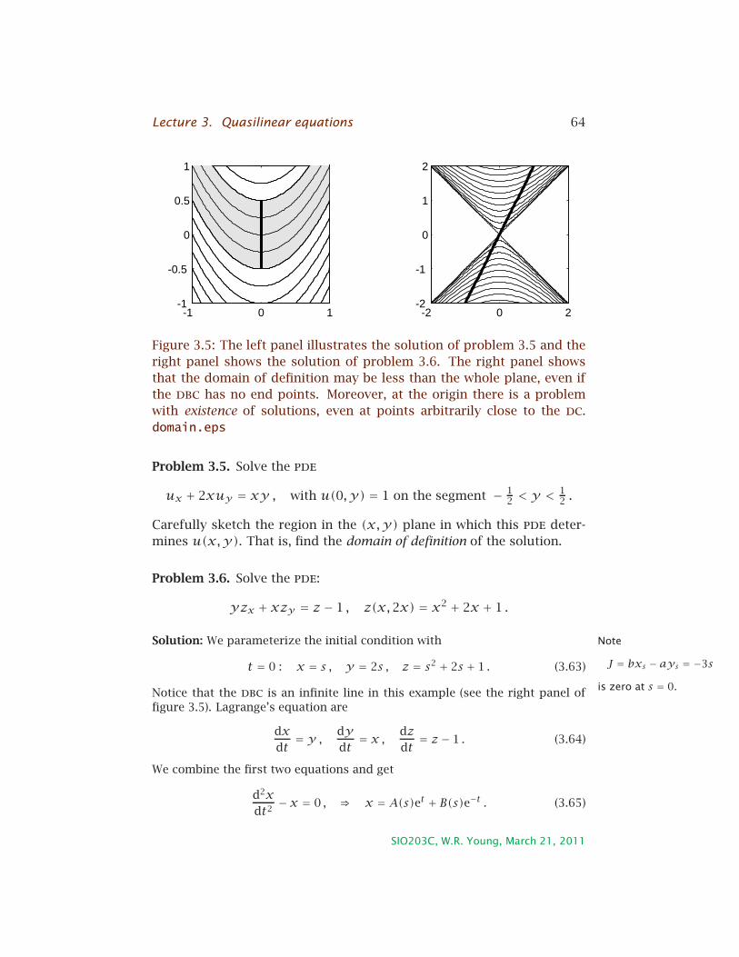
Lecture 3. Quasilinear equations 64
-1 0 1-1
-0.5
0
0.5
1
-2 0 2-2
-1
0
1
2
Figure 3.5: The left panel illustrates the solution of problem 3.5 and the
right panel shows the solution of problem 3.6. The right panel shows
that the domain of definition may be less than the whole plane, even if
the dbc has no end points. Moreover, at the origin there is a problem
with existence of solutions, even at points arbitrarily close to the dc.
domain.eps
Problem 3.5. Solve the pde
ux + 2xuy = xy , with u(0, y) = 1 on the segment − 12 < y <
12 .
Carefully sketch the region in the (x,y) plane in which this pde deter-
mines u(x,y). That is, find the domain of definition of the solution.
Problem 3.6. Solve the pde:
yzx + xzy = z − 1 , z(x,2x) = x2 + 2x + 1 .
Solution: We parameterize the initial condition with Note
J = bxs − ays = −3s
is zero at s = 0.
t = 0 : x = s , y = 2s , z = s2 + 2s + 1 . (3.63)
Notice that the dbc is an infinite line in this example (see the right panel of
figure 3.5). Lagrange’s equation are
dx
dt= y , dy
dt= x , dz
dt= z − 1 . (3.64)
We combine the first two equations and get
d2x
dt2− x = 0 , ⇒ x = A(s)et + B(s)e−t . (3.65)
SIO203C, W.R. Young, March 21, 2011

Lecture 3. Quasilinear equations 65
Also
y = dx
dt= A(s)et − B(s)e−t . (3.66)
Now, we let t = 0 and apply the initial condition in (3.63):
s = A+ B , 2s = A− B , ⇒ A = 3
2s B = 1
2s . (3.67)
Thus, we now have
x(s, t) = 3
2set − 1
2se−t , y(s, t) = 3
2set + 1
2se−t . (3.68)
The cbc’s obtained from (3.68) are plotted in the right panel of figure 3.5.
Notice that none of the cbcs enter the region in which |y| < |x|. The domain
of definition of this problem is the other region, |y| > |x|, which is ventilated
by the cbcs which pass through y = 2x.
We solve the third equation in (3.64) for z
dz
dt= z − 1 , ⇒ z = 1+ C(s)et . (3.69)
The initial condition in (3.63) now determines C(s) in (3.69):
z = 1+ s(s + 2)et . (3.70)
So much for the first two steps of the recipe.
We are now on the home stretch — we eliminate s and t in favor of x and
y . If we add and subtract the expressions in (3.68) we get
y + x = 3set , y − x = se−t . (3.71)
Multiplying the equations above together and taking a square root we get
s = +√
13(y
2 − x2) . (3.72)
(Why do we take the positive branch of the square root?) Dividing the equa-
tions (3.71) and taking another square root we get
et =√
y + x3(y − x) . (3.73)
Armed with (3.72) and (3.73) we can express z in (3.70) in terms of x and y :
z(x,y) = 1+ 13(x +y)
[2+
√13(y
2 − x2)
], byu. (3.74)
The final step is to check that the expression above solves the pde
SIO203C, W.R. Young, March 21, 2011

Lecture 3. Quasilinear equations 66
Problem 3.7. Show that the solution of
(x +u)ux +yuy = u+y2 , u(x,1) = x , −∞ < x <∞ ,
is
u(x,y) = x −y2
1+ lny+y2 .
What is the domain of definition of u(x,y)?
Problem 3.8. Solve
xux +yuuy = −xy , u(x,y) = 5 on xy = 1 .
Problem 3.9. Solve
yux + x3uy = x3y , u(x,x2) = x4 .
Problem 3.10. Show that the solution of
x3ux = uy , u(x,0) = 1
1+ x2,
is
u(x,y) = 1− 2x2y
1+ x2 − 2x2y.
Show that the solution is not defined in y > 1/2x2 even though the data
is prescribed for −∞ < x <∞.
Problem 3.11. Show that the initial value problem
(y − x)ux − (y + x)uy = 0 , u(x,0) = f(x) , x > 0 ,
has no solution if f(x) is an arbitrary function.
Problem 3.12. Consider the initial-value problems:
ux −uy = u , u(x,−x + x2) = ex ,
ux −uy = u , u(x,−x + x2) = 1 .
If the solution exists, find it and the domain of existence. If there is no
solution, explain why.
Problem 3.13. Show that the initial value problem
yux + xuy = pu u(x,x) = f(x) ,
has no solution unless f(x) = axp . If f has this form, find the solution.
SIO203C, W.R. Young, March 21, 2011

Lecture 3. Quasilinear equations 67
Problem 3.14. (i) Find a solution analogous to (3.48) of the pde
ut + c(u)ux = 0 , u(x,0) = F(x) .
(ii) Check your answer by substitution. (iii) Considering the special case
c = u2 and F = x, show that once t > 0 there are either two real values
of u(x, t) or no real values of u(x, t) at each point in spacetime. Locate
the curve in the (x, t) plane which separates these two behaviours.
Problem 3.15. (i) Find an implicit solution, analogous to (3.48), of
ut +uux = −αu , u(x,0) = 1
1+ x2.
Make sure your answer reduces to (3.48) if α → 0. Draw a figure, like
3.3, showing both characteristics and snapshots of u(x, t). (Use several
values of α so that you understand how this parameter changes the
solution). (ii) Calculate ts as a function of α. (iii) Find the smallest value
of the damping α which is sufficient to prevent shock formation.
Problem 3.16. (i) Does the pde
ut +uux = 0 , u(x,0) = ex
1+ ex.
form a shock? If so, calculate ts without solving the pde. (ii) Find an
implicit solution for u(x, t) and use matlab to graph this solution.
Solution. The geometric construction described following (3.51) makes
it clear that this initial condition does not form a shock. (Also notice
that the initial slope, ux(x,0), is positive everywhere and so according
to (3.58) the shock time, ts, is in the past.) In part (ii), we quickly find
ξ = x − eξ
1+ eξt u = eξ
1+ eξ.
Fiddling about with the second equation above, we can express ξ as an
explicit function of u: ξ = ln[u/(u − 1)]. Next, we can eliminate ξ and
give an equation which defines u implicitly as a function of x and t:
ln
(u
u− 1
)= x −ut .
We can’t solve this monster for u(x, t) explicitly. But to graph u(x, t),just as in the right panel of figure 3.3, we don’t need to...
SIO203C, W.R. Young, March 21, 2011

Lecture 3. Quasilinear equations 68
Problem 3.17. (i) Does the pde
ut +uux = 0 , u(x,0) = e−x
1+ e−x.
form a shock? If so, calculate ts without solving the pde. (ii) Find an
implicit solution for u(x, t) and use matlab to graph this solution.
Problem 3.18. In the witchy example we showed in (3.60) and (3.61) that
the time at which the shock forms is ts = 8√
3/9. Find the location, xs,
at which the shock forms.
Problem 3.19. Find an expression for ts, analogous to (3.58), for the pde
ut +u2ux = 0 , u(x,0) = F(x) .
Also give a simple formula for xs.
Problem 3.20. Consider
ut +u3ux = 0 , u(x,0) = sinx .
At what time, ts, and location, xs, does the solution u(x, t) first become
singular?
SIO203C, W.R. Young, March 21, 2011

Lecture 4
δ-functions and Green’s
functions
Can I assume that you understand the concept of a Green’s function, and
δ-functions, at least as far as odes are concerned? The material in this
lecture is in section 1.5 of BO, but here is a little review in case you need
it. In this lecture we’ll only discuss ordinary differential equations, and
we’ll begin with evolution problems in which the independent variable Notation:
θ = dθ
dt
is t = time. In this context the function δ(t) embodies the concept of
impulsive action. For example, when a hammer pounds a nail into a
plank it must exert a force on the head of the nail. If you can draw a
graph of this force as function of time then you have a good idea of
what δ(t) means.
4.1 Review of “patching"
Before we discuss δ-functions we review the solution of ordinary differ-
ential equations with discontinuous coefficients and forcing functions.
This is the method of “patching”. We illustrate patching by solving a few
simple examples from mechanics.
The poster child of discontinuous functions is Oliver Heaviside’s step
function
H(t) =
0 , if t < 0;
1 , if t > 0.(4.1)
69

Lecture 4. δ-functions and Green’s functions 70
0 0.5 10
0.2
0.4
0.6
0.8
1
t
H(t)
I1(t)
I2(t) I
3(t)
−2 −1 0 1 2
0
0.2
0.4
0.6
0.8
1
t
Hε(t)
Figure 4.1: Left panel: The step function H(t), and three successive
integrals using the definition in (4.5). The singular behavior at t = 0 is
smoothed out by integration. Right panel: the smoothed step function
Hǫ(t) defined in (4.21). In this illustration ǫ = [0.4,0.2,0.1,0.05,0.025].jumpy.eps
Notice we’ve left H(0) undefined. As we solve the following differential
equations it will become clear that the value of H(0) is irrelevant. If it
makes you feel better you can define it as H(0) = 1/2, but it makes no
difference.
Consider a differential equation involving H(t), such as the third or-
der example ...y − 7y − 6y = H(t) . (4.2)
Something on the left hand side must balance the discontinuous forcing
function on the right. Suspicion falls heavily on the term with the most
derivatives i.e.,...y in the example above. This means that at t = 0 the
third derivative...y is discontinuous:
limǫ→0
[ ...y(−ǫ)−
...y(ǫ)
]= 1 . (4.3)
The terms with fewer derivatives are better behaved i.e., y(t) is contin-
uous at t = 0. This is a general principle: Taking derivatives makes a
singularity worse. The converse is: Integrating makes a singularity bet-
ter.
Let’s beat this point to death by considering the Heaviside step H(t),
SIO203C, W.R. Young, March 21, 2011

Lecture 4. δ-functions and Green’s functions 71
0 10 20 30 40 50 600
0.5
1
1.5
2
time, t
θ(t)
Figure 4.2: The solid curve is the undamped-oscillator solution in (4.8).
With no damping, the oscillator rings around the equilibrium solution
θ = 1. The dashed curve is the solution for a lightly damped oscillator
in problem 4.4 (µ/σ = 0.1 in this illustration). oscillator.eps
and the functions obtained by successive integration
I1(t) =∫ t
−∞H(t′)dt′ , (4.4)
I2(t) =∫ t
−∞I1(t
′)dt′ , (4.5)
and so on. It is easy to see that In(t) = H(t)tn/n!. The left panel
of figure 4.1 shows that the sudden behaviour at t = 0 becomes less
prominent as we successively integrate.
Example: Solve
θ + σ 2θ = 1 , θ(0) = θ(0) = 0 .
The oscillator is at rest at t = 0 and then suddenly a constant force is
switched on. When t > 0 the general solution is
θ(t) = σ−2︸ ︷︷ ︸
=particular solution
+ A cosσt + B sinσt︸ ︷︷ ︸=homogeneous solution
.
The constants A and B are determined so that the initial conditions are
satisfied. Thus at t = 0 we require that both θ and θ are zero. Applying
these initial conditions we quickly find
θ(t) = σ−2 (1− cosσt) . (4.6)
SIO203C, W.R. Young, March 21, 2011

Lecture 4. δ-functions and Green’s functions 72
The differential equation has a steady equilibrium solution, namely θ(t) =1. But the solution we’ve found above in (4.6) “rings” forever round this
equilibrium — see Figure 4.2.
Example: Solve
θ + σ 2θ = H(t) , θ(t < 0) = 0 . (4.7)
This problem is almost equivalent to the example we just did, and the
solution is
θ(t) = σ−2 (1− cosσt) H(t) . (4.8)
This is the solid curve in Figure 4.2. The H(t) is inserted above so that
we can interpret the solution on the whole time axis −∞ < t < ∞. When
t < 0 the oscillator is at rest and minding its own business: the H(t) on
the right of (4.8) takes care of that. Then suddenly at t = 0 the oscillator
is disturbed by the application of the constant force. We insist that θ(t)and θ(t) are continuous at t. Therefore both θ and θ are zero at t = 0+,
and we immediately recover the solution in the previous example. Notice
that θ (the term with the most derivatives) jumps discontinuously:
θ(0−) = 0 , and θ(0+) = 1 .
This is perfectly OK: on the right of the differential equation (4.7) we have
the discontinuous function H(t), which is balanced by the discontinuous
function θ(t) on the left.
Example: Solve
φ+ σ 2φ = H(t)−H(t − τ) , φ(t < 0) = 0 . (4.9)
Using linearity and temporal translation invariance, the solution is
φ(t) = θ(t)− θ(t − τ) ,
where θ(t) is defined in (4.8). One absolutely must include the H(t)in (4.8) if this beautiful trick is to work. Back in the previous example
the H(t) seems like a fussy little device. But in this example the H(t)ensures that the solution φ(0 < t < τ) does not anticipate that the
forcing on the right of (4.9) is going to switch off at the future time
t = τ.
When t > τ the solution is
φ(t > τ) = σ−2 [cosσ(t − τ) − cosσt] . (4.10)
We can pick τ so that the φ(t) above is equal to zero e.g., take στ = 2π .
Alternatively if στ = π then the oscillation has maximum amplitude
viz., φ(t > τ) = −2 cosσt. So the ultimate amplitude of the oscillation
can be nicely controlled by timing when the force is switched off
SIO203C, W.R. Young, March 21, 2011

Lecture 4. δ-functions and Green’s functions 73
4.2 δ-sequences
The δ–function is not a real function; instead, the δ–function is inter-
preted as the limit (ǫ → 0) of a sequence of functions with two proper-
ties:
(a):
∫∞
−∞δǫ(t)dt = 1;
(b): δǫ(t)→ 0 as ǫ → 0 with t ≠ 0 fixed. (4.11)
Because of property (a), the integral of each member of the sequence
is independent of the parameter ǫ. Property (b) is satisfied because the
functions become very sharply peaked as ǫ → 0. We will denote the
δ–sequence by δǫ(t) but for brevity we denote the limit (when ǫ = 0)
simply by δ(t).
There is a simple recipe for producing δ–sequences. Start with some
‘humplike’ function, h(t), which is normalized so that the integral of his equal to one. Here are some examples:
h1(t) =e−t
2
√π, h2(t) =
1
π
1
1+ t2 , h3(t) =sin t
πt. (4.12)
To obtain a δ-sequence, take
δǫ(t) =1
ǫh
(t
ǫ
). (4.13)
Make sure you understand why the construction above satisfies the prop-
erties in (4.11). (There are other recipes for obtaining a δ–sequence; the
one above is the most elementary.)
The limit of a δ-sequence is only defined when the sequence is inside
an integral. For example, if f(t) is a smooth function then
∫∞
−∞f(t1)δ(t − t1)dt1
def= limǫ→0
∫∞
−∞f(t1)δǫ(t − t1)dt1. (4.14)
Because of the integrand on the right of (4.14) is nonzero only in the
immediate neighbourhood of t1 = t, we can pull the slowly varying func-
tion f(t1) outside the integral so that:
∫∞
−∞f(t1)δ(t − t1)dt1 = f(t) . (4.15)
SIO203C, W.R. Young, March 21, 2011

Lecture 4. δ-functions and Green’s functions 74
This is the ‘sifting–property’ of a δ–function.
Here is a list of some of the more useful properties of the δ-function:
f(t)δ(t − t1) = f(t1)δ(t − t1) (4.16)
tδ(t) = 0 (4.17)
δ(−t) = δ(t) (4.18)
δ(at) = |a|−1δ(t) . (4.19)
In addition, there is the crucial sifting property in (4.15).
Integration by parts shows that the derivative of the δ-function has
the property ∫∞
−∞f(t)δ′(t)dt = −f ′(0). (4.20)
We can viewH(t) as the limit of a sequence of very smooth functions.
This limiting process is illustrated in the right panel of Figure 4.1 using
H(t) = limǫ→0
1
1+ exp(−t/ǫ)︸ ︷︷ ︸def=Hǫ(t)
. (4.21)
It is easy to see that the t-derivative of the sequence Hǫ(t) defines a
perfectly good δ-sequence:
δǫ(t) =dHǫdt
. (4.22)
Thus blithely saying ‘the derivative of the limit is the limit of the deriva-
tive’, we get
d
dtH(t) = δ(t) . (4.23)
This is an extremely useful result, and it reinforces our earlier point that
differentiating a singular function makes the singularity worse — δ(t) is
more singular than H(t).
Example: Suppose we build a δ-function using the recipe in (4.13) and the
asymmetric hump function:
h4(t) =e−t
2
√π(1+αt) .
Is (4.18) satisfied, even though h4(t) ≠ h4(−t) ?
SIO203C, W.R. Young, March 21, 2011

Lecture 4. δ-functions and Green’s functions 75
Yes: (4.18) means that if f (t) is any function which is continuous at
t = 0 then
limǫ→0
∫∞
−∞f (t)
1
ǫh4
(t
ǫ
)dt = lim
ǫ→0
∫∞
−∞f (t)
1
ǫh4
(−tǫ
)dt .
The result above is correct because the symmetry-breaking term propor-
tional to α in h4(t) gives a vanishing contribution in the limit.
Example Although tδ(t) = 0, tδ′(t) ≠ 0. Show that tδ′(t) = −δ(t).
sgn(t) = 1+H(t)2
If a function is discontinuous at a point, its derivative at that point
is a δ-function with an amplitude that is proportional to the size of the
discontinuity. Equation (4.23) is one example, and another is the func-
tion sgn(t) which is equal to ±1 according to whether x is positive of
negative. Thusd
dtsgn(t) = 2δ(t) . (4.24)
This is not mysterious. If a < 0 < b then, on one hand, a pedestrian
application of the definition of sgn(t) gives:
∫ b
asgn(t)
df
dtdt =
∫ b
0
df
dtdt −
∫ 0
a
df
dtdt (4.25)
= f(b)− 2f(0)+ f(a) . (4.26)
On the other hand, we can use (4.23) to integrate by parts:
∫ b
asgn(t)
df
dtdt = [sgn(t)f (t)]ba −
∫ b
a2δ(t)f(t)dt ,
= f(b)− 2f(0)+ f(a) . (4.27)
Although we’ve differentiated a discontinuous function, everything is
hunky dory.
4.3 Green’s function of the harmonic oscillator
The idea of a Green’s function is illustrated by the following example.
Suppose we need to solve the forced oscillator equation
θ + σ2θ = f(t) , θ(0) = θ(0) = 0 . (4.28)
SIO203C, W.R. Young, March 21, 2011

Lecture 4. δ-functions and Green’s functions 76
Although this problem is posed as an initial value problem beginning at
t = 0, we can also think of it as posed on −∞ < t <∞ provided we agree
that
f(t < 0) = 0 and θ(t < 0) = 0 . (4.29)
That is, nothing is happening when t < 0, and then the force f(t)switches on at t = 0 and sets the oscillator into motion.
Suppose we somehow first solve the equation
G + σ2G = δ(t) , G(t < 0) = 0 . (4.30)
Then the solution of (4.28) is
θ(t) =∫∞
−∞G(t − t′)f(t′)dt′ . (4.31)
The function G(t) is called the Green’s function, or sometimes the funda-
mental solution, of (4.28). The Greens function is the oscillation induced
by a δ-function kick. It is a remarkable fact that if we can solve the
differential equation with this kick-forcing, then we can solve the equa-
tion with any forcing f(t) via the formula (4.31). In the next section we
discuss this concept for a general class of linear systems.
Noting1 that G(t) and f(t) are both zero when t < 0, we can re-write
(4.31) as
θ(t) =∫ t
0G(t − t′)f(t′)dt′ . (4.32)
This seems simpler than (4.31). However the limits ±∞ in (4.31) are
convenient when we prove that (4.31) satisfies (4.28) by substitution:
(d2
dt2+ σ2
)θ(t) =
∫∞
−∞
(d2
dt2+σ2
)G(t − t′)f(t′)dt′ ,
=∫∞
−∞δ(t − t′)f(t′)dt′ ,
= f(t) . (4.33)
Notice we used time-translation symmetry above: if G(t) is the response
to a kick at t = 0, then G(t − t′) is the response to a kick at t = t′.This is all very well, but we still have to solve (4.30). We begin by
noting that the forcing term on the right hand side is zero except in
1We’ve used causality: G(t) is the response of an oscillator to an impulsive kick.
The oscillator is at rest before its kicked i.e., G(t < 0) = 0.
SIO203C, W.R. Young, March 21, 2011

Lecture 4. δ-functions and Green’s functions 77
the neighborhood of t = 0. Thus the solution when t < 0 is simply
G(t) = 0. Then, at t = 0, the oscillator gets an impulsive kick from the
δ-function. The effect of the kick is calculated by integrating (4.30) over
a small time interval that surrounds t = 0, say −τ < t < τ. Because
G(−τ) = G(−τ) = 0 the result of this integration is
G(τ)+ σ2
∫ τ
−τG(t)dt = 1. (4.34)
As τ → 0 one of the terms on the left hand side must balance the 1
on the right hand side. Some thought shows that it must be G(τ) since
the other term vanishes as τ → 0. This means there is a jump in G at
t = 0: G(t) is continuous, G(t) is discontinuous at t = 0 and G(t) has a
δ-function component at t = 0. Notation: 0+is 0 plus a
bit, and 0− is 0 minus a
bit.To summarize this argument: the effect of δ-function function forc-
ing on the right hand side of (4.30) is to produce a jump in G(t) at t = 0:
G(0−) = G(0+) = 0, G(0−) = 0, G(0+) = 1. (4.35)
The conditions at t = 0+ can then be used as “effective initial conditions”
for the homogeneous equation G +σ2G = 0, and the solution is
G(t) = σ−1 sin(σt)H(t) . (4.36)
The factor H(t) is inserted to remind us that the oscillator is at rest
when t < 0.
The expression in (4.31) gives the unfortunate impression that the
θ(t) =∫∞
−∞G(t−t′)f (t′)dt′
solution at time t depends on what happens in the future: the integral
involves knowing f(t′) with t′ > t. Now that we have the Green’s func-
tion in (4.36) we see that2
θ(t) =∫ t
−∞σ−1 sin
[σ(t − t′)
]f(t′)dt′ . (4.37)
If the forcing is zero when t < 0 then we can also replace the lower
limit above by zero, so the integral runs from 0 to t. However we might
consider a slightly more general problem in which
limt→−∞
f(t) = 0 , and limt→−∞
θ(t) = 0 . (4.38)
2The same solution is found by variation of parameters. Green’s solution provides
much more physical insight.
SIO203C, W.R. Young, March 21, 2011

Lecture 4. δ-functions and Green’s functions 78
The expression in (4.37) is the solution of this problem in which the
oscillator is at rest in the distant past.
Once again, the general principle is that higher derivatives of a func-
tion become increasingly singular: in an equation like (4.30) it is always
the most highly differentiated term (in this case G) that balances the
δ-function:
G = δ(t) as t → 0. (4.39)
The δ-function cannot be balanced by G, since then G would be a δ-
function derivative, and G would be a double derivative of δ, and there
is nothing to balance this horrible singularity.
Notice also that the bare mathematical problem
G + σ2G = δ(t) , (4.40)
has the solution in (4.36), but also at least two other solutions
G2 = −σ−1 sin(σt)H(−t) and G3 = 12σ
−1 sinσ |t| . (4.41)
All the G’s above a have a derivative-jump at t = 0: G(0+) − G(0−) = 1.
We have made specific use of causality to identify (4.36) as the relevant
Green’s function. We’ll see later that the solutions above might (and in
fact do) appear in other physical problems.
Example: Find an integral representation of the causal solution of
...y − 7y − 6y = f (t) .
The forcing f (t) is zero when t < 0, and so is y(t). Find a condition on
f (t) which ensures that limt→∞y(t) < ∞.
The causal Green’s function satisfies
...g − 7g − 6g = δ(t) , g(t < 0) = 0 .
“Causal” means nothing happens before the kick arrives at t = 0 i.e.,
g(t < 0) = 0. When t > 0 the general solution of the homogeneous
equation is obtained with g = eλt , leading to
λ3 − 7λ− 6 = 0 or λ = −1, −2 and +3.
The cubic polynomial for λ above is solved by inspired guessing, or with
the mathematica command
Roots[x^3 - 7 x + 6 == 0, x]
SIO203C, W.R. Young, March 21, 2011

Lecture 4. δ-functions and Green’s functions 79
Thus the general solution when t > 0 is
g = ae−t + be−2t + ce3t . (4.42)
We have to determine the constants a, b and c by applying initial condi-
tion at t = 0+, just after the impulse. At t = 0 the δ-kick is balanced by...y , so integrating from t = −ǫ to t = +ǫ we have
g(ǫ)− g(−ǫ)︸ ︷︷ ︸=0
=∫ ǫ
−ǫδ(t)dt
︸ ︷︷ ︸=1
In other words, the second derivative g jumps discontinuously from zero
to one as a result of the kick. The function g(t) and the first derivative
g(t) are continuous at t = 0, implying that g(0) and g(0) are zero. Thus
we have three effective initial conditions
g(0+) = 0 , g(0+) = 0 , g(0+) = 1 (4.43)
to determine the three constant a, b and c in (4.42). The conditions
above result in the 3× 3 linear system
a+ b + c = 0 ,
a+ 2b − 3c = 0 ,
a+ 4b + 9c = 1 .
Solving the equations above we find
g =[−1
4e−t + 15e−2t + 1
20e3t]H(t) , (4.44)
where the H(t) is inserted for causality. The general causal solution is
therefore
y(t) =∫ t
0g(t − t′)f (t′)dt′ .
The long-time behaviour of y(t) will be dominated by the term in g(t)proportional to e3t :
y(t) = e3t
20
∫ t
0e−3t′f (t′)dt′ + decaying terms e−t and e−2t .
To completely destroy the growing term as t → ∞ one requires that the
forcing satisfy
limt→∞
e3t
∫∞
0e−3t′f (t′)dt′ = 0 .
The advantage of the Green’s function is that one can obtain general re-
sults determining important qualitative properties of the solution, such
as the condition above. If one wants to solve the equation with a partic-
ular f (t) then it may be best to avoid the Green’s function integral repre-
sentation and use simpler techniques such as undetermined coefficients
SIO203C, W.R. Young, March 21, 2011

Lecture 4. δ-functions and Green’s functions 80
Example: Find an integral representation of the solution of...h − 7h− 6h = δ(t) .
satisfying limt→±∞h(t) = 0.
This problem is different from the previous one because we don’t seek
a causal solution i.e., we might have h(t < 0) ≠ 0. Instead we’re after a
solution on the whole t-axis, −∞ < t < ∞, which is zero as t → −∞ and
as t → +∞.
Lets work out the details. The homogeneous problem is the same as the
previous case, and the conditions at ±∞ demand
h(t) =pe3t , for t < 0;
qe−t + re−2t , for t > 0.(4.45)
The construction above secures the vanishing of h(t) as t → ±∞. Now
the three constants of integration are determined by patching at t = 0
i.e., by requiring that h and h are continuous at t = 0, and that h(0+)−h(0−) = 1. Thus
p = q + r ,3p = −q − 2r ,
q + 4r − 9p = 1 .
Solving the equations above, we find we can write the solution as
h(t) = g(t)− 120e3t ,
where g(t) is the causal solution back in (4.44). With hindsight this is
obvious: the difference g(t)− h(t) satisfies the homogeneous equation,
and we construct h(t) from g(t) simply by subtracting the t → +∞growing component e3t
4.4 The black box
I have introduced the concept of the Green’s function as the impulse-
response of the oscillator equation in (4.30). However the idea is much
more general and important than this example might suggest. Suppose
we have a device (the legendary ‘black box’) that accepts an input U(t)and produces an output V(t). We don’t enquire about the internal work-
ings of the black box. Obviously this is a very general concept e.g., one
can view ones colleagues as black boxes.
Some black boxes are simpler than others. The very simplest exam-
ples are:
SIO203C, W.R. Young, March 21, 2011

Lecture 4. δ-functions and Green’s functions 81
Black boxU(t) V(t)
Figure 4.3: The black box with input U(t) and output V(t).BlackBox.eps
1 Causal; the black box can’t anticipate future events.
2 Time translationally invariant; if the input U(t) produces V(t),then U(t − t1) produces V(t − t1).
3 Linear; the response to αU1(t)+α2U2(t) is αV1(t)+α2V2(t).
An example of this type of simple black box is a simple thermometer.
The input to a thermometer might be the “true temperature” of the air
surrounding the bulb; the output is the “measured temperature”. If the
true temperature is changing rapidly (for instance, if the thermometer
is mounted on the wing of a plane) then the measured temperature will
be some smoothed or averaged or “filtered” version version of the true
temperature.
Another example is the measured deflection V(t) of a structure at
some point in response to a varying load U(t) at some other point. If
the load is not too great then we expect that the response varies linearly
with the load. Buildings don’t start shaking before an earthquake, so the
system is causal. And if the material in the structure isn’t aging then the
response to a standard load now and six months from now will be the
same. These are the three requirements above.
The three assumptions are sufficient to completely characterize the
operation of the black box if we know the response produced by the spe-
cial input δ(t). This is the impulse response, or the Green’s function of
the black box, denoted by G(t). Given G(t), the response to an arbitrary
input U(t) is
V(t) =∫ t
−∞G(t − t′)U(t′)dt′. (4.46)
Thus, if we measure or calculate the response of the black box to a single
SIO203C, W.R. Young, March 21, 2011

Lecture 4. δ-functions and Green’s functions 82
−2 0 2 40
0.2
0.4
0.6
0.8
1
time, t
V(t
) an
d U
(t)
V(t)U(t)
Figure 4.4: The input is H(t) and output V(t) ramps up over a time τ to
the final level (τ = 2 in this illustration). ramp.eps
input, δ(t), then we know how the system responds to any input by
evaluating the integral in (4.46).
Because the response V(t) cannot depend on the future behaviour of
the input U(t), the upper limit of integration in (4.46) is t′ = t. (Anyway,
because G(t < 0) = 0 you can write +∞ as the upper limit if you like —
it won’t make any difference.)
To prove (4.46), partition up the t-axis into small intervals of length
dt and then approximate the input U(t) as a ‘staircase’, with a constant
value in each dt-interval. The response to each ‘pulse’ in the staircase is
then given by a single Green’s function (multiplied by dt) and (4.46) is
the result of linearly superposing these responses.
Example: Suppose that the input temperature is H(t) and the observed re-
sponse to this step function input is
V(t) =
0 , if t < 0;
t/τ , if 0 < t < τ;
1 , if τ < t.
This ramp is shown in Figure 4.4. Find the Green’s function. The con-
stant τ is a response time of the thermometer.
The Green’s function of the thermometer is obtained by using (4.23) i.e.,d
dtH(t) = δ(t)by taking the derivative of the step–response V(t) in Figure 4.4:
G(t) = τ−1 [H(t)−H(t − τ)] . (4.47)
We’ve used linearity to say that if the input U(t) elicits the response
V(t), then the response to dU/dt is dV/dt.
SIO203C, W.R. Young, March 21, 2011

Lecture 4. δ-functions and Green’s functions 83
Now using (4.46) and (4.47) we can write down a simple expression for
the response of this hypothetical thermometer to any input:
V(t) = 1
τ
∫ t
t−τU(t′)dt′ . (4.48)
We see that the thermometer is averaging the arriving signal U(t) over
the most recent times. The averaging is done ‘on–the–fly’, so that the
measurement at t depends on the past temperature back to t − τ
Example: Find the response of the thermometer to a signal u(t) = eiωt . Dis-
cuss the two limitsωτ ≫ 1 and ωτ ≪ 1.
Example: Suppose two of these thermometers are connected in series so that
the input of the second is the output is the first. Find the response of
this composite system to the inputs δ(t) and H(t).
4.5 Problems
In example 1 of section 7.4, BO give short shrift to the elementary but im-
portant method of patching. Their discussion of δ-functions and Green’s
function in section 1.5 is a little more complete, but still not very de-
tailed. The first six or seven problems are examples of “patching".
Problem 4.1. Use patching to obtain non-trivial solutions of the differ-
ential equations
y ′ + sgn(x)y = 0 , y(±∞) = 0 ,
y ′′ + sgn(x)y = 0 , y(−∞) = 0 .
Problem 4.2. Solve
y ′′′ +y = H(x) , y(−∞) = 0 , y(∞) = 1 .
(Above, H(x) is the Heaviside step function.)
Problem 4.3. Consider the oscillator problem
χ + σ2χ = tτH(t)−
(t
τ− 1
)H(t − τ)
︸ ︷︷ ︸def= r(t)
, χ(t < 0) = 0 .
Draw a graph of the right hand side r(t) as a function of t. Solve the
initial value problem and discuss how the amplitude of the ultimate os-
cillation depends on τ.
SIO203C, W.R. Young, March 21, 2011

Lecture 4. δ-functions and Green’s functions 84
Problem 4.4. (a) Solve the forced-damped oscillator problem
θ + µθ + σ2θ = H(t) , θ(t < 0) = 0 .
Check your answer by comparing it with the dashed curve in Figure 4.2.
(b) Show that as t → ∞ half the work done by the force H(t) is used
to increase the potential energy of the oscillator and the other half is
dissipated by drag.
Problem 4.5. Solve
θ + σ2θ = 0 , θ(t < 0) = a cos(σ1t +α) ,
where
σ2(t) =
σ2
1 , if t < 0;
σ22 , if t > 0.
Problem 4.6. Solve the forced oscillator equation
θ + θ = e−α|t| , limt→−∞
θ(t) = 0 .
Check your answer by showing that the amplitude of the oscillation at
t = +∞ is maximized by taking α = 1.
Problem 4.7. Reconsider the forced oscillator problem in the example
surrounding (4.9). Obtain the Green’s function in (4.36) by taking the
limit τ → 0 of the solution in (4.10).
Problem 4.8. (i) Show that
f(n, z) =√n
∫∞
−∞
dx
[1+ (x − z)2]n
is independent of z and becomes independent of n in the limit n → ∞.
(A heuristic argument based on the size of the interval in which the
integrand is significantly different from zero is all that is required.) (ii)
Use the well known result(
1+ yn
)n→ ey as n→∞
to evaluate f(∞, z). (iii) Approximately evaluate the integral
I ≡∫∞
0
cosx2
(1+ x2)4dx.
SIO203C, W.R. Young, March 21, 2011

Lecture 4. δ-functions and Green’s functions 85
Problem 4.9. Evaluate
I ≡ limǫ→0
∫∞
−∞
ǫ sin (ex)
ǫ2 + x2dx .
and
J = limǫ→0
∫∞
−∞sin (ex)
d
dx
ǫ
ǫ2 + x2dx .
Problem 4.10. Make a δ–sequence with the function sech2(x).
Problem 4.11. Explain why the dimension of δ(t), with t=time, is (time)−1.
In general δ-functions are dimensional quantities (unlike bona fide func-
tions such as cosωt).
Problem 4.12. Use integration by parts to evaluate∫ 1−1 |t|f ′′(t)dt. (Don’t
be afraid to differentiate |t| twice.)
Problem 4.13. (i) Show that if f(x) is a function which vanishes at xnthen
δ[f(x)] =∑
n
δ(x − xn)|f ′(xn)|
. (4.49)
(ii) Calculate ∫∞
−∞δ(sinx) exp(−|x|)dx . (4.50)
(iii) Show that
δ(t2 − a2
)= [δ(t − a)+ δ(t + a)] /2|a| . (4.51)
Problem 4.14. If (x,y) = r(cosθ, sinθ), show that
∮δ(a− x cosφ−y sinφ)dφ = 2H(r − a)√
r2 − a2. (4.52)
Problem 4.15. Verify by substitution that (4.37) satisfies (4.28).
Problem 4.16. Consider the pendulum in the strongly over-damped limit.
After suitable scaling the equation of motion is
µθ + θ + θ = f(t) ,
where µ ≪ 1. Obtain the Green’s function G(t) for this problem. Since
µ ≪ 1 one might be tempted to neglect the term µθ. Make this approx-
imation and obtain the Green’s function of the approximate equation.
Use matlab to make a graphical comparison between the two Green’s
functions µ = 0.01 and 0.1.
SIO203C, W.R. Young, March 21, 2011

Lecture 4. δ-functions and Green’s functions 86
-2 0 2 4 6 8
0
0.5
1
x
A a
nd d
A/d
x
Functions A(x) and dA/dx
Figure 4.5: Figure for Problem 4.20. When x < 0 the two curves coincide.
Problem 4.17. Suppose that the output of our hypothetical thermometer
is observed to be:
V(t) =
0 , if t < 0;
= 1− exp(−αt) , if t > 0.
Reconstruct the input, U(t). (This one might be tough.)
Problem 4.18. Find the impulse response of a linear system in which the
output V(t) is obtained from from the input U(t) by solving
V + 2V + V = U .
Problem 4.19. Find the Green’s function of the equation
dny
dtn= f(t) , with lim
t→−∞y(t) = 0 .
(Assume that f(t) vanishes at least exponentially fast as t → −∞.) Con-
sider the function Y(t) defined by
(d
dt
)17
Y = e−t2
cosmt , with limt→−∞
Y(t) = 0 .
Show that when t≫ 1
Y(t) ∼ A(m)t16 +O(t15
),
and find A(m).
SIO203C, W.R. Young, March 21, 2011

Lecture 4. δ-functions and Green’s functions 87
Problem 4.20. The figure above shows a function A(x) and its derivative
dA/dx. Here are some differential equations:
B′′′ + B = H , C′′ − C = −H , D′′′ −D = −H .
H(x) on the RHS is the Heaviside step function, which is zero if x < 0
and one if x > 0. (i) Which of the differential equations does A(x)satisfy? (Guesses don’t count — explain your reasoning.) (ii) Sketch a
graph of A′′(x), paying particular attention to the behaviour of A′′ near
x = 0.
SIO203C, W.R. Young, March 21, 2011
Lecture 5
Green’s functions for boundary
value problems
5.1 A suspended string
In our earlier examples of Green’s functions and δ–functions the inde-
pendent variable is time. The examples we discussed were evolution-
ary problems and consequently we frequently made arguments using
causality and stationarity. But there is another equally important class
of models based on the impulses or point singularities in the spatial do-
main. As an example of a spatial Green’s function, consider the wave
equation 1
ρutt − Tuxx = −ρg, u(0) = u(L) = 0 . (5.1)
The tension in the string is T (same dimensions as force), and ρ is the
mass per unit length of the string; the boundary conditions are that the
ends of the string are fixed at x = 0 and x = L. The right hand side
of (1) is a force per length which, in a gravitational field, is simply the
weight of the string. If the string has nonuniform thickness then ρ is a
function of x.
Example: Find the steady (ut = 0) solution of (1) when ρ is a constant.
Example: Consider a string with uniform density ρ0. A small bead of massmis then attached to the middle (x = L/2) of the string. Use a δ-function
1We’ll discuss the wave equation in much more detail later. The material in this
section can be understood without reference to this important physical example.
88

Lecture 5. Green’s functions for boundary value problems 89
to represent the total mass density, ρ(x) of the composite system. Find
the steady (ut = 0) solution of (1) for this composite system and sketch
the shape of the string whenm≫ ρ0L.
Our goal is to find an integral representation of the steady solution,
ut = 0, of (1) when ρ is some given function of x. After suitable non-
dimensionalization, the problem is
y ′′ =w(x), y(0) = y(1) = 0, (5.2)
where w ∝ ρ is a prescribed function of x. The ends of the string at
x = 0 and x = 1 are fixed so that that there is no displacement. Unlike
the oscillator equation, this is a boundary value problem; the indepen-
dent variable, x, is a spatial variable (not time); there is no principle of
causality here. A second difference is that the problem is not transla-
tionally invariant: the point x = 1/4 is not the same as x = 1/2 because
x = 1/2 is maximally distant from the supports at x = 0 and x = 1.
Thus, for instance, if we load the string with a point mass then the dis-
placement at x = 1/4 is less than the displacement at x = 1/2.
To solve (5.2) we first must solve for the displacement produced by
an impulse load at an arbitrary point on the string. Thus, the Green’s
G′ = dG
dxfunction, G(x, ξ), satisfies
G′′ = δ(x − ξ), G(0) = G(1) = 0. (5.3)
If we integrate (5.3) over a small interval containing the δ function then
we obtain the jump condition at x = ξ:
G′(ξ+)−G′(ξ−) = 1. (5.4)
G itself is continuous at x = ξ. Next, we consider the interval 0 < x < ξand write down the most general solution of Gxx = 0 which satisfies the
boundary condition, namely, G(x) = Ax. We do the same in the interval
ξ < x < 1. Thus, in this second interval, G = B(1− x).Enforcing continuity of G at ξ and the jump condition in (4) gives
Aξ = B(1− ξ), and − B −A = 1 . (5.5)
Solving for A and B, we finally have the Green’s function:
G(x, ξ) =
−(1− ξ)x , if 0 < x < ξ;
−(1− x)ξ , if ξ < x < 1.(5.6)
SIO203C, W.R. Young, March 21, 2011

Lecture 5. Green’s functions for boundary value problems 90
Now that we have the Green’s function, the solution of (5.2) is obtained
by linear superposition
y(x) =∫ 1
0G(x, ξ)w(ξ)dξ (5.7)
You can check that (5.7) satisfies (5.2) by substitution; you’ll need to use
the sifting property of the δ-function.
The Green’s function above is not a function only of x − ξ because
the problem is not translationally invariant. However there is a certain
symmetry between x and ξ. If you draw the contours of constant G in
the (x, ξ) plane you will see that the function is unchanged if you reflect
in the line x = ξ. In terms of algebra, this symmetry means that
G(x, ξ) = G(ξ,x). (5.8)
This is the principle of reciprocity.
Example: Suppose that the boundary conditions in are inhomogeneous
yxx = w(x), y(0) = 0, y(1) = 1.
(For example, one end of the string is clamped at a higher level than the
other.) Find an integral representation for the solution of this problem.
If we represent the solution as y(x) = x + y(x), then y(x) satisfies
the problem with homogeneous boundary conditions. Thus the general
solution is
y(x) = x +∫ 1
0G(x, ξ)w(ξ)dξ ,
where G(x, ξ) is the Green’s function in (5.6).
5.2 Solvability conditions
Now suppose that both ends of the string are ‘free’. This means that the
boundary conditions of (2) are changed so that
y ′′ = w(x), y ′(0) = y ′(1) = 0. (5.9)
Proceeding as before, we hope to obtain the Green’s function by solving
G′′ = δ(x − ξ), G′(0) = G′(1) = 0. (5.10)
SIO203C, W.R. Young, March 21, 2011

Lecture 5. Green’s functions for boundary value problems 91
However, when we try solve (5.10), it all goes horribly wrong: there is no
solution.
With hindsight we see that if we integrate (5.9) from x = 0 to x = 1
we find that 0 =∫ 10 w(x)dx; this is a contradiction unless the integral of
w happens to be zero. Thus, generally, (5.9) does not have a solution. So
the problem is not with our Green’s function technique — we are trying
to solve a problem without a solution, and the method tells us this very
quickly. You cannot ask for more than this from mathematics alone.
Returning to the physical problem back in (5.1) makes the source of
our difficulties clear. The string is in a gravitational field, but the ends
are unsupported. Thus the string falls freely. The string does remain
stretched between x = 0 and x = L; the ends can push and pull in the
horizontal direction, but they cannot exert a vertical force — this is what
I mean by ‘free’. (You can imagine some configuration of curtain rings
and slippery vertical rods etcetera.)
In fact, if we integrate (5.1) from x = 0 to x = L, with free boundary
conditions ux = 0, then we obtain
∫ L
0ρutt dx =
∫ L
0ρg dx. (5.11)
Thus the problem does not have a steady solution. This is where all our
difficulties spring from: we assumed a steady solution and none exists.
Here is the cure: if the string starts from rest then the solution of (5.11)
is that
u = 1
2gt2, u(t) ≡
∫ L
0ρudx
/∫ L
0ρg dx; (5.12)
u(t) is the mass weighted average of the displacement (that is, the verti-
cal position of the center of gravity of the string). So now we look at the
displacement relative to this falling level
u′(x, t) ≡ u(x, t)− u(t). (5.13)
Substituting (5.13) into (5.1) we find that u′ satisfies (1) with the right
hand side replaced by zero. This result is expected because u′ is the
displacement in a freely falling frame of reference (in which there is no
apparent gravity).
Now return to the mathematical problem in (5.9) and suppose that it
does happen that ∫ 1
0w(x)dx = 0. (5.14)
SIO203C, W.R. Young, March 21, 2011

Lecture 5. Green’s functions for boundary value problems 92
If w does satisfy this ‘solvability condition’ then we do not obtain a
contradiction when we integrate (8) from x = 0 to x = 1 and we opti-
mistically guess that the differential equation does have a solution. Let
us now find an integral representation of this solution. The correct mod-
ification of (5.10) is that
G′′ = δ(x − ξ)− 1, G′(0) = G′(1) = 0. (5.15)
The solution of (14) where x ≠ ξ is that
G(x, ξ) =
−1
2x2 +A , if 0 < x < ξ;
−12x
2 + x + B if ξ < x < 1.(5.16)
This construction satisfies the boundary conditions at x = 0 and x = 1.
Now we hope to determine the constants A and B from the jump condi-
tions at x = ξ. One of these conditions is that G(x, ξ) is continuous at
x = ξ, so that
A = ξ + B. (5.17)
The other condition, obtained by integrating across the δ–function is
that
G′(ξ+, ξ)−G′(ξ−, ξ) = 1 . (5.18)
But when we apply this condition we discover that it is automatically
satisfied by the solution in (5.16). Thus we have only one condition,
namely (5.17), to determine the two constants A and B. So the most
general solution of (14) is that
G(x, ξ) = A+
−1
2x2 − ξ , if 0 < x < ξ;
−12x
2 + x − ξ , if ξ < x < 1.(5.19)
Above, A is any constant. This seems strange, but the arbitrary constant
A is expected because now, in retrospect, it is obvious that if y(x) is a
solution of (5.9) then so is y(x) + A. The Green’s function is telling us
that the original boundary value problem has an infinite number of solu-
tions. This example gives you a glimpse of the problems which are pre-
sented by inhomogeneous boundary value problems: sometimes there
is no solution and other times there are an infinite number of solutions!
SIO203C, W.R. Young, March 21, 2011

Lecture 5. Green’s functions for boundary value problems 93
5.3 Problems
Problem 5.1. Find the Green’s function of the boundary value problem
y ′′ = w(x), y(0) = 0, y ′(1) = 0 .
Give a simple formula for y ′(0) in terms of w(x).
Problem 5.2. Find the Green’s function of
y ′′ −y = f(x); y(±∞) = 0.
Problem 5.3. Find a Green’s function representation of the solution of
the inhomogeneous boundary value problem
[xd
dx
]2
y −y = f(x), y(1) = y(∞) = 0 .
Problem 5.4. Consider the boundary value problem
y ′′ =w(x) , with y(0) = 0 and y ′(1) = αy(1);
the boundary condition at x = 1 is ‘mixed’. Find the Green’s function
and show that there is a particular value of α for which the problem has
no solution for an arbitrary w(x). Considering this exceptional case,
find the “solvability condition" — the analog of (5.14) — which ensures
that the problem does have a solution and then obtain the appropriate
Green’s function.
Problem 5.5. Find solutions of the differential equations
y ′′′ +y = δ(x) ,[
d2
dx2− 1
]2
y = δ′(x) ,
which vanish at x = ±∞. In both cases give an explicit real expression
for y(0). In both cases calculate
∫∞
−∞y(x)dx , and
∫∞
−∞xy(x)dx .
(Look for a way to evaluate the integrals without having to explicitly
solve the equation.)
SIO203C, W.R. Young, March 21, 2011

Lecture 6
The diffusion equation
ut = κ∇2u
6.1 Origin of the diffusion equation
The equation governing heat diffusion in a solid is
cut = ∇∇∇···(k∇∇∇u) (6.1)
where u(xxx, t) is the temperature. Also in (6.1), where is the density
of the solid (kilograms per cubic meter), c the heat capacity (Joules per
kilogram per Kelvin) and k the conductivity (find the units yourself). This
is in the form of a conservation law
∂t[energy density
]+∇∇∇···
[energy flux
]= 0 . (6.2)
The flux is fff = −k∇∇∇u, so if the temperature is uniform then there is no
flux of energy. In the 17th century, people thought of heat as “caloric
fluid” that flows down the temperature gradient, from hot regions to
colder regions. This caloric theory has been superseded by thermody-
namics, but I think it still provides some useful intuition.
Notice that if we integrate (6.2) over a closed volume V , with surface
∂V , then with Gauss’s theorem we have
d
dt
∫
Vcudv
︸ ︷︷ ︸energy in V
=∫
∂Vk∇∇∇u···nnnds ,
︸ ︷︷ ︸energy flow through the surface ∂V
(6.3)
94

Lecture 6. The diffusion equation ut = κ∇2u 95
where nnn is the unit outward normal to the surface of ∂V . This is the
multi-dimensional analog of an integral conservation law.
If all three of the three material properties ρ, c and k are constant
we can bundle them into one combination,
κ ≡ k
c, (6.4)
called the diffusivity. Then the simplest form of the diffusion equation
is
ut = κ∇2u . (6.5)
Random walkers
Another context in which the diffusion equation arises is the random
walk. In the one-dimensional case, u(x, t) is the density (walkers per
meter) and f = −κux is the flux (walkers per second). In this example
κ = (mean square step length)2
2× average time between steps. (6.6)
Let’s sketch the random walk model and explain how it produces the
diffusion equation.
We begin with the classical model in which the random walk is dis-
crete in both space and time. The walker (traditionally a drunk) takes a
step at times t = τ, 2τ, · · · . The steps are ±a with probability 1/2. We
consider an ensemble of walkers and let ρ(x, t) be the number of walk-
ers at site x at time t. It is easy to see that the evolution of the ensemble
of walkers is given by
ρ(t, x) = 12ρ(t − τ,x −a)+
12ρ(t − τ,x + a) . (6.7)
i.e. half of the walkers at site x−a hop to the right and land at x and so
on. Equation (6.7) is a partial difference equation i.e., a discrete system
with two independent variables. With an initial condition, such as
ρ(x,0) = δ(x) , (6.8)
it is easy to iterate a few times and find ρ(x, τ), ρ(x,2τ) etc. You might
like to do this and see if you can guess the general result (hint: Pascal’s
triangle).
SIO203C, W.R. Young, March 21, 2011

Lecture 6. The diffusion equation ut = κ∇2u 96
We can obtain the diffusion equation (6.5) as an approximation to
(6.7) when ρ(x, t) is slowly changing i.e., when the spatial variation of
ρ is on a scale much larger than the hopping length a, so that in one
iteration from t to t + τ there is only a small change in ρ(x, t). This
“macroscopic evolution equation” follows easily from (6.7) if we rewrite
it as
ρ(t, x)−ρ(t−τ,x) = 12 [ρ(t − τ,x − a)− 2ρ(t − τ,x)+ ρ(t − τ,x + a)] .
(6.9)
Now we make the slowly varying assumption: we expand everything in
sight in the small parameters a and τ: Small relative to what?
ρ(t − τ,x) = ρ(t, x)− τρt(t, x)+O(τ2) , (6.10)
and Take τ = O(a2) and
neglect O(τ2)
ρ(t−τ,x±a) = ρ(t, x)−τρt(t, x)±aρx(t, x)+ 12a
2ρxx(t, x)+O(a3) .(6.11)
Putting all this into (6.9) and isolating the surviving term on each side
we get
ρt = κρxx (6.12)
where
κ ≡ a2
2τ. (6.13)
Why do we keep the O(a2) terms in (6.11), and neglect the O(τ2)terms in (6.10)? This seems inconsistent. Neglect of the O(τ2) terms
can be justified by taking a distinguished limit in which a→ 0 and τ → 0
with ratio κ in (6.13) fixed; with this procedure τ and a2 have the same
order. In taking this limit we suppose that instead of (6.8) we have a
smooth initial condition containing a length scale ℓ:
ρ(x,0) = f(x
ℓ
), (6.14)
and that ℓ is fixed as a and τ go to zero with κ fixed. In this limit, the
term τρtt — and all the other higher-order terms such as a4ρxxxx —
disappear.
SIO203C, W.R. Young, March 21, 2011

Lecture 6. The diffusion equation ut = κ∇2u 97
6.2 Smoothing a discontinuity or “front”
Considering the problem
ut = κuxx , u(x,0) = A sgn(x) , (6.15)
we quickly see that the only dimensionally consistent form for the solu-
tion is
u(x, t) = A× some function of x/√κt . (6.16)
Thus we are inspired to try the guess ξt = −ξ/2t
u(x, t) = AU(ξ) , ξ ≡ x/√κt . (6.17)
We start calculating
U ′ ≡ dU
dξux =
A√κtU ′ , uxx =
A
κtU ′′ , ut = −
A
2tξU ′ (6.18)
and substitute into the pde:
− A2tξU ′ = κ A
κtU ′′ ⇒ −ξU ′ = 2U ′′ . (6.19)
Our efforts are crowned with success when all the t’s cancel and we are
left with the boxed ode for U(ξ).
Now we solve that ode using separation of variables. Integrating
twice
U ′ = C1e−ξ2/4 , U(ξ) = C1
∫ ξ
0e−v
2/4 dv + C2 . (6.20)
The constants C1 and C2 are determined by insisting that
limξ→±∞
U(ξ) = ±1 , (6.21)
or:∫∞
0e−v
2/4 dv =√π− 1 = −
√πC1 + C2 , 1 =
√πC1 + C2 , ⇒ C1 =
1√π, C2 = 0 .
(6.22)
Thus we now have
U(ξ) = 1√π
∫ ξ
0e−v
2/4 dv . (6.23)
Adjusting our notation, we rewrite the solution in (6.23) as
u(x, t) = Aerf(η) , (6.24)
SIO203C, W.R. Young, March 21, 2011

Lecture 6. The diffusion equation ut = κ∇2u 98
-2 -1.5 -1 -0.5 0 0.5 1 1.5 2-1
-0.5
0
0.5
1erf(η)
η
Figure 6.1: The function erf(η). erfPic.eps
where the similarity variable is now
erf(z) ≡ 2√π
∫ z
0e−u
2duη ≡ x
2√κt. (6.25)
The erf function is shown in figure 6.1.
6.3 Discussion of the similarity method
This similarity method is a powerful technique for solving or simplifying
both linear and nonlinear pde’s. Above I have also demonstrated the
powerful educational technique of glossing quickly over the profound
part of the method — the guess in (6.17) — and dwelling at length on
algebraic technicalities.
To explain the similarity method in more detail suppose that Tom
and Jerry are both struggling with (6.15). Tom is measuring length in
meters and seconds, but Jerry is an engineer and prefers to use furlongs
and fortnights. Tom uses x and t to denote space and time and Jerry
uses x′ and t′. The numerical values of these coordinates can be con-
verted one to the other by
x′ = λx , t′ = µt . (6.26)
It follows that Tom and Jerry’s numerical values for the diffusivity are
related by κ′ = λ2κ/µ.
Even before Tom & Jerry solve the pde they realize that the solution
must satisfy
u = AF(x, t, κ) = AF(λx︸︷︷︸x′
, µt︸︷︷︸t′
, λ2κ/µ︸ ︷︷ ︸κ′
) . (6.27)
SIO203C, W.R. Young, March 21, 2011

Lecture 6. The diffusion equation ut = κ∇2u 99
All that we have done is assume the existence of a formula which gives
u once either set of variables is specified. The essential point is that this
is the same formula no matter which set of units is used. Then as we
freely vary both λ and µ the value of u at the same point in space-time is
unchanged i.e., (6.27) is always true for all values of µ and λ. This implies
that x, t and κ appear in F only in the combination x2/(κt) = x′2/(κ′t′)— that’s where we started back in (6.17).
One difficulty with the argument above is that the initial condition
can never be totally discontinuous. Suppose the initial condition is really
something like
u(x,0) = A tanh(x/ℓ) = A tanh(x′/ℓ′) . (6.28)
i.e., some smooth function which changes from−A to +A over a distance
ℓ′ = µℓ. As soon as Tom and Jerry admit the existence of this length
they must also amend (6.27) to
u = AF(x, t, κ, ℓ) = AF(λx,µt, µκ/λ2, λℓ) . (6.29)
Now as one freely varies λ and µ the most that one can deduce is that
u = AF(x/ℓ, κt/ℓ2) = AF(x′/ℓ′, κ′t′/ℓ′2) . (6.30)
This is a useful result because it tells us that we can economically present
the solution using a function of two (rather than four) variables. But
there is no longer a similarity solution.
On the other hand, it seems reasonable that if we consider a sequence
of problems with smaller and smaller ℓ’s then in the limit we should
approach the sgn(x) initial condition and the erf similarity solution. Al-
ternatively, with fixed ℓ, once the diffusively spreading front becomes
much thicker than ℓ then ℓ is an “irrelvant” parameter. In this case wet≫ ℓ2/κget the erf solution as the asymptotic description of a diffusing front.
This possibility is consistent with (6.29) if
(p, q)→ ∞ ⇒ F(p, q)→ F(p/√q) . (6.31)
6.4 The Green’s function for diffusion on the line
To solve the initial value problem
ut = κuxx , u(x,0) = f(x) , (6.32)
SIO203C, W.R. Young, March 21, 2011

Lecture 6. The diffusion equation ut = κ∇2u 100
we need the Green’s function, which is defined by
gt = κgxx , g(x,0) = δ(x) . (6.33)
Once we possess g(x, t) it is easy to see by substitution that
u(x, t) =∫∞
−∞f(x′)g(x − x′, t)dx′ (6.34)
is the solution of (6.32). To find g(x, t) we use the erf-solution as the
thin end of the wedge: since
δ(x) = 12
d
dxsgn(x) , (6.35)
the Green’s function of the diffusion equation is
g(x, t) = 12
∂
∂xerf(η) ,
= e−x2/4κt
√4πκt
. byu (6.36)
Another derivation of the diffusion Green’s function
An alternative route to (6.36) is to argue on dimensional grounds that
g(x, t) = 1√κtG
(x√κt
). (6.37)
As an exercise you should substitute this guess into the diffusion equa-
tion and recover (6.36) by solving the resulting ode.
Where does the factor 1/√κt on the rhs of (6.37) come from? Ap-
parently
dim(g) = length−1 . (6.38)
Because of the initial condition in (6.33) the dimensions of g are the
same as the dimensions of δ(x). Now δ-functions have the peculiar
property that
dim [δ(θ)] = 1
dim(θ). (6.39)
That is, δ-functions have the inverse dimension of their argument. (Other
functions, such as cosx or ln t, are dimensionless.) In the problem
SIO203C, W.R. Young, March 21, 2011

Lecture 6. The diffusion equation ut = κ∇2u 101
(6.33), the argument of the δ-function is x, with dimensions of “length”,
and therefore g has dimensions (length)−1.
Another way to understand the factor 1/√κt is to observe that if we
integrate the diffusion equation from x = −∞ to x = ∞ we have:
d
dt
∫∞
−∞g(x, t)dx = [κgx(x, t)]x=∞x=−∞ = 0 . (6.40)
(We assume the solution decays quickly as x → ±∞ so that there is no
flux of g-stuff from ±∞.) Using the initial condition we deduce that
∫∞
−∞g(x, t)dx = 1 . (6.41)
Now the factor 1/√κt is just what the similarity guess in (6.37) needs in
order to the satisfy the conservation law (6.41):
1 =∫∞
−∞G
(x√κt
)dx√κt=∫∞
−∞G (ξ) dξ . (6.42)
This little argument based on conservation laws also tells us how to
determine a constant of integration which arises as we solve the ode
which results from stuffing (6.37) into the diffusion equation.
Convolution
In (6.34) we have the solution of the diffusion equation as the convolution
of the initial condition f(x) with the Green’s function g(x, t). Let us
discuss the convolution of two functions in more detail. Alternative
terms used to describe
c(x) =∫∞
−∞a(x′)b(x − x′)dx′
︸ ︷︷ ︸the convolution of a with b
=∫∞
−∞a(x −x′)b(x′)dx′
︸ ︷︷ ︸convolution is commutative
, (6.43)
are faltung, superposition integral, running mean, smoothing, scanning
and blurring.
To appreciate the origin of these terms, consider the case when b(x)in (6.43 is a “box-car filter"
b(x) =
1 , if |x| < 12 ,
0 , otherwise.(6.44)
SIO203C, W.R. Young, March 21, 2011

Lecture 6. The diffusion equation ut = κ∇2u 102
Then at every point x, c(x) is an averaged, or smoothed or low-pass fil-
tered version of version of a(x). Explaining this requires drawing some
examples, such as visually computing the convolution
c(x) =∫∞
−∞sgn(x′)b(x − x′)dx′ =
−1 , if x < −12 ,
2x , if −12 ≤ x ≤
12 ,
+1 , if12 < x.
(6.45)
The box-car filter smooths out the sudden jump at x = 0 into a ramp.
The convolution in (6.34) shows that the value of u(x, t) is deter-
mined by averaging the initial condition of f(x) over an interval of width√κt centered on the point x. The Green’s function (6.36) is a Gaussian
filter, and the range of the filter grows as√κt. Thus as t increases the
width of the averaging interval increases, and therefore u(x, t) becomes
increasingly smooth. The effect of convolving sgn(x) with the box-car is
the ramp in (6.45) and convolution of sgn(x) with the Gaussian is the erf
in Figure 6.1. The two results are qualitatively similar: the discontinuity
is smeared out over a distance comparable to the filter width.
6.5 Solution of the diffusive initial value problem
Having the general solution of the infinite-line diffusion problem in (6.34)
and (6.36) is very pleasant — particularly because the interpretation as
a convolution-average provides intuition. But be aware that (6.34) may
not be the easiest way to solve simple problems. For example, consider
the initial value problem
ut = κuxx , u(x,0) = coskx . (6.46)
Guessing that the solution is separable
u = A(t) coskx , (6.47)
we quickly find by substitution that
dA
dt= −κk2A , ⇒ u(x, t) = e−κk
2t coskx . (6.48)
If we can convince ourselves that the diffusion equation has a unique
solution, then we have shown
e−κk2t coskx︸ ︷︷ ︸
separation of variables
=∫∞
−∞coskx′
e−(x−x′)2/4κt
√4πκt
dx′ .︸ ︷︷ ︸
the Green’s function solution
(6.49)
SIO203C, W.R. Young, March 21, 2011

Lecture 6. The diffusion equation ut = κ∇2u 103
Example: Solve the initial value problem
ut = κuxx , u(x,0) = e−m2x2
. (6.50)
We can guess that if we release a suitably scaled δ-pulse at t0 < 0 then at
t = 0 this pulse will have evolved into the Gaussian above. So consider
ut = κuxx , u(x, t0) = Aδ(x) , (6.51)
with solution
u = Ae−x2/4κ(t−t0)
√4πκ(t − t0)
. (6.52)
Evaluating this at t = 0 we obtain t0 = −1/(4m2κ), and we also deter-
mine the amplitude A. The final answer is
u(x, t) = e−m2x2/(1+4m2κt)
√1+ 4m2κt
(6.53)
Example: Solve the initial value problem
ut = κuxx , u(x,0) = xe−m2x2
. (6.54)
If u is a solution of the diffusion equation, then so is ux . So, noting that
the initial condition in this example is
xe−m2x2 = − 1
2m2
d
dxe−m
2x2
, (6.55)
we can employ the solution of the previous example to conclude that
u(x, t) = − 1
2m2
d
dx
e−m2x2/(1+4m2κt)
√1+ 4m2κt
= xe−m2x2/(1+4m2κt)
(1+ 4m2κt)3/2 (6.56)
New solutions from old
In the examples above we’ve used some quasi-obvious properties of the
diffusion equation to manufacture new solutions from old solutions.
Just to be clear, let’s summarize all these tricks. The most important
observation is that the diffusion equation is linear: if u1 and u2 are
solutions then so is an arbitrary linear combination a1u1 + a2u2.
Moreover, if u(x, t) is a solution of the diffusion equation then:
1. so is u(−x, t), and so is u(x + x0, t + t0) where x0 and t0 are
arbitrary constants;
SIO203C, W.R. Young, March 21, 2011
Lecture 6. The diffusion equation ut = κ∇2u 104
2. so is ∂mx u(x, t), and so is ∂nt u(x, t);
3. so is u(αx,α2t), where α is an arbitrary constant.
Under the operations above the diffusion equation is transformed into
itself.
The transformational properties of differential equations is an im-
portant field of mathematics, initiated by Lie over a century ago. This
is not the main focus of these lectures. But just to show that Lie group
methods lead to non-obvious results, I remark that the transformation
t′ = t + c , x′ = x − 2ct − c2 , u′ = uecx−c2t−c3/3 (6.57)
transforms the diffusion equation to itself:
ut = κuxx ⇒ u′t′ = κu′x′x′ . (6.58)
There is nothing quasi-obvious about this transformation.
Uniqueness
To prove that the diffusion equation has a unique solution, suppose to
the contrary that the initial value problem
vt = κ∇2v , v(xxx,0) = f(xxx) . (6.59)
has two solutions, v1(xxx, t) and v2(xxx, t) say. Then the difference u =v1−v2 also satisfies the diffusion equation, but with the initial condition
u(xxx,0) = 0 . (6.60)
Now let’s proceed assuming that u might be non-zero and show that
this leads to a contradiction. Multiply the diffusion equation by u and
shuffle the result into the following form
12
(u2)t= κ∇∇∇2
(u2)− κ|∇∇∇u|2 . (6.61)
Notice that although u satisfies a conservation equation, u2-stuff is not
conserved: u2 is destroyed at a rate κ|∇∇∇u|2. Integrating over the entire
space1 we have
12
d
dt
∫u2 dV = −κ
∫|∇∇∇u|2 dV . (6.62)
1OK — there is an assumption of rapid decay at infinity so that∫u∇∇∇u···nnndA can be
dismissed. In finite domain with homogeneous BCs there is no assumption necessary.
SIO203C, W.R. Young, March 21, 2011

Lecture 6. The diffusion equation ut = κ∇2u 105
Now integrate with respect to time
12
∫u2 dV = −κ
∫ t
0
∫|∇∇∇u|2 dV dt ; (6.63)
This is a contradiction: the left is positive and the right is negative.
The moment method
Even when guessing doesn’t work, one can still extract very useful infor-
mation about the solution without actually solving the diffusion equa-
tion.
Suppose, for example, that the initial condition in (6.32) is a hump,
such as f(x) = sechx. We can use (6.34) and write down an integral rep-
resentation of the solution immediately. But if we are content with less
than total information we can get a good qualitative feel by considering
the moments of the solution:
mp(t) =∫∞
−∞xpu(x, t)dx . (6.64)
If we think of u(x, t) as a density then m0 is the total mass and
X(t) ≡ m1
m0(6.65)
is the center of mass. The variance or moment of inertia is
σ2 ≡m−10
∫∞
−∞(x −X)2u(x, t)dx = (m2/m0)−X2 . (6.66)
If we know m0, X and σ then we know how much stuff there is, where
the stuff is, and how far its spread out.
Multiplying (6.32) by xp, with p = 0, 1 and 2, and integrating from
x = −∞ to x = ∞ we see
m0 = 0 , m1 = 0 , m2 = 2κm0 . (6.67)
The proof is integration by parts; the key intermediate step is
∫∞
−∞x2uxx dx = [x2ux − 2xu]∞−∞︸ ︷︷ ︸
=0
+2
∫∞
−∞udx
︸ ︷︷ ︸=2m0
. (6.68)
SIO203C, W.R. Young, March 21, 2011

Lecture 6. The diffusion equation ut = κ∇2u 106
Substituting (6.67) into (6.65) and (6.66) we find that both m0 and X are
constant while
σ2 = σ20 + 2κt . (6.69)
Thus diffusion leaves the mass and the center of mass fixed but in-
creases the width of the hump linearly with time. This gives us a good
qualitative picture for the evolution of an initial pulse of heat.
The maximum principle
We can also show that if u(x, t) is a solution of (6.32) then the maximum
(and minimum) of u(x, t) for all x and t ≥ 0 is at t = 0. That is, the
largest possible value of u is present in the initial condition f(x).
We can deduce this maximum principle from the Green’s function
solution (6.34). This expresses u at the point (x, t) as an average of fover an interval of width
√κt centered on x. If u had a maximum at x
with t > 0, then this u would be larger than every value of f contributing
to the average. This is impossible.
Another proof is by contradiction: suppose that there is an isolated
maximum of u(x, t) at some time t > 0. Then at this point
ux = ut = 0 , and uxx < 0 . (6.70)
The conditions above are inconsistent with u(x, t) being a solution of
the diffusion equation.
6.6 Diffusion with a source
Consider the forced heat equation
ut − κuxx = s(x, t) , u(x,0) = f(x) . (6.71)
Without any loss of generality we can take f(x) = 0 — we can always
use linear superposition to add on the part of the solution due to the
initial condition.
If we knew the Green’s function
Gt − κGxx = δ(x)δ(t) (6.72)
SIO203C, W.R. Young, March 21, 2011

Lecture 6. The diffusion equation ut = κ∇2u 107
then we could instantly write the solution of (6.72) as
u(x, t) =∫∞
−∞dx′
∫∞
0dt′G(x − x′, t − t′)s(x′, t′) . (6.73)
To determine G(x, t) we integrate (6.72) from t = 0− to t = 0+:
G(x,0+)−G(x,0−)︸ ︷︷ ︸=0
−∫ 0+
0−Gxx(x, t)dt
︸ ︷︷ ︸negligible
= δ(x) , (6.74)
and conclude that
G(x,0+) = δ(x) . (6.75)
In other words, the inhomogeneous Green’s function problem is equiv-
alent to the initial value problem solved back in (6.33). Thus we have
wasted a perfectly good symbol, G, because:
G(x, t) = g(x, t) = e−x2/4κt
√4κπt
H(t) . (6.76)
We add the Heaviside factor H(t) to remind us that the Green’s function
is zero if t < 0. The Green’s function g(x, t) does double-duty: the
solution of (6.71) is
u(x, t) =∫∞
−∞f(x′)g(x−x′, t)dx′ +
∫∞
−∞dx′
∫ t
0dt′ s(x′, t′)g(x−x′, t − t′) .
(6.77)
Example: Solve the forced diffusion equation
vt = κvxx + exp(−m2x2) , v(x,0) = 0 . (6.78)
Let’s save the formula (6.77) for exercise 6.9. Instead, notice that in an
earlier example we considered the initial value problem
ut = κuxx , u(x,0) = exp(−m2x2) , (6.79)
and obtained the solution in (6.53). Now you can easily show by substi-
tution that
v(x, t) =∫ t
0u(x, t′)dt′ =
∫ t
0
e−m2x2/(1+4m2κt′)
√1+ 4m2κt′
dt′ (6.80)
SIO203C, W.R. Young, March 21, 2011

Lecture 6. The diffusion equation ut = κ∇2u 108
solves (6.78). We beat this into a standard form involving an exponential
integral with the substitution
z = m2x2
(1+ 4m2κt′), dt′ = −x
2
4κ
dz
z2; (6.81)
thus
v(x, t) = |x|4mκ
∫m2x2
m2x2
1+4m2κt
e−z
z3/2dz . (6.82)
6.7 Specialized references to diffusion
For an interesting perspective on diffusion problems see
Be Random Walks in Biology by H.C. Berg.
A classic handbook on diffusion is
CJ Conduction of Heat in Solids by H.S. Carslaw & J.C. Jaeger.
A recent book emphasizing probability theory is
Re A Guide to First-Passage Processes by S. Redner.
For similarity solutions, with lots of physical examples, see
Ba Scaling, Self-similarity, and Intermediate Asymptotics by G.I. Baren-
blatt.
For Lie group methods see
Ol Applications of Lie Groups to Differential Equations by Peter W. Olver.
Springer, 1986.
SIO203C, W.R. Young, March 21, 2011

Lecture 6. The diffusion equation ut = κ∇2u 109
-40 -30 -20 -10 0 10 20 30 40-1
0
1t=1
-40 -30 -20 -10 0 10 20 30 40-1
0
1t=4
-40 -30 -20 -10 0 10 20 30 40-1
0
1t=16
-40 -30 -20 -10 0 10 20 30 40-1
0
1t=64
-40 -30 -20 -10 0 10 20 30 40-1
0
1t=256
Figure 6.2: The solution of problem 6.2. diffutz.eps
6.8 Problems
Problem 6.1. Reconsider the hopping model in (6.7), assuming that the
drunk hops to the right with probability p and to the left with probability
q, where p + q = 1. If p > q then there is a bias towards the right.
Find a distinguished limit in which the macroscopic evolution of the
slowly varying density ρ(x, t) is determined by the advection-diffusion
equation
ρt + cρx = κρxx . (6.83)
Your answer should include expressions for c and κ in terms of τ, a, pand q.
Problem 6.2. Write a matlab program to iterate (6.7) with τ = a = 1.
The initial condition is
ρ(x,0) = sgn(x) ,
where x = [−40 : 1 : 40]. As boundary conditions take ρ(±40) = ±1.
Compare your numerical solution of the discrete system (6.7) with the
appropriate erf similarity solution at t = 1, 4, 16, 64 and 256.
SIO203C, W.R. Young, March 21, 2011

Lecture 6. The diffusion equation ut = κ∇2u 110
The most boring part of this problem is getting matlab to subplot atthe right times and in the right place. Here’s some of my code showinghow this drudgery is handled. The educational part of the problem is tofill in the ????’s.
x = [-40:1:40]; %% The discrete grid
xx = [-40:0.25:40]; %% For plotting the erf solution
u = sign(x);
n = length(u);
tplot = [1 4 64 256];
nPlot = 0;
for t=[1:1:256]
?????????
?????????
?????????
if t==4^(nPlot)
nPlot = nPlot + 1;
subplot(5,1,nPlot)
plot(x,u,’.’,’markersize’,10)
hold on
plot(xx,erf(????))
time = num2str(t)
text(-15,0.4,[’t=’time])
end
end
Problem 6.3. Obtain the Green’s function for the damped advection-
diffusion equation by solving
gt + cgx = κgxx − βg , g(x,0) = δ(x) .
Hint: transform the damped advection-diffusion equation to the plain old dif-
fusion equation and use results from the lecture.
Problem 6.4. Apply the method of moments to the initial value problem
ρt + cρx = κρxx − βρ , ρ(x,0) = ρ0(x) .
The initial condition is a compact humplike density e.g., something like
ρ0(x) = sech(x). Obtain the mass, center of mass and the width of the
hump as functions of time.
Problem 6.5. Fill in all the steps between the similarity guess (6.37) and
the solution in (6.36). Make sure you explain carefully how the similarity
ansatz is consistent with the initial condition g(x,0) = δ(x).
SIO203C, W.R. Young, March 21, 2011

Lecture 6. The diffusion equation ut = κ∇2u 111
−2.5 −2 −1.5 −1 −0.5 0 0.5 1 1.5 2 2.50
0.1
0.2
0.3
0.4
0.5
0.6
0.7
0.8
0.9
1
x
u(x
,t)
t = 0.01, 0.1, 0.5 and 1 t = 0.01, 0.1, 0.5 and 1 t = 0.01, 0.1, 0.5 and 1 t = 0.01, 0.1, 0.5 and 1
Figure 6.3: Diffusive smoothing of the initial condition in problem 6.7.
diffcompz.eps
Problem 6.6. Find a similarity solution of the nonlinear diffusion equa-
tion
ut = κ (um)xx , u(x,0) = δ(x) .
Hint: The answer is in section 51 of Landau & Lifshitz Fluid Mechanics.
Problem 6.7. Consider the diffusion equation ut = κuxx with the initial
condition
u(x, t) =
1 , if |x| < a ;
0 , otherwise .
(i) Define nondimensional variables so that (a, κ) → 1. (ii) Use linearity
and the erf-solution in (6.24)) to solve this initial value problem. (iii) Use
matlab to illustrate your solution (see figure 6.3).
Problem 6.8. Solve the forced diffusion equation
ut − κuxx = coskx , u(x,0) = 0 .
SIO203C, W.R. Young, March 21, 2011

Lecture 6. The diffusion equation ut = κ∇2u 112
Problem 6.9. (i) As an exercise in Gaussian integrals, use the formula
(6.77) to show that the solution of
ut = κuxx + h(t)me−m
2x2
√π
, u(x,0) = 0 ,
is
u(x, t) = m√π
∫ t
0
h(t′) e−m2x2/(1+4m2κ(t−t′))
√1+ 4κm2(t − t′)
dt′ .
Above, h(t) is some function of time. (ii) Consider the limit m → ∞.
Show that the heat source is h(t)δ(x), and that the temperature at the
source is
u(0, t) = 1
2√πκ
∫ t
0
h(t′)√t − t′ dt′ .
(iii) Find a heating function h(t) that makes u(0, t) independent of time.
Problem 6.10. (i) Show that the similarity guess
u(x, t) = taf(η) , η = x/2√κt
a possible solution of the problem
ut − κuxx = δ(x)qtq−1 , u(x,0) = 0 , (q > 0) ,
only if q = a + 12 . (ii) Substitute the guess into the pde and show that
f(η) satisfies the ode
f ′′ + 2ηf ′ − 4af = 0 .
(iii) Reduce the ode above to quadratures in the special case q = 1.
Problem 6.11. A function F(x,y) is said to be homogeneous of degree
n if
F(λx,λy) = λnF(x,y) ,for any constant λ. For example, F = x/y is homogeneous with n = 0.
(i) Give examples of homogeneous functions of degree n = 0, 1 and 2.
(ii) Obtain a pde satisfied by F(x,y) and solve this equation in terms of
an ‘arbitrary function’. [Hint: differentiate with respect to λ and then set
λ = 1.]
Problem 6.12. After (6.27) I said “As we freely vary both λ and µ the
value of u at the same point in space-time is unchanged i.e., (6.27) is
always true. This implies that x, t and κ appear only in the combination
x2/(κt) = x′2/(κ′t′).” Use the method of problem 6.11 to prove this
assertion.
SIO203C, W.R. Young, March 21, 2011

Lecture 6. The diffusion equation ut = κ∇2u 113
Problem 6.13. (i) Find the exponents a and b which make the similarity
guess
u(x, t) = tav(η) , η ≡ x/(νt)b
a possible solution of the dispersive wave equation
ut = νuxxx , u(x,0) = δ(x) .
(ii) Substitute the guess into the pde and find the ode satisfied by v(η).(iii) Solve the ode in terms of a special function you might find in the
appendix of BO.
Problem 6.14. Consider the pde
ut = κuxxx , u(x,0) = A sgn(x) .
What are the dimensions of κ? Construct a similarity solution analogous
to (6.17), and find the ode satisfied by U(ξ). Brownie points for solving
this ode.
Problem 6.15. Suppose you are given the solution, u(x, t), of the homo-
geneous initial value problem:
ut = uxxx , u(x,0) = e−x2.
(i) Express the solution of the forced initial value problem
vt = vxxx + e−x2, v(x,0) = 0 ,
in terms of u(x, t). (ii) Suppose that χ(t) = 1 when 0 < t < 1, and χ(t) =0 otherwise. Express the solution of the forced initial value problem
wt = wxxx + e−x2χ(t) , w(x,0) = 0 ,
in terms of v(x, t). (iii) Express the solution of the forced problem
ht = hxxx − 2xe−x2δ(t) , h(x, t < 0) = 0 ,
in terms of u.
SIO203C, W.R. Young, March 21, 2011

Lecture 7
Diffusion on a half-line and on a
finite domain
In the previous lecture we discussed diffusion on the whole line −∞ <x <∞. Now let’s turn to the simplest diffusion problem with a boundary,
namely the half-line x > 0.
7.1 Half-line problems and images
Consider the problem of drunks random walking along the half-line x >0. There is a manhole at x = 0 and so the drunks who reach x = 0
immediately disappear. This is equivalent to the diffusion problem
ut = κuxx u(x,0) = f(x) , u(0, t) = 0 , (7.1)
where the dimensions of u are drunks per meter. There is an absorption
boundary condition at x = 0.
The number of surviving drunks at time t is
S(t) =∫∞
0u(x, t)dx , (7.2)
and it follows from (7.1) that f = −κux
dS
dt= −κux(0, t) . (7.3)
114

Lecture 7. Diffusion on a half-line and on a finite domain 115
absorptionreflection
Figure 7.1: The method of images. In the left hand panel the absorption
boundary condition is enforced with a negative heat pulse at x = −ξ.
imageDiff.eps
The interpretation of the relation above is that the population decreases
because of flux into the manhole.
One way of describing the demographics of these unfortunate ran-
dom walkers is to use the histogram
P(t)dt = the number of lifetimes in the interval (t, t + dt). (7.4)
There is a simple relation between P(t) and S(t) because
S(t) = the number of lives longer than t ,
=∫∞
tP(t′)dt′ . (7.5)
The derivative of this relation is
P(t) = −dS
dt, (7.6)
and so from (7.3)
P(t) = κux(0, t) . (7.7)
Does this connection between the flux at t and the density of lifetimes
make sense to you?
The Green’s function of the initial value problem in (7.1), that is ab-
sorption Green’s function ga(x, ξ, t), is the solution of
gat = κga
xx ga(x,0) = δ(x − ξ) , ga(0, t) = 0 . (7.8)
SIO203C, W.R. Young, March 21, 2011

Lecture 7. Diffusion on a half-line and on a finite domain 116
Once we have ga, the solution of (7.1) is
u(x, t) =∫∞
0ga(x, ξ, t)f (ξ)dξ . (7.9)
This is a little more complicated than our earlier formulas because ga is
a function of x and ξ separately (not just x − ξ).
The δ-function at x = ξ in (7.8) might correspond to a bar which
closes at t = 0. All the patrons are suddenly ejected onto the street and
start wandering back and forth. The unlucky ones disappear into the
manhole at x = 0.
To solve this problem, take the δ-function at x = ξ and reflect it
in the boundary (x = 0) with a negative sign. Thus on the infinite line
the initial condition is odd and the diffusion equation preserves this
symmetry so that ga(0, ξ, t) remains zero at all times. The solution of
(7.8) can then be written down using linear superposition:
ga(x, ξ, t) = g(x − ξ, t)− g(x + ξ, t) ,
= 1√4πκt
[e−(x−ξ)
2/4κt − e−(x+ξ)2/4κt
]. (7.10)
Now we can calculate the number of survivors from the initial δ-
pulse:
erf(z) ≡ 2√π
∫ z
0e−u
2duS(t) = 1√
4πκt
[∫∞
0e−(x−ξ)
2/4κtdx −∫∞
0e−(x+ξ)
2/4κtdx
],
= 1√π
[∫∞
−ξ/√
4κte−u
2du−
∫∞
ξ/√
4κte−u
2du
],
= erf
(ξ√4κt
). (7.11)
When√
4κt≫ ξ, the erf simplifies to
S(t) ≈ ξ√πκt
. (7.12)
Thus death is certain, S(t)→ 0, but the average lifetime, The PDF of lifetimes is
P(t) = −S
and
S(0) = N
t = N−1
∫∞
0tP(t)dt = N−1
∫∞
0S(t)dt
︸ ︷︷ ︸divergent
, (7.13)
is infinite. This indicates that a small fraction of the population make
large positive excursions before encountering the absorbing boundary.
SIO203C, W.R. Young, March 21, 2011

Lecture 7. Diffusion on a half-line and on a finite domain 117
7.2 Heating the Earth
As physical examples of half-line diffusion, we consider two classic prob-
lems solved by Stokes in the nineteenth century.
Stokes’s first problem
The first problem is
ut = κuxx , u(0, t) = A cosωt . (7.14)
You can think of this as periodic heating the solid Earth (with the coor-
dinate x running downwards from the surface at x = 0).
The diffusion length (skin-depth) is
ℓ =√κ/ω . (7.15)
If we’re thinking of the annual cycle, and we use κ typical of dry soil: 1 year ≈ π × 107 s.
κ = 2× 10⁻³cm2s−1 , ω = 2π
π × 107s. (7.16)
leading to
ℓ ≈ 1meter . (7.17)
Because of linearity, the diurnal and annual cycles can be superimposed.
The diurnal heating has a penetration depth which is smaller by a factor
of√
365 than the annual cycle.
Since
cosωt = 12eiωt + 1
2e−iωt , (7.18)
we can obtain the solution with the subsitution
u(x, t) = e−iωtU(x)+ eiωtU∗(x) . (7.19)
This gives
U ′′ + iℓ−2U = 0 , U(0) = 12A , lim
x→∞U(x) = 0 . (7.20)
The standard guess U = epx results in p2 + iℓ−2 = 0, or
p = ±√−iℓ−1 = ±(1− i)q, where q ≡ 1√
2ℓ. (7.21)
SIO203C, W.R. Young, March 21, 2011

Lecture 7. Diffusion on a half-line and on a finite domain 118
To ensure decay as x → +∞ we must take p = −(1− i)q, so that
u(x, t) = Ae−qx 12
(eiqx−iωt + e−iqx+iωt
),
= Ae−qx cos(ωt − qx) . (7.22)
Notice there is a damped signal propagating downwards from the sur-
face — the phase speed is ω/q.
The phase shift relative to the surface is π at a depth
x∗ =√
2πℓ ≈ 4.4meters . (7.23)
When it is Summer at the surface, it is Winter at a depth of 4.4 meters.
The attenuation factor at this depth is
e−qx∗ = e−π ≈ 1
23. (7.24)
Stokes’s second problem
In the second problem the heating is turned on suddenly at t = 0
ut = κuxx , u(x,0) = 0 , u(0, t) = 1 . (7.25)
Dimensional analysis indicates that the solution has the form
u(x, t) = U(η) , with η ≡ x
2√κt. (7.26)
Substitution into the diffusion equation gives
U ′′ + 2ηU ′ = 0 , with U(0) = 1 , limη→∞
U(η) = 0 . (7.27)
Integrating this ode and applying the boundary conditions we have
erfc(z) ≡ 1− erf(z)
= 2√π
∫∞
ze−v
2dv
U = erfc(η) . (7.28)
The thermal signal penetrates into solid a distance√κt in time t.
SIO203C, W.R. Young, March 21, 2011

Lecture 7. Diffusion on a half-line and on a finite domain 119
Kelvin’s estimate of the age of the Earth
According to CJ, in deep mines the thermal gradient is about 1C every
25 meters. There is some geographic variation and on land the geother-
mal gradient Γ is in the range
10−2K m−1 < Γ < 5× 10⁻²K m−1 .
These numbers refer to non-Volcanic regions, and the differences result
from variations in the thermal diffusivity of rocks.
Let’s follow Kelvin and use the solution of Stokes’s second problem to
estimate the age of the Earth. Assume that we start at t = 0 with molten
rock at a temperature u0 = 1200K, and that this rock cools because the
surface at x = 0 is held at u = 0. This is a slight modification of Stokes’s
second problem, and the solution is
u(x, t) = u0 erf
(x
2√κt
), ⇒ ux(0, t) =
u0√πκt
. (7.29)
The elapsed time is expressed in terms of the surface gradient as
t = u20
u2xπκ
. (7.30)
Kelvin took a diffusivity for “average rock” of about 1.18× 10⁻⁶m2 s−1.
Using the smallest geothermal gradient from (7.2) , this gives for the age
of the Earth1
t ∼ 123× 106years . (7.31)
Note that√κt ∼ 68 kilometers, so that we can ignore the sphericity of
the Earth — after 123 million years the heat is still being extracted from
a thin surface layer.
The age of the Earth is closer to 4.5 billion years and the usual ex-
planation for Kelvin’s gross underestimate is that Kelvin was unaware of
radioactive heating. However Richter (1985) shows that inclusion of ra-
dioactive heating does not substantially increase estimates based on the
diffusion equation. Richter argues that it is mantle convection, which
1According to CJ, Kelvin’s opinion was that the Earth could be no older than 24
million years. Kelvin used ux = 35K per kilometer, typical of measurements near
Edinburgh. In any event, whether it is 123 million years or 24 million years, this
estimate is far too short to be consistent with the geologic record. For an amusing
account of the age of the Earth, see A Short History of Nearly Everything by Bill Bryson.
SIO203C, W.R. Young, March 21, 2011

Lecture 7. Diffusion on a half-line and on a finite domain 120
efficiently mixes the entire heat of the Earth up to the surface, that ex-
plains how the geothermal gradient can still be larger as 10 degrees per
kilometer after 4.5 billion years.
7.3 Inhomogeneous boundary conditions
How to solve
ut = κuxx , u(0, t) = u0(t) , u(x,0) = 0? (7.32)
This mathematical problem corresponds to an isothermal solid medium
occupying the half-space x > 0. At t = 0 the boundary temperature at
x = 0 is prescribed to be u0(t). This thermal forcing diffuses into the
interior, and we seek the interior temperature distribution u(x, t).
We previously considered the special case u0(t) = H(t) and obtained
the erfc similarity solution, which we write here as
u(x, t) = erfc(η)H(t) . (7.33)
The Heaviside function ensures that u(x, t < 0) = 0 i.e., there is no
disturbance before the steady surface heating switches on at t = 0.
Now consider “top-hat” forcing that switches on at t = 0 with an
amplitude τ−1, and then switches off at t = 0. We can represent this
forcing function as
u0(t) =H(t)−H(t − τ)
τ. (7.34)
We’ve taken the amplitude of the boundary forcing to be τ−1, so that as
we take the limit τ → 0 we obtain a δ(t). We can use linear superposi-
tion, and the solution in (7.33), to solve the diffusion equation with the
boundary temperature in (7.34):
u(x, t) = H(t)erfc(η)−H(t − τ)erfc(η′)τ
, (7.35)
where η′ = x/√
4κ(t − τ). The solution is shown in Figure 7.2.
Taking τ → 0 the top-hat in (7.34) becomes a δ(t+). The solution
(7.35) in this same limit τ → 0 is:
η(x, t−τ) ≈ η(x, t)−τηt(x,
SIO203C, W.R. Young, March 21, 2011

Lecture 7. Diffusion on a half-line and on a finite domain 121
0 1 2 3-1
-0.8
-0.6
-0.4
-0.2
0
0.2
0.4
0.6
0.8
1
x
u(x,
1.1)
τ=1 and t=1
0
1
2
0
1
2
0
0.1
0.2
0.3
0.4
0.5
0.6
0.7
0.8
0.9
1
x t
Figure 7.2: The solution in (7.35) with τ = κ = 1. The left panel shows
the subtraction of the two erfc’s. The right panel shows the solution
surface above the (x, t)-plane (again with τ = 1). halfDiff.eps
SIO203C, W.R. Young, March 21, 2011

Lecture 7. Diffusion on a half-line and on a finite domain 122
G(x, t) = −ηt2√πe−η
2 = x
2√πκt3
e−x2/4κt . (7.36)
This is the Green’s function for the inhomogenous half-line problem.
The solution of (7.32) is therefore:
u(x, t) =∫ t
0u0(t − t′)G(x, t′)dt′ . (7.37)
The philosophy behind this method is that we approximate the forcing
q(t) arbitrarily closely by a sequence of narrow top-hats. We know the
response to a single top-hat so we use linear superposition to write the
response to the sequence — that’s the guts of (7.37) and every other
Green’s function formula in these last few lectures.
7.4 Diffusion of a heat around a wire loop
Consider a loop of very thin wire. We suppose that the length L of the
loop is much greater than the thickness of the wire, so that heat conduc-
tion in loop is governed by the one-dimensional diffusion equation2
uT = κuXX , u(X,0) = f(X) . (7.38)
The coordinate 0 < X < L runs around the loop. The shape of the loop
is unimportant: it might be a circle or a square. What is important is
that the point x = 0 is the same as the point x = L, and the solution is
periodic with period L
u(x, t) = u(x + L, t) .
We can crack problems like this using Fourier series. To use the tools
we’ve developed so far, we first change the coordinate so that the prob-
lem is posed on the fundamental interval (−π,π) This is accomplished
with the change of variable
x = π 2X − LL
, t = κ(
2π
L
)2
T . (7.39)
2A more detailed description would require solving the three-dimensional diffusion
equation. But since the thickness of the wire is small, the temperature rapidly becomes
uniform in the transverse (y and z) directions. We’re interested in the slower process
of heat diffusion around the loop.
SIO203C, W.R. Young, March 21, 2011

Lecture 7. Diffusion on a half-line and on a finite domain 123
-2 0 2
-1
-0.5
0
0.5
1
-0.5 0 0.5
-1
-0.5
0
0.5
1
Figure 7.3: Solution of ut = uxx with the initial condition u(x,0) =sqr(x). The initial square wave is represented approximately taking 20
terms in (??). The solution is shown at t = 0.001, 0.01, 0.1 and 0.5.
Diffusion instantly smooths the discontinuity at x = 0 and x = π so
that the Gibbs oscillations disappear. sqrDiff.eps
As X goes from 0 to L, x runs from −π to π . On this fundamental
interval, the diffusion problem is
ut = uxx , u(x,0) = f(x) , (7.40)
with the periodicity condition
u(x, t) = u(x + 2π, t) . (7.41)
It is easy to see that the Fourier series
u(x, t) = a0 +n∑
k=1
e−k2t (ak coskx + bk sinkx) (7.42)
SIO203C, W.R. Young, March 21, 2011

Lecture 7. Diffusion on a half-line and on a finite domain 124
solves the diffusion equation, and satisfies the periodicity condition. To
satisfy the initial condition we use the previous results to determine
the constants ak and bk above. For example, if the initial condition
is f(x) = sqr(x) then from (??) we can immediately write down the
solution
u(x, t) = 4
π
n∑
k=1
sin[(2k+ 1)x]
2k+ 1e−(2k+1)2t . (7.43)
This solution, using 20 terms in the series (7.43), is shown in figure
7.3. We remarked previously that the Fourier series for sqr(x) converges
slowly because smooth sinusoids struggle to approximate the disconti-
nuities. However diffusion immediately blurs the initial discontinuities
into nice smooth erf’s. Once this happens the Fourier series converges
very quickly indeed: with t > 0 the coefficients in (7.43) decrease expo-
nentially with k. Consequently, as you can see in Figure 7.3, the Gibbs
oscillation disappears very quickly.
Solution of other pdes on a loop
Let’s consider other loopy pdes defined on −π < x < π : we identify
x = −π with x = +π and look for periodic solutions
u(x, t) = u(x +π, t) . (7.44)
Some examples are
ut + cux , ut = βuxxx , ut = −νuxxxx . (7.45)
We suppose that these pdes come equipped with an initial conditions,
u(x,0) = f(x) =∞∑
n=−∞fneinx . (7.46)
Because the coefficients in (7.45) are constant, it is easy to see that
the solution for each complex sinusoid in the sum has the form
u(x, t) = einx−iωt . (7.47)
In the three examples in (7.45), the “dispersion relation" is
ω = cn , ω = βn3 , ω = −iνn4 . (7.48)
SIO203C, W.R. Young, March 21, 2011

Lecture 7. Diffusion on a half-line and on a finite domain 125
The expressions above show that to solve the pde there has to be a con-
nection between the frequency ω and the wavenumber n i.e., the fre-
quency is a function of the wavenumber. Once we have the dispersion
relation, the solution of the pde with the initial condition in (7.46) is
simply
u(x, t) =∞∑
n=−∞fneinx−iωt . (7.49)
Example Solve ut = βuxxx on the loop −π ≤ x ≤ π with the initial condition
u(x,0) = eγ cosx . (7.50)
Let’s use a complex Fourier series to represent the initial condition. The
coefficients in this series are
fn =∫ π
−πe−inx+γ cosx dx
2π= In(γ) , (7.51)
where In is the modified Bessel function. Thus the solution of the pde is
u(x, t) =∞∑
n=−∞In(γ)e
i(nx−βn3t) ,
= I0(γ)+ 2
∞∑
n=1
In(γ) cos(nx − βn3t
). (7.52)
We’ve used In(γ) = I−n(γ) to write the series in terms of cosines. The
solution is shown in Figure 7.4.
% Solution of the dispersive wave equation on a loop
beta=1; gamma = 8; X = linspace(-pi,pi,100); T = [0:0.01:1];
N=40; % truncation of the Fourier series
udata = zeros(length(T),length(X));
nloop = 0;
for tt = T
nloop = nloop + 1;
u = besseli(0,gamma)*ones(1,length(X));
for n = 1:N
u = u + 2*besseli(n,gamma)*cos(n*X - beta*n^3*tt);
end
udata(nloop,:)=u;
end
waterfall(X,T,udata), xlabel(’x’), ylabel(’t’)
colormap([0 0 0]), axis([-pi pi 0 max(T) ]), grid off
set( gca,’ztick’,[-0.1*exp(-gamma) exp(gamma)] )
view(-60,15), pbaspect([ 1 1 0.75])
SIO203C, W.R. Young, March 21, 2011
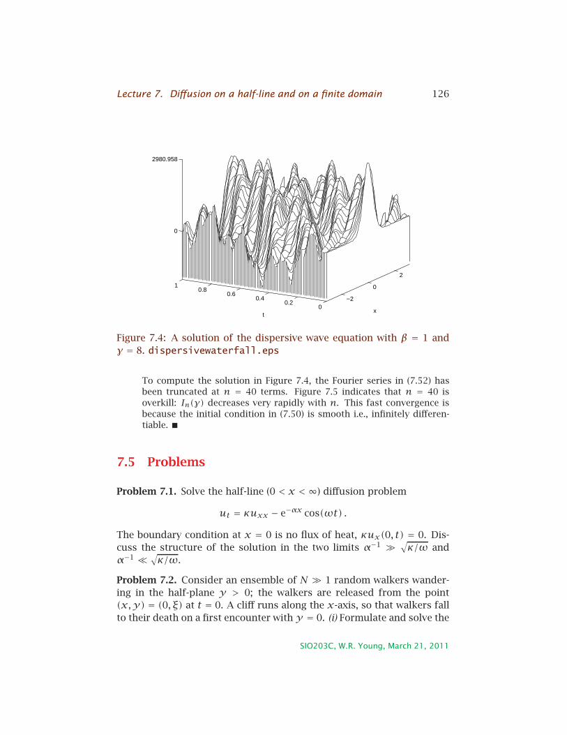
Lecture 7. Diffusion on a half-line and on a finite domain 126
−2
0
2
00.2
0.40.6
0.81
0
2980.958
xt
Figure 7.4: A solution of the dispersive wave equation with β = 1 and
γ = 8. dispersivewaterfall.eps
To compute the solution in Figure 7.4, the Fourier series in (7.52) has
been truncated at n = 40 terms. Figure 7.5 indicates that n = 40 is
overkill: In(γ) decreases very rapidly with n. This fast convergence is
because the initial condition in (7.50) is smooth i.e., infinitely differen-
tiable.
7.5 Problems
Problem 7.1. Solve the half-line (0 < x <∞) diffusion problem
ut = κuxx − e−αx cos(ωt) .
The boundary condition at x = 0 is no flux of heat, κux(0, t) = 0. Dis-
cuss the structure of the solution in the two limits α−1 ≫√κ/ω and
α−1 ≪√κ/ω.
Problem 7.2. Consider an ensemble of N ≫ 1 random walkers wander-
ing in the half-plane y > 0; the walkers are released from the point
(x,y) = (0, ξ) at t = 0. A cliff runs along the x-axis, so that walkers fall
to their death on a first encounter with y = 0. (i) Formulate and solve the
SIO203C, W.R. Young, March 21, 2011

Lecture 7. Diffusion on a half-line and on a finite domain 127
0 10 20 30 4010
−25
10−20
10−15
10−10
10−5
100
105
n
I n(γ)
γ=[1:1:10]
γ=1
γ=10
Figure 7.5: With In(γ) as a function of n at fixed values of γ between
1 and 10. This shows that coefficients of the Fourier series in (7.52)
decrease very quickly with n i.e., the series converges very quickly. To
better estimate the rate of convergence you can apply the saddle point
method to analyze the integral in (7.51) for n≫ 1 (see BO section 6.6).
besselconverge.eps
SIO203C, W.R. Young, March 21, 2011

Lecture 7. Diffusion on a half-line and on a finite domain 128
two-dimensional random walk model. (ii) Calculate the survival function
analogous to (7.2). (iii) How does the number of corpses at the foot of
the cliff vary with x as t →∞?
Problem 7.3. Solve the pde
ut + cux = κuxx , u(0, t) = cosωt ,
on the half-line x > 0. There is a nondimensional parameter, p ≡c/√ωκ. Discuss the structure of the solution in the limits c → ∞ and
c → −∞. Can you obtain these limiting solutions more simply from the
original pde by neglecting the diffusive term and solving the resulting
first-order (in x) problem?
To assist grading and discussion of this problem let us agree to use
the following notation
ν ≡ |c|2κ, λ ≡ 4
p2= 4ωκ
c2.
The identity
√1+ iλ = ±
√r + 1
2+ i
√r − 1
2
, r ≡
√1+ λ2
(which applies only if λ > 0) might also be useful. If you use the identity,
then prove or verify it and explain what happens if λ < 0.
Problem 7.4. (i) Find the reflection Green’s function
grt = κgr
xx gr(x,0) = δ(x − ξ) , grx(0, t) = 0 ,
using the method of images. (ii) The center of mass of the pulse is
X(ξ, t) ≡∫∞0 xg
r(x, ξ, t)dx∫∞0 g
r(x, ξ, t)dx.
Show in the large-time limit (i.e., when√κt≫ ξ) that X(ξ, t) ∼ a
√t and
calculate the constant a.
Problem 7.5. (i) Show that the Green’s function of the advection-diffusion
equation
gt + cgx = κgxx , g(x,0) = δ(x) ,
SIO203C, W.R. Young, March 21, 2011

Lecture 7. Diffusion on a half-line and on a finite domain 129
0 0.2 0.4 0.6 0.8 1 1.20
0.5
1
1.50
2
4
x
t
θ
Figure 7.6: Solution of problem 7.5 with c = −1, ξ = 1 and κ =1/200.advecDiffAbs.eps
is
g(x, t) = e−(x−ct)2/4κt
√4πκt
.
(ii) Now consider the advection-diffusion equation on a half-line x > 0
with an absorbing boundary condition
gat + cga
x = κgaxx , ga(x,0) = δ(x − ξ) , ga(0, t) = 0 .
If c > 0 then the drunks have a bias to walk away from the manhole.
Guess that a solution might be
ga(x, t) = 1√4πκt
[e−(x−ξ−ct)
2/4κt −αe−(x+ξ−ct)2/4κt
],
and determine α by substitution. (iii) Show that the probability that a
drunk escapes the manhole is 1− exp(−cξ/κ) if c > 0 and zero if c < 0
(see figure 7.6).
Problem 7.6. Use a Fourier series to solve the half-line (x > 0) heating
problem:
ut = κuxx , u(0, t) = sqr(ωt) .
This is heating the Earth with a uniformly hot Summer followed by a cor-
responding Winter. Suppose that κ = 2× 10⁻³cm2s−1 and T = 2π/ω=1
year= 3.15 × 10⁷ seconds. Plot the temperature over a yearly cycle at
x = 0, x = 1 meter and x = 4 meters.
Problem 7.7. Consider the half-line (x > 0) heating problem:
ut = uxx , u(0, t) = sin t H[sin t] .
SIO203C, W.R. Young, March 21, 2011

Lecture 7. Diffusion on a half-line and on a finite domain 130
−1 0 1 2 3 4 5 6 7
0
0.2
0.4
0.6
0.8
1
Four−term Fourier series for the half−wave sine
t
h 4(t)
Figure 7.7: The four-term Fourier series from problem 7.7.
halfWave.eps
(H(s) is the Heaviside step function.) (i) Show that the four-term Fourier
series approximation to the surface temperature, h(t) = sin t H[sin t],is
h4(t) = 0.318+ 0.5 sin t − 0.212 cos 2t − 0.042 cos 4t .
(You should obtain simple analytic expressions for the numbers above.)
(ii) Use matlab to graph h4(t) over the interval (−0.5π,2.5π) (see figure
7.7). (iii) Solve the pde and plot the temperature as a function of time at
x = 0.1, 1 and 4. Discuss the form of the solution at great depths.
Problem 7.8. Solve the hyper-diffusion problem
ut = −uxxxx , u(x,0) = sqr(x) ,
on the loop −π ≤ x ≤ x. Use matlab to make a figure analogous to
Figure ??. Does the hyperdiffusion equation have a maximum principle?
Problem 7.9. (i) Solve Laplace’s equation ∇2u = 0 for r < a with the
boundary condition u(a,θ) = x4. (ii) With the boundary condition
u(a,θ) = sin3 θ.
Problem 7.10. (i) Considering the half-line problem
ut = κuxx , u(x,0) = 0 , κux(0, t) = −1 ,
show that ∫∞
0u(x, t)dx = t .
SIO203C, W.R. Young, March 21, 2011

Lecture 7. Diffusion on a half-line and on a finite domain 131
(ii) Solve the problem with a similarity ansatz. (iii) Adapt the argumentη ≡ x
2√κtin section 7.3 to obtain a Green’s function solution of the applied flux
problem
ut = κuxx , u(x,0) = 0 , κux(0, t) = −f(t) .
(iv) Show that the surface temperature is given in terms of the applied
flux by
u0(t) =∫ t
0
f (t′)√πκ(t − t′)
dt′ .
(v) Calculate the surface temperature if the flux is f(t) = tp. To check
your answer show that u0 is constant if p = −1/2.
Hint: In part (ii) the similarity ansatz results in the ode U ′′ + 2ηU ′ − 2U = 0.
Solve this by guessing a special solution, followed by reduction of order.
Problem 7.11. Consider the x > 0 forced problem
ut = s + κuxx , u(0, t) = 0 , u(x,0) = u0 ,
where s is a uniform source and u0 is the uniform initial temperature.
Show that the surface gradient is
ux(0, t) = 2s
√t
πκ+ u0√
πκt.
Problem 7.12. Give an alternative solution of (7.32) by writing
w(x, t) ≡ u(x, t)− q(t) .
Thusw(x, t) satisfies a forced diffusion equation with the homogeneous
boundary condition w(0, t) = 0. Construct a Green’s function solu-
tion of this equation by applying Duhamel’s principle to the absorption
Green’s function in (7.10). Make sure your answer agrees with (7.37).
Problem 7.13. Considering the problem (7.32), find a compact expres-
sion for the “inventory” and the surface flux,
h(t) ≡∫∞
0u(x, t′)dt′ , and f(t) ≡ −κux(0, t) ,
in terms of the applied surface temperature u0(t). Suppose that u0(t)decays faster than any power of t at large time e.g., u0(t) = exp(−t).Show that at large times
h(t) ∼ α0
t1/2+ α1
t3/2+ α2
t5/2+ · · ·
and determine the constants α0 and α1 in terms of u0(t).
SIO203C, W.R. Young, March 21, 2011

Lecture 7. Diffusion on a half-line and on a finite domain 132
Problem 7.14. (i) Show that if θ1(x, t) and θ2(y, t) are solutions of the
one-dimensional diffusion equations:
θ1t = κθ1xx , θ2t = κθ2yy
then θ(x,y, t) ≡ θ1(x, t)θ2(y, t) is a solution of the two-dimensional
diffusion equation. (ii) Use this trick to find the two-dimensional Green’s
function
gt = κ(gxx + gyy) , g(x,y, t) = δ(x)δ(y)δ(t) .
(iii) Consider diffusion in a quarter-plane (x,y) > 0 and suppose that
initially θ(x,y,0) = 0. At t > 0 the edges x = 0 and y = 0 are held at
fixed temperature:
θ(x,0, t) = θ(0, y, t) = 1 .
Find the temperature distribution in the quarter plane.
SIO203C, W.R. Young, March 21, 2011

Lecture 8
Laplace’s equation ∇2u = 0
In the case of steady heat diffusion with uniform conductivity we obtain
Laplace’s equation
∇2u = 0 . (8.1)
If there is a steady heat source on the right hand side of the diffusion
equation, as in (6.71) , then in steady state we have the inhomogeneousut = s + κ∇2uform of Laplace’s equation, known as Poisson’s equation
κ∇2u+ s = 0 . (8.2)
Poisson’s equation is one of the most important equations in applied
mathematics and physics.
For example, the gravitational potential ϕ(xxx) associated with a mass
density ρ(xxx) is obtained by solving
∇2ϕ = 4πGρ , (8.3)
where G is the gravitational constant. Once we possess ϕ, the force of
gravity is fff = −∇∇∇ϕ. Poisson’s equation also determines the electrical
potential associated with a charge density. And in geophysical fluid dy-
namics, Poisson’s equation determines the streamfunction ψ from the
potential vorticity q e.g.,
∇2ψ+ βy = q . (8.4)
133

Lecture 8. Laplace’s equation ∇2u = 0 134
8.1 The δ-function in d = 3
Suppose we have a small, intense source of heat sitting at the origin of
a conducting medium e.g., a hot radioactive pellet at xxx = 0 surrounded
by concrete. We model this heat source as s(xxx) = qδ(xxx), so that steady-
state Poisson’s equation is
κ∇2u = −qδ(xxx) . (8.5)
The constant q is total strength of the source and δ(xxx) is a three-dimensional
δ-function i.e, a quantity localized at the point xxx = (x,y, z) = 0, but
with non-zero integral. Before we solve (8.5) let’s discuss how this ideal-
ized function is constructed.
To make a three-dimensional δ-function we consider a sequence of
functions with a parameter ǫ:
δǫ(xxx) =1
ǫ3∆(r
ǫ
). (8.6)
Notice that ǫ has the dimensions of length. The function ∆(s) is normal-
ized by requiring that
4π
∫∞
0∆(s)s2 ds = 1 . (8.7)
The conditions above ensure that if we integrate over all space thendv = dΩ r 2dr∫
dΩ = 4π
∫δǫ(xxx)dv = 1 , independent of ǫ. (8.8)
Some popular choices for ∆(s) are the Gaussian
∆(s) = π−3/2e−s2, (8.9)
or the top-hat
∆(s) = 3
4π
1 , if s < 1;
0 , if s > 1.(8.10)
Any equation involving δ(xxx) can be interpreted — or must be in-
terpreted — by backing up to the non-singular function δǫ(xxx) and tak-
ing the limit as ǫ → 0. This is how BO explain the one-dimensional
δ-function in their section 1.5 — see also lecture 4. It is the same here,
SIO203C, W.R. Young, March 21, 2011

Lecture 8. Laplace’s equation ∇2u = 0 135
except that in d = 3 we have a factor ǫ−3 in (8.6). In d = 3 the exponent
−3 is required so that the normalization in (8.8) is maintained as we dial
ǫ all the way down to zero. It doesn’t matter whether we use the Gaus-
sian or the top-hat for ∆: the internal details of ∆(s) should be irrelevant
in the limit ǫ → 0.
Following the prescription above, the equation
δ(xxx) = 0 if xxx ≠ 0, (8.11)
really means
limǫ→0δǫ(xxx) = 0, provided that xxx ≠ 0. (8.12)
It is easy to see this is true if we use the Gaussian or top-hat for ∆.
A formula like
δ(xxx) = δ(x)δ(y)δ(z) (8.13)
is interpreted by backing up to
δǫ(xxx) = δǫ(x)δǫ(y)δǫ(z) , (8.14)
where the three one-dimensional δ-functions on the right are constructed
following the recipe in an earlier lecture. It is easy to verify that this
product of three one-dimensional δ-functions satisfies our three-dimensional
requirements in (8.6) through (8.8).
A most important property of the three-dimensional δ-function is
“sifting”. If f(xxx) is a continuous function then:
f(xxx) =∫f(xxx′)δ(xxx − xxx′)dv =
∫f(xxx − xxx′)δ(xxx′)dv . (8.15)
The value of f at the location of the δ-singularity is sifted out of the in-
tegral. This crucial result should be obvious if you think about replacing
δ by δǫ in the integrand, and then taking the limit ǫ → 0.
The hot pellet
Now let’s return to our radioactive pellet and the Poisson equation (8.5).
A main property of the three-dimensional δ-function on the right of (8.5)
is ∫
Vδ(xxx)dv =
1 , if xxx = 0 is in the volume V ;
0 , if xxx = 0 is not in V .(8.16)
SIO203C, W.R. Young, March 21, 2011

Lecture 8. Laplace’s equation ∇2u = 0 136
Thus if we integrate (8.5) over any volume V containing the origin then
with Gauss’s divergence theorem∫
∂Vκ∇∇∇u···nnnds = −q . (8.17)
This says that in steady state all the heat released at xxx = 0 has to diffuse
through the control surface ∂V .
Suppose we pick a special V which is a sphere of radius of r . From
symmetry, u is a function only of r , and thus
r = |xxx| =√x2 +y2 + z2
∇∇∇u···nnn = du
dr. (8.18)
Hence (8.17) is
κdu
dr= − q
4πr2. (8.19)
The result above can be obtained more formally. Using spherical
coordinates, (8.5) is
κ1
r2
d
drr2 d
dr︸ ︷︷ ︸∇2
u = −q δ(r+)
4πr2︸ ︷︷ ︸=δ(xxx)
(8.20)
The r−2 on left and right cancel, and δ(r+) is concentrated just on the
positive side of r = 0 so that∫ r0 δ(r
+1 )dr1 = 1. Then integrating with
respect to r we quickly get back to (8.19). If this is the first time you’ve
seen
δ(xxx) = δ(r+)
4πr2, (8.21)
then this might seem mysterious. (See the exercises.)
In any event, using either of the methods above, we arrive at (8.19).
Integrating this first-order ode we find that the steady-state temperature
is1
u = u∞ +q
4πκr. (8.22)
where the constant of integration u∞ is the temperature at great dis-
tances from the hot pellet.
1I hope you also recognize that this solution of Poisson’s equation is equivalent to
the Newtonian potential of a point mass
∇2ϕ = 4πGmδ(xxx) , ⇒ ϕ = −Gmr.
The potential at r = ∞ is conventionally taken to be zero.
SIO203C, W.R. Young, March 21, 2011
Lecture 8. Laplace’s equation ∇2u = 0 137
8.2 The Laplacian Green’s function in d = 1, 2 and 3
Now consider the problem of finding the spherically symmetric Green’s
function in d = 1, 2 and 3. This means solving the Poisson equation
∇2g = δ(xxx) . (8.23)
The answer is
g(xxx) =
12 |x| , in d = 1;
− 12π ln
1r , in d = 2;
− 14πr , in d = 3.
(8.24)
These solutions are not unique: one can add any constant to the solu-
tions above.
Aside from notational differences, the case d = 3 is the hot-pellet
solution from the previous section. The d = 1 and d = 2 cases follow in
the examples.
Example: Find a “radially symmetric” solution of the one-dimensional Poisson
equationd2g
dx2= δ(x) . (8.25)
Away from the singularity at x = 0, we have the one-dimensional Laplace
equation gxx = 0, with general solution
g(x) =A− + B−x , if x < 0,
A+ + B+x , if x > 0.(8.26)
We also have jump conditions, obtained by integrating (8.25) across the
δ-function at x = 0. This gives
dg
dx(0+)− dg
dx(0−) = 1 . (8.27)
There is no jump in g(x) at x = 0 i.e., g(x) is continuous, or g(0+) =g(0−). These conditions give
A− = A+ , B+ − B− = 1 . (8.28)
But we’re looking for a symmetric solution, so B− = −B+, so B+ = 1/2and B− = −1/2. Thus the Green’s function is
g(x) = A+ 12 |x| . (8.29)
There is no way to determineA, except perhaps by considering the initial
value problem.
SIO203C, W.R. Young, March 21, 2011

Lecture 8. Laplace’s equation ∇2u = 0 138
Example: Find a “radially symmetric” solution of the two-dimensional Poisson
equation
gxx + gyy = δ(x) . (8.30)
Integrate over the area enclosed by a circle of radius r , and perimeter
2πr , to obtain ∮grdℓ = 1 .
Since the solution is axisymmetric
gr =1
2πr, or g = ln r
2π
We might as well record the general case: in dimension d the Green’s
function is
g(xxx) = 1
(2− d)Ωdrd−2, (d ≥ 3) , (8.31)
where Ωd is the area of a d-dimensional unit sphere (see the exercises).
Thus if we’re confronted with the infinite-space Poisson equation
∇2u = ρ , (8.32)
then the solution is just
u(xxx) =∫ρ(xxx′)g(xxx − xxx′)dxxx′ , (8.33)
where g depends on the dimension d of the Euclidian space.
8.3 The d-dimensional diffusion Green’s function
In dimension d, with xxx = [x1, x2, · · ·xd], the diffusion Green’s function
G(xxx, t) is determined by
Gt = κ(Gx1x1 +Gx2x2 + · · · +Gxdxd
)
︸ ︷︷ ︸∇2G
, (8.34)
with the initial condition
G(xxx,0) = δ(xxx) . (8.35)
SIO203C, W.R. Young, March 21, 2011

Lecture 8. Laplace’s equation ∇2u = 0 139
Since the d-dimensional δ-function can be written as product of one-
dimensional δ-functions,
δ(xxx) = δ(x1)δ(x2) · · ·δ(xd) , (8.36)
it is easy to verify that the solution of (8.35) and (8.35) is
G(xxx, t) = g(x1, t)g(x2, t) · · ·g(xd, t) ,= (4πκt)−d/2 exp(−r2/4κt) , (8.37)
where g(x1, t) is the one-dimensional Green’s function in (6.36) and r2 =x2
1 + x22 + · · · + x2
d.
Once we have G(xxx, t), the solution of the d-dimensional initial value
problem
ut = κ∇2u , u(xxx,0) = f(xxx) , (8.38)
is given by the convolution
u(xxx, t) =∫G(xxx − xxx′, t)f (xxx′)dxxx′ . (8.39)
8.4 The efficiency of diffusion depends on d
You may have noticed in (8.24) that only in d = 3 does the Laplacian
Green’s function decay to zero as r → ∞. With d = 1 or 2 the Laplacian
Green’s function diverges as r → ∞. This is an indication that diffusion
is more efficient in higher-dimensional spaces — heat gets away from the
δ(xxx)-source faster in d = 3. A supporting observation is that according
to (8.37), G(0, t)∝ t−d/2 i.e., the central value of the pulse decays faster
with time in large dimensions.
To illustrate the difference between diffusion in d = 2 and d = 3,
consider the problem of a hot radioactive rod embedded in a large mass
of concrete, with uniform temperature, u = u∞, at large distances from
the rod.
If the rod is very long and stretches along the z-axis, then we might
expect that the problem is effectively two dimensional, and we could try
to find the steady state temperature distribution by writing
u(r, t) = u∞ + v(r) , (8.40)
SIO203C, W.R. Young, March 21, 2011

Lecture 8. Laplace’s equation ∇2u = 0 140
where now r =√x2 +y2 is the distance of (x,y, z) from the z-axis. The
steady temperature anomaly must satisfy
κ(vxx + vyy
)+ qδ(x)δ(y) = 0 , with lim
r→∞v(r) = 0. (8.41)
But the general axisymmetric solution is v = A+ B ln r , and this cannot
satisfy the condition of decay at r = ∞. The best we can do is to ignore
the condition at ∞ and determine B by balancing the heat input with
diffusion, so that
v?= A+ ln(r−1)
2π. (8.42)
We just can’t satisfy the condition at r = ∞. There are at least two ways
of resolving this problem:
1. Recognize that the rod has finite length, 2a, and solve a steady
three-dimensional diffusion problem with the source
s(xxx) = qδ(x)δ(y)χ(z) ,
where χ(z) = 1 if |z| < a and zero otherwise.
2. Remain in d = 2 and solve an unsteady diffusion equation in which
the rod is inserted into an isothermal medium at t = 0.
Both problems are instructive, and provide good applications of Green’s
method. Let’s explore them in turn.
The steady d = 3 problem
In this case we use the d = 3 Green’s function to write down the solution
v(x,y, z) = q
4πκ
∫ a
−a
dz′√x2 +y2 + (z − z′)2
. (8.43)
Feeding this command
Assuming[r > 0 && z > 0 && a > 0,
Integrate[1/Sqrt[r^2 + (z - u)^2], u, -a, a]]
SIO203C, W.R. Young, March 21, 2011

Lecture 8. Laplace’s equation ∇2u = 0 141
x/a
z/a
0 1 2
−1
0
1
2
0 0.5 1 1.5 2
0
2
4
6
8
η
expi
nt( η
2 )
Figure 8.1: Left panel shows isotherms round the hot rod in the (x, z)-plane computed from (8.44). The contour interval is logarithmic. Right
panel shows the E1(η2) (the solid curve) and the small-r approximation
−2 lnη− 0.57721 (the dashed curve). hotRod.eps
into mathematica2 , produces
Log[-((a + Sqrt[r^2 + (a - z)^2] - z)/(a + z - Sqrt[r^2 + (a + z)^2]))]
(It is clearer on the computer screen.) In other words, the three-dimensional
temperature is
v(x,y, z) = q
4πκln
[z − a− R+z + a− R−
], (8.44)
where
R± ≡√x2 +y2 + (a∓ z)2 . (8.45)
R± is the distance between xxx and the end of the rod at z = ±a. Figure
8.1 shows v(x,0, z).
This solution has the expected behaviour. For example, on the plane
z = 0 the temperature simplifies to
v(x,y,0) = q
4πκln
√x2 +y2 + a2 + a√x2 +y2 + a2 − a
. (8.46)
2See also classic texts on potential theory such as Foundations of Potential theory by
O.D. Kellogg, or Newtonian Attraction by A. S. Ramsey, where this integral, and many
others, are done analytically.
SIO203C, W.R. Young, March 21, 2011

Lecture 8. Laplace’s equation ∇2u = 0 142
It is easy to see from this expression that close to the rod G ∝ ln r ,
and far from the rod one recovers the r−1 decay of the d = 3 Green’s
function (see exercises).
The unsteady d = 2 problem
In this case we solve the two-dimensional initial value problem
vt = κ(vxx + vyy
)+ qδ(x)δ(y) , with v(xxx,0) = 0. (8.47)
The method of section 6.6 gives the integral representation
v(r , t) = q∫ t
0
e−r2/4κτ
4πκτdτ . (8.48)
We beat this integral into a standard from with the change of variables
w = r2/4κτ. Thus
v(r , t) = q
4πκ
∫∞
r2/4κt
e−w
wdw , (8.49)
= q
4πκE1
(η2), (8.50)
where E1 is the exponential integral (e.g., BO section 6.2, and expint in
matlab.). Also in (8.50), η ≡ r/2√κt is our favourite similarity variable.
Close to the rod, where η≪ 1, we use the expansion of E1 given by BO
in their (6.2.8): Euler’s constant is:
γE = 0.57721 · · ·v(r , t) = q
4πκ
[2 ln
(η−1
)− γE + η2 +O
(η4)],
∼ q
2πκln
1
r+ a term with ln t. (8.51)
The solution is shown in the right panel of Figure 8.1. In the near field
of the rod the steady ln r−1 solution is a dominant part of the answer,
as the slowly growing ln t. This slow increase in temperature is an in-
dication that two-dimensional diffusion cannot keep up with the steady
influx of heat from the rod.
8.5 Some sphere problems
SIO203C, W.R. Young, March 21, 2011
Lecture 8. Laplace’s equation ∇2u = 0 143
8.6 Problems
Problem 8.1. One face of a slab, say x = 0, is held at uniform tempera-
ture u = 0 and the other face at x = ℓ is held at u = u1. Assume that
the conductivity k is a function only of x. Find the temperature profile
and the steady heat flux through the slab.
Solution. In steady state the temperature depends only on x and the
diffusion equation (6.1) reduces to
d
dxk
du
dx= 0 , ⇒ du
dx= f
k(x). (8.52)
The constant of integration f is the heat flux (Watts per square meter).
To satisfy the boundary conditions we require that the integral from
x = 0 to ℓ of du/dx is equal to u1, or
u1 = f∫ ℓ
0
dx
k(x). (8.53)
With f determined by this formula, the temperature profile is
u(x) = f∫ x
0
dx′
k(x′). (8.54)
If k is constant then the temperature varies linearly with x — this is the
second simplest solution of Laplace’s equation in d = 1. The simplest
solution is just constant u. Note a small region in which k(x) is very
small (an insulating layer) makes a large reduction in the heat flux fdetermined from (8.53).
Problem 8.2. The temperature in (8.22) is singularly large as r → 0. This
is an unphysical artifact of assuming that the radioactive pellet is a point
source. So consider a new and improved model with a spherical pellet
κ∇2u = − qǫ3∆(r
ǫ
), (8.55)
where ǫ is a length (the radius of the pellet) and ∆ is the top-hat in (8.10)
Solve (8.55) and verify that the central temperature u(0) is finite if ǫ > 0.
Problem 8.3. Prove that
δ(xxx) = δ(x)δ(y)δ(z) = δ(r+)
4πr2.
What’s the analog of this result in d = 2?
SIO203C, W.R. Young, March 21, 2011

Lecture 8. Laplace’s equation ∇2u = 0 144
Problem 8.4. What are the dimensions of δ(xxx) in d = 1, 2 and 3?
Problem 8.5. Find the spherically symmetric Green’s function defined
by
∇2g − k2g = δ(xxx)in d = 1, 2 and 3.
Problem 8.6. Obtain the d-dimensional Laplacian Green’s function in
(8.31).
Problem 8.7. (i) Show that the d-dimensional Green’s function in (8.37)
is normalized so that its integral over all space is equal to one. (ii) Inte-
grate G(r, t) in (8.37) over all space using spherical coordinates. In these
coordinates the volume element is
dxxx = Ωdrd−1dr ,
where Ωd is the area of a d-dimensional unit sphere. Deduce
Ωd =2πd/2
Γ (d/2) , where Γ (z) =∫∞
0tz−1e−t dt.
Problem 8.8. (i) Assume that the solution of (8.34) and (8.35) is spher-
ically symmetric i.e., that G = G(r, t). (ii) Show that the axisymmetric r ≡√x2
1 + · · · + x2d
diffusion equation can be written as
rd−1Gt = κ(rd−1Gr
)r.
Interpret this last equation in terms of flux through a sphere with area
Ωdrd−1 etc. (iii) Solve this pde with the similarity method, and show that
you recover (8.37).
Problem 8.9. A laser zaps a big copper sheet and instantly deposits QJoules of heat at a point P . Treat the sheet as two-dimensional, with den-
sity kilograms per square meter, and suppose that it initially has uni-
form temperature. Then the excess temperature u satisfies (6.1). Solve
this pde with an initial condition that models the zap, and show that QJoules eventually diffuse through any circle of radius r centered on P .
Problem 8.10. Suppose that the ansatz u(x,y, t) = a(x, t)b(y, t) is a
solution of the two-dimensional diffusion equation ut = κ(uxx +uyy).Find the most general pdes satisfied the functions a and b. Generalize
to dimension d.
SIO203C, W.R. Young, March 21, 2011
Lecture 8. Laplace’s equation ∇2u = 0 145
Problem 8.11. Simplify v(x,y,0) in (8.1) in the limits r ≪ a and r ≫a. Calculate the first two or three terms so that you understand the
corrections to the expected asymptotic forms ln r and r−1.
Problem 8.12. Solve the initial value problem
vt = κ∇2v + qδ(xxx) , v(xxx,0) = 0 ,
in d = 1, 2 and 3. Write the answer in terms of exponential integrals and
discuss the long-time limit. Does the d = 1 solution evolve to resemble
the Laplacian Green’s function g = 12 |x| as t →∞ with x fixed?
SIO203C, W.R. Young, March 21, 2011

Lecture 9
More on Laplace’s equation in
d=2
9.1 Discrete harmonic functions
Tom and Jerry toss a fair coin. If the toss is a ‘head’ then Tom gives Jerry
$1 and if it is a ‘tail’ then vice versa. Tom starts with x dollars and Jerry
with n− x dollars. Find the probability that Tom wins.
Define
p(x) ≡ Probability Tom wins starting with x dollars . (9.1)
Clearly p(0) = 0 and p(n) = 1 After the first toss Tom has either x − 1
dollars or x + 1 dollars, both with probability 1/2. These events are
mutually exclusive and exhaustive so
p(x) = 12p(x − 1)+ 1
2p(x + 1) . (9.2)
We have used the following idea from probability theory: suppose E is
an event (Tom wins) and F and G be mutually exclusive subevents. Then
prob(E) = prob(F)×prob(E given F)+prob(G)×prob(E given G) (9.3)
In (9.2) F is the event that the first toss is a head and G is the event that
the first toss is a tail.
The function p(x) is said to be harmonic if it has the averaging
property in (9.2): the solution at x is the average of the solution at the
neighbouring two points.
146

Lecture 9. More on Laplace’s equation in d=2 147
By considering small values of n it is easy to convince oneself that
the solution of the difference equation (9.2) is
p(x) = xn. (9.4)
The averaging property is apparent e.g. 17 = (16+ 18)/2. If you look at
the month of May in a calendar you’ll see that each interior entry (e.g.,
May 23) is an average of the four entries to the North, South, East and
West (e.g., May 16, 30, 24 and 22). This leads us to the two-dimensional
case...
Random walks d = 2
Suppose we play a similar game in two dimensions (see figure) in which
a criminal random walks on an integer grid. Find
p(x,y) ≡ Probability of escaping starting at (x,y) (9.5)
In this case the analog of (9.2) is
p(x,y) = 14
[p(x − 1, y)+ p(x + 1, y)+ p(x,y − 1)+ p(x,y + 1)
],
(9.6)
where (x,y) is an interior point. Once again, notice that (9.6) says that
the value of p(x,y) at an interior point is the average of p at the four
neighbouring points. At the boundary points p is either zero (capture) or
one (escape). The solution of this problem is a two-dimensional discrete
harmonic function.
Example: Determine p at the three interior grid points in the top panel of
figure 9.1.
In this case the averaging-equations are
p1 = 14p2 , p2 = 1
4(p1 + p3) , p3 = 1
4(p2 + 3) . (9.7)
After some scribbling we find the solution of this 3× 3 linear system is
p1 =3
56, p2 =
12
56p3 =
45
56 (9.8)
SIO203C, W.R. Young, March 21, 2011

Lecture 9. More on Laplace’s equation in d=2 148
C
p = 0
C
p = 0
E
C C E
E
p = 1
p = 1C
p = 0
p = 0 p = 0 p = 1
1 2 3
C C C
C C C
E
E
C1 2 3
C
C
4
C5 6 7 8
grid Fig
Figure 9.1: Two discrete grids. JoFig1.eps
SIO203C, W.R. Young, March 21, 2011

Lecture 9. More on Laplace’s equation in d=2 149
The maximum principle
The averaging property in (9.6) implies that the maximum and minimum
values of p(x) must be at the boundaries of the domain: an interior
point cannot have a greater value of p than all four of its neighbours.
The maximum principle implies uniqueness. Supppose we have two
solutions p1(x,y) and p2(x,y) satisfying (9.13) with the same bound-
ary conditions. Then the difference v = p2−p1 also satisfies (9.13) with
v = 0 on the boundary. Thus
max(v) = min(v) = 0 , ⇒ v = 0 . (9.9)
This is a justification for guessing solutions — as if we need justification!
It may be some comfort to know that if you can find a solution than you
can be sure you have the only solution.
Minimization of the Dirichlet functional
We now show that the solution of the discrete Laplace equation mini-
mizes the Dirichlet functional
D[ppp]=∑
nnp
(pm − pn)2 , (9.10)
where ‘nnp’ stands for ‘nearest neighbour pairs’ and ppp = [p1, p2 · · ·pn+m]is a vector containing the value of p at the n interior points and the mboundary points.
The obvious way to minimize D is to make ppp constant: then D[ppp] =0. But this trivial solution is not consistent with the boundary condi-
tions. The functionalD is a measure of how much the different elements
of ppp vary, and minimizing D[ppp] makes ppp as close to constant as possi-
ble, consistent with the variations imposed by the boundary points. To
find the true minimum we differentiate D with respect to the n interior
points. For instance, suppose p7 is an interior point. Now in d = 2 there
are four terms in D containing p7:
D[ppp] = (p7 −pN)2 + (p7 −pS)2 + (p7 −pE)2 + (p7 −pW )2 + · · · (9.11)
where N , S, E and W stands for the four nearest neighbour points to
point 7. To find the minimum
∂D∂p7
= 0 , ⇒ p7 = 14
(pN +pS + pE + pW
). (9.12)
SIO203C, W.R. Young, March 21, 2011

Lecture 9. More on Laplace’s equation in d=2 150
Thus for every interior point we recover the discrete Laplace equation in
(9.6).
From the discrete to the continuous
If we leap from the discrete to the continuous — which is justified if we
have an enormous grid with lots of points — then we arrive at
(9.2) ⇒ d2p
dx2= 0 ,
(9.6) ⇒ pxx +pyy = 0 . (9.13)
Thus Laplace’s equation can also be regarded as a continuum approx-
imation to this probabilistic escape problem. In the remainder of this
lecture we use the escape problem to illustrate solutions of Laplace’s
equation.
9.2 The Dirichlet and Neuman problems in d = 2
We can visualize two-dimensional solutions of Laplace’s equation in a
simply connected region1 of the (x,y) plane, R, as steady-state temper-
ature distribution in sheet of metal shaped like R. To prevent diffusion
from making the temperature uniform, suppose that the temperature on
the boundary ∂R is held in some non-uniform condition. The problem
of solving Laplace’s equation ∇2u = 0, subject to a boundary condition
with u is specified is the Dirichlet problem.
There is a second problem, the Neuman problem, which is to solve
Laplace’s equation within R with the normal derivative un ≡ nnn···∇∇∇uspecified on ∂R. In the case of heat conduction, the Neuman problem nnn is the outward unit
normal to ∂R.amounts to specifying the heat flux through the boundary ∂R.
It is usually impossible2 to solve Laplace’s equation within R if both
u and un are specified. Again using heat conduction as an example, it
is not possible to simultaneously specify both the temperature and the
1Simply connected means that every closed curve in R can be contracted to a point
without passing outside ofR. A disc is simply connected and an annulus is not simply
connected.2If both u and un are specified there are no no non-singular solutions.
SIO203C, W.R. Young, March 21, 2011

Lecture 9. More on Laplace’s equation in d=2 151
heat flux at the boundary ∂R. If the boundary temperature is specified
then the boundary heat flux is part of the answer, and vice versa.
Example: Suppose R is the interior of the circle x2 + y2 = a2 (i.e., a disc of
radius a) and on the boundary ∂R, the temperature is u = cosnθ where
θ = tan−1(y/x) is the usual polar angle. Find u(x,y) inside R.
The case n = 0 is trivial: u(xxx) = 1 is the solution. With n ≥ 1 we
consider Laplace’s equation in polar coordinates: Polar coordinates
r ≡√x2 +y2
and
θ = tan−1
(y
x
).
urr + r−1ur + r−2uθθ = 0 . (9.14)
Looking for a separable solution with
u(r , θ) = U(r) cosnθ , (9.15)
we are greeted by an Euler equation (see BO):
U ′′ + r−1U ′ −n2r−2U = 0 . (9.16)
The solution is obtained with U = rλ, and we find λ = ±n. Inside the
disc we avoid the singular solution r−n, so the solution is
u =(r
a
)ncosnθ . (9.17)
The cases n = 1 and 2 are shown in Figure ??
Solutions of the Dirichlet problem have a remarkable property. Sup-
pose C is any closed curve lying completely in R. Integrating Laplace’s Gauss’s theorem:∫∫
C∇∇∇···vvv d2xxx =
∮
Cvvv···nnndℓ
equation over the area contained within C, and using Gauss’s theorem,
we have ∮
C∇∇∇u···nnndℓ = 0 , (9.18)
where the line integral is around C, and nnn is the outward unit normal to
C. The physical interpretation of (9.18) is that in steady state the flux of
heat into and out of a closed region must be zero.
The maximum principle
From the intuitive picture of steady-state heat distributions we can an-
ticipate that u cannot have maximum within R: otherwise heat would
continually flow away from the hot-spot. In other words the maximum
(and minimum) temperatures are on ∂R. Let’s prove this maximum prin-
ciple by contradiction: suppose that there is a interior point xxx ∈ R at
SIO203C, W.R. Young, March 21, 2011

Lecture 9. More on Laplace’s equation in d=2 152
which u achieves a local maximum. This implies that xxx is surrounded
by an isothermal contour C, whose temperature is less than u(xxx). The
outward normal to this hypothetical isotherm C is
nnn = −∇∇∇u/|∇∇∇u| . (9.19)
With this expression for nnn, (9.18) becomes:∮
C|∇∇∇u|dℓ = 0 . (9.20)
This a contradiction: the integrand on the left is positive definite so the
contour integral cannot be zero. We conclude that we cannot find an
interior point of R at which the temperature is a local maximum.
The mean value theorem
Now we show that the temperature at a point inside R is the average of
the temperature at surrounding points. Define an “average temperature”
at a point xxx ∈ R as
U(xxx, r) ≡∮u(xxx + rrr) dθ
2π, (9.21)
where rrr ≡ r(cosθ, sinθ). We can pick any value of r so long as xxx + rrrlies within R for every value of θ. That is, xxx is surrounded by a circular
contour C of radius r lying properly within R.
Taking the derivative with respect to r we have
∂U
∂r=∮∇∇∇u···nnn dθ
2π. (9.22)
But from (9.18), the right hand side is zero i.e., U is independent of r .
Thus we can evaluate U by taking r = 0 i.e.,
U(xxx, r) = u(xxx) . (9.23)
This is the mean value theorem for harmonic functions.
Uniqueness for the Dirichlet problem
It is easy to prove that the Dirichlet problem in a bounded domainR has
a unique solution....
SIO203C, W.R. Young, March 21, 2011

Lecture 9. More on Laplace’s equation in d=2 153
9.3 Laplace’s equation via analytic functions
It is very easy to manufacture solutions of Laplace’s equations in d = 2.
To do this, we can change variables from x and y to
z ≡ x + iy , and z∗ ≡ x − iy (9.24)
Any function of x and y can be written equivalently as function of z and
z∗.
With a one-line substitution you can show that
u(x,y) = 12a(z)+
12b(z
∗) , (9.25)
with a and b arbitrary functions, is a solution of Laplace’s equation. If uis to be a real function then a and b aren’t independent: we must have ℜ is the real part.
u(x,y) = 12a(z)+
12a
∗(z∗) = ℜa(z) . (9.26)
In other words, the real (and also the imaginary) parts of an analytic
function are solutions of Laplace’s equations. But because of boundary
conditions, it is still not easy to solve the Dirichlet problem.
Example: Write f1 = x(x2+y2) and f2 = x3−3y2x as functions of z and z∗.
Eliminate x and y using
x = 12
(z + z∗
), y = 1
2i
(z − z∗
). (9.27)
This gives
f1 = 12
(z + z∗
)zz∗ , f2 = 1
2
(z3 + z∗3
). (9.28)
Note f2 is the real part of z3 and is therefore a solution of Laplace’s
equation
Example: Find a bounded solution of Laplace’s equation in the half-plane y >0 satisfying the boundary condition
u(x,0) = 1
a2 + x2. (9.29)
Let’s guess that u(x,y) might be equal to
v(x,y) ≡ ℜ 1
a2 + z2= a2 + x2 −y2
(a2 + x2 −y2)2 + 4x2y2. (9.30)
This function satisfies the boundary condition, and also Laplace’s equa-
tion. But unfortunately v(x,y) doesn’t solve the problem because there
is a singularity in the upper half plane at z = ia: v(0, a) = ∞. So our
guess has failed. To solve this problem you’ll have to do the exercises at
the end of this lecture
SIO203C, W.R. Young, March 21, 2011

Lecture 9. More on Laplace’s equation in d=2 154
The Cauchy-Riemann equations
9.4 Laplace’s equation in the upper half plane
The Dirichlet problem
The harmonic function θ is very handy if we want to solve the general
Dirichlet problem in the upper half-plane y > 0. Just to be clear, the
θ = atan
(y
x
)problem is
uxx +uyy = 0 , u(x,0) = f(x) . (9.31)
Above, f(x) is some specified boundary value. We desire a non-singular
solution which is bounded as y → ∞. The Green’s function solution
of this problem is given below in (9.44). On the way to this beautiful
formula we admire some harmonic scenery.
We begin with discontinuous boundary data: Compare this with
solutions of the wave
equation and the
diffusion equation using
the same discontinuous
function sgn(x).
f(x) = sgn(x) . (9.32)
Since the boundary data does not provide a length scale, similarity rea-
soning suggests that the solution must have the form:
u = f(y
x
)= g(θ) . (9.33)
But the most general solution of Laplace’s equation which is independent
of r is just u = a+bθ. Fiddling around with the boundary condition we
quickly see that the solution of the problem is
u = 1− 2θ
π. (9.34)
The discontinuity in the sgn(x) boundary condition is removed as soon
as y is a little bit positive. (This smoothing is like the erf-solution of the
diffusion equation.)
Example: An escapade starts when a drunken criminal is released at (x,y)with y > 0. She keeps random walking till she arrives at y = 0. The
police arrest her if she arrives at y = 0 with x > 0, while she escapes
capture if she arrives at y = 0 with x < 0. Find
p(x,y) = Probability of escape, starting at (x,y) . (9.35)
SIO203C, W.R. Young, March 21, 2011

Lecture 9. More on Laplace’s equation in d=2 155
θ− θ+
−a +a−2 −1 0 1 2
0
1
2
3
Figure 9.2: The solution in (9.39) with a = 1. dirichlet.eps
We know that this probability is determined by the Dirichlet problem
pxx + pyy = 0 , p(x,0) = H(−x) . (9.36)
The positive half of the x-axis is an absorbing boundary. The solution
obtained by modifying (9.34) to fit the slightly different boundary condi-
tion with the result
p = 12(1−u) =
θ
π (9.37)
Now consider the half-plane Dirichlet problem with
f(x,a) =
1 , if −a < x < a;
0 , if |x| > a.(9.38)
I’m sure at this point you can supply a probabilistic interpretation. And
using linear superposition you can also quickly see that the solution is
u = θ− − θ+π
, (9.39)
where the angles θ+ and θ− are defined by
θ± = tan−1
(y
x ± a
). (9.40)
This solution is illustrated in Figure 9.2.
Now we take a δ-limit in which a→ 0 in (9.38). We also have to divide
by 2a so that the boundary condition is
lima→0
f(x,a)
2a= δ(x) . (9.41)
SIO203C, W.R. Young, March 21, 2011

Lecture 9. More on Laplace’s equation in d=2 156
The solution of this new problem — the Green’s function of the upper
half plane Dirichlet problem — is
∂xθ = −y
x2 +y2g(x,y) = lim
a→0
1
2aπ
(tan−1
(y
x − a
)− tan−1
(y
x +a
)), (9.42)
= 1
π
y
x2 +y2. (9.43)
With the Green’s function in hand, the solution of the half-plane
Dirichlet problem posed in (9.51) is
u(x,y) =∫∞
−∞
yf(ξ)
(x − ξ)2 +y2
dξ
π. (9.44)
Example: Consider a big sheet of metal, which we take to be the half-plane
y > 0. Suppose that the temperature at y = 0 is prescribed to be
f (x) = coskx . (9.45)
Find the temperature in the sheet.
The fastest way to solve this Dirichlet problem is separation of variables:
substituting u(x,y) = U(y) coskx we have
U ′′ − k2U = 0 , ⇒ U = A︸︷︷︸=1
e−ky + B︸︷︷︸=0
eky . (9.46)
We take k > 0 and discard the exponentially growing solution. Thus the
upper half plane solution isz = x + iy
u(x,y) = coskx e−ky = ℜeikz . (9.47)
We might have guessed
v(x,y) = ℜ coskz = coskx coshky (9.48)
as a solution of this problem. Indeed, v satisfies the boundary condition
on y = 0, and v is a harmonic function. But v is not bounded as y →∞,
and so our guess is wrong.
Heat flows into the plate where the temperature is high and flows out
where it is cold. For instance, heat fluxes into the plate through the
boundary segments where coskx > 0 and out of the plate where coskx <0. The net flow of heat through y = 0 is zero — what goes in at one place
comes out somewhere else. The thermal disturbance decays at large dis-
tances from the boundary, and the decay length, or penetration distance,
is k−1 = λ/2π where λ is the wavelength on the boundary.
SIO203C, W.R. Young, March 21, 2011

Lecture 9. More on Laplace’s equation in d=2 157
In solving this problem we haven’t used the Green’s function formula in
(9.44). So it’s sporting to independently check that
coskx e−ky =∫∞
−∞
y coskξ
(x − ξ)2 +y2
dξ
π. (9.49)
After a noticeable pause on my computer, mathematica verifies the for-
mula above with the command
Assuming[k > 0, x > 0, y > 0,
Integrate[ y*Cos[k*a]/((x - a)^2 + y^2), a, -Infinity, Infinity]]
One way to do the integral yourself, is to notice that
1
(x − ξ)2 +y2=∫∞
0e−β[(x−ξ)
2+y2] dβ . (9.50)
Using this trick one can move the denominator in (9.49) into an exponen-
tial. Then switching the order of integration produces standard Gaussian
integrals. Dutifully performing this exercise will convince you that sep-
aration of variables is the best way to solve this problem
The Neuman problem
The Neuman problem is
uxx +uyy = 0 , uy(x,0) = g(x) . (9.51)
Above, g(x) is some specified boundary value. We desire a non-singular
solution which is bounded as y → ∞. However our desires are likely
frustrated if ∫∞
−∞g(x)dx ≠ 0 . (9.52)
Using the heat-condition analogy, the condition above means there is a
net flux of heat into the sheet. In steady state, this has to be conducted
away to r = ∞ and this probably requires u ∼ ln r . So perhaps we
have to reduce our Neuman expectations to saying that u(x,y) grows
no faster than ln(r).
Example: Use the Dirichlet solution in (9.39) to construct a Neuman solution.
Suppose we calculate
g(x) ≡ ∂y(θ− − θ+π
), evaluated at y = 0.
Once we have this g(x) we can amaze our friends by exhibiting a soluble
Neuman problem....
SIO203C, W.R. Young, March 21, 2011

Lecture 9. More on Laplace’s equation in d=2 158
9.5 Minimization of the Dirichlet functional
The solution of Laplace’s equation in the domainRminimizes the Dirich-
let functional
D[v] =∫
R|∇∇∇v|2 dA . (9.53)
Here v(x,y) is any function whose boundary value is the same as that
of the harmonic function u(x,y).
Example: As an example consider
v(x,y) = e−αy coskx (9.54)
in the half-plane y > 0. The ‘trial function’ v(x,y) is always equal to
coskx on the boundary y = 0. Now we calculate the Dirichlet functional
D[v] = 14L
(k2
α+α
). (9.55)
(L = 2π/k is one wavelength of the periodic-in-x solution.) Sure enough,
the minimum is achieved if α = k, and this makes v the solution of
Laplace’s equation obtained previously by separation of variables.
Minimizing the Dirichlet functional is a good example of the calcu-
lus of variations. Suppose the minimum value of D[v] is achieved at
u(x,y), and consider how the functional changes if v = u + δv. Here
δv(x,y) is a small variation away from the optimal u(x,y). We insist
that u and v satisfy the same boundary condition, and therefore δvmust vanish on the boundary ∂R. Now
D[u+ δv] = D[u]+ 2
∫
R∇∇∇u···∇∇∇δv dA
︸ ︷︷ ︸the first variation
+∫
R|∇∇∇δv|2 dA
︸ ︷︷ ︸the second variation
. (9.56)
At the optimal u, the first variation must vanish for all possible δv’s.
But integrating by parts
2
∫
R∇∇∇u···∇∇∇δv dA =
∮
∂Rδv∇∇∇u···nnndℓ
︸ ︷︷ ︸=0
−∫
Rδv∇2udA . (9.57)
To make the first variation zero, the final integral must be zero for all δv,
including δv’s which are non-zero only in the close neighbourhood of an
arbitrary point in R. The only way to do this is to make the integrand
zero at every point, which is achieved by ∇2u = 0.
SIO203C, W.R. Young, March 21, 2011

Lecture 9. More on Laplace’s equation in d=2 159
9.6 The disk: Poisson’s formula
Consider a circular disk which heated nonuniformly only at the edge
r = a. For instance, the problem might be
∇2u = 0 , u(a, θ) = sqr(θ) . (9.58)
That is, the top half of the disk (0 < θ < π ) is hot and the lower half
(−π < θ < 0) is cold. We have a handy Fourier series representation of
the boundary condition
sqr(θ) = 4
π
[sinθ + 1
3sin 3θ + 1
5sin 5θ + · · ·
]. (9.59)
But, more generally, we consider Laplace’s equation with some arbitrary
boundary condtion u(a,θ) = f(θ) wherefm = f∗−m
f(θ) =∞∑
m=−∞fmeimθ , with fm =
∮e−imθ′f(θ′)
dθ′
2π. (9.60)
With linear superposition in view, we first consider the simpler prob-
lem
∇2um = 0 , um(a, θ) = eimθ . (9.61)
We can guess the solution is separable
um(r , θ) = eimθ Um(r) ⇒ U ′′m + r−1U ′m −m2r−2Um = 0 . (9.62)
I’m sure you immediately recognize that the ode above is an Euler equa-
tion so that the substitution
Um = rq , (9.63)
produces the general solution:
q = ±m, or Um = Arm + Br−m . (9.64)
The temperature is unlikely to be singular at r = 0 and so if m > 0 we
must take B = 0. We secure the r = a boundary condition by taking
A = a−m and so:
um(r) =(r
a
)meimθ , if m> 0. (9.65)
SIO203C, W.R. Young, March 21, 2011

Lecture 9. More on Laplace’s equation in d=2 160
If m< 0, then the non-singular solution is
um(r) =(r
a
)−meimθ , ifm < 0. (9.66)
We should also mention m = 0. In this case the two solutions are u is a
constant and u∝ ln r . We reject the logarithm because of its singularity
at r = 0.
With the boundary condition in (9.60) we can write down the solution
u(r, θ) =∞∑
m=−∞fm
(r
a
)|m|eimθ . (9.67)
The |m| above takes care of both m > 0 andm < 0. Something glorious
happens if we recall that fm is given by the θ′-integral in (9.60) and we
press on by exchanging integration and summation: Poisson’s integral
u(r, θ) =∞∑
m=−∞
[∮e−imθ′f(θ′)
dθ′
2π
](r
a
)|m|eimθ ,
=∮f(θ′)
[ ∞∑
m=−∞eim(θ−θ′)
(r
a
)|m|] dθ′
2π,
(see problems) (9.68)
=∮f(θ′)
[(a2 − r2)
a2 + r2 − 2ar cos(θ − θ′)
]dθ′
2π. (9.69)
This is Poisson’s integral — we can get the solution everywhere inside
the disk from the boundary function f(θ).
Evaluating (9.69) at r = 0, we see that the central temperature u(0, θ)is equal to the average of f(θ). Once again, this is the mean value theo-
rem for harmonic functions.
9.7 References
For much more on the discrete Laplace equation, see the little book:
DS P.G. Doyle & J.L. Snell Random Walks and Electric Networks, Carus
Mathematical monographs.
SIO203C, W.R. Young, March 21, 2011

Lecture 9. More on Laplace’s equation in d=2 161
9.8 Problems
Problem 9.1. Let m(x) be the expected number of coin-tosses before
someone wins in Tom and Jerry’s game. (i) Show that
m(x) = 12m(x − 1)+ 1
2m(x + 1)+ 1 .
(ii) Solve this difference equation using the appropriate boundary condi-
tions at x = 0 and N .
Problem 9.2. In Tom and Jerry’s game, suppose that the probability of a
head is a and the probability of a tail is b with a + b = 1. (i) Show that
the generalization of (9.2) is
p(x) = ap(x − 1)+ bp(x + 1) .
(ii) Solve this difference equation (with the appropriate boundary condi-
tions at x = 0 and n) by looking for solutions of the form
p = rx .
(See page 41 of BO for a discussion of constant coefficient difference
equations.) (iii) Develop an approximate second-order ode, analogous
to (9.13), assuming that n is a large p(x) changes only slightly when
x changes by ±1. (iv) Solve the ode and numerically compare the ap-
proximate solution with the exact solution of the difference equation for
selected values of a, b and n.
Problem 9.3. Find the escape probabilities for the criminal random walk-
ing on the lattice in the bottom panel of figure 9.1.
Solution. I got
p1 = p5 =2
47, p2 = p6 =
3
47, p3 = p7 =
7
47, p4 = p8 =
18
47.
Problem 9.4. Why is there a minus sign on the right of (9.19)?
Problem 9.5. Is the product of two harmonic functions harmonic?
Problem 9.6. Calculate the integral∮
Cx3 − 3xy2 dℓ ,
where C is the circle (x − 1)2 + (y − 3−1/2)2 = 7.
SIO203C, W.R. Young, March 21, 2011

Lecture 9. More on Laplace’s equation in d=2 162
r=a
r=b
C1
n
n
C2
n
Figure 9.3: Figure for problem 9.10. blob.eps
Notation: nnn is the
outward unit normal to
the contour C.Problem 9.7. Find a vector field vvv for which:
Area enclosed by any closed curve C =∮
Cvvv···nnndℓ .
Problem 9.8. If C is a closed contour calculate the contour integrals
J1 =∮
Cxxx···nnndℓ , J2 =
∮
C(xxxx −yyyy)···nnndℓ .
Problem 9.9. Real solutions of Laplace’s equation can be written in the
form (9.26). Verify that the functions below are solutions of Laplace’s
equation, and find a(z):
u1 = e−ky coskx , u2 = x4 − 6x2y2 +y4 , u3 =x + 1
(x + 1)2 +y2.
Calculate the area integrals
In =∫∫
Cun d2xxx ,
where C is the unit circle.
Problem 9.10. Consider an annular sheet of metal with the tempera-
ture of the inner boundary (r = a) fixed at temperature u0 and the
outer boundary (r = b > a) at temperature u1 (see Figure 9.3). (i) Solve
SIO203C, W.R. Young, March 21, 2011

Lecture 9. More on Laplace’s equation in d=2 163
Laplace’s equation and thus find u(xxx). (ii) Apply Gauss’s theorem to the
two shaded areas in Figure 9.3 and thus calculate
Jn ≡∮
Cn∇∇∇u···nnndℓ .
Problem 9.11. An ensemble of random walkers start at a radius r in the
annular domain shown in Figure 9.3. Those that first reach the inner
boundary at r = a are captured, while those that first reach the outer
boundary at r = b escape. Find the probability of escape.
Problem 9.12. (i) Show that both
u1 ≡ coskx coshky , and u2 ≡ coskx e−ky
are UHP solutions of the Dirichlet problem ∇2u = 0 with u(x,0) =coskx. (ii) Why doesn’t this example contradict the uniqueness proof.
Problem 9.13. Consider heat conduction in a sheet of metal R which
is uniformly heated. Denote the area of the sheet by A. Suppose that
the temperature at the boundary is u = 0. Poisson’s equation for the
steady-state temperature distribution, u(x,y), is
0 = κ∇2u+ h︸︷︷︸heating
,
where the constant h is the uniform heating. (i) Calculate the flux of heat
through the boundary of the sheet. (ii) Define an “average temperature”
at a point xxx as
U(xxx, r) ≡∮u(xxx + rrr) dθ
2π,
where rrr ≡ r(cosθ, sinθ). On physical grounds, do you expect U(xxx, r)to be greater or less than u(xxx)? (iii) Prove that
U(xxx, r) = u(xxx)− hr2
4κ.
Problem 9.14. Let φ(x,y) be the angle subtended by a line segment in
the plane at the point xxx = (x,y). Show that φ is harmonic (except at
the end-points of the segment).
Problem 9.15. (i) Solve the Dirichlet-Poisson problem
∇2u = e−y coskx , u(x,0) = 0 ,
SIO203C, W.R. Young, March 21, 2011

Lecture 9. More on Laplace’s equation in d=2 164
in the upper half plane. (ii) Solve the Neuman-Poisson problem
∇2u = e−y coskx , uy(x,0) = 0 .
Make sure you discuss the case k = 0.
Problem 9.16. (i) Consider heat conduction in a circular disk of metal,
0 < r < a. Solve Laplace’s equation for the steady-state temperature
distribution:
∇2u = 0 ,
assuming that the boundary condition at r = a is
u1(a, θ) = 1 , u2(a, θ) = cosθ , u3r (a, θ) = 1 , u4r (a, θ) = cosθ .
In one of the four cases the problem “obviously” has no solution — so
don’t be surprised if you can only solve three of the four. (ii) After you
have identified the case with no steady solution, continue to find an
unsteady solution of the diffusion equation
ut = κ∇2u (9.70)
with the offending boundary condition.
Problem 9.17. Consider heat conduction in a circular disk of metal, 0 <r < a. Show that the steady state Poisson’s equation distribution:
∇2u = −1 ,
with the no-flux boundary condition
ur (a, θ) = 0 (9.71)
has no solution. Find a solution of the full diffusion equation
ut − κ∇2u = 1 ,
with the “no-flux” boundary condition (9.71).
Problem 9.18. (i) Find a two real solutions of Laplace’s equation by fid-
dling around with the complex function
A(z) = 1
z, z = x + iy .
(ii) Using the solutions from part (i) as a building block, find a bounded
solution of Laplace’s equation in the half-plane y > 0 with the boundary
condition
u(x,0) = 1
a2 + x2.
SIO203C, W.R. Young, March 21, 2011

Lecture 9. More on Laplace’s equation in d=2 165
Problem 9.19. (i) Find an approximate solution v(x,y) of the half-plane
(y > 0) Dirichlet problem
∇2u = 0 , u(x,0) = 1
x2 + a2,
by minimizing the Dirichlet function with an optimal choice of q in the
test function
v(x,y) = e−qy
x2 + a2.
(ii) If you’ve also solved the previous problem, compare the exact and
approximate values of the Dirichlet functional i.e., calculate D[u] and
D[v]. To check your answer show that D[v] =√
2D[u]. (iii) Bonus if
you can find a simple test function w(x,y) with D[w] <D[v].
Problem 9.20. (i) Show that if u(x,y) is a solution of either the Dirichlet
or Neuman problems in a region R, then
D[u] ≡∫|∇∇∇u|2 dA .D[u] =
∮
∂Ru∇∇∇u···nnndℓ .
(ii) Suppose v(x,y) satisfies the same Neuman or Dirichlet boundary
condition as the harmonic function u(x,y) on ∂R. Starting from
∫
R|∇∇∇(u− v)|2 dA ≥ 0 ,
show that D[v] ≥ D[u].
Problem 9.21. (i) Solve Laplace’s equation ∇2u = 0 for r < a with
the boundary condition u(a,θ) = x4. (ii) With the boundary condition
u(a,θ) = sin3 θ.
Problem 9.22. Suppose u(r, θ) is the solution of Laplace’s equation on
a disc with r < a, with boundary value u(a,θ) = f(θ). Find
u(r) ≡∮u(r, θ)
dθ
2π
in terms of f(θ).
Problem 9.23. Suppose u(r, θ) is the solution of Laplace’s equation on
a disc with r < a, with boundary value u(a,θ) = f(θ), and v(r , θ) is
defined by the Poisson equation
∇2v = u , v(a, θ) = 0 .
SIO203C, W.R. Young, March 21, 2011

Lecture 9. More on Laplace’s equation in d=2 166
Find
v(r) ≡∮v(r , θ)
dθ
2π
in terms of f(θ).
Problem 9.24. Show that if |ρ| < 1
∞∑
m=−∞ρ|m|eimφ = 1− ρ2
1+ ρ2 − 2ρ cosφ.
Problem 9.25. Consider f(θ) = 1 in Poisson’s integral. From the solu-
tion of the diffusion equation deduce that
∮dα
A+ B cosα= 2π
(A2 − B2)1/2.
Find other results of this nature by choosing f(θ) so that you can easily
solve the diffusion equation. (This problem is adapted from CP.)
Problem 9.26. Derive a formula analogous to Poisson’s integral for Laplace’s
equation exterior to the disc (i.e., r > a) with the Dirichlet boundary con-
dition u(a,θ) = f(θ).
Problem 9.27. Derive a formula analogous to Poisson’s equation assum-
ing that the boundary condition is fixed-flux
ur (a, θ) = f(θ) .
(Notice that f(θ)must satisfy a “solvability condition” if this problem is
to have a solution.)
Problem 9.28. Solve Laplace’s equation in the disc (radius a) with the
boundary condition u(a,θ) = sqr(θ).
Solution. GRI says:
u(r, θ) = 2
πtan−1
(2ar sinθ
a2 − r2
). (9.72)
This looks to be right!?
SIO203C, W.R. Young, March 21, 2011

Lecture 10
Shocks and conservation laws
Now that we know a bit about diffusion we return to the nonlinear ad-
vection equation
ut +uux = 0 , (10.1)
and its diffusive relative, Burgers’ equation:
ut +uux = νuxx . (10.2)
10.1 Multivalued solutions and shock propagation
What do multivalued solutions mean? The mathematics is fine: as we
saw in earlier lecture, a multivalued function u(x, t) can be a valid math-
ematical solution of a nonlinear pde. But in physical problems the ap-
pearence of a shock usually signals the failure of the continuum approx-
imation. In lecture 1 we started with the integral conservation law
d
dt
∫ b
aρ(x, t)dx + f(b, t)− f(a, t) = 0 , (10.3)
and then we took the limit a → b. We assumed that ρ is continuous and
f differentiable. This assumption is essential in obtaining the differen-
tial statement of the conservation law:
ρt + fx = 0 . (10.4)
The transition from (10.3) to (10.4) is not possible once the solution
becomes nonsmooth e.g., by forming a shock. On physical grounds, after
167

Lecture 10. Shocks and conservation laws 168
x
f(a, t)
f(b, t)
a s(t) b
ρ(s-, t)
ρ(s+, t)
Figure 10.1: Derivation of the shock condition in (10.7). shockCond.eps
the shock forms, we expect that further evolution involves the dynamics
of discontinuities called shock waves.
To determine the motion of a shock wave we insist that the integral
form of the conservation law is valid at all time. We also assume that if
ρ(x, t) is discontinuous at x = s(t) then there are still well defined left
and right limits, ρ(s+, t) and ρ(s−, t) — see figure 10.1. To determine
s(t) we break-up (10.3) like this:
d
dt
[∫ s
aρ(x, t)dx +
∫ b
sρ(x, t)dx
]+ f(b, t)− f(a, t) = 0 . (10.5)
Then, recalling Leibnitz’s rule for differentiating integrals, we have
d
dt
∫ q(t)
p(t)g(x, t)dx =?
∫ s
aρt(x, t)dx+
∫ b
sρt(x, t)dx+s [ρ(s−, t)− ρ(s+, t)]+f(b, t)−f(a, t) = 0 .
(10.6)
Now we let a and b approach s(t). The first two terms in (10.6) vanish
because ρ is bounded. Therefore we get [[θ]] ≡ θ(s+)− θ(s−)
− s[[ρ]]+ [[f]] = 0 , or s = [[f]][[ρ]]
. (10.7)
Equation (10.7) is called the shock condition; it relates the speed of a
shock to the conditions immediately behind and in front of the shock.
The jump in ρ, [[ρ]], is the strength of the shock and the spacetime curve
x = s(t) is the shock path.
SIO203C, W.R. Young, March 21, 2011

Lecture 10. Shocks and conservation laws 169
x
t
x=0 x=t/2
u(x,t)
Figure 10.2: Left panel: the characteristic diagram of the problem in
(10.8); the shock path, x = t/2, is indicated by the heavy line. Right
panel: the discontinuity in u advances to the right. heaviShock.eps
10.2 Two examples of shock propagation
Consider the nonlinear advection equation
ut +uux = 0 , u(x,0) = H(−x) . (10.8)
The shock is already present in the initial condition at x = 0. Since
f = u2/2 the shock speed is u± ≡ u(s±, t)
s =12u
2+ − 1
2u2−
u+ −u−= 1
2(u+ +u−) . (10.9)
The initial condition has u+ = 0 and u− = 1 so the shock speed is
s = 1/2 and the shock path is s = t/2. The characteristic diagram is
shown in figure 10.2 Notice particularly that characteristics flow into the
shock from both sides. This is an essential feature of shock waves: shocks
swallow characterisitics and prevent the solution becoming multivalued.
Now consider a slightly different nonlinear advection equation
vt + v2vx = 0 , v(x,0) = H(−x) . (10.10)
Again, the shock forms instantly because the initial condition is discon-
tinuous. In this case, with f = v3/3, the shock speed is
s =13v
3+ − 1
3v3−
u+ −u−= 1
3(v2+ + v+v− + v2
−) . (10.11)
Since the initial condition has v+ = 0 and v− = 1 the shock speed is now
s = 1/3 and the shock path is s = t/3.
SIO203C, W.R. Young, March 21, 2011

Lecture 10. Shocks and conservation laws 170
Suppose we change variables in (10.10) by introducing v = √w. Since
vt = 12wt/
√w and v2vx = 1
2
√wwx (10.12)
we get
vt + v2vx = 0 ⇒ wt +wwx = 0 . (10.13)
Also w(x,0) = v2(x,0) = H(−x). It seems that the pde for w(x, t) is
the same as the pde for u(x, t) in (10.8): we are tempted to conclude
that w = u and therefore v = √u? But this can’t be true — the v-
shock travels with speed s = 1/3, while the u-shock travels with speed
s = 1/2! The point is that the shock condition (10.7) provides additional
physical information which removes the mathematical ambiguity which
occurs if the density is discontinuous. In other words, we can’t guess the
correct shock condition by staring at a naked pde: the integral form of
the conservation law provides fundamental physical information which
is simply lost in the transition from (10.3) to (10.4).
10.3 Shocks from continuous initial conditions
A kinky initial condition
In our earlier example (10.8) the shock was already present in the ini-
tial condition. Now let’s consider the kinky initial condition from the
previous lecture:
u =
1− |x| , if |x| < 1,
0 , if |x| > 1.(10.14)
This initial condition is continuous but nondifferentiable at three points.
We know that a shock forms at (xs, ts) = (1,1) (see figure 3.2). Let’s now
find the shock path and strength.
Before the shock forms, the solution is shown in the upper panel
of figure 10.3. At t = 1 the right face of the triangular wave becomes
vertical and the shock appears. This vertical face (a discontinuity in u)
then propagates to the right, into the region where u = 0. Thus, ahead
of the shock u(s+, t) = 0. Behind the shock we can continue to use the
solution in the upper panel of figure 10.3:
u(x, t) = 1+ x1+ t , (10.15)
SIO203C, W.R. Young, March 21, 2011

Lecture 10. Shocks and conservation laws 171
u=(1+x)/(1+t) u=(1-x)/(1-t)
u=0 u=0 x=t
-1 -0.5 0 0.5 1 1.5 2 2.5 30
2
4
x
t
x=-1 x=s(t)
u(x,t)=(1+x)/(1+t)
Figure 10.3: Upper panel: the steepening profile at t = 1/2 before shock
formation. Middle panel: the characterisitic diagram showing the shock
path. Bottom panel: the triangular wave. kinkShock.eps
SIO203C, W.R. Young, March 21, 2011

Lecture 10. Shocks and conservation laws 172
so that u(s−, t) = (s + 1)/(1 + t). Ahead of the shock u(s+, t) = 0.
Therefore the shock condition is
s = 12
s + 1
t + 1. (10.16)
We have to solve this ode for s(t) subject to the initial condition that
s(1) = 1. Multiplying by the integrating factor 1/√
1+ t we have
d
dt
(s√
1+ t
)= 1
2(1+ t)3/2 . (10.17)
Integrating from t′ = 1 to t′ = t, and applying s(1) = 1, we find
s(t) =√
2(1+ t)− 1 . (10.18)
The shock path is the heavy curve in the characteristic diagram shown
in the middle panel of figure 10.3; characteristics flow into both sides
of the shock. The solution is the triangular wave shown in the bottom
panel of figure 10.3.
The strength of the shock is
[[u]] = 1+ s1+ t =
√2
1+ t . (10.19)
Thus we can easily see that the area under the triangular wave in the
bottom panel of figure 10.3 is constant
∫∞
−∞u(x, t)dx = 1
2 × [s(t)+ 1]× [[u]] = 1 . (10.20)
Of course this must be the case since u(x, t) is a conservative density.
On the other hand, we can also compute the ‘energy’ of the solution
∫∞
−∞u2 dx =
∫ s(t)
−1
(1+ x)2(1+ t)2 dx = 4
3
1√2(1+ t)
(if t > 1). (10.21)
Thus once, the shock forms, when t > 1, the energy decreases monoton-
ically. How does the energy evolve before t = 1?
Smooth initial condition and Whitham’s geometric construction
Now suppose the initial condition is u(x,0) = F(x) where F is a com-
pletely differentiable function, such as our earlier example, F(x) = 1/(1+
SIO203C, W.R. Young, March 21, 2011

Lecture 10. Shocks and conservation laws 173
u(x,0)
x x s(t)
s(t)
equalareas
Figure 10.4: Whitham’s equal area rule. eqArea.eps
x2). In that example the shock forms at (xs, ts, ξs) = (√
3,8√
3/9,1/√
3).We also know that this is a generic property of the evolution of smooth
initial humps: nonlinear steepening produces a shock at (xs, ts, ξs) and
these three unknowns are determined from
F ′′(ξs) = 0 , 1+ tsF ′(ξs) = 0 , xs = ξs + tsF(ξs) . (10.22)
Where does the shock go after that? At time t the shock is swallow-
ing two characteristics, ξ−(t) behind the shock and ξ+(t) ahead of the
shock. The velocities before and after the shock are therefore
u(s−, t) = F(ξ−) , and u(s+, t) = F(ξ+) . (10.23)
Thus to determine the shock path we must solve the following system
s(t) = ξ+ + tF(ξ+) , s(t) = ξ− + tF(ξ−) , (10.24)
and
s = 12 [F(ξ−)+ F(ξ+)] (10.25)
for the three unknowns [s(t), ξ−(t), ξ+(t)]. This is a much more difficult
problem than our earlier examples because we cannot easily solve for ξ−and ξ+ in terms of s(t). (Try it with F(ξ) = 1/(1 + ξ2) and see how far
you can get!)
Fortunately, Whitham (1974) has formulated a set of geometric ar-
guments which reveal the structure of the solution without getting in-
volved in algebraic details. There are two principles. First there is the
equal-area rule: on the multi-valued solution at time t the shock is lo-
cated by by drawing a vertical line which cuts off equal area lobes (see
figure 10.4).
The second principle is the chordal construction: To find ξ− and ξ+at time t draw a chord of slope −1/t on the graph of F(ξ). Translate
this line vertically till it cuts-off equal-area lobes (see figure 10.5).
SIO203C, W.R. Young, March 21, 2011

Lecture 10. Shocks and conservation laws 174
u(x,0)
P
P'
Q Q'
x x
ξ− ξ+ s(t)
Figure 10.5: Whitham’s chordal construction. chord.eps.eps
One interesting result is that as t → ∞ the hump evolves into a tri-
angular wave, essentially identical to the bottom panel in figure 10.3.
Thus with Whitham’s rules we have a complete understanding of how a
hump evolves even without suffering through the solution of (10.24) and
(10.25).
10.4 Burgers’ equation and travelling waves
Perhaps you are alarmed by the ambiguity inherent in pde models? For-
tunately in most physical applications it is easy to understand which
variables are conservative. Our favourite equations usually contain dis-
sipative terms. For instance, as an analog of fluid mechanics, Burgers
introduced the model equation
ut +uux = νuxx . (10.26)
If the viscosity ν is very small we might be tempted to drop the diffusive
term on the right hand side. Then we get the advection equation as an
approximation of Burgers’ equation. But the advection equation by itself
is ambiguous because, for instance,
ut +uux = 0 ⇔ (12u
2)t + (13u
3)x = 0 . (10.27)
The different forms have different shock conditions. But if the original
problem was (10.14) then the correct shock condition is obtained using
the flux f = u2/2 in the u-equation (not the u2-equation).
If we do form the u2-equation from Burgers, here is what happens:
(12u
2)t + (13u
3)x = ν(uux)x − νu2x . (10.28)
SIO203C, W.R. Young, March 21, 2011

Lecture 10. Shocks and conservation laws 175
Considering a humplike initial condition, so that the fluxes all vanish at
x = ±∞, we see that Burgers’ equation dissipates ‘energy’
E(t) ≡ 12
∫∞
−∞u2dx , and from (10.28): E = −ν
∫∞
−∞u2x dx . (10.29)
It turns out that E is nonzero even in the limit ν → 0 (see the problems).
The traveling wave solution
We can understand the role of the right hand side in (10.14) by looking
for a traveling wave solution of Burgers’ equation. We have in mind a
smooth solution, as shown in figure 10.6, in which u varies gradually
between u(−∞, t) = L to u(+∞, t) = R. We introduce the travelling
wave guess
u = U(z) , z ≡ x − ct , (10.30)
into (10.26):
− cU ′ +UU ′ = νU ′′ ⇒ A− cU + 12U
2 = νU ′ . (10.31)
Requiring that u(−∞, t) = L and u(+∞, t) = R, we get
A = RL2
and c = R + L2
. (10.32)
At this point the expression for the speed, c, should remind you of the
shock condition for the advection equation in (10.9)!
We press on by rearranging (10.31) as
νU ′ = −12(R −U)(U − L) ⇒ 1
R − L
(1
R −U +1
U − L
)= −dz
2ν.
(10.33)
Integrating Translational invariance
accounts for the
constant of integration
here: we can set
x → x − x0.
U − LR −U = eµz , where µ ≡ L− R
2ν. (10.34)
Solving for U(z) we finally have
u(x, t) = L+ Reµ(x−ct)
1+ eµ(x−ct). (10.35)
The width of the transition region is
µ−1 = 2ν
L− R . (10.36)
SIO203C, W.R. Young, March 21, 2011

Lecture 10. Shocks and conservation laws 176
U=R
U=L
z=x-ct
Figure 10.6: The travelling wave solution of Burgers’ equation.
burShock.eps
Thus as ν → 0 the solution becomes a discontinuous shock. In other
words, as ν → 0, the transition between u = L and u = R is an internal
boundary layer. If we have a gentleperson’s agreement that the details
of this boundary layer are of no interest then we can set the right hand
side of (10.26) to zero and solve the advection equation while using
s = 12u+ +
12u− (10.37)
to track the location of the shocks. We are arguing heuristically that if νis very small then u(x, t) will vary slowly relative to the shock thickness
in (10.36).
The Cole-Hopf transformation
First substitute u = φx into Burgers’ equation (10.26). We can then
integrate with respect to x:
φt + 12φ
2x = νφxx . (10.38)
Now we substitute φ = α lnθ; notice
φx = αθxθ, φxx = α
θxxθ
−α(θxθ
)2
= αθxxθ
− 1
αφ2x . (10.39)
We find then
αθtθ+(
12 +
ν
α
)φ2x = να
θxxθ. (10.40)
SIO203C, W.R. Young, March 21, 2011

Lecture 10. Shocks and conservation laws 177
Picking α = −2ν we destroy the nonlinear term and find that θ satisfies
the heat equation
θt = νθxx . (10.41)
To summarize, the substitution
u = φx = −2νθxθ
(10.42)
enables us to move back and forth between Burgers’ equation and the
heat equation.
As an example, it is easy to guess that
θ = x2 + 2νt (10.43)
is a solution of the heat equation. Thus it seems that
u = −2ν2x
x2 + 2νt(10.44)
must be a not-so-obvious solution of Burgers’ equation.
10.5 Problems
Problem 10.1. Assuming that u is a conserved density, find the location
and the strength of the shock which forms from
ut +uux = 0 , u(x,0) = − x
1+ x2.
Problem 10.2. Assuming that u is a conserved density, find the locations
and the strengths of the shocks which forms from
ut +uux = 0 , u(x,0) = − sinx .
Problem 10.3. Consider
ut + (u2)x = 0 , u(x,0) = H(−x)√−x .
(Notice the wave speed is 2u in this problem.) Assume u(x, t) is a con-
served density. (i) Show that
∫∞
0u(x, t)dx =
∫ t
0u2(0, t′)dt′ .
SIO203C, W.R. Young, March 21, 2011

Lecture 10. Shocks and conservation laws 178
(ii) Draw the characteristic diagram and find where the shock first forms.
(iii) Solve the pde behind and ahead of the shock. (iv) Find an ode which
determines the shock position, s(t), and solve this equation. (I found it
was easy to guess the solution of the ode.) (v) Check your answer by
verifying the result from part (i).
Problem 10.4. Suppose that the initial condition F(x) is a smooth func-
tion. Investigate the solution of (10.24) and (10.25) close to the initial
condition (x, t, ξ) = (xs, ts, ξs). Show that if t = ts + τ, with τ ≪ 1, then
s(t) ≈ xs + Fsτ +
√√√√8FsF′s3
3F ′′′sτ3/2 + · · ·
where Fs ≡ F(ξs), F ′s ≡ F ′(ξs) etc.
Problem 10.5. Consider the nonlinear signaling problem with x > 0 and
t > 0:
ut +uux = 0 , u(x,0) = 1 , u(0, t) = 1+ t .
(i) Sketch the characteristic diagram and show that a shock forms at
(xs , ts) = (1,1). (ii) Assuming that u(x, t) is a conserved density, show
that the shock path is s(t) = (t + 3)(3t + 1)/16, with t > 1.
Problem 10.6. Consider the signaling problem with x > 0 and t > 0:
ut +uux = 0 , u(x,0) = 0 , u(0, t) = a(t) .
Let us use three different models for the boundary condition at x = 0:
a1(t) = 1 , a2(t) =1
1+ t , a3(t) = t .
(i) Assuming that u(x, t) is a conserved density, show that:
∫∞
0u(x, t)dx = 1
2
∫ t
0a2(t′)dt′ .
(ii) Construct a single-valued solution using the shock condition to en-
sure that the global conservation law above is satisfied. (iii) Find another
a(t) for which you can calculate s(t).
Solution. The location of the shock, x = s(t), in the three cases is
s1(t) = t/2 , s2(t) =√
1+ t − 1 , s3(t) = 3t2/16 .
SIO203C, W.R. Young, March 21, 2011

Lecture 10. Shocks and conservation laws 179
Problem 10.7. Consider Burgers’ equation
ut +uux = νuxx ,
with the kinky initial condition
u =
1− |x| , if |x| < 1,
0 , if |x| > 1.
If we take the limit ν → 0 we obtain the problem discussed in section
10.3. (i) Find the thickness of the internal boundary layer which smooths
out the shock at x = s(t). (ii) We saw in (10.21) that E(t) ∝ t−1/2 as
t →∞. On the other hand, from (10.29)
E = −ν∫∞
−∞u2x dx . (10.45)
Explain carefully how E(t)∝ t−1/2 is consistent with (10.45) as ν → 0.
Problem 10.8. The hamburger equation
ut +u2ux = ǫuxx , limx→+∞
u(x, t) = 0 , limx→−∞
u(x, t) = 1 ,
has a travelling wave solution in which u(x, t) = U(ξ) with ξ ≡ x − ct.(i) Find the value of c and show that
−U +U3 = 3ǫU ′
where the prime denotes an ξ-derivative. (ii) Solve the ode above and
give an explicit expression for U(ξ).
Problem 10.9. (i) Show by substitution that if u(x, t) is a solution of
Burgers’ equation then so is v(x, t) = u(x − ct, t)+ c. (ii) Show that the
problem
ut +uux = νuxx ,with boundary conditions
limx→−∞
u(x, t) = L , limx→−∞
u(x, t) = R ,
can be reduced to the parameterless form:
Ut +UUX = UXX , with limX→±∞
U(X, T) = ±1 .
(iii) Use this transformation to deduce that the shock thickness is given
by (10.36) without solving any pdes.
SIO203C, W.R. Young, March 21, 2011

Lecture 10. Shocks and conservation laws 180
Problem 10.10. Consider the cheeseburger equation
ut +uux = −νuxxxx ,
where ν > 0. (i) Explain the sign of the rhs. (ii) Slavishly follow the
Burgers’ travelling wave calculation — starting in (10.30) — and see
how far you can get in finding a travelling wave solution of the cheese-
burger equation. Make sure that show that the wave speed is given by
c = (R+L)/2. (iii) Use the method in problem 10.9 to reduce the cheese-
burger equation to a parameterless form. Deduce the thickness of the
cheeseburger shock in terms of R, L and ν .
Problem 10.11. Construct some polynomial solutions of the heat equa-
tion, beginning like
θ = x3 + . . . , and θ = x4 + · · ·
Use the Cole-Hopf transformation to generate some less obvious solu-
tions of Burgers equation.
Problem 10.12. Show that
θ(x, t) = Aeκq2t−qx + Beκtp
2−px
is a solution of the diffusion equation. Use the Cole-Hopf transformation
to find a solution of Burgers equation.
Problem 10.13. Consider the problem of finding a travelling-wave solu-
tion, u(x, t) = u(z), with z ≡ x − ct, of the elastic-medium equation
utt = uxx +uxuxx +uxxxx , limx→−∞
u = L , limx→∞
u = R .
(i) Show that v ≡ uz satisfies
v2z = (c2 − 1)v2 − 1
3v3 .
(ii) Solve the ode above by substituting
v = a sech2(pz)
and determining a and p in terms of the wave speed, c. (iii) Finally,
determine c by ensuring that u has the correct limiting behaviour as
x → ±∞.
SIO203C, W.R. Young, March 21, 2011

Lecture 11
The Lighthill-Whitham traffic
model
A Google search using “Lighthill” and “Whitham” indicates that one of
the most popular applications of quasilinear pdes is the theory of traffic
flow developed by Lighthill & Whitham.
11.1 Formulating the model
ρ(x, t) is the density of cars on a highway; with this definition ρ(x, t)cannot become multivalued (or negative). We start with the differential
form of the conservation law
ρt + fx = 0 , (11.1)
and argue that the flux is
f = ρu(ρ) , (11.2)
where u(ρ) is the average speed of cars if the traffic density is ρ. We
make the assumption that drivers slow down as the density increases,
and that they stop completely once the density exceeds ρJ, where the
subscript J stand for “jam”.
A simple model with the behaviour above is
u =
um
(1− ρ
ρJ
), if ρ < ρJ ,
0 , if ρ > ρJ .(11.3)
181

Lecture 11. The Lighthill-Whitham traffic model 182
ρ
f u=f/ρ
c=df/dρ
Figure 11.1: The fundamental diagram of road traffic: if we plot the flux
f as a function of ρ then both u = f/ρ and c = df/dρ are the slopes of
the lines shown above. Heavy traffic is when the density is greater than
the optimal density. fundDiag.eps
The maximum speed, characteristic only of low densities, is um. With
this assumption about human behaviour, the relation between flux to
density is
f = umρ(1− ρ/ρJ
), provided that ρ < ρJ . (11.4)
The flux is a maximum,
fm = 14umρJ , (11.5)
at ρ = ρJ/2. According Haberman, in the Lincoln Tunnel the maximum
flux is observed to be about 1600 cars per hour at a speed of around 20 The Lincoln Tunnel
connects New York to
New Jersey under the
Hudson River. The
tunnel is about 1.5
miles long. Construction
was funded by the New
Deal’s Public Works
Administration, and
started in 1934.
miles per hour and a density of 80 cars per mile. If ρ is greater than this
optimal density we say that the traffic is heavy and if ρ is less than the
optimal then the traffic is light. The maximum flux is the capacity of the
road (cars per second).
To summarize: we use the simple model in (11.4) and rewrite the
conservation law (11.1) as
ρt + c(ρ)ρx = 0 c(ρ) ≡ fρ = um
(1− 2
ρ
ρJ
). (11.6)
SIO203C, W.R. Young, March 21, 2011
Lecture 11. The Lighthill-Whitham traffic model 183
c(ρ) is the speed with which small disturbances propagate through a
stream of traffic with uniform density ρ. Notice that c(ρ) is different
from the speed of a car — that’s u(ρ). Figure 11.1 displays both c(ρ),u(ρ) and f(ρ) graphically. This is the “fundamental diagram” of road
traffic.
Small disturbances on a uniform stream
We study small disturbances propagating through a uniform stream (den-
sity ρ0) by linearizing (11.6)
ρ = ρ0 + η , ⇒ ηt + c(ρ0)ηx +O(η2) = 0 . (11.7)
Neglecting the quadratic terms, the disturbance η satisfies the linear
wave equation and consequently:
η = η(x − c0t) . (11.8)
The speed c0 ≡ c(ρ0) can be either positive or negative depending on
whether the traffic is either light (ρ0 < ρJ/2) or heavy (ρ0 > ρJ/2).
Notice that u(ρ) > c(ρ). This agrees with the experience of highway
drivers: one overtakes disturbances in the traffic stream. (You can see
the wave of red brake lights moving towards you.) And in heavy traf-
fic the density wave actually moves backwards relative to the road (i.e.,
c(ρ0) < 0) even though no car is moving backwards.
These remarks emphasize that there are two important velocities
c(ρ) and u(ρ).
11.2 The green light problem
Suppose that there is a block of cars stopped at a red light located at
x = 0. At t = 0 the light turns green. What happens? The initial density
in this situation is
ρ(x,0) = F(x) ≡
ρJ , if -ℓ < x < 0 ,
0 , otherwise.(11.9)
The initial condition is discontinuous at two points: x = 0 and x = −ℓ.
SIO203C, W.R. Young, March 21, 2011

Lecture 11. The Lighthill-Whitham traffic model 184
The leading expansion fan
Let us begin our analysis of this problem by first taking ℓ = ∞. Then
we have to interpret the behaviour of the discontinuity at the light, x =0. We can write down our favourite implicit solution of (11.6) with the
initial condition in (11.9) as
ρ(x, t) = F[x − c(ρ)t] . (11.10)
We also draw the characteristics of the pde in (11.6). These are straight
lines in the (x, t) plane on which ρ is constant:
ξ = x − c(ρ)t (11.11)
At t = 0 x = ξ and c = ±um — see figure 11.2. There is a wedge-shaped
region, originating at (x, t) = (0,0), and within the wedge there are no
characteristics.
To understand how to fill in the wedge we soften the discontinuous
initial condition by smoothing out the jump. For example, instead of a
discontinuous F(x), let us use
F(x, ǫ) = 1
1+ ex/ǫ, (11.12)
and then take the limit ǫ → 0. Now when we can plot the characteristics
(see figure 11.2) we see that the wedge is filled by an expansion fan or
rarefaction wave. Inside the fan
c(ρ) = x/t +O(ǫ) , (11.13)
and outside of the fan, c = ±um.
In other words, as ǫ → 0, the solution of
ρ(x, t) = F[x − c(ρ)t, ǫ] . (11.14)
is
ρ = ρ0 + ǫρ1 + ǫ2ρ2 + · · · (11.15)
where the leading order term is
ρ0(x, t) =
ρJ , x < −umt ,12ρJ
(1− x
tum
), −umt < x < umt ,
0 , x > umt .
(11.16)
SIO203C, W.R. Young, March 21, 2011

Lecture 11. The Lighthill-Whitham traffic model 185
-1 -0.5 0 0.5 10
0.2
0.4
0.6
0.8
1
x
(a) The green-light problem
c=+um
c=-um
t
c=+um
c=-um
t
c=+um
c=-um
t
c=+um
c=-um
t
c=+um
c=-um
t
c=+um
c=-um
t
c=+um
c=-um
t
c=+um
c=-um
t
c=+um
c=-um
t
c=+um
c=-um
t
c=+um
c=-um
t
c=+um
c=-um
t
c=+um
c=-um
t
c=+um
c=-um
t
c=+um
c=-um
t
c=+um
c=-um
t
c=+um
c=-um
t
c=+um
c=-um
t
c=+um
c=-um
t
c=+um
c=-um
t
c=+um
c=-um
t
c=+um
c=-um
t
c=+um
c=-um
t
c=+um
c=-um
t
c=+um
c=-um
t
c=+um
c=-um
t
c=+um
c=-um
t
c=+um
c=-um
t
c=+um
c=-um
t
c=+um
c=-um
t
c=+um
c=-um
t
c=+um
c=-um
t
c=+um
c=-um
t
c=+um
c=-um
t
c=+um
c=-um
t
c=+um
c=-um
t
c=+um
c=-um
t
c=+um
c=-um
t
c=+um
c=-um
t
c=+um
c=-um
t
c=+um
c=-um
t
c=+um
c=-um
t
c=+um
c=-um
t
-1 -0.5 0 0.5 10
0.2
0.4
0.6
0.8
1
x
t
(b) Expansion fan, ε=0.1
t t t t t t t t t t t t t t t t t t t t t t t t t t t t t t t t t t t t t t t t t t
ρ/ρJ
x
x=+um
t
x=-um
t
(c) The expansion fan solution
Figure 11.2: The expansion fan. expFan.eps
SIO203C, W.R. Young, March 21, 2011
Lecture 11. The Lighthill-Whitham traffic model 186
We are encouraged because ρ0 is independent of the detailed structure
of F(x, ǫ).
Notice that ρ(0, t) = ρJ/2 so that the flux at the light is f = f(ρJ/2) =fm, where fm is the maximum flux. The result that f(ρ(0, t)) = fm is
independent of the detailed form of f(ρ): when the light turns green
the piled-up traffic flushes through the intersection at the maximal rate,
fm. To prove this, denote the position at which f = fm by x(t) and the
corresponding density ρm. Then
f [ρ(xm, t)] = fm , and ρ[xm(t), t] = ρm . (11.17)
Also c(ρm) = 0 because the flux is a maximum at ρm. Thus evaluating
c = df
dρthe conservation equation
ρt + cρx = 0 , (11.18)
on the trajectory (xm(t), t) we get
ρt(xm, t) = 0 . (11.19)
But differentiating the second relation in (11.17) we have
ρt(xm, t)︸ ︷︷ ︸=0
+dxm
dtρx(xm, t) = 0 . (11.20)
From (11.19) and (11.20) we conclude that either
dxm
dt= 0 , or ρx(xm, t) = 0 . (11.21)
Thus as long as there is a density gradient at the light (ρx ≠ 0) the flux
at the light is fm.
The trailing shock
Now, back to (11.9) and suppose ℓ is finite. Then the final car remains
stationary until the time
t∗ ≡ ℓ/um (11.22)
at which the expansion fan reaches the end of the line, x = −ℓ. The
arrival of the fan at x = −ℓ sets the hitherto stationary rear shock into
SIO203C, W.R. Young, March 21, 2011
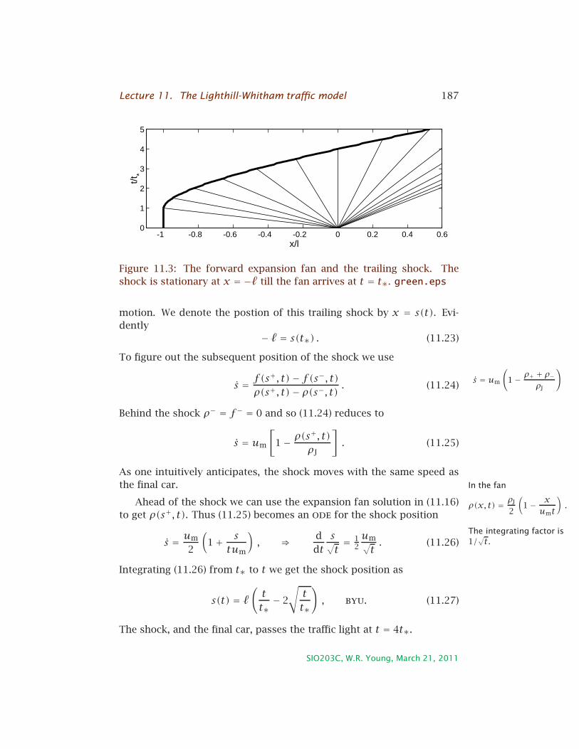
Lecture 11. The Lighthill-Whitham traffic model 187
-1 -0.8 -0.6 -0.4 -0.2 0 0.2 0.4 0.60
1
2
3
4
5
x/l
t/t*
Figure 11.3: The forward expansion fan and the trailing shock. The
shock is stationary at x = −ℓ till the fan arrives at t = t∗. green.eps
motion. We denote the postion of this trailing shock by x = s(t). Evi-
dently
− ℓ = s(t∗) . (11.23)
To figure out the subsequent position of the shock we use
s = um
(1− ρ+ + ρ−
ρJ
)
s = f(s+, t)− f(s−, t)
ρ(s+, t)− ρ(s−, t) . (11.24)
Behind the shock ρ− = f− = 0 and so (11.24) reduces to
s = um
[1− ρ(s
+, t)ρJ
]. (11.25)
As one intuitively anticipates, the shock moves with the same speed as
the final car. In the fan
ρ(x, t) = ρJ
2
(1− x
umt
).Ahead of the shock we can use the expansion fan solution in (11.16)
to get ρ(s+, t). Thus (11.25) becomes an ode for the shock position
The integrating factor is
1/√t.s = um
2
(1+ s
tum
), ⇒ d
dt
s√t= 1
2
um√t. (11.26)
Integrating (11.26) from t∗ to t we get the shock position as
s(t) = ℓ(t
t∗− 2
√t
t∗
), byu. (11.27)
The shock, and the final car, passes the traffic light at t = 4t∗.
SIO203C, W.R. Young, March 21, 2011

Lecture 11. The Lighthill-Whitham traffic model 188
-3 -2.5 -2 -1.5 -1 -0.5 0 0.5 1 1.50
0.5
1
1.5
2
ρ=ρ0
ρ=ρJ
ρ=ρ0
← x=UR
t
← x=UL t
Figure 11.4: The red light stops traffic with density ρ0 and creates two
shocks. The left going shock leaves jammed traffic behind it. red.eps
11.3 The red light problemWe use the “standard
model”:
f = umρ
(1− ρ
ρJ
)
throughout this lecture.
The shock speed is then
s = um
(1− ρ+ + ρ−
ρJ
).
Suppose we have a uniform stream of traffic with density ρ0 and sud-
denly we turn on a red light at x = 0. We assume that the first car stops
at the red light instantly and the following cars stop, building a jam with
density ρJ.
The problem is therefore
ρt + c(ρ)ρx = 0 , ρ(x,0) = ρ0 < ρJ , f (0, t) = 0 . (11.28)
There are two shocks propagating away from x = 0. The left-moving
shock has position
L(t) = −ρ0
ρJ
umt . (11.29)
This shock goes backwards into the incident traffic stream, leaving a jam
in its wake.
The right-moving shock is at
ρ− = 0 , ρ+ = ρ0
and
s = f(ρ0)
ρ0
R(t) = um
(1− ρ0
ρJ
)t . (11.30)
The last guy is congratulating himself on making it through, and the
speed of his car, u(ρ0), is also the speed on the shock.
SIO203C, W.R. Young, March 21, 2011

Lecture 11. The Lighthill-Whitham traffic model 189
11.4 Red light and green light
Now suppose we have the situation in figure 11.4 and the light turns
back to green at t = τ. What happens?
The key is to realize that there is an expansion fan solution centered
on the point (x, t) = (0, τ). This fan solution is
ρF(x, t) =ρJ
2
(1− x
(t − τ)um
), if |x| < um(t − τ) . (11.31)
The fan first interacts with the left shocks at point A in figure 11.5:
(sL, τL) =(−ρ0umτ
ρJ − ρ0,ρJτ
ρJ − ρ0
), (11.32)
And the fan reaches the right shock at point B in figure 11.5:
(sR, τR) =(u0ρJτ
ρ0,ρJτ
ρ0
). (11.33)
You can obtain these results clearly by drawing the characteristic dia-
gram and figuring out where the edges of the expansion fan at x = ±umtfirst hit the shocks in (11.29) and (11.30).
Once the fan starts to deflect the shocks the shock speed is given by
s = uFρF −u0ρ0
ρF(s, t)− ρ0= um
(1− ρ0 + ρF
ρJ
). (11.34)
Thus to determine the position of both the left and the right shock we
must integrate the ode:
s − 12
s
t − τ = um
(1
2− ρ0
ρJ
). (11.35)
The solution of (11.35) is
s(t) = um
(1− 2
ρ0
ρJ
)(t − τ)+ B
√t − τ , (11.36)
where B is the constant of integration. We can determine B using the
initial conditions in (11.32) and (11.33).
SIO203C, W.R. Young, March 21, 2011

Lecture 11. The Lighthill-Whitham traffic model 190
-1 0 1 20
0.5
1
1.5
2
2.5
3
t/τ
x/um
τ
A
B
-1 0 1 20
2
4
6
8
10
12
14
16
18
t/τ
x/um
τ
A
B
Figure 11.5: Trajectories of the shocks in the red light and green light
problem. Before the expansion fan arrives the shocks move with con-
stant speed (these are the heavy line segments). After the arrival of the
expansion fan (at points A and B) the shock paths curve. The expansion
fan produced by the Green light is centered on the point (x, t) = (0, τ).In the solution above ρ0 = 3ρJ/8 and the shock finally makes it through
the light at t = 16τ. redgreen.eps
SIO203C, W.R. Young, March 21, 2011

Lecture 11. The Lighthill-Whitham traffic model 191
For the left hand shock we find after some brutal algebra that
L(t) = um
(1− 2
ρ0
ρJ
)(t − τ)− 2um
√√√√(
1− ρ0
ρJ
)ρ0
ρJ
τ(t − τ) , if t > τL .
(11.37)
For the right hand shock we find
R(t) = um
(1− 2
ρ0
ρJ
)(t − τ)+ 2um
√√√√(
1− ρ0
ρJ
)ρ0
ρJ
τ(t − τ) , if t > τR .
(11.38)
If the traffic is light (ρ0 < ρJ/2) then the left-shock reverses direction
and eventually goes through the intersection (as shown in figure 11.5).
This happens at
τc =τ
(1− 2ρ0/ρJ)2. (11.39)
After the clearance time, τc, the congestion behind the light has dissi-
pated. An observer sitting at the light notices that at t = τc the density
drops from ρJ/2 back to ρ0. The clearance time can be distressingly long
e.g., in figure 11.5 τc = 16τ so a stopage lasting five minutes produces a
jam requiring an hour and a quarter to clear.
11.5 References
My discussion of traffic closely follows
Ha Mathematical Models: Mechanical Vibrations, Population Dynamics
and Traffic flow by Richard Haberman.
11.6 Problems
Problem 11.1. The expansion fan (11.16) is a similarity solution in which
x and t appear only in the combination η = x/umt. Substitute ρ(x, t) =R(η) into
ρt + c(ρ)ρx = 0 ,
and show that you obtain (11.13).
SIO203C, W.R. Young, March 21, 2011

Lecture 11. The Lighthill-Whitham traffic model 192
Problem 11.2. Calculate the function ρ1 in the expansion (11.15). Obtain
an explicit expression for ρ1, assuming that F is given by (11.12). Is
ǫρ1 ≪ ρ0 for all x as ǫ → 0 i.e., is the expansion uniformly valid?
Problem 11.3. Solve the expansion-fan problem
ut −u2ux = 0 , u(x,0) = H(−x) .
Sketch both the characteristic diagram and u(x,1).
Problem 11.4. Solve the expansion-fan problem
ut +uux = 0 , u(x,0) = H(x) .
Sketch both the characteristic diagram and u(x,1).
Problem 11.5. Paint flowing down a wall has a thickness η(x, t) gov-
erned by
ηt + η2ηx = 0 .
A stripe of paint is applied at t = 0 with
η(x,0) =
1 , 0 < x < 1 ,
0 , otherwise.
Find η(x, t).
Problem 11.6. For the green light solution shown in figure 11.3 draw
ρ(x, t) as a function of x at t = 0, 1/2, 1, 2, 4 and 5. Compute the
strength of the trailing shock as a function of time.
Problem 11.7. Solve the traffic problem
ρt + c(ρ)ρx = 0 , ρ(x,0) = ρJH(x) .
Draw the characteristic diagram.
Problem 11.8. Consider a more general traffic flow model with the flux
function
f(ρ) = umρ[1− (ρ/ρJ)
n] ,where n > 0 is a parameter. The special case n = 1 is the standard
model. Solve the green light problem, starting at (11.9), using this more
general model. (You can check your answer by taking n = 1 and recover-
ing the results from the lecture.) Suppose the last car (ar x = −ℓ) starts
moving at t∗ and passes through the light (x = 0) at t = t∗∗. Find the
ratio t∗∗/t∗ as a function of n and discuss the limits n→ 0 and n→∞.
SIO203C, W.R. Young, March 21, 2011

Lecture 11. The Lighthill-Whitham traffic model 193
Problem 11.9. Suppose that
f(ρ) = 120√ρ(1−√ρ) ,
where ρ is cars per mile. At t = 0 (Noon) the caravan is 2 miles long. The
airport is 15 miles away and the velocity of the lead car is
U = 120t , t measured in hours past noon.
The position of the lead car is therefore X(t) = 60t2 and so it reaches the
airport at half past noon. The plane takes off at 12:35PM. Does the last
car in the caravan arrive in time for the occupants to board the plane?
Problem 11.10. Draw ρ(x, t) as a function of x for for the solution in
figure 11.5. (Note that in this figure ρ0 = 3ρJ/8.) Choose values of t/τto illustrate how the structure of the solution changes with time.
Problem 11.11. Repeat problem 1 assuming that ρ0 = 5ρJ/8 (heavy traf-
fic). The analog of figure 11.5 is figure 11.6.
Problem 11.12. Let us develop an alternative theory for the speed of
an ρJ-plug behind a red light. Suppose the cars are all initially moving
at u(ρ0) and consider car n + 1 behind the light. The initial distance
between this car and the light is then n/ρ0. (i) How far will this car be
from the light when it is forced to stop? Call this stopping distance Xn.
(ii) Assuming instant decceleration from u0 to rest, how long it take car
n + 1 to stop? Call this stopping time Tn. (iii) Eliminate n between Xnand Tn and show that the line of stopped vehicles moves backwards with
the speed UL in (11.29).
Problem 11.13. Give a simpler derivation of the clearence time in (11.39).
First show that
Number of cars through the light between τ and τc = fm(τc − τ) .
Also show that
Number of cars slowed by the light = f(ρ0)τc .
Equating these two numbers show that
τc =fm
fm − f0. (11.40)
Show that for the standard model (11.40) reduces to (11.39).
SIO203C, W.R. Young, March 21, 2011

Lecture 11. The Lighthill-Whitham traffic model 194
-2 -1 0 10
0.5
1
1.5
2
2.5
3
t/τ
x/um
τ
A
B
-2 -1 0 10
2
4
6
8
10
12
14
16
18
t/τ
x/um
τ
A
B
Figure 11.6: Shock trajectories if ρ0 = 5ρJ/8 (heavy traffic). rgprob.eps
SIO203C, W.R. Young, March 21, 2011