Sinusoidal waveform. Instantaneous and RMS values. … notes/Lectures notes...Circuits with...
24
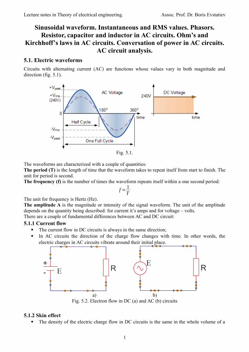
Lecture notes in Theory of electrical engineering. Assoc. Prof. Dr. Boris Evstatiev Sinusoidal waveform. Instantaneous and RMS values. Phasors. Resistor, capacitor and inductor in AC circuits. Ohm’s and Kirchhoff’s laws in AC circuits. Conversation of power in AC circuits. AC circuit analysis. 5.1. Electric waveforms Circuits with alternating current (AC) are functions whose values vary in both magnitude and direction (fig. 5.1). Fig. 5.1. The waveforms are characterized with a couple of quantities: The period (T) is the length of time that the waveform takes to repeat itself from start to finish. The unit for period is second. The frequency (f) is the number of times the waveform repeats itself within a one second period: f = 1 T The unit for frequency is Hertz (Hz). The amplitude A is the magnitude or intensity of the signal waveform. The unit of the amplitude depends on the quantity being described: for current it’s amps and for voltage – volts. There are a couple of fundamental differences between AC and DC circuit: 5.1.1 Current flow The current flow in DC circuits is always in the same direction; In AC circuits the direction of the charge flow changes with time. In other words, the electric charges in AC circuits vibrate around their initial place. a) b) Fig. 5.2. Electron flow in DC (a) and AC (b) circuits 5.1.2 Skin effect The density of the electric charge flow in DC circuits is the same in the whole volume of a 1
Transcript of Sinusoidal waveform. Instantaneous and RMS values. … notes/Lectures notes...Circuits with...
Lecture notes in Theory of electrical engineering. Assoc. Prof. Dr. Boris Evstatiev
Sinusoidal waveform. Instantaneous and RMS values. Phasors.Resistor, capacitor and inductor in AC circuits. Ohm’s and
Kirchhoff’s laws in AC circuits. Conversation of power in AC circuits.AC circuit analysis.
5.1. Electric waveforms
Circuits with alternating current (AC) are functions whose values vary in both magnitude anddirection (fig. 5.1).
Fig. 5.1.
The waveforms are characterized with a couple of quantities: The period (T) is the length of time that the waveform takes to repeat itself from start to finish. Theunit for period is second.The frequency (f) is the number of times the waveform repeats itself within a one second period:
f =1T
The unit for frequency is Hertz (Hz).The amplitude A is the magnitude or intensity of the signal waveform. The unit of the amplitudedepends on the quantity being described: for current it’s amps and for voltage – volts.There are a couple of fundamental differences between AC and DC circuit:
5.1.1 Current flow The current flow in DC circuits is always in the same direction; In AC circuits the direction of the charge flow changes with time. In other words, the
electric charges in AC circuits vibrate around their initial place.
a) b)Fig. 5.2. Electron flow in DC (a) and AC (b) circuits
5.1.2 Skin effect The density of the electric charge flow in DC circuits is the same in the whole volume of a
1
Lecture notes in Theory of electrical engineering. Assoc. Prof. Dr. Boris Evstatiev
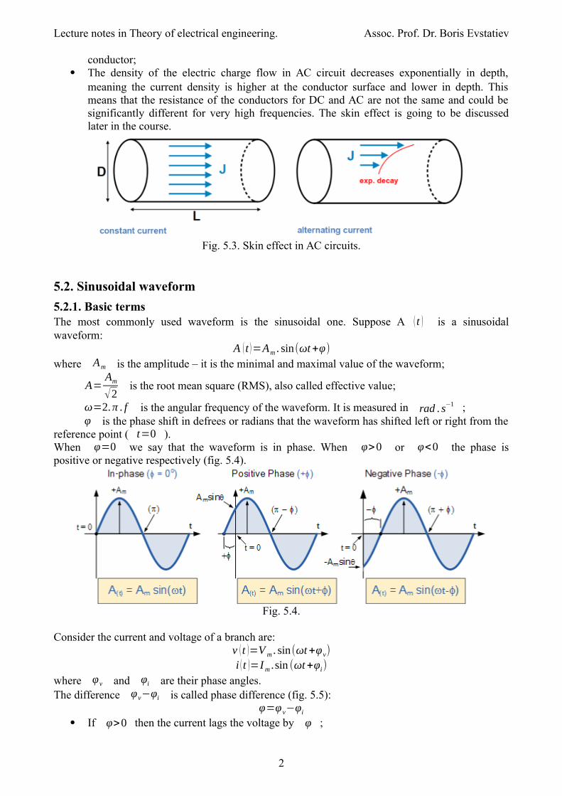
conductor; The density of the electric charge flow in AC circuit decreases exponentially in depth,
meaning the current density is higher at the conductor surface and lower in depth. Thismeans that the resistance of the conductors for DC and AC are not the same and could besignificantly different for very high frequencies. The skin effect is going to be discussedlater in the course.
Fig. 5.3. Skin effect in AC circuits.
5.2. Sinusoidal waveform
5.2.1. Basic termsThe most commonly used waveform is the sinusoidal one. Suppose A ( t ) is a sinusoidalwaveform:
A (t )=Аm . sin(ωt+φ)
where Am is the amplitude – it is the minimal and maximal value of the waveform;
A=Am
√2 is the root mean square (RMS), also called effective value;
ω=2.π . f is the angular frequency of the waveform. It is measured in rad . s−1 ;φ is the phase shift in defrees or radians that the waveform has shifted left or right from the
reference point ( t=0 ).When φ=0 we say that the waveform is in phase. When φ>0 or φ<0 the phase ispositive or negative respectively (fig. 5.4).
Fig. 5.4.
Consider the current and voltage of a branch are:v (t )=V m . sin(ωt+φv)
i (t )=Im .sin (ωt+φi)
where φv and φi are their phase angles.The difference φv−φi is called phase difference (fig. 5.5):
φ=φ v−φi
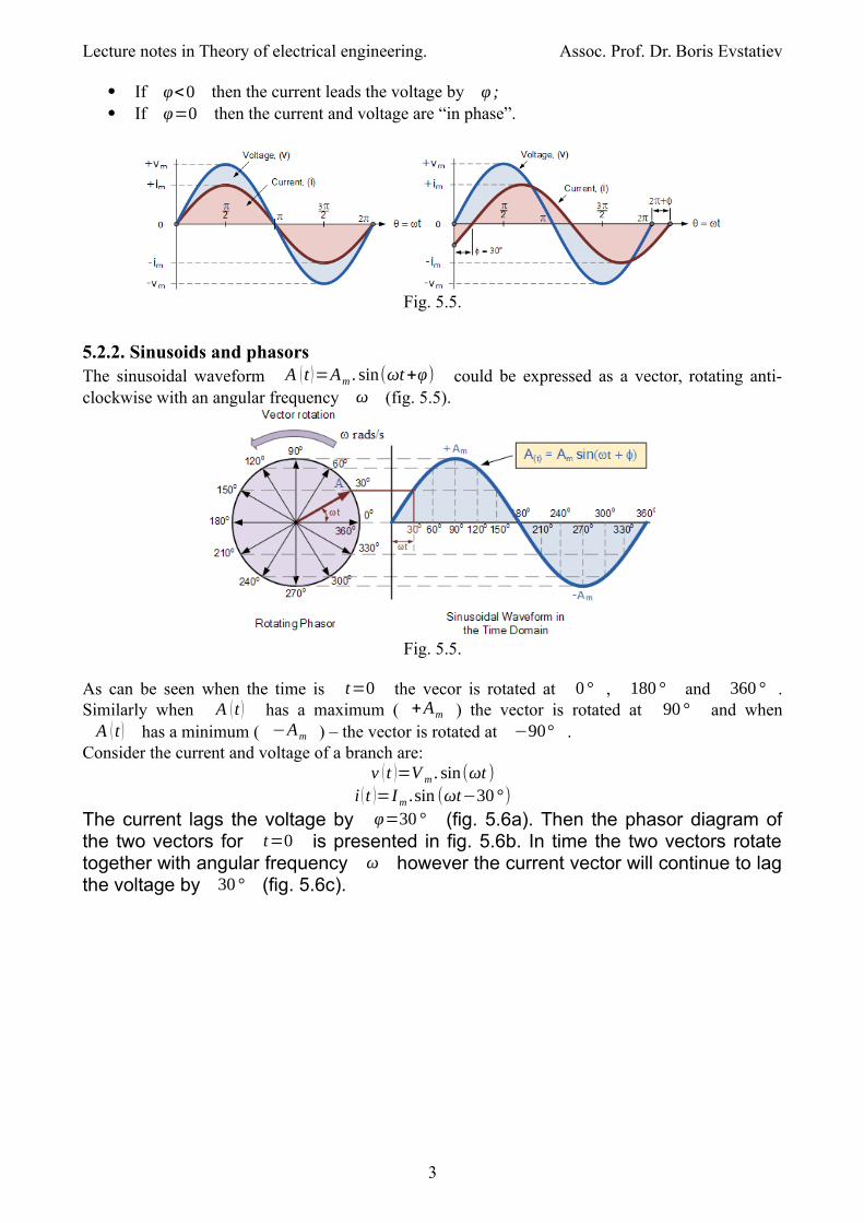
If φ>0 then the current lags the voltage by φ ;
2
Lecture notes in Theory of electrical engineering. Assoc. Prof. Dr. Boris Evstatiev
If φ<0 then the current leads the voltage by φ; If φ=0 then the current and voltage are “in phase”.
Fig. 5.5.
5.2.2. Sinusoids and phasorsThe sinusoidal waveform А (t )=Аm . sin(ωt+φ) could be expressed as a vector, rotating anti-clockwise with an angular frequency ω (fig. 5.5).
Fig. 5.5.
As can be seen when the time is t=0 the vecor is rotated at 0 ° , 180 ° and 360 ° .Similarly when A (t ) has a maximum ( +Am ) the vector is rotated at 90 ° and when
A ( t ) has a minimum ( −Am ) – the vector is rotated at −90° .Consider the current and voltage of a branch are:
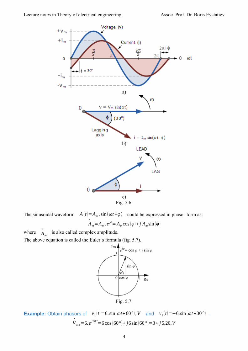
v (t )=V m . sin(ωt )i (t )=Im .sin (ωt−30 °)
The current lags the voltage by φ=30 ° (fig. 5.6a). Then the phasor diagram ofthe two vectors for t=0 is presented in fig. 5.6b. In time the two vectors rotatetogether with angular frequency ω however the current vector will continue to lagthe voltage by 30 ° (fig. 5.6c).
3
Lecture notes in Theory of electrical engineering. Assoc. Prof. Dr. Boris Evstatiev
a)
b)
c)Fig. 5.6.
The sinusoidal waveform А (t )=Аm . sin(ωt+φ) could be expressed in phasor form as:
А•
m=Am . e jφ=Amcos (φ )+ j Am sin (φ )
where А•
m is also called complex amplitude.
The above equation is called the Euler‘s formula (fig. 5.7).
Fig. 5.7.
Example: Obtain phasors of v1 ( t )=6. sin (ωt+60° ) ,V and v2 (t )=−6.sin (ωt+30 ° ) .
V•
m1=6.e j60 °=6cos (60° )+ j6sin (60 ° )=3+ j 5.20,V
4
Lecture notes in Theory of electrical engineering. Assoc. Prof. Dr. Boris Evstatiev
V•
m2=−6.e j30°=−6cos (30 ° )− j6sin (30 ° )=−5.20− j3We can also use the RMS phasors:
V•
1=6√2
e j60 °=4.24cos (60 ° )+ j 4.24 sin (60 ° )=2.12+ j3.67,V
V•
2=−6√2
. e j30 °=−4.24 cos (30° )− j 4.24sin (30 ° )=−3.67− j 2.12,V
Example: Obtain the sinusoids of the peak phasors V•
m1=2+ j5 and the RMS phasor
V•
2=5− j 1 .
First we convert the phasors in polar form:
V•
m1=2+ j5=√22+52 . ej atan 5
2=5.34 e j68.2°
V•
2=5− j 1=√52+12 . e
j atan −15 =5.1 e− j11.3°
Then we can write down the sine values:v1 (t )=5.34 sin (ωt+68.2° ) ,V
v2 ( t )=5.1.√2sin (ωt−11.3° )=7.21 . sin (ωt−11.3° ) ,V
5.3. Sinusoidal steady state
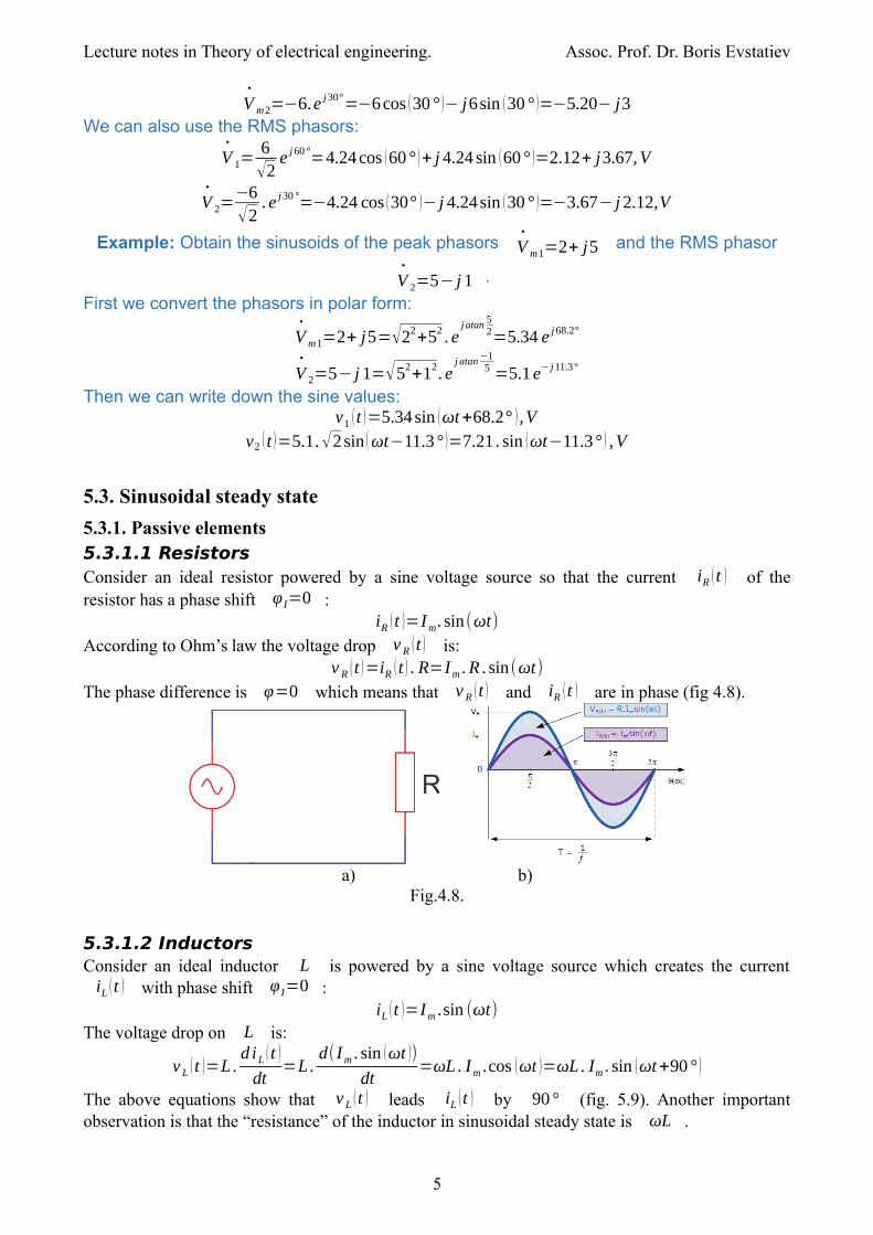
5.3.1. Passive elements5.3.1.1 ResistorsConsider an ideal resistor powered by a sine voltage source so that the current iR (t ) of theresistor has a phase shift φ I=0 :
iR (t )=Im. sin(ωt)
According to Ohm’s law the voltage drop v R (t ) is:v R (t )=iR (t ) . R=Im . R .sin(ωt)
The phase difference is φ=0 which means that v R (t ) and iR (t ) are in phase (fig 4.8).
a) b)Fig.4.8.
5.3.1.2 InductorsConsider an ideal inductor L is powered by a sine voltage source which creates the currentiL (t ) with phase shift φ I=0 :
iL (t )=Im .sin (ωt)The voltage drop on L is:
v L (t )=L .d iL ( t )
dt=L .
d(Im . sin (ωt ))
dt=ωL. Im .cos (ωt )=ωL. Im . sin (ωt+90 ° )
The above equations show that v L (t ) leads iL ( t ) by 90 ° (fig. 5.9). Another importantobservation is that the “resistance” of the inductor in sinusoidal steady state is ωL .
5
Lecture notes in Theory of electrical engineering. Assoc. Prof. Dr. Boris Evstatiev
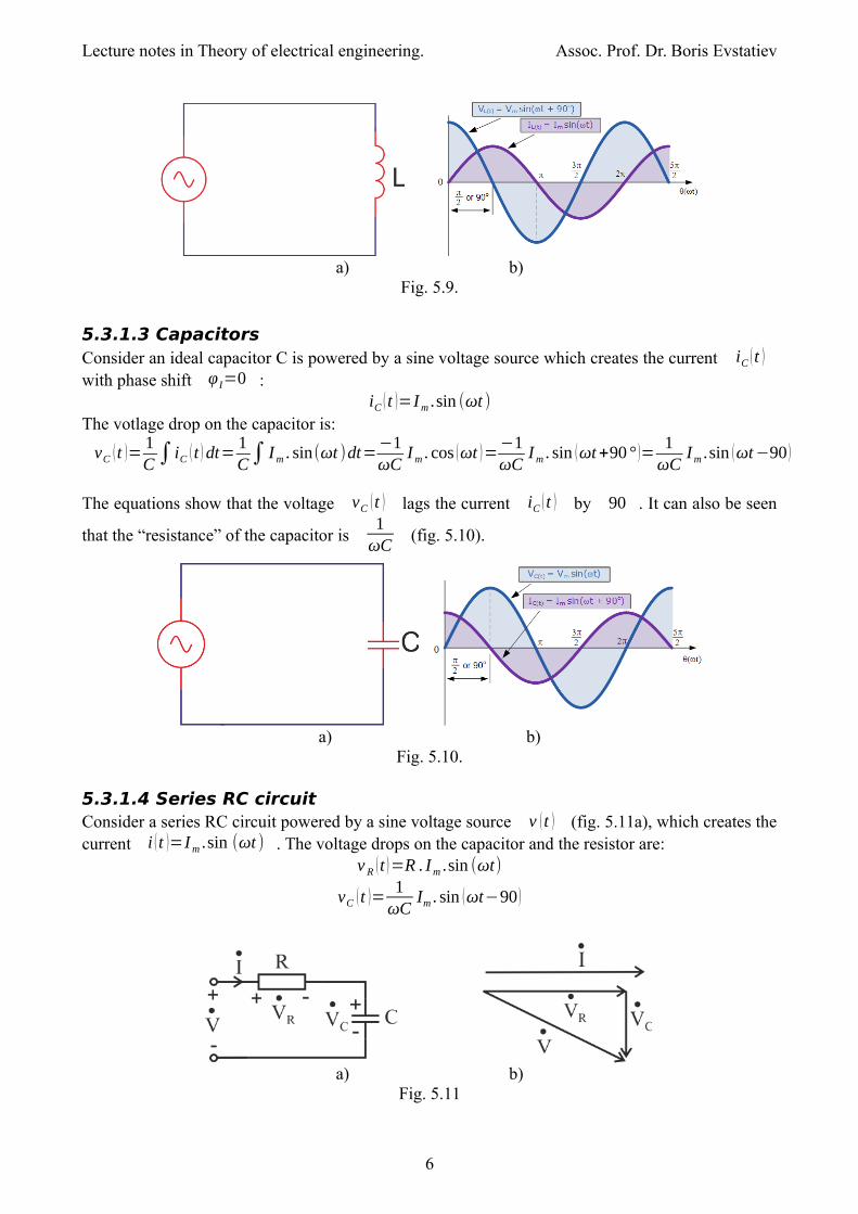
a) b)Fig. 5.9.
5.3.1.3 CapacitorsConsider an ideal capacitor C is powered by a sine voltage source which creates the current iC (t )
with phase shift φ I=0 :iC ( t )=Im .sin (ωt )
The votlage drop on the capacitor is:
vC (t )=1C∫ iC (t ) dt=
1C∫ Im . sin(ωt )dt=
−1ωC
Im .cos (ωt )=−1ωC
Im . sin (ωt+90 ° )=1
ωCIm .sin (ωt−90 )
The equations show that the voltage vC (t ) lags the current iC ( t ) by 90 . It can also be seen
that the “resistance” of the capacitor is 1
ωC (fig. 5.10).
a) b)Fig. 5.10.
5.3.1.4 Series RC circuitConsider a series RC circuit powered by a sine voltage source v ( t ) (fig. 5.11a), which creates thecurrent i (t )=Im .sin (ωt ) . The voltage drops on the capacitor and the resistor are:
v R (t )=R . Im .sin (ωt)
vC (t )=1
ωCIm . sin (ωt−90 )
a) b)Fig. 5.11
6

Lecture notes in Theory of electrical engineering. Assoc. Prof. Dr. Boris Evstatiev
The above equations could be written with phasors as:
I•
=Im
√2e j0
=I
V•
R=R I e j0=R I•
V•
C=1
ωCIme− j90°
=XC e− j90 ° I•
The vector diagram of of the voltages and current are presented in fig. 5.11b. It could be seen thatthe source voltage is:
V•
=V•
R+V•
C=I•
(R+XCe− j90 ° )=I
•
(R− j XC )
In other words the complex impedance of the capacitor is − j XC or − j1
ωC where
1ωC
is
the capacitive reactance of the capacitor in Ohms.5.3.1.5 Series RL circuitConsider a series RL circuit powered by a sinusoidal voltage source v ( t ) (fig. 5.12a), whichcreates the current i (t )=Im .sin (ωt ) . The phasor values are:
I•
=Im
√2e j0
=I
V•
R=R I e j0=R I•
V•
L=ωL I e j90°=X Le
j90 ° I•
a) b)Fig. 5.12
The vector diagram is presented in fig. 5.12b and the source voltage is:
V•
=V•
R+V•
L=I•
(R+X Lej90 ° )=I
•
(R+ j XL )The quantity j X L= jωL is the complex impedance of the inductor where ωL is the inductivereactance in Ohms.5.3.1.6 Series RLC circuitConsider a series RLC circuit powered by a sine voltage source v (t ) , which creats a currenti (t )=Im .sin (ωt ) (4.13). As was already demonstrated the phasor voltage drops on the three
passive elements are:
I•
=Im
√2e j0
=I
V•
R=I•
R
V•
L=I•
ωLe j90°=I•
XLej 90°
V•
C=I• 1ωC
e− j 90°=I
•
XC e− j90 °
7
Lecture notes in Theory of electrical engineering. Assoc. Prof. Dr. Boris Evstatiev
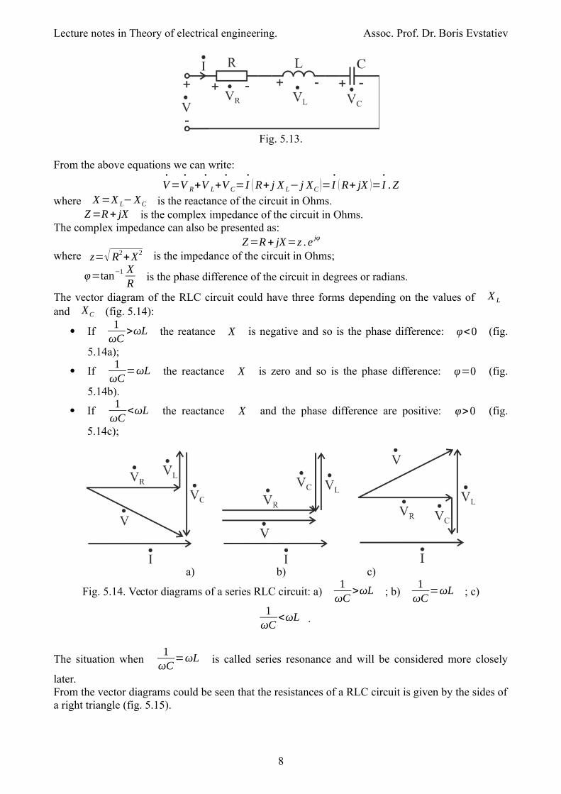
Fig. 5.13.
From the above equations we can write:
V•
=V•
R+V•
L+V•
C=I•
(R+ j X L− j XC )=I•
( R+ jX )=I•
. Z
where X=X L−XC is the reactance of the circuit in Ohms.Z=R+ jX is the complex impedance of the circuit in Ohms.
The complex impedance can also be presented as:Z=R+ jX=z . e jφ
where z=√R2+X2 is the impedance of the circuit in Ohms;
φ=tan−1 XR
is the phase difference of the circuit in degrees or radians.
The vector diagram of the RLC circuit could have three forms depending on the values of X L
and XC (fig. 5.14):
If 1
ωC>ωL the reatance X is negative and so is the phase difference: φ<0 (fig.
5.14a);
If 1
ωC=ωL the reactance X is zero and so is the phase difference: φ=0 (fig.
5.14b).
If 1
ωC<ωL the reactance X and the phase difference are positive: φ>0 (fig.
5.14c);
a) b) c)
Fig. 5.14. Vector diagrams of a series RLC circuit: a) 1
ωC>ωL ; b)
1ωC
=ωL ; c)
1ωC
<ωL .
The situation when 1
ωC=ωL is called series resonance and will be considered more closely
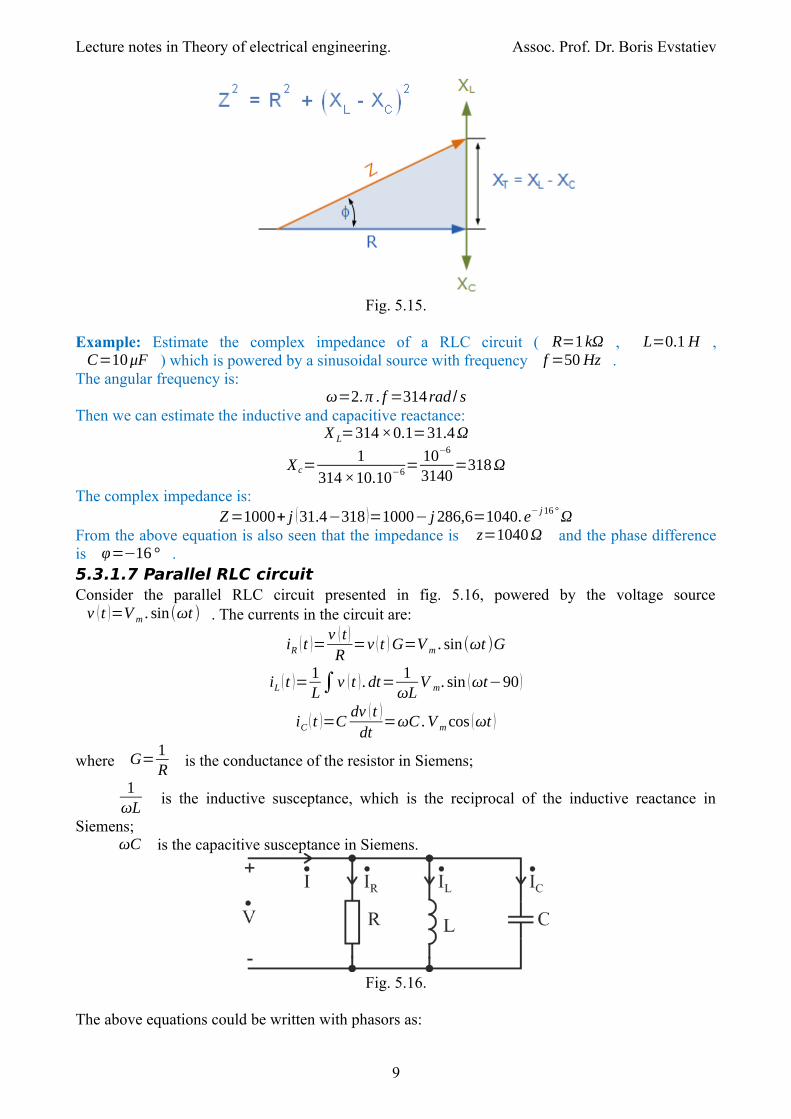
later.From the vector diagrams could be seen that the resistances of a RLC circuit is given by the sides ofa right triangle (fig. 5.15).
8
Lecture notes in Theory of electrical engineering. Assoc. Prof. Dr. Boris Evstatiev
Fig. 5.15.
Example: Estimate the complex impedance of a RLC circuit ( R=1kΩ , L=0.1 H ,C=10μF ) which is powered by a sinusoidal source with frequency f =50 Hz .
The angular frequency is:ω=2.π . f =314 rad / s
Then we can estimate the inductive and capacitive reactance:X L=314×0.1=31.4Ω
X c=1
314×10.10−6=10−6
3140=318Ω
The complex impedance is:Z=1000+ j (31.4−318 )=1000− j 286,6=1040. e− j16 °Ω
From the above equation is also seen that the impedance is z=1040Ω and the phase differenceis φ=−16 ° .5.3.1.7 Parallel RLC circuitConsider the parallel RLC circuit presented in fig. 5.16, powered by the voltage sourcev (t )=V m . sin(ωt ) . The currents in the circuit are:
iR (t )=v (t )
R=v (t ) G=V m . sin(ωt )G
iL (t )=1L∫v (t ) . dt=
1ωL
V m. sin (ωt−90 )
iC (t )=Cdv (t )
dt=ωC.V m cos (ωt )
where G=1R
is the conductance of the resistor in Siemens;
1ωL
is the inductive susceptance, which is the reciprocal of the inductive reactance in
Siemens;ωC is the capacitive susceptance in Siemens.
Fig. 5.16.
The above equations could be written with phasors as:
9
Lecture notes in Theory of electrical engineering. Assoc. Prof. Dr. Boris Evstatiev
V•
=V m
√2e j0
=V
I•
R=V•
G
I•
L=V• 1ωL
e− j90 °=V
•
BL e− j90°
I•
C=V•
ωCe j90 °=V•
BC e j90 °
Then the total current coming from the source is:
I•
=I•
R+ I•
L+ I•
C=V•
(G− j (BL−BC ))=V•
(G− jB )=V•
.Y
where B=BL−BC is the susceptance of the circuit in Siemens.Y=G− jB is the complex admitance of the circuit in Siemens.
The complex admitance can also be presented as:Y=G− jB= y . e− jφ
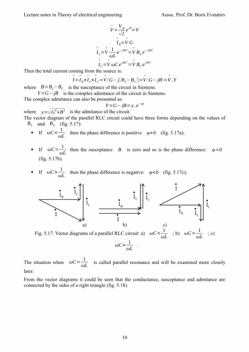
where y=√G2+B2 is the admitance of the circuit.The vector diagram of the parallel RLC circuit could have three forms depending on the values ofBL and BC (fig. 5.17):
If ωC<1ωL
then the phase difference is positive φ>0 (fig. 5.17a);
If ωC=1ωL
then the susceptance B is zero and so is the phase difference: φ=0
(fig. 5.17b).
If ωC>1ωL
then the phase difference is negative: φ<0 (fig. 5.17c);
a) b) c)
Fig. 5.17. Vector diagrams of a parallel RLC circuit: a) ωC<1ωL
; b) ωC=1ωL
; c)
ωC>1ωL
.
The situation when ωC=1ωL
is called parallel resonance and will be examined more closely
later.
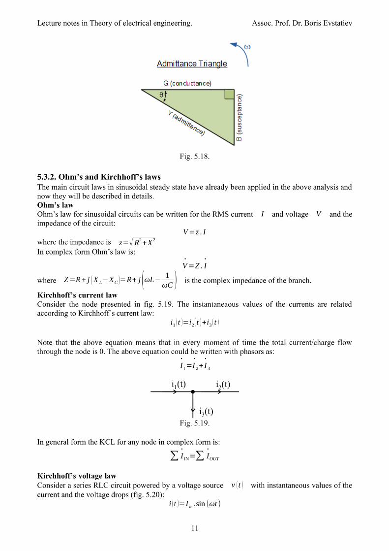
From the vector diagrams it could be seen that the conductance, susceptance and admitance areconnected by the sides of a right triangle (fig. 5.18).
10
Lecture notes in Theory of electrical engineering. Assoc. Prof. Dr. Boris Evstatiev
Fig. 5.18.
5.3.2. Ohm’s and Kirchhoff’s lawsThe main circuit laws in sinusoidal steady state have already been applied in the above analysis andnow they will be described in details.Ohm’s lawOhm’s law for sinusoidal circuits can be written for the RMS current I and voltage V and theimpedance of the circuit:
V=z . Iwhere the impedance is z=√R2+X2
In complex form Ohm’s law is:
V•
=Z . I•
where Z=R+ j (X L−XC )=R+ j(ωL−1
ωC ) is the complex impedance of the branch.
Kirchhoff’s current lawConsider the node presented in fig. 5.19. The instantaneaous values of the currents are relatedaccording to Kirchhoff’s current law:
i1 (t )=i2 (t )+i3 (t )
Note that the above equation means that in every moment of time the total current/charge flowthrough the node is 0. The above equation could be written with phasors as:
I•
1=I•
2+ I•
3
Fig. 5.19.
In general form the KCL for any node in complex form is:
∑ I•
IN=∑ I•
OUT
Kirchhoff’s voltage lawConsider a series RLC circuit powered by a voltage source v (t ) with instantaneous values of thecurrent and the voltage drops (fig. 5.20):
i (t )=Im .sin (ωt )
11
Lecture notes in Theory of electrical engineering. Assoc. Prof. Dr. Boris Evstatiev
v R (t )=R . Im .sin (ωt)
v L (t )=L .di (t )
dt=ωL. Im. sin (ωt+90 ° )=ωL. Imcos (ωt )
vC (t )=1C
.∫ i (t ) . dt+uC (0 )=1
ωCIm . sin (ωt−90 )=
−1ωC
Imcos (ωt )
Fig. 5.20.
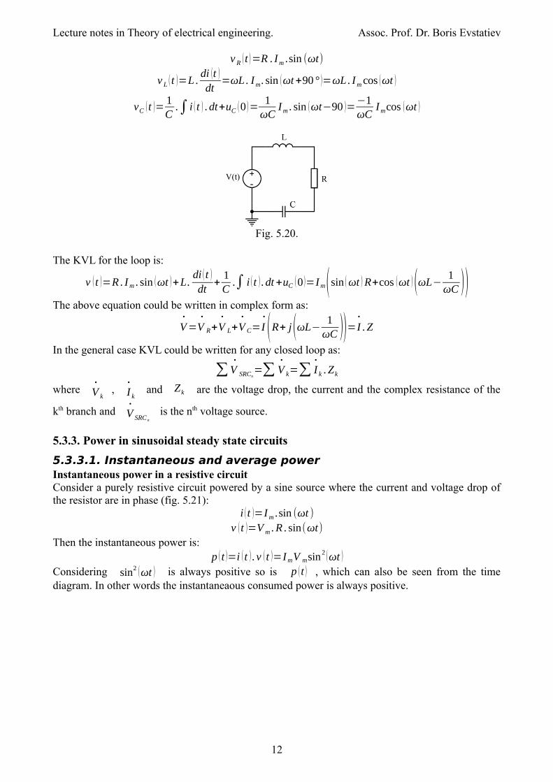
The KVL for the loop is:
v (t )=R . Im . sin (ωt )+L.di (t )
dt+
1C
.∫ i (t ) . dt+uC (0 )=Im(sin ( ωt ) R+cos (ωt )(ωL−1
ωC ))The above equation could be written in complex form as:
V•
=V•
R+V•
L+V•
C=I•
(R+ j(ωL−1
ωC ))=I•
. Z
In the general case KVL could be written for any closed loop as:
∑V•
SRCn=∑ V
•
k=∑ I•
k . Zk
where V•
k, I
•
k and Zk are the voltage drop, the current and the complex resistance of the
kth branch and V•
SRC n
is the nth voltage source.
5.3.3. Power in sinusoidal steady state circuits
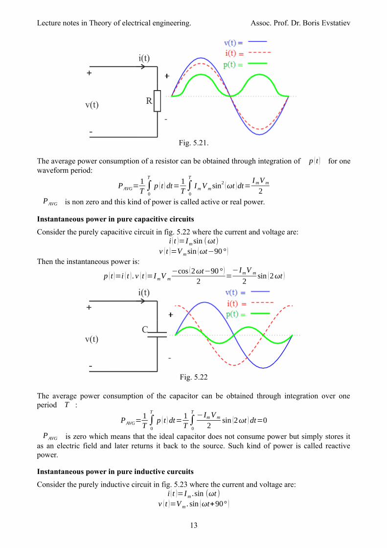
5.3.3.1. Instantaneous and average powerInstantaneous power in a resistive circuitConsider a purely resistive circuit powered by a sine source where the current and voltage drop ofthe resistor are in phase (fig. 5.21):
i (t )=Im .sin (ωt )v (t )=V m .R . sin(ωt)
Then the instantaneous power is:p (t )=i (t ) . v (t )=ImV msin
2 (ωt )
Considering sin2 (ωt ) is always positive so is p (t ) , which can also be seen from the timediagram. In other words the instantaneaous consumed power is always positive.
12
Lecture notes in Theory of electrical engineering. Assoc. Prof. Dr. Boris Evstatiev
Fig. 5.21.
The average power consumption of a resistor can be obtained through integration of p (t ) for onewaveform period:
PAVG=1T∫0
T
p ( t ) dt=1T∫0
T
ImV m sin2 (ωt )dt=ImV m
2PAVG is non zero and this kind of power is called active or real power.
Instantaneous power in pure capacitive circuits
Consider the purely capacitive circuit in fig. 5.22 where the current and voltage are:i (t )=Im sin (ωt)
v (t )=V m sin (ωt−90 ° )
Then the instantaneous power is:
p (t )=i ( t ) . v (t )=ImV m
−cos (2ωt−90 ° )
2=
−ImV m
2sin (2ωt )
Fig. 5.22
The average power consumption of the capacitor can be obtained through integration over oneperiod T :
PAVG=1T∫0
T
p ( t ) dt=1T∫0
T−ImV m
2sin (2ωt ) dt=0
PAVG is zero which means that the ideal capacitor does not consume power but simply stores itas an electric field and later returns it back to the source. Such kind of power is called reactivepower.
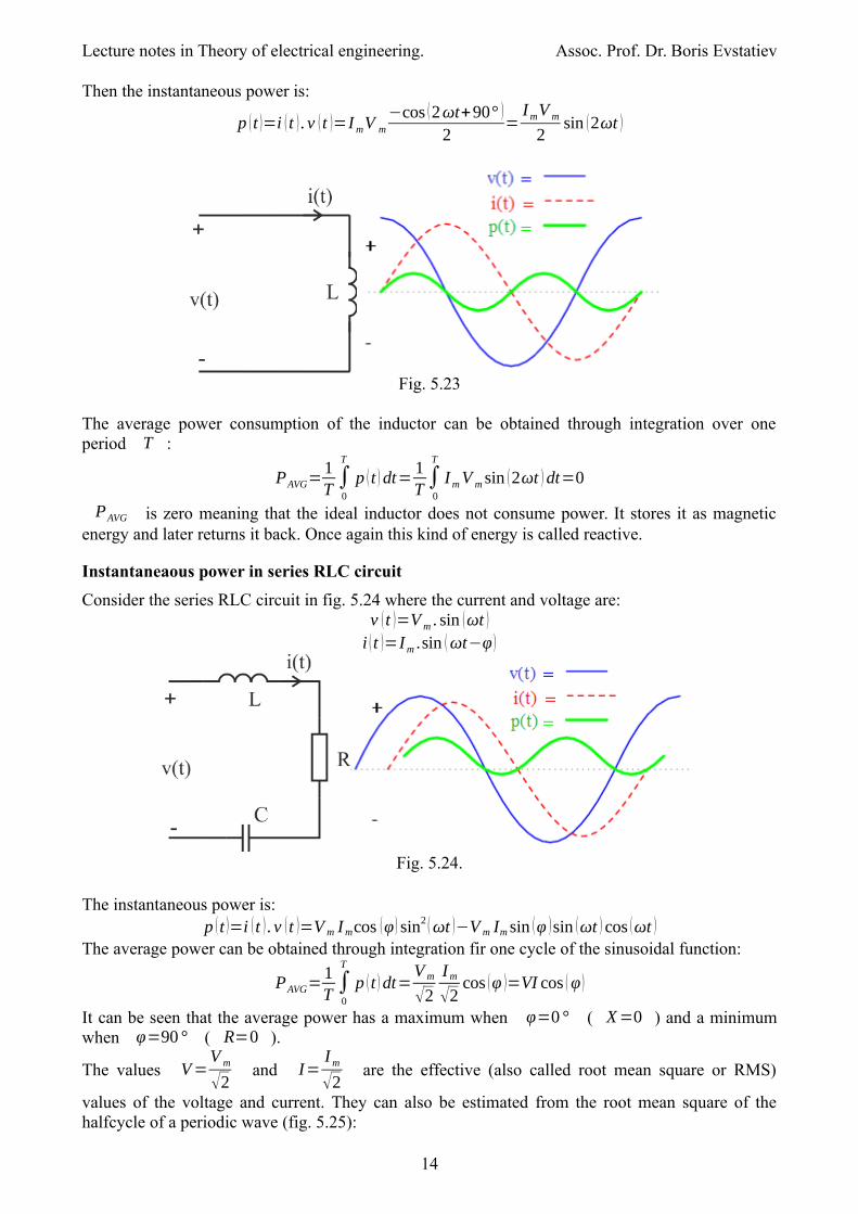
Instantaneous power in pure inductive curcuits
Consider the purely inductive circuit in fig. 5.23 where the current and voltage are:i (t )=Im .sin (ωt )
v (t )=V m . sin (ωt+90° )
13
Lecture notes in Theory of electrical engineering. Assoc. Prof. Dr. Boris Evstatiev
Then the instantaneous power is:
p (t )=i ( t ) . v (t )=ImV m
−cos (2ωt+90° )
2=
ImV m
2sin (2ωt )
Fig. 5.23
The average power consumption of the inductor can be obtained through integration over oneperiod T :
PAVG=1T∫0
T
p ( t ) dt=1T∫0
T
ImV m sin (2ωt ) dt=0
PAVG is zero meaning that the ideal inductor does not consume power. It stores it as magneticenergy and later returns it back. Once again this kind of energy is called reactive.
Instantaneaous power in series RLC circuit
Consider the series RLC circuit in fig. 5.24 where the current and voltage are:v (t )=V m . sin (ωt )
i (t )=Im .sin (ωt−φ )
Fig. 5.24.
The instantaneous power is:p (t )=i (t ) . v (t )=V m Imcos (φ ) sin2 (ωt )−V m Im sin (φ )sin (ωt ) cos (ωt )
The average power can be obtained through integration fir one cycle of the sinusoidal function:
PAVG=1T∫0
T
p (t ) dt=V m
√2
Im
√2cos (φ )=VI cos ( φ )
It can be seen that the average power has a maximum when φ=0 ° ( X=0 ) and a minimumwhen φ=90 ° ( R=0 ).
The values V=V m
√2 and I=
Im
√2 are the effective (also called root mean square or RMS)
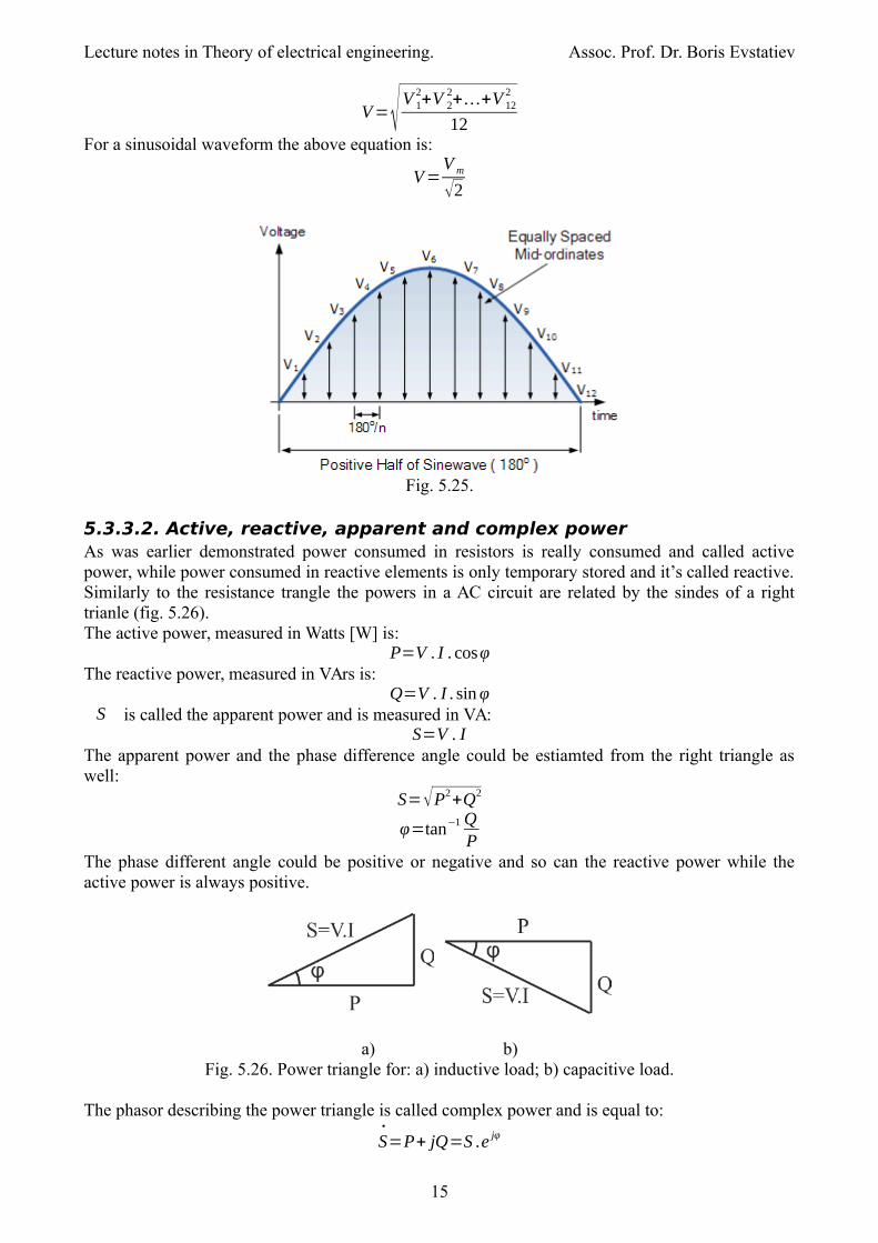
values of the voltage and current. They can also be estimated from the root mean square of thehalfcycle of a periodic wave (fig. 5.25):
14
Lecture notes in Theory of electrical engineering. Assoc. Prof. Dr. Boris Evstatiev
V=√V 12+V 2
2+…+V 12
2
12For a sinusoidal waveform the above equation is:
V=V m
√2
Fig. 5.25.
5.3.3.2. Active, reactive, apparent and complex powerAs was earlier demonstrated power consumed in resistors is really consumed and called activepower, while power consumed in reactive elements is only temporary stored and it’s called reactive.Similarly to the resistance trangle the powers in a AC circuit are related by the sindes of a righttrianle (fig. 5.26).The active power, measured in Watts [W] is:
P=V . I .cosφThe reactive power, measured in VArs is:
Q=V . I . sinφS is called the apparent power and is measured in VA:
S=V . IThe apparent power and the phase difference angle could be estiamted from the right triangle aswell:
S=√P2+Q2
φ=tan−1 QP
The phase different angle could be positive or negative and so can the reactive power while theactive power is always positive.
a) b)Fig. 5.26. Power triangle for: a) inductive load; b) capacitive load.
The phasor describing the power triangle is called complex power and is equal to:
S•
=P+ jQ=S .e jφ
15
Lecture notes in Theory of electrical engineering. Assoc. Prof. Dr. Boris Evstatiev
Similarly to the apparent power the complex power is measured in VA.
5.3.3.3. Conservatino of power in AC circuits
Following the conservation of energy law power should be conserved in AC circuits. Thisconservation is defined as:
∑ S•
SRC=∑ S•
CONS
where S•
SRC and S
•
CONS are the cumulative complex powers of the sources and consumers
respectively. Since S•
=P+ jQ , the above equation could also be written individually for the
active and reactive power in the circuit:∑ PSRC=∑ PCONS
and ∑QSRC=∑ QCONS
Power of the consumersThe active and reactive power for a certain branch of the circuit can be estimated respectively with:
P=I 2. RQ=I 2.(ωL−1
ωC )Power of the sources
Consider the current flow through a voltage source V•
V is I
•
V. Then the complex power of the
voltage source is:
S•
V=V•
V . I*
I
where I*
I is the complex conjugate of the current:
I•
V=IV . e jφ→I*
I=IV . e− jφ
Next consider the current source I•
I with a voltage drop U
•
I. The complex power of the
votlage is:
S•
I=V•
I . I*
I
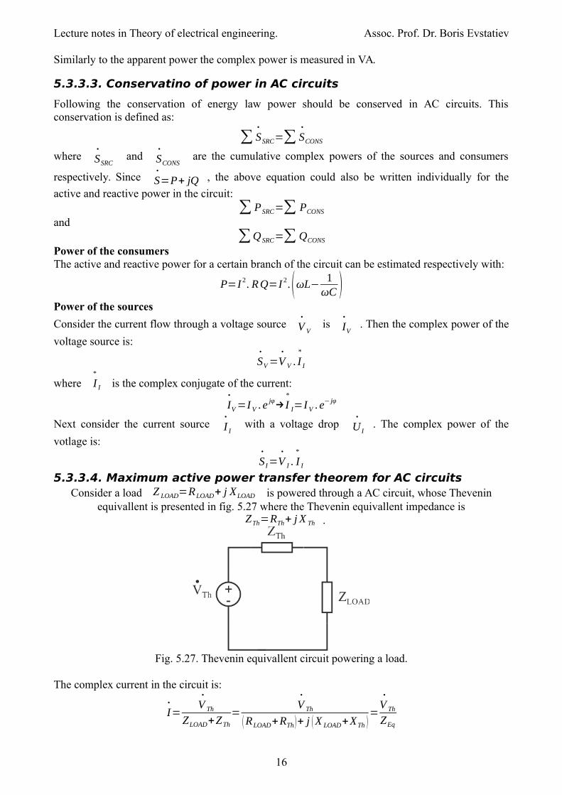
5.3.3.4. Maximum active power transfer theorem for AC circuitsConsider a load Z LOAD=RLOAD+ j XLOAD is powered through a AC circuit, whose Thevenin
equivallent is presented in fig. 5.27 where the Thevenin equivallent impedance isZTh=RTh+ j X Th .
Fig. 5.27. Thevenin equivallent circuit powering a load.
The complex current in the circuit is:
I•
=V•
Th
ZLOAD+ZTh
=V•
Th
(RLOAD+RTh)+ j (X LOAD+XTh )=
V•
Th
ZEq
16
Lecture notes in Theory of electrical engineering. Assoc. Prof. Dr. Boris Evstatiev
The equivallent resistance Z Eq can be presented in polar form as:
Z Eq=√ (RLOAD+RTh )2+( XLOAD+XTh )
2ej atan
X LOAD+XTh
RLOAD+R Th =z . e jφ
where the phase difference is φ=atanX LOAD+XTh
RLOAD+RTh and the impedance of the circuit is
z=√ (RLOAD+RTh )2+( XLOAD+XTh)
2 .The active power reaching the load is:
P=V Th . I .cosφ=V Th
2
√(RLOAD+RTh )2+(X LOAD+XTh )
2cos φ
As can be seen from the above equation the two requirements to have maximal power are: cosφ should have a maximum. This happens when:
cosφ=1→atanX LOAD+XTh
RLOAD+RTh
=0→X LOAD=−XTh
The denominator should have a minimum:
√ (RLOAD+RTh )2+( XLOAD+XTh )
2=MIN
If the reactive part of the denominator is removed ( X LOAD=−X Th the denominator becomeslowest. Considering this is also a requirement for the maximum of cosφ=1 we apply it andobtain a purely resistive denominator:
√ (RLOAD+RTh )2+( XLOAD+XTh)
2=√(RLOAD+RTh )
2=RLOAD+RTh
We have already proven for DC circuit that for resistive circuits the power transfer is maximal ifRLOAD=RTh . Then the active power reaching the load is maximal when the complex load
impedance equals the complex conjugate of the Thevenin’s complex impedance:
Z•
LOAD=Z*
Th
5.4. Analysis of circuits in sinusoidal steady state
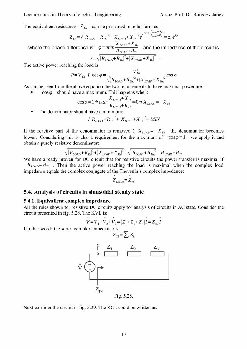
5.4.1. Equivallent complex impedanceAll the rules shown for resistive DC circuits apply for analysis of circuits in AC state. Consider thecircuit presented in fig. 5.28. The KVL is:
V•
=V•
1+V•
2+V•
3= (Z1+Z2+Z3 ) I•
=Z IN I•
In other words the series complex impedance is:Z IN=∑ Zk
Fig. 5.28.
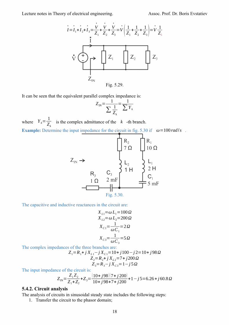
Next consider the circuit in fig. 5.29. The KCL could be written as:
17
Lecture notes in Theory of electrical engineering. Assoc. Prof. Dr. Boris Evstatiev
I•
=I•
1+ I•
2+ I•
3=V•
Z1
+V•
Z2
+V•
Z3
=V•
( 1Z1
+1Z2
+1Z3
)=V• 1Z¿
Fig. 5.29.
It can be seen that the equivalent parallel complex impedance is:
Z IN=1
∑1Zk
=1
∑Y k
where Y k=1Zk
is the complex admittance of the k -th branch.
Example: Determine the input impedance for the circuit in fig. 5.30 if ω=100 rad /s .
Fig. 5.30.
The capacitive and inductive reactances in the circuit are:
X L1=ωL1=100ΩX L2=ωL2=200Ω
XC 1=1
ωC 1
=2Ω
XC 3=1
ωC 3
=5Ω
The complex impedances of the three branches are:Z1=R1+ j XL 1− j XC 1=10+ j100− j 2=10+ j 98Ω
Z2=R2+ j XL 2=7+ j200ΩZ3=R3− j XC 3=1− j 5Ω
The input impedance of the circuit is:
Z IN=Z1Z2
Z1+Z2
+Z3=(10+ j98 ) (7+ j 200 )
10+ j 98+7+ j200+1− j 5=6.26+ j 60.8Ω
5.4.2. Circuit analysisThe analysis of circuits in sinusoidal steady state includes the following steps:
1. Transfer the circuit to the phasor domain;
18
Lecture notes in Theory of electrical engineering. Assoc. Prof. Dr. Boris Evstatiev
2. Solve the problem using any of the DC circuit technics (Kirchhoff’s laws, nodal analysis,mesh analysis, superposition, etc.);
3. Transfer the resulting phasor to the time domain.
The problem solving usually includes finding the currents and voltage drops and verifying theconservation of power.
5.4.2.1. Analysis using the Kirchhoff’s lawsThis is the most universal method because it could be applied for nonlinear circuits as well. Thismethod includes writing a system of equations using the Kirchhoff’s laws using the following rules:
The number of equations in the system is equal to the number of the unknown currents inthe circuit;
The number of the KCL equations is equal to the number of nodes minus 1; The rest of the equations are according to the KVL.
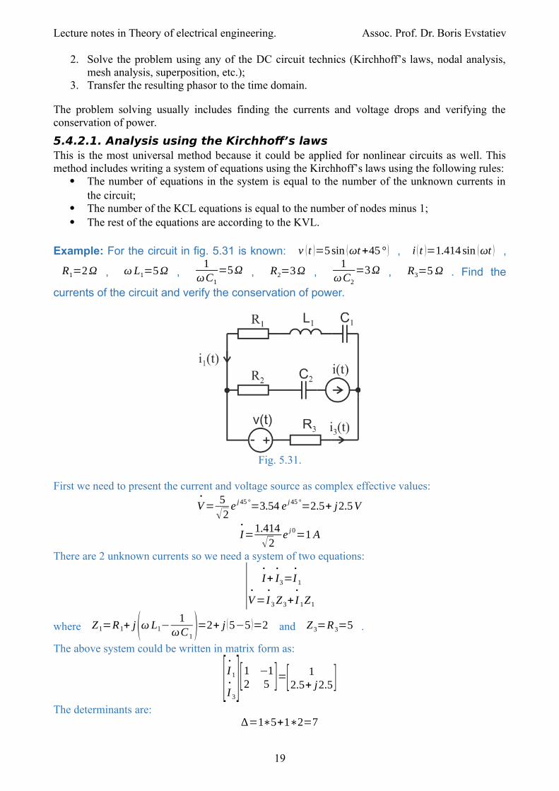
Example: For the circuit in fig. 5.31 is known: v (t )=5sin (ωt+45 ° ) , i (t )=1.414 sin (ωt ) ,
R1=2Ω , ωL1=5Ω , 1
ωC1
=5Ω , R2=3Ω , 1
ωC2
=3Ω , R3=5 Ω . Find the
currents of the circuit and verify the conservation of power.
Fig. 5.31.
First we need to present the current and voltage source as complex effective values:
V•
=5√2
e j45 °=3.54 e j45 °=2.5+ j2.5V
I•
=1.414√2
e j0=1 A
There are 2 unknown currents so we need a system of two equations:
| I•
+ I•
3=I•
1
V•
=I•
3Z3+ I•
1Z1
where Z1=R1+ j(ωL1−1
ωC1)=2+ j (5−5 )=2 and Z3=R3=5 .
The above system could be written in matrix form as:
[I•
1
I•
3][1 −12 5 ]=[ 1
2.5+ j2.5]The determinants are:
∆=1∗5+1∗2=7
19
Lecture notes in Theory of electrical engineering. Assoc. Prof. Dr. Boris Evstatiev
∆1=5+2.5+ j 2.5=7.5+ j 2.5∆3=2.5+ j 2.5−2=0.5+ j2.5
The solution is:
I•
1=∆1
∆=
7.5+ j2.57
=1.07+ j 0.36=1.13 e j18.6°
I•
3=∆3
∆=
0.5+ j 2.57
=0.07+ j 0.36=0.37 e j79 °
In sinusoidal form the currents are:i1 (t )=1.6 sin (ωt+18.6 ° )
i3 (t )=0.52 sin (ωt+79 ° )
Next we need to verify the conservation of power but first we need to find out the voltage drop
V•
I on the current source. We could do that with a KVL for a loop through the current source:
V•
=I•
3Z3+V•
I−I•
Z2
where Z2=R2− j1
ωC2
=3− j 3 .
Then the voltage drop V•
I is:
V•
I=V•
+ I•
Z2−I•
3Z3=2.5+ j 2.5+1. (3− j3 )−5. (0.07+ j 0.36 )=5.15− j2.3The power of the sources is:
S•
SRC=V•
I*
3+V•
I I*
=(2.5+ j2.5 ) (0.07− j 0.36 )+(5.15− j 2.3 ) (1 )==0.175− j 0.9+ j 0.175+0.9+5.15− j2.3=6.225− j3.025VA
The power of the consumers is:
S•
CONS=I 12. Z1+ I 2. Z2+ I 3
2 . Z3=1.132.2+12 . (3− j 3 )+0.372.5=2.55+3− j3+0.685=6.235− j 3VA
It can be seen that S•
SRC ≈S•
CONS. The results do not much perfectly because of round ups.
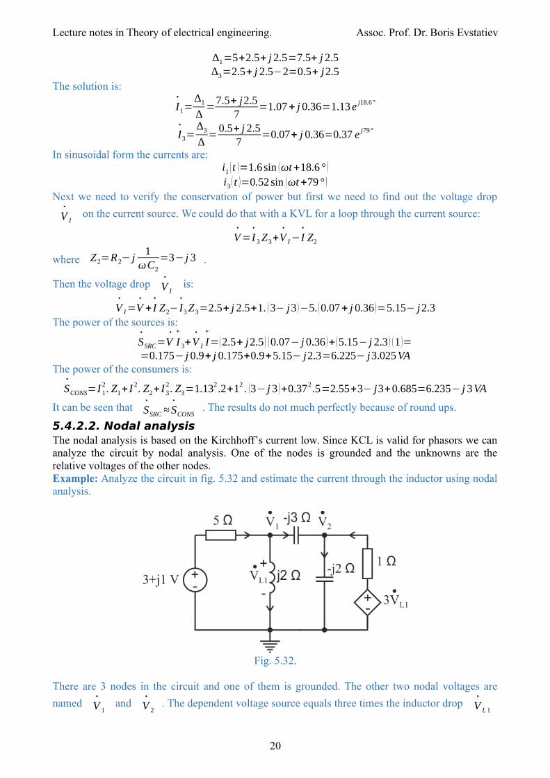
5.4.2.2. Nodal analysisThe nodal analysis is based on the Kirchhoff’s current low. Since KCL is valid for phasors we cananalyze the circuit by nodal analysis. One of the nodes is grounded and the unknowns are therelative voltages of the other nodes.Example: Analyze the circuit in fig. 5.32 and estimate the current through the inductor using nodalanalysis.
Fig. 5.32.
There are 3 nodes in the circuit and one of them is grounded. The other two nodal voltages are
named V•
1 and V
•
2. The dependent voltage source equals three times the inductor drop V
•
L 1
20
Lecture notes in Theory of electrical engineering. Assoc. Prof. Dr. Boris Evstatiev
or:
3V•
L 1=3V•
1
We write two equations based on the KCL for nodes 1 and 2:
|3+ j 1−V
•
1
5=
V•
1−V•
2
− j3+V•
1
j2
V•
1−V•
2
− j3+
3V•
1−V•
2
1=
V•
2
− j2
→|3+ j1
5=V
•
1( 15 +1j2
+1
− j3 )+V•
21j 3
0=V•
1( 1− j3
+3)+V•
2( 1j 3
−1+1j 2 )
Then we write the it in matrix form and estimate the determinants:
[V•
1
V•
2] [0.2− j 0.167 j0.33
3+ j 0.33 −1− j 0.83]=[0.6+ j 0.20 ]
∆=(0.2− j 0.167 ) (−1− j 0.83 )−( j0.33 ) (3+ j0.33 )=−0.229− j0.99∆1=(0.6+ j0.2 ) (−1− j 0.83 )=−0.434− j0.698∆2=−(0.6+ j 0.2 ) (3+ j 0.33 )=−1.734− j 0.798
Then the node voltages are:
V•
1=∆1
∆=
−0.434− j 0.698−0.229− j0.99
=0.766− j 0.261
V•
2=∆2
∆=
−1.734− j0.798−0.229− j0.99
=1.15− j1.49
And the complex current through the inductor is:
I•
L1=V•
1
j2=
0.766− j 0.261j 2
=−0.131− j 0.383
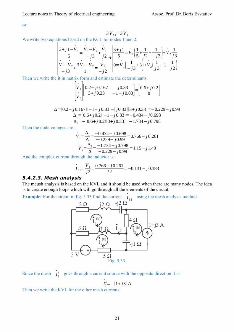
5.4.2.3. Mesh analysisThe meush analysis is based on the KVL and it should be used when there are many nodes. The ideais to create enough loops which will go through all the elements of the circuit.
Example: For the circuit in fig. 5.33 find the current I•
L2 using the mesh analysis method.
Fig. 5.33.
Since the mesh I•
2k goes through a current source with the opposite direction it is:
I•
2k=−(1+ j3 ) A
Then we write the KVL for the other mesh currents:
21
Lecture notes in Theory of electrical engineering. Assoc. Prof. Dr. Boris Evstatiev
|0=I•
1k (2+ j2− j2 )+4 (I
•
1k+1+ j 3)+(3+ j1 )( I
•
2k−I
•
3k)
−5=5 I•
3k+(3+ j1 )( I
•
3k−I
•
1k)− j1( I
•
3k+1+ j3)
or
| −4− j12=I•
1k (2+4+3+ j 1 )−I
•
3k (3+ j 1 )
−5+ j 1−3=−I•
1k (3+ j 1 )+ I
•
3k (5+3+ j1− j 1 )
The above equations can be written in matrix form:
[I•
1k
I•
3k ][ 9+ j1 −(3+ j1 )
−(3+ j1 ) 8 ]=[−4− j12−8+ j 1 ]
The determinants are:∆=72+ j 8−8− j6=64+ j 2
∆1=(−4− j 12 ) (8 )+ (3+ j 1 ) (−8+ j1 )=−57− j101∆3=(9+ j1 ) (−8+ j 1 )−( 4+ j12 ) (3+ j 1 )=−73− j39
And the mesh currents are:
I•
1k=
∆1
∆=
−57+ j10164+ j 2
=−0.939− j 1.549
I•
3k=
∆3
∆=
−73+ j3964+ j 2
=−1.159− j 0.573
And the solution for I•
L2 is:
I•
L2=I•
1k−I
•
3k=−0.939− j1.549+1.159+ j0.573=0.22− j0.976
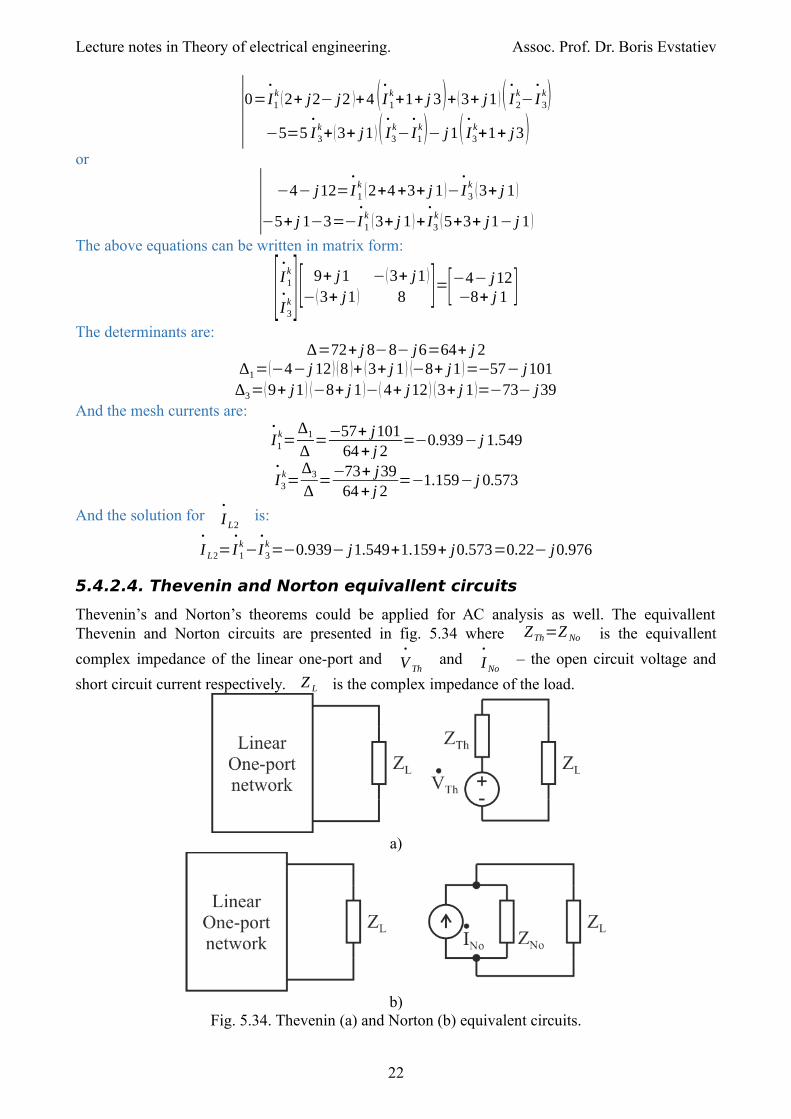
5.4.2.4. Thevenin and Norton equivallent circuits
Thevenin’s and Norton’s theorems could be applied for AC analysis as well. The equivallentThevenin and Norton circuits are presented in fig. 5.34 where ZTh=Z No is the equivallent
complex impedance of the linear one-port and V•
Th and I
•
No – the open circuit voltage and
short circuit current respectively. Z L is the complex impedance of the load.
a)
b)Fig. 5.34. Thevenin (a) and Norton (b) equivalent circuits.
22
Lecture notes in Theory of electrical engineering. Assoc. Prof. Dr. Boris Evstatiev
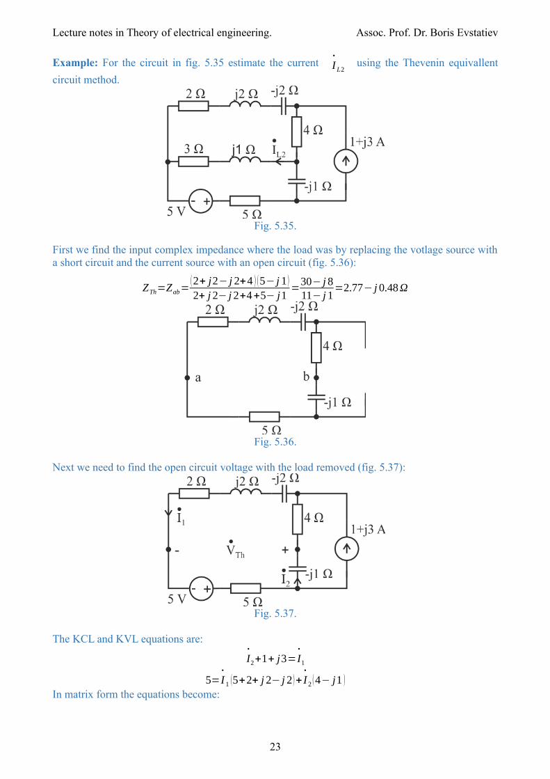
Example: For the circuit in fig. 5.35 estimate the current I•
L2 using the Thevenin equivallent
circuit method.
Fig. 5.35.
First we find the input complex impedance where the load was by replacing the votlage source witha short circuit and the current source with an open circuit (fig. 5.36):
ZTh=Zab=(2+ j2− j 2+4 ) (5− j 1 )
2+ j 2− j 2+4+5− j1=
30− j 811− j 1
=2.77− j 0.48Ω
Fig. 5.36.
Next we need to find the open circuit voltage with the load removed (fig. 5.37):
Fig. 5.37.
The KCL and KVL equations are:
I•
2+1+ j3=I•
1
5=I•
1 (5+2+ j 2− j 2 )+ I•
2 (4− j1 )
In matrix form the equations become:
23
Lecture notes in Theory of electrical engineering. Assoc. Prof. Dr. Boris Evstatiev
[I•
1
I•
2][1 −17 4− j1]=[1+ j 3
5 ]The determinants are:
∆=4− j1+7=11− j 1∆1=4− j1+ j 12+3+5=12+ j 11
∆2=5−7− j21=−2− j 21And the currents are:
I•
1=∆1
∆=
12+ j1111− j 1
=0.992+ j1.09
I•
2=∆2
∆=
−2+ j 2111− j1
=−0.008− j1.91
Then the open circuit voltage is:
5= (0.992+ j1.09 )5+(−0.008− j 1.91 ) (− j 1 )+V•
Th
→V•
Th=5−4.96− j 5.45−0.008 j+1.91=1.95− j 5.46Then the load current in the equivallent Thevenin circuit is:
I•
L2=V•
Th
ZTh+Z Load
=1.95− j 5.46
2.77− j0.48+3+ j 1=0.25− j0.97 A
References
1. Alexander Ch., Sadiku M. Fundamentals of electric circuits. Fifth edition. McGraw-Hill. 2013.Chapter 9, 10, 11.2. http://www.electronics-tutorials.ws/category/accircuits
24