New York Journal of Mathematics On the singular values and ...

SINGULAR VALUES OF LARGE NON-CENTRAL RANDOM MATRICES
W LODEK BRYC AND JACK W. SILVERSTEIN
Abstract. We study largest singular values of large random matrices, each with mean of a fixed rankK. Our main result is a limit theorem as the number of rows and columns approach infinity, while their
ratio approaches a positive constant. It provides a decomposition of the largest K singular values into
the deterministic rate of growth, random centered fluctuations given as explicit linear combinations of theentries of the matrix, and a term negligible in probability. We use this representation to establish asymptotic
normality of the largest singular values for random matrices with means that have block structure. We also
deduce asymptotic normality for the largest eigenvalues of the normalized covariance matrix arising in amodel of population genetics.
1. Introduction
Finite rank perturbations of random matrices have been studied by numerous authors, starting with[Lang, 1964], [Furedi and Komlos, 1981]. This paper can be viewed as an extension of work done in [Silverstein, 1994]which describes the limiting behavior of the largest singular value, λ1, of the M ×N random matrix D(N),consisting of i.i.d. random variables with common mean µ > 0, and M/N → c as N → ∞. Immediateresults are obtained using known properties on the spectral behavior of centered matrices. Indeed, expressD(N) in the form
(1.1) D(N) = C(N) + µ1M1∗N
where C(N) is an M ×N matrix containing of i.i.d. mean 0 random variables having variance σ2 and finitefourth moment, and 1k is the k dimensional vector consisting of 1’s (∗ denotes transpose). When the entriesof C(N) come from the first M rows and N columns of a doubly infinite array of random variables, then itis known ([Yin et al., 1988]) that the largest singular value of 1√
NC converges a.s. to σ(1 +
√c) as N →∞.
Noticing that the sole positive singular value of µ1M1∗N is µ√MN , and using the fact that (see for example
[Stewart and Sun, 1990])
|λ1 − µ√MN | ≤ ‖C‖,
(‖ · ‖ denoting spectral norm on rectangular matrices) we have that almost surely, for all N
λ1 = µ√MN +O(
√N).
From just considering the sizes of the largest singular values of C(N) and µ1M1∗N one can take the view thatDN is a perturbation of a rank one matrix.
A result in [Silverstein, 1994] reveals that the difference between λ1 and µ√MN is smaller than O(
√N).
It is shown that
(1.2) λ1 = µ√MN +
1
2
σ2
µ
(√M
N+
√N
M
)+
1√MN
1MC(N)1∗N +1√MZN ,
where ZN is tight (i.e. stochastically bounded). Notice that the third term converges in distribution toan N(0, σ2) random variable.
This paper generalizes the result in [Silverstein, 1994] by both increasing the rank of the second term onthe right of (1.1) and relaxing the assumptions on the entries of C. The goal is to cover the setting that ismotivated by applications to population biology [Patterson et al., 2006], [Bryc et al., 2013], see also Section3.3.
2010 Mathematics Subject Classification. Primary 60B10; 15A18; Secondary 92D10.
Key words and phrases. non-central random matrices; singular values; asymptotic normality.
1

2 W LODEK BRYC AND JACK W. SILVERSTEIN
We use the following notation. We write A ∈MM×N to indicate the dimensions of a real matrix A, andwe denote by A∗ its transpose; [A]r,s denotes the (r, s) entry of matrix A. Id is the d × d identity matrix.
We use the spectral norm ‖A‖ = supx:‖x‖=1 ‖Ax‖ and occasionally the Frobenius norm ‖A‖F =√
trAA∗.Recall that for an M ×N matrix we have
(1.3) ‖A‖ ≤ ‖A‖F .Vectors are denoted by lower case boldface letters like x and treated as column matrices so that the Euclideanlength is ‖x‖2 = x∗x.
Throughout the paper, we use the same letter C to denote various positive non-random constants that donot depend on N . The phrase ”... holds for all N large enough” always means that there exists a non-randomN0 such that ”...” holds for all N > N0.
We fix K ∈ N and a sequence of integers M = M (N) such that
(1.4) limN→∞
M/N = c > 0.
We consider a sequence of vectors f(N)1 , . . . f
(N)K ∈ RM and g
(N)1 , . . .g
(N)K ∈ RN and introduce matrices
F = F(N) ∈MM×K , G = G(N) ∈MN×K , and R0 = R(N)0 ∈MK×K with:
(1.5) F = [f(N)1 , . . . , f
(N)K ], G = [g
(N)1 , . . . ,g
(N)K ], and R0 = G∗G = [g∗rgs].
Our first set of assumptions deals with properties of the deterministic perturbation.
Assumption 1.1. We assume the following
(i) Vectors f(N)1 , . . . f
(N)K ∈ RM are orthonormal.
(ii)
(1.6) 1MNR
(N)0 → Q.
(iii) The eigenvalues γ1, . . . , γK of matrix Q are distinct and strictly positive.
We shall write the eigenvalues of Q in decreasing order, γ1 > γ2 > · · · > γK > 0, and we denote thecorresponding unit eigenvectors by v1, . . . ,vK . Note that ‖G‖ ≤ ‖R0‖1/2 ≤ 2
√MN‖Q‖ for large enough
N .Our second set of assumptions deals with randomness.
Assumption 1.2. Let C = C(N) be an M ×N random matrix with real independent entries [C]i,j = Xi,j .(The distributions of the entries may differ, and may depend on N .) We assume that E(Xi,j) = 0 and thatthere exists a constant C such that
(1.7) E(X4i,j) ≤ C.
In particular, the variances
σ2i,j = E(X2
i,j)
are uniformly bounded.We are interested in the asymptotic behavior of the K largest singular values λ1 ≥ λ2 ≥ · · · ≥ λK of the
sequence of noncentered random M ×N matrices
(1.8) D(N) = D = C + FG∗ = C +
K∑s=1
fsg∗s .
(Recall that vectors fs = f(N)s and gs = g
(N)s also depend on N .)
Our main result represents each singular value λr as a sum of four terms, which represent the rate ofgrowth, random centered fluctuation, deterministic shift, and a term negligible in probability. To state thisresult we need additional notation.
The rate of growth is determined by the eigenvalues ρ(N)1 ≥ ρ
(N)2 ≥ ρ
(N)K ≥ 0 of the deterministic matrix
R0 defined in (1.5).The random centered fluctuation term for the r-th singular value λr is
(1.9) Z(N)r =
1√γr
v∗rZ0vr,

SINGULAR VALUES OF RANDOM MATRICES 3
where Z0 is a random centered K ×K matrix given by
(1.10) Z0 =1√MN
G∗C∗F.
Note that Z0 implicitly depends on N also through fr = f(N)r and gs = g
(N)s .
The expression for the constant shift depends on the variances of the entries of C. To write the expressionwe introduce a diagonal N ×N matrix ∆R = E(C∗C)/M and a diagonal M ×M matrix ∆S = E(CC∗)/N .The diagonal entries of these matrices are
[∆R]j,j =1
M
M∑i=1
σ2i,j , [∆S ]i,i =
1
N
N∑j=1
σ2i,j .
Let Σr = Σ(N)R and ΣS = Σ
(N)S be deterministic K ×K matrices given by
(1.11) ΣR = G∗∆RG = [g∗r∆Rgs]
and
(1.12) ΣS = F∗∆SF = [f∗r∆Sfs].
Define
(1.13) m(N)r =
1
2√cγr
v∗r
(c
γrMNΣR + ΣS
)vr.
Theorem 1.1. With the above notation, there exist ε(N)1 → 0, . . . ε
(N)K → 0 in probability such that for
1 ≤ r ≤ K we have
(1.14) λr =
√ρ
(N)r + Z(N)
r +m(N)r + ε(N)
r .
Expression (1.14) is less precise than (1.2) (where ε(N) = ZN/√M → 0 at known rate), but it is strong
enough to establish asymptotic normality under appropriate additional conditions. Such applications areworked out in Section 3.
We remark that the case when eigenvalues of Q have multiplicity greater than 1, or are zero, are notcovered by our approach, and this is left for further study at a later time.
2. Proof of Theorem 1.1
Throughout the proof, we assume that all our random variables are defined on a single probability space(Ω,F ,P). In the initial parts of the proof we will be working on subsets ΩN ⊂ Ω such that P(ΩN )→ 1.
2.1. Singular value criterion. In this section, we fix r ∈ 1, . . . ,K and let λ = λr. For ‖C‖2 < λ2,matrices IM − 1
λ2 CC∗ and IN − 1λ2 C∗C are invertible, so we consider the following K ×K matrices:
Z =1
λG∗(IN − 1
λ2 C∗C)−1
C∗F ,(2.1)
S = F∗(IM − 1
λ2 CC∗)−1
F ,(2.2)
R = G∗(IN − 1
λ2 C∗C)−1
G .(2.3)
(These auxiliary random matrices depend on N and λ, and are well defined only on a subset of the probabilityspace Ω.)
Lemma 2.1. If ‖C‖2 < λ2/2 then
(2.4) det
[Z− λIK R
S Z∗ − λIK
]= 0.
4 W LODEK BRYC AND JACK W. SILVERSTEIN
Proof. The starting point is the singular value decomposition D = UΛV∗. We choose the r-th columnsu ∈ RM of U and v ∈ RN of V that correspond to the singular value λ = λr. Then (1.8) gives
Cv +
K∑s=1
(g∗sv)fs = λu ,(2.5)
C∗u +
K∑s=1
(f∗su)gs = λv .(2.6)
Multiplying from the left by C∗ or C we get
C∗Cv +
K∑s=1
(g∗sv)C∗fs = λC∗u,(2.7)
CC∗u +
K∑s=1
(f∗su)Cgs = λCv.(2.8)
Using (2.5) and (2.6) to the expressions on the right, we get
C∗Cv +
K∑s=1
(g∗sv)C∗fs = λ2v − λK∑s=1
(f∗su)gs ,(2.9)
CC∗u +
K∑s=1
(f∗su)Cgs = λ2u− λK∑s=1
(g∗sv)fs .(2.10)
which we rewrite as
λ2v −C∗Cv =
K∑s=1
(g∗sv)C∗fs + λ
K∑s=1
(f∗su)gs ,(2.11)
λ2u−CC∗u = λ
K∑s=1
(g∗sv)fs +
K∑s=1
(f∗su)Cgs .(2.12)
This gives
v =1
λ2
K∑s=1
(g∗sv)(IN − 1
λ2 C∗C)−1
C∗fs +1
λ
K∑s=1
(f∗su)(IN − 1
λ2 C∗C)−1
gs ,(2.13)
u =1
λ
K∑s=1
(g∗sv)(IM − 1
λ2 CC∗)−1
fs +1
λ2
K∑s=1
(f∗su)(IM − 1
λ2 CC∗)−1
Cgs .(2.14)
Notice that since u,v are unit vectors, some among the 2K the numbers (f∗1 u), . . . , (f∗Ku), (g∗1v), . . . , (g∗Kv)must be non-zero. Since for 1 ≤ t ≤ K we have
(g∗tv) =1
λ2
K∑s=1
(g∗sv)g∗t(IN − 1
λ2 C∗C)−1
C∗fs +1
λ
K∑s=1
(f∗su)g∗t(IN − 1
λ2 C∗C)−1
gs ,(2.15)
(f∗t u) =1
λ
K∑s=1
(g∗sv)f∗t(IM − 1
λ2 CC∗)−1
fs +1
λ2
K∑s=1
(f∗su)f∗t(IM − 1
λ2 CC∗)−1
Cgs ,(2.16)
noting that the entries of Z∗ can be written as
(2.17) [Z∗]s,t =1
λf∗s (IM − 1
λ2 CC∗)−1Cgt .
we see that the block matrix [1λZ 1
λR1λS 1
λZ∗
]has eigenvalue 1. Thus det
[1λZ− IK
1λR
1λS 1
λZ∗ − IK
]= 0 which for λ > 0 is equivalent to (2.4).
SINGULAR VALUES OF RANDOM MATRICES 5
Proposition 2.2 (Singular value criterion). If ‖C‖2 < λ2/4 then S is invertible and
(2.18) det((λIK − Z)S−1(λIK − Z∗)−R
)= 0.
Similar equations that involve a K ×K determinant appear in other papers on rank-K perturbations ofrandom matrices, compare [Tao, 2013, Lemma 2.1 and Remark 2.2]. Note however that in our case λ entersthe equation in a rather complicated way through Z = Z(λ),R = R(λ),S = S(λ). The dependence of thesematrices on N is also suppressed in our notation.
Proof. Note that if ‖C‖2 ≤ λ2/2 then the norms of(IM − 1
λ2 CC∗)−1
and(IN − 1
λ2 C∗C)−1
are bounded
by 2. Indeed, ‖(IM − 1
λ2 CC∗)−1 ‖ ≤
∑∞k=0 ‖(CC∗)k‖/λ2k ≤
∑∞k=0 1/2k. Since
(IM − 1
λ2 CC∗)−1
= IM +1λ2 CC∗
(IM − 1
λ2 CC∗)−1
and vectors f1, . . . , fK are orthonormal, we get F∗F = IK and
(2.19) S− IK =1
λ2F∗C∗C
(IM − 1
λ2 CC∗)−1
F .
Since ‖F‖ = 1 we have
(2.20) ‖S− IK‖ ≤ 2‖C‖2/λ2.
We see that if ‖C‖2 ≤ λ2/4 then ‖S − IK‖ ≤ 1/2, so the inverse S−1 =∑∞k=0(I − S)k exists. For later
citation we also note that
(2.21) ‖S−1‖ ≤ 2.
Since [R Z− λIK
Z∗ − λIK S
]=
[Z− λIK R
S λZ∗ − λIK
]×[
0 IKIK 0
],
we see that (2.4) is equivalent to
det
[R Z− λIK
Z∗ − λIK S
]= 0.
Noting that λ > 0 by assumption, we see that (2.4) holds and gives (2.18), as by Schur’s complement formula
det
[A BC D
]= detD det(A−BD−1C).
2.2. Equation for λr. As was done previously we fix r ∈ 1, . . . ,K, and write λ = λr. For eigenvalues
ρ(N)1 ≥ ρ
(N)2 ≥ ρ
(N)K ≥ 0 of R0, we denote the corresponding orthonormal eigenvectors of R0 by u1 =
u(N)1 , . . . ,uK = u
(N)K ∈ RK . The main step in the proof of Theorem 1.1 is the following expression.
Proposition 2.3. There exists a random sequence ε(N)c → 0 in probability as N →∞ such that
(2.22) λ−√ρ
(N)r =
N
λ+
√ρ
(N)r
u∗rΣSur +2√MN
λ+
√ρ
(N)r
u∗rZ0ur +M
(λ+
√ρ
(N)r )λ2
u∗r(ΣR)ur + ε(N)c .
The proof of Proposition 2.3 is technical and lengthy.
2.2.1. Subset ΩN . With γK+1 := 0, let
(2.23) δ := min1≤s≤K
(γs − γs+1).
Assumption 1.1(iii) says that δ > 0.
Definition 2.1. Let ΩN ⊂ Ω be such that
(2.24) ‖C‖2 ≤ N5/4
and
(2.25) max1≤s≤K
|λ2s − γsMN | ≤ δ
4MN.

6 W LODEK BRYC AND JACK W. SILVERSTEIN
We assume that N is large enough so that ΩN is a non-empty set. In fact, P(ΩN )→ 1, see Lemma 2.4.
We note that (2.25) implies that c√MN ≤ λr ≤ C
√MN with c =
√γr − δ/4 ≥
√γK − δ/4 >
√δ/2 and
C =√γr + δ/4 < 2
√γ1 = 2
√‖Q‖. For later reference we state these bounds explicitly:
(2.26)
√δMN
2≤ λr ≤ 2
√‖Q‖MN.
We also note that inequalities (2.24) and (2.26) imply that
(2.27) ‖C‖2 < λ2K
4
for all N large enough. (That is, for all N > N0 with nonrandom constant N0.) Thus matrices Z, R, S arewell defined on ΩN for large enough N and (2.18) holds.
Lemma 2.4. For 1 ≤ r ≤ K we have λr/√MN → γr in probability. Furthermore, P(ΩN )→ 1 as N →∞.
Proof. As previously, we denote by ρ1 > ρ2 > · · · > ρK the eigenvalues of the K × K matrix R0. Theseeigenvalues are distinct and strictly positive for large enough N ; as before we denote by u1, . . . ,uK the
corresponding orthonormal eigenvectors. Let M × N matrix A = FG∗ =∑Kr=1 frg
∗r . Since A∗A = GG∗
and R0 = G∗G, we that the non-zero singular values of A are distinct and equal to√ρ1 >
√ρ2 > · · · >
√ρK .
From (1.8) we have D−A = C, so by Weil-Mirsky theorem [Stewart and Sun, 1990, page 204, Theorem
4.11], we have a bound |λr −√ρ
(N)r | ≤ ‖C‖ for the differences between the K largest singular values of A
and D. From [Lata la, 2005, Theorem 2] we see that there is a constant C that does not depend on N such
that E‖C‖ ≤ C(√M +
√N). Thus
λr −√ρ
(N)r√
MN→ 0 in probability.
Since ρ(N)r /MN → γr > 0 we see that λr/
√MN → √
γr in probability, proving the first part of theconclusion.
To prove the second part, we use the fact that continuous functions preserve convergence in probability,so λ2
r/(MN)→ γr in probability for 1 ≤ r ≤ K. Thus
P(Ω′N ) ≤ P(‖C‖ > N5/8) +
K∑s=1
P(|λ2s − γsMN | > δMN/4)
≤ C√M +
√N
N5/8+
K∑s=1
P(|λ2s/(MN)− γs| > δ/4)→ 0 as N →∞.
2.2.2. Proof of Proposition 2.3. In view of (2.27), equation (2.18) holds on ΩN if N is large enough. It
implies that there is a (random) unit vector x(N)r = x ∈ RK such that
(λIK − Z)S−1(λIK − Z∗)x = Rx.
Using matrix (1.5), we rewrite this as follows.
(2.28) (λ2IK −R0)x =(λ2(IK − S−1) + λ(ZS−1 + S−1Z∗)− ZS−1Z∗ + (R−R0)
)x.
We now rewrite this equation using the (nonrandom) eigenvalues ρ(N)1 ≥ ρ
(N)2 ≥ ρ
(N)K ≥ 0 and the
corresponding orthonormal eigenvectors u1 = u(N)1 , . . . ,uK = u
(N)K ∈ RK of R0.
Suppressing dependence on r and N in the notation, we insert
x =
K∑t=1
αtut

SINGULAR VALUES OF RANDOM MATRICES 7
into (2.28) and multiply the resulting expression by u∗s from the left. This shows that λr satisfies the followingsystem of K equations
(2.29) (λ2 − ρs)αs = λ2u∗s(IK − S−1)x + λu∗s(ZS−1 + S−1Z∗)x + u∗s(R − R0)x − u∗sZS−1Z∗x,
where 1 ≤ s ≤ K. (Recall that this is a system of highly nonlinear equations as matrices S, Z and R, aswell as coefficients α1, . . . αK , depend implicitly on λ.)
It turns out that for our choice of λ = λr random variable α(N)r is close to its extreme value 1 while the
other coefficients are asymptotically negligible. Since this only holds on ΩN a more precise statement is asfollows.
Lemma 2.5. There exist deterministic constants C and N0 such that for all N > N0 and ω ∈ ΩN we have
(2.30) 1− CN−3/8 ≤ αr ≤ 1
and
(2.31) |αs| ≤ (C/√K − 1)N−3/8 for s 6= r.
Proof. Since∑α2s = 1, inequality (2.30) is a consequence of (2.31). Indeed, α2
r = 1−∑s6=r α
2s ≥ 1−C2N−3/4
and we use elementary inequality√
1− x ≥ 1−√x for 0 ≤ x ≤ 1.
To prove (2.31), we apply (2.29).
From (1.6) by Weil’s theorem we get ρ(N)j /(MN)→ γj . Using (2.23), we choose N large enough so that
|ρs − γsMN | ≤ δMN/4. Then, with s 6= r we get
|λ2 − ρs| = |(λ2 − γrMN) + (γr − γs)MN + (γsMN − ρs)|
≥ |γr − γs|MN − |λ2 − γrMN | − |ρs − γsMN | ≥ (|γr − γs| − δ/2)MN ≥ δ
2MN.
From (2.26) and (2.29) we get
(2.32)δ
2MN |αs| ≤ 4‖Q‖MN‖IK − S−1‖+ 4
√‖Q‖√MN‖Z‖ ‖S−1‖+ ‖R−R0‖+ ‖Z‖2‖S−1‖.
Since IK − S−1 = S−1(S− IK) using (2.21) we get
(2.33) |αs| ≤16‖Q‖δ‖S− IK‖+
16√‖Q‖
δ√MN
‖Z‖+2
δMN‖R−R0‖+
4
δMN‖Z‖2.
We now estimate the norms of the K × K matrices on the right hand side. From (2.20) using (2.24) and(2.26) we get
(2.34) ‖S− IK‖ ≤2‖C‖2
λ2≤ 8N5/4
δMN=
8
δN1/4M−1.
Next, we bound ‖Z‖ using (2.1). Recall that ‖(IN − 1
λ2 C∗C)−1 ‖ ≤ 2 for large enough N . From (1.6)
we have‖G‖ ≤ 2√MN‖Q‖, for large enough N . Using this, (2.24) and (2.26) we get
(2.35) ‖Z‖ ≤ ‖G‖ 2
λ‖C‖ ≤
4√MN‖Q‖λ
N5/8 ≤ 8‖Q‖1/2√δ
N5/8
for large enough N .Next we note that
(2.36) R−R0 =1
λ2G∗C∗C
(IN − 1
λ2 C∗C)−1
G .
Thus (2.36) with bounds (2.26), (2.24) and the above bound on ‖G‖ give us for large enough N
(2.37) ‖R−R0‖ ≤8MN‖Q‖
λ2‖C‖2 ≤ 32‖Q‖
δN5/4.
Putting these bounds into (2.33) we get
|αs| ≤128‖Q‖δ2
N1/4M−1 +128‖Q‖δ√δ
N1/8M−1/2 +64‖Q‖δ2
N1/4M−1 +256‖Q‖δ2
N1/4M−1.
In view of assumption (1.4), this proves (2.31).

8 W LODEK BRYC AND JACK W. SILVERSTEIN
The next step is to use Lemma 2.5 to rewrite the r-th equation in (2.29) to identify the ”contributingterms” and the negligible ”remainder” R which is of lower order than λ on ΩN . We will accomplish this inseveral steps, so we will use the subscripts a, b, c, . . . for bookkeeping purposes.
Define x(r) by
x(r) =∑s6=r
αsus.
We assume that N is large enough so that the conclusion of Lemma 2.5 holds and furthermore thatαr ≥ 1/2. Notice then that
(2.38) ‖x(r)‖ ≤ CN−3/8.
Dividing (2.29) with s = r by αr we get
(2.39) λ2−ρ(N)r = λ2u∗r(IK −S−1)ur + 2λu∗rZS−1ur +u∗r(R−R0)ur−u∗rZS−1Z∗ur +
√MNε(N)
a +R(N)a ,
where
(2.40) ε(N)a =
1
αru∗r(Z0 + Z∗0)x(r)
and
(2.41) R(N)a = λ2 1
αru∗r(IK − S−1)x(r) + λ
1
αru∗r(ZS−1 + S−1Z∗ −
√MN
λ(Z0 + Z∗0))x(r)
+1
αru∗r(R−R0)x(r) −
1
αru∗rZS−1Z∗x(r) .
Here we slightly simplified the equation noting that since S is symmetric, u∗rZS−1ur = u∗rS−1Z∗ur.
Our first task is to derive a deterministic bound for R(N)a on ΩN .
Lemma 2.6. There exist non-random constants C and N0 such that on ΩN for N > N0 we have
(2.42) |R(N)a | ≤ CN7/8.
Proof. The constant will be given by a complicated expression that will appear at the end of the proof.Within the proof, C denotes the constant from Lemma 2.5.
Notice that
(2.43) Z−√MN
λZ0 =
1
λ3G∗C∗C
(IN − 1
λ2 C∗C)−1
C∗F ,
so for large enough N we get
(2.44) ‖Z−√MN
λZ0‖ ≤
4
λ3
√MN‖Q‖‖C‖3 ≤ 32‖Q‖1/2
δ3/2N7/8M−1.
Recall (2.21)and recall that N large enough so that αr > 1/2. Using (2.38) and writing ZS−1 = ZS−1(S − IK) + Z
we get
(2.45) |R(N)a | ≤ 4Cλ2N−3/8‖S− IK‖+ 8CλN−3/8‖Z‖‖S− IK‖+ 4CλN−3/8‖Z−
√MN
λZ0‖
+ 2CN−3/8‖R−R0‖+ 2CN−3/8‖Z‖2
≤ 128C‖Q‖δ
N7/8 +1024C‖Q‖
δ3/2M−1/2N +
256C‖Q‖δ3/2
M−1/2N
+64C‖Q‖
δN7/8 +
128C‖Q‖δ
N7/8.
(Here we used (2.34), (2.35), then (2.44), (2.37) and (2.35) again.) This concludes the proof.

SINGULAR VALUES OF RANDOM MATRICES 9
Lemma 2.7. For every η > 0, we have
(2.46) limN→∞
P(∣∣∣ε(N)
a
∣∣∣ > η∩ ΩN
)= 0.
Proof. We first verify that each entry of the matrix N−3/8Z0, which is well defined on Ω, converges inprobability to 0. To do so, we bound the second moment of random variable ξ = f∗rCgs. Since the entriesof C are independent and centered random variables,
(2.47) Eξ2 =
M∑i=1
N∑j=1
[fr]2iσ
2i,j [gs]
2j ≤ sup
i,jσ2i,j‖gr‖2 ≤ CMN.
Thus, see (1.10), each entry of matrix Z0 has bounded second moment, so
ζN := N−3/8 maxs|u∗r(Z0 + Z∗0)us| → 0 in probability.
To end the proof we note that by (2.31), for large enough N we have∣∣∣ε(N)a
∣∣∣ ≤ 2CKζN on ΩN , so
P(∣∣∣ε(N)
a
∣∣∣ > η∩ ΩN
)≤ P
(|ζN | > η
2CK ∩ ΩN)≤ P
(|ζN | > η
CK
)→ 0.
Using the identity
(2.48) I− S−1 = (S− I)− (S− I)2S−1
to the first term we rewrite (2.39) as
(2.49) λ2 − ρ(N)r = λ2u∗r(S− IK)ur + 2λu∗rZur + u∗r(R−R0)ur − u∗rZZ∗ur +R(N)
b +√MNε(N)
a +R(N)a ,
with
(2.50) R(N)b = −λ2u∗r(S− IK)2S−1ur + 2λu∗rZ(IK − S)S−1ur − u∗rZ(IK − S)S−1Z∗ur .
Lemma 2.8. There exist non-random constants C and N0 such that on ΩN for N > N0 we have
(2.51) |R(N)b | ≤ CN7/8.
Proof. Using (2.26) and previous norm estimates (2.34) and (2.35), we get
|R(N)b | ≤ 2λ2‖S− IK‖2 + 4λ‖Z‖‖S− IK‖+ 2‖Z‖2‖S− IK‖
≤ 512‖Q‖δ2
N3/2M−1 +512‖Q‖δ3/2
N11/8M−1/2 +1024|Q‖
δ2N3/2M−1.
This ends the proof.
Define K ×K random matrices
(2.52) R1 = G∗C∗CG
and
(2.53) S1 = F∗CC∗F .
Recall that E(R1) = MΣR and E(S1) = NΣS , see (1.11) and (1.12).
Lemma 2.9. There exist non-random constants C and N0 such that on ΩN for N > N0 we have
(2.54) ‖S− IK −1
λ2S1‖ ≤ CN−3/2
and
(2.55) ‖R−R0 − 1λ2 R1‖ ≤ CN1/2.

10 W LODEK BRYC AND JACK W. SILVERSTEIN
Proof. Notice that
(2.56) S− IK −1
λ2S1 =
1
λ4F∗(CC∗)2(IM − 1
λ2 CC∗)−1F.
For large enough N (so that (2.24) and (2.26) hold), this gives
‖S− IK −1
λ2S1‖ ≤
2
λ4‖C‖4 ≤ 32
δ2M−2N1/2.
Similarly, since
(2.57) R−R0 − 1λ2 R1 =
1
λ4G∗(C∗C)2
(IN − 1
λ2 C∗C)−1
G
for large enough N , we get
‖R−R0 − 1λ2 R1‖ ≤ max
r,s
2
λ4‖G‖2‖C‖4 ≤ 128‖Q‖
δ2M−1N3/2.
We now rewrite (2.49) as follows.
(2.58) λ2 − ρ(N)r
= u∗r(S1)ur + 2√MNu∗rZ0ur +
1
λ2u∗r(R1)ur −
MN
λ2u∗rZ0Z
∗0ur +R(N)
c +R(N)b +
√MNε(N)
a +R(N)a ,
where
(2.59) R(N)c
= u∗r
(λ2(S− IK −
1
λ2S1) + 2(λZ−
√MNZ0) + (R−R0 −
1
λ2R1) + (
MN
λ2Z0Z
∗0 − ZZ∗)
)ur .
Lemma 2.10. There exist non-random constants C and N0 such that on ΩN for N > N0 we have
|R(N)c | ≤ CN7/8.
Proof. As in the proof of Lemma 2.6, the final constant C can be read out from the bound at the end of theproof. In the proof, C is a constant from Lemma 2.9. By triangle inequality, Lemma 2.9, (2.44) and (2.35),we have
(2.60) |R(N)c | ≤ λ2‖S− IK −
1
λ2S1‖+ 2‖λZ−
√MNZ0‖
+ ‖R−R0 −1
λ2R1‖+ ‖Z−
√MN
λZ0‖(‖Z‖+
√MN
λ‖Z0‖)
≤ 4C‖Q‖MN−1/2 +128‖Q‖δ3/2
M−1/2N11/8 + CN1/2 +256‖Q‖δ2
M−1N3/2 +128‖Q‖δ3/2
M−1N3/2.
(Here we used the bound ‖Z0‖ ≤ 2‖Q‖1/2N5/8, which is derived similarly to (2.35).)
The following holds on Ω. (Recall that expressions (2.53), (1.10) and (2.52) are well defined on Ω.)
Proposition 2.11. There exists a random sequence ε(N)b → 0 in probability as N →∞ such that
(2.61) λ−√ρ
(N)r =
1
λ+
√ρ
(N)r
u∗r(S1)ur +2√MN
λ+
√ρ
(N)r
u∗rZ0ur +1
(λ+
√ρ
(N)r )λ2
u∗r(R1)ur + ε(N)b .
Proof. Let
ε(N)b =
1
λ+√ρ(N)r
(−MN
λ2 u∗rZ0Z∗0ur +R(N)
c +R(N)b +
√MNε
(N)a +R(N)
a
)on ΩN ,
λ−√ρ
(N)r − 1
λ+√ρ(N)r
u∗r(S1)ur − 2λ
λ+√ρ(N)r
u∗rZ0ur − 1
(λ+√ρ(N)r )λ2
u∗r(R1)ur otherwise.
By Lemma 2.4 we have P(Ω′N )→ 0, so it is enough to show that given η > 0 we have P(|ε(N)b | > 5η∩ΩN )→
0 as N →∞. Since the event |ξ1 + · · ·+ ξ5| > 5η is included in the union of events |ξ1| > η, . . . , |ξ5| > η, in
SINGULAR VALUES OF RANDOM MATRICES 11
view of Lemmas 2.6, 2.8, 2.10, and Lemma 2.7 (recalling that expressions√MN/(λ+
√ρ
(N)r ) and MN/λ2
are bounded by a non-random constant on ΩN , see (2.26)) we only need to verify that
P
u∗rZ0Z∗0ur
λ+
√ρ
(N)r
> η
∩ ΩN
≤ Pu∗rZ0Z
∗0ur√
ρ(N)r
> η
→ 0 as N →∞.
Since for large enough N , we have ρ(N)r ≥ δMN , convergence follows from
(2.62) Eu∗rZ0Z∗0ur ≤ E‖Z0‖2 ≤ E‖Z0‖2F ≤ K2C,
where C is a constant from (2.47).
Proof of Proposition 2.3. Recall that ES1 = NΣS and ER1 = MΣR. So expression (2.22) differs from(2.61) only by two terms:
1
λ+
√ρ
(N)r
u∗r(S1 − ES1)ur
and1
(λ+
√ρ
(N)r )λ2
u∗r(R1 − ER1)ur.
Since ρ(N)r /(MN) → γr > 0 and by Lemma 2.4 we have λ/
√MN → √γr in probability, to end the proof
we show that 1N ‖S1 −ES1‖F → 0 and 1
N3 ‖R1 −ER1‖F → 0 in probability. To do so, we bound the secondmoments of the entries of the matrices. Recalling (2.53), we have
f∗r (CC∗ − E(CC∗))fs =
N∑k=1
∑i 6=j
[fr]iXi,kXj,k[fs]j +
N∑k=1
M∑i=1
[fr]i(X2i,k − σ2
i,k)[fs]i = AN + BN (say).
By independence, we have
E(A2N ) =
N∑k=1
∑i6=j
[fr]2i [fs]
2jσ
2i,kσ
2j,k ≤ C
N∑k=1
N∑i=1
N∑j=1
[fr]2i [fs]
2j ≤ CN.
Next,
E(B2N ) =
N∑k=1
M∑i=1
[fr]2i [fs]
2iE(X2
i,k − σ2i,k)2 ≤ NC
√√√√ M∑i=1
[fr]4i
√√√√ M∑i=1
[fs]4i ≤ CN.
This shows that (with a different C) we have E |f∗r (CC∗ − E(CC∗)fs)|2 ≤ CN and hence 1N ‖S1−ES1‖F → 0
in mean square and in probability.Similarly, recalling (2.52) we have
g∗r(C∗C − E(C∗C))gs =
M∑k=1
∑i 6=j
[gr]i[gs]jXk,iXk,j +
M∑k=1
N∑i=1
[gr]i[gs]i(X2k,i − σ2
k,i) = AN + BN (say).
Using independence of entries again, we get
E(A2N ) =
M∑k=1
∑i6=j
[gr]2i [gs]
2jσ
2k,iσ
2k,j ≤ CM‖gs‖2‖gr‖2 ≤ C‖Q‖4FM3N2
for large enough N . Similarly,
E(B2N ) =
M∑k=1
N∑i=1
[gr]2i [gs]
2iE(X2
k,i − σ2k,i)
2 ≤ CM‖gr‖2‖gs‖2 ≤ C‖Q‖4FM3N2.
This shows that (with a different C) we have E |g∗r(C∗C− E(C∗C))gs|2 ≤ CN5 and hence 1N3 ‖R1 −
ER1‖F → 0 in mean square and in probability.
12 W LODEK BRYC AND JACK W. SILVERSTEIN
2.2.3. Conclusion of proof of Theorem 1.1. Theorem 1.1 is essentially a combination of (2.22), convergencein probability from Lemma 2.4, and convergence of eigenvectors. For the later, without loss of generalitywe may assume that the first non-zero component of vr is positive. After choosing the appropriate sign,
without loss of generality we may assume that the same component of u(N)r is non-negative for all N . Since
by assumption eigenspaces of R0 are one-dimensional for large enough N , therefore
(2.63) u(N)r → v as N →∞.
Proof of Theorem 1.1. We need to do a couple more approximations to the right hand side of (2.22). FromLemma 2.4 and (2.63) we see that
N
λ+
√ρ
(N)r
u∗rΣSur ∼N
2√γr√MN
v∗rΣSvr ∼√N/M
2√γr
v∗rΣSvr
in probability. Similarly,
M
(λ+
√ρ
(N)r )λ2
u∗r(ΣR)ur ∼√M/N
2√γr
1
γrMNv∗r(ΣR)vr .
Finally, since by (2.47) the entries of Z0 are stochastically bounded, (2.63) gives
2√MN
λ+
√ρ
(N)r
u∗rZ0ur ∼1√γr
v∗rZ0vr .
3. Asymptotic normality of singular values
In this section we apply Theorem 1.1 to deduce asymptotic normality. To reduce technicalities involved,we begin with the simplest case of mean with rank 1. An example with mean of rank 2 is worked out inSection 3.2. A more involved application to population biology appears in Section 3.3. We use simulationsto illustrate these results.
3.1. Rank 1 perturbation. The following is closely related to [Silverstein, 1994, Theorem 1.3] that wasmentioned in the introduction.
Proposition 3.1. Fix an infinite sequence µj such that the limit γ = limN→∞1N
∑Nj=1 µ
2j exists. Consider
the case K = 1, and assume that entries of D are independent, with the same mean µj in the j-th column,the same variance σ2, and uniformly bounded fourth moments. For the largest singular value λ of D, we
have λ−√M(∑N
j=1 µ2j
)1/2
⇒ Z where Z is normal with mean σ2
2√γ (√c+ 1/
√c) and variance σ2.
Proof. In this setting (1.8) holds with f = M−1/2[1, . . . , 1]∗, g =√M [µ1, . . . , µN ]∗. We get ρ1 = M
∑Nj=1 µ
2j ,
γ1 = γ, ΣR = σ2M∑Nj=1 µ
2j , ΣS = σ2, and
Z0 =1√MN
M∑i=1
N∑j=1
Xi,jµj , so (1.9) gives Z1 =1√MNγ
M∑i=1
N∑j=1
Xi,jµj .
Thus, with ε(N) → 0 in probability, the largest singular value of D can be written as
λ =√M
N∑j=1
µ2j
1/2
+σ2(√c+ 1/
√c)
2√γ
+1√MNγ
M∑i=1
N∑j=1
Xi,jµj + ε(N),
where ε(N) → 0 in probability.In particular,
Var(Z1) =σ2
γ
1
N
N∑j=1
µ2j → σ2

SINGULAR VALUES OF RANDOM MATRICES 13
and the sum of the fourth moments of the terms in Z1 is
1
M2N2γ2
M∑i=1
N∑j=1
µ4jEX
4i,j ≤
C
M
1
N
N∑j=1
µ2j
2
→ 0.
So Z1 is asymptotically normal by Lyapunov’s theorem [Billingsley, 2012, Theorem 27.3].
3.2. Block matrices. Consider (2M)× (2N) block matrices
D =
[A1 A2
A3 A4
],
where A1, . . . ,A4 are independent random M ×N matrices. We assume that the entries of Aj are indepen-dent real identically distributed random variables with mean µj , variance σ2
j and with finite fourth moment.Then E(D) = f1g
∗1 + f2g
∗2 with orthonormal
[f1]i =
1/√M for 1 ≤ i ≤M
0 for M + 1 ≤ i ≤ 2M
[f2]i =
0 for 1 ≤ i ≤M1/√M for M + 1 ≤ i ≤ 2M
and with
[g1]j =
√Mµ1 for 1 ≤ j ≤ N√Mµ2 for N + 1 ≤ j ≤ 2N
[g2]j =
√Mµ3 for 1 ≤ j ≤ N√Mµ4 for N + 1 ≤ j ≤ 2N
So G =√M
µ1 µ3
µ1 µ3
...µ1 µ3
µ2 µ4
...µ2 µ4
and R0 = G∗G =
[‖g1‖2 g∗1g2
g∗1g ‖g2‖2]
= MN
[µ2
1 + µ22 µ1µ3 + µ2µ4
µ1µ3 + µ2µ4 µ23 + µ2
4
].
Denote by λ1 ≥ λ2 the largest singular values of D.
Proposition 3.2. If g1 and g2 are linearly independent and either g∗1g2 6= 0, or if g∗1g2 = 0 then ‖g1‖ 6=‖g2‖. Then there exist constants c1 > c2 such that
(3.1) (λ1 − c1√MN,λ2 − c2
√MN)⇒ (Z1, Z2),
where (Z1, Z2) is a (noncentered) bivariate normal random variable.
Proof. To use Theorem 1.1, we first verify that Assumption 1.1 holds. We have
R0 = 4MNQ, where Q =1
4
[µ2
1 + µ22 µ1µ3 + µ2µ4
µ1µ3 + µ2µ4 µ23 + µ2
4
].
Noting that det(Q) = (µ2µ3 − µ1µ4)2/16, we see that γ1 ≥ γ2 > 0 provided that det
[µ1 µ2
µ3 µ4
]6= 0, i.e.
provided that g1 and g2 are linearly independent. The eigenvalues of Q are
γ1 =1
8
(µ2
1 + µ22 + µ2
3 + µ24 +
√((µ2 + µ3) 2 + (µ1 − µ4) 2) ((µ2 − µ3) 2 + (µ1 + µ4) 2)
),
γ2 =1
8
(µ2
1 + µ22 + µ2
3 + µ24 −
√((µ2 + µ3) 2 + (µ1 − µ4) 2) ((µ2 − µ3) 2 + (µ1 + µ4) 2)
),
so condition γ1 > γ2 is satisfied except when µ1 = ±µ4 and µ2 = ∓µ3, i.e. except when g1 and g2 areorthogonal and of the same length.

14 W LODEK BRYC AND JACK W. SILVERSTEIN
We see that
√ρ
(N)r =
√4γrMN , which determines the constants cr =
√4γr for (3.1). Next, we determine
the remaining significant terms in (1.14). First, we check that the shifts m(N)r in (1.14) do not depend on
N . To do so we compute the matrices:
ΣR =MN
2
[µ2
1(σ21 + σ2
3) + µ22(σ2
2 + σ24) µ1µ3(σ2
1 + σ23) + µ2µ4(σ2
2 + σ24)
µ1µ3(σ21 + σ2
3) + µ2µ4(σ22 + σ2
4) µ23(σ2
1 + σ23) + µ2
4(σ22 + σ2
4)
]and
ΣS =1
2
[σ2
1 + σ22 0
0 σ23 + σ2
4
].
Indeed, we have
[∆R]j,j =
(σ2
1 + σ23)/2 j ≤ N
(σ22 + σ2
4)/2 N + 1 ≤ j ≤ 2Nand [∆S ]i,i =
(σ2
1 + σ22)/2 i ≤M
(σ23 + σ2
4)/2 M + 1 ≤ i ≤ 2M
To verify normality of the limit, we show that the matrix Z0 is asymptotically centered normal, so formula(1.9) gives a bivariate normal distribution in the limit. Denoting as previously by Xi,j the entries of matrixC = D− ED, we have
Z0 =1
2√MN
µ1
M∑i=1
N∑j=1
Xi,j + µ2
M∑i=1
2N∑j=N+1
Xi,j µ1
2M∑i=M+1
N∑j=1
Xi,j + µ2
2M∑i=M+1
2N∑j=N+1
Xi,j
µ3
M∑i=1
N∑j=1
Xi,j + µ4
M∑i=1
2N∑j=N+1
Xi,j µ3
2M∑i=M+1
N∑j=1
Xi,j + µ4
2M∑i=M+1
2N∑j=N+1
Xi,j
⇒ 1
2
[µ1σ1ζ1 + µ2σ2ζ2 µ1σ3ζ3 + µ2σ4ζ4µ3σ1ζ1 + µ4σ2ζ2 µ3σ3ζ3 + µ4σ4ζ4
]with independent N(0, 1) random variables ζ1, . . . , ζ4.
In particular, the limit (Z1, Z2) = (m1,m2) + (Z1 , Z2 ) is normal with mean given by (1.13), and centered
bivariate normal random variable
Z1 = 12√γ1
v∗1Z0v1, Z2 = 12√γ2
v∗2Z0v2.
3.2.1. Numerical example and simulations. For a numerical example, suppose σ2j = σ2, µj = µ, except
µ1 = 0. Then γ1 = µ2
8
(3 +√
5), γ2 = µ2
8
(3−√
5)
and
v1 =1√10
√
5−√
5√5 +√
5
≈ [0.5257310.850651
]
v2 =1√10
√
5 +√
5
−√
5−√
5
≈ [−0.8506510.525731
]
ΣS = σ2I2, ΣR = MNµ2σ2
[1 11 2
]so with c = M/N , formula (1.13) gives
m1 =(√
5− 1)σ2(M +N)
2µ√MN
, m2 =(√
5 + 1)σ2(M +N)
2µ√MN
.
We get
Z1 =
(2√
5ζ1 +(5 +√
5)ζ2 +
(5 +√
5)ζ3 +
(5 + 3
√5)ζ4)
5(1 +√
5) σ,

SINGULAR VALUES OF RANDOM MATRICES 15
Z2 =
(−(5 +√
5)ζ1 + 2
√5ζ2 + 2
√5ζ3 +
(√5− 5
)ζ4)
10σ.
Thus λ1 − µ√
12MN(3 +
√5), λ2 − µ
√12MN(3−
√5) is approximately normal with mean (m1,m2) and
covariance matrix σ2I2. In particular, if the entries of matrices are independent uninform U(−1, 1) for blockA1 and U(0, 2) for blocks A2,A3,A4, then σ2 = 1/3, µ = 1. So with M = 20, N = 50 we get
λ1 ≈ 51.6228 +1√3ζ1, λ2 ≈ 20.7378 +
1√3ζ2
with (new) independent normal N(0,1) random variables ζ1, ζ2. Figure 1 show the result of simulations fortwo sets of choices of M,N .
49 49.5 50 50.5 51 51.5 52 52.5 53 53.5 540
50
100
150
200
250
300
350
18.5 19 19.5 20 20.5 21 21.5 22 22.5 230
50
100
150
200
250
300
350
509.5 510 510.5 511 511.5 512 512.5 513 513.5 514 514.50
50
100
150
200
250
300
350
194 194.5 195 195.5 196 196.5 197 197.5 198 198.5 1990
50
100
150
200
250
300
350
M = 20, N = 50 M = 200, N = 500
Figure 1. Histograms of simulations of 10,000 realizations, overlayed with normal densityof variance 1/3. Top row: Largest singular value; Second row: second singular value. Forsmall N , additional poorly controlled error arises from ε(N) → 0 in probability.
3.3. Application to a model in population genetics. Following [Bryc et al., 2013] (see also [Patterson et al., 2006]),we consider an M ×N array D of genetic markers with rows labeled by individuals and columns labeled bypolymorphic markers. The entries [D]i,j are the number of alleles for marker j, individual i, are assumedindependent, and take values 0, 1, 2 with probabilities (1 − p)2, 2p(1 − p), p2 respectively, where p is thefrequency of the j-th allele. We assume that we have data for M individuals from K subpopulation and thatwe have Mr individuals from the subpopulation labeled r. For our asymptotic analysis where N → ∞ weassume (1.4) and that each subpopulation is sufficiently represented in the data so that
(3.2) Mr/N → cr > 0,
where of course c1 + · · · + cK = c. (Note that our notation for cr is slightly different than the notationin [Bryc et al., 2013].) We assume that allelic frequency for the j-th marker depends on the subpopulationof which the individual is a member but does not depend on the individual otherwise. Thus with the r-thsubpopulation we associate the vector pr ∈ (0, 1)N of allelic probabilities, where pr(j) := [pr]j is the valueof p for the j-th marker, j = 1, 2, . . . , N .
We further assume that the allelic frequencies are fixed, but arise from some regular mechanism, whichguarantees that for d = 1, 2, 3, 4 the following limits exist
(3.3) limN→∞
1
N
N∑j=1
pr1(j)pr2(j) . . . prd(j) = πr1,r2,...,rd , 1 ≤ r1 ≤ · · · ≤ rd ≤ K.

16 W LODEK BRYC AND JACK W. SILVERSTEIN
This holds if the allelic probabilities pr(j) for the r-th population arise in ergodic fashion from joint allelicspectrum ϕ(x1, . . . , xK) [Kimura, 1964] with
(3.4) πr1,r2,...,rd =
∫[0,1]K
xr1 . . . xrdϕ(x1, . . . , xK)dx1 . . . dxK .
Under the above assumptions, the entries of D are independent Binomial random variables with the samenumber of trials 2, but with varying probabilities of success. Using the assumed distribution of the entries
of D we have ED = 2∑Kr=1 erp
∗r , where er is the vector indicating the locations of the members of the r-th
subpopulation, i.e. [er]i = 1 when the i-th individual is a member of the r-th subpopulation. Assuming theentries of D are independent, we get (1.8) with orthonormal vectors fr = er/
√Mr and with gs = 2
√Msps.
In this setting,
[R0]r,s = 4√MrMsp
∗rps
and R0/(MN)→ Q, where
(3.5) [Q]r,s := 4
√crcsc
πr,s
so the eigenvalues of R0 are ρ(N)r ∼ γrMN + o(N2). As previously, we assume that the that Q has positive
and distinct eigenvalues γ1 > γ2 > · · · > γK > 0 with corresponding eigenvectors v1, . . . ,vk ∈ RK . (Due tochange of notation, matrix (3.5) differs from [Bryc et al., 2013, (2.6)] by a factor of 4.)
To state the result, for 1 ≤ t ≤ K we introduce matrices Σt ∈MK×K with entries
(3.6) [Σt]r,s =
√crcsc
(πr,s,t − πr,s,t,t).
Proposition 3.3. The K largest singular values of D are approximately normal,
(3.7)
λ
(N)1 −
√ρ
(N)1
λ(N)2 −
√ρ
(N)2
...
λ(N)K −
√ρ
(N)K
⇒m1
m2
...mK
+
ζ1ζ2...ζK
where
(3.8) mr =1
c1/2γ1/2r
K∑t=1
[vr]2t (πt − πt,t) +
4c1/2
γ3/2r
K∑t=1
ctc
v∗rΣtvr
and (ζ1, . . . , ζK) is centered multivariate normal with the covariance
(3.9) E(ζrζs) =8
√γrγs
K∑t=1
[vr]t[vs]tv∗rΣtvs.
Proof. We apply Theorem 1.1. The first step is to note that due to the form of vectors fk, equation 1.10gives a matrix Z0 with independent columns. Our first task is to show that Z0 is asymptotically normal byverifying that each of its independent columns is asymptotically normal.
Denote by Nk the index set for the k-th subpopulation (i.e [fk]i = 1 if i ∈ Nk). In this notation, the k-thcolumn of Z0 is
2√MNMk
√M1
∑i∈Nk
∑Nj=1Xi,jp1(j)√
M2
∑i∈Nk
∑Nj=1Xi,jp2(j)
...√MK
∑i∈Nk
∑Nj=1Xi,jpK(j)
.To verify asymptotic normality and find the covariance, fix t = [t1, . . . , tK ]∗. Then the dot product of t
with the k-th column of Z0 is

SINGULAR VALUES OF RANDOM MATRICES 17
(3.10) SN =∑i∈Nk
N∑j=1
aj(N)Xi,j
with
aj(N) =2√
MNMk
K∑r=1
√Mrtrpr(j).
We first note that by independence
Var(SN ) =∑i∈Nk
N∑j=1
a2j (N)EX2
i,j
= 8
K∑r1,r2=1
tr1tr2
√Mr1Mr2
M
1
N
N∑j=1
pr1(j)pr2(j)pk(j)(1− pk(j))
→ 8
K∑r1,r2=1
√cr1cr2c
(πr1,r2,k − πr1,r2,k,k) tr1tr2 = 8t∗Σkt
giving the covariance matrix for the k-column as 8 times (3.6).Next we note that since E(X4
i,j) = 2pk(j)(1− pk(j)), we have
∑i∈Nk
N∑j=1
a4j (N)EX4
i,j
=32
NMk
K∑r1,r2,r3,r4=1
√Mr1Mr2Mr3Mr4
M2tr1tr2tr3tr4
1
N
N∑j=1
pr1(j)pr2(j)pr3(j)pr4(j)pk(j)(1−pk(j)) = O(1/N2)→ 0.
By Lyapunov’s theorem SN is asymptotically normal. Thus the k-th column of Z0 is asymptotically normal
with covariance 8 times (3.6). Let Z(∞)0 denote the distributional limit of Z0.
From (1.9) we see that (Z(N)1 , . . . , Z
(N)K ) converges in distribution to the multivariate normal r.v. (ζ1, . . . , ζK)
with covariance
E(ζrζs) =1
√γrγs
Ev∗rZ(∞)0 vrv
∗sZ
(∞)0 vs =
8√γrγs
K∑t=1
[vr]t[vs]tv∗rΣtvs.
Next, we use formula (1.13) to compute the shift. We first compute ΣS = E(F∗CC∗F)/N . As alreadynoted, C∗F ∈MN×K has K independent columns, with the k-th column
1√Mk
∑i∈Nk
Xi,1∑i∈Nk
Xi,2
...∑i∈Nk
Xi,N
.So ΣS is a diagonal matrix with
[ΣS ]rr =2
N
N∑j=1
pr(j)(1− pr(j))→ 2(πr − πrr).
Next, we compute the limit of
c
MNΣR =
c
M2NE(G∗C∗CG) ∼ 1
MN2E(G∗C∗CG).
Since
[E(G∗C∗CG)]rs = 2
K∑t=1
Mt
N∑j=1
[gs]j [gr]jpt(j)(1− pt(j)) = 8√MrMs
K∑t=1
Mt
N∑j=1
ps(j)pr(j)pt(j)(1− pt(j))

18 W LODEK BRYC AND JACK W. SILVERSTEIN
we see that [ c
MNΣR
]rs→
8√crcsc
K∑t=1
ct(πr,s,t − πr,s,t,t).
This shows that
c
MNΣR → 8
K∑t=1
ctΣt.
From (1.13) we calculate
mr =
K∑s=1
(1√cγr
[vr]2s(πs − πs,s) +
4cs
c3/2γ3/2r
K∑t1,t2=1
[vr]t1 [vr]t2√ct1ct2(πt1,t2,s − πt1,t2,s,s)
)
which is (3.8).
Ref. [Bryc et al., 2013] worked with the eigenvalues of the normalized “covariance matrix” (DD∗)/(√M+√
N)2, i.e., with the normalized squares of singular values Λr = λ2r/(√M+
√N)2. Proposition 3.3 then gives
the following normal approximation.
Proposition 3.4.
Λ1 − ρ(N)1
(√M+√N)2
Λ2 − ρ(N)2
(√M+√N)2
...
ΛK −ρ(N)K
(√M+√N)2
⇒
m1
m2
...mK
+
Z1
Z2
...ZK
with recalculated shift
(3.11) mr =2
(1 + c1/2)2
K∑t=1
[vr]2t (πt − πt,t) +
8c
γr(1 + c1/2)2
K∑t=1
ctc
v∗rΣtvr
and with recalculated centered multivariate normal (Z1, . . . , ZK) with the covariance
(3.12) E(ZrZs) =32c
(1 +√c)4
K∑t=1
[vr]t[vs]tv∗rΣtvs.
Proof.
Λr −ρr
(√M +
√N)2
= (λr −√ρr)×
λr +√ρr√
MN×
√MN
(√M +
√N)2
.
Since
λr +√ρr√
MN→ 2√γr in probability, and
√MN
(√M +
√N)2
→√c
(1 +√c)2
,
see Lemma 2.4, the result follows.
3.3.1. Numerical illustration. As an illustration of Theorem 3.3, we re-analyze the example from [Bryc et al., 2013,Section 3.1]. In that example, the subpopulation sample sizes were drawn with proportions c1 = c/6, c2 =c/3, c3 = c/2 where c = M/N varied from case to case. The theoretical population proportions pr(j) at eachlocation for each subpopulation were selected from the same uniform site frequency spectrum ψ(x) =
√x/2.
Following [Bryc et al., 2013, Section 3.1], for our simulations we selected p1(j), p2(j), p3(j) independently ateach location j, which corresponds to joint allelic spectrum ψ(x, y, z) = ψ(x)ψ(y)ψ(z) =
√xyz/8 in (3.4).
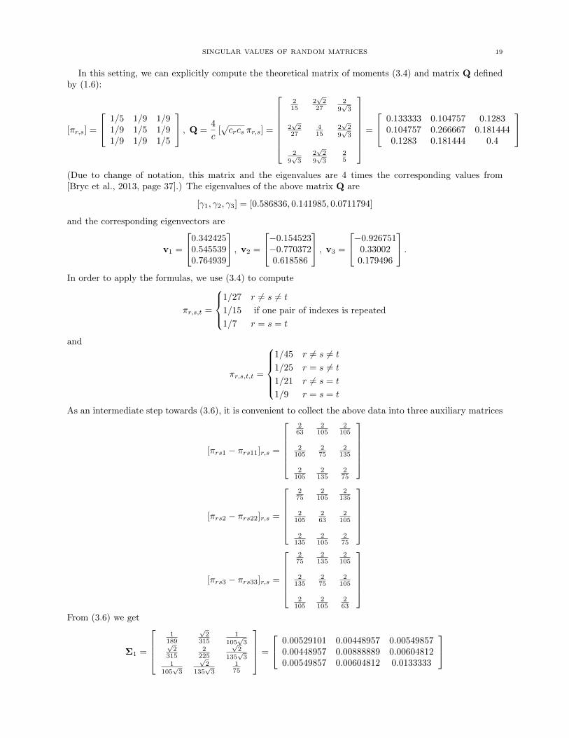
SINGULAR VALUES OF RANDOM MATRICES 19
In this setting, we can explicitly compute the theoretical matrix of moments (3.4) and matrix Q definedby (1.6):
[πr,s] =
1/5 1/9 1/91/9 1/5 1/91/9 1/9 1/5
, Q =4
c[√crcs πr,s] =
215
2√
227
29√
3
2√
227
415
2√
29√
3
29√
32√
29√
325
=
0.133333 0.104757 0.12830.104757 0.266667 0.1814440.1283 0.181444 0.4
(Due to change of notation, this matrix and the eigenvalues are 4 times the corresponding values from[Bryc et al., 2013, page 37].) The eigenvalues of the above matrix Q are
[γ1, γ2, γ3] = [0.586836, 0.141985, 0.0711794]
and the corresponding eigenvectors are
v1 =
0.3424250.5455390.764939
, v2 =
−0.154523−0.7703720.618586
, v3 =
−0.9267510.330020.179496
.In order to apply the formulas, we use (3.4) to compute
πr,s,t =
1/27 r 6= s 6= t
1/15 if one pair of indexes is repeated
1/7 r = s = t
and
πr,s,t,t =
1/45 r 6= s 6= t
1/25 r = s 6= t
1/21 r 6= s = t
1/9 r = s = t
As an intermediate step towards (3.6), it is convenient to collect the above data into three auxiliary matrices
[πrs1 − πrs11]r,s =
263
2105
2105
2105
275
2135
2105
2135
275
[πrs2 − πrs22]r,s =
275
2105
2135
2105
263
2105
2135
2105
275
[πrs3 − πrs33]r,s =
275
2135
2105
2135
275
2105
2105
2105
263
From (3.6) we get
Σ1 =
1
189
√2
3151
105√
3√2
3152
225
√2
135√
31
105√
3
√2
135√
3175
=
0.00529101 0.00448957 0.005498570.00448957 0.00888889 0.006048120.00549857 0.00604812 0.0133333

20 W LODEK BRYC AND JACK W. SILVERSTEIN
Σ2 =
1
189
√2
3151
105√
3√2
3152
225
√2
135√
31
105√
3
√2
135√
3175
=
0.00444444 0.00448957 0.004276670.00448957 0.010582 0.007776160.00427667 0.00777616 0.0133333
Σ3 =
1
225
√2
4051
105√
3√2
4052
225
√2
105√
31
105√
3
√2
105√
3163
=
0.00444444 0.00349189 0.005498570.00349189 0.00888889 0.007776160.00549857 0.00777616 0.015873
Using these expressions and (3.8) with c = M/N = 120/2500, we determine
[m1,m2,m3] = [0.183948√c+
0.174053√c
, 0.323598√c+
0.353849√c
, 0.47449√c+
0.49976√c
] = [0.834739, 1.68599, 2.38504].
We note that the shift is stronger for smaller singular values and is more pronounced for rectangular matriceswith small (or large) c.
Finally, we compute the covariance matrix
(3.13) [Eζrζs] =
0.306317 0.0293619 0.02256040.0293619 0.233577 −0.009416920.0225604 −0.00941692 0.235559
.The following figure illustrates that normal approximation works well.
410 411 412 413 414 415 4160
100
200
300
400
206 206.5 207 207.5 208 208.5 209 209.5 2100
100
200
300
400
143.5 144 144.5 145 145.5 146 146.5 147 147.50
100
200
300
400
Figure 2. Histograms of three largest singular values with normal curves centered at [√ρ1+
m1,√ρ2 + m2,
√ρ3 + m3] = [413.47, 208.02, 145.44] with variances 0.3063, 0.2336, 0.2356.
Based on 10,000 runs of simulations after a single randomization to choose vectors p1,p2,p3
with M = 120, N = 2500.
Based on simulations reported in Fig. 2, we conclude that normal approximation which uses the eigen-values of R0 provides a reasonable fit.

SINGULAR VALUES OF RANDOM MATRICES 21
Let us now turn to the question of asymptotic normality for the normalized squares of singular valuesΛr = λ2
r/(√M+√N)2. With M = 120, N = 2500 (correcting the misreported values) Ref. [Bryc et al., 2013]
reported the observed values (48.2, 11.5, 5.8) for Λ1,Λ2,Λ3 versus the “theoretical estimates” (47.4, 11.5, 5.7)
calculated as γrMN/(√M +
√N)2 in our notation. While the numerical differences are small, Proposition
3.4 restricts the accuracy of such estimates due to their dependence on the eigenvalues of R0 constructedfrom vectors of allelic probabilities pr. Figure 3 illustrates that different selections of such vectors from thesame joint allelic spectrum (3.4) may yield quite different ranges for Λ1,Λ2,Λ3. It is perhaps worth pointingout that the variance of normal approximation depends only on the allelic spectrum.
45.5 45.6 45.7 45.8 45.9 46 46.1 46.2 46.3 46.40
100
200
300
11.45 11.5 11.55 11.6 11.65 11.7 11.75 11.80
100
200
300
5.55 5.6 5.65 5.7 5.75 5.80
100
200
300
47.2 47.3 47.4 47.5 47.6 47.7 47.8 47.9 480
100
200
300
11.75 11.8 11.85 11.9 11.95 12 12.05 12.1 12.150
100
200
300
5.7 5.75 5.8 5.85 5.9 5.95 60
100
200
300
One random choice of pr Another random choice of pr
Figure 3. Two histograms of normalized squared singular values (Λ1,Λ2,Λ3), based on10000 simulations, and the theoretical normal curves from Proposition 3.4 drawn in red.This is M = 120 individuals with N = 2500 markers. Although the numerical differencesbetween the left-hand-side and the right-hand side are small, the histograms have practicallydisjoint supports.
References
[Billingsley, 2012] Billingsley, P. (2012). Probability and measure. Wiley Series in Probability and Statistics. John Wiley & Sons,
Inc., Hoboken, NJ. Anniversary edition [of MR1324786], With a foreword by Steve Lalley and a brief biography of Billingsleyby Steve Koppes.
[Bryc et al., 2013] Bryc, K., Bryc, W., and Silverstein, J. W. (2013). Separation of the largest eigenvalues in eigenanalysis of
genotype data from discrete subpopulations. Theoretical Population Biology, 89:34–43. arXiv:1301.451.[Furedi and Komlos, 1981] Furedi, Z. and Komlos, J. (1981). The eigenvalues of random symmetric matrices. Combinatorica,
1(3):233–241.
[Kimura, 1964] Kimura, M. (1964). Diffusion models in population genetics. Journal of Applied Probability, 1(2):177–232.[Lang, 1964] Lang, D. W. (1964). Isolated eigenvalue of a random matrix. Phys. Rev., 135:B1082–B1084.[Lata la, 2005] Lata la, R. (2005). Some estimates of norms of random matrices. Proceedings of the American Mathematical
Society, 133(5):1273–1282.[Patterson et al., 2006] Patterson, N., Price, A. L., and Reich, D. (2006). Population structure and eigenanalysis. PLoS Genet,
2(12):e190.
[Silverstein, 1994] Silverstein, J. W. (1994). The spectral radii and norms of large-dimensional non-central random matrices.Comm. Statist. Stochastic Models, 10(3):525–532.
[Stewart and Sun, 1990] Stewart, G. W. and Sun, J.-G. (1990). Matrix Perturbation Theory (Computer Science and ScientificComputing). Academic Press Boston.
[Tao, 2013] Tao, T. (2013). Outliers in the spectrum of iid matrices with bounded rank perturbations. Probability Theory and
Related Fields, pages 1–33.[Yin et al., 1988] Yin, Y., Bai, Z., and Krishnaiah, P. (1988). On the limit of the largest eigenvalue of the large dimensionalsample covariance matrix. Probability Theory and Related Fields, 78(4):509–521.

22 W LODEK BRYC AND JACK W. SILVERSTEIN
W lodek Bryc, Department of Mathematical Sciences, University of Cincinnati, PO Box 210025, Cincinnati, OH45221–0025, USA
E-mail address: [email protected]
Jack W. Silverstein, Department of Mathematics, Box 8205, North Carolina State University, Raleigh, NC
27695-8205, USA
E-mail address: [email protected]