Singular perturbations approach to localised surface-plasmon resonance: nearly

touching metal nano-spheres

Ory SchnitzerDepartment of Mathematics, Imperial College London,

South Kensington Campus, London SW7 2AZ, United Kingdom

Metallic nano-structures characterised by multiple geometric length scales support low-frequencysurface-plasmon modes, which enable strong light localisation and field enhancement. We suggestto study such configurations using singular perturbation methods, and demonstrate the efficacyof this approach by considering, in the quasi-static limit, a pair of nearly touching metallic nano-spheres subjected to an incident electromagnetic wave polarised with the electric field along the lineof sphere centres. Rather than attempting an exact analytical solution, we construct the pertinent(longitudinal) eigen-modes by matching relatively simple asymptotic expansions valid in overlappingspatial domains. We thereby arrive at an effective boundary eigenvalue problem in a half-spacerepresenting the metal region in the vicinity of the gap. Coupling with the gap field gives rise to amixed-type boundary condition with varying coefficients, whereas coupling with the particle-scalefield enters through an integral eigenvalue selection rule involving the electrostatic capacitance ofthe configuration. By solving the reduced problem we obtain accurate closed-form expressions forthe resonance values of the metal dielectric function. Furthermore, together with an energy-likeintegral relation, the latter eigen-solutions yield also closed-form approximations for the induced-dipole moment and gap-field enhancement under resonance. We demonstrate agreement between theasymptotic formulae and a semi-numerical computation. The analysis, underpinned by asymptoticscaling arguments, elucidates how metal polarisation together with geometrical confinement enablesa strong plasmon-frequency redshift and amplified near-field at resonance.

I. INTRODUCTION

Advances in micro-fabrication technology along withnew innovative ideas in nano-photonics and meta-materials have rekindled interest in the optics of smallmetal particles and structures [1–3]. Nano-metallic con-figurations exhibit unique optical characteristics, whichare largely associated with the excitation of localisedsurface-plasmon (LSP) modes: conjoint resonant oscilla-tions of electron-density and electromagnetic fields. LSPresonances are manifested in spectral peaks of the opticalcross-sections and in significant near-field enhancements.Such phenomena are attractive for sensing applications[4], plasmonic manipulation of light below the diffractionlimit [5], enhanced Raman scattering [6, 7], plasmonicrulers [8], lasers [9] and nanoantennas [10–12], second[13] and higher-order [14] harmonic generation, and pho-tovoltaics [15].LSP resonance is exemplified by light scattering from

a nano-metric metal sphere. In the quasi-static limit,the near-field, which appears to be driven by a uniformtime-harmonic field, is derived from an electric potentialgoverned by Laplace’s equation. The induced electric-dipole moment is readily found to be proportional to theClausius–Mossotti factor (ǫ − 1)/(ǫ + 2), where ǫ is thefrequency-dependent dielectric function of the metal par-ticle relative to its dielectric surrounding. The evident di-vergence at the Frohlich value ǫ = −2 is associated withan existence of a solution to the homogeneous quasi-staticproblem (in which the incident field is absent). At visibleand ultraviolet frequencies, a good approximation for the

Drude dielectric function is [16]

Re[ǫ] ≈ 1− ω2p/ω

2, Im[ǫ] ≈ ω2pγ/ω

3, (1)

where ω is the frequency of light, and ωp and γ arethe plasma and collision frequencies, respectively (rep-resentative values for noble metals: ~ωp ≈ 9 eV, ~γ ≈0.13 eV). Owing to the smallness of γ/ωp, a damped res-onance occurs when Re[ǫ] ≈ −2.LSP frequencies and the magnitude of resonant en-

hancement can be “designed” by shape and materialvariations [17–20]. Appreciable modification is achiev-able with “singular” configurations characterised by non-smoothness or multiple-scale geometries: sharp corners[21, 22], elongated particles [23–25], tips [26], nearlytouching [27–29], touching [30, 31], and embedded [32]particle pairs, “plasmonic molecules” [20], and particle-wall configurations [33]. A recurring feature encounteredin multiple-scale geometries is the existence of modes,that with increasing scale disparity, significantly redshiftto low frequencies and large −Re[ǫ] values.Singular configurations of the latter sort, which enable

a particularly strong near-field enhancement [34], havebeen extensively studied through numerical simulations[35–40], analytic solutions in separable coordinate sys-tems [21, 30, 41], and the powerful method of transforma-tion optics (TO) [42, 43]. In two dimensions TO furnishesexplicit solutions [22, 27, 28] that can be generalised toaddress effects of retardation [44] and non-locality [45].TO is less straightforward to apply in three dimensions,and typically furnishes an efficient computational scheme[46] rather than simple analytic expressions; neverthe-less, the method has been successfully applied in vari-ous scenarios, e.g. in the design of broadband plasmonic

2

structures [31] and in the study of van der Waals forces[29]. Yet another approach, motivated by general scalingarguments [47], is based on approximate reductions ofimplicit infinite-series solutions for nano-wire and nano-sphere dimers [48–50]; we delay a critical discussion of theaccuracy of the expressions in Refs. 48 and 50 to §VI.The above methodologies are “top-bottom” — neces-

sarily relying on “exact” analytical or numerical solu-tions, which then need to be reduced or evaluated in sin-gular geometric limits (e.g. small gaps for dimers, increas-ing aspect ratio for elongated particles). In this paper,we suggest an alternative “bottom-up” approach, whichis specifically suitable for analysing the extreme phys-ical characteristics of LSP resonance in multiple-scalemetallic nano-structures. The approach is built uponthe paradigm of singular perturbation methods, wherean asymptotic rather than an exact solution is sought bycarrying out an ab initio singular analysis. In particu-lar, applying asymptotic scaling arguments in conjunc-tion with the method of matched asymptotic expansions[51] allows exploiting the spatial non-uniformity of thesingular LSP modes towards systematically decompos-ing the problem governing these into several consider-ably simpler ones. The main outcomes are asymptoticexpressions for the resonance frequencies, along with aminimalistic description of the corresponding modes. Inthe context of excitation problems, when losses are lowan asymptotic approximation for the field enhancementmay be obtained with little additional effort.To demonstrate this approach, we shall focus in this

paper on the prototypical configuration of a pair of nearlytouching metal nano-spheres [35, 37, 39, 47, 48, 50, 52–57]. We limit ourselves to a quasi-static treatment ofthe near field, and focus on the axisymmetric and lon-gitudinal (bonding) modes that singularly redshift withvanishing gap width, and the excitation of these by along-wave electromagnetic plane wave polarised with theelectric field along the line of centres. The paper proceedsas follows. In §II we formulate the problem and note use-ful generalities. In §III we consider the plasmonic eigen-value problem and obtain closed-form expressions for thedielectric-function resonance values. In §IV we employthe eigenvalues and eigen-potentials found in §III to ob-tain formulae for the induced dipole moment and fieldenhancement in the gap under resonance conditions. In§V we present a validation of our results against a semi-numerical solution of the quasi-static problem. Lastly,in §VI we recapitulate our results, compare with relatedworks, and discuss recent developments along with futuredirections.

II. PRELIMINARIES

A. Problem formulation

Consider an identical pair of metal spheres surroundedby a dielectric medium. The spheres are characterised

a

metal nano-spheres

dielectric

mediumquasi-static incident

electric field

E Re[

e−iωt

]

2ha

ı

FIG. 1. Schematics of the quasi-static excitation problem.

by their radius a, and their frequency-dependent dielec-tric function relative to the background material, ǫ0ǫ, ǫ0being the vacuum permittivity. The minimum separa-tion between the spheres is denoted by 2ha. The pair issubjected to an incident time-harmonic electromagneticplane wave of frequency ω, polarised such that the electricfield is in a direction ı parallel to the line of sphere cen-tres, see Fig. 1. We shall focus on the quasi-static limitof sufficiently small particles, a≪ c/(ω

√

|ǫ|), c being thespeed of light in the surrounding dielectric [16, 58]. Inthis description, the pair experiences the incident waveas a uniform time harmonic field ıERe[e−iωt], where Eis a real constant magnitude, and the electric near-fieldis approximately curl-free, derived from a time-harmonicpotential aERe[ϕe−iωt].Henceforth, we normalise all lengths by a. In partic-

ular, we denote by x the dimensionless position vectorrelative to the centre of the gap. It is convenient to em-ploy a cylindrical coordinate system (r, z, φ), with originat x = 0 and a z-axis directed along ı (see Fig. 2). Theproblem at hand is to find a continuous potential ϕ thatsatisfies

∇ · (E∇ϕ) = 0, (2)

where E is unity in the dielectric medium and ǫ in themetal spheres, together with the far-field condition

ϕ ∼ −z + o(1) as |x| → ∞. (3)

The additive freedom of ϕ is removed in (3) by choosingthe disturbance from the incident field to attenuate atlarge distances.

B. General properties

The following generalities can be inferred from (2)–(3), see also Refs. [3, 36, 59–61]. First, the potentialis axisymmetric about the ı axis, i.e. ∂ϕ/∂φ = 0. Inaddition, the potential is antisymmetric about the planez = 0. It is therefore possible to consider only the half-space z > 0, with

ϕ = 0 at z = 0. (4)

3

We next note that each of the spheres is overall chargefree. That is,

∮

∂ϕ

∂ndA = 0, (5)

where the integration is over an arbitrary closed surfaceentirely within the dielectric medium, which encloses oneor both spheres. Thus ϕ lacks a monopole term in its far-field expansion (3), which can therefore be extended to

ϕ ∼ −z + µz

|x|3 as |x| → ∞. (6)

The complex-valued constant µ is the induced dipole mo-ment of the pair, normalised by 4πa3ǫ0ǫdE (ǫd being therelative dielectric constant of the surrounding medium).Green identities applied to ϕ and its complex conjugate

ϕ∗, in conjunction with (2) and (6), can be shown to give

4πIm[µ] = Im[ǫ]

∫

metal

∇ϕ · ∇ϕ∗ dV, (7)

where the integration is over the volume of the twospheres. Eq. (7) is a work-dissipation relation: The workdone by the incident field on the effective induced dipoleof the dimer is lost to Ohmic dissipation in the metal.This relation serves to remind us that we are in the quasi-static limit, where radiation losses are negligible. Wenote that 4πIm[µ] gives the quasi-static approximationfor the absorption cross-section normalised by ωa3/c [2].Excitation problems of the above sort are ill posed for

a set of discrete, real and negative, ǫ values, for which thehomogeneous variant of the problem obtained by omit-ting the incident field in (3) possesses non-trivial solu-tions. Since in practice Im[ǫ] 6= 0, such solutions areoften termed “virtual” LSP modes. Consider now aneigen-potential ϕr corresponding to one such eigenvalueǫr. At large distances,

ϕr ∼ µrz

|x|3 as |x| → ∞, (8)

where µr is arbitrary. We note that the integral relation(7) does not apply to ϕr, since condition (3) is used toderive it. Say, however, that ϕ is the solution to theactual quasi-static problem, with ǫ = ǫr +∆ǫ. Applyingthe Green identities to the pair of potentials (ϕ, ϕr), onecan easily show that

4πµr = −∆ǫ

∫

metal

∇ϕr · ∇ϕdV. (9)

Whereas (7) bears a clear physical significant, we shallfind in §IV that (9) is more useful for deriving quantita-tive estimates for the resonant field enhancement.

C. Near-contact limit

Henceforth we consider the near-contact limit whereh→ 0. Specifically, our goal will be to derive closed-form

anti-symmetry

plane

incident

field

metal dielectric

function relative

to surrounding

1

ϕ = 0

h

ϕ ∼ −z + µz

|x|3φ

z

r

induced

dipole

moment

field enhanchment

in gap

ǫ

ı

G = −

(

∂ϕ

∂z

)

x=0

FIG. 2. Schematics of the dimensionless excitation problem.

asymptotic formulae for the eigenvalues ǫ(n), and the val-ues at resonance conditions (i.e. when Re[ǫ] = ǫ(n)) of theinduced-dipole moment µ and the field enhancement inthe gap, G = − (∂ϕ/∂z)

x=0.

III. LSP MODES

In this section we consider the boundary eigenvalueproblem obtained by replacing the far field (3) with thehomogeneous condition ϕ → 0 as |x| → ∞. It is clearthat the only relevant modes are those that are bothlongitudinal, i.e. anti-symmetric about the plane z = 0,and axisymmetric.

A. Scaling arguments

How do the eigenvalues ǫ scale with h? In the vicinityof the gap the spherical boundaries can be approximatedby two oppositely facing paraboloids. The separationtherefore remains O(h) for O(h1/2) radial distances. Weshall refer to the subdomain of the dielectric mediumwhere z = O(h) and r = O(h1/2) as the gap domain,and assume without loss of generality that the eigen-potential ϕ corresponding to ǫ is O(1) there; since ϕ isantisymmetric about the z plane, the transverse gap fieldmust be O(1/h). Consider now the particle-scale dielec-tric “outer” domain, away from the gap, where ϕ variesover distances |x| = O(1) and is at most O(1). It followsfrom (4) that ϕ = O(h) when z = O(h) and r = O(1).This implies that the gap potential must vary in the ra-dial direction over O

(

h1/2)

distances. Consider next themetal sphere in z > 0, in the vicinity of the gap boundary.Continuity of potential implies that ϕ is O(1) there, andvaries rapidly over O

(

h1/2)

distances along the bound-ary. On the latter length scale, the metallic volume ap-pears transversely semi-infinite. Thus, the symmetry of

4

Laplace’s equation implies comparably rapid transversevariations. We shall refer to the metal subdomain wherer, z = O(h1/2) as the pole domain.The scaling of ǫ now follows by considering the continu-

ity of electric displacement across the gap-pole interface:The product of ǫ and the O(h−1/2) transverse field in themetal pole must be on the order of the O(1/h) transversefield in the gap. We accordingly find

ǫ ∼ −h−1/2λ(h) +O(1), 0 < λ = O(1), (10)

where, as we shall see, the pre-factor λ itself dependsweakly upon h, being a function of ln(1/h). This moresubtle feature can also be anticipated from scaling argu-ments, as we now discuss.The largeness of |ǫ| suggests that, on the particle-

scale, the spheres are approximately equipotential. Thus,the particle-scale potential distribution in the dielectricmedium is approximately that about a pair of nearlytouching spheres held at uniform potentials, say ±V .But the latter distribution implies a net charge on eachsphere, in contradiction with (5). This means that thedeviation in the vicinity of the gap of ϕ from the particle-scale distribution must be consistent with a localised ac-cumulation of charge such that the overall charge of eachsphere is zero. In fact, the contributions to the integral in(5) from the gap and outer dielectric domains are readilyseen to be comparable: The former is given by the inte-gral of an O(1/h) transverse field over an O(h) surfacearea, while the latter is obviously O(1). This implies aconnection between the solution in the gap and pole “in-ner” domains, and the capacitance of a pair of perfectlyconducting spheres held at fixed potentials ±V , which isknown from electrostatic theory to depend logarithmi-cally upon h as h→ 0 [62].

B. Gap and pole domains

We begin constructing the eigen-potentials by consid-ering the gap domain. To this end, we introduce thestretched coordinates

R = r/h1/2, Z = z/h. (11)

The gap domain is where R,Z ∼ O(1), with R > 0 andZ bounded by the spherical surfaces (see Fig. 3)

Z ∼ ±H(R) +O(h), where H(R) = 1 +1

2R2. (12)

As in §III A, we assume without loss of generality thatϕ = O(1) in the gap domain. We accordingly pose theasymptotic expansion

ϕ ∼ Φ(R,Z) +O(

h1/2)

. (13)

Substituting (13) into Laplace’s equation, written interms of R and Z, yields at leading order

∂2Φ

∂Z2= 0. (14)

ϕ ∼ ϕ

outer

domain

ξ ∼ 1 +O(h)

η = 0

η → ∞

ξ = const

η = const

tangent-sphere

coordinates

(ξ, η, φ)

gap domain

pole

domain

ϕ ∼ Φ

Z = z/h1/2

R = r/h1/2

Z ∼ H(R) +O(h)

Z ∼ O

(

h1/2

)

R = r/h1/2

Z = z/h

ϕ ∼ Φ

ψ = Φ− V

ϕ ∼ V

z

r

ξ = 0

FIG. 3. The resonant modes are constructed in §III by match-ing simple asymptotic expansions describing the gap, pole,and particle-scale “outer” domains.

Integration of (14) in conjunction with (4) gives

Φ = A(R)Z, (15)

where the function A(R) remains to be determined.Consider next the pole domain of the metal sphere

in z > 0, described by the alternative pair of stretchedcoordinates

R = r/h, Z = z/h1/2. (16)

The pole domain is where R, Z ∼ O(1), with R > 0 and Zbounded from below by the sphere surface Z ∼ O(h1/2);under the rescaling (16), the pole domain is to leadingorder a semi-infinite half space. We expand the pole-domain potential as

ϕ ∼ Φ(R, Z) +O(

h1/2)

, (17)

where Φ is governed by Laplace’s equation,

1

R

∂

∂R

(

R∂Φ

∂R

)

+∂2Φ

∂Z2= 0. (18)

Expanding the eigenvalue ǫ according to (10), requir-ing leading-order continuity of potential and electric dis-placement yields

Φ = Φ,∂Φ

∂Z+λ

∂Φ

∂Z= 0 at Z = H(R), Z = 0. (19)

5

Eqs. (19) may be combined to yield the mixed-typeboundary condition

Φ + λH∂Φ

∂Z= 0 at Z = 0, (20)

which involves Φ alone. We also find the relation

A(R) =1

H

(

Φ)

Z=0, (21)

which provides the gap potential once the pole poten-tial has been determined. As discussed in §III A, theparticle-scale metal domain is equipotential to leading or-der. Asymptotic matching thus furnishes the “far-field”condition

Φ → V as R2 + Z2 → ∞, (22)

where V is the above-mentioned uniform potential of thesphere in z > 0. For later reference, we note that (21)and (22) imply Φ ∼ 2VZ/R2 as R→ ∞.The pole potential Φ is governed by Laplace’s equation

(18) in the half space Z > 0, the boundary condition (20),and the far-field condition (22). We shall see in §III Fthat this boundary-value problem possesses non-trivialsolutions for essentially arbitrary λ > 0 and V , excludinga discrete set of λ values for which a solution exists onlyif V is set to zero. It is tempting to guess that the latterset furnishes the requisite eigenvalues; we shall see in§III E however that these only give a leading term in anexpansion of λ in inverse powers of ln(1/h). Avoidingsuch gross logarithmic errors, the eigenvalues cannot besolely determined from local considerations, as alreadyanticipated in §III A. We accordingly divert at this stageto consider the particle-scale dielectric domain.

C. Outer domains and global constraint

In the outer limit, h → 0 with x = O(1), the spheresappear to be in contact to leading order. It is thereforeconvenient to introduce the tangent-sphere coordinatesdefined through [63]

z =2ξ

ξ2 + η2, r =

2η

ξ2 + η2. (23)

The plane z = 0 is mapped to ξ = 0, the upper-half-spacesphere to ξ ∼ 1 + O(h), and the origin to η → ∞ (seeFig. 3). We expand the potential in the outer dielectricdomain as

ϕ ∼ ϕ+O(h1/2), (24)

and in the outer metal domain as

ϕ ∼ ±V +O(h1/2), (25)

the ± sign corresponding to the sphere in z ≷ 0, respec-tively.

For ϕ we require a solution to Laplace’s equation thatattenuates at large distances and satisfies ϕ = V at ξ = 1and ϕ = 0 at ξ = 0. In addition, the solution mustasymptotically match the gap and pole potentials. Stan-dard Hankel-Transform methods yield the requisite po-tential as [62]

ϕ ∼ V(ξ2 + η2)1/2∫ ∞

0

e−s sinh(sξ)

sinh sJ0(sη) ds, (26)

where J0 is the zeroth-order Bessel function of the firstkind. It may be readily shown that ϕ ∼ 2Vz/r2 asη → ∞, whereby (26) matches with the gap and poledomains. Asymptotic evaluation of (26) for small ξ andη, together with (23), yields the asymptotic behaviour of(26) at large distances [cf. (8)],

ϕ ∼ π2V3

z

|x|3 as |x| → ∞. (27)

The leading-order matching of (26) with the solutionin the gap and pole regions has been achieved, appar-ently without introducing any additional constraint onthe problem governing Φ. Instead of continuing theasymptotic analysis to the next order in search of theawaited eigenvalue selection rule, it proves simpler tofollow the discussion in §III A and consider the chargeconstraint (5) applied to the sphere in z > 0. In accor-dance with the discussion there, an attempt to calculatethe contributions to the integral in (5) from the gap andouter region separately results in diverging integrals —this is typical in cases where contributions from overlap-ping asymptotic domains are comparable [51]. Followingthe analysis in Ref. [62], we write (5) as

∫ R0

0

A(R)RdR +

∫ η0

0

∂ϕ

∂ξ

∣

∣

∣

∣

ξ=1

2η

1 + η2dη = O

(

h1/2)

,

(28)where η0, R0 ≫ 1 are connected through h1/2R0 = 2/η0+O(1/η30). The first integral in (28), which represents theexcess contribution from the gap region, can be writtenas

∼∫ ∞

0

[

A(R)− VH(R)

]

RdR+ V lnH(R0). (29)

The second integral in (28), which represents the contri-bution of the outer domain, can be worked out to be

∼ V[

2γe + ln(1 + η20)]

, (30)

where γe ≈ 0.5772 is the Euler–Gamma constant. Notingthat lnH(R0) ∼ ln(2/h) − ln η20 , and invoking (21), thesingular parts of the two contributions cancel out, andwe find the anticipated “global” constraint:

V = − 1

ln(2/h) + 2γe

∫ ∞

0

Φ(R, 0)− VH(R)

RdR. (31)

6

D. Reduced eigenvalue problem

Together with (31), the problem governing the polepotential Φ constitutes a reduced boundary-eigenvalueproblem. It is convenient to recapitulate this problem interms of the disturbance potential, ψ(R, Z) = Φ−V . Wehave Laplace’s equation

1

R

∂

∂R

(

R∂ψ

∂R

)

+∂2ψ

∂Z2= 0 (32)

in the upper half-space Z > 0, the integro-differentialvarying-coefficient boundary condition

ψ + λH(R)∂ψ

∂Z=

1

ln(2/h) + 2γe

∫ ∞

0

ψ(R, 0)

H(R)RdR (33)

at Z = 0 [we will sometimes write −V for the right-hand-side, see (31)], and the far-field condition

ψ → 0 as R2 + Z2 → ∞. (34)

The logarithmic dependence of the eigenvalues λ andtheir corresponding eigen-potentials ψ upon h is evidentfrom (33). We also see that a rough leading-order solu-tion, entailing an O(ln−1 1

h ) relative error, may be ob-tained by neglecting the right hand side of (33). Inthe following subsections we proceed in two paths: (i)in §III E we calculate succesive terms in inverse logarith-mic powers; (ii) in §III F we tackle the reduced eigenvalueproblem as a whole, thereby finding an “algebraically ac-curate” approximation for the resonance ǫ values.

E. Two terms in a logarithmic expansion

We here expand the potentials ψ and the eigenvaluesλ as

ψ ∼ ψ0 +1

ln 1h

ψ1 + · · · , λ ∼ λ0 +1

ln 1h

λ1 + · · · (35)

At leading order, the boundary condition (33) reads

ψ0 + λ0H(R)∂ψ0

∂Z= 0 at Z = 0. (36)

We look for a solution in the form

ψ0(s, Z) = H[

ψ0(R, Z)]

, (37)

where

H[f(R)](s) =

∫ ∞

0

f(R)J0(sR)RdR (38)

is the zeroth-order Hankel transform [64]. Applying theHankel transform to Laplace’s equation (32), a solutionthat satisfies (34) is

ψ0 =1

sY0(s)e

−sZ , (39)

where Y0(s) depends on the conditions at Z = 0. Trans-forming the boundary condition (36), we find the s-spacedifferential equation

1

s

d

ds

(

sdY0ds

)

+ 2

(

1

λ0s− 1

)

Y0 = 0. (40)

The first term in (40) is obtained through integration byparts twice, which is only applicable if [64]

Y0 ≪ 1

s2and

dY0ds

≪ 1

sas s→ 0. (41)

In addition, Y0(s) must decay sufficiently fast to allowconvergence of (37). Defining

Y0(s) = e−√2sT0(p), p = 2

√2s, (42)

substitution shows that T (p) satisfies Laguerre’s equation

pd2T0dp2

+ (1 − p)dT0dp

+1

2

(√2

λ0− 1

)

T0 = 0. (43)

Non-singular solutions of the latter, which are consistentwith (41) and the required attenuation rate of Y0(s), ex-ist only when the factor multiplying T in (43) is a non-negative integer. In those cases the solutions are propor-tional to the Laguerre polynomials. Hence, the leading-order eigenvalues are

λ(n)0 =

√2

2n+ 1, n = 0, 1, 2, . . . (44)

The corresponding transformed solutions are

Y(n)0 (s) = K(n)e−

√2sLn(2

√2s), (45)

where K(n) is an arbitrary constant, and Ln is the Legen-dre polynomial of order n. It is straightforward to invert

(37) to get the eigen-potentials ψ(n)0 . For example, not-

ing that L0(p) = 1 and L1(p) = 1−p, the first two modesare

ψ(0)0 =

K(0)

[

R2 + (Z +√2)2]1/2

(46)

and

ψ(1)0 = ψ

(0)0 − 2

√2K(1)(Z +

√2)

[

R2 + (Z +√2)2]3/2

. (47)

Proceeding to the next logarithmic order, we see that

the problem governing ψ(n)1 is similar to the one govern-

ing ψ(n)0 , only that the homogeneous boundary condition

(36) is replaced by an inhomogeneous one. Dropping the(n) superscript for the moment, the latter condition fol-lows from (33) as

ψ1 + λ0H(R)∂ψ1

∂Z=λ1λ0ψ0 +

∫ ∞

0

ψ0R

H(R)dR. (48)

7

From the preceding analysis it is clear that, when λ0is given by (44), the problem governing ψ1 possesses anontrivial homogeneous solution. Hence, the Fredholmalternative suggests a solvability condition on the forcingterms in (48). Indeed, by subtracting (48) multipliedby Rψ0/H from (36) multiplied by Rψ1/H , followed byintegration with respect to R and use of Green’s secondidentity, we find

λ1 = −λ0(∫ ∞

0

ψ0R

H(R)dR

)2/

∫ ∞

0

ψ20R

H(R)dR. (49)

The integrals in (49) can be readily evaluated by useof Parseval’s identity and the inversion-symmetry of theHankel transform, together with the orthonormality ofthe Laguerre polynomials, see (A.1). One finds the sim-

ple result λ1 = −2√2 (λ0)

2, whereby reinstating the (n)

superscript gives the two-term logarithmic expansion

λ(n) ∼√2

2n+ 1

(

1− 4

2n+ 1

1

ln(1/h)+ · · ·

)

. (50)

F. Algebraically accurate result

It is clear that the logarithmic error in (50) limits theusefulness of that result to exceedingly small h. To im-prove on this, we now return to the reduced problem of§III D and attempt a complete solution for the λ eigenval-ues, treating logarithmic terms in par with O(1) terms.This is equivalent to calculating all of the terms in expan-sion (35). We begin by writing the solution as [cf. (37),(38) and (39)]

ψ = H−1[ψ], where ψ =1

sY (s)e−sZ . (51)

Applying the Hankel transform to (33), we find

1

s

d

ds

(

sdY

ds

)

+ 2

(

1

λs− 1

)

Y = −4Vλ

δ(s)

s, (52)

where δ(s) is the Dirac delta function. Eq. (52) is tobe interpreted in the sense of distributions [65], which iseasier to do when identifying the Hankel transform as atwo-dimensional Fourier transform of a radially symmet-ric function, s being the radial distance in Fourier-space.Crucially, conditions (41) are now inapplicable; rather,balancing singularities at the origin yields the condition

Y (s) ∼ −2Vλ

ln s as s→ 0. (53)

Following (42), we set Y (s) = e−√2sT (p), where p =

2√2s. This gives [cf. (43)]

pd2T

dp2+ (1 − p)

dT

dp+ nT = 0, p > 0, (54)

where n is defined through

λ =

√2

2n+ 1. (55)

We arrive at an eigenvalue problem consisting of (54),the “boundary” condition

T (p) ∼ −2Vλ

ln p as p→ 0, (56)

and the condition that T does not grow too fast asp→ ∞. The solutions found in §III E, which correspondto non-negative integer n and V = 0, are inconsistentwith condition (56). Hence, in the present scheme, wherelogarithmic errors are not tolerated, V 6= 0. In the lat-ter case, excluding non-negative integer n, solutions of(54) which are logarithmically singular as p → 0 andhave acceptable behaviour at large p are proportionalto U(−n, 1, p), where U is the confluent hypergeometricfunction of the second kind [66]. Noting that

U(−n, 1, p) ∼ − 1

Γ(−n) [ln p+Ψ(−n) + 2γe]+o(1) (57)

as p→ 0, where Γ(x) is the Gamma function and Ψ(x) =Γ′(x)/Γ(x) is the Digamma function, condition (56) issatisfied by

T (p) =2Vλ

Γ(−n)U(−n, 1, p). (58)

It remains to satisfy the global condition, that is, torelate V to the right hand side of (33) [cf. (31)]. It isconvenient to first rewrite that condition as

ln2

h+ 2γe =

∫ ∞

0

(

λ∂

∂Z(ψ/V) + 1

H

)

RdR. (59)

The integral on the right can be evaluated by using Parse-val’s identity. Noting that the Hankel transform of 1/H

is 2K0(s√2), K0 being the modified Bessel function of

the second kind, that integral is

2

∫ ∞

0

[

−λ

V Y (s) + 2K0

(

s√2)

]

δ(s) ds. (60)

Given (57), and since K0(x) ∼ − ln(x/2) − γe as x →0, the apparent logarithmic singularity of the brack-eted terms cancels, whereby the sifting property of theDirac delta function can be effected to show that (60)= 2 ln 4 + 2Ψ(−n) + 2γe. Substitution of this result into(59) furnishes a transcendental equation for n:

2Ψ(−n) = ln1

8h. (61)

Since Ψ(x) diverges at non-positive integer x, it is easy tosee that (61) has multiple non-integer solutions n which(very slowly) approach n = 0, 1, 2, as h→ 0 [67].

8

R0 0.5 1 1.5 2 2.5

A(R

)=

∂Φ/∂Z

-10-505

1015

1

2

n = 0

FIG. 4. The radial distribution of the dimensionless trans-verse field in the gap for the longitudinal modes n = 0, 1 and2, for h = 0.001 and V = 1.

Recapitulating, definition (55) furnishes the eigenval-ues as

λ(n) =

√2

2n(h) + 1, (62)

where n is the solution of (61) which approaches n =0, 1, 2, . . . as h→ 0. We reiterate that (62) is algebraicallyaccurate, viz., together with (10) it provides the reso-nance values of the relative dielectric function up to arelative error which scales with some power of h. In par-ticular, (62) is far more accurate then (50). We note thatit is straightforward to recover (50) by expanding Ψ in(61) about its poles. Higher order logarithmic terms can

be derived in a similar manner. Inverting ψ provides thedistribution of the eigenpotentials in the pole to algebraicorder [cf. (46) and (47)]. The dominantly transverse fieldin the gap, which is a function ofR alone, is then obtained(up to a minus sign) as ∂Φ/∂Z = A(R) = ψ(R, 0)/H(R).The radial gap-field distributions of the first three modesare plotted in Fig. (4).

IV. INDUCED-DIPOLE MOMENT AND FIELD

ENHANCEMENT

A. Resonance conditions

We now return to the excitation problem formulatedin §II, where the far-field condition (3) applies, and ǫ isa complex-valued function of frequency. Whereas a neg-ative real ǫ is unphysical, the reduced Drude model (1)implies that −Re[ǫ] ≫ Im[ǫ] as long as ω ≫ γ. Reso-nance frequencies are safe within this range: even for anextremely narrow gap, say h = 10−4, Eqs. (1) and (10)suggest ω ≈ 0.1ωp — still quite larger than γ for silverand gold. Thus, towards studying the damped near-fieldresonance of the system, it is useful to consider a reso-nance scenario

ǫ ∼ ǫ(n) + iǫi, ǫi ≪ h−1/2. (63)

Here, for a given n = 0, 1, 2, . . ., ǫ(n) is a resonance value∼ −λ(n)(h)h−1/2 + O(1), where λ(n) = O(1) is given by

(62), and iǫi is the imaginary deviation from the reso-nance values.Given (63), it turns out that an asymptotic descrip-

tion of the field distribution — and in particular, closed-form approximations for the induced-dipole moment µand field enhancement in the gap G — can be obtainedbased on the LSP modes calculated in §III. The crucialobservation is that the nth LSP mode is “excited” un-der (63), viz., the leading-order potential is of the formcalculated in §III, but with an asymptotically large mul-tiplicative factor. Note that if the potential was not ≫ 1,(63) would imply a contradictory leading-order problemwhich, on the one hand, possesses a non-trivial homoge-neous solution, and on the other, is forced at large dis-tances by the incident field. Thus, the integral relation(9) can be written, asymptotically, as

4πµ ∼ −iǫi∫

metal

∇ϕ · ∇ϕdV. (64)

We can now substitute our solutions from §III (allowingfor a large pre-factor) into (64), and solve for the am-plification factor (say, in terms of µ). We note that, incontrast to (64), the work-dissipation relation (7) is am-biguous with respect to phase and hence cannot be em-ployed towards making quantitative assessments withoutfurther information. We once more precede a detailedanalysis with scaling arguments.

B. Scaling arguments

Let ϕg denote the order-of-magnitude of the poten-tial in the gap region. The asymptotic structure of thepotential then follows from the description provided in§III. In particular, the transverse field in the gap isG = O(ϕg/h), the potential in the pole region is O(ϕg),and on the particle scale the sphere is approximatelyequipotential, with V = O(ϕg/ ln(1/h)), see (31). Notethat (27) implies µ = O(V). Consider now the integralon the right hand side of (64) [the work-dissipation re-lation (7) can also be employed]. The dominant contri-bution arises from the pole domains, where the potentialvaries rapidly. Indeed, the volume of the pole domains isO(h3/2) and the integrand there is O(ϕ2

g/h), leading to an

O(ϕ2gh

1/2) estimate. The contribution from the approx-

imately equipotential O(1) volume is O(ϕ2gh) at most.

We thus find from (64) that ϕg = O(h−1/2/(ǫi ln(1/h))),from which estimates for µ and G readily follow as

µ ∼ O

(

1

ǫi h1/2 ln2 1

h

)

, G ∼ O

(

1

ǫi h3/2 ln1h

)

. (65)

9

C. Asymptotic formulae

To go beyond scaling arguments, we use Green’s firstidentity together with (5) to rewrite (64) as

µ ∼ −iǫih1/2∫ ∞

0

(

ψ∂ψ

∂Z

)

Z=0

RdR, (66)

where ψ denotes the deviation of the potential in the(z > 0) pole domain from V , see §III. Applying Parse-val’s theorem to the right-hand-side of (64), it becomes[cf. (51)]

∼ iǫih1/2

∫ ∞

0

Y 2(s) ds. (67)

Upon substitution of Y (see below), and noting that µ ∼π2V/3 [cf. (27)], (66) can be solved for V , and hence µ.The field enhancement we can then be obtained from

G ∼ − 1

h

∂Φ

∂Z, (68)

where Φ is the gap potential [cf. (13)], and the derivativeis evaluated at R,Z = 0. Using (19), G can also bewritten as

∼ λ

h

∂ψ

∂Z, (69)

where the derivative is evaluated at R = 0, Z = 0, or interms of Y (s),

∼ −λh

∫ ∞

0

sY (s) ds. (70)

The calculation can be performed at two levels, de-pending on whether the logarithmically or algebraicallyaccurate expressions for Y and λ are employed in theabove formulae. We start with the former case, substi-tuting Y0(s) for Y (see (45)) and λ0 for λ (see (44)).Noting (31), the arbitrary constant K in Y0 is to within alogarithmic relative error K ∼ V ln 1

h/λ0. Together withthe integrals (A.1) and (A.2), we find the explicit closed-form expressions

µ ∼ 4√2π4

9(2n+ 1)2iǫi h1/2 ln2(1/h)

(71)

and

G ∼ (−1)n+12√2π2

3(2n+ 1)iǫi h3/2 ln(1/h). (72)

Expressions (71) and (72) have the advantage of beingsimple, but since they entail an O(1/ ln(1/h)) error, theyare hardly accurate, as we shall later demonstrate. Wenote the agreement with the scaling results (65), and thatthe excited resonant mode is imaginary, i.e. out of phasewith the incident field.

To obtain algebraically accurate formulae, we substi-tute (58) for Y and (62) for λ. Making use of the in-tegrals (A.3) and (A.4), the solution scheme describedabove yields

µ ∼√2π4

9iǫih1/2(2n+ 1)2Ψ′(−n) (73)

and

G ∼ −√2π2

12iǫih3/2Γ(−n) 2F1(2, 2, 2− n, 1/2)

(2n+ 1)2Ψ′(−n)Γ(2− n), (74)

where Ψ′(x) is the TriGamma function, the derivativeof the DiGamma function, 2F1 is the hypergeometricfunction, and n is as before the solution of (61) thatapproaches n = 0, 1, 2, . . . as h → 0. We note that(71) and (72) can be derived as leading approximationsof (73) and (74), respectively, by noting that n − n ∼2/ ln(1/h) as h → 0, and that Ψ′(−n) ∼ −(n − n)−2,

2F1(2, 2, 2− n, 1/2)/Γ(2− n) ∼ 4n!(2n+1) and Γ(−n) ∼(−1)n+1/[n!(n− n)] as n→ n.

V. COMPARISON WITH SEMI-NUMERICAL

SOLUTION

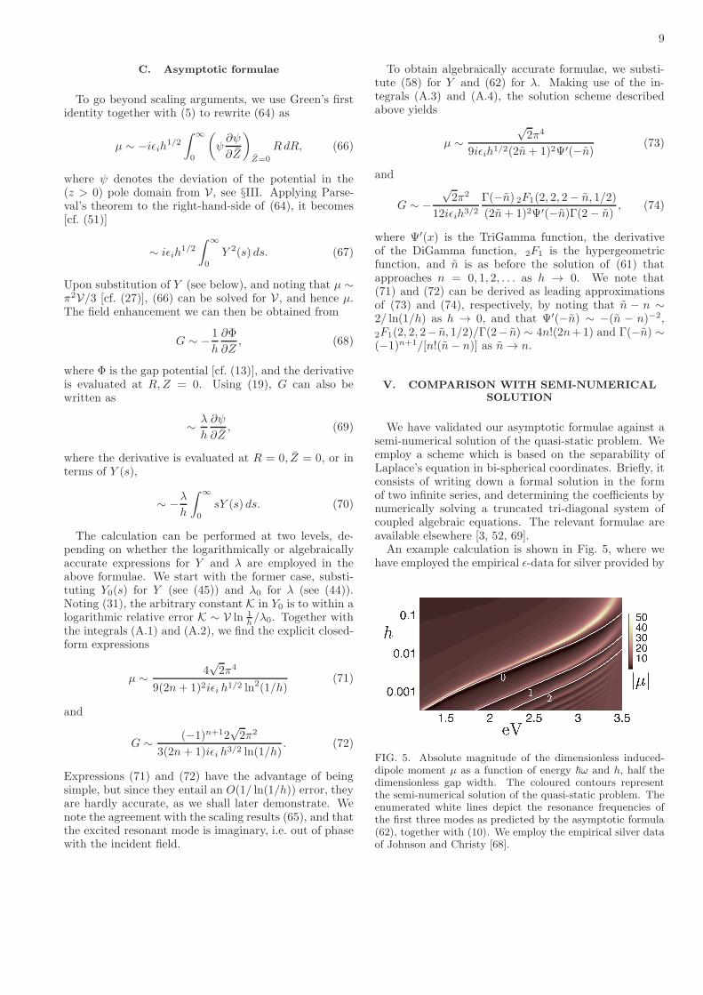
We have validated our asymptotic formulae against asemi-numerical solution of the quasi-static problem. Weemploy a scheme which is based on the separability ofLaplace’s equation in bi-spherical coordinates. Briefly, itconsists of writing down a formal solution in the formof two infinite series, and determining the coefficients bynumerically solving a truncated tri-diagonal system ofcoupled algebraic equations. The relevant formulae areavailable elsewhere [3, 52, 69].An example calculation is shown in Fig. 5, where we

have employed the empirical ǫ-data for silver provided by

FIG. 5. Absolute magnitude of the dimensionless induced-dipole moment µ as a function of energy ~ω and h, half thedimensionless gap width. The coloured contours representthe semi-numerical solution of the quasi-static problem. Theenumerated white lines depict the resonance frequencies ofthe first three modes as predicted by the asymptotic formula(62), together with (10). We employ the empirical silver dataof Johnson and Christy [68].

10

h10-3 10-2 10-1 100 10

−ǫ

100

101

102

2

algebraically accurateasymptotics

two-termlogarithmicexpansion

√

2/h

FIG. 6. Zeroth-mode ǫ-eigenvalue as a function of h, half thedimensionless gap width. Results of a semi-numerical solution(symbols) are compared with the first term and two terms ofthe logarithmic expansion (50), and the algebraically accurateapproximation (62), cf. (10). Note also the approach of ǫ to−2 at large h.

Johnson and Cristy [68]. Fig. 5 shows the absolute mag-nitude of the induced-dipole moment µ as a function ofthe dimensional energy ~ω in eV units, for a range of h.We observe magnitude peaks which, as expected, redshiftas h→ 0. The white lines in Fig. 5 depict the first threeresonance frequencies as predicted from the asymptoticformula (62) in conjunction with the data of Johnson andCristy. For small h the latter lines successfully trace theamplitude peaks. Detailed results for the zeroth-mode ǫ-eigenvalues are shown in Fig. 6. It depicts as a function ofh the numerically obtained eigenvalues (symbols) alongwith the predictions of (62) and the two-term expansion(50). The asymptoticness of (62) as h → 0 is evident,with good agreement for h . 0.02 (i.e. radius-to-gap ra-tio of ≈ 25). As expected, the logarithmically accurateapproximations are quite poor. Note the approach atlarge h of ǫ to −2, the Frohlich value of isolated spheres.Consider next the values of µ andG. Focusing again on

the zeroth-mode, we have recorded for a range of h thenumerical values attained by µ and G at their zeroth-mode peaks. The absolute magnitude of these values(which are predominantly imaginary at resonance) aredepicted by the symbols in Fig. 7. The latter numeri-cal values are compared with the logarithmically accu-rate asymptotic approximations (71) and (72) — dashedlines, and the algebraically accurate approximations (73)and (74) — thick lines. Again we see that the latterapproximations are rather good, whereas the former arepoor for realistically small h.

VI. DISCUSSION

We have employed singular perturbation methods to-wards analysing the longitudinal surface modes of a pairof metal spheres in near contact, and the quasi-staticexcitation of these by an electromagnetic plane wave.Whereas the techniques of matched asymptotic expan-

h0.001 0.01 0.1 1 10100

102

104

106

semi-numerical solution: |µ| |G|

asymptotic formulae:algebraic accuracylogarithmic accuracy

FIG. 7. Numerical peak values of the dimensionless induced-dipole moment µ and the field enhancement in the gap G atzeroth-mode resonance, as a function of h, half the dimension-less gap width. Also shown are the logarithmically accurateapproximations (71) and (72), and the algebraically accurateapproximations (73) and (74). We employ the empirical silverdata of Johnson and Christy [68].

sions are routine in many areas of research, it appearsthat their application in the present context is novel.As demonstrated herein, these allow describing limits ofphysical extremity in a relatively simple and intuitivemanner, notably without the prerequisite of an analyti-cally cumbersome or computationally heavy “exact” so-lution. In particular, the present analysis has furnishedaccurate asymptotic expressions for the resonance valuesof the dielectric function (or frequencies) — see (62) and(10), and the values at resonance of the induced dipolemoment and field-enhancement in the gap— see (73) and(74). These expressions have been validated in §V againsta semi-numerical solution of the quasi-static problem.The above-mentioned expressions are asymptotic in

the limit h → 0, with algebraic accuracy. That is, theyinvolve a relative error on the order of some power ofh. These results were preceded with simpler expres-sions — see (50), (71) and (72), which incur howevera much larger relative error on the order of 1/ ln(1/h).As the comparison in §V unsurprisingly suggests, the lat-ter logarithmic expressions are far less accurate for rea-sonably small h. Nevertheless, the analysis leading tothese revealed the essential structure of the longitudi-nal LSP modes, thereby laying a path towards their al-gebraic counterparts. We note that similar logarithmicexpressions have been derived by approximate manipu-lations of implicit series solutions in bi-spherical coordi-nates [48, 50]. The limited value of these expressions,however, was not emphasised in those works. To be spe-cific, the leading term in (50) agrees with both references,and (72) agrees with the expression given in [50]. Thelogarithmic correction for ǫ given in Ref. [50], however,appears to posses a factor-2 error when compared withthe second term in (50).In addition to furnishing closed-form approximations,

our analysis offers insight into the physical and geometriccircumstances enabling a strong frequency redshift and

11

field enhancement. The former has to do largely withthe gap morphology, which enables stronger field locali-sation in the dielectric than in the metal — a prerequi-site for large-|ǫ| eigenvalues. In fact, the scaling of ǫ with1/h1/2 was shown in §III A to follow from the particularimbalance in transverse localisation pertinent to a locallyparabolic boundary. This scaling should therefore applyquite generally to the large-|ǫ| resonances of essentiallyarbitrary plasmonic two- and three- dimensional clustersin near contact, or to particles in near contact with asubstrate (see Ref. [47] for an alternative intuitive argu-ment). The origin of field enhancement is more subtle.The amplitude of an excited mode, represented e.g. bythe configuration-scale induced-dipole moment, is deter-mined by a balance of work and dissipation, which is inturn affected by the geometrically enabled localisation.Disregarding a weak logarithmic dependence upon h, thelatter enhancement is on the order of |ǫ/ǫi|, which in thenear-contact limit is O(h−1/2/ǫi). The giant O(h

−3/2/ǫi)enhancement in the gap represents a further O(1/h) geo-metric amplification relative to the induced particle-scalefield. We note that in the corresponding planar problemof a nanowire dimer, where scaling arguments similar tothose employed herein reveal that the longitudinal modesare determined solely from the gap morphology, the en-hancement is smaller, O(h−1/ǫi) [49]. This fundamentaldifference is apparently overlooked in Ref. 3, where in thecase of a spherical pair the resonant field enhancementin the gap is estimated incorrectly on pg. 278 [cf. (65)].For the sake of demonstration, we have focused on the

axisymmetric longitudinal modes of the spherical dimerconfiguration, which strongly redshift with vanishing sep-arations and are the ones excited by a field polarisedalong the line of sphere centres. In many applicationsthe latter modes play the key role, but this is not al-ways the case, and it is therefore desirable to apply thepresent approach to LSP modes having different sym-metries [48]. For example, it has been shown that non-axisymmetric modes of high azimuthal order provide thedominant contribution to van der Waals (vdW) energiesat small separations [70]. In Ref. 70, approximate expres-sions for the vdW energies of sphere dimers and a spherenear a wall were derived by reduction of implicit infinite-series solutions in the double limit of small separationsand high azimuthal mode number. While, as already dis-cussed, similar methods gave in Ref. 48 only logarithmicaccuracy in the case of longitudinal modes, the dominantmodes in the vdW calculation are more highly localisedin the gap and accordingly do not involve a logarithmiccoupling with the particle-scale field.Our methodology can be applied to study various other

plasmonic nano-structures that are characterised by mul-tiple length scales. In particular we note the relatedparticle-substrate configuration, which can be addressedalong the lines of the present analysis, the substantially

simpler two-dimensional problem of a nanowire dimer,and elongated particles. Further desirable generalisa-tions are concerned with physical modelling. Our anal-ysis originates from a quasi-static formulation, and fo-cuses on the near-field response of a small nano-metricparticle (still large compared with the gap width). Givenour expressions for the induced-dipole moment, estimatesfor the optical cross section can be obtained via theusual connection formulae [2, 16, 58]. Ad hoc techniquesfor improving and extending such estimates to largernano-structures, wherein the quasi-static induced-dipoleis renormalised to account for radiation damping, haveproven quite useful [44, 71]. More rigorous however wouldbe to connect the near and far fields through systematicapplication of matched asymptotic expansions [65, 72],taking special account of the largeness of |ǫ|, the large-ness of the near-field at resonance, and the multiple-scalegeometry of the metallic structure; strictly speaking, eachof these disparities entails slaving a distinct small pertur-bation parameter to the Helmholtz parameter aω/c.Probably the most important direction is to incorpo-

rate into the present study non-classical physics, which atsub-nanometric separations ultimately suppress the fre-quency redshift and field enhancement [29, 45, 73]. In theframework of the hydrodynamic Drude model [74, 75],my co-workers and I recently showed [76] that the near-contact asymptotics predicted by the latter “nonlocal”model constitute a renormalisation of those predicted bythe classical “local” model considered herein. This find-ing greatly extends the utility of the the present study.

ACKNOWLEDGMENTS

I wish to thank Vincenzo Giannini, Richard Crasterand Stefan Maier for fruitful discussions on this work.

Appendix: Integrals

We employ the integrals

∫ ∞

0

e−p [Ln(p)]2dp = 1, (A.1)

∫ ∞

0

pe−p/2Ln(p) dp = 4(−1)n(1 + 2n), (A.2)

∫ ∞

0

e−p [U(−n, 1, p)]2 dp = Ψ′(−n)(Γ(−n))2

, (A.3)

∫ ∞

0

pe−p/2U(−n, 1, p) dp = 2F1(2, 2, 2− n, 1/2)

Γ(2− n),

(A.4)

for n = 0, 1, 2, . . . and non-integer n > 0 [77, 78].

12

[1] S. A. Maier and H. A. Atwater, J. Appl. Phys. 98, 011101(2005).

[2] S. A. Maier, Plasmonics: fundamentals and applications:

fundamentals and applications (Springer Science & Busi-ness Media, 2007).

[3] V. Klimov, Nanoplasmonics (CRC Press, 2014).[4] C. Sonnichsen, B. M. Reinhard, J. Liphardt, and A. P.

Alivisatos, Nat. Biotechnol. 23, 741 (2005).[5] M. Sukharev and T. Seideman, J. Chem. Phys 126,

204702 (2007).[6] H. Xu, J. Aizpurua, M. Kall, and P. Apell, Phys. Rev.

E 62, 4318 (2000).[7] K. Kneipp, M. Moskovits, and H. Kneipp, Surface-

enhanced Raman scattering: physics and applications,Vol. 103 (Springer Science & Business Media, 2006).

[8] C. Tabor, R. Murali, M. Mahmoud, and M. A. El-Sayed,J. Phys. Chem. A 113, 1946 (2008).

[9] R. F. Oulton, V. J. Sorger, T. Zentgraf, R. M. Ma,C. Gladden, L. Dai, G. Bartal, and X. Zhang, Nature461, 629 (2009).

[10] P. Muhlschlegel, H. J. Eisler, O. J. F. Martin, B. Hecht,and D. W. Pohl, Science 308, 1607 (2005).

[11] O. L. Muskens, V. Giannini, J. A. Sanchez-Gil, andJ. Gomez R., Nano lett. 7, 2871 (2007).

[12] L. Novotny and N. Van Hulst, Nature Photon. 5, 83(2011).

[13] C. Hubert, L. Billot, P. M. Adam, R. Bachelot, P. Royer,J. Grand, D. Gindre, K. D. Dorkenoo, and A. Fort, Appl.Phys. Lett. 90, 181105 (2007).

[14] A. Kim, J. Jin, Y. J. Kim, I. Y. Park, Y. Kim, and S. W.Kim, Nature 453, 757 (2008).

[15] H. A. Atwater and A. Polman, Nat. Mater. 9, 205 (2010).[16] C. F. Bohren and D. R. Huffman, Absorption and scat-

tering of light by small particles (John Wiley & Sons,2008).

[17] I. O. Sosa, C. Noguez, and R. G. Barrera, J. Phys. Chem.B 107, 6269 (2003).

[18] V. Myroshnychenko, J. Rodrıguez-Fernandez,I. Pastoriza-Santos, A. M. Funston, C. Novo, P. Mul-vaney, L. M. Liz-Marzan, and F. J. G. de Abajo, Chem.Soc. Rev. 37, 1792 (2008).

[19] F. Rueting and H. Uecker, arXiv preprintarXiv:1002.4337 (2010).

[20] L. Chuntonov and G. Haran, J. Phys. Chem. C 115,19488 (2011).

[21] L. Dobrzynski and A. A. Maradudin, Phys. Rev. B 6,3810 (1972).

[22] Y. Luo, D. Y. Lei, S. A. Maier, and J. B. Pendry, Phys.Rev. Lett. 108, 023901 (2012).

[23] J. Aizpurua, G. W. Bryant, L. J. Richter, F. J. G.De Abajo, B. K. Kelley, and T. Mallouk, Phys. Rev.B 71, 235420 (2005).

[24] P. C. Andersen and K. L. Rowlen, Appl. Spectrosc. 56,124A (2002).

[25] D. V. Guzatov and V. V. Klimov, New J. Phys. 13,053034 (2011).

[26] Y. Wang, F. Plouraboue, and H.-C. Chang, Opt. Express21, 6609 (2013).

[27] A. Aubry, D. Y. Lei, S. A. Maier, and J. B. Pendry,Phys. Rev. Lett. 105, 233901 (2010).

[28] A. Aubry, D. Y. Lei, S. A. Maier, and J. B. Pendry, ACSnano 5, 3293 (2011).

[29] Y. Luo, R. Zhao, and J. B. Pendry, Proc. Natl. Acad.Sci. U.S.A. 111, 18422 (2014).

[30] A. V. Paley, A. V. Radchik, and G. B. Smith, J. Appl.Phys. 73, 3446 (1993).

[31] A. I. Fernandez-Domınguez, S. A. Maier, and J. B.Pendry, Phys. Rev. Lett. 105, 266807 (2010).

[32] J. Jung and T. G. Pedersen, J. Appl. Phys. 112, 064312(2012).

[33] D. Y. Lei, A. I. Fernndez-Domnguez, Y. Sonnefraud,K. Appavoo, R. F. Haglund J., J. B. Pendry, and S. A.Maier, ACS Nano 6, 1380 (2012).

[34] C. Ciracı, R. T. Hill, J. J. Mock, Y. Urzhumov,A. I. Fernandez-Domınguez, S. A. Maier, J. B. Pendry,A. Chilkoti, and D. R. Smith, Science 337, 1072 (2012).

[35] R. Ruppin, Phys. Rev. B 26, 3440 (1982).[36] I. D. Mayergoyz, D. R. Fredkin, and Z. Zhang, Phys.

Rev. B 72, 155412 (2005).[37] I. Romero, J. Aizpurua, G. W. Bryant, and F. J. Garcıa

De Abajo, Opt. Express 14, 9988 (2006).[38] V. Giannini and J. A. Sanchez-Gil, JOSA A 24, 2822

(2007).[39] E. R. Encina and E. A. Coronado, J. Phys. Chem. C 114,

3918 (2010).[40] U. Hohenester and A. Trugler, Comput. Phys. Commun.

183, 370 (2012).[41] C. M. Dutta, T. A. Ali, D. W. Brandl, T. H. Park, and

P. Nordlander, J. Chem. Phys 129, 084706 (2008).[42] M. Kraft, J. B. Pendry, S. A. Maier, and Y. Luo, Phys.

Rev. B 89, 245125 (2014).[43] J. B. Pendry, Y. Luo, and r. Zhao, Science 348, 521

(2015).[44] A. Aubry, D. Y. Lei, S. A. Maier, and J. B. Pendry,

Phys. Rev. B 82, 205109 (2010).[45] A. I. Fernandez-Domınguez, P. Zhang, Y. Luo, S. A.

Maier, F. J. Garcıa-Vidal, and J. B. Pendry, Phys. Rev.B 86, 241110 (2012).

[46] J. B. Pendry, A. I. Fernandez-Domınguez, Y. Luo, andR. Zhao, Nat. Phys. 9, 518 (2013).

[47] V. Lebedev, S. Vergeles, and P. Vorobev, Opt. Lett. 35,640 (2010).

[48] V. V. Klimov and D. V. Guzatov, Phys. Rev. B 75,024303 (2007).

[49] P. E. Vorobev, J. Exp. Theor. Phys. 110, 193 (2010).[50] V. V. Lebedev, S. S. Vergeles, and P. E. Vorobev, Appl.

Phys. B 111, 577 (2013).[51] E. J. Hinch, Perturbation methods (Cambridge university

press, 1991).[52] R. Ruppin, J. Phys. Soc. Jpn. 58, 1446 (1989).[53] H. Tamaru, H. Kuwata, H. T. Miyazaki, and K. Miyano,

Appl. Phys. Lett. 80, 1826 (2002).[54] W. Rechberger, A. Hohenau, A. Leitner, J. R. Krenn,

B. Lamprecht, and F. R. Aussenegg, Opt Commun 220,137 (2003).

[55] L. Gunnarsson, T. Rindzevicius, J. Prikulis, B. Kasemo,M. Kall, S. Zou, and G. C. Schatz, J. Phys. Chem. B109, 1079 (2005).

[56] P. K. Jain, W. Huang, and M. A. El-Sayed, Nano Lett.7, 2080 (2007).

13

[57] S. Kadkhodazadeh, J. R. de Lasson, M. Beleggia,H. Kneipp, J. B. Wagner, and K. Kneipp, J. Phys. Chem.C 118, 5478 (2014).

[58] L. D. Landau, J. S. Bell, M. J. Kearsley, L. P. Pitaevskii,E. M. Lifshitz, and J. B. Sykes, Electrodynamics of con-

tinuous media, Vol. 8 (elsevier, 1984).[59] K. Ando and H. Kang, arXiv preprint arXiv:1412.6250

(2014).[60] D. Grieser, Rev. Math. Phys. 26, 1450005 (2014).[61] H. Ammari, P. Millien, M. Ruiz, and H. Zhang, arXiv

preprint arXiv:1506.00866 (2015).[62] D. J. Jeffrey and M. Van Dyke, IMA J. Appl. Math. 22,

337 (1978).[63] P. H. Moon and D. E. Spencer, Field Theory Hand-

book: Including Coordinate Systems, Differential Equa-

tions, and Their Solutions (Springer-Verlag, 1961).[64] I. N. Sneddon, The use of integral transforms (McGraw-

Hill, 1972).[65] D. G. Crighton, A. P. Dowling, J. E. F. Williams, M. A.

Heckl, and F. A. Leppington, Modern methods in analyt-

ical acoustics: lecture notes (Springer Science & BusinessMedia, 2012).

[66] M. Abramowitz and I. A. Stegun, Handbook of mathe-

matical functions, Vol. 1.[67] Eq. (61) produces one additional negative solution. The

latter branch, however, approaches −∞ as h → 0,

whereby (62) shows that λ becomes small and asymp-toticness is lost. Consistency requires disregarding thisspurious mode, in agreement with general considerations.

[68] P. B. Johnson and R. W. Christy, Phys. Rev. B 6, 4370(1972).

[69] A. Goyette and A. Navon, Phys. Rev. B 13, 4320 (1976).[70] V. V. Klimov and A. Lambrecht, Plasmonics 4, 31 (2009).[71] L. R., E. C., W. R. C. Somerville, and B. Auguie, Phys.

Rev. A 87, 012504 (2013).[72] K. Ando, H. Kang, and H. Liu, arXiv preprint

arXiv:1506.03566 (2015).[73] Y. Luo, A. Fernandez-Dominguez, A. Wiener, S. A.

Maier, and J. B. Pendry, Phys. Rev. Lett. 111, 093901(2013).

[74] C. Ciracı, J. B. Pendry, and D. R. Smith,ChemPhysChem 14, 1109 (2013).

[75] S. Raza, S. I. Bozhevolnyi, M. Wubs, and N. A.Mortensen, J. Phys. Condens. Matter 27, 183204 (2015).

[76] O. Schnitzer, V. Giannini, R. V. Craster, and S. A.Maier, arXiv preprint arXiv:1511.04895 (2015).

[77] I. Wolfram Research, “Mathematica 10.1,” (2015).[78] F. W. J. Olver, NIST handbook of mathematical functions

(Cambridge University Press, 2010).