Chattering-free sliding mode observer for speed sensorless ...
Upload
duongquynhCategory
view
231download
2
Control and Cybernetics
vol. 38 (2009) No. 4B
Singular controls and chattering arcs in
optimal control problems arising in biomedicine∗†
by
Urszula Ledzewicz1 and Heinz Schättler2
1 Department of Mathematics and Statistics,Southern Illinois University EdwardsvilleEdwardsville, Illinois, 62026-1653, USA
2 Department of Electrical and Systems Engineering,Washington University
St. Louis, Missouri, 63130-4899, USA
e-mail: [email protected], [email protected]
Abstract: We consider an optimal control problem of the Mayer-type for a single-input, control affine, nonlinear system in small di-mension. In this paper, we analyze effects that a modeling extensionhas on the optimality of singular controls when the control is re-placed with the output of a first-order, time-invariant linear systemdriven by a new control. This analysis is motivated by an opti-mal control problem for a novel cancer treatment method, tumoranti-angiogenesis, when such a linear differential equation, whichrepresents the pharmacokinetics of the therapeutic agent, is addedto the model. We show that formulas that define a singular controlof order 1 and its associated singular arc carry over verbatim underthis model extension, albeit with a different interpretation. But theintrinsic order of the singular control increases to 2. As a conse-quence, optimal concatenation sequences with the singular controlchange and the possibility of optimal chattering arcs arises.
Keywords: optimal control, singular controls, biomedical mod-els, anti-angiogenesis.
1. Introduction
Applications of optimal control to mathematical models in biomedical problemshave a long history with some early research in the seventies (see Eisen’s mono-graph, 1979), and several seminal papers on cancer chemotherapy in the eighties
∗Research partially supported by the National Science Foundation under collaborativeresearch grants DMS 0707404/0707410.
†Submitted: January 2009; Accepted: May 2009.
1502 U. LEDZEWICZ, H. SCHÄTTLER
and early nineties (e.g., Swierniak, 1988 and 1995, Swan, 1988 and 1990, Mar-tin, 1992). A number of models have been, and still are being formulated thatdescribe the dynamics of cancer and normal cells under the action of variouschemotherapeutic agents, most importantly cytotoxic drugs. Since these drugsequally destroy healthy cells, the side effects of treatment need to be balancedwith its therapeutic effects. It is natural to formulate questions like: how toapply chemotherapy in the most effective way, as optimal control problems withthe drug dosage playing the role of the control. Efforts to model and ana-lyze various aspects of this problem (e.g., drug resistance, drug delivery, etc.)have continued until now (e.g., Swierniak, Polanski and Kimmel, 1996; Fisterand Panetta, 2000; Ledzewicz and Schättler, 2002a,b; Swierniak et al., 2003;Ledzewicz and Schättler, 2007b), including some of our own work. For many ofthese models optimal controls turn out to be bang-bang if a Mayer-type objec-tive (i.e., only a penalty term at the endpoint) or a Lagrangian function thatis linear in control is being used. Bang-bang controls represent sessions of fulldose treatments with rest periods in between and thus correspond to standardmedical practice. On the other hand, singular controls, which typically woulddefine treatment schedules with feedback type time-varying partial doses, arenot optimal in most of these models.
More recently, methods of optimal control also have intensively been appliedto the analysis of models that represent new directions of medical research. Top-ics include HIV-infection (e.g., Kirschner, Lenhart and Serbin, 1997) as well asnovel treatment approaches to cancer such as immunotherapy (e.g., de Pillis andRadunskaya, 2001; Castiglione and Piccoli, 2006) and tumor anti-angiogenesis(e.g., Swierniak, d’Onofrio and Gandolfi, 2006; Ledzewicz and Schättler, 2007and 2009; Swierniak, 2008). In the latter problem, the therapeutic componentsare mostly biological agents that need to be grown in a laboratory and are veryexpensive and limited. Once more, it thus becomes important to optimize thescheduling of agents over time in order to achieve best possible usage. For thesenewer approaches, the fact that anti-angiogenic agents are still only in medicaltrials and thus no guidelines for their scheduling have been established, adds fur-ther incentive to undertake a mathematical analysis of optimal solutions. Evenfor only one agent, it is prohibitively expensive to test all reasonable protocolsin a laboratory setting. Thus, the issue how to design an optimal protocol isparticularly important for these novel therapies.
Tumor anti-angiogenesis, already proposed byFolkman in the seventies (Folk-man, 1972), but only enabled by medical research in the nineties, is a treatmentapproach for cancer that aims at depriving a tumor of its network of blood ves-sels and capillaries that it needs for its supply of nutrients and oxygen. In aninitial stage of avascular growth, a tumor gets sufficient supply of oxygen andnutrients from the surrounding host blood vessels to allow for cell duplicationand tumor growth. However, at the size of about 1 − 2 mm in diameter, thisno longer is true and most tumor cells enter the dormant stage in the cell cycle.These cells then produce vascular endothelial growth factor (VEGF) (Klagsburn

Singular controls and chattering arcs 1503
and Soker, 1993) initiating the process of tumor angiogenesis. During this stageof tumor development, surrounding mature host blood vessels are recruited todevelop the capillaries the tumor needs for its supply of nutrients. The lin-ing of these newly developing blood vessels consist of endothelial cells that arestimulated by VEGF. Surprisingly, the tumor also produces inhibitors that attimes are used to suppress this process (Folkman, 1995, Davis and Yancopou-los, 1999). Anti-angiogenic treatments rely on these mechanisms by bringing inexternal anti-angiogenic agents (e.g., endostatin) that disrupt the growth andmigration of endothelial cells and thus indirectly halt the growth of the tumor.This treatment targets genetically stable healthy cells, not fast duplicating andcontinuously mutating cancer cells. As a consequence, and contrary to tra-ditional chemotherapy, no drug resistance has been observed in experimentalcancer (Boehm et al., 1997). For this reason the therapy has been called a newhope for the treatment of tumors (Kerbel, 1997).
Mathematical models for tumor anti-angiogenesis that have been formulatedcan broadly be divided into two groups: those that try to accurately reflect thebiological processes, (e.g., Anderson and Chaplain, 1998; Arakelyan, Vainstainand Agur, 2002), and those that aggregate variables into low-dimensional dy-namical systems, (e.g., Hahnfeldt, Panigrahy, Folkman and Hlatky, 1999; Ergun,Camphausen and Wein, 2003; d’Onofrio and Gandolfi, 2004). While the formerallow for realistic, large-scale simulations, the latter enable a theoretical mathe-matical analysis. The biological motivation for this paper is the well-recognizedmodel by Hahnfeldt et al. (1999), a group of researchers then at Harvard Med-ical School. In this 2-dimensional model the growth of the primary tumor andendothelial cells supporting the vasculature is described under the action ofanti-angiogenic agents, whose dosage represents the control in the problem. Inprevious research, we have addressed the question of how to schedule a givenamount of inhibitors to achieve the maximum tumor reduction. Mathematically,this becomes an optimal control problem of Mayer-type with control-affine non-linear dynamics. In Ledzewicz and Schättler (2007), we obtained a full synthesisof optimal controlled trajectories. Contrary to the cancer chemotherapy prob-lems mentioned above, now optimal controls consist of concatenations of bangand singular portions. Not only do optimal singular arcs exist, but, in fact,the singular arc becomes the centerpiece for the optimal synthesis in the sensethat for a large region of realistic initial conditions every optimal controlledtrajectory contains an interval along which the control is singular.
This problem formulation, however, did not include a mathematical modelfor drug delivery. Rather, the control identified the dosage with the concentra-tion of the anti-angiogenic agents and their effect. In reality, these are differentconcepts that are linked through pharmacokinetics (PK) and pharmacodynam-ics (PD). In its simplest and most often used form, PK is described by a time-invariant linear ordinary differential equation. An extension of the model foranti-angiogenesis that incorporates such a PK-model is accomplished, from acontrol theoretic point of view, through the addition of a linear system to the

1504 U. LEDZEWICZ, H. SCHÄTTLER
original dynamics which generates this concentration as state with the dosageas input while the control of the original system is replaced with this state inthe extended model. In this paper, we shall analyze such an extension in ageneral framework and shall discuss how such an extension effects the structureof solutions, especially, the properties of optimal singular arcs. For the modelof tumor anti-angiogenesis, the result of this analysis will answer the questionof how the structure of optimal protocols is effected if the model is made morerealistic by incorporating the pharmacokinetics of the drug. This is of impor-tance from the modeling perspective where clearly some biological accuracy hasto be compromised to enable mathematical analysis of the model.
2. Optimal control with linear dynamics for the control
While the theory below will be developed for a general 2-dimensional dynamicsof the form
Σ : x = f(x) + ug(x), 0 ≤ u ≤ a, x ∈ X ⊂ R2, (1)
it has been motivated by a model for tumor anti-angiogenesis that was devel-oped and biologically validated by Hahnfeldt et al. (1999). We briefly describethis model that we also shall use to illustrate our results. It is a two-dimensionalsystem of ordinary differential equations for the interactions between the pri-mary tumor volume, p, and the carrying capacity of the vasculature, q. Thelatter is the maximum tumor volume sustainable by the vascular network thatsupports the tumor with nutrients and it largely depends on the volume of en-dothelial cells. The control u is the dosage of an exogenously administered vesseldisruptive agent. Tumor growth is described by a Gompertzian growth functionof the form
p = −ξp ln
(
p
q
)
(2)
with ξ a growth parameter and variable carrying capacity q. The dynamics forq consists of a balance between stimulatory and inhibitory effects given by
q = bp−(
µ+ dp2
3 + γu)
q. (3)
The term bp represents stimulation of the vasculature by the tumor and istaken proportional to the tumor volume. The three terms with negative signsrepresent different types of inhibition. Loss of vascular support through naturalcauses is modeled as µq. Generally, µ is small and often this term is negligiblecompared to the other factors. The second term, dp
2
3 q, represents endogenousinhibition due to the fact that the tumor also produces inhibitors that impacton its vascular support. These inhibitors are released through the tumor surface(hence the scaling of the tumor volume p to its surface area p
2
3 ) and interact

Singular controls and chattering arcs 1505
with the endothelial cells. The last term γuq models loss of vascular supportdue to outside inhibition. It corresponds to the angiogenic dose rate with γ aconstant that represents the anti-angiogenic killing parameter. It can be shownthat, given positive initial conditions p0 and q0 and any Lebesgue measurablefunction u : [0, T ] → [0, a], solutions to (2) and (3) exist and remain positivefor all times t ≥ 0 (d’Onofrio and Gandolfi, 2004). Thus, the state spaceX =((p, q) : p > 0, q > 0} is positive invariant. Given an a priori specifiedamount of inhibitors,
∫ T
0
u(t)dt ≤ A, (4)
following Ergun et al. (2003), we then consider the optimal control problem howto schedule the inhibitors in order to maximize the tumor reduction achievable,or, equivalently, for a free terminal time T , we minimize the tumor volume p(T )achievable at time T .
Mathematically, the dynamics is thus given by a 2-dimensional system ofthe form Σ with x = (p, q),
f(x) =
−ξp ln(
p
q
)
bp−(
µ+ dp2
3
)
q
and g(x) =
(
0−γq
)
.
If the isoperimetric constraint (4) is added as a third variable to the dynamics,the optimal control problem then becomes a Mayer-type problem of the followingform:
[OC] for a free terminal time T , minimize the objective
J(u) = ϕ(x(T )) (5)
over all Lebesgue measurable functions u : [0, T ] → [0, a] subject to thedynamics
x = f(x) + ug(x) x(0) = x0, (6)
y = u, y(0) = 0, (7)
and terminal constraint y(T ) ≤ A.
In this formulation, the dosage of the anti-angiogenic agent and its concen-tration in the plasma are identified, i.e., pharmacokinetics of the inhibitors isneglected. Given the background of the model, the obvious question arises towhat extent the structure of optimal controls and trajectories is preserved ifthe dynamics is refined to include these relations. For the most commonly usedmodel of exponential growth and decay, this leads to the following extension ofthe optimal control problem [OC]:
1506 U. LEDZEWICZ, H. SCHÄTTLER
[OCwLDC] for a free terminal time T , minimize the objective J(u) = ϕ(x(T ))over all Lebesgue measurable functions u : [0, T ] → [0, a] subject to thedynamics
x = f(x) + cg(x) x(0) = x0,
c = −kc+ u c(0) = 0, (8)
y = u, y(0) = 0,
and the terminal constraint y(T ) ≤ A.
Thus, here the control u of formulation [OC] has been replaced by the stateof a first-order linear system. In equation (8), k is a positive constant, the so-called clearance rate of the agent. The control limit a still denotes the maximalallowable dosage. Mathematically, it would be redundant to include anothercoefficient at the control u in equation (8) and therefore this term has been nor-malized. These coefficients determine the limits for the achievable concentration,0 ≤ c(t) ≤ cmax = a
k. The coefficient γ in the original equation (3) represents a
simple model for the pharmacodynamics of the agent and is retained.Both formulations are single-input, control affine systems and it is well-
known (see also section 3 below) that the main candidates for optimality arethe constant controls u = 0 and u = a, the so-called bang controls, and sin-gular controls. The latter typically correspond to time-varying controls thattake values in the interior of the control set. For a class of models for cancerchemotherapy that also have this general structure Σ and were analyzed earlier(e.g., Swierniak, 1988, 1995; Swierniak, Polanski and Kimmel, 1996; Ledzewiczand Schättler, 2002a,b), optimal controls are bang-bang and in Ledzewicz andSchättler (2005), we have shown that this property of optimal controls is pre-served under the addition of a linear PK-model of the form (8). In Ledzewiczand Schättler (2007), we constructed the optimal synthesis for problem [OC]for the model for tumor anti-angiogenesis by Hahnfeldt et al. (1999), and in thiscase optimal controls generally contain a segment where the control is singularof order 1. The same holds for the modification of this model by Ergun et al.(2003), that was analyzed in Ledzewicz, Munden and Schättler (2009). Sincesingular controls are inherently defined through nonlinear relationships, it is apriori not evident whether their optimality will be preserved under such a mod-eling extension. In this paper we show that in a certain sense this actually istrue for a planar system. All equations that define an order 1 singular controland its optimality status carry over verbatim from the optimal control problem[OC] to the model [OCwLDC]. At the same time, however, the order of thesingular arc increases from 1 to 2 and this does have significant implications forthe concatenation structures of optimal trajectories. Direct concatenations ofthe optimal singular control with the bang controls u = 0 and u = a are nolonger optimal and now this transition can only be accomplished by means ofchattering controls (see, e.g., Zelikin and Borisov, 1994) or possibly even morecomplicated control schemes. Thus, while essential features are preserved under

Singular controls and chattering arcs 1507
the modeling extension considered here, the structure of the optimal synthesisdoes change.
3. Order 1 singular controls for model [OC]
We briefly describe the Lie-bracket based formulas for an optimal singular arcand its corresponding singular control in dimension 2. These computationsare well-known in the framework of differential geometric methods for optimalcontrol (see, e.g., Sussmann et al., 1983, H. Sussmann’s work on time-optimalcontrol for planar systems in Sussmann, 1982, 1987, or the research monographsby Bonnard and Chyba, 2003, or Boscain and Piccoli, 2004). These relationsare essential for the construction of a synthesis of optimal controls for problem[OC] and will then be connected to the singular arc for the extended model[OCwLDC] in the next section.
If u∗ : [0, T ] → [0, a] is an optimal control for problem [OC] with corre-sponding trajectory x∗, then, by the Pontryagin maximum principle, there exista constant λ0 ≥ 0, an absolutely continuous co-vector, λ : [0, T ] → (R2)∗ (whichwe write as row-vector), and a constant ν such that (i) (λ0, λ(t), ν) 6= (0, 0, 0)for all t ∈ [0, T ], (ii) λ satisfies the adjoint equations
λ(t) = −λ(t) (Df(x∗(t) + u∗(t)Dg(x∗(t))) , λ(T ) = λ0ϕx(x(T )), (9)
and (iii) the optimal control u∗(t) minimizes the Hamiltonian H ,
H = λ (f(x) + ug(x)) + νu (10)
along (λ(t), ν, x∗(t)) over the interval [0, a], and the minimum value is givenby 0. The trivial y dynamics only enters the Hamiltonian H and gives rise tothe extra multiplier ν, but otherwise can mostly be taken out from the explicitformulation of the conditions of the Maximum principle.
We call a pair ((x, y), u) consisting of an admissible control u and corre-sponding trajectory (x, y) an extremal (pair) if there exist multipliers (λ0, λ, ν)such that the conditions of the Maximum Principle are satisfied; the triple((x, y), u, (λ0, λ, ν)) including the multipliers is an extremal lift (to the cotan-gent bundle). Extremals with λ0 = 0 are called abnormal, while those with apositive multiplier λ0 are called normal. For problem [OC], except for degener-ate solutions when u ≡ 0 would be optimal (and these are not realistic for theunderlying biological problem we are interested in), all extremals are normal,and we henceforth assume λ0 = 1.
The minimum condition (iii) is equivalent to minimizing the so-called switch-ing function Φ,
Φ(t) = ν + λ(t)g(x∗(t)), (11)
over the interval [0, a] and optimal controls thus satisfy
u∗(t) =
{
0 if Φ(t) > 0a if Φ(t) < 0
. (12)

1508 U. LEDZEWICZ, H. SCHÄTTLER
A priori, the control is not determined by the minimum condition at times whenΦ(t) = 0. Clearly, if the derivative of Φ does not vanish at a zero τ , then thevalue of the control switches between u = 0 and u = a at τ and we refer tothe constant controls u = 0 and u = a as bang controls. On the other hand,if Φ vanishes on an open interval I, then also all derivatives of Φ must vanishand this may determine the control. Controls of this kind are called singular.These two classes of controls are the natural candidates for optimal controls andthere exists a wealth of literature, both classical and modern, analyzing theiroptimality status. (For some recent references, see Stefani, 2003; Felgenhauer,2003; Bonnard and Chyba, 2004; or Maurer et al., 2005.) Derivatives of theswitching function are a key tool in analyzing optimal controls and the followingwell-known lemma shows how to calculate these derivatives efficiently in termsof Lie brackets.
Proposition 3.1 Let h be a continuously differentiable vector field and define
Ψ(t) = 〈λ(t), h(x(t))〉 . (13)
The derivative of Ψ along a solution x to the system equation (6) for control uand a solution λ to the corresponding adjoint equation (9) is given by
Ψ(t) = 〈λ(t), [f + ug, h](x(t))〉 , (14)
where [k, h] denotes the Lie bracket of the vector fields k and h. In local coordi-nates the Lie bracket is given by
[k, h](x) = Dh(x)k(x) −Dk(x)h(x)
with Dh and Dk denoting the matrices of the partial derivatives. �
Suppose an optimal control is singular on an open interval I. Since ν =const, it follows that
Φ(t) = 〈λ(t), [f, g](x(t))〉 ≡ 0, (15)
Φ(t) = 〈λ(t), [f + ug, [f, g]](x(t))〉 ≡ 0. (16)
It is a necessary condition for optimality of the singular control, the so-calledLegendre-Clebsch condition (e.g., Bryson and Ho, 1975; Bonnard and Chyba,2003), that
〈λ(t), [g, [f, g]](x(t))〉 ≤ 0. (17)
The singular control is said to be of order 1 on I if everywhere on the intervalthis quantity does not vanish. Singular controls of higher order arise if the term〈λ(t), [g, [f, g]](x(t))〉 does vanish on some subintervals. If the singular controlis of order 1 on I, then we necessarily have that
〈λ(t), [g, [f, g]](x(t))〉 < 0, (18)

Singular controls and chattering arcs 1509
i.e., the so-called strengthened Legendre-Clebsch condition is satisfied. This in-equality indeed implies some local optimality properties of the singular control.For example, we refer the reader to the classical paper by Gardner-Moyer (1973),where a local embedding of the corresponding singular arc, respectively surface,into a family of extremals is constructed in R
3, or to the more recent paper byStefani (2003), in which strong minimality of a singular extremal is proven if I isthe full interval (0, T ). But generally, for any particular problem, it will becomenecessary to combine the singular arc(s) with other extremal trajectories toconstruct a so-called regular synthesis to actually prove optimality (Boltyansky,1966; Piccoli and Sussmann, 2000). For an order 1 singular control, equation(16) can formally be solved for u as
usin(t) = −〈λ(t), [f, [f, g]](x(t))〉
〈λ(t), [g, [f, g]](x(t))〉(19)
and this formula determines the singular control as a function of the state x(t)and the multiplier λ(t). Thus the computation of singular controls and theanalysis of their local optimality requires the computations of the Lie brackets[f, [f, g]] and [g, [f, g]] and their inner products with the multiplier λ.
Special situations arise in dimension 2 (and also 3) if the vector field [f, [f, g]]can be written as a linear combination of lower order Lie brackets. In thesecases, it is often possible to simplify the expression (19) further and obtain thesingular control as a feedback control usin(x). In the models for tumor anti-angiogenesis that are of interest to us, the vector fields [f, g] and [g, [f, g]] arelinearly independent and thus [f, [f, g]] can be written as a linear combinationof this basis with coefficients that are smooth functions of the state x,
[f, [f, g]](x) = ϕ(x)[f, g](x) − ψ(x)[g, [f, g]](x).
For a singular extremal 〈λ(t), [f, g](x(t))〉 vanishes and thus
〈λ(t), [f, [f, g]](x(t))〉 = −ψ(x(t)) · 〈λ(t), [g, [f, g]](x(t))〉 .
Hence, if the the strengthened Legendre-Clebsch condition is satisfied, the term〈λ(t), [g, [f, g]](x(t))〉 cancels and the singular control is given as a feedbackfunction by usin(t) = ψ(x(t)). Clearly, whether this feedback is admissible, thatis, whether it takes values in the control set [0, a], needs to be determined foreach problem under consideration and cannot be asserted in general. Even whenadmissible, this feedback does not define a singular control everywhere, but onlyon a thin subset. The conditions of the Maximum principle need to be satisfiedand the extra condition that H ≡ 0 requires that also
〈λ(t), f(x(t))〉 = 0 for all t ∈ I. (20)
Since λ(t) 6= 0 (otherwise we once more have the trivial case of u ≡ 0), it followsthat the vector fields f and [f, g] must be linearly dependent along the singular

1510 U. LEDZEWICZ, H. SCHÄTTLER
arc and thus the singular control is only defined on the curve
S = {x ∈ R2 : ∆(x) = det (f(x), [f, g](x)) = 0}.
Summarizing, we have the following well-known statement (Sussmann, 1982 and1987; Bonnard and Chyba, 2003; Boscain and Piccoli, 2004):
Proposition 3.2 Suppose the vector fields [f, g] and [g, [f, g]] are linearly in-dependent and
[f, [f, g]](x) = ϕ(x)[f, g](x) − ψ(x)[g, [f, g]](x). (21)
Then the singular control is given in feedback form as
usin(t) = ψ(x(t)) (22)
and the singular arc is defined by
∆(x) = det (f(x), [f, g](x)) = 0. (23)
Furthermore, if the strengthened Legendre-Clebsch condition is satisfiedalong these arcs, and if the singular control takes values in the interior of thecontrol set, then it is a classical result that the singular control can be concate-nated at every time with the bang controls u = a or u = 0 without violatingthe conditions of the Maximum principle. That is, if (τ − ε, τ + ε) is a smallinterval with the property that the optimal control is singular on (τ − ε, τ) or(τ, τ + ε) and constant on the complementary interval, u = 0 or u = a, then theconditions of the Maximum Principle are satisfied. To see this, recall that byProposition 3.1, for any control u that is continuous from the left (−) or right(+), the second derivative of the switching function is given by
Φ(t±) = 〈λ(t), [f, [f, g]](x(t))〉 + u(t±) 〈λ(t), [g, [f, g]](x(t))〉 (24)
and it vanishes identically on I along the singular control. Since the strength-ened Legendre-Clebsch condition is satisfied, we have 〈λ(t), [g, [f, g]](x(t))〉 < 0.If the singular control takes values in the interior of the control set [0, a], then〈λ(t), [f, [f, g]](x(t))〉 > 0. Hence, for u = 0 we get Φ(t) > 0 and for u = a wehave Φ(t) < 0. These signs are consistent with entry and exit from the singulararc for each control, i.e., for example, if u = 0 on an interval (τ − ε, τ), thenΦ is positive over this interval, consistent with the choice u = 0 as minimizingcontrol. This allows to construct a local synthesis of extremals around S byintegrating the constant controls u = 0 or u = a forward and backward fromthe singular arc. These trajectories indeed are locally optimal over a neighbor-hood covered by the trajectories in this construction (see, for instance, Gardner-Moyer, 1973, or Sussmann, 1982). For the models for tumor anti-angiogenesiswhich we considered in Ledzewicz and Schättler (2007 and 2009), in fact theglobal optimality of these singular controls can be established in this way.

Singular controls and chattering arcs 1511
4. Singular controls for model [OCwLDC]
We now show that all the formulas defining the singular arc and its control carryover (albeit with a different interpretation) if a linear dynamics is added to themodel for the control, i.e., if we replace u with c where
c = −kc+ u, c(0) = 0.
We write z = (x, c) and, as before, keep the variable y that keeps track of theisoperimetric constraint separate since it does not participate in the computa-tions of the Lie brackets. The dynamical equations now form a single input,control-affine system of the form
z = F (z) + uG (25)
with 3-dimensional state vector z, drift F , and a constant control vector field Ggiven by
F (z) =
(
f(x) + cg(x)−kc
)
, G(z) =
(
01
)
. (26)
We denote the corresponding adjoint variable by Λ = (λ, µ) and the adjointequations and transversality conditions are
˙λ = −λ (Df(x) + cDg(x)) , λ(T ) = ϕx(x(T )) (27)
˙µ = −λg(x) + kµ, µ(T ) = 0. (28)
The Hamiltonian for the problem [OCwLDC] is
H = λ (f(x) + cg(x)) + µ(−kc+ u) + νu (29)
with ν again a constant, the multiplier associated with the isoperimetric con-straint. The switching function now is given by
Ψ(t) = µ(t) + ν = 〈Λ(t), G(z(t))〉 + ν. (30)
As before, we need to calculate the derivatives of the switching function.The control vector field G is a coordinate vector field and we simply have that
[F,G](z) = −∂F
∂c(z) = −
(
g(x)−k
)
(31)
and the higher order Lie brackets with G all vanish identically: if we writeadn
G(F ) = adG ◦ adn−1G (F ) with adG(F ) defined by adG(F ) = [G,F ], then for
n ≥ 2
adnG(F )(z) =
∂nF
∂cn(z) ≡ 0. (32)

1512 U. LEDZEWICZ, H. SCHÄTTLER
In particular, [G, [F,G]](z(t)) ≡ 0. The derivatives of the switching functiontherefore are now given by
Ψ(t) = 〈Λ(t), [F,G](z(t))〉 ≡ 0, (33)
Ψ(t) =⟨
Λ(t), ad2F (G)(z(t))
⟩
≡ 0, (34)...Ψ(t) =
⟨
Λ(t), ad3F (G)(z(t))
⟩
≡ 0, (35)
and the control only enters the fourth derivative,
Ψ(4)(t) =⟨
Λ(t), [F + uG, ad3F (G)](z(t))
⟩
≡ 0. (36)
A singular control of this type is said to be of intrinsic order 2 (Zelikinand Borisov, 1994). Note that, for a general problem, it need not follow thatthe third derivative of the switching function vanishes on an interval I if onlythe inner product 〈Λ(t), [G, [F,G]](z(t))〉 vanishes on I, (see, e.g., Bonnard andChyba, 2003). But this is true if [G, [F,G]] ≡ 0 as it is the case here. Theadjective ‘intrinsic’ is used to distinguish these cases. Thus, in this case, if thecontrol u is singular on an open interval I, then Λ must vanish against thevector fields F (since H ≡ 0), G, and their Lie brackets [F,G], ad2
F (G) andad3
F (G). Generically, in low dimensions, these are too many conditions to bemet simultaneously. But in our case there exist relations between these vectorfields that guarantee that all these conditions can be satisfied. Note that
F (z) =
(
f(x)0
)
− c[F,G](z) (37)
and direct computations verify that
ad2FG(z) = −
(
[f, g](x)0
)
+ k[F,G](z), (38)
ad3FG(z) = −
(
[f + cg, [f, g]](x)0
)
+ kad2FG(z) (39)
and
[G, ad3F (G)](z) = −
(
[g, [f, g]](x)0
)
. (40)
The multiplier Λ is nonzero (otherwise we again have the trivial solutionu ≡ 0) and thus the condition that Λ vanishes against the vector fields F , [F,G]and ad2
F (G) is equivalent to the statement that these vector fields are linearlydependent:
0 = det[
F (z), [F,G](z), ad2F (G)(z)
]
= det
[ (
f(x) + cg(x)−kc
)
,
(
−g(x)k
)
,
(
−[f, g](x) − kg(x)k2
) ]
= − det
[(
f(x)0
)
,
(
−g(x)k
)
,
(
[f, g](x)0
)]
= k∆(x). (41)

Singular controls and chattering arcs 1513
Hence this equation reduces to relation (23) that defines the singular arc forthe model [OC]. Now, however, this relation, which does not depend on thenew variable c, only defines a vertical surface in (x, c)-space on which singulararcs need to lie. But Λ(t) also vanishes against the vector field ad3
F (G) and thelinear dependence of the vector fields adF (G), ad2
F (G) and ad3F (G) determines
c:
0 = det[
[F,G](z), ad2F (G)(z), ad3
F (G)(z)]
= det[
[F,G](z), ad2F (G)(z),
−
(
[f + cg, [f, g]](x)0
)
+ kad2F (G)(z)
]
= − det
[
[F,G](z), −
(
[f, g](x)0
)
+ k[F,G](z),
(
[f + cg, [f, g]](x)0
)]
= det
[
−
(
g(x)−k
)
,
(
[f, g](x)0
)
,
(
[f + cg, [f, g]](x)0
) ]
= k det[
[f, g](x), [f + cg, [f, g]](x)]
. (42)
Using the relation (21) to express [f, [f, g]] as a linear combination of [f, g] and[g, [f, g]], we thus get that
0 = det[
[f, g](x), [f + cg, [f, g]](x)]
= det[
[f, g](x), ϕ(x)[f, g](x) + (−ψ(x) + c)[g, [f, g]](x)]
= (c− ψ(x)) det[
[f, g](x), [g, [f, g]](x)]
.
The linear independence of [f, g] and [g, [f, g]] implies that c is given by
c = ψ(x), (43)
the same function that defines the optimal control in the model [OC].Overall, the singular arc of the model [OC] in x-space is preserved as a
vertical surface in (x, c)-space and the equation, which for problem [OC] definesthe singular control, now defines the new state variable c. The graph of thisfunction intersects the singular surface in a unique curve, the new singular arc.The control that keeps this arc invariant is calculated by implicit differentiationof this relation, i.e.,
u = c+ kc = Dψ(x)x + kc
= kc+Dψ(x) (f(x) + cg(x)) .
If u is singular of intrinsic order 2, then the necessary condition for mini-mality is that
∂
∂u
(
d4
dt4Ψ(t)
)
=⟨
Λ(t), [G, ad3F (G)](z(t))
⟩
≥ 0.
1514 U. LEDZEWICZ, H. SCHÄTTLER
This is known as the Kelley condition (Kelley, 1964; Kelley et al., 1967; Zelikinand Borisov, 1994), but is also called the generalized Legendre-Clebsch conditionin Bryson and Ho (1975), or in Knobloch (1981). For a singular control that isof intrinsic order k, this necessary condition for minimality can compactly beexpressed as
(−1)k ∂
∂u
dk
dtk∂H
∂u≥ 0. (44)
For problem [OCwLDC], by (40) we have that
⟨
Λ(t), [G, ad3F (G)](z(t))
⟩
= −⟨
λ(t), [g, [f, g]](x(t))⟩
. (45)
Therefore, if we can identify λ with λ over an interval I when the control is sin-gular, then the strengthened Legendre-Clebsch condition for the singular controlof problem [OC] implies that the strengthened version of the Kelley condition issatisfied for problem [OCwLDC]. This indeed can be done: since (i) the singu-lar arc S is preserved and (ii) the extra variable c is defined by the same feedback
function of x, it follows that λ and λ satisfy the same differential equation on
I. Furthermore, by (34) and (38) we also have that⟨
λ(t), [f, g](x(t))⟩
= 0. The
fact that the switching function Φ for problem [OC] vanishes on I implies that
〈λ(t), g(x(t))〉 = −ν (46)
while the fact that the switching function Ψ and its derivative vanish for problem
[OCwLDC] imply that µ(t) ≡ −ν and⟨
λ(t), g(x(t))⟩
= kµ(t). Hence
⟨
λ(t), g(x(t))⟩
= −kν. (47)
Thus, if we take λ(t) = λ(t) and ν = kν, then these multipliers satisfy theconditions of the Maximum Principle for a singular control on I. Hence thestatus of the necessary condition for optimality of a singular control carries overfrom problem [OC] to [OCwLC].
However, the fact that the Kelley condition is now satisfied with a positivesign, has significant implications on possible concatenations between the singularcontrol and bang controls. If the singular control takes a value in the interior ofthe control set, 0 < usin(z(t)) < a, then it is no longer optimal to concatenatethe singular control at time t with any of the two bang controls u = 0 or u = a.For example, suppose that for some ε > 0 the control is singular over the interval(τ − ε, τ) and is given by u = 0 over the interval (τ, τ + ε). We now have that
Φ(4)(τ+) =⟨
λ(τ), ad4F (G)(z(t))
⟩
< 0 (48)
and thus the switching function has a local maximum for t = τ , i.e., is negativeover the interval (τ, τ+ε). But then, the minimization property of the Hamilto-nian implies that the control must be u = a. The analogous contradiction arises

Singular controls and chattering arcs 1515
for other types of concatenations. Thus an optimal singular control of order 2that takes values in the interior of the control set cannot be concatenated witha bang control. However, transitions onto the singular arc are still possible bymeans of chattering arcs, i.e., through controls that switch infinitely often be-tween the controls u = 0 and u = a on any interval (τ, τ + ε). For a single-inputcontrol-affine system, Zelikin and Borisov (1994), Zelikin and Zelikina (1998)give conditions, under which a canonical family of chattering extremals doesexist in the cotangent bundle, but for these controls to be optimal (like it is thecase in the Fuller problem), a bijective projection into the state space must exist(also, see Chyba and Haberkorn, 2003). Nevertheless, in all these cases, chat-tering controls appear to provide the only realistic control scheme that wouldallow to connect with the singular arc.
5. Example: optimal control for tumor
anti-angiogenesis
For the mathematical model for tumor anti-angiogenesis from Hahnfeldt et al.(1999), the optimal control problem [OC] under consideration is to minimize thetumor volume p(T ) over all Lebesgue measurable functions u : [0, T ] → [0, a]subject to the dynamics (2) and (3) and terminal condition y(T ) ≤ A. In thiscase there exists an optimal singular arc which determines the optimal synthesisand we briefly describe both, but refer to Ledzewicz and Schättler (2007a), forthe mathematical analysis.
Proposition 5.1 (Ledzewicz and Schättler, 2006, 2007a) For problem [OC]there exists a locally minimizing singular arc S in (p, q)-space which, using ablow-up of the form r = p
q, can be parameterized in the form
S : dp2
3 = br(1 − ln r) − µ (49)
with r ∈ (r∗1 , r∗2), where r∗1 and r∗2 are the unique zeroes of the equation
br(1 − ln r) − µ = 0
and satisfy 0 < r∗1 < 1 < r∗2 < e. The singular control keeps S invariant and isgiven as a feedback function of p and q as
usin(t) = ψ(p(t), q(t))
=1
γ
(
ξ ln
(
p(t)
q(t)
)
+ bp(t)
q(t)+
2
3ξd
b
q(t)
p1
3 (t)−
(
µ+ dp2
3 (t))
)
. (50)
Using the relation (49), the singular control can equivalently be expressed as afunction of r alone in the form
usin(t) =1
γ
[(
1
3ξ + br(t)
)
ln r(t) +2
3ξ
(
1 −µ
br(t)
)]
. (51)
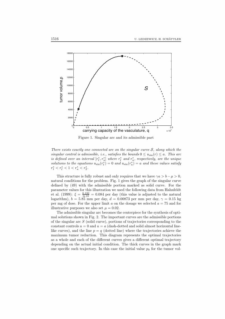
1516 U. LEDZEWICZ, H. SCHÄTTLER
0 0.5 1 1.5 2 2.5 3 3.5
x 104
0
2000
4000
6000
8000
10000
12000
14000
16000
18000
carrying capacity of the vasculature, q
tum
or
volu
me
,p
S
Figure 1. Singular arc and its admissible part
There exists exactly one connected arc on the singular curve S, along which thesingular control is admissible, i.e., satisfies the bounds 0 ≤ usin(r) ≤ a. This arcis defined over an interval [r∗ℓ , r
∗u] where r∗ℓ and r∗u, respectively, are the unique
solutions to the equations usin(r∗
ℓ ) = 0 and usin(r∗u) = a and these values satisfyr∗1 < r∗ℓ < 1 < r∗u < r∗2 .
This structure is fully robust and only requires that we have γa > b−µ > 0,natural conditions for the problem. Fig. 1 gives the graph of the singular curvedefined by (49) with the admissible portion marked as solid curve. For theparameter values for this illustration we used the following data from Hahnfeldtet al. (1999): ξ = 0.192
ln 10 = 0.084 per day (this value is adjusted to the naturallogarithm), b = 5.85 mm per day, d = 0.00873 per mm per day, γ = 0.15 kgper mg of dose. For the upper limit a on the dosage we selected a = 75 and forillustrative purposes we also set µ = 0.02.
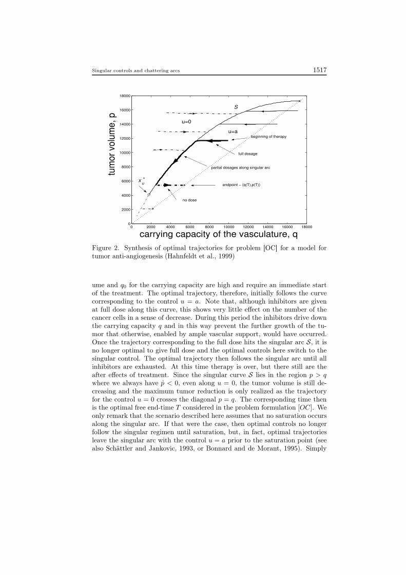
The admissible singular arc becomes the centerpiece for the synthesis of opti-mal solutions shown in Fig. 2. The important curves are the admissible portionsof the singular arc S (solid curve), portions of trajectories corresponding to theconstant controls u = 0 and u = a (dash-dotted and solid almost horizontal line-like curves), and the line p = q (dotted line) where the trajectories achieve themaximum tumor reduction. This diagram represents the optimal trajectoriesas a whole and each of the different curves gives a different optimal trajectorydepending on the actual initial condition. The thick curves in the graph markone specific such trajectory. In this case the initial value p0 for the tumor vol-
Singular controls and chattering arcs 1517
0 2000 4000 6000 8000 10000 12000 14000 16000 180000
2000
4000
6000
8000
10000
12000
14000
16000
18000
carrying capacity of the vasculature, q
tum
or
volu
me
, p
u=0
u=a
S
beginning of therapy
partial dosages along singular arc
no dose
endpoint − (q(T),p(T))
full dosage
x * u
Figure 2. Synthesis of optimal trajectories for problem [OC] for a model fortumor anti-angiogenesis (Hahnfeldt et al., 1999)
ume and q0 for the carrying capacity are high and require an immediate startof the treatment. The optimal trajectory, therefore, initially follows the curvecorresponding to the control u = a. Note that, although inhibitors are givenat full dose along this curve, this shows very little effect on the number of thecancer cells in a sense of decrease. During this period the inhibitors drive downthe carrying capacity q and in this way prevent the further growth of the tu-mor that otherwise, enabled by ample vascular support, would have occurred.Once the trajectory corresponding to the full dose hits the singular arc S, it isno longer optimal to give full dose and the optimal controls here switch to thesingular control. The optimal trajectory then follows the singular arc until allinhibitors are exhausted. At this time therapy is over, but there still are theafter effects of treatment. Since the singular curve S lies in the region p > q
where we always have p < 0, even along u = 0, the tumor volume is still de-creasing and the maximum tumor reduction is only realized as the trajectoryfor the control u = 0 crosses the diagonal p = q. The corresponding time thenis the optimal free end-time T considered in the problem formulation [OC]. Weonly remark that the scenario described here assumes that no saturation occursalong the singular arc. If that were the case, then optimal controls no longerfollow the singular regimen until saturation, but, in fact, optimal trajectoriesleave the singular arc with the control u = a prior to the saturation point (seealso Schättler and Jankovic, 1993, or Bonnard and de Morant, 1995). Simply

1518 U. LEDZEWICZ, H. SCHÄTTLER
continuing the control with u = a is not optimal (Ledzewicz and Schättler,2007).
When a linearmodel forpharmacokinetics is added, themodel being [OCwLDC],the singular curve is preserved as a vertical surface in (p, q, c)-space, Fig. 3, andnow the singular arc is defined as the intersection with the graph of the functionc = ψ(p, q), see Fig. 4.
0
5000
10000
15000
0
5000
10000
15000
0
50
100
150
200
concentr
ation, c
tumor volume, p vascular support, q
Figure 3. Vertical singular surface in (p, q, c)-space for problem [OCwLDC]
0
5000
10000
15000
0
5000
10000
15000
0
50
100
150
200
vascular support, qtumor volume, p
concentr
ation, c
Figure 4. Singular arc in (p, q, c)-space for problem [OCwLDC]
Singular controls and chattering arcs 1519
Chattering arcs now become the prime candidates for the optimal transitionsto and from the singular arc. The precise structure of these optimal controls,however, has not yet been worked out. From a practical point of view, for theunderlying application chattering controls are not realistic. The real signifi-cance of knowing the optimal solution lies rather in establishing a benchmarkvalue with which other, simple and realizable strategies can be compared. Infact, even for problem [OC], the optimal singular controls are defined by time-varying feedback controls and thus are not medically realizable. In Ledzewicz,Marriott, Maurer and Schättler (2009), we have shown for this problem (forboth the original model by Hahnfeldt et al., 1999, and its modification by Er-gun, Camphansen and Wein, 2003) that simple piecewise constant controls withtwo dosages - easily practically realizable protocols - provide excellent subopti-mal approximations to the optimal controls that consistently give values thatcome within 1% of the theoretically optimal values. These dosages are not ofthe bang type, but rather give lower dosages over specified time intervals thatmimick the time-varying optimal singular control in its behavior. It is hopedthat similar results can be established for the problem [OCwLDC] when a linearpharmacokinetic model is added and that simple, non-optimal concatenationswith bang controls will provide satisfactory suboptimal approximations. Thus,it would not only be of theoretical interest to establish an optimal synthesis ofcontrolled trajectories for this problem.
6. Conclusion
We considered a Mayer optimal control problem for a single-input, control affinesystem in dimension 2 when control is replaced by the state of a first order time-invariant linear system. We showed that the fundamental formulas that defineand characterize the optimality of singular controls and their corresponding tra-jectories are preserved verbatim under such an extension. However, the intrinsicorder of the singular arc increases from 1 to 2. If the Kelley condition is sat-isfied and the singular control takes values in the interior of the control set,then this precludes concatenations between the singular and bang controls frombeing optimal and now chattering arcs become the prime candidates to effectthe transitions to and from the singular arc.
For an application of these results to the problem of minimizing the tumorsize for a model of tumor anti-angiogenesis, establishing the structure of anoptimal synthesis would provide valuable information about the extent, to whichthe pharmacokinetics of anti-angiogenic agents would need to be included in themodeling of the problem. In this regard, the important question is how close tooptimal protocols simple realizable ones can come and how the optimal valuesfor the two problem formulations [OC] and [OCwLDC] compare. Thus, if thereis little difference in the tumor volumes achievable with realizable protocols, thisgives credence to a modeling approach that neglects the pharmacokinetic model.

1520 U. LEDZEWICZ, H. SCHÄTTLER
References
Anderson, A. and Chaplain, M. (1998) Continuous and discrete mathe-matical models of tumor-induced angiogenesis. Bull. Math. Biol. 60,857-899.
Arakelyan, L., Vainstain, V. and Agur, Z. (2002) A computer algorithmdescribing the process of vessel formation and maturation, and its use forpredicting the effects of anti-angiogenic and anti-maturation therapy onvascular tumour growth. Angiogenesis 5, 203-214.
Boehm, T., Folkman, J., Browder, T. and O’Reilly, M.S. (1997) An-tiangiogenic therapy of experimental cancer does not induce acquired drugresistance. Nature, 390, 404-407.
Boltyansky, V.G. (1966) Sufficient conditions for optimality and the justifi-cation of the dynamic programming method. SIAM J. Control 4, 326-361.
Bonnard, B. and Chyba, M. (2003) Singular Trajectories and their Rolein Control Theory. Mathématiques & Applications 40, Springer Verlag,Paris.
Bonnard, B. and de Morant, J. (1995) Toward a geometric theory in thetime-minimal control of chemical batch reactors. SIAM J. Control Optim.33, 1279-1311.
Boscain, U. and Piccoli, B. (2004) Optimal Syntheses for Control Systemson 2-D Manifolds. Mathématiques & Applications 43, Springer Verlag,Paris.
Bressan, A. and Piccoli, B. (2007) Introduction to the Mathematical The-ory of Control. American Institute of Mathematical Sciences.
Bryson, Jr., A.E. and Ho, Y.C. (1975) Applied Optimal Control. RevisedPrinting, Hemisphere Publishing Company, New York.
Castiglione, F. and Piccoli, B. (2006) Optimal control in a model of den-dritic cell transfection cancer immunotherapy. Bulletin of MathematicalBiology, 68, 255-274.
Chyba, M. and Haberkorn, T. (2003) Autonomous underwater vehicles:singular extremals and chattering. In: F. Cergioli et al., eds., Systems,Control, Modeling and Optimization. Springer Verlag, 103-113.
Davis, S. and Yancopoulos, G.D. (1999) The angiopoietins: Yin and Yangin angiogenesis. Curr. Top. Microbiol. Immunol., 237, 173-185.
de Pillis, L.G. and Radunskaya, A. (2001) A mathematical tumor modelwith immune resistance and drug therapy: an optimal control approach.J. of Theoretical Medicine, 3, 79-100.
d’Onofrio, A. and Gandolfi, A. (2004) Tumour eradication by antiangio-genic therapy: analysis and extensions of the model by Hahnfeldt et al.Math. Biosci., 191, 159-184.
Eisen, M. (1979) Mathematical Models in Cell Biology and Cancer Chemo-therapy. Lecture Notes in Biomathematics, 30, Springer Verlag.

Singular controls and chattering arcs 1521
Ergun, A., Camphausen, K. and Wein, L.M. (2003) Optimal schedulingof radiotherapy and angiogenic inhibitors. Bull. of Math. Biology, 65,407-424.
Felgenhauer, U. (2003) On stability of bang-bang type controls. SIAM J.Control Optim., 41, (6), 1843-1867.
Fister, K.R. and Panetta, J.C. (2000) Optimal control applied to cell-cycle-specific cancer chemotherapy. SIAM J. Appl. Math., 60, 1059-1072.
Folkman, J. (1972) Antiangiogenesis: new concept for therapy of solid tu-mors. Ann. Surg., 175, 409-416.
Folkman, J. (1995) Angiogenesis inhibitors generated by tumors. Mol. Med.,1, 120-122.
Gardner-Moyer, H. (1973) Sufficient conditions for a strong minimum insingular control problems. SIAM J. Control, 11, 620-636.
Hahnfeldt, P., Panigrahy, D., Folkman, J. and Hlatky, L. (1999) Tu-mor development under angiogenic signaling: a dynamical theory of tu-mor growth, treatment response, and postvascular dormancy. Cancer Re-search, 59, 4770-4775.
Kelley, H.J. (1964) A second variation test for singular extremals. AIAA(American Institute for of Aeronautics and Astronautics) J., 2, 1380-1382.
Kelley, H.J., Kopp, R. and Moyer, H.G. (1967) Singular Extremals. In:G. Leitmann, ed.Topics in Optimization, Academic Press.
Kerbel, R.S. (1997) A cancer therapy resistant to resistance. Nature, 390,335-336.
Kirschner, D., Lenhart, S. and Serbin, S. (1997) Optimal control of che-motherapy of HIV. J. Math. Biol., 35, 775-792.
Klagsburn, M. and Soker, S. (1993) VEGF/VPF: the angiogenesis factorfound? Curr. Biol., 3, 699-702.
Knobloch, H.W. (1981) Higher Order Necessary Conditions in Optimal Con-trol Theory. LNCIS 34, Springer Verlag, Berlin.
Ledzewicz, U., Marriott, J., Maurer, H. and Schättler, H. (2009) Re-alizable protocols for optimal administration of drugs in mathematicalmodels. Mathematical Medicine and Biology, to appear.
Ledzewicz, U., Munden, J. and Schättler, H. (2009) Scheduling of An-giogenic Inhibitors for Gompertzian and Logistic Tumor Growth Models.Discrete and Continuous Dynamical Systems, Series B, to appear.
Ledzewicz, U. and Schättler, H. (2002a) Optimal bang-bang controls fora 2-compartment model in cancer chemotherapy. Journal of OptimizationTheory and Applications - JOTA, 114, 609-637.
Ledzewicz, U. and Schättler, H. (2002b) Analysis of a cell-cycle specificmodel for cancer chemotherapy. J. of Biol. Syst., 10, 183-206.
Ledzewicz, U. and Schättler, H. (2005) The influence of PK/PD on thestructure of optimal control in cancer chemotherapy models. MathematicalBiosciences and Engineering (MBE), 2, (3), 561-578.

1522 U. LEDZEWICZ, H. SCHÄTTLER
Ledzewicz, U. and Schättler, H. (2006) Application of optimal control toa system describing tumor anti-angiogenesis. Proceedings of the 17th In-ternational Symposium on Mathematical Theory of Networks and Systems(MTNS), Kyoto, Japan, July 2006, 478-484.
Ledzewicz, U. and Schättler, H. (2007a) Anti-Angiogenic therapy in can-cer treatment as an optimal control problem. SIAM J. Contr. Optim., 46,1052-1079.
Ledzewicz, U. and Schättler, H. (2007b) Optimal controls for a modelwith pharmacokinetics maximizing bone marrow in cancer chemo-therapy.Mathematical Biosciences, 206, 320-342.
Martin, R.B. (1992) Optimal control drug scheduling of cancer chemother-apy. Automatica, 28, 1113-1123.
Maurer, H., Büskens, C., Kim, J.H. and Kaja, Y. (2005) Optimization te-chniques for the verification of second-order sufficient conditions for bang-bang controls. Optimal Control, Applications and Methods, 26, 129-156.
Piccoli, B. and Sussmann, H. (2000) Regular synthesis and sufficient con-ditions for optimality. SIAM J. on Control and Optimization, 39, 359-410.
Schättler, H. and Jankovic, M. (1993) A Synthesis of time-opti-mal con-trols in the presence of saturated singular arcs. Forum Mathematicum, 5,203-241.
Stefani, G. (2003) On sufficient optimality conditions for singular extremals.Proceedings of the 42nd IEEE Conference on Decision and Control (CDC),Maui, Hi, USA, December 2003, 2746-2749.
Sussmann, H.J. (1982) Time-optimal control in the plane. In: Feedback Con-trol of Linear and Nonlinear Systems, LNCS 39, Springer Verlag, Berlin,244-260.
Sussmann, H.J. (1987) The structure of time-optimal trajectories for single-input systems in the plane: the C∞ nonsingular case. SIAM J. ControlOptim., 25, 433-465.
Swan, G.W. (1988) General applications of optimal control theory in cancerchemotherapy. IMA J. Math. Appl. Med. Biol., 5, 303-316.
Swan, G.W. (1990) Role of optimal control in cancer chemotherapy. Math.Biosci., 101, 237-284.
Swierniak, A. (1988) Optimal treatment protocols in leukemia - modellingthe proliferation cycle. Proceedings of the 12th IMACS World Con-gress,Paris, 4, 170-172.
Swierniak, A. (1995) Cell cycle as an object of control. J. of BiologicalSystems, 3, 41-54.
Swierniak, A. (2008) Direct and indirect control of cancer populations. Bul-letin of the Polish Academy of Sciences, Technical Sciences, 56, 367-378.
Swierniak, A., Gala, A., d’Onofrio, A. and Gandolfi, A. (2006) Op-timization of angiogenic therapy as optimal control problem. In: M.Doblare, ed., Proceedings of the 4th IASTED Conference on Biomechan-ics, Acta Press, 56-60.

Singular controls and chattering arcs 1523
Swierniak, A., Ledzewicz, U. and Schättler, H. (2003) Optimal controlfor a class of compartmental models in cancer chemotherapy. Int. J. Ap-plied Mathematics and Computer Science, 13, 357-368.
Swierniak,A., Polanski,A. and Kimmel,M. (1996) Optimal control prob-lems arising in cell-cycle-specific cancer chemotherapy. Cell Proliferation,29, 117-139.
Zelikin, M.I. and Borisov, V.F. (1994) Theory of Chattering Control withApplications to Astronautics, Robotics, Economics and Engineering. Bir-khäuser.
Zelikin, M.I. and Zelikina, L.F. (1998) The structure of optimal synthesisin a neighborhood of singular manifolds for problems that are affine incontrol. Sbornik: Mathematics, 189, 1467-1484.