Singly-Bordered Block-Diagonal Form for Minimal Problem...

Singly-Bordered Block-Diagonal Form forMinimal Problem Solvers

Zuzana Kukelova1,2, Martin Bujnak3, Jan Heller1, and Tomas Pajdla1

1Czech Technical University in Prague, 166 27 Praha 6, Technicka 2, Czech Republic2Microsoft Research Ltd, 21 Station Road, Cambridge CB1 2FB, UK

3Capturing Reality s.r.o., Bratislava, Slovakia

Abstract. The Grobner basis method for solving systems of polynomialequations became very popular in the computer vision community as ithelps to find fast and numerically stable solutions to difficult problems.In this paper, we present a method that potentially significantly speedsup Grobner basis solvers. We show that the elimination template matri-ces used in these solvers are usually quite sparse and that by permutingthe rows and columns they can be transformed into matrices with niceblock-diagonal structure known as the singly-bordered block-diagonal(SBBD) form. The diagonal blocks of the SBBD matrices constitute in-dependent subproblems and can therefore be solved, i.e. eliminated orfactored, independently. The computational time can be further reducedon a parallel computer by distributing these blocks to different processorsfor parallel computation. The speedup is visible also for serial processingsince we perform O(n3) Gauss-Jordan eliminations on smaller (usuallytwo, approximately n

2× n

2and one n

3× n

3) matrices. We propose to com-

pute the SBBD form of the elimination template in the preprocessingoffline phase using hypergraph partitioning. The final online Grobnerbasis solver works directly with the permuted block-diagonal matricesand can be efficiently parallelized. We demonstrate the usefulness of thepresented method by speeding up solvers of several important minimalcomputer vision problems.

1 Introduction

The Grobner basis method for solving systems of polynomial equations wasrecently used to solve many important computer vision problems [2, 7, 19, 3, 24,25]. This method became popular for creating efficient specific solvers to minimalproblems and even an automatic generator for creating source codes of suchminimal Grobner basis solvers was proposed in [18].

Minimal solvers, such as the 5-point relative pose solver [22, 25] or the P4Pfabsolute pose solver [2], are often used inside a RANSAC [12] loop and areparts of large systems like SfM pipelines or recognition systems. Maximizing theefficiency of these solvers is therefore highly important.

Grobner basis solvers usually consist of two separate steps. In the first stepGauss-Jordan (G-J) elimination, QR, or LU decomposition of one or several

2 Zuzana Kukelova, Martin Bujnak, Jan Heller, Tomas Pajdla

matrices created using the so-called elimination templates [18] is performed. Inthe second step the solutions are extracted from the eigenvalues and eigenvectorsof a multiplication (action) matrix [23] .

Recently, several papers addressed the numerical stability and the speed ofGrobner basis solvers [5, 8, 6, 18, 21, 4]. In [5, 8, 6], it has been shown that the nu-merical stability of Grobner basis solvers can be improved by reordering columnsin the elimination templates using QR or LU decompositions or by “basis ex-tension”. Several methods for reducing the size of the elimination templates inorder to speed up the Grobner basis solvers were presented in [21, 18].

Most recently, two methods that speed up the second step of Grobner basissolvers, i.e. the eigenvalue computations, were proposed in [4]. The first methodis based on a modified matrix FGLM algorithm for transforming Grobner basesand results in a single-variable polynomial which roots are efficiently computedonly on a certain feasible interval using Sturm-sequences. The second method isbased on fast calculation of the characteristic polynomial of an action matrix,again solved using Sturm-sequences. Both methods are in fact equivalent andcan be used to significantly speed up the second step of Grobner basis solvers.

In this paper, we present a method that can significantly speed up the firststep of Grobner basis solvers, i.e. G-J elimination, QR, or LU decompositionof matrices from the elimination templates. We observe that these eliminationtemplate matrices are usually quite sparse and by permuting the rows and thecolumns they can be transformed into matrices with an agreeable block-diagonalstructure. The diagonal blocks of such permuted matrices constitute indepen-dent subproblems and as such can be solved, i.e. eliminated or factored, indepen-dently. The computational time can then be reduced on a parallel computer bydistributing these blocks to different processors and by performing the compu-tation in parallel. This speedup is also noticeable on single-threaded computersbecause O(n3) G-J eliminations on smaller (for the presented problems on two,approximately n

2 × n2 and one n

3 × n3 ) matrices is performed.

To obtain a reasonable speed-up, each block in the permuted matrix shouldcontain comparable number of entries, i.e. some balance criterion should be main-tained, and it should be as independent as possible from other blocks. For thispurpose, we permute sparse rectangular matrices from the elimination templatesinto a singly-bordered block-diagonal (SBBD) form with minimum border sizewhile maintaining a given balance criterion on the diagonal blocks.

The problem of permuting sparse matrices into SBBD form is usually for-mulated as hypergraph partitioning [1]. In this paper, we use state-of-the-arthypergraph partitioning tool PaToH [9] that uses multilevel hypergraph parti-tioning approaches based on Kernighan-Lin and Fiduccia-Mattheyses (KLFM)algorithms [11].

The use of row and column permutations to speed up computations is well-known in linear algebra and has been previously exploited in computer visionapplications. For instance, in the bundle adjustment problem, one may transformthe involved sparse matrices into arrowhead or block tridiagonal matrices [26, 20].

Singly-Bordered Block-Diagonal Form for Minimal Problem Solvers 3

However, such transformations are dependent on individual problem instancesand therefore are not used widely in bundle adjustment.

On the other hand, in the proposed method the permutation of an elimi-nation template matrix into SBBD form can be computed offline once for eachtype of minimal problem and applied to all instances. The final online Grobnerbasis solvers work directly with the permuted block-diagonal matrices and caneliminate the diagonal blocks independently and perform the computations inparallel. Moreover, the proposed method can be used along with the methodsfrom [4] that speed up the second step of Grobner basis solvers.

We demonstrate the usefulness of the presented approach by speeding upsolvers of several important minimal computer vision problems.

Next, we briefly describe the Grobner basis method for solving systems ofpolynomial equations and the process of generating Grobner basis solvers.

2 Grobner basis method

Grobner basis method for solving systems of polynomial equations became verypopular in the computer vision community since it helps to find fast and numer-ically stable solutions to difficult problems.

Letf1(x) = 0, . . . , fm(x) = 0 (1)

be a system of m polynomial equations in n unknowns x = (x1, . . . , xn) thatwe want to solve and let this system have a finite number of solutions. Thepolynomials f1, ..., fm define an ideal I = {Σm

i=1fi hi |hi ∈ C [x1, ..., xn]}, whichis a set of all polynomials that can be generated as polynomial combinations ofthe initial polynomials f1, ..., fm. In general, an ideal can be generated by manydifferent sets of generators which all share the same set of solutions. There isa special set of generators though, the reduced Grobner basis w.r.t. the lexico-graphic ordering, which generates the ideal I but is easy (often trivial) to solveat the same time [10].

Unfortunately, computing the Grobner basis w.r.t. the lexicographic orderingfor larger systems of polynomial equations, and therefore for the most computervision problems, is often not feasible.

Therefore, Grobner basis solvers usually construct a Grobner basis G undera different ordering, e.g. the graded reverse lexicographic (grevlex) ordering,which is often easier to compute. This Grobner basis G is then used to constructa special multiplication matrix Mp [23], also called the “action matrix”. Let A

be the quotient ring A = C [x1, ..., xn] /I [10] and B ={xα|xαG

= xα}

its

monomial basis, where xα = xα11 xα2

2 ...xαnn and xαG

is the remainder of xα afterthe division by a Grobner basis G. Then the action matrix Mp is the matrix ofa linear operator Tp : A → A performing multiplication by a suitably chosenpolynomial p in A w.r.t. the basis B.

The action matrix Mp can be viewed as a generalization of the companionmatrix used in solving one polynomial equation in one unknown [10], since the


solutions to our system of polynomial equations (1) can be obtained from theeigenvalues and eigenvectors of this action matrix.

3 Grobner basis solvers

Many polynomial problems in computer vision share the convenient propertythat the monomials which appear in the set of initial polynomials (1) are, upto the concrete coefficients arising from non-degenerate image measurements,always identical. Thanks to this property, it is not necessary to use generalalgorithms [10] for computing Grobner bases for solving these problems. Usu-ally, specific Grobner basis solvers that can efficiently solve all non-degenerateinstances of a given problem are used in computer vision.

The process of creating these specific Grobner basis solvers consist of twodifferent phases. In the first “offline” phase, so-called “elimination templates”are found. These templates say which input polynomials should be multipliedwith which monomials and then eliminated to obtain all polynomials from thegrevlex Grobner basis or at least all polynomials necessary for constructing anaction matrix. For a one concrete problem, this phase is performed only once.

The second “online” phase consists of two steps. In the first step, the pre-computed elimination templates are filled with specific coefficients arising fromimage measurements and eliminated using G-J elimination to construct the ac-tion matrix. Then, eigenvalues and eigenvectors of this action matrix are usedto find solutions to the initial polynomial equations.

It was shown in [4], that the second step of the online solver can be sped upby replacing the eigenvalue computations with the computations of the charac-teristic polynomial of the action matrix and by efficiently finding roots of thispolynomial using Sturm-sequences.

In this paper, we will show that at the cost of some preprocessing performedin the offline phase we can significantly speed up also the first step of onlineGrobner basis solvers, i.e., G-J elimination, QR, or LU decomposition of matricesfrom the elimination templates.

Elimination templates are created in the offline phase by multiplying initialpolynomials with monomials. Since we are multiplying polynomials by monomi-als only, the new generated polynomials have the same number of monomials asthe polynomials from which they are created.

In the matrix representation of polynomials that is used in the eliminationtemplate, the rows of the matrix correspond to the individual polynomials andthe columns to the monomials. This means that we are effectively only shiftingthe coefficients in this matrix when generating a new polynomial by multiplyingsome initial polynomial fi by a monomial. A new row that corresponds to thenew polynomial contains the same entries as the row corresponding to fi, but indifferent columns. Therefore, the elimination template matrices are usually quitesparse. We will show that in these situations we can permute the rows and thecolumns of these matrices in the preprocessing offline phase and in this way creatematrices that have a nice block-diagonal structure known as the singly-bordered


block diagonal (SBBD) form. The diagonal blocks of such SBBD matrices canthen be eliminated or factored using LU or QR decomposition independently.The computational time can be significantly reduced by distributing these blocksto different processors and by performing the computations in parallel. Moreover,

there is speedup from approximately n3 to (k+1)·(nk

)3, even for serial processing

of an SBBD matrix with k well balanced blocks.Since the permutation matrices that transform the elimination template ma-

trix to the SBBD form are computed in the offline phase, the time spent com-puting these permutation matrices doesn’t influence the speed of the final onlinesolver. Moreover, the computational cost of finding the permutation matrices(for the presented solvers less than 0.1s) is comparable or even lower than thecomputational time of the remaining steps of the offline phase.

4 Sparse Matrix Partitioning

In this section, we describe the singly-bordered block-diagonal form and the wayhow to transform a given matrix to this form.

4.1 Singly-Bordered Block-Diagonal Form

Our goal is to permute the rows and the columns of an m × n sparse matrix A

into a k-way singly-bordered block-diagonal form

ASB = PrAP⊤c =

A11 B1

A22 B2. . .

...Akk Bk

, (2)

where Pr and Pc are, respectively, the row and the column permutation matricesto be determined, k is the pre-defined number of blocks, A11, . . . , Akk are rectan-

gular matrices and B =(B⊤1 . . . B⊤k

)⊤is m× nc border submatrix. Columns of B

are sometimes called the coupling columns.In our case, we want to permute matrix A into an SBBD form ASB (2) such

that the number of coupling columns nc is minimized while a given balancedcriterion is satisfied, i.e. each block Ajj , j = 1, . . . , k of the permuted matrixASB contains comparable number of entries.

Using hypergraph model for sparse matrices, the problem of permuting asparse matrix to SBBD form (2) reduces to the well-known hypergraph parti-tioning problem [1].

Next, we describe hypergraphs and hypergraph partitioning to a level perti-nent to this work.

4.2 Hypergraph partitioning

A hypergraph H = (V,N ) is defined as a set of vertices V and a set of nets (orhyperedges) N , where every net ni ∈ N is a subset of vertices, i.e. ni ⊆ V.


Definition 1. Given a hypergraph H = (V,N ), Π = {V1, . . . ,Vk} is a k-waypartition of H, if the following holds:

1. Vj = ∅, Vj ⊆ V, for 1 ≤ j ≤ k, i.e. each part Vj is nonempty subset of V,2. Vi ∩ Vj = ∅ for all 1 ≤ i ≤ j ≤ k, i.e. parts are pairwise disjoint,

3.∪k

j=1 Vj = V, i.e. the union of all k parts is equal to V.

As in the case of graphs, we can associate weights with hypergraph vertices.Let us denote w (v) the weight associated with a vertex v. Now, we can definethe weight of a set of vertices S as

W (S) =∑v∈S

w (v) . (3)

The partition Π = {V1, . . . ,Vk} is said to be balanced for a given ϵ ≥ 0, ifeach part Vj satisfies the balance criterion

W (Vj)

Wavg≤ 1 + ϵ, j = 1, . . . , k, (4)

where W (Vj) is the weight (3) of a part Vj and Wavg = W (V)k .

Let NS be the set of all nets (hyperedges) that connect more than one partof a partition Π in H. This means that all nets nj ∈ NS have at least one vertexin more than one part Vi ∈ Π. Such nets nj ∈ NS are called cuts or externalnets.

Nets that connect only one part Vi ∈ Π, i.e. they have all vertices in thispart, are called internal nets of part Vi. Let us denote the set of all internal netsof a part Vi as Ni, i = 1, . . . , k. Then, the k-way partition Π = {V1, . . . ,Vk} thatis defined on the vertex set V can also be considered as a (k + 1)-way partitionΠ = {N1, . . . ,Nk;NS} on the net set N . The set NS can be considered as a netseparator whose removal gives k disconnected vetrex parts V1, . . . ,Vk as well ask disconnected net parts N1, . . . ,Nk.

The goal of partitioning is to minimize a cost function called cutsize definedover the external nets NS . Let c (n) denote the cost associated with the netn ∈ N . Then a cost function can be defined as

χ(Π) =∑

nj∈NS

c (nj) . (5)

In our problem of transforming a matrix to an SBBD form all nets have unitcosts, i.e., c (n) = 1 for all n ∈ N and therefore the cost function has very simpleform

χ(Π) =∑

nj∈NS

1 = |NS | . (6)

The hypergraph partitioning problem can be defined as a problem of dividingvertex set V of a hypergraph H into k parts, i.e. a problem of finding a k-way


A =

n1 n2 n3 n4 n5 n6 n7 n8

v1 • • • •v2 • • •v3 • • •v4 • •v5 • •v6 • • •

n8 n1

n3 n4 n7 n6n5 n2

v1

v5 v6 v3

v2

v4

Fig. 1. A 6× 8 matrix A (Left) and its column-net hypergraph representation (Right);symbol “•” represents a nonzero entry of the matrix A.

partition Π = {V1, . . . , Vk}, such that the cost (5) is minimized while the balancecriterion (4) is fulfilled for a given ϵ:

Given H = (V,N ) , ϵ,find Π = argmin

∑nj∈NS

c (nj) ,

Π = {V1, . . . ,Vk} = {N1, . . . ,Nk;NS}subject to

W (,Vj)Wavg

≤ 1 + ϵ, j = 1, . . . , k.

Unfortunately, the hypergraph partitioning problem is known to be NP-hard [13].

4.3 Matrix partitioning

An m × n matrix A = (aij) can be represented as a hypergraph HA = (V,N ).In the column-net hypergraph model, HA contains m vertices and n nets (hy-peredges), i.e. there exists one vertex vi ∈ V for each row i of A and one netnj ∈ N for each column j of A. In this model, the net nj ⊆ V contains verticescorresponding to the rows that have nonzero entry in column j, i.e. vi ∈ nj ifand only if aij = 0. This means that the degree of the vertex vi is equal to thenumber of nonzero entries in row i of A and the size of the net nj is equal to thenumber of nonzero entries in column j of A.

Figure 1 (Left) shows an example of a 6 × 8 matrix A and its column-nethypergraph representation (Right).

Using the hypergraph representation of the matrix A, the problem of trans-forming A to SBBD form ASB (2) can be cast as a hypergraph partitioningproblem in which the cost (6) is equal to the number of coupling columns nc inASB . This claim can be formalized as theorem [1]:

Theorem 1. Let HA = (V,N ) be the hypergraph representation of the matrixA. A k-way partition Π = {V1, . . . ,Vk} = {N1, . . . ,Nk;NS} of HA gives a per-mutation of A to SBBD form ASB (2), where vertices in Vi represent the rowsand the internal nets in Ni the columns of the ith diagonal block of ASB, andexternal nets in NS represent the coupling columns of ASB. Therefore,

– minimizing the cutsize (6) minimizes the number of coupling columns, and– if the criterion (4) is satisfied, then the diagonal submatrices are balanced.


A =

N1 N2 N1 NS N2 N2 NS N1

V1 • • • •V2 • • •V2 • • •V2 • •V1 • •V1 • • •

ASB =

n1 n3 n8 n2 n5 n6 n4 n7

v1 • • • •v5 • •v6 • • •v2 • • •v3 • • •v4 • •

Fig. 2. (Left) 2-way partitioning Π = {V1,V2} = {N1,N2;NS} of HA. (Right) SBBDform ASB of A induced by Π.

Figure 2 (Left) shows a 2-way partitioning Π = {V1,V2} = {N1,N2;NS} of thematrix HA from Figure 1 and its SBBD form ASB induced by Π (Right).

5 Experiments

To demonstrate the usefulness of the presented approach, we used this method tospeed up solvers of three important minimal relative and absolute pose problems.Even though these problems have been previously solved using the Grobner basismethod [18], the large elimination templates connected with these problemsmade the respective solvers relatively slow.

For each of these Grobner basis solvers, we have precomputed the permu-tation matrices that transform the elimination template matrix into an SBBDform. We have formulated the problem of permuting the sparse matrix into anSBBD form as the hypergraph partitioning problem (see Section 4.3) and wehave used the state-of-the-art hypergraph partitioning tool PaToH [9] to solvethis problem. From PaToH, we have received the permutation matrices that wehave used to permute the rows and the columns of the matrix from the elimina-tion template.

Since PaToH uses heuristics for solving the hypergraph partitioning and eachtime returns a slightly different result, we have run this partitioning tool severaltimes for every elimination template matrix. We have obtained reasonable andstable partitions from PaToH for all tested minimal solvers. In all PaToH runs,for the same elimination template matrix, PaToH returned very similar resultswith a similar number of coupling columns (+/- 5). We have selected the ”bestpartitioning” as the partitioning with the smallest number of coupling columns(border) among all runs. For each problem, we have computed the permutationmatrices only once in the preprocessing offline phase.

The difference between the new online Grobner basis solvers and the orig-inal Grobner basis solvers is that the new solvers work directly with the per-muted block-diagonal matrices and therefore perform smaller G-J eliminationsand moreover can be parallelized.

Since the numerical stability of the new solvers is similar to the numericalstability of the state-of-the-art solvers, in this section, we compare only the speedof the solvers.


Further, because all of the solvers are algebraically equivalent, we have evalu-ated them on synthetic noise free data only. In our experiments and performancetests, we executed each algorithm 10K times on synthetically generated data. Allscenes in these experiments were generated using 3D points randomly distributedin a 3D cube. Each 3D point was projected by cameras with random yet feasibleorientations and positions and with random or fixed focal lengths. In the case ofradial distortion problems, radial distortion generated by one-parameter divisionmodel was added to all image points to generate noiseless distorted points.

Next, we describe three minimal problems, the existing Grobner basis solversas well as the new SBBD solutions we based on these solvers, and the gainedspeed-up.

5.1 9-point relative pose different radial distortion problem

Omnidirectional cameras and wide angle lenses are often used in computer vi-sion applications. In fact, not only wide angle lenses but virtually all consumercamera lenses suffer from some amount of radial distortion. Ignoring this typeof distortion, even for standard cameras, may lead to significant errors in 3Dreconstruction, metric image measurements, or in camera calibration.

The first problem that we have studied is the problem of simultaneous es-timation of the fundamental matrix and two radial distortion parameters fortwo uncalibrated cameras with different radial distortions from nine image pointcorrespondences. This problem is useful in applications where images of onescene have been taken by two different cameras, for example by a standard dig-ital camera and by a camera with a wide angle lens or by an omnidirectionalcamera.

This 9-point distortion problem can be after some manipulation of equationsformulated as a system of four equations in four unknowns. Several Grobnerbasis solutions to this problem exist [19, 18]. The solution [18] which results inthe smallest elimination template, performs G-J elimination of a 179×203 matrixand extracts 24 solutions from the eigenvalues and eigenvectors of a 24×24 actionmatrix.

The large 179×203 elimination template matrix makes the 9-point distortionsolver [18] relatively slow and not very useful in real applications. However, wewill show that this elimination template matrix can be transformed to a matrixin SBBD form and therefore the computational time of G-J elimination can besignificantly reduced.

SBBD form For the 9-point distortion solver, as well as for the two remainingstudied minimal solvers, we have obtained the best results, i.e. the smallestnumber of the coupling columns and a well balanced blocks in SBBD matrix (2),for two blocks.

First, we have removed the last 24 columns of the 179×203 elimination tem-plate matrix M from the state-of-the-art solver [18]. These columns correspondto the basis B of the quotient ring A = C [x1, ..., xn] /I and should not be per-muted and eliminated. Then, we have used the square 179 × 179 matrix as the


0 50 100 150 200

0

20

40

60

80

100

120

140

160

180

nz = 2462

0 50 100 150 200

0

20

40

60

80

100

120

140

160

180

nz = 2462

0 50 100 150 200

0

20

40

60

80

100

120

140

160

180

nz = 9339

Fig. 3. 9-point radial distortion problem: (Left) the input 179× 203 eliminationtemplate matrix. (Center) The SBBD form of this matrix found by PaToh for k = 2.The black dash-dot lines separate the independent blocks and the coupling columnswith the red dash-dot line separating the last 24 basis columns. (Right) A matrixobtained after two independent G-J eliminations of the two blocks of ASB .

input to the hypergraph partitioning tool PaToH [9]. We set the weights to 1and the PaToH imbalance ratio to 3%. These are the deafult values for PaToHand worked well for all studied solvers.

Figure 3 shows the input 179 × 203 elimination template matrix (Left) andits SBBD form found by PaToh for k = 2 (Center). In this case, the size of thefirst block A11 in ASB (2) is 90×47, the size of the second block A22 is 89×57 andthe number of the coupling columns nc together with the 24 basis columns is 99.The diagonal block matrices A11 and A22 are independent and can be thereforeeliminated separately.

Figure 3 (Right) shows the matrix Mr that we have obtained after two separateG-J eliminations of the rows of ASB that correspond to A11 and A22. In this case,we have permuted the eliminated rows such that the identity matrix is at thetop left corner.

After performing these two separate eliminations, it is sufficient to performG-J elimination of the bottom right 75× 99 submatrix of Mr. It is not necessaryto eliminate all rows of Mr above this bottom submatrix. To create the actionmatrix, we only need four from the first 104 rows and therefore it is sufficient toeliminate only these four rows from the top 104 rows of Mr.

5.2 P4P+f problem

The second problem is the problem of estimating the absolute pose of a camerawith unknown focal length from four 2D-3D point correspondences. This problemresults in five equations in four unknowns and has ten solutions [2]. The P4P+fproblem is very important in real Structure-from-Motion pipelines and thereforethe efficiency of its solver is crucial.

As the basis of our method we have used the state-of-the art P4P+f solverdownloaded from the webpage [16]. This solver performs G-J elimination of an78×88 elimination template matrix and extracts solutions from a 10×10 actionmatrix.


0 20 40 60 80

0

10

20

30

40

50

60

70

nz = 736

0 20 40 60 80

0

10

20

30

40

50

60

70

nz = 736

0 20 40 60 80

0

10

20

30

40

50

60

70

nz = 1255

Fig. 4. P4P+f problem: (Left) the input 78×88 elimination template matrix. (Cen-ter) The SBBD form of this matrix found by PaToh for k = 2. The black dash-dot linesseparate the independent blocks and the coupling columns and the red dash-dot lineseparate the last 10 basis columns. (Right) A matrix obtained after two independentG-J eliminations of the two blocks of ASB .

SBBD form For the P4P+f solver, we have precomputed in the offline phasethe 2-block SBBD form ASB (2) of its 78 × 88 elimination template matrix.As for the 9-point distortion problem, we have fixed the last 10 columns thatcorrespond to the basis B of the quotient ring A and run PaToH on a square78× 78 matrix.

Figure 4 shows the input 78× 88 elimination template matrix of the P4P+fsolver (Left) and its SBBD form ASB found by PaToh for k = 2 (Center). In thiscase, we have obtained nice blocks of size 37× 24 and 41× 35, and a relativelysmall number of coupling columns nc = 19. This means that together with 10basis columns we have obtained a border of size 29.

Figure 4 (Right) shows the matrix Mr which we have obtained after twoseparate G-J eliminations of the first 37 and the last 41 rows of the SBBDmatrix ASB . We have again permuted the eliminated rows such that the identitymatrix is in the top left corner.

After performing the two independent eliminations, it is sufficient to performG-J elimination of the bottom right 19 × 29 submatrix of Mr. Again, it is notnecessary to eliminate all rows of Mr above this submatrix. To create the actionmatrix, it is sufficient to eliminate only four rows from the top 59 rows of Mr.

5.3 P4P+f+r problem

The last problem that we have solved is the problem of estimating the absolutepose of a camera with unknown focal length and unknown radial distortion fromfour 2D-3D point correspondences. As shown in [15], the consideration of radialdistortion in absolute pose solvers may bring a significant improvement in manyreal world applications. The general formulation of this problem [15] results infive equations in five unknowns and in a quite large and impractical solver (a1134 x 720 matrix) with 24 solutions. The final solver runs in about 70ms.

A more practical solution to the P4P+f+r problem was proposed in [3]. Bydecomposing the problem into a nonplanar and planar cases, much simpler and


0 50 100 150

0

20

40

60

80

100

120

nz = 1940

0 50 100 150

0

20

40

60

80

100

120

nz = 1940

0 50 100 150

0

20

40

60

80

100

120

nz = 4545

Fig. 5. P4P+f+r problem: (Left) the input 136× 152 elimination template matrix.(Center) The SBBD form of this matrix found using PaToh for k = 2. The blackdash-dot lines separate the independent blocks and the coupling columns, the reddash-dot line separates the last 16 basis columns. (Right) A matrix obtained after twoindependent G-J eliminations of the two blocks of ASB .

efficient solvers were obtained. The planar solver is quite simple and performsG-J elimination of a 12×18 matrix. The solution to the non-planar case requiresto perform G-J elimination of a 136×152 matrix and the eigenvalue computationof a 16× 16 matrix. The non-planar solver from [3] was used as the input of ournew method.

SBBD form The non-planar P4P+f+r solver [3] has 16 solutions. We havefirst reordered the columns of the 136× 152 elimination template matrix of thissolver, such that the columns corresponding to the 16 dimensional basis B of thequotient ring A were at the end of this matrix. Then, we have fixed these last 16columns and executed the hypergraph partitioning tool PaToH [9] on the square136 × 136 matrix. Again, we have set the weights to 1, the number of requiredblocks to 2, and the imbalance ratio to 3%.

The input 136×152 elimination template matrix for the P4P+f+r solver canbe seen in Figure 5 (Left) and its SBBD form ASB found by PaToH for k = 2in Figure 5 (Center). In this SBBD matrix ASB , the size of the first block A11is 68 × 45, the size of the second block A22 is 68 × 44, and the number of thecoupling columns nc together with the 16 fixed basis columns is 63.

Figure 5 (Right) shows the matrix Mr that has been obtained after two sepa-rate G-J eliminations of the first 68 and the last 68 rows of the SBBD matrix ASB

and after the permutation of the eliminated rows such that the identity matrix isat the top left corner. Again, these two blocks can be eliminated independently.

After performing these two independent eliminations it is sufficient to per-form G-J elimination of the bottom right 47× 63 submatrix of Mr. In this case,we need the eight of the first 89 rows to create the action matrix. Therefore, inthe final step it it sufficient only to eliminate these eight rows from the top 89rows of Mr.


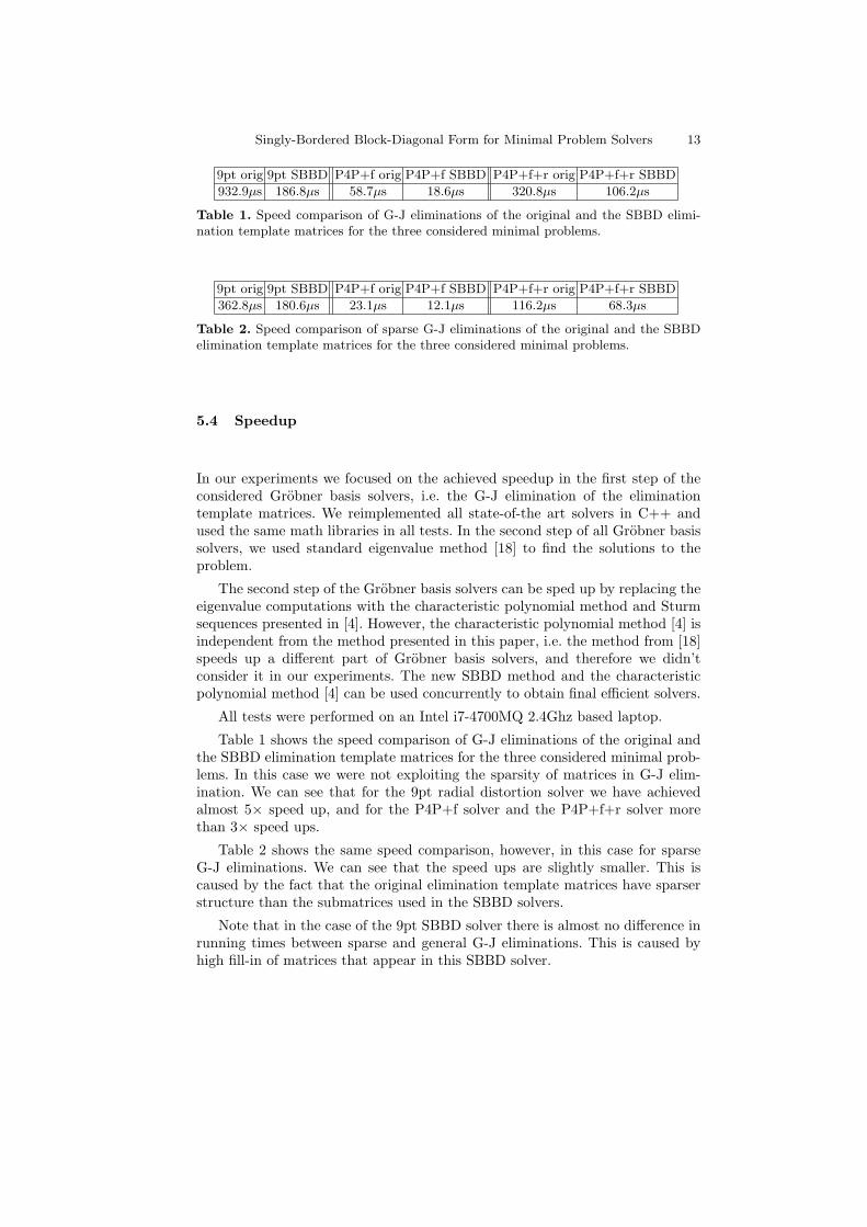
9pt orig 9pt SBBD P4P+f orig P4P+f SBBD P4P+f+r orig P4P+f+r SBBD

932.9µs 186.8µs 58.7µs 18.6µs 320.8µs 106.2µs

Table 1. Speed comparison of G-J eliminations of the original and the SBBD elimi-nation template matrices for the three considered minimal problems.

9pt orig 9pt SBBD P4P+f orig P4P+f SBBD P4P+f+r orig P4P+f+r SBBD

362.8µs 180.6µs 23.1µs 12.1µs 116.2µs 68.3µs

Table 2. Speed comparison of sparse G-J eliminations of the original and the SBBDelimination template matrices for the three considered minimal problems.

5.4 Speedup

In our experiments we focused on the achieved speedup in the first step of theconsidered Grobner basis solvers, i.e. the G-J elimination of the eliminationtemplate matrices. We reimplemented all state-of-the art solvers in C++ andused the same math libraries in all tests. In the second step of all Grobner basissolvers, we used standard eigenvalue method [18] to find the solutions to theproblem.

The second step of the Grobner basis solvers can be sped up by replacing theeigenvalue computations with the characteristic polynomial method and Sturmsequences presented in [4]. However, the characteristic polynomial method [4] isindependent from the method presented in this paper, i.e. the method from [18]speeds up a different part of Grobner basis solvers, and therefore we didn’tconsider it in our experiments. The new SBBD method and the characteristicpolynomial method [4] can be used concurrently to obtain final efficient solvers.

All tests were performed on an Intel i7-4700MQ 2.4Ghz based laptop.

Table 1 shows the speed comparison of G-J eliminations of the original andthe SBBD elimination template matrices for the three considered minimal prob-lems. In this case we were not exploiting the sparsity of matrices in G-J elim-ination. We can see that for the 9pt radial distortion solver we have achievedalmost 5× speed up, and for the P4P+f solver and the P4P+f+r solver morethan 3× speed ups.

Table 2 shows the same speed comparison, however, in this case for sparseG-J eliminations. We can see that the speed ups are slightly smaller. This iscaused by the fact that the original elimination template matrices have sparserstructure than the submatrices used in the SBBD solvers.

Note that in the case of the 9pt SBBD solver there is almost no difference inrunning times between sparse and general G-J eliminations. This is caused byhigh fill-in of matrices that appear in this SBBD solver.


6 Conclusion

In this paper, we have shown that the elimination template matrices used inpopular Grobner basis solvers are usually quite sparse and that by permutingtheir rows and columns can be transformed into matrices with a nice block-diagonal structure known as the singly-bordered block-diagonal (SBBD) form.The permutation of an elimination template matrix into the SBBD form canbe computed in the preprocessing offline phase using hypergraph partitioning.Therefore, the time for finding the permutation matrices doesn’t influence thespeed of the final online Grobner basis solver.

The final online Grobner basis solver works directly with the permuted SBBDmatrices. The computational cost of the first step of these Grobner basis solversis significantly reduced since we perform O(n3) G-J eliminations on smaller (forthe presented solvers usually two approximately n

2 ×n2 and one n

3 ×n3 ) matrices.

Moreover, two of these three G-J eliminations can be performed independentlyand therefore parallelized. We have demonstrate the usefulness of the presentedmethod by speeding up several important minimal computer vision solvers.

Acknowledgement This work has been supported by the EC under projectPRoViDE FP7-SPACE-2012-312377.

References

1. C. Aykanat, A. Pinar, U. V. Catalyurek, Permuting Sparse Rectangular Matricesinto Block-Diagonal Form. SIAM Journal on Scientific Computing, 12/2002.

2. M. Bujnak, Z. Kukelova, T. Pajdla, A general solution to the P4P problem forcamera with unknown focal length. CVPR 2008.

3. M. Bujnak, Z. Kukelova, and T. Pajdla. New efficient solution to the absolute poseproblem for camera with unknown focal length and radial distortion. ACCV 2010.

4. M. Bujnak, Z. Kukelova, T. Pajdla, Making minimal solvers fast. CVPR 2008.5. M. Byrod, K. Josephson, and K. Astrom. Improving numerical accuracy of Grobner

basis polynomial equation solver. ICCV 2007.6. M. Byrod, K. Josephson, and K. Astrom. A Column-Pivoting Based Strategy for

Monomial Ordering in Numerical Grobner Basis Calculations. ECCV 2008.7. M. Byrod, M. Brown, and K. Astrom. Minimal Solutions for Panoramic Stitching

with Radial Distortion. BMVC 2009.8. M. Byrod. Numerical Methods for Geometric Vision: From Minimal to Large Scale

Problems. PhD Thesis, Centre for Mathematical Sciences, Lund University , 2010.9. U.V. Catalyurek, C. Aykanat. PaToH: Partitioning Tool for Hypergraphs, Version

3.1, 2011.10. D. Cox, J. Little, and D. O’Shea. Using Algebraic Geometry, Second edition, volume

185. Springer Verlag, Berlin - Heidelberg - New York, 2005.11. C. M. Fiduccia and R. M Mattheyses. A linear-time heuristic for improving

network partitions. 19th ACM/IEEE Design Automation Conference, 1982.12. M. A. Fischler and R. C. Bolles. Random Sample Consensus: A paradigm for model

fitting with applications to image analysis and automated cartography. Comm.ACM, 24(6):381–395, (1981).


13. M. Garey, D. Johnson, and L. Stockmeyer. Some Simplified NP-Complete GraphProblems, Theoretical Computer Science, vol. 1, 1976.

14. D. Hook, P. McAree, Using Sturm Sequences To Bracket Real Roots of PolynomialEquations, Graphic Gems I, Academic Press, 416-423, 1990.

15. K. Josephson and M. Byrod. Pose estimation with radial distortion and unknownfocal length. In CVPR09, 2009.

16. http://cmp.felk.cvut.cz/minimal/17. K. Kuehnle and E. Mayr. Exponential space computation of Groebner bases. In

Proceedings of ISSAC. ACM, 1996.18. Z. Kukelova and M. Bujnak and T. Pajdla. Automatic Generator of Minimal

Problem Solvers. ECCV 2008.19. Z. Kukelova, M. Byrod, K. Josephson, T. Pajdla, K. Astrom. Fast and robust

numerical solutions to minimal problems for cameras with radial distortion. Com-puter Vision and Image Understanding, Vol. 114, No. 2, pp 234-244, (2010).

20. A. Kushal and S. Agarwal. Visibility Based Preconditioning for Bundle AdjustmentCVPR 2012.

21. O. Naroditsky and K. Daniilidis, Optimizing Polynomial Solvers for Minimal Ge-ometry Problems, ICCV 2011.

22. D. Nister. An efficient solution to the five-point relative pose. IEEE PAMI,26(6):756–770, 2004.

23. H. J. Stetter. Numerical Polynomial Algebra, SIAM, 2004.24. H. Stewenius, D. Nister, F. Kahl, and F. Schaffalitzky. A minimal solution for

relative pose with unknown focal length. CVPR 2005.25. H. Stewenius, C. Engels, and D. Nister. Recent developments on direct relative

orientation. ISPRS J. of Photogrammetry and Remote Sensing, 60:284–294, 2006.26. B. Triggs , P. Mclauchlan , R. Hartley , A. Fitzgibbon Bundle adjustment a

modern synthesis Vision Algorithms: Theory and Practice LNCS 1883, pp 298–375, 2000.

Singly-Bordered Block-Diagonal Form for Minimal Problem...

Documents

Transcript of Singly-Bordered Block-Diagonal Form for Minimal Problem...