Single-Phase Flow of Non-Newtonian Fluids in Porous Media · Single-Phase Flow of Non-Newtonian...

Single-Phase Flow of Non-Newtonian

Fluids in Porous Media

Taha Sochi∗

2009

∗University College London - Department of Physics & Astronomy - Gower Street - London -WC1E 6BT. Email: [email protected].

i

arX

iv:0

907.

2399

v1 [

phys

ics.

flu-

dyn]

14

Jul 2

009

Contents

Contents ii

List of Figures iv

List of Tables iv

Abstract 1

1 Introduction 2

1.1 Time-Independent Fluids . . . . . . . . . . . . . . . . . . . . . . . . 7

1.1.1 Power-Law Model . . . . . . . . . . . . . . . . . . . . . . . . 8

1.1.2 Ellis Model . . . . . . . . . . . . . . . . . . . . . . . . . . . 8

1.1.3 Carreau Model . . . . . . . . . . . . . . . . . . . . . . . . . 9

1.1.4 Herschel-Bulkley Model . . . . . . . . . . . . . . . . . . . . 10

1.2 Viscoelastic Fluids . . . . . . . . . . . . . . . . . . . . . . . . . . . 11

1.2.1 Maxwell Model . . . . . . . . . . . . . . . . . . . . . . . . . 13

1.2.2 Jeffreys Model . . . . . . . . . . . . . . . . . . . . . . . . . . 14

1.2.3 Upper Convected Maxwell (UCM) Model . . . . . . . . . . . 14

1.2.4 Oldroyd-B Model . . . . . . . . . . . . . . . . . . . . . . . . 15

1.2.5 Bautista-Manero Model . . . . . . . . . . . . . . . . . . . . 16

1.3 Time-Dependent Fluids . . . . . . . . . . . . . . . . . . . . . . . . . 17

1.3.1 Godfrey Model . . . . . . . . . . . . . . . . . . . . . . . . . 18

1.3.2 Stretched Exponential Model . . . . . . . . . . . . . . . . . 18

2 Modeling the Flow of Fluids 19

2.1 Modeling Flow in Porous Media . . . . . . . . . . . . . . . . . . . . 20

2.1.1 Continuum Models . . . . . . . . . . . . . . . . . . . . . . . 20

2.1.2 Capillary Bundle Models . . . . . . . . . . . . . . . . . . . . 24

2.1.3 Numerical Methods . . . . . . . . . . . . . . . . . . . . . . . 27

2.1.4 Pore-Scale Network Modeling . . . . . . . . . . . . . . . . . 28

3 Yield-Stress 37

3.1 Modeling Yield-Stress in Porous Media . . . . . . . . . . . . . . . . 38

3.2 Predicting Threshold Yield Pressure (TYP) . . . . . . . . . . . . . 40

ii

4 Viscoelasticity 45

4.1 Important Aspects for Flow in Porous Media . . . . . . . . . . . . . 47

4.1.1 Extensional Flow . . . . . . . . . . . . . . . . . . . . . . . . 48

4.1.2 Converging-Diverging Geometry . . . . . . . . . . . . . . . . 52

4.2 Viscoelastic Effects in Porous Media . . . . . . . . . . . . . . . . . . 53

4.2.1 Transient Time-Dependence . . . . . . . . . . . . . . . . . . 55

4.2.2 Steady-State Time-Dependence . . . . . . . . . . . . . . . . 55

4.2.3 Dilatancy at High Flow Rates . . . . . . . . . . . . . . . . . 57

5 Thixotropy and Rheopexy 60

5.1 Modeling Time-Dependent Flow in Porous Media . . . . . . . . . . 63

6 Experimental Work 65

7 Conclusions 69

8 Terminology of Flow and Viscoelasticity 70

9 Nomenclature 75

References 78

iii

iv

List of Figures

1 The six main classes of the time-independent fluids presented in a

generic graph of stress against strain rate in shear flow . . . . . . . 5

2 Typical time-dependence behavior of viscoelastic fluids due to de-

layed response and relaxation following a step increase in strain rate 5

3 Intermediate plateau typical of in situ viscoelastic behavior due to

time characteristics of the fluid and flow system and converging-

diverging nature of the flow channels . . . . . . . . . . . . . . . . . 6

4 Strain hardening at high strain rates typical of in situ viscoelastic

flow attributed to the dominance of extension over shear at high flow

rates . . . . . . . . . . . . . . . . . . . . . . . . . . . . . . . . . . . 6

5 The two classes of time-dependent fluids compared to the time-

independent presented in a generic graph of stress against time . . . 7

6 The bulk rheology of a power-law fluid on logarithmic scales for finite

shear rates (γ > 0) . . . . . . . . . . . . . . . . . . . . . . . . . . . 8

7 The bulk rheology of an Ellis fluid on logarithmic scales for finite

shear rates (γ > 0) . . . . . . . . . . . . . . . . . . . . . . . . . . . 9

8 The bulk rheology of a Carreau fluid on logarithmic scales for finite

shear rates (γ > 0) . . . . . . . . . . . . . . . . . . . . . . . . . . . 10

9 Examples of corrugated capillaries that can be used to model converging-

diverging geometry in porous media . . . . . . . . . . . . . . . . . . 34

10 Typical behavior of shear viscosity µs as a function of shear rate γ

in shear flow on log-log scales . . . . . . . . . . . . . . . . . . . . . 51

11 Typical behavior of extensional viscosity µx as a function of exten-

sion rate ε in extensional flow on log-log scales . . . . . . . . . . . . 51

12 Comparison between time dependency in thixotropic and viscoelas-

tic fluids following a step increase in strain rate . . . . . . . . . . . 62

List of Tables

1 Commonly used forms of the three popular continuum models . . . 21

1

Abstract

The study of flow of non-Newtonian fluids in porous media is very important and

serves a wide variety of practical applications in processes such as enhanced oil

recovery from underground reservoirs, filtration of polymer solutions and soil reme-

diation through the removal of liquid pollutants. These fluids occur in diverse nat-

ural and synthetic forms and can be regarded as the rule rather than the exception.

They show very complex strain and time dependent behavior and may have initial

yield-stress. Their common feature is that they do not obey the simple Newtonian

relation of proportionality between stress and rate of deformation. Non-Newtonian

fluids are generally classified into three main categories: time-independent whose

strain rate solely depends on the instantaneous stress, time-dependent whose strain

rate is a function of both magnitude and duration of the applied stress and vis-

coelastic which shows partial elastic recovery on removal of the deforming stress

and usually demonstrates both time and strain dependency. In this article the key

aspects of these fluids are reviewed with particular emphasis on single-phase flow

through porous media. The four main approaches for describing the flow in porous

media are examined and assessed. These are: continuum models, bundle of tubes

models, numerical methods and pore-scale network modeling.

1 INTRODUCTION 2

1 Introduction

Newtonian fluids are defined to be those fluids exhibiting a direct proportionality

between stress τ and strain rate γ in laminar flow, that is

τ = µγ (1)

where the viscosity µ is independent of the strain rate although it might be affected

by other physical parameters, such as temperature and pressure, for a given fluid

system. A stress versus strain rate graph for a Newtonian fluid will be a straight

line through the origin [1, 2]. In more precise technical terms, Newtonian fluids are

characterized by the assumption that the extra stress tensor, which is the part of the

total stress tensor that represents the shear and extensional stresses caused by the

flow excluding hydrostatic pressure, is a linear isotropic function of the components

of the velocity gradient, and therefore exhibits a linear relationship between stress

and the rate of strain [3, 4]. In tensor form, which takes into account both shear

and extension flow components, this linear relationship is expressed by

τ = µγ (2)

where τ is the extra stress tensor and γ is the rate of strain tensor which de-

scribes the rate at which neighboring particles move with respect to each other

independent of superposed rigid rotations. Newtonian fluids are generally featured

by having shear- and time-independent viscosity, zero normal stress differences in

simple shear flow, and simple proportionality between the viscosities in different

types of deformation [5, 6].

All those fluids for which the proportionality between stress and strain rate is

violated, due to nonlinearity or initial yield-stress, are said to be non-Newtonian.

Some of the most characteristic features of non-Newtonian behavior are: strain-

dependent viscosity as the viscosity depends on the type and rate of deformation,

time-dependent viscosity as the viscosity depends on duration of deformation, yield-

stress where a certain amount of stress should be reached before the flow starts,

and stress relaxation where the resistance force on stretching a fluid element will

first rise sharply then decay with a characteristic relaxation time.

Non-Newtonian fluids are commonly divided into three broad groups, although

in reality these classifications are often by no means distinct or sharply defined

1 INTRODUCTION 3

[1, 2]:

1. Time-independent fluids are those for which the strain rate at a given point

is solely dependent upon the instantaneous stress at that point.

2. Viscoelastic fluids are those that show partial elastic recovery upon the re-

moval of a deforming stress. Such materials possess properties of both viscous

fluids and elastic solids.

3. Time-dependent fluids are those for which the strain rate is a function of

both the magnitude and the duration of stress and possibly of the time lapse

between consecutive applications of stress.

Those fluids that exhibit a combination of properties from more than one of the

above groups are described as complex fluids [7], though this term may be used for

non-Newtonian fluids in general.

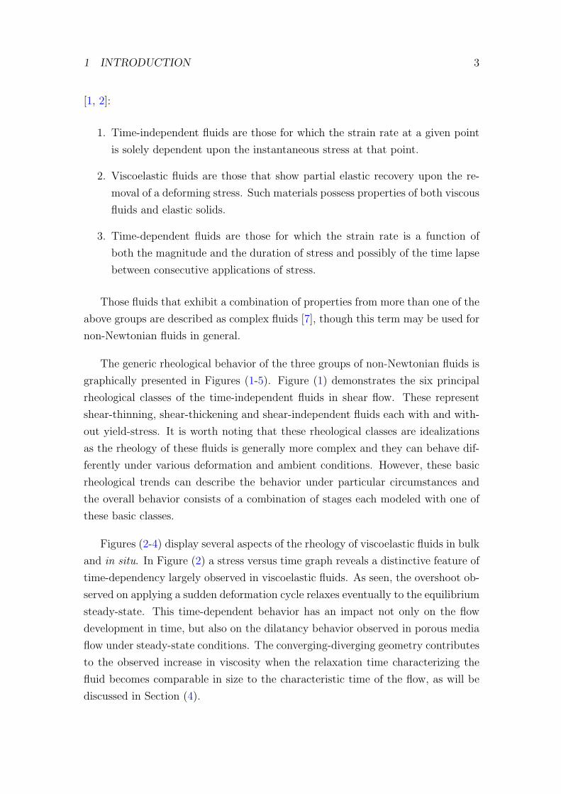
The generic rheological behavior of the three groups of non-Newtonian fluids is

graphically presented in Figures (1-5). Figure (1) demonstrates the six principal

rheological classes of the time-independent fluids in shear flow. These represent

shear-thinning, shear-thickening and shear-independent fluids each with and with-

out yield-stress. It is worth noting that these rheological classes are idealizations

as the rheology of these fluids is generally more complex and they can behave dif-

ferently under various deformation and ambient conditions. However, these basic

rheological trends can describe the behavior under particular circumstances and

the overall behavior consists of a combination of stages each modeled with one of

these basic classes.

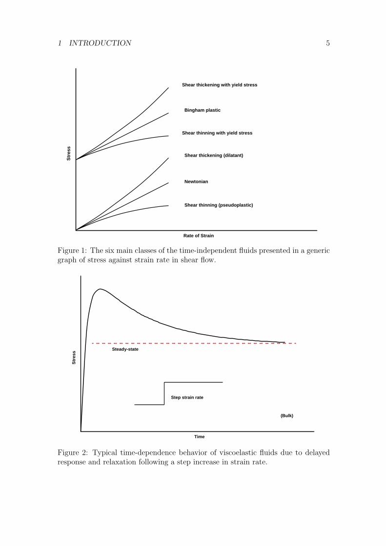
Figures (2-4) display several aspects of the rheology of viscoelastic fluids in bulk

and in situ. In Figure (2) a stress versus time graph reveals a distinctive feature of

time-dependency largely observed in viscoelastic fluids. As seen, the overshoot ob-

served on applying a sudden deformation cycle relaxes eventually to the equilibrium

steady-state. This time-dependent behavior has an impact not only on the flow

development in time, but also on the dilatancy behavior observed in porous media

flow under steady-state conditions. The converging-diverging geometry contributes

to the observed increase in viscosity when the relaxation time characterizing the

fluid becomes comparable in size to the characteristic time of the flow, as will be

discussed in Section (4).

1 INTRODUCTION 4

Figure (3) reveals another characteristic feature of viscoelasticity observed in

porous media flow. The intermediate plateau may be attributed to the time-

dependent nature of the viscoelastic fluid when the relaxation time of the fluid

and the characteristic time of the flow become comparable in size. This behavior

may also be attributed to build-up and break-down due to sudden change in radius

and hence rate of strain on passing through the converging-diverging pores. A

thixotropic nature will be more appropriate in this case.

Figure (4) presents another typical feature of viscoelastic fluids. In addition to

the low-deformation Newtonian plateau and the shear-thinning region which are

widely observed in many time-independent fluids and modeled by various time-

independent rheological models, there is a thickening region which is believed to

be originating from the dominance of extension over shear at high flow rates. This

feature is mainly observed in the flow through porous media, and the converging-

diverging geometry is usually given as an explanation for the shift in dominance

from shear to extension at high flow rates.

In Figure (5) the two basic classes of time-dependent fluids are presented and

compared to the time-independent fluid in a graph of stress versus time of deforma-

tion under constant strain rate condition. As seen, thixotropy is the equivalent in

time to shear-thinning, while rheopexy is the equivalent in time to shear-thickening.

A large number of models have been proposed in the literature to model all types

of non-Newtonian fluids under diverse flow conditions. However, the majority of

these models are basically empirical in nature and arise from curve-fitting exercises

[6]. In the following sections, the three groups of non-Newtonian fluids will be

investigated and a few prominent examples of each group will be presented.

1 INTRODUCTION 5

Rate of Strain

Stre

ss

Shear thickening (dilatant)

Shear thinning (pseudoplastic)

Newtonian

Bingham plastic

Shear thickening with yield stress

Shear thinning with yield stress

Figure 1: The six main classes of the time-independent fluids presented in a genericgraph of stress against strain rate in shear flow.

Time

Stre

ss

Steady-state

Step strain rate

(Bulk)

Figure 2: Typical time-dependence behavior of viscoelastic fluids due to delayedresponse and relaxation following a step increase in strain rate.

1 INTRODUCTION 6

Rate of Strain

Visc

osity

(In situ)

High plateau

Intermediate plateau

Low plateau

Figure 3: Intermediate plateau typical of in situ viscoelastic behavior due to timecharacteristics of the fluid and flow system and converging-diverging nature of theflow channels.

Rate of Strain

Visc

osity

(In situ)

Newtonian Shear-dominated region Extension-dominated region

Figure 4: Strain hardening at high strain rates typical of in situ viscoelastic flowattributed to the dominance of extension over shear at high flow rates.

1.1 Time-Independent Fluids 7

Time

Stre

ss

Rheopectic

Time independent

Thixotropic

Constant strain rate

Figure 5: The two classes of time-dependent fluids compared to the time-independent presented in a generic graph of stress against time.

1.1 Time-Independent Fluids

Shear rate dependence is one of the most important and defining characteristics of

non-Newtonian fluids in general and time-independent fluids in particular. When

a typical non-Newtonian fluid experiences a shear flow the viscosity appears to be

Newtonian at low shear rates. After this initial Newtonian plateau the viscosity is

found to vary with increasing shear rate. The fluid is described as shear-thinning

or pseudoplastic if the viscosity decreases, and shear-thickening or dilatant if the

viscosity increases on increasing shear rate. After this shear-dependent regime,

the viscosity reaches a limiting constant value at high shear rate. This region

is described as the upper Newtonian plateau. If the fluid sustains initial stress

without flowing, it is called a yield-stress fluid. Almost all polymer solutions that

exhibit a shear rate dependent viscosity are shear-thinning, with relatively few

polymer solutions demonstrating dilatant behavior. Moreover, in most known cases

of shear-thickening there is a region of shear-thinning at lower shear rates [3, 5, 6].

In this article, we present four fluid models of the time-independent group:

power-law, Ellis, Carreau and Herschel-Bulkley. These are widely used in modeling

non-Newtonian fluids of this group.

1.1.1 Power-Law Model 8

1.1.1 Power-Law Model

The power-law, or Ostwald-de Waele model, is one of the simplest time-independent

fluid models as it contains only two parameters. The model is given by the relation

[5, 8]

µ = Cγn−1 (3)

where µ is the viscosity, C is the consistency factor, γ is the shear rate and n

is the flow behavior index. In Figure (6), the bulk rheology of this model for

shear-thinning case is presented in a generic form as viscosity versus shear rate

on log-log scales. The power-law is usually used to model shear-thinning though

it can also be used for modeling shear-thickening by making n > 1. The major

weakness of power-law model is the absence of plateaux at low and high shear rates.

Consequently, it fails to produce sensible results in these shear regimes.

Shear Rate

Visc

osity

Slope = n - 1

Figure 6: The bulk rheology of a power-law fluid on logarithmic scales for finiteshear rates (γ > 0).

1.1.2 Ellis Model

This is a three-parameter model that describes time-independent shear-thinning

non-yield-stress fluids. It is used as a substitute for the power-law model and is

1.1.3 Carreau Model 9

appreciably better than the power-law in matching experimental measurements.

Its distinctive feature is the low-shear Newtonian plateau without a high-shear

plateau. According to this model, the fluid viscosity µ is given by [5, 8, 9, 10]

µ =µo

1 +

(τ

τ1/2

)α−1 (4)

where µo is the low-shear viscosity, τ is the shear stress, τ1/2

is the shear stress at

which µ = µo/2 and α is an indicial parameter related to the power-law index by

α = 1/n. A generic graph demonstrating the bulk rheology, that is viscosity versus

shear rate on logarithmic scales, is shown in Figure (7).

Shear Rate

Visc

osity

μο

2

τ = τ1/2

Low-shear plateau

Shear-thinning region

Slope =1 − α

α

μο

Figure 7: The bulk rheology of an Ellis fluid on logarithmic scales for finite shearrates (γ > 0).

1.1.3 Carreau Model

This is a four-parameter rheological model that can describe shear-thinning fluids

with no yield-stress. It is generally praised for its compliance with experiment. The

distinctive feature of this model is the presence of low- and high-shear plateaux.

1.1.4 Herschel-Bulkley Model 10

The Carreau fluid is given by the relation [8]

µ = µ∞ +µo − µ∞

[1 + (γtc)2]1−n

2

(5)

where µ is the fluid viscosity, µ∞ is the viscosity at infinite shear rate, µo is the

viscosity at zero shear rate, γ is the shear rate, tc is a characteristic time and n

is the flow behavior index. A generic graph demonstrating the bulk rheology is

shown in Figure (8).

Shear Rate

Visc

osity

Low-shear plateau

Shear-thinning region

μο

μ∞

Slope = n - 1

High-shear plateau

Figure 8: The bulk rheology of a Carreau fluid on logarithmic scales for finite shearrates (γ > 0).

1.1.4 Herschel-Bulkley Model

The Herschel-Bulkley is a simple rheological model with three parameters. De-

spite its simplicity it can describe the Newtonian and all main classes of the time-

independent non-Newtonian fluids. It is given by the relation [1, 8]

τ = τo + Cγn (τ > τo) (6)

where τ is the shear stress, τo is the yield-stress above which the substance starts

to flow, C is the consistency factor, γ is the shear rate and n is the flow behavior

1.2 Viscoelastic Fluids 11

index. The Herschel-Bulkley model reduces to the power-law when τo = 0, to the

Bingham plastic when n = 1, and to the Newton’s law for viscous fluids when both

these conditions are satisfied.

There are six main classes to this model:

1. Shear-thinning (pseudoplastic) [τo = 0, n < 1]

2. Newtonian [τo = 0, n = 1]

3. Shear-thickening (dilatant) [τo = 0, n > 1]

4. Shear-thinning with yield-stress [τo > 0, n < 1]

5. Bingham plastic [τo > 0, n = 1]

6. Shear-thickening with yield-stress [τo > 0, n > 1]

These classes are graphically illustrated in Figure (1).

1.2 Viscoelastic Fluids

Polymeric fluids often show strong viscoelastic effects. These include shear-thinning,

extension-thickening, normal stresses, and time-dependent rheology. No theory is

yet available that can adequately describe all of the observed viscoelastic phenom-

ena in a variety of flows. Nonetheless, many differential and integral constitutive

models have been proposed in the literature to describe viscoelastic flow. What is

common to all these is the presence of at least one characteristic time parameter

to account for the fluid memory, that is the stress at the present time depends

upon the strain or rate of strain for all past times, but with a fading memory

[3, 11, 12, 13, 14].

Broadly speaking, viscoelasticity is divided into two major fields: linear and

nonlinear. Linear viscoelasticity is the field of rheology devoted to the study of

viscoelastic materials under very small strain or deformation where the displace-

ment gradients are very small and the flow regime can be described by a linear

relationship between stress and rate of strain. In principle, the strain has to be

sufficiently small so that the structure of the material remains unperturbed by the

1.2 Viscoelastic Fluids 12

flow history. If the strain rate is small enough, deviation from linear viscoelastic-

ity may not occur at all. The equations of linear viscoelasticity are not valid for

deformations of arbitrary magnitude and rate because they violate the principle of

frame invariance. The validity of linear viscoelasticity when the small-deformation

condition is satisfied with a large magnitude of rate of strain is still an open ques-

tion, though it is widely accepted that linear viscoelastic constitutive equations

are valid in general for any strain rate as long as the total strain remains small.

Nevertheless, the higher the strain rate the shorter the time at which the critical

strain for departure from linear regime is reached [5, 8, 15].

The linear viscoelastic models have several limitations. For example, they can-

not describe strain rate dependence of viscosity or normal stress phenomena since

these are nonlinear effects. Due to the restriction to infinitesimal deformations,

the linear models may be more appropriate for the description of viscoelastic solids

rather than viscoelastic fluids. Despite the limitations of the linear viscoelastic

models and despite being of less interest to the study of flow where the material

is usually subject to large deformation, they are very important in the study of

viscoelasticity for several reasons [5, 8, 16]:

1. They are used to characterize the behavior of viscoelastic materials at small

deformations.

2. They serve as a motivation and starting point for developing nonlinear models

since the latter are generally extensions to the linears.

3. They are used for analyzing experimental data obtained in small deformation

experiments and for interpreting important viscoelastic phenomena, at least

qualitatively.

Non-linear viscoelasticity is the field of rheology devoted to the study of

viscoelastic materials under large deformation, and hence it is the subject of pri-

mary interest to the study of flow of viscoelastic fluids. Nonlinear viscoelastic

constitutive equations are sufficiently complex that very few flow problems can be

solved analytically. Moreover, there appears to be no differential or integral con-

stitutive equation general enough to explain the observed behavior of polymeric

systems undergoing large deformations but still simple enough to provide a basis

for engineering design procedures [1, 5, 17].

1.2.1 Maxwell Model 13

As the linear viscoelasticity models are not valid for deformations of large mag-

nitude because they do not satisfy the principle of frame invariance, Oldroyd and

others tried to extend these models to nonlinear regimes by developing a set of

frame-invariant constitutive equations. These equations define time derivatives in

frames that deform with the material elements. Examples include rotational, upper

and lower convected time derivatives. The idea of these derivatives is to express

the constitutive equation in real space coordinates rather than local coordinates

and hence fulfilling the Oldroyd’s admissibility criteria for constitutive equations.

These admissibility criteria ensures that the equations are invariant under a change

of coordinate system, value invariant under a change of translational or rotational

motion of the fluid element as it goes through space, and value invariant under a

change of rheological history of neighboring fluid elements [5, 16].

There is a large number of rheological equations proposed for the description

of nonlinear viscoelasticity, as a quick survey to the literature reveals. However,

many of these models are extensions or modifications to others. The two most

popular nonlinear viscoelastic models in differential form are the Upper Convected

Maxwell and the Oldroyd-B models.

In the following sections we present two linear and three nonlinear viscoelastic

models in differential form.

1.2.1 Maxwell Model

This is the first known attempt to obtain a viscoelastic constitutive equation. This

simple linear model, with only one elastic parameter, combines the ideas of viscosity

of fluids and elasticity of solids to arrive at an equation for viscoelastic materials

[5, 18]. Maxwell [19] proposed that fluids with both viscosity and elasticity can be

described, in modern notation, by the relation:

τ + λ1∂τ

∂t= µoγ (7)

where τ is the extra stress tensor, λ1 is the fluid relaxation time, t is time, µo is

the low-shear viscosity and γ is the rate of strain tensor.

1.2.2 Jeffreys Model 14

1.2.2 Jeffreys Model

This is a linear model proposed as an extension to the Maxwell model by including

a time derivative of the strain rate, that is [5, 20]:

τ + λ1∂τ

∂t= µo

(γ + λ2

∂γ

∂t

)(8)

where λ2 is the retardation time that accounts for the corrections of this model and

can be seen as a measure of the time the material needs to respond to deformation.

The Jeffreys model has three constants: a viscous parameter µo, and two elastic

parameters, λ1 and λ2. The model reduces to the linear Maxwell when λ2 = 0, and

to the Newtonian when λ1 = λ2 = 0. As observed by several authors, the Jeffreys

model is one of the most suitable linear models to compare with experiment [21].

1.2.3 Upper Convected Maxwell (UCM) Model

To extend the linear Maxwell model to the nonlinear regime, several time deriva-

tives (e.g. upper convected, lower convected and corotational) have been proposed

to replace the ordinary time derivative in the original model. The most commonly

used of these derivatives in conjunction with the Maxwell model is the upper con-

vected. On purely continuum mechanical grounds there is no reason to prefer one

of these Maxwell equations to the others as they all satisfy frame invariance. The

popularity of the upper convected form is due to its more realistic features [3, 8, 16].

The Upper Convected Maxwell (UCM) is the simplest nonlinear viscoelastic

model and is one of the most popular models in numerical modeling and simulation

of viscoelastic flow. Like its linear counterpart, it is a simple combination of the

Newton’s law for viscous fluids and the derivative of the Hook’s law for elastic

solids. Because of its simplicity, it does not fit the rich variety of viscoelastic effects

that can be observed in complex rheological materials [21]. However, it is largely

used as the basis for other more sophisticated viscoelastic models. It represents,

like the linear Maxwell, purely elastic fluids with shear-independent viscosity, i.e.

Boger fluids [22]. UCM also predicts an elongation viscosity that is three times the

shear viscosity, like Newtonian, which is unrealistic feature for most viscoelastic

fluids. The UCM model is obtained by replacing the partial time derivative in the

differential form of the linear Maxwell with the upper convected time derivative,

1.2.4 Oldroyd-B Model 15

that is

τ + λ1

5τ = µoγ (9)

where τ is the extra stress tensor, λ1 is the relaxation time, µo is the low-shear

viscosity, γ is the rate of strain tensor, and5τ is the upper convected time derivative

of the stress tensor. This time derivative is given by

5τ =

∂τ

∂t+ v · ∇τ − (∇v)T · τ − τ · ∇v (10)

where t is time, v is the fluid velocity, (·)T is the transpose of tensor and ∇v is

the fluid velocity gradient tensor defined by Equation (29) in Appendix 8. The

convected derivative expresses the rate of change as a fluid element moves and

deforms. The first two terms in Equation (10) comprise the material or substantial

derivative of the extra stress tensor. This is the time derivative following a material

element and describes time changes taking place at a particular element of the

‘material’ or ‘substance’. The two other terms in (10) are the deformation terms.

The presence of these terms, which account for convection, rotation and stretching

of the fluid motion, ensures that the principle of frame invariance holds, that is

the relationship between the stress tensor and the deformation history does not

depend on the particular coordinate system used for the description [4, 5, 8].

Despite the simplicity and limitations of the UCM model, it predicts impor-

tant viscoelastic properties such as first normal stress difference in shear and strain

hardening in elongation. It also predicts the existence of stress relaxation after

cessation of flow and elastic recoil. However, according to the UCM the shear vis-

cosity and the first normal stress difference are independent of shear rate and hence

the model fails to describe the behavior of most viscoelastic fluids. Furthermore,

it predicts a steady-state elongational viscosity that becomes infinite at a finite

elongation rate, which is obviously far from physical reality [16].

1.2.4 Oldroyd-B Model

The Oldroyd-B model is a simple form of the more elaborate and rarely used

Oldroyd 8-constant model which also contains the upper convected, the lower con-

vected, and the corotational Maxwell equations as special cases. Oldroyd-B is the

second simplest nonlinear viscoelastic model and is apparently the most popular in

viscoelastic flow modeling and simulation. It is the nonlinear equivalent of the lin-

1.2.5 Bautista-Manero Model 16

ear Jeffreys model, as it takes account of frame invariance in the nonlinear regime.

Oldroyd-B model can be obtained by replacing the partial time derivatives in the

differential form of the Jeffreys model with the upper convected time derivatives

[5]

τ + λ1

5τ = µo

(γ + λ2

5γ

)(11)

where5γ is the upper convected time derivative of the rate of strain tensor given by

5γ =

∂γ

∂t+ v · ∇γ − (∇v)T · γ − γ · ∇v (12)

Oldroyd-B model reduces to the UCM when λ2 = 0, and to Newtonian when

λ1 = λ2 = 0. Despite the simplicity of the Oldroyd-B model, it shows good qualita-

tive agreement with experiments especially for dilute solutions of macromolecules

and Boger fluids. The model is able to describe two of the main features of vis-

coelasticity, namely normal stress difference and stress relaxation. It predicts a

constant viscosity and first normal stress difference with zero second normal stress

difference. Moreover, the Oldroyd-B, like the UCM model, predicts an elongation

viscosity that is three times the shear viscosity, as it is the case in Newtonian fluids.

It also predicts an infinite extensional viscosity at a finite extensional rate, which

is physically unrealistic [3, 5, 15, 21, 23].

A major limitation of the UCM and Oldroyd-B models is that they do not

allow for strain dependency and second normal stress difference. To account for

strain dependent viscosity and non-zero second normal stress difference among

other phenomena, more sophisticated models such as Giesekus and Phan-Thien-

Tanner (PTT) which introduce additional parameters should be considered. Such

equations, however, have rarely been used because of the theoretical and experi-

mental complications they introduce [24].

1.2.5 Bautista-Manero Model

This model combines the Oldroyd-B constitutive equation for viscoelasticity (11)

and the Fredrickson’s kinetic equation for flow-induced structural changes which

may by associated with thixotropy. The model requires six parameters that have

physical significance and can be estimated from rheological measurements. These

parameters are the low and high shear rate viscosities, the elastic modulus, the

1.3 Time-Dependent Fluids 17

relaxation time, and two other constants describing the build up and break down

of viscosity.

The kinetic equation of Fredrickson that accounts for the destruction and con-

struction of structure is given by

dµ

dt=µ

λ

(1− µ

µo

)+ kµ

(1− µ

µ∞

)τ : γ (13)

where µ is the viscosity, t is the time of deformation, λ is the relaxation time upon

the cessation of steady flow, µo and µ∞ are the viscosities at zero and infinite shear

rates respectively, k is a parameter that is related to a critical stress value below

which the material exhibits primary creep, τ is the stress tensor and γ is the rate

of strain tensor. In this model λ is a structural relaxation time whereas k is a

kinetic constant for structure break down. The elastic modulus Go is related to

these parameters by Go = µ/λ [25, 26, 27, 28].

The Bautista-Manero model was originally proposed for the rheology of worm-

like micellar solutions which usually have an upper Newtonian plateau and show

strong signs of shear-thinning. The model, which incorporates shear-thinning,

elasticity and thixotropy, can be used to describe the complex rheological be-

havior of viscoelastic systems that also exhibit thixotropy and rheopexy under

shear flow. It predicts stress relaxation, creep, and the presence of thixotropic

loops when the sample is subjected to transient stress cycles. This model can also

match steady shear, oscillatory and transient measurements of viscoelastic solutions

[25, 26, 27, 28].

1.3 Time-Dependent Fluids

It is generally recognized that there are two main types of time-dependent fluids:

thixotropic (work softening) and rheopectic (work hardening or anti-thixotropic)

depending upon whether the stress decreases or increases with time at a given

strain rate and constant temperature. There is also a general consensus that the

time-dependent feature is caused by reversible structural change during the flow

process. However, there are many controversies about the details, and the theory

of time-dependent fluids is not well developed. Many models have been proposed

in the literature to describe the complex rheological behavior of time-dependent

fluids. Here we present only two models of this group.

1.3.1 Godfrey Model 18

1.3.1 Godfrey Model

Godfrey [29] suggested that at a particular shear rate the time dependence of

thixotropic fluids can be described by the relation

µ(t) = µi−∆µ

′(1− e−t/λ

′

)−∆µ′′(1− e−t/λ

′′

) (14)

where µ(t) is the time-dependent viscosity, µi

is the viscosity at the commencement

of deformation, ∆µ′

and ∆µ′′

are the viscosity deficits associated with the decay

time constants λ′

and λ′′

respectively, and t is the time of shearing. The initial

viscosity specifies a maximum value while the viscosity deficits specify the reduction

associated with the particular time constants. As usual, the time constants define

the time scales of the process under examination. Although Godfrey was originally

proposed as a thixotropic model it can be easily extended to include rheopexy.

1.3.2 Stretched Exponential Model

This is a general time-dependent model that can describe both thixotropic and

rheopectic rheologies [30]. It is given by

µ(t) = µi+ (µ

inf− µ

i)(1− e−(t/λs)c

) (15)

where µ(t) is the time-dependent viscosity, µi

is the viscosity at the commencement

of deformation, µinf

is the equilibrium viscosity at infinite time, t is the time of

deformation, λs is a time constant and c is a dimensionless constant which in the

simplest case is unity.

2 MODELING THE FLOW OF FLUIDS 19

2 Modeling the Flow of Fluids

The basic equations describing the flow of fluids consist of the basic laws of con-

tinuum mechanics which are the conservation principles of mass, energy and linear

and angular momentum. These governing equations indicate how the mass, energy

and momentum of the fluid change with position and time. The basic equations

have to be supplemented by a suitable rheological equation of state, or constitutive

equation describing a particular fluid, which is a differential or integral mathemat-

ical relationship that relates the extra stress tensor to the rate of strain tensor in

general flow condition and closes the set of governing equations. One then solves

the constitutive model together with the conservation laws using a suitable method

to predict the velocity and stress field of the flow [5, 8, 14, 31, 32, 33].

In the case of Navier-Stokes flows the constitutive equation is the Newtonian

stress relation [4] as given in (2). In the case of more rheologically complex flows

other non-Newtonian constitutive equations, such as Ellis and Oldroyd-B, should

be used to bridge the gap and obtain the flow fields. To simplify the situation,

several assumptions are usually made about the flow and the fluid. Common as-

sumptions include laminar, incompressible, steady-state and isothermal flow. The

last assumption, for instance, makes the energy conservation equation redundant.

The constitutive equation should be frame-invariant. Consequently, sophisti-

cated mathematical techniques are employed to satisfy this condition. No single

choice of constitutive equation is best for all purposes. A constitutive equation

should be chosen considering several factors such as the type of flow (shear or

extension, steady or transient, etc.), the important phenomena to capture, the re-

quired level of accuracy, the available computational resources and so on. These

considerations can be influenced strongly by personal preference or bias. Ideally

the rheological equation of state is required to be as simple as possible, involving

the minimum number of variables and parameters, and yet having the capability

to predict the behavior of complex fluids in complex flows. So far, no constitutive

equation has been developed that can adequately describe the behavior of complex

fluids in general flow situation [3, 16]. Moreover, it is very unlikely that such an

equation will be developed in the foreseeable future.

2.1 Modeling Flow in Porous Media 20

2.1 Modeling Flow in Porous Media

In the context of fluid flow, ‘porous medium’ can be defined as a solid matrix

through which small interconnected cavities occupying a measurable fraction of its

volume are distributed. These cavities are of two types: large ones, called pores and

throats, which contribute to the bulk flow of fluid; and small ones, comparable to

the size of the molecules, which do not have an impact on the bulk flow though they

may participate in other transportation phenomena like diffusion. The complexities

of the microscopic pore structure are usually avoided by resorting to macroscopic

physical properties to describe and characterize the porous medium. The macro-

scopic properties are strongly related to the underlying microscopic structure. The

best known examples of these properties are the porosity and the permeability. The

first describes the relative fractional volume of the void space to the total volume

while the second quantifies the capacity of the medium to transmit fluid.

Another important property is the macroscopic homogeneity which may be de-

fined as the absence of local variation in the relevant macroscopic properties, such

as permeability, on a scale comparable to the size of the medium under considera-

tion. Most natural and synthetic porous media have an element of inhomogeneity

as the structure of the porous medium is typically very complex with a degree of

randomness and can seldom be completely uniform. However, as long as the scale

and magnitude of these variations have a negligible impact on the macroscopic

properties under discussion, the medium can still be treated as homogeneous.

The mathematical description of the flow in porous media is extremely complex

and involves many approximations. So far, no analytical fluid mechanics solution to

the flow through porous media has been developed. Furthermore, such a solution is

apparently out of reach in the foreseeable future. Therefore, to investigate the flow

through porous media other methodologies have been developed; the main ones

are the continuum approach, the bundle of tubes approach, numerical methods

and pore-scale network modeling. These approaches are outlined in the following

sections with particular emphasis on the flow of non-Newtonian fluids.

2.1.1 Continuum Models

These widely used models represent a simplified macroscopic approach in which the

porous medium is treated as a continuum. All the complexities and fine details of

2.1.1 Continuum Models 21

the microscopic pore structure are absorbed into bulk terms like permeability that

reflect average properties of the medium. Semi-empirical equations such as Darcy’s

law, Blake-Kozeny-Carman or Ergun equation fall into this category. Commonly

used forms of these equations are given in Table (1). Several continuum models are

based in their derivation on the capillary bundle concept which will be discussed

in the next section.

Darcy’s law in its original form is a linear Newtonian model that relates the

local pressure gradient in the flow direction to the fluid superficial velocity (i.e.

volumetric flow rate per unit cross-sectional area) through the viscosity of the fluid

and the permeability of the medium. Darcy’s law is apparently the simplest model

for describing the flow in porous media, and is widely used for this purpose. Al-

though Darcy’s law is an empirical relation, it can be derived from the capillary

bundle model using Navier-Stokes equation via homogenization (i.e. up-scaling

microscopic laws to a macroscopic scale). Different approaches have been proposed

for the derivation of Darcy’s law from first principles. However, theoretical analysis

reveals that most of these rely basically on the momentum balance equation of the

fluid phase [34]. Darcy’s law is applicable to laminar flow at low Reynolds number

as it contains only viscous term with no inertial term. Typically any flow with a

Reynolds number less than one is laminar. As the velocity increases, the flow en-

ters a nonlinear regime and the inertial effects are no longer negligible. The linear

Darcy’s law may also break down if the flow becomes vanishingly slow as interaction

between the fluid and the pore walls can become important. Darcy flow model also

neglects the boundary effects and heat transfer. In fact the original Darcy model

neglects all effects other than viscous Newtonian effects. Therefore, the validity

of Darcy’s law is restricted to laminar, isothermal, purely viscous, incompress-

ible Newtonian flow. Darcy’s law has been modified differently to accommodate

more complex phenomena such as non-Newtonian and multi-phase flow. Various

generalizations to include nonlinearities like inertia have also been derived using

Table 1: Commonly used forms of the three popular continuum models.

Model Equation

Darcy ∆PL

= µqK

Blake-Kozeny-Carman ∆PL

= 72C′µq(1−ε)2D2

pε3

Ergun ∆PL

= 150µqD2

p

(1−ε)2ε3

+ 1.75ρq2

Dp

(1−ε)ε3


homogenization or volume averaging methods [35].

Blake-Kozeny-Carman (BKC) model for packed bed is one of the most popu-

lar models in the field of fluid dynamics to describe the flow through porous media.

It encompasses a number of equations developed under various conditions and as-

sumptions with obvious common features. This family of equations correlates the

pressure drop across a granular packed bed to the superficial velocity using the fluid

viscosity and the bed porosity and granule diameter. It is also used for modeling

the macroscopic properties of random porous media such as permeability. These

semi-empirical relations are based on the general framework of capillary bundle

with various levels of sophistication. Some forms in this family envisage the bed as

a bundle of straight tubes of complicated cross-section with an average hydraulic

radius. Other forms depict the porous material as a bundle of tortuous tangled

capillary tubes for which the equation of Navier-Stokes is applicable. The effect

of tortuosity on the average velocity in the flow channels gives more accurate por-

trayal of non-Newtonian flow in real beds [36, 37]. The BKC model is valid for

laminar flow through packed beds at low Reynolds number where kinetic energy

losses caused by frequent shifting of flow channels in the bed are negligible. Empiri-

cal extension of this model to encompass transitional and turbulent flow conditions

has been reported in the literature [38].

Ergun equation is a semi-empirical relation that links the pressure drop along

a packed bed to the superficial velocity. It is widely used to portray the flow

through porous materials and to model their physical properties. The input to

the equation is the properties of the fluid (viscosity and mass density) and the bed

(length, porosity and granule diameter). Another, and very popular, form of Ergun

equation correlates the friction factor to the Reynolds number. This form is widely

used for plotting experimental data and may be accused of disguising inaccuracies

and defects. While Darcy and Blake-Kozeny-Carman contain only viscous term,

the Ergun equation contains both viscous and inertial terms. The viscous term is

dominant at low flow rates while the inertial term is dominant at high flow rates

[39, 40]. As a consequence of this duality, Ergun can reach flow regimes that are

not accessible to Darcy or BKC. A proposed derivation of the Ergun equation is

based on a superposition of two asymptotic solutions, one for very low and one for

very high Reynolds number flow. The lower limit, namely the BKC equation, is

quantitatively attributable to a fully developed laminar flow in a three-dimensional


porous structure, while in the higher limit the empirical Burke-Plummer equation

for turbulent flow is applied [41].

The big advantage of the continuum approach is having a closed-form consti-

tutive equation that describes the highly complex phenomenon of flow through

porous media using a few simple compact terms. Consequently, the continuum

models are easy to use with no computational cost. Nonetheless, the continuum

approach suffers from a major limitation by ignoring the physics of flow at pore

level.

Regarding non-Newtonian flow, most of these continuum models have been

employed with some pertinent modification to accommodate non-Newtonian be-

havior. A common approach for single-phase flow is to find a suitable definition

for the effective viscosity which will continue to have the dimensions and phys-

ical significance of Newtonian viscosity [42]. However, many of these attempts,

theoretical and empirical, have enjoyed limited success in predicting the flow of

rheologically-complex fluids in porous media. Limitations of the non-Newtonian

continuum models include failure to incorporate transient time-dependent effects

and to model yield-stress. Some of these issues will be examined in the coming

sections.

The literature of Newtonian and non-Newtonian continuum models is over-

whelming. In the following paragraph we present a limited number of illuminating

examples from the non-Newtonian literature.

Darcy’s law and Ergun’s equation have been used by Sadowski and Bird [9,

43, 44] in their theoretical and experimental investigations to non-Newtonian flow.

They applied the Ellis model to a non-Newtonian fluid flowing through a porous

medium modeled by a bundle of capillaries of varying cross-sections but of a definite

length. This led to a generalized form of Darcy’s law and of Ergun’s friction factor

correlation in each of which the Newtonian viscosity was replaced by an effective

viscosity. A relaxation time term was also introduced as a correction to account

for viscoelastic effects in the case of polymer solutions of high molecular weight.

Gogarty et al [45] developed a modified form of the non-Newtonian Darcy equation

to predict the viscous and elastic pressure drop versus flow rate relationships for

the flow of elastic carboxymethylcellulose (CMC) solutions in beds of different

geometry. Park et al [46, 47] used the Ergun equation to correlate the pressure

2.1.2 Capillary Bundle Models 24

drop to the flow rate for a Herschel-Bulkley fluid flowing through packed beds

by using an effective viscosity calculated from the Herschel-Bulkley model. To

describe the non-steady flow of a yield-stress fluid in porous media, Pascal [48]

modified Darcy’s law by introducing a threshold pressure gradient to account for

yield-stress. This threshold gradient is directly proportional to the yield-stress

and inversely proportional to the square root of the absolute permeability. Al-

Fariss and Pinder [49, 50] produced a general form of Darcy’s law by modifying the

Blake-Kozeny equation to describe the flow in porous media of Herschel-Bulkley

fluids. Chase and Dachavijit [51] modified the Ergun equation to describe the

flow of yield-stress fluids through porous media using the bundle of capillary tubes

approach.

2.1.2 Capillary Bundle Models

In the capillary bundle models the flow channels in a porous medium are depicted

as a bundle of tubes. The simplest form is the model with straight, cylindrical,

identical parallel tubes oriented in a single direction. Darcy’s law combined with

the Poiseuille’s law give the following relationship for the permeability of this model

K =εR2

8(16)

where K and ε are the permeability and porosity of the bundle respectively, and

R is the radius of the tubes.

The advantage of using this simple model, rather than other more sophisticated

models, is its simplicity and clarity. A limitation of the model is its disregard to

the morphology of the pore space and the heterogeneity of the medium. The model

fails to reflect the highly complex structure of the void space in real porous media.

In fact the morphology of even the simplest medium cannot be accurately depicted

by this capillary model as the geometry and topology of real void space have no

similarity to a uniform bundle of tubes. The model also ignores the highly tortuous

character of the flow paths in real porous media with an important impact on the

flow resistance and pressure field. Tortuosity should also have consequences on the

behavior of elastic and yield-stress fluids [36]. Moreover, as it is a unidirectional

model its application is limited to simple one-dimensional flow situations.

One important structural feature of real porous media that is not reflected in


this model is the converging-diverging nature of the pore space which has a sig-

nificant influence on the flow conduct of viscoelastic and yield-stress fluids [52].

Although this simple model may be adequate for modeling some cases of slow flow

of purely viscous fluids through porous media, it does not allow the prediction of

an increase in the pressure drop when used with a viscoelastic constitutive equa-

tion. Presumably, the converging-diverging nature of the flow field gives rise to an

additional pressure drop, in excess to that due to shearing forces, since porous me-

dia flow involves elongational flow components. Therefore, a corrugated capillary

bundle is a better choice for modeling such complex flow fields [42, 53].

Ignoring the converging-diverging nature of flow channels, among other geo-

metrical and topological features, can also be a source of failure for this model

with respect to yield-stress fluids. As a straight bundle of capillaries disregards the

complex morphology of the pore space and because the yield depends on the actual

geometry and connectivity not on the flow conductance, the simple bundle model

will certainly fail to predict the yield point and flow rate of yield-stress fluids in

porous media. An obvious failure of this model is that it predicts a universal yield

point at a particular pressure drop, whereas in real porous media yield is a gradual

process. Furthermore, possible bond aggregation effects due to the connectivity

and size distribution of the flow paths of the porous media are completely ignored

in this model.

Another limitation of this simple model is that the permeability is considered

in the direction of flow only, and hence may not correctly correspond to the perme-

ability of the porous medium especially when it is anisotropic. The model also fails

to consider the pore size distributions. Though this factor may not be of relevance

in some cases where the absolute permeability is of interest, it can be important in

other cases such as yield-stress and certain phenomena associated with two-phase

flow [54].

To remedy the flaws of the uniform bundle of tubes model and to make it more

realistic, several elaborations have been suggested and used; these include

• Using a bundle of capillaries of varying cross-sections. This has been em-

ployed by Sadowski and Bird [9] and other investigators. In fact the model of

corrugated capillaries is widely used especially for modeling viscoelastic flow

in porous media to account for the excess pressure drop near the converging-


diverging regions. The converging-diverging feature may also be used when

modeling the flow of yield-stress fluids in porous media.

• Introducing an empirical tortuosity factor or using a tortuous bundle of cap-

illaries. For instance, in the Blake-Kozeny-Carman model a tortuosity factor

of 25/12 has been used and some forms of the BKC assumes a bundle of

tangled capillaries [36, 55]

• To account for the 3D flow, the model can be improved by orienting 1/3 of

the capillaries in each of the three spatial dimensions. The permeability, as

given by Equation (16), will therefore be reduced by a factor of 3 [54].

• Subjecting the bundle radius size to a statistical distribution that mimics

the size distribution of the real porous media to be modeled by the bundle.

Though we are not aware of such a proposal in the literature, we believe it is

sensible and viable.

It should be remarked that the simple capillary bundle model has been targeted

by heavy criticism. The model certainly suffers from several limitations and flaws

as outlined earlier. However, it is not different to other models and approaches

used in modeling the flow through porous media as they all are approximations

with advantages and disadvantage, limitations and flaws. Like the rest, it can be

an adequate model when applied within its range of validity. Another remark is

that the capillary bundle model is better suited for describing porous media that

are unconsolidated and have high permeability [56]. This seems in line with the

previous remark as the capillary bundle is an appropriate model for this relatively

simple porous medium with comparatively plain structure.

Capillary bundle models have been widely used in the investigation of Newto-

nian and non-Newtonian flow through porous media with various levels of success.

Past experience, however, reveals that no single capillary model can be success-

fully applied in diverse structural and rheological situations. The capillary bundle

should therefore be designed and used with reference to the situation in hand. Be-

cause the capillary bundle models are the basis for most continuum models, as the

latter usually rely in their derivation on some form of capillary models, most of the

previous literature on the use of the continuum approach applies to the capillary

bundle. Here, we give a short list of some contributions in this field in the context

of non-Newtonian flow.

2.1.3 Numerical Methods 27

Sadowski [43, 44] applied the Ellis rheological model to a corrugated capillary

model of a porous medium to derive a modified Darcy’s law. Park [47] used a

capillary model in developing a generalized scale-up method to adapt Darcy’s law

to non-Newtonian fluids. Al-Fariss and Pinder [57] extended the capillary bundle

model to the Herschel-Bulkley fluids and derived a form of the BKC model for

yield-stress fluid flow through porous media at low Reynolds number. Vradis and

Protopapas [58] extended a simple capillary tubes model to describe the flow of

Bingham fluids in porous media and presented a solution in which the flow is zero

below a threshold head gradient and Darcian above it. Chase and Dachavijit [51]

also applied the bundle of capillary tubes approach to model the flow of a yield-

stress fluid through a porous medium, similar to the approach of Al-Fariss and

Pinder.

2.1.3 Numerical Methods

In the numerical approach, a detailed description of the porous medium at pore-

scale with the relevant physics at this level is used. To solve the flow field, numerical

methods, such as finite volume and finite difference, usually in conjunction with

computational implementation are utilized. The advantage of the numerical meth-

ods is that they are the most direct way to describe the physical situation and the

closest to full analytical solution. They are also capable, in principle at least, to

deal with time-dependent transient situations. The disadvantage is that they re-

quire a detailed pore space description. Moreover, they are very complex and hard

to implement with a huge computational cost and serious convergence difficulties.

Due to these complexities, the flow processes and porous media that are currently

within the reach of numerical investigation are the most simple ones. These meth-

ods are also in use for investigating the flow in capillaries with various geometries

as a first step for modeling the flow in porous media and the effect of corrugation

on the flow field.

In the following we present a brief look with some examples from the literature

for using numerical methods to investigate the flow of non-Newtonian fluids in

porous media. In many cases the corrugated capillary was used to model the

converging-diverging nature of the passages in real porous media.

Talwar and Khomami [59] developed a higher order Galerkin finite element

scheme for simulating a two-dimensional viscoelastic flow and tested the algorithm

2.1.4 Pore-Scale Network Modeling 28

on the flow of Upper Convected Maxwell (UCM) and Oldroyd-B fluids in undulating

tube. It was subsequently used to solve the problem of transverse steady flow

of these two fluids past an infinite square arrangement of infinitely long, rigid,

motionless cylinders. Souvaliotis and Beris [60] developed a domain decomposition

spectral collocation method for the solution of steady-state, nonlinear viscoelastic

flow problems. The method was then applied to simulate viscoelastic flows of UCM

and Oldroyd-B fluids through model porous media represented by a square array

of cylinders and a single row of cylinders. Hua and Schieber [61] used a combined

finite element and Brownian dynamics technique (CONNFFESSIT) to predict the

steady-state viscoelastic flow field around an infinite array of squarely-arranged

cylinders using two kinetic theory models. Fadili et al [62] derived an analytical

3D filtration formula for up-scaling isotropic Darcy’s flows of power-law fluids to

heterogeneous Darcy’s flows by using stochastic homogenization techniques. They

then validated their formula by making a comparison with numerical experiments

for 2D flows through a rectangular porous medium using finite volume method.

Concerning the non-uniformity of flow channels and its impact on the flow which

is an issue related to the flow through porous media, numerical techniques have

been used by a number of researchers to investigate the flow of viscoelastic fluids

in converging-diverging geometries. For example, Deiber and Schowalter [11, 63]

used the numerical technique of geometric iteration to solve the nonlinear equations

of motion for viscoelastic flow through tubes with sinusoidal axial variations in

diameter. Pilitsis et al [64] carried a numerical simulation to the flow of a shear-

thinning viscoelastic fluid through a periodically constricted tube using a variety

of constitutive rheological models. Momeni-Masuleh and Phillips [65] used spectral

methods to investigate viscoelastic flow in an undulating tube.

2.1.4 Pore-Scale Network Modeling

The field of network modeling is too diverse and complex to be fairly presented in

this article. We therefore present a general background on this subject followed by

a rather detailed account of one of the network models as an example. This is the

model developed by Blunt and co-workers [66, 67, 68]. One reason for choosing

this example is because it is a well developed model that incorporates the main

features of network modeling in its current state. Moreover, it produced some of

the best results in this field when compared to the available theoretical models

and experimental data. Because of the nature of this article, we will focus on the


single-phase non-Newtonian aspects.

Pore-scale network modeling is a relatively novel method that have been devel-

oped to deal with the flow through porous media and other related issues. It can

be seen as a compromise between the two extremes of continuum and numerical

approaches as it partly accounts for the physics of flow and void space structure

at pore level with affordable computational resources. Network modeling can be

used to describe a wide range of properties from capillary pressure characteris-

tics to interfacial area and mass transfer coefficients. The void space is described

as a network of flow channels with idealized geometry. Rules that determine the

transport properties in these channels are incorporated in the network to compute

effective properties on a mesoscopic scale. The appropriate pore-scale physics com-

bined with a representative description of the pore space gives models that can

successfully predict average behavior [69, 70].

Various network modeling methodologies have been developed and used. The

general feature is the representation of the pore space by a network of intercon-

nected ducts (bonds or throats) of regular shape and the use of a simplified form of

the flow equations to describe the flow through the network. A numerical solver is

usually employed to solve a system of simultaneous equations to determine the flow

field. The network can be two-dimensional or three-dimensional with a random or

regular lattice structure such as cubic. The shape of the cylindrical ducts include

circular, square and triangular cross section (possibly with different shape factor)

and may include converging-diverging feature. The network elements may contain,

beside the conducting ducts, nodes (pores) that can have zero or finite volume and

may well serve a function in the flow phenomena or used as junctions to connect

the bonds. The simulated flow can be Newtonian or non-Newtonian, single-phase,

two-phase or even three-phase. The physical properties of the flow and porous

medium that can be obtained from flow simulation include absolute and relative

permeability, formation factor, resistivity index, volumetric flow rate, apparent vis-

cosity, threshold yield pressure and much more. Typical size of the network is a few

millimeters. One reason for this minute size is to reduce the computational cost.

Another reason is that this size is sufficient to represent a homogeneous medium

having an average throat size of the most common porous materials. Up-scaling

the size of a network is a trivial task if larger pore size is required. Moreover,

extending the size of a network model by attaching identical copies of the same

model in any direction or imposing repeated boundary conditions is another simple


task.

The general strategy in network modeling is to use the bulk rheology of the fluid

and the void space description of the porous medium as an input to the model.

The flow simulation in a network starts by modeling the flow in a single capillary.

The flow in a single capillary can be described by the following general relation

Q = G′∆P (17)

where Q is the volumetric flow rate, G′ is the flow conductance and ∆P is the

pressure drop. For a particular capillary and a specific fluid, G′ is given by

G′ = G′(µ) = constant Newtonian fluid

G′ = G′(µ,∆P ) Purely viscous non-Newtonian fluid

G′ = G′(µ,∆P, t) Fluid with memory (18)

For a network of capillaries, a set of equations representing the capillaries and

satisfying mass conservation have to be solved simultaneously to find the pressure

field and other physical quantities. A numerical solver is usually employed in this

process. For a network with n nodes there are n equations in n unknowns. These

unknowns are the pressure values at the nodes. The essence of these equations

is the continuity of flow of incompressible fluid at each node in the absence of

sources and sinks. To find the pressure field, this set of equations have to be solved

subject to the boundary conditions which are the pressures at the inlet and outlet

of the network. This unique solution is ‘consistent’ and ‘stable’ as it is the only

mathematically acceptable solution to the problem, and, assuming the modeling

process and the mathematical technicalities are reliable, should mimic the unique

physical reality of the pressure field in the porous medium.

For Newtonian fluid, a single iteration is needed to solve the pressure field as

the flow conductance is known in advance because the viscosity is constant. For

purely viscous non-Newtonian fluid, the process starts with an initial guess for

the viscosity, as it is unknown and pressure-dependent, followed by solving the

pressure field iteratively and updating the viscosity after each iteration cycle until

convergence is reached. For memory fluids, the dependence on time must be taken

into account when solving the pressure field iteratively. Apparently, there is no

general strategy to deal with this situation. However, for the steady-state flow of


memory fluids of elastic nature a sensible approach is to start with an initial guess

for the flow rate and iterate, considering the effect of the local pressure and viscosity

variation due to converging-diverging geometry, until convergence is achieved. This

approach was presented by Tardy and Anderson [28] and implemented with some

adaptation by Sochi [68].

With regards to modeling the flow in porous media of complex fluids that have

time dependency in a dynamic sense due to thixotropic or elastic nature, there are

three major difficulties

• The difficulty of tracking the fluid elements in the pores and throats and

identifying their deformation history, as the path followed by these elements

is random and can have several unpredictable outcomes.

• The mixing of fluid elements with various deformation history in the individ-

ual pores and throats. As a result, the viscosity is not a well-defined property

of the fluid in the pores and throats.

• The change of viscosity along the streamline since the deformation history is

continually changing over the path of each fluid element.

These complications can be ignored when dealing with cases of steady-state flow.

Some suggestions on network modeling of time-dependent thixotropic flow will be

presented in Section (5).

Despite all these complications, network modeling in its current state is a sim-

plistic approach that models the flow in ideal situations. Most network models rely

on various simplifying assumptions and disregard important physical processes that

have strong influence on the flow. One such simplification is the use of geometri-

cally uniform network elements to represent the flow channels. Viscoelasticity and

yield-stress are among the physical processes that are compromised by this ideal-

ization of void space. Another simplification is the dissociation of the various flow

phenomena. For example, in modeling the flow of yield-stress fluids through porous

media an implicit assumption is usually made that there is no time dependency or

viscoelasticity. This assumption, however, can be reasonable in the case of model-

ing the dominant effect and may be valid in practical situations where other effects

are absent or insignificant. A third simplification is the adoption of no-slip-at-wall

condition. This widely accepted assumption means that the fluid at the boundary


is stagnant relative to the solid boundary. The effect of slip, which includes reduc-

ing shear-related effects and influencing yield-stress behavior, is very important in

certain circumstances and cannot be ignored. However, this assumption is not far

from reality in many other situations. Furthermore, wall roughness, which is the

rule in porous media, usually prevents wall slip or reduces its effect. Other phys-

ical phenomena that can be incorporated in the network models to make it more

realistic include retention (e.g. by adsorption or mechanical trapping) and wall

exclusion. Most current network models do not take account of these phenomena.

The model of Blunt and co-workers [66, 67, 68], which we present here as

an example, uses three-dimensional networks built from a topologically-equivalent

three-dimensional voxel image of the pore space with the pore sizes, shapes and

connectivity reflecting the real medium. Pores and throats are modeled as having

triangular, square or circular cross-section by assigning a shape factor which is

the ratio of the area to the perimeter squared and obtained from the pore space

image. Most of the network elements are not circular. To account for the non-

circularity when calculating the volumetric flow rate analytically or numerically

for a cylindrical capillary, an equivalent radius Req is used

Req =

(8G

π

)1/4

(19)

where the geometric conductance, G, is obtained empirically from numerical simu-

lation. The network can be extracted from voxel images of a real porous material

or from voxel images generated by simulating the geological processes by which the

porous medium was formed. Examples for the latter are the two networks of Statoil

which represent two different porous media: a sand pack and a Berea sandstone.

These networks are constructed by Øren and coworkers [71, 72] and are used by

several researchers in flow simulation studies. Another possibility for generating

a network is by employing computational algorithms based on numeric statistical

data extracted from the porous medium of interest. Other possibilities can also be

found in the literature.

Assuming a laminar, isothermal and incompressible flow at low Reynolds num-

ber, the only equations that require attention are the constitutive equation for the

particular fluid and the conservation of volume as an expression for the conserva-

tion of mass. For Newtonian flow, the pressure field can be solved once and for all.

For non-Newtonian flow, the situation is more complex as it involves non-linearities


and requires iterative techniques. For the simplest case of time-independent fluids,

the strategy is to start with an arbitrary guess. Because initially the pressure drop

in each network element is not known, an iterative method is used. This starts

by assigning an effective viscosity µe to the fluid in each network element. The

effective viscosity is defined as that viscosity which makes Poiseuille’s equation fits

any set of laminar flow conditions for time-independent fluids [1]. By invoking the

conservation of volume for incompressible fluid, the pressure field across the entire

network is solved using a numerical solver [73]. Knowing the pressure drops in the

network, the effective viscosity of the fluid in each element is updated using the

expression for the flow rate with the Poiseuille’s law as a definition. The pressure

field is then recomputed using the updated viscosities and the iteration continues

until convergence is achieved when a specified error tolerance in the total flow rate

between two consecutive iteration cycles is reached. Finally, the total volumetric

flow rate and the apparent viscosity, defined as the viscosity calculated from the

Darcy’s law, are obtained.

For the steady-state flow of viscoelastic fluids, the approach of Tardy and An-

derson [28, 68] was used as outlined below

• The capillaries of the network are modeled with contraction to account for the

effect of converging-diverging geometry on the flow. The reason is that the

effects of fluid memory take place on going through a radius change, as this

change induces a change in strain rate with a consequent viscosity changing

effects. Examples of the converging-diverging geometries are given in Figure

(9).

• Each capillary is discretized in the flow direction and a discretized form of the

flow equations is used assuming a prior knowledge of the stress and viscosity

at the inlet of the network.

• Starting with an initial guess for the flow rate and using iterative technique,

the pressure drop as a function of the flow rate is found for each capillary.

• Finally, the pressure field for the whole network is found iteratively until

convergence is achieved. Once this happens, the flow rate through each cap-

illary in the network can be computed and the total flow rate through the

network is determined by summing and averaging the flow through the inlet

and outlet capillaries.


Figure 9: Examples of corrugated capillaries that can be used to model converging-diverging geometry in porous media.

For yield-stress fluids, total blocking of the elements below their threshold yield

pressure is not allowed because if the pressure have to communicate, the substance

before yield should be considered a fluid with high viscosity. Therefore, to simulate

the state of the fluid before yield the viscosity is set to a very high but finite value

so the flow virtually vanishes. As long as the yield-stress substance is assumed to

be fluid, the pressure field will be solved as for non-yield-stress fluids because the

situation will not change fundamentally by the high viscosity. It is noteworthy that

the assumption of very high but finite zero-stress viscosity for yield-stress fluids is

realistic and supported by experimental evidence. A further condition is imposed

before any element is allowed to yield, that is the element must be part of a non-

blocked path spanning the network from the inlet to the outlet. What necessitates

this condition is that any conducting element should have a source on one side and

a sink on the other, and this will not happen if either or both sides are blocked.

Finally, a brief look at the literature of network modeling of non-Newtonian flow

through porous media will provide better insight into this field and its contribution

to the subject. In their investigation to the flow of shear-thinning fluids in porous

media, Sorbie et al [54, 74] used 2D network models made up of connected arrays of

capillaries to represent the porous medium. The capillaries were placed on a regular

rectangular lattice aligned with the principal direction of flow, with constant bond

lengths and coordination number 4, but the tube radii are picked from a random

distribution. The non-Newtonian flow in each network element was described by


the Carreau model. Coombe et al [75] used a network modeling approach to ana-

lyze the impact of the non-Newtonian flow characteristics of polymers, foams, and

emulsions at three lengths and time scales. They employed a reservoir simulator to

create networks of varying topology in order to study the impact of porous media

structure on rheological behavior. Shah et al [76] used small size 2D networks to

study immiscible displacement in porous media involving power-law fluids. Their

pore network simulations include drainage where a power-law fluid displaces a New-

tonian fluid at a constant flow rate, and the displacement of one power-law fluid by

another with the same power-law index. Tian and Yao [77] used network models of

cylindrical capillaries on a 2D square lattice to study immiscible displacements of

two-phase non-Newtonian fluids in porous media. In this investigation the injected

and the displaced fluids are considered as Newtonian and non-Newtonian Bingham

fluids respectively.

To study the flow of power-law fluids through porous media, Pearson and Tardy

[42] employed a 2D square-grid network of capillaries, where the radius of each

capillary is randomly distributed according to a predefined probability distribu-

tion function. Their investigation included the effect of the rheological and struc-

tural parameters on the non-Newtonian flow behavior. Tsakiroglou [78, 79] and

Tsakiroglou et al [80] used pore network models on 2D square lattices to inves-

tigate various aspects of single- and two-phase flow of non-Newtonian fluids in

porous media. The rheological models which were employed in this investigation

include Meter, power-law and mixed Meter and power-law. Lopez et al [67, 81, 82]

investigated single- and two-phase flow of shear-thinning fluids in porous media us-

ing network modeling. They used morphologically complex 3D networks to model

the porous media, while the shear-thinning rheology was described by Carreau

model. Balhoff and Thompson [83, 84, 85] employed 3D random network models

extracted from computer-generated random sphere packing to investigate the flow

of shear-thinning and yield-stress fluids in packed beds. The power-law, Ellis and

Herschel-Bulkley fluids were used as rheological models. To model non-Newtonian

flow in the throats, they used analytical expressions for a capillary tube with em-

pirical tuning to key parameters to represent the throat geometry and simulate

the fluid dynamics. Perrin et al [86] used network modeling with Carreau rheology

to analyze their experimental findings on the flow of hydrolyzed polyacrylamide

solutions in etched silicon micromodels. The network simulation was performed on

a 2D network model with a range of rectangular channel widths exactly as in the

physical micromodel experiment. Sochi and Blunt [68, 87] used network modeling


to study single-phase non-Newtonian flow in porous media. Their investigation

includes modeling the Ellis and Herschel-Bulkley as time-independent rheological

models and the Bautista-Manero as a viscoelastic model with thixotropic features.

The non-Newtonian phenomena that can be described by these models include

shear-thinning, shear-thickening, yield-stress, thixotropy and viscoelasticity.

Network modeling was also used by several researchers to investigate the gen-

eration and mobilization of foams and yield-stress fluids in porous media. These

include Rossen and Mamun [88] and Chen et al [89, 90, 91].

3 YIELD-STRESS 37

3 Yield-Stress

Yield-stress or viscoplastic fluids are characterized by their ability to sustain shear

stresses, that is a certain amount of stress must be exceeded before the flow initiates.

So an ideal yield-stress fluid is a solid before yield and a fluid after. Accordingly, the

viscosity of the substance changes from an infinite to a finite value. However, the

physical situation indicates that it is more realistic to regard a yield-stress substance

as a fluid whose viscosity as a function of applied stress has a discontinuity as it

drops sharply from a very high value on exceeding a critical stress.

There are many controversies and unsettled issues in the non-Newtonian lit-

erature about yield-stress phenomenon and yield-stress fluids. In fact, even the

concept of a yield-stress has received much recent criticism, with evidence pre-

sented to suggest that most materials weakly yield or creep near zero strain rate.

The supporting argument is that any material will flow provided that one waits

long enough. These conceptual difficulties are backed by practical and experimen-

tal complications. For example, the value of yield-stress for a particular fluid is

difficult to measure consistently and it may vary by more than an order of magni-

tude depending on the measurement technique [5, 8, 23, 92]. Several constitutive

equations to describe liquids with yield-stress are in use; the most popular ones are

Bingham, Casson and Herschel-Bulkley. Some have suggested that the yield-stress

values obtained via such models should be considered model parameters and not

real material properties.

There are several difficulties in working with yield-stress fluids and validating

the experimental data. One difficulty is that yield-stress value is usually obtained

by extrapolating a plot of shear stress to zero shear rate [8, 46, 49]. This can result

in a variety of values for yield-stress, depending on the distance from the shear

stress axis experimentally accessible by the instrument used. The vast majority of

yield-stress data reported results from such extrapolations, making most values in

the literature instrument-dependent [8]. Another method used to measure yield-

stress is by lowering the shear rate until the shear stress approaches a constant.

This may be described as the dynamic yield-stress [15]. The results obtained using

such methods may not agree with the static yield-stress measured directly without

disturbing the microstructure during the measurement. The latter seems more

relevant to the flow initiation under gradual increase in pressure gradient as in the

case of flow in porous media. Consequently, the accuracy of the predictions made

3.1 Modeling Yield-Stress in Porous Media 38

using flow simulation models in conjunction with such experimental data is limited.

Another difficulty is that while in the case of pipe flow the yield-stress value

is a property of the fluid, in the case of flow in porous media there are strong

indications that in a number of situations it may depend on both the fluid and the

porous medium itself [58, 93]. One possible explanation is that yield-stress value

may depend on the size and shape of the pore space when the polymer molecules

become comparable in size to the pore. The implicit assumption that yield-stress

value at pore-scale is the same as the value at bulk may not be self evident. This

makes the predictions of the models based on analytical solution to the flow in a

uniformly-shaped tube combined with the bulk rheology less accurate. When the

duct size is small, as it is usually the case in porous media, flow of macromolecule

solutions normally displays deviations from predictions based on corresponding

viscometric data [94]. Moreover, the highly complex shape of flow paths in porous

media must have a strong impact on the actual yield point, and this feature is

lost by modeling these paths with ducts of idealized geometry. Consequently, the

concept of equivalent radius Req, which is used in network modeling, though is

completely appropriate for Newtonian fluids and reasonably appropriate for purely

viscous non-Newtonian fluids with no yield-stress, seems inappropriate for yield-

stress fluids as yield depends on the actual shape of the void space rather than the

equivalent radius and flow conductance.

3.1 Modeling Yield-Stress in Porous Media

In this section we outline the failure of the four approaches for modeling the flow

through porous media in dealing with the flow of yield-stress fluids. It is apparent

that no continuum model can predict the yield point of a yield-stress fluid in

complex porous media. The reason is that these models do not account for the

complex geometry and topology of the void space. As the yield point depends on

the fine details of the pore space structure, no continuum model is expected to

predict the threshold yield pressure (TYP) of yield-stress fluids in porous media.

The continuum models also fail to predict the flow rate, at least at transition

stage where the medium is partly conducting, because according to these models

the medium is either fully blocked or fully flowing whereas in reality the yield of

porous medium is a gradual process.

Regarding the capillary bundle models, the situation is similar to the continuum

3.1 Modeling Yield-Stress in Porous Media 39

models as they predict a single universal yield if a uniform bundle of capillaries

is assumed. Moreover, because all capillary bundle models fail to capture the

topology and geometry of complex porous media they cannot predict the yield

point and describe the flow rate of yield-stress fluids in porous media since yield

is highly dependent on the fine details of the void space. An important aspect

of the geometry of real porous media which strongly affects the yield point and

flow rate of yield-stress fluids is the converging-diverging nature of the flow paths.

This feature is not reflected by the bundle of uniform capillaries models. Another

feature is the connectivity of the flow channels where bond aggregation (i.e. how

the throats are distributed and arranged) strongly affects yield behavior.

Concerning the application of numerical methods to yield-stress fluids in porous

media, very few studies can be found on this subject (e.g. [95]). Moreover, the re-

sults, which are reported only for very simple cases of porous media, cannot be fully

assessed. It seems therefore that network modeling is the only viable candidate for

modeling yield-stress fluids in porous media. However, because the research in this

field is limited, no final conclusion on the merit of this approach can be reached.

Nonetheless, the modest success in modeling yield-stress as experienced by some

investigators (e.g. Balhoff [85] and Sochi [68]) indicates that network modeling

in its current state is not capable of dealing with such a complex phenomenon.

One possible reason is the comparative simplicity of the rheological models, such

as Bingham, used in these investigations. These models can possibly offer a phe-

nomenological description of yield-stress in simple flow situations but are certainly

unable to accommodate the underlying physics at pore level in complex porous

media. Consequently, yield-stress as a model parameter obtained in bulk viscom-

etry may not be appropriate to use in this complex situation. Another reason is

the experimental difficulties associated with yield-stress fluids. This can make the

experimental results subject to complications, such as viscoelasticity and retention,

that may not be accounted for in the network model. A third reason is the relative

simplicity of the current network modeling approach to yield-stress fluids. This is

supported by the fact that better results are usually obtained for non-yield-stress

fluids using the same network modeling techniques. One major limitation of the

current network models with regard to yield-stress fluids is the use of analytical

expressions for cylindrical tubes based on the concept of equivalent radius Req.

This is far from reality where the void space retains highly complex shape and

connectivity. Consequently, the yield condition for cylindrical capillaries becomes

invalid approximation to the yield condition for the intricate flow paths in porous

3.2 Predicting Threshold Yield Pressure (TYP) 40

media.

In summary, yield-stress fluid results are extremely sensitive to how the fluid

is characterized, how the void space is described and how the yield process is

modeled. In the absence of a comprehensive and precise incorporation of all these

factors in the network model, pore-scale modeling of yield-stress fluids in porous

media remains a crude approximation that may not produce quantitatively sensible

predictions. The final conclusion is that yield-stress is a problematic phenomenon,

and hence very modest success has been achieved in this area by any one of the

four modeling approaches.

3.2 Predicting Threshold Yield Pressure (TYP)

Here we discuss the attempts to predict the yield point of a complex porous

medium from the void space description and yield-stress value of an ideal yield-

stress fluid without modeling the flow process. In the literature of yield-stress we

can find two well-developed methods proposed for predicting the yield point of

a morphologically-complex network that depicts a porous medium; these are the

Minimum Threshold Path (MTP) and the percolation theory. In this regard, there

is an implicit assumption that the network is an exact replica of the medium and

the yield-stress value reflects the yield-stress of real fluid so that any failure of

these algorithms can not be attributed to mismatch or any factor other than flaws

in these algorithms. It should be remarked that the validity of these methods can

be tested by experiment.

Predicting the threshold yield pressure of a yield-stress fluid in porous media

in its simplest form may be regarded as a special case of the more general problem

of finding the threshold conducting path in disordered media that consist of ele-

ments with randomly distributed thresholds. This problem was analyzed by Roux

and Hansen [96] in the context of studying the conduction of an electric network

of diodes by considering two different cases, one in which the path is directed (no

backtracking) and one in which it is not. They suggested that the minimum overall

threshold potential difference across the network is akin to a percolation threshold

and investigated its dependence on the lattice size. Kharabaf and Yortsos [97] no-

ticed that a firm connection of the lattice-threshold problem to percolation appears

to be lacking and the relation of the Minimum Threshold Path (MTP) to the min-

imum path of percolation, if it indeed exists, is not self-evident. They presented


a new algorithm, Invasion Percolation with Memory (IPM), for the construction

of the MTP, based on which its properties can be studied. The Invasion Percola-

tion with Memory method was further extended by Chen et al [91] to incorporate

dynamic effects due to viscous friction following the onset of mobilization.

The IPM is an algorithm for finding the inlet-to-outlet path that minimizes the

sum of values of a property assigned to the individual elements of the network,

and hence finding this minimum. For a yield-stress fluid, this reduces to finding

the inlet-to-outlet path that minimizes the yield pressure. The yield pressure of

this path is then taken as the network threshold yield pressure. A detailed de-

scription of this algorithm is given in [68, 97]. Other algorithms that achieve this

minimization process can be found in the literature. However, they all rely on a

similar assumption to that upon which the IPM is based, that is the threshold yield

pressure of a network is the minimum sum of the threshold yield pressures of the

individual elements of all possible paths from the inlet to the outlet.

There are two possibilities for defining yield stress fluids before yield: either

solid-like substances or liquids with very high viscosity. According to the first, the

most sensible way for modeling a presumed pressure gradient inside a medium is to

be a constant, that is the pressure drop across the medium is a linear function of the

spatial coordinate in the flow direction, as any other assumption needs justification.

Whereas in the second case the fluid should be treated like non-yield-stress fluids

and hence the pressure field inside the porous medium should be subject to the

consistency criterion for the pressure field which was introduced earlier. The logic

is that the magnitude of the viscosity should have no effect on the flow conduct as

long as the material is assumed to be fluid.

Several arguments can be presented against the MTP algorithms for predicting

the yield point of a medium or a network. Though certain arguments may be more

obvious for a network with cylindrical ducts, they are valid in general for regular

and irregular geometries of flow channels. Some of these arguments are outlined

below

• The MTP algorithms are based on the assumption that the threshold yield

pressure (TYP) of an ensemble of serially connected bonds is the sum of

their yield pressures. This assumption can be challenged by the fact that

for a non-uniform ensemble (i.e. an ensemble whose elements have different

TYPs) the pressure gradient across the ensemble should reach the threshold


yield gradient of the bottleneck (i.e. the element with the highest TYP) of

the ensemble if yield should occur. Consequently, the TYP of the ensemble

will be higher than the sum of the TYPs of the individual elements. This

argument may be more obvious if yield-stress fluids are regarded as solids

and a linear pressure drop is assumed.

• Assuming the yield-stress substances before yield are fluids with high viscos-

ity, the dynamic aspects of the pressure field are neglected because the aim

of the MTP algorithms is to find a collection of bonds inside the network

with a certain condition based on the intrinsic properties of these elements

irrespective of the pressure field. The reality is that the bonds are part of a

network that is subject to a pressure field, so the pressure across each indi-

vidual element must comply with a dynamically stable pressure configuration

over the whole network. The MTP algorithms rely for justification on a hid-

den assumption that the minimum sum condition is identical or equivalent

to the stable configuration condition, which is not obvious, because it is very

unlikely that a stable configuration will require a pressure drop across each

element of the path of minimum sum that is identical to the threshold yield

pressure of that element. Therefor, it is not clear that the actual path of yield

must coincide, totally or partially, with the path of the MTP algorithms let

alone that the actual value of yield pressure must be predicted by these meth-

ods. To sum up, these algorithms disregard the global pressure field which

can communicate with the internal nodes of the serially connected ensemble

as it is part of a network and not an isolated collection of bonds. It is not

obvious that the condition of these algorithms should agree with the require-

ment of a stable and mathematically consistent pressure filed as defined in

Section (2.1). Such an agreement should be regarded as an extremely unlikely

coincidence.

• The MTP algorithms that allows backtracking have another drawback that

is in some cases the path of minimum sum requires a physically unacceptable

pressure configuration. This may be more obvious if the yield-stress sub-

stances are assumed to be solid before yield though it is still valid with the

fluid assumption.

• The effect of tortuosity is ignored since it is implicitly assumed that the

path of yield is an ensemble of serially-connected and linearly-aligned tubes,

whereas in reality the path is generally tortuous as it is part of a network


and can communicate with the global pressure field through the intermediate

nodes. The effect of tortuosity, which is more obvious for the solid assump-

tion, is a possible increase in the external threshold pressure gradient and a

possible change in the bottleneck.

Concerning the percolation approach, it is tempting to consider the conduct

of yield-stress fluids in porous media as a percolation phenomenon to be analyzed

by the classical percolation theory. However, three reasons, at least, may suggest

otherwise

1. The conventional percolation models can be applied only if the conducting

elements are homogeneous, i.e. it is assumed in these models that the intrinsic

property of all elements in the network are equal. However, this assumption

cannot be justified for most kinds of media where the elements vary in their

conduction and yield properties. Therefore, to apply percolation principles, a

generalization to the conventional percolation theory is needed as suggested

by Selyakov and Kadet [98].

2. The network elements cannot yield independently as a spanning path bridging

the inlet to the outlet is a necessary condition for yield. This contradicts the

percolation theory assumption that the elements conduct independently.

3. The pure percolation approach ignores the dynamic aspects of the pressure

field, that is a stable pressure configuration is a necessary condition which

may not coincide with the simple percolation requirement. The percolation

condition, as required by the classic percolation theory, determines the stage

at which the network starts flowing according to the intrinsic properties of

its elements as an ensemble of conducting bonds regardless of the dynamic

aspects introduced by the external pressure field. This argument is more

obvious if yield-stress substances are regarded as fluids with high viscosity.

In a series of studies on generation and mobilization of foam in porous media,

Rossen et al [88, 99] analyzed the threshold yield pressure using percolation theory

concepts and suggested a simple percolation model. In this model, the percolation

cluster is first found, then the MTP was approximated as a subset of this cluster

that samples those bonds with the smallest individual thresholds [91]. This ap-

proach relies on the validity of applying percolation theory to yield-stress, which is


disputed. Moreover, it is a mere coincidence if the yield path is contained within the

percolation sample. Yield is an on/off process which critically depends on factors

other than smallness of individual thresholds. These factors include the particu-

lar distribution and configuration of these elements, being within a larger network

and hence being able to communicate with the global pressure field, and the dy-

namic aspects of the pressure field and stability requirement. Any approximation,

therefore, has very little meaning in this context.

4 VISCOELASTICITY 45

4 Viscoelasticity

Viscoelastic substances exhibit a dual nature of behavior by showing signs of both

viscous fluids and elastic solids. In its most simple form, viscoelasticity can be

modeled by combining Newton’s law for viscous fluids (stress ∝ rate of strain)

with Hook’s law for elastic solids (stress ∝ strain), as given by the original Maxwell

model and extended by the Convected Maxwell models for the nonlinear viscoelas-

tic fluids. Although this idealization predicts several basic viscoelastic phenomena,

it does so only qualitatively. The behavior of viscoelastic fluids is drastically dif-

ferent from that of Newtonian and inelastic non-Newtonian fluids. This includes

the presence of normal stresses in shear flows, sensitivity to deformation type, and

memory effects such as stress relaxation and time-dependent viscosity. These fea-

tures underlie the observed peculiar viscoelastic phenomena such as rod-climbing

(Weissenberg effect), die swell and open-channel siphon [16]. Most viscoelastic

fluids exhibit shear-thinning and an elongational viscosity that is both strain and

extensional strain rate dependent, in contrast to Newtonian fluids where the elon-

gational viscosity is constant and in proportion to shear viscosity [24].

The behavior of viscoelastic fluids at any time is dependent on their recent

deformation history, that is they possess a fading memory of their past. Indeed

a material that has no memory cannot be elastic, since it has no way of remem-

bering its original shape. Consequently, an ideal viscoelastic fluid should behave

as an elastic solid in sufficiently rapid deformations and as a Newtonian liquid in

sufficiently slow deformations. The justification is that the larger the strain rate,

the more strain is imposed on the sample within the memory span of the fluid

[5, 16, 24]. Many materials are viscoelastic but at different time scales that may

not be reached. Dependent on the time scale of the flow, viscoelastic materials

show mainly viscous or elastic behavior. The particular response of a sample in

a given experiment depends on the time scale of the experiment in relation to a

natural time of the material. Thus, if the experiment is relatively slow, the sample

will appear to be viscous rather than elastic, whereas, if the experiment is relatively

fast, it will appear to be elastic rather than viscous. At intermediate time scales

mixed viscoelastic response is observed. Therefore the concept of a natural time

of a material is important in characterizing the material as viscous or elastic. The

ratio between the material time scale and the time scale of the flow is indicated by

a non-dimensional number: the Deborah or the Weissenberg number [6].

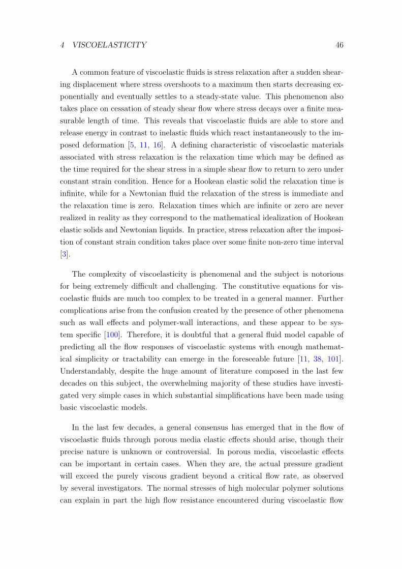
4 VISCOELASTICITY 46

A common feature of viscoelastic fluids is stress relaxation after a sudden shear-

ing displacement where stress overshoots to a maximum then starts decreasing ex-

ponentially and eventually settles to a steady-state value. This phenomenon also

takes place on cessation of steady shear flow where stress decays over a finite mea-

surable length of time. This reveals that viscoelastic fluids are able to store and

release energy in contrast to inelastic fluids which react instantaneously to the im-

posed deformation [5, 11, 16]. A defining characteristic of viscoelastic materials

associated with stress relaxation is the relaxation time which may be defined as

the time required for the shear stress in a simple shear flow to return to zero under

constant strain condition. Hence for a Hookean elastic solid the relaxation time is

infinite, while for a Newtonian fluid the relaxation of the stress is immediate and

the relaxation time is zero. Relaxation times which are infinite or zero are never

realized in reality as they correspond to the mathematical idealization of Hookean

elastic solids and Newtonian liquids. In practice, stress relaxation after the imposi-

tion of constant strain condition takes place over some finite non-zero time interval

[3].

The complexity of viscoelasticity is phenomenal and the subject is notorious

for being extremely difficult and challenging. The constitutive equations for vis-

coelastic fluids are much too complex to be treated in a general manner. Further

complications arise from the confusion created by the presence of other phenomena

such as wall effects and polymer-wall interactions, and these appear to be sys-

tem specific [100]. Therefore, it is doubtful that a general fluid model capable of

predicting all the flow responses of viscoelastic systems with enough mathemat-

ical simplicity or tractability can emerge in the foreseeable future [11, 38, 101].

Understandably, despite the huge amount of literature composed in the last few

decades on this subject, the overwhelming majority of these studies have investi-

gated very simple cases in which substantial simplifications have been made using

basic viscoelastic models.

In the last few decades, a general consensus has emerged that in the flow of

viscoelastic fluids through porous media elastic effects should arise, though their

precise nature is unknown or controversial. In porous media, viscoelastic effects

can be important in certain cases. When they are, the actual pressure gradient

will exceed the purely viscous gradient beyond a critical flow rate, as observed

by several investigators. The normal stresses of high molecular polymer solutions

can explain in part the high flow resistance encountered during viscoelastic flow

4.1 Important Aspects for Flow in Porous Media 47

through porous media. It is believed that the very high normal stress differences

and Trouton ratios associated with polymeric fluids will produce increasing values

of apparent viscosity when the flow channels in the porous medium are of rapidly

changing cross section.

Important aspects of non-Newtonian flow in general and viscoelastic flow in

particular through porous media are still presenting serious challenge for modeling

and quantification. There are intrinsic difficulties in characterizing non-Newtonian

effects in the flow of polymer solutions and the complexities of the local geome-

try of the porous medium. This geometry gives rise to a complex and pore space

dependent flow field in which shear and extension coexist in various proportions

that cannot be quantified. Flows through porous media cannot be classified as

pure shear flows as the converging-diverging passages impose a predominantly ex-

tensional flow fields especially at high flow rates. The extension viscosity of many

non-Newtonian fluids also increases dramatically with the extension rate. As a

consequence, the relationship between the pressure drop and flow rate very often

do not follow the observed Newtonian and inelastic non-Newtonian trend. Further

complications arise from the fact that for complex fluids the stress depends not

only on whether the flow is a shearing, extensional, or mixed type, but also on the

whole history of the velocity gradient [15, 42, 102, 103, 104, 105].

4.1 Important Aspects for Flow in Porous Media

Strong experimental evidence indicates that the flow of viscoelastic fluids through

packed beds can exhibit rapid increases in the pressure drop, or an increase in

the apparent viscosity, above that expected for a comparable purely viscous fluid.

This increase has been attributed to the extensional nature of the flow field in the

pores caused by the successive expansions and contractions that a fluid element

experiences as it traverses the pore space. Although the flow field at pore level is

not an ideal extensional flow due to the presence of shear and rotation, the increase

in flow resistance is referred to as an extension-thickening effect [53, 63, 105, 106]. In

this regard, two major interrelated aspects have strong impact on the flow through

porous media. These are extensional flow and converging-diverging geometry.

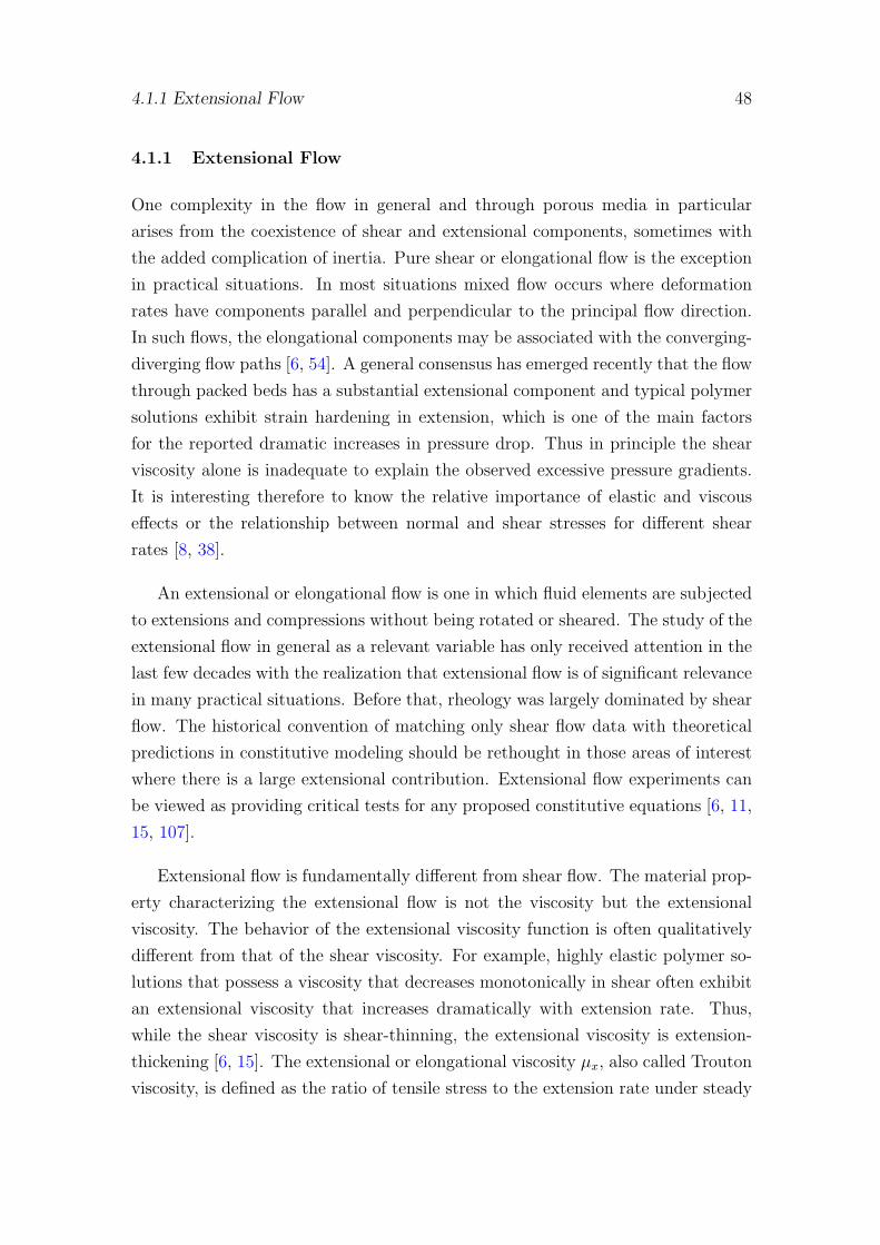
4.1.1 Extensional Flow 48

4.1.1 Extensional Flow

One complexity in the flow in general and through porous media in particular

arises from the coexistence of shear and extensional components, sometimes with

the added complication of inertia. Pure shear or elongational flow is the exception

in practical situations. In most situations mixed flow occurs where deformation

rates have components parallel and perpendicular to the principal flow direction.

In such flows, the elongational components may be associated with the converging-

diverging flow paths [6, 54]. A general consensus has emerged recently that the flow

through packed beds has a substantial extensional component and typical polymer

solutions exhibit strain hardening in extension, which is one of the main factors

for the reported dramatic increases in pressure drop. Thus in principle the shear

viscosity alone is inadequate to explain the observed excessive pressure gradients.

It is interesting therefore to know the relative importance of elastic and viscous

effects or the relationship between normal and shear stresses for different shear

rates [8, 38].

An extensional or elongational flow is one in which fluid elements are subjected

to extensions and compressions without being rotated or sheared. The study of the

extensional flow in general as a relevant variable has only received attention in the

last few decades with the realization that extensional flow is of significant relevance

in many practical situations. Before that, rheology was largely dominated by shear

flow. The historical convention of matching only shear flow data with theoretical

predictions in constitutive modeling should be rethought in those areas of interest

where there is a large extensional contribution. Extensional flow experiments can

be viewed as providing critical tests for any proposed constitutive equations [6, 11,

15, 107].

Extensional flow is fundamentally different from shear flow. The material prop-

erty characterizing the extensional flow is not the viscosity but the extensional

viscosity. The behavior of the extensional viscosity function is often qualitatively

different from that of the shear viscosity. For example, highly elastic polymer so-

lutions that possess a viscosity that decreases monotonically in shear often exhibit

an extensional viscosity that increases dramatically with extension rate. Thus,

while the shear viscosity is shear-thinning, the extensional viscosity is extension-

thickening [6, 15]. The extensional or elongational viscosity µx, also called Trouton

viscosity, is defined as the ratio of tensile stress to the extension rate under steady


flow condition where both these quantities attain constant values. Mathematically,

it is given by

µx =τEε

(20)

where τE (= τ11−τ22) is the normal stress difference and ε is the extension rate. The

stress τ11 is in the direction of the extension while τ22 is in a direction perpendicular

to the extension [6, 108].

Polymeric fluids show a non-constant extensional viscosity in steady and un-

steady extensional flow. In general, extensional viscosity is a function of the ex-

tensional strain rate, just as the shear viscosity is a function of shear rate. It is far

more difficult to measure the extensional viscosity than the shear viscosity. There

is therefore a gulf between the strong desire to measure extensional viscosity and

the likely expectation of its fulfilment [6, 16]. A major difficulty that hinders the

progress in this field is that it is difficult to achieve steady elongational flow and

quantify it precisely. Despite the fact that many techniques have been developed

for measuring the elongational flow properties, these techniques failed so far to

produce consistent outcome as they generate results which can differ by several or-

ders of magnitude. This indicates that these results are dependent on the method

and instrument of measurement. This is highlighted by the view that the exten-

sional viscometers provide measurements of an extensional viscosity rather than

the extensional viscosity. The situation is made more complex by the fact that it

is almost impossible to generate a pure extensional flow since a shear component is

always present in real flow situations, and this makes the measurements doubtful

and inconclusive [2, 5, 6, 8, 15, 104].

For Newtonian and inelastic non-Newtonian fluids the extensional viscosity is a

constant that only depends on the type of extensional deformation. Moreover, the

viscosity measured in a shear flow can be used to predict the viscosity in other types

of deformation. For example, in a simple uniaxial extensional flow of a Newtonian

fluid the following relationship is satisfied

µx = 3µo (21)

For viscoelastic fluids the flow behavior is more complex and the extensional

viscosity, like the shear viscosity, depends on both the strain rate and the time

following the onset of straining. The rheological behavior of a complex fluid in ex-

tension is often very different from that in shear. Polymers usually have extremely


high extensional viscosities which can be orders of magnitude higher than those

expected on the basis of Newtonian model. Moreover, the extensional viscosities

of elastic polymer solutions can be thousands of times greater than their shear

viscosities. To measure the departure of the ratio of extensional to shear viscosity

from its Newtonian equivalent, the rheologists have introduced what is known as

the Trouton ratio which is usually defined as

Tr =µx(ε)

µs(√

3ε)(22)

For elastic liquids, the Trouton ratio is expected to be always greater than

or equal to 3, with the value 3 only attained at vanishingly small strain rates.

These liquids are known for having very high Trouton ratios that can be as high

as l04. This conduct is expected especially when the fluid combines shear-thinning

with tension-thickening. However, even for the fluids that demonstrate tension-

thinning the associated Trouton ratios usually increase with strain rate and are

still significantly in excess of the inelastic value of three [3, 6, 15, 16, 107, 109].

Figures (10) and (11) compare the shear viscosity to the extensional viscosity at

isothermal condition for a typical viscoelastic fluid at various shear and extension

rates. As seen in Figure (10), the shear viscosity curve can be divided into three

regions. For low-shear rates, compared to the time scale of the fluid, the viscosity is

approximately constant. It then equals the so called zero shear rate viscosity. After

this initial plateau the viscosity rapidly decreases with increasing shear rate, and

this behavior is described as shear-thinning. However, there are some materials for

which the reverse behavior is observed, that is the shear viscosity increases with

shear rate giving rise to shear-thickening. For high shear rates the viscosity often

approximates a constant value again. The constant viscosity extremes at low and

high shear rates are known as the lower and upper Newtonian plateau, respectively

[5, 6, 16].

In Figure (11) the typical behavior of the extensional viscosity, µx, of a vis-

coelastic fluid as a function of extension rate, ε, is depicted. As seen, the exten-

sional viscosity curve can be divided into several regions. At low extension rates

the extensional viscosity maintains a constant value known as the zero extension

rate extensional viscosity. This is usually three times the zero shear rate viscosity,

just as for a Newtonian fluid. For somewhat larger extension rates the exten-


Shear Rate

Sh

ea

rV

isc

os

ity

Figure 10: Typical behavior of shear viscosity µs as a function of shear rate γ inshear flow on log-log scales.

Extension Rate

Exte

nsio

nal V

isco

sity

Figure 11: Typical behavior of extensional viscosity µx as a function of extensionrate ε in extensional flow on log-log scales.

4.1.2 Converging-Diverging Geometry 52

sional viscosity increases with increasing extension rate. Some viscoelastic fluids

behave differently, that is their extensional viscosity decreases on increasing exten-

sion rate in this regime. A fluid for which µx increases with increasing ε is said

to be tension-thickening, whilst if µx decreases with increasing ε it is described as

tension-thinning. For even higher extension rates the extension viscosity reaches

a maximum constant value. If the extension rate is increased once more the ex-

tensional viscosity may decrease again. It should be remarked that two polymeric

liquids that may have essentially the same behavior in shear can show a different

response in extension [3, 5, 6, 15].

4.1.2 Converging-Diverging Geometry

An important aspect that characterizes the flow in porous media and makes it

distinct from bulk is the presence of converging-diverging flow paths. This geo-

metric factor significantly affects the flow and accentuate elastic responses. Several

arguments have been presented in the literature to explain the effect of converging-

diverging geometry on the flow behavior. One argument is that viscoelastic flow in

porous media differs from that of Newtonian flow, primarily because the converging-

diverging nature of flow in porous media gives rise to normal stresses which are

not solely proportional to the local shear rate. A second argument is that any

geometry that involves a diameter change will generate a flow field with elonga-

tional characteristics, and hence the flow field in porous media involves both shear

and elongational components with elastic responses. A third argument suggests

that elastic effects are expected in the flow through porous media because of the

acceleration and deceleration of the fluid in the interstices of the bed upon entering

and leaving individual pores [45, 46, 59].

Despite this diversity, there is a general consensus that in porous media the

converging-diverging nature of the flow paths brings out both the extensional and

shear properties of the fluid. The principal mode of deformation to which a mate-

rial element is subjected as the flow converges into a constriction involves both a

shearing of the material element and a stretching or elongation in the direction of

flow, while in the diverging portion the flow involves both shearing and compres-

sion. The actual channel geometry determines the ratio of shearing to extensional

contributions. In many realistic situations involving viscoelastic flows the exten-

sional contribution is the most important of the two modes. As porous media flow

involves elongational flow components, the coil-stretch phenomenon can also take

4.2 Viscoelastic Effects in Porous Media 53

place.

A consequence of the presence of converging-diverging feature in porous media

on flow modeling is that a suitable model pore geometry is one having converging

and diverging sections which can reproduce the elongational nature of the flow.

Despite the general success of the straight capillary tube model with Newtonian

and inelastic non-Newtonian flows, its failure with elastic flow is remarkable. To

rectify the flaws of this model, the undulating tube and converging-diverging chan-

nel were proposed in order to include the elastic character of the flow. Various

corrugated tube models with different simple geometries have been used as a first

step to model the effect of converging-diverging geometry on the flow of viscoelas-

tic fluids in porous media (e.g. [63, 102, 110]). Those geometries include conically

shaped sections, sinusoidal corrugation and abrupt expansions and contractions.

Some simplified forms of these geometries are displayed in Figure (9). Similarly, a

bundle of converging-diverging tubes forms a better model for a porous medium in

viscoelastic flow than the bundle of straight capillary tubes, as the presence of di-

ameter variations makes it possible to account for elongational contributions. Many

investigators have attempted to capture the role of successive converging-diverging

character of packed bed flow by numerically solving the flow equations in conduits

of periodically varying cross sections. Some of these are [11, 38, 53, 59, 111]. Dif-

ferent opinions on the success of these models can be found in the literature. With

regards to modeling viscoelastic flow in regular or random networks of converging-

diverging capillaries, very little work has been done.

4.2 Viscoelastic Effects in Porous Media

In packed bed flows, the main manifestation of steady-state viscoelastic effects is the

excess pressure drop or dilatancy behavior in different flow regimes above what is

accounted for by shear viscosity of the flowing liquid. Qualitatively, this behavior

was attributed either to memory effects or to extensional flow. However, both

explanations have a place as long as the flow regime is considered. Furthermore,

the geometry of the porous media must be taken into account when considering

elastic responses [38, 45].

There is a general agreement that the flow of viscoelastic fluids in packed beds

results in a greater pressure drop than what can be ascribed to the shear rate de-

pendent viscosity. Fluids that exhibit elasticity deviate from viscous flow above

4.2 Viscoelastic Effects in Porous Media 54

some critical velocity in porous flow. At low flow rates, the pressure drop is deter-

mined largely by shear viscosity, and the viscosity and elasticity are approximately

the same as in bulk. As the flow rate gradually increases, viscoelastic effects begin

to appear in various flow regimes. Consequently, the in situ rheological character-

istics become significantly different from those in bulk as elasticity dramatically

increases showing strong dilatant behavior. Although experimental evidence for

viscoelastic effects is convincing, an equally convincing theoretical analysis is not

available. One general argument is that when the fluid suffers a significant de-

formation in a time comparable to the relaxation time of the fluid, elastic effects

become important [8, 38, 45, 101].

The complexity of viscoelastic flow in porous media is aggravated by the pos-

sible occurrence of other non-elastic phenomena which have similar effects as vis-

coelasticity. These phenomena include adsorption of the polymers on the capillary

walls, mechanical retention and partial pore blockage. All these effects also lead

to pressure drops well in excess to that expected from the shear viscosity levels.

Consequently, the interpretation of many observed effects is controversial. Some

authors may interpret some observations in terms of partial pore blockage whereas

others insist on non-Newtonian effects including viscoelasticity as an explanation.

However, none of these have proved to be completely satisfactory. Moreover, no

one can rule out the possibility of simultaneous occurrence of these elastic and in-

elastic phenomena with further complication and confusion. An interesting fact is

the observation made by several researchers, e.g. Sadowski [44], that reproducible

results can be obtained only in constant flow rate experiments because at constant

pressure drop the velocity kept decreasing. This kind of observation indicates de-

position of polymer on the solid surface by one mechanism or another, and cast

doubt on some explanations which involve elasticity. At constant flow rate the in-

creased pressure drop seems to provide the necessary force to keep a reproducible

portion of the flow channels open [10, 38, 103, 112].

There are three principal viscoelastic effects that have to be accounted for in

the investigation of viscoelasticity: transient time-dependence, steady-state time-

dependence and dilatancy at high flow rates.

4.2.1 Transient Time-Dependence 55

4.2.1 Transient Time-Dependence

Transient time-dependent viscoelastic behavior has been observed in bulk on the

startup and cessation of processes involving the displacement of viscoelastic mate-

rials, and on a sudden change of rate or reversal in the direction of deformation.

During these transient states, there are frequently overshoots and undershoots in

stress as a function of time which scale with strain. However, if the fluid is strained

at a constant rate, these transients die out in the course of time, and the stress

approaches a steady-state value that depends only on the strain rate. Under initial

flow conditions stresses can reach magnitudes which are substantially more impor-

tant than their steady-state values, whereas the relaxation on a sudden cessation

of strain can vary substantially in various circumstances [5, 8, 15, 22, 25].

Transient responses are usually investigated in the context of bulk rheology,

despite the fact that there is no available theory that can predict this behavior

quantitatively. As a consequence of this restraint to bulk, the literature of vis-

coelastic flow in porous media is almost entirely dedicated to the steady-state

situation with hardly any work on the in situ time-dependent viscoelastic flows.

However, transient behavior is expected to occur in similar situations during the

flow through porous media. One reason for this gap is the absence of a proper

theoretical structure and the experimental difficulties associated with these flows

in situ. Another possible reason is that the in situ transient flows may have less

important practical applications.

4.2.2 Steady-State Time-Dependence

By this, we mean the effects that arise in the steady-state flow due to time depen-

dency, as time-dependence characteristics of the viscoelastic material must have an

impact on the steady-state conduct. Indeed, elastic effects do occur in steady-state

flow through porous media because of the time-dependence nature of the flow at

pore level. Depending on the time scale of the flow, viscoelastic materials may show

viscous or elastic behavior. The particular response in a given process depends on

the time scale of the process in relation to a natural time of the material. With

regard to this time scale dependency of viscoelastic flow process at pore level, the

fluid relaxation time and the rate of elongation or contraction that occurs as the

fluid flows through a channel or pore with varying cross sectional area should be

used to characterize and quantify viscoelastic behavior [6, 45, 102, 113].

4.2.2 Steady-State Time-Dependence 56

Sadowski and Bird [9] analyzed the viscometric flow problem in a long straight

circular tube and argued that in such a flow no time-dependent elastic effects

are expected. However, in a porous medium elastic effects may occur. As the

fluid moves through a tortuous channel in the porous medium, it encounters a

capriciously changing cross-section. If the fluid relaxation time is small with respect

to the transit time through a contraction or expansion in a tortuous channel, the

fluid will readjust to the changing flow conditions and no elastic effects would be

observed. If, on the other hand, the fluid relaxation time is large with respect to the

time to go through a contraction or expansion, then the fluid will not accommodate

and elastic effects will be observed in the form of an extra pressure drop or an

increase in the apparent viscosity. Thus the concept of a ratio of characteristic

times emerges as an ordering parameter in viscoelastic flow through porous media.

This indicates the importance of the ratio of the natural time of a fluid to the

duration time of a process [10]. It is noteworthy that this formulation relies on

a twofold ordering scheme and is valid for some systems and flow regimes. More

elaborate formulation will be given in conjunction with the intermediate plateau

phenomenon.

One of the steady-state viscoelastic phenomena observed in the flow through

porous media and can be qualified as a time-dependent effect, among other pos-

sibilities such as retention, is the intermediate plateau at medium flow rates as

demonstrated in Figure (3). A possible explanation is that at low flow rates before

the appearance of the intermediate plateau the fluid behaves inelastically like any

typical shear-thinning fluid. This implies that in the low flow regime viscoelastic

effects are negligible as the fluid can respond to the local state of deformation al-

most instantly, that is it does not remember its past and hence behaves as a purely

viscous fluid. As the flow rate increases, a point will be reached where the solid-like

characteristics of viscoelastic materials begin to appear in the form of an increased

apparent viscosity as the time of process becomes comparable to the natural time

of fluid, and hence a plateau is observed. At higher flow rates the process time is

short compared to the natural time of the fluid and hence the fluid has no time

to react as the fluid is not an ideal elastic solid that reacts instantaneously. Since

the process time is very short, no overshoot will occur at the tube constriction as

a measurable finite time is needed for the overshoot to take place. The result is

that no increase in the pressure drop will be observed in this flow regime and the

normal shear-thinning behavior is resumed with the eventual high flow rate plateau

[102, 114].

4.2.3 Dilatancy at High Flow Rates 57

It is noteworthy that Dauben and Menzie [103] have discussed a similar issue in

conjunction with the effect of diverging-converging geometry on the flow through

porous media. They argued that the process of expansion and contraction repeated

many times may account in part for the high pressure drops encountered during

viscoelastic flow in porous media. The fluid relaxation time combined with the

flow velocity determines the response of the viscoelastic fluid in the suggested

diverging-converging model. Accordingly, it is possible that if the relaxation time

is long enough or the fluid velocity high enough the fluid can pass through the

large opening before it has had time to respond to a stress change imposed at the

opening entrance, and hence the fluid would behave more as a viscous and less like

a viscoelastic.

4.2.3 Dilatancy at High Flow Rates

The third distinctive feature of viscoelastic flow is the dilatant behavior in the

form of excess pressure losses at high flow rates as depicted in Figure (4). Certain

polymeric solutions that exhibit shear-thinning in a viscometric flow seem to ex-

hibit a shear-thickening response under appropriate conditions during flow through

porous media. At high flow rates, abnormal increases in flow resistance that resem-

ble a shear-thickening response have been observed in flow experiments involving

a variety of dilute to moderately concentrated solutions of high molecular weight

polymers [10, 54]. This phenomenon can be attributed to stretch-thickening due

to the dominance of extensional over shear flow. At high flow rates, strong exten-

sional flow effects do occur and the extensional viscosity rises very steeply with

increasing extension rate. As a result, the non-shear terms become much larger

than the shear terms. For Newtonian fluids, the extensional viscosity is just three

times the shear viscosity. However, for viscoelastic fluids the shear and extensional

viscosities often behave oppositely, that is while the shear viscosity is generally a

decreasing function of the shear rate, the extensional viscosity increases as the ex-

tension rate increases. The consequence is that the pressure drop will be governed

by extension-thickening and the apparent viscosity rises sharply. Other possibili-

ties such as physical retention are less likely to take place at these high flow rates

[104, 115].

Finally, a glimpse on the literature of viscoelastic flow in porous media will

help to clarify the situation and highlight some important contributions in this


field. Sadowski and Bird [9, 43, 44] were the first to include elastic effects in their

rheological model to account for a departure of the experimental data in porous

media from the modified Darcy’s law [10, 54]. Wissler [101] was the first to account

quantitatively for the elongational stresses developed in viscoelastic flow through

porous media [59]. In this context, he presented a third order perturbation analysis

of a viscoelastic fluid flow through a converging-diverging channel. Gogarty et al

[45] developed a modified form of the non-Newtonian Darcy equation to predict the

viscous and elastic pressure drop versus flow rate relationships for the flow of elastic

carboxymethylcellulose (CMC) solutions in beds of different geometries. Park et

al [46] studied the flow of various polymeric solutions through packed beds using

several rheological models. In the case of one type of solution at high Reynolds

numbers they introduced an empirical corrections based upon a pseudo viscoelastic

Deborah number to improve the data fit.

In their investigation to the flow of polymers through porous media, Hirasaki

and Pope [113] modeled the dilatant behavior by viscoelastic properties of the

polymer solution. The additional viscoelastic resistance to the flow, which is a

function of Deborah number, was modeled as a simple elongational flow to repre-

sent the elongation and contraction that occur as the fluid flows through a pore

with varying cross sectional area. Deiber and Schowalter [11, 63] used a circular

tube with a radius which varies sinusoidally in the axial direction as a first step

toward modeling the flow channels of a porous medium. They concluded that such

a tube exhibits similar phenomenological aspects to those found for the flow of

viscoelastic fluids through packed beds. Durst et al [115] highlighted the fact that

the pressure drop of a porous medium flow is only due to a small extent to the

shear force term usually employed to derive the Kozeny-Darcy law. For a more

correct derivation, additional terms have to be taken into account since the fluid is

also exposed to elongational forces when it passes through the porous media ma-

trix. Chmielewski and coworkers [116, 117, 118] investigated the elastic behavior

of polyisobutylene solutions flowing through arrays of cylinders with various ge-

ometries. They recognized that the converging-diverging geometry of the pores in

porous media causes an extensional flow component that may be associated with

the increased flow resistance for viscoelastic liquids. Pilitsis et al [64] simulated

the flow of a shear-thinning viscoelastic fluid through a periodically constricted

tube using a variety of constitutive rheological models, and the results were com-

pared against the experimental data of Deiber and Schowalter [63]. It was found

that the presence of the elasticity in the mathematical model caused an increase


in the flow resistance over the value calculated for the viscous fluid. Talwar and

Khomami [59] developed a higher order Galerkin finite element scheme for simu-

lating two-dimensional viscoelastic flow and successfully tested the algorithm with

the flow of Upper Convected Maxwell (UCM) and Oldroyd-B fluids in undulating

tube. It was subsequently used to solve the problem of transverse steady flow of

UCM and Oldroyd-B fluids past an infinite square arrangement of infinitely long,

rigid, motionless cylinders.

Garrouch [119] developed a generalized viscoelastic model for polymer flow in

porous media analogous to Darcy’s law, and hence concluded a nonlinear relation-

ship between the fluid velocity and pressure gradient. The model accounts for

polymer elasticity by using the longest relaxation time, and accounts for polymer

viscous properties by using an average porous medium power-law behavior index.

Koshiba et al [120] investigated the viscoelastic flow through an undulating chan-

nel as a model for flow paths in porous media and concluded that the stress in

the flow through the undulating channel should rapidly increase with increasing

flow rate because of the stretch-thickening elongational viscosity. Khuzhayorov

et al [121] applied a homogenization technique to derive a macroscopic filtration

law for describing transient linear viscoelastic fluid flow in porous media. The re-

sults obtained in the particular case of the flow of an Oldroyd fluid in a bundle

of capillary tubes show that viscoelastic behavior strongly differs from Newtonian

behavior. Huifen et al [122] developed a model for the variation of rheological

parameters along the seepage flow direction and constructed a constitutive equa-

tion for viscoelastic fluids in which the variation of the rheological parameters of

polymer solutions in porous media is taken into account. Mendes and Naccache

[104] employed a simple theoretical approach to obtain a constitutive relation for

the flows of extension-thickening fluids through porous media. The pore morphol-

ogy is assumed to be composed of a bundle of periodically converging-diverging

tubes. Dolejs et al [123] presented a method for the pressure drop calculation for

the flow of viscoelastic fluids through fixed beds of particles. The method is based

on the application of the modified Rabinowitsch-Mooney equation together with

the corresponding relations for consistency variables.

5 THIXOTROPY AND RHEOPEXY 60

5 Thixotropy and Rheopexy

Time-dependent fluids are defined to be those fluids whose viscosity depends on the

duration of flow under isothermal conditions. For these fluids, a time-independent

steady-state viscosity is eventually reached in steady flow situation. The time effect

is often reversible though it may be partial, that is the trend of the viscosity change

is overturned in time when the stress is reduced. The phenomenon is generally

attributed to time-dependent thixotropic breakdown or rheopectic buildup of some

particulate structure under relatively high stress followed by structural change in

the opposite direction for lower stress, though the exact mechanism may not be

certain [7, 8, 30, 124, 125].

Time-dependent fluids are generally divided into two main categories: thixotropic

(work softening) whose viscosity gradually decreases with time at a constant shear

rate, and rheopectic (work hardening or anti-thixotropic or negative thixotropic)

whose viscosity increases under similar circumstances without an overshoot which

is a characteristic feature of viscoelasticity. However, it has been proposed that

rheopexy and negative thixotropy are different, and hence three categories of time-

dependent fluids do exist [3, 8, 126]. It is noteworthy that in this article we may

rely on the context and use ‘thixotropy’ conveniently to indicate non-elastic time-

dependence in general where the meaning is obvious.

Thixotropic fluids may be described as shear-thinning while the rheopectic as

shear-thickening, in the sense that these effects take place on shearing, though they

are effects of time-dependence. However, it is proposed that thixotropy invariably

occurs in circumstances where the liquid is shear-thinning (in the usual sense of vis-

cosity decrease with increasing shear rate) while rheopexy may be associated with

shear-thickening. This can be behind the occasional confusion between thixotropy

and shear-thinning [6, 23, 30, 127].

A substantial number of complex fluids display time-dependence phenomena,

with thixotropy being more commonplace and better understood than rheopexy.

Various mathematical models have been proposed to describe time-dependence

behavior. These include microstructural, continuum mechanics, and structural

kinetics models. Thixotropic and rheopectic behaviors may be detected by the

hysteresis loop test, as well as by the more direct steady shear test. In the loop

test the substance is sheared cyclically and a graph of stress versus shear rate


is obtained. A time-dependent fluid should display a hysteresis loop the area of

which is a measure of the degree of thixotropy or rheopexy and this may be used

to quantify time-dependent behavior [2, 7, 125, 126, 127].

In theory, time-dependence effects can arise from thixotropic structural change

or from viscoelasticity. The existence of these two different types of time-dependent

rheologies is generally recognized. Although it is convenient to distinguish between

these as separate types of phenomena, real fluids can exhibit both types of rhe-

ology at the same time. Several physical distinctions between viscoelastic and

thixotropic time-dependence have been made. The important one is that while

the time-dependence of viscoelastic fluids arises because the response of stresses

and strains in the fluid to changes in imposed strains and stresses respectively

is not instantaneous, in thixotropic fluids such response is instantaneous and the

time-dependent behavior arises purely because of changes in the structure of the

fluid as a consequence of strain. While the mathematical theory of viscoelasticity

has been developed to an advanced level, especially on the continuum mechanical

front, relatively little work has been done on thixotropy and rheopexy. One reason

is the lack of a comprehensive framework to describe the dynamics of thixotropy.

This may partly explain why thixotropy is rarely incorporated in the constitu-

tive equation when modeling the flow of non-Newtonian fluids. The underlying

assumption is that in these situations the thixotropic effects have a negligible im-

pact on the resulting flow field, and this allows great mathematical simplifications

[42, 124, 126, 128, 129, 130].

Several behavioral distinctions can be made to differentiate between viscoelas-

ticity and thixotropy. These include the presence or absence of some characteristic

elastic features such as recoil and normal stresses. However, these signs may be of

limited use in some practical situations involving complex fluids where these two

phenomena coexist. In Figure (12) the behavior of these two types of fluids in re-

sponse to step change in strain rate is compared. Although both fluids show signs

of dependency on the past history, the graph suggests that inelastic thixotropic

fluids do not possess a memory in the same sense as viscoelastic materials. The

behavioral differences, such as the absence of elastic effects or the difference in the

characteristic time scale associated with these phenomena, confirm this suggestion

[8, 30, 127, 128].

Thixotropy, like viscoelasticity, is a phenomenon that can appear in a large


Time

Stre

ss

Steady-state

Step strain rate

Thixotropic

Viscoelastic

Figure 12: Comparison between time dependency in thixotropic and viscoelasticfluids following a step increase in strain rate.

number of systems. The time scale for thixotropic changes is measurable in vari-

ous materials including important commercial and biological products. However,

the investigation of thixotropy has been hampered by several difficulties. Conse-

quently, the suggested thixotropic models seem unable to present successful quanti-

tative description of thixotropic behavior especially for the transient state. In fact,

even the most characteristic property of thixotropic fluids, i.e. the decay of vis-

cosity or stress under steady shear conditions, presents difficulties in modeling and

characterization. The lack of a comprehensive theoretical framework to describe

thixotropy is matched by a severe shortage on the experimental side. One reason

is the difficulties confronted in measuring thixotropic systems with sufficient accu-

racy. As a result, very few systematic data sets can be found in the literature and

this deficit hinders the progress in this field. Moreover, the characterization of the

data in the absence of an agreed-upon mathematical structure may be questionable

[29, 124, 125, 127, 128].

5.1 Modeling Time-Dependent Flow in Porous Media 63

5.1 Modeling Time-Dependent Flow in Porous Media

In the absence of serious attempts to model thixotropic rheology in porous media

using the four major modeling approaches (i.e. continuum, capillary bundle, nu-

merical methods and network modeling), very little can be said about this issue. It

seems, however, that network modeling is currently the best candidate for dealing

with this task. In this context, There are three major cases of simulating the flow

of time-dependent fluids in porous media

• The flow of strongly strain-dependent fluid in a porous medium that is not

very homogeneous. This case is very difficult to model because of the difficulty

to track the fluid elements in the pores and throats and determine their

deformation history. Moreover, the viscosity function is not well defined

due to the mixing of fluid elements with various deformation history in the

individual pores and throats.

• The flow of strain-independent or weakly strain-dependent fluid through

porous media in general. A possible strategy is to apply single time-dependent

viscosity function to all pores and throats at each instant of time and hence

simulating time development as a sequence of Newtonian states.

• The flow of strongly strain-dependent fluid in a very homogeneous porous

medium such that the fluid is subject to the same deformation in all network

elements. The strategy for modeling this flow is to define an effective pore

strain rate. Then using a very small time step the strain rate in the next

instant of time can be found assuming constant strain rate. As the change

in the strain rate is now known, a correction to the viscosity due to strain-

dependency can be introduced.

There are two possible problems in this strategy. The first is edge effects

in the case of injection from a reservoir because the deformation history of

the fluid elements at the inlet is different from the deformation history of the

fluid elements inside the network. The second is that considerable computing

resources may be required if very small time steps are used.

The flow of time-dependent fluids in porous media has not been vigorously

investigated. Consequently, very few studies can be found in the literature on this

subject. One reason is that time-dependent effects are usually investigated in the

5.1 Modeling Time-Dependent Flow in Porous Media 64

context of viscoelasticity. Another reason is the lack of a comprehensive framework

to describe the dynamics of time-dependent fluids in porous media [42, 126, 130].

Among the few examples that we found on this subject is the investigation of

Pritchard and Pearson [130] of viscous fingering instability during the injection of

a thixotropic fluid into a porous medium or a narrow fracture. Another example

is the study by Wang et al [131] who examined thixotropic effects in the context

of heavy oil flow through porous media. Finally, some thixotropic aspects were

modeled by Sochi [68] using network modeling approach as part of implementing

the Bautista-Manero rheological model which incorporates thixotropic as well as

viscoelastic effects.

6 EXPERIMENTAL WORK 65

6 Experimental Work on Non-Newtonian Flow

in Porous Media

For completion, we include a brief non-comprehensive list of some experimental

work in the field of non-Newtonian flow through porous media. This collection

should provide a feeling of the nature and topics of experimental research in the

last few decades. The list is arranged in a chronological order

• Sadowski [43, 44] conducted extensive experimental work on the flow of poly-

meric solutions through packed beds. He used ten aqueous polymeric solu-

tions made from Carbowax 20-M, Elvanol 72-51, Natrosol 250G and Natrosol

250H with various concentrations. The porous media were packed beds of lead

shot or glass beads with different properties. He used Ellis as a rheological

model for the fluids and introduced a characteristic time to designate regions

of behavior where elastic effects are important.

• Marshall and Metzner [102] used three polymeric non-Newtonian solutions

(Carbopol 934, polyisobutylene L100 and ET-597) to investigate the flow of

viscoelastic fluids through porous media and determine a Deborah number

at which viscoelastic effects first become measurable. The porous medium

which they used was a sintered bronze porous disk.

• White [132] conducted simple experiments on the flow of a hydroxyethylcel-

lulose solution through a stratified bed using a power-law form of Darcy’s

Law.

• Gogarty et al [45] carried out experiments on the flow of polymer solutions

of carboxymethylcellulose (CMC) and polyacrylamide through three packed

beds of glass beads with various size and a packed bed of sand.

• Park et al [46, 47] experimentally studied the flow of polymeric aqueous solu-

tions of polymethylcellulose (PMC) with different molecular weights and con-

centrations through two packed beds of spherical uniform-in-size glass beads,

coarse and fine. Several rheological models, including Ellis and Herschel-

Bulkley, were used to characterize the fluids.

• Teeuw and Hesselink [133] carried out core flow experiments to investigate

the behavior of aqueous biopolymer solutions in porous media. They used


cylindrical plugs of Bentheim, a clean outcrop sandstone of very uniform

grain size and structure, as porous media characterizing the solutions with

power-law.

• Vogel and Pusch [134] conducted flow experiments on sand pack using three

polymeric solutions: a polysaccharide, a hydroxyethylcellulose and a poly-

acrylamide.

• Al-Fariss and Pinder [49] conducted experimental work on waxy oils modeled

as Herschel-Bulkley fluids. The porous media consist of two packed beds of

sand having different dimensions, porosity, permeability and grain size.

• Durst et al [115] verified aspects of their theoretical non-Newtonian investi-

gation by experimental work on the flow of dilute polymer solutions through

porous media of packed spheres.

• Sorbie et al [135] conducted an extensive experimental and theoretical in-

vestigation on the single-phase flow of Xanthan/tracer slugs in a consoli-

dated sandstone using Carreau rheology. The phenomena studied include

polymer/tracer dispersion, excluded volume effects, polymer adsorption, and

viscous fingering.

• Cannella et al [52] experimentally investigated the flow of Xanthan solutions

through Berea sandstone and carbonate cores in the presence and absence of

residual oil. They used modified power-law and Carreau rheologies in their

theoretical analysis.

• Chmielewski et al [116, 117, 118] conducted experiments to investigate the

elastic behavior of the flow of polyisobutylene solutions through arrays of

cylinders with various geometries.

• Chhabra and Srinivas [136] conducted experimental work investigating the

flow of power-law liquids through beds of non-spherical particles using the

Ergun equation to correlate the resulting values of friction factor. They used

beds of three different types of packing materials (two sizes of Raschig rings

and one size of gravel chips) as porous media and solutions of carboxymethyl-

cellulose as shear-thinning liquids.

• Fletcher et al [137] investigated the flow of biopolymer solutions of Flo-

con 4800MXC, Xanthan CH-100-23, and scleroglucan through Berea and


Clashach cores utilizing Carreau rheological model to characterize the flu-

ids.

• Hejri et al [138] investigated the rheological behavior of biopolymer solutions

of Flocon 4800MX characterized by power-law in sand pack cores.

• Sabiri and Comiti [139] investigated the flow of non-Newtonian purely viscous

fluids through packed beds of spherical particles, long cylinders and very

flat plates. They used aqueous polymeric solutions of carboximethylcellulose

sodium salt. The rheological behavior of these solutions was represented by

a series of power-law type equations.

• Saunders et al [140] carried experimental studies on viscoelastic compression

of resin-impregnated fibre cloths. The experiments included a type of plain-

weave cloth and two types of resin, an epoxy behaving approximately as a

Newtonian fluid and a polyester following power-law non-Newtonian behav-

ior.

• Chase and Dachavijit [51] performed experimental research on aqueous solu-

tions of Carbopol 941 with various concentrations modeled as Bingham fluids.

The porous medium was a packed column of spherical glass beads having a

narrow size distribution.

• Kuzhir et al [141] investigated the flow of a Bingham magneto-rheological

(MR) fluid through different types of porous medium which include bundles

of cylinders and beds of magnetic and non-magnetic spheres.

• D’Angelo et al [142] used radioactive techniques to study the dispersion and

retention phenomena of non-Newtonian scleroglucan polymeric solutions in a

porous medium consisting of an acrylic cylinder filled with compacted glass

microspheres.

• Balhoff and Thompson [84, 85] carried out a limited amount of experimental

work (single dataset) on the flow of guar gum solution in a packed bed of

glass beads. Ellis rheology was used to characterize the fluid.

• Perrin et al [86] conducted experimental work on the flow of hydrolyzed

polyacrylamide (HPAM) solutions in two-dimensional etched silicon wafer

micromodels as idealizations of porous media. The results from these ex-

periments were analyzed by pore-scale network modeling incorporating the

non-Newtonian fluid mechanics of a Carreau fluid.


• Wang et al [131] carried out experimental work on dead oils obtained from

four wells in the Chinese Zaoyuan oilfield by injecting oil into sand pack cores.

The investigation included yield-stress, viscoelastic and thixotropic aspects

using Herschel-Bulkley model.

• Schevena et al [143] conducted experimental research on Newtonian and

non-Newtonian flows through rocks and bead packs. The experiments in-

volved the use of shear-thinning Xanthan solutions and packed beds of near-

monodisperse Ballotini beads.

7 CONCLUSIONS 69

7 Conclusions

In the context of fluid flow, ‘non-Newtonian’ is a generic term that incorporates a

variety of phenomena. These phenomena are highly complex and require sophis-

ticated mathematical modeling techniques for proper description. Further com-

plications are added when considering the flow through porous media. So far no

general methodology that can deal with all cases of non-Newtonian flow has been

developed. Moreover, only modest success has been achieved by any one of these

methodologies. This situation is not expected to change substantially in the fore-

seeable future, and many challenges are still waiting to overcome. In the absence of

a general approach that is suitable for all situations, a combination of all available

approaches is required to tackle non-Newtonian challenges.

Currently, network modeling is the most realistic choice for modeling non-

Newtonian flow in porous media. While this approach is capable of predicting

the general trend in many situations, it is still unable to account for all complexi-

ties and make precise predictions in all cases. The way forward is to improve the

modeling strategies and techniques. One requirement is the improvement of pore

space definition. While modeling the converging-diverging feature of the pore space

with idealized geometry is a step forward, it is not enough. This feature is only

one factor in the making of the complex structure of flow channels. The actual

geometry and topology in porous media is much more complex and should be fully

considered for successful modeling of flow field. Including more physics in the flow

description at pore level is another requirement for reaching the final objective.

8 TERMINOLOGY OF FLOW AND VISCOELASTICITY 70

8 Appendix A

Terminology of Flow and Viscoelasticity∗

A tensor is an array of numbers which transform according to certain rules un-

der coordinate change. In a three-dimensional space, a tensor of order n has 3n

components which may be specified with reference to a given coordinate system.

Accordingly, a scalar is a zero-order tensor and a vector is a first-order tensor.

A stress is defined as a force per unit area. Because both force and area are vec-

tors, considering the orientation of the normal to the area, stress has two directions

associated with it instead of one as with vectors. This indicates that stress should

be represented by a second-order tensor, given in Cartesian coordinate system by

τ =

τxx τxy τxz

τyx τyy τyz

τzx τzy τzz

(23)

where τij is the stress in the j-direction on a surface normal to the i-axis. A shear

stress is a force that a flowing liquid exerts on a surface, per unit area of that

surface, in the direction parallel to the flow. A normal stress is a force per unit

area acting normal or perpendicular to a surface. The components with identical

subscripts represent normal stresses while the others represent shear stresses. Thus

τxx is a normal stress acting in the x-direction on a face normal to x-direction, while

τyx is a shear stress acting in the x-direction on a surface normal to the y-direction,

positive when material at greater y exerts a shear in the positive x-direction on

material at lesser y. Normal stresses are conventionally positive when tensile. The

stress tensor is symmetric that is τij = τji where i and j represent x, y or z. This

symmetry is required by angular momentum considerations to satisfy equilibrium

of moments about the three axes of any fluid element. This means that the state

of stress at a point is determined by six, rather than nine, independent stress

components.

Viscoelastic fluids show normal stress differences in steady shear flows. The

∗In preparing this Appendix, we consulted most of our references. The main ones are [1, 4, 5,6, 15, 16, 22, 144, 145].


first normal stress difference N1 is defined as

N1 = τ11 − τ22 (24)

where τ11 is the normal stress component acting in the direction of flow and τ22 is

the normal stress in the gradient direction. The second normal stress difference N2

is defined as

N2 = τ22 − τ33 (25)

where τ33 is the normal stress component in the indifferent direction. The mag-

nitude of N2 is in general much smaller than N1. For some viscoelastic fluids, N2

may be virtually zero. Often not the first normal stress difference N1 is given, but

a related quantity: the first normal stress coefficient. This coefficient is defined by

Ψ1 = N1

γ2 and decreases with increasing shear rate. Different conventions about the

sign of the normal stress differences do exist. However, in general N1 and N2 show

opposite signs. Viscoelastic solutions with almost the same viscosities may have

very different values of normal stress differences. The presence of normal stress

differences is a strong indication of viscoelasticity, though some associate these

properties with non-viscoelastic fluids.

The total stress tensor, also called Cauchy stress tensor, is usually divided into

two parts: hydrostatic stress tensor and extra stress tensor. The former repre-

sents the hydrostatic pressure while the latter represents the shear and extensional

stresses caused by the flow. In equilibrium the pressure reduces to the hydrostatic

pressure and the extra stress tensor τ vanishes. The extra stress tensor is de-

termined by the deformation history and has to be specified by the constitutive

equation of the particular fluid.

The rate of strain or rate of deformation tensor is a symmetric second order

tensor which gives the components, both extensional and shear, of the strain rate.

In Cartesian coordinate system it is given by:

γ =

γxx γxy γxz

γyx γyy γyz

γzx γzy γzz

(26)

where γxx, γyy and γzz are the extensional components while the others are the


shear components. These components are given by:

γxx = 2∂vx∂x

γyy = 2∂vy∂y

γzz = 2∂vz∂z

γxy = γyx =∂vx∂y

+∂vy∂x

γyz = γzy =∂vy∂z

+∂vz∂y

γxz = γzx =∂vx∂z

+∂vz∂x

(27)

where vx, vy and vz are the velocity components in the respective directions x, y

and z.

The stress tensor is related to the rate of strain tensor by the constitutive or

rheological equation of the fluid which takes a differential or integral form. The

rate of strain tensor γ is related to the fluid velocity vector v, which describes the

steepness of velocity variation as one moves from point to point in any direction in

the flow at a given instant in time, by the relation

γ = ∇v + (∇v)T (28)

where (.)T is the tensor transpose and ∇v is the fluid velocity gradient tensor

defined by

∇v =

∂vx

∂x∂vx

∂y∂vx

∂z∂vy

∂x

∂vy

∂y

∂vy

∂z∂vz

∂x∂vz

∂y∂vz

∂z

(29)

with v = (vx, vy, vz). It should be remarked that the sign and index conventions

used in the definitions of these tensors are not universal.

A fluid possesses viscoelasticity if it is capable of storing elastic energy. A sign

of this is that stresses within the fluid persist after the deformation has ceased.

The duration of time over which appreciable stresses persist after cessation of de-

formation gives an estimate of what is called the relaxation time. The relaxation

and retardation times, λ1 and λ2 respectively, are important physical properties of

viscoelastic fluids because they characterize whether viscoelasticity is likely to be

important within an experimental or observational timescale. They usually have

the physical significance that if the motion is suddenly stopped the stress decays

as e−t/λ1 , and if the stress is removed the rate of strain decays as e−t/λ2 .


For viscous flow, the Reynolds number Re is a dimensionless number defined

as the ratio of the inertial to viscous forces and is given by

Re =ρlcvcµ

(30)

where ρ is the mass density of the fluid, lc is a characteristic length of the flow

system, vc is a characteristic speed of the flow and µ is the viscosity of the fluid.

For viscoelastic fluids the key dimensionless group is the Deborah number which

is a measure of elasticity. This number may be interpreted as the ratio of the

magnitude of the elastic forces to that of the viscous forces. It is defined as the

ratio of a characteristic time of the fluid λc to a characteristic time of the flow

system tc

De =λctc

(31)

The Deborah number is zero for a Newtonian fluid and is infinite for a Hookean elas-

tic solid. High Deborah numbers correspond to elastic behavior and low Deborah

numbers to viscous behavior. As the characteristic times are process-dependent,

materials may not have a single Deborah number associated with them.

Another dimensionless number which measures the elasticity of the fluid is the

Weissenberg number We. It is defined as the product of a characteristic time of

the fluid λc and a characteristic strain rate γc in the flow

We = λcγc (32)

Other definitions to Deborah and Weissenberg numbers are also in common use

and some even do not differentiate between the two numbers. The characteristic

time of the fluid may be taken as the largest time constant describing the molecular

motions, or a time constant in a constitutive equation. The characteristic time for

the flow can be the time interval during which a typical fluid element experiences a

significant sequence of kinematic events or it is taken to be the duration of an ex-

periment or experimental observation. Many variations in defining and quantifying

these characteristics do exit, and this makes Deborah and Weissenberg numbers

not very well defined and measured properties and hence the interpretation of the

experiments in this context may not be totally objective.

The Boger fluids are constant-viscosity non-Newtonian elastic fluids. They


played important role in the recent development of the theory of fluid elasticity as

they allow dissociation between elastic and viscous effects. Boger realized that the

complication of variable viscosity effects can be avoided by employing test liquids

which consist of low concentrations of flexible high molecular weight polymers in

very viscous solvents, and these solutions are nowadays called Boger fluids.

9 NOMENCLATURE 75

9 Appendix B

Nomenclature

α parameter in Ellis model

γ strain

γ rate of strain (s−1)

γc characteristic rate of strain (s−1)

γ rate of strain tensor

ε porosity

ε extension

ε rate of extension (s−1)

λ structural relaxation time in Fredrickson model (s)

λ1 relaxation time (s)

λ2 retardation time (s)

λc characteristic time of fluid (s)

λ′

first time constant in Godfrey model (s)

λ′′

second time constant in Godfrey model (s)

λs time constant in Stretched Exponential Model (s)

µ viscosity (Pa.s)

µe effective viscosity (Pa.s)

µi

initial-time viscosity (Pa.s)

µinf

infinite-time viscosity (Pa.s)

µo zero-shear viscosity (Pa.s)

µs shear viscosity (Pa.s)

µx extensional (elongational) viscosity (Pa.s)

µ∞ infinite-shear viscosity (Pa.s)

∆µ′

viscosity deficit associated with λ′

in Godfrey model (Pa.s)

∆µ′′

viscosity deficit associated with λ′′

in Godfrey model (Pa.s)

ρ fluid mass density (kg.m−3)

τ stress (Pa)

τ stress tensor

τ1/2

stress when µ = µo/2 in Ellis model (Pa)

9 NOMENCLATURE 76

τo yield-stress (Pa)

c dimensionless constant in Stretched Exponential Model

C consistency factor in power-law and Herschel-Bulkley models (Pa.sn)

C ′ tortuosity factor

De Deborah number

Dp particle diameter (m)

G geometric conductance (m4)

G′ flow conductance (m3.Pa−1.s−1)

Go elastic modulus (Pa)

k parameter in Fredrickson model (Pa−1)

K absolute permeability (m2)

L length of tube or bed (m)

lc characteristic length of the flow system (m)

n flow behavior index

N1 first normal stress difference (Pa)

N2 second normal stress difference (Pa)

P pressure (Pa)

∆P pressure drop (Pa)

q superficial (Darcy) velocity (m.s−1)

Q volumetric flow rate (m3.s−1)

R tube radius (m)

Re Reynolds number

Req equivalent radius (m)

t time (s)

tc characteristic time of flow system (s)

Tr Trouton ratio

v fluid velocity vector

∇v fluid velocity gradient tensor

vc characteristic speed of flow system (m.s−1)

We Weissenberg number

Abbreviations:

2D two-dimensional

9 NOMENCLATURE 77

3D three-dimensional

BKC Blake-Kozeny-Carman

IPM Invasion Percolation with Memory

MTP Minimum Threshold Path

TYP Threshold Yield Pressure

(·)T matrix transpose5· upper convected time derivative

Note: units, when relevant, are given in the SI system. Vectors and tensors are

marked with boldface. Some symbols may rely on the context for unambiguous

identification.

REFERENCES 78

References

[1] A.H.P. Skelland. Non-Newtonian Flow and Heat Transfer. John Wiley and

Sons Inc., 1967. 2, 3, 10, 12, 33, 70

[2] R.P. Chhabra; J.F. Richardson. Non-Newtonian Flow in the Process Indus-

tries. Butterworth Heinemann Publishers, 1999. 2, 3, 49, 61

[3] R.G. Owens; T.N. Phillips. Computational Rheology. Imperial College Press,

2002. 2, 7, 11, 14, 16, 19, 46, 50, 52, 60

[4] R.G.M. van Os; T.N. Phillips. Spectral element methods for transient vis-

coelastic flow problems. Journal of Computational Physics, 201(1):286–314,

2004. 2, 15, 19, 70

[5] R.B. Bird; R.C. Armstrong; O. Hassager. Dynamics of Polymeric Liquids,

volume 1. John Wily & Sons, second edition, 1987. 2, 7, 8, 9, 12, 13, 14, 15,

16, 19, 37, 45, 46, 49, 50, 52, 55, 70

[6] H.A. Barnes; J.E Hutton; K. Walters. An introduction to rheology. Elsevier,

1993. 2, 4, 7, 45, 48, 49, 50, 52, 55, 60, 70

[7] A.A. Collyer. Time dependent fluids. Physics Education, 9:38–44, 1974. 3,

60, 61

[8] P.J. Carreau; D. De Kee; R.P. Chhabra. Rheology of Polymeric Systems.

Hanser Publishers, 1997. 8, 9, 10, 12, 14, 15, 19, 37, 48, 49, 54, 55, 60, 61

[9] T.J. Sadowski; R.B. Bird. Non-Newtonian flow through porous media I.

Theoretical. Transactions of the Society of Rheology, 9(2):243–250, 1965. 9,

23, 25, 56, 58

[10] J.G. Savins. Non-Newtonian flow through porous media. Industrial and

Engineering Chemistry, 61(10):18–47, 1969. 9, 54, 56, 57, 58

[11] J.A. Deiber. Modeling the flow of Newtonian and viscoelastic fluids through

porous media. PhD thesis, Princeton University, 1978. 11, 28, 46, 48, 53, 58

[12] M.M. Denn. Issues in viscoelastic fluid mechanics. Annual Review of Fluid

Mechanics, 22:13–34, 1990. 11

REFERENCES 79

[13] M.A. Hulsen. A discontinuous Galerkin method with splitting applied to visco-

elastic flow. Faculty of Mechanical Engineering and Marine Technology, Delft

University of Technology, 1986. 11

[14] R. Keunings. Micro-macro methods for the multi-scale simulation of vis-

coelastic flow using molecular models of kinetic theory. Rheology Reviews,

pages 67–98, 2004. 11, 19

[15] R.G. Larson. The Structure and Rheology of Complex Fluids. Oxford Uni-

versity Press, 1999. 12, 16, 37, 47, 48, 49, 50, 52, 55, 70

[16] R.G. Larson. Constitutive Equations for Polymer Melts and Solutions. But-

terworth Publishers, 1988. 12, 13, 14, 15, 19, 45, 46, 49, 50, 70

[17] J.L. White; A.B. Metzner. Thermodynamic and heat transport consider-

ations for viscoelastic fluids. Chemical Engineering Science, 20:1055–1062,

1965. 12

[18] B. Mena; O. Manero; L.G. Leal. The influence of rheological properties

on the slow flow past spheres. Journal of Non-Newtonian Fluid Mechanics,

26(2):247–275, 1987. 13

[19] J.C. Maxwell. On the dynamical theory of gases. Philosophical Transactions

of the Royal Society of London, 157:49–88, 1867. 13

[20] H. Jeffreys. The Earth Its Origin, History and Physical Constitution. Cam-

bridge University Press, second edition, 1929. 14

[21] J. Martınez-Mardones; C. Perez-Garcıa. Linear instability in viscoelastic fluid

convection. Journal of Physics: Condensed Matter, 2(5):1281–1290, 1990. 14,

16

[22] R.I. Tanner. Engineering Rheology. Oxford University Press, 2nd edition,

2000. 14, 55, 70

[23] N.J. Balmforth; R.V. Craster. Geophysical Aspects of Non-Newtonian Fluid

Mechanics. Springer, 2001. 16, 37, 60

[24] D.V. Boger. Viscoelastic flows through contractions. Annual Review of Fluid

Mechanics, 19:157–182, 1987. 16, 45

REFERENCES 80

[25] F. Bautista; J.M. de Santos; J.E. Puig; O. Manero. Understanding

thixotropic and antithixotropic behavior of viscoelastic micellar solutions and

liquid crystalline dispersions. I. The model. Journal of Non-Newtonian Fluid

Mechanics, 80(2):93–113, 1999. 17, 55

[26] F. Bautista; J.F.A. Soltero; J.H. Perez-Lopez; J.E. Puig; O. Manero. On the

shear banding flow of elongated micellar solutions. Journal of Non-Newtonian

Fluid Mechanics, 94(1):57–66, 2000. 17

[27] O. Manero; F. Bautista; J.F.A. Soltero; J.E. Puig. Dynamics of worm-like

micelles: the Cox-Merz rule. Journal of Non-Newtonian Fluid Mechanics,

106(1):1–15, 2002. 17

[28] P. Tardy; V.J. Anderson. Current modelling of flow through porous media.

Private communication, 2005. 17, 31, 33

[29] J.C. Godfrey. Steady shear measurement of thixotropic fluid properties. Rhe-

ologica Acta, 12(4):540–545, 1973. 18, 62

[30] H.A. Barnes. Thixotropy – a review. Journal of Non-Newtonian Fluid Me-

chanics, 70(1):1–33, 1997. 18, 60, 61

[31] M.A. Hulsen. Analysis of the equations for viscoelastic flow: Type, boundary

conditions, and discontinuities. Faculty of Mechanical Engineering, Delft

University of Technology, 1986. 19

[32] M.A. Hulsen. A numerical method for solving steady 2D and axisymmetrical

viscoelastic flow problems with an application to inertia effects in contraction

flows. Faculty of Mechanical Engineering, Delft University of Technology,

1990. 19

[33] R. Keunings. Finite element methods for integral viscoelastic fluids. Rheology

Reviews, pages 167–195, 2003. 19

[34] W.R. Schowalter. Mechanics of Non-Newtonian Fluids. Pergamon Press Inc.,

1978. 21

[35] A.V. Shenoy. Darcy-Forchheimer natural, forced and mixed convection heat

transfer in non-Newtonian power-law fluid-saturated porous media. Transport

in Porous Media, 11(3):219–241, 1993. 22

REFERENCES 81

[36] W. Kozicki; C. Tiu. A unified model for non-Newtonian flow in packed beds

and porous media. Rheologica Acta, 27(1):31–38, 1988. 22, 24, 26

[37] R.P. Chapuis; M. Aubertin. On the use of the Kozeny-Carman equation to

predict the hydraulic conductivity of soils. Canadian Geotechnical Journal,

40(3):616–628, 2003. 22

[38] R.P. Chhabra; J. Comiti; I. Machac. Flow of non-Newtonian fluids in fixed

and fluidised beds. Chemical Engineering Science, 56(1):1–27, 2001. 22, 46,

48, 53, 54

[39] W.M. Jones. The flow of dilute aqueous solutions of macromolecules in var-

ious geometries: IV. the Ergun and Jones equations for flow through con-

solidated beds. Journal of Physics D: Applied Physics, 9(5):771–772, 1976.

22

[40] P. Stevenson. Comment on “Physical insight into the Ergun and Wen &

Yu equations for fluid flow in packed and fluidised beds”, by R.K. Niven.

Chemical Engineering Science, 58(23):5379–5379, 2003. 22

[41] J.P. Du Plessis. Analytical quantification of coefficients in the Ergun equation

for fluid friction in a packed bed. Transport in Porous Media, 16(2):189–207,

1994. 23

[42] J.R.A. Pearson; P.M.J. Tardy. Models for flow of non-Newtonian and complex

fluids through porous media. Journal of Non-Newtonian Fluid Mechanics,

102(2):447–473, 2002. 23, 25, 35, 47, 61, 64

[43] T.J. Sadowski. Non-Newtonian flow through porous media II. Experimental.

Transactions of the Society of Rheology, 9(2):251–271, 1965. 23, 27, 58, 65

[44] T.J. Sadowski. Non-Newtonian flow through porous media. PhD thesis, Uni-

versity of Wisconsin, 1963. 23, 27, 54, 58, 65

[45] W.B. Gogarty; G.L. Levy; V.G. Fox. Viscoelastic effects in polymer flow

through porous media. SPE 47th Annual Fall Meeting, 8-11 October, San

Antonio, Texas, SPE 4025, 1972. 23, 52, 53, 54, 55, 58, 65

[46] H.C. Park; M.C. Hawley; R.F. Blanks. The flow of non-Newtonian solutions

through packed beds. SPE 4722, 1973. 23, 37, 52, 58, 65

REFERENCES 82

[47] H.C. Park. The flow of non-Newtonian fluids through porous media. PhD

thesis, Michigan State University, 1972. 23, 27, 65

[48] H. Pascal. Nonsteady flow through porous media in the presence of a thresh-

old gradient. Acta Mechanica, 39(3-4):207–224, 1981. 24

[49] T.F. Al-Fariss; K.L. Pinder. Flow of a shear-thinning liquid with yield stress

through porous media. SPE 13840, 1984. 24, 37, 66

[50] T.F. Al-Fariss. A new correlation for non-Newtonian flow through porous

media. Computers and Chemical Engineering, 13(4-5):475–482, 1989. 24

[51] G.G. Chase; P. Dachavijit. Incompressible cake filtration of a yield stress

fluid. Separation Science and Technology, 38(4):745–766, 2003. 24, 27, 67

[52] W.J. Cannella; C. Huh; R.S. Seright. Prediction of Xanthan rheology in

porous media. SPE Annual Technical Conference and Exhibition, 2-5 Octo-

ber, Houston, Texas, SPE 18089, 1988. 25, 66

[53] S. Pilitsis; A.N. Beris. Calculations of steady-state viscoelastic flow in an

undulating tube. Journal of Non-Newtonian Fluid Mechanics, 31(3):231–

287, 1989. 25, 47, 53

[54] K.S. Sorbie. Polymer-Improved Oil Recovery. Blakie and Son Ltd, 1991. 25,

26, 34, 48, 57, 58

[55] J.L. Duda; S. Hang; E.E. Klaus. Flow of polymer solutions in porous media:

Inadequacy of the capillary model. Industrial and Engineering Chemistry

Fundamentals, 22(3):299–305, 1983. 26

[56] A. Zaitoun; N. Kohler. Two-phase flow through porous media: Effect of an

adsorbed polymer layer. SPE Annual Technical Conference and Exhibition,

2-5 October, Houston, Texas, SPE 18085, 1988. 26

[57] T.F. Al-Fariss; K.L. Pinder. Flow through porous media of a shear-

thinning liquid with yield stress. Canadian Journal of Chemical Engineering,

65(3):391–405, 1987. 27

[58] G.C. Vradis; A.L. Protopapas. Macroscopic conductivities for flow of

Bingham plastics in porous media. Journal of Hydraulic Engineering,

119(1):95–108, 1993. 27, 38

REFERENCES 83

[59] K.K. Talwar; B. Khomami. Application of higher order finite element meth-

ods to viscoelastic flow in porous media. Journal of Rheology, 36(7):1377–

1416, 1992. 27, 52, 53, 58, 59

[60] A. Souvaliotis; A.N. Beris. Spectral collocation/domain decomposition

method for viscoelastic flow simulations in model porous geometries. Com-

puter Methods in Applied Mechanics and Engineering, 129(1):9–28, 1996. 28

[61] C.C. Hua; J.D. Schieber. Viscoelastic flow through fibrous media using the

CONNFFESSIT approach. Journal of Rheology, 42(3):477–491, 1998. 28

[62] A. Fadili; P.M.J. Tardy; J.R.A. Pearson. A 3D filtration law for power-

law fluids in heterogeneous porous media. Journal of Non-Newtonian Fluid

Mechanics, 106(2):121–146, 2002. 28

[63] J.A. Deiber; W.R. Schowalter. Modeling the flow of viscoelastic fluids through

porous media. AIChE Journal, 27(6):912–920, 1981. 28, 47, 53, 58

[64] S. Pilitsis; A. Souvaliotis; A.N. Beris. Viscoelastic flow in a periodically con-

stricted tube: The combined effect of inertia, shear thinning, and elasticity.

Journal of Rheology, 35(4):605–646, 1991. 28, 58

[65] S.H. Momeni-Masuleh; T.N. Phillips. Viscoelastic flow in an undulating tube

using spectral methods. Computers & fluids, 33(8):1075–1095, 2004. 28

[66] P.H. Valvatne. Predictive pore-scale modelling of multiphase flow. PhD thesis,

Imperial College London, 2004. 28, 32

[67] X. Lopez. Pore-scale modelling of non-Newtonian flow. PhD thesis, Imperial

College London, 2004. 28, 32, 35

[68] T.M. Sochi. Pore-Scale Modeling of Non-Newtonian Flow in Porous Media.

PhD thesis, Imperial College London, 2007. 28, 31, 32, 33, 35, 39, 41, 64

[69] M.J. Blunt. Flow in porous media - pore-network models and multiphase

flow. Colloid and Interface Science, 6(3):197–207, 2001. 29

[70] M.J. Blunt; M.D. Jackson; M. Piri; P.H. Valvatne. Detailed physics, pre-

dictive capabilities and macroscopic consequences for pore-network models

of multiphase flow. Advances in Water Resources, 25(8-12):1069–1089, 2002.

29

REFERENCES 84

[71] P.E. Øren; S. Bakke; O.J. Amtzen. Extending predictive capabilities to net-

work models. SPE Annual Technical Conference and Exhibition, San Anto-

nio, Texas, (SPE 38880), 1997. 32

[72] P.E. Øren; S. Bakke. Reconstruction of Berea sandstone and pore-scale mod-

elling of wettability effects. Journal of Petroleum Science and Engineering,

39(3-4):177–199, 2003. 32

[73] J.W. Ruge; K. Stuben. Multigrid Methods: Chapter 4 (Algebraic Multigrid),

Frontiers in Applied Mathematics. SIAM, 1987. 33

[74] K.S. Sorbie; P.J. Clifford; E.R.W. Jones. The rheology of pseudoplastic fluids

in porous media using network modeling. Journal of Colloid and Interface

Science, 130(2):508–534, 1989. 34

[75] D.A. Coombe; V. Oballa; W.L. Buchanan. Scaling up the non-Newtonian

flow characteristics of polymers, foams, and emulsions. 12th SPE Symposium

on Reservoir Simulation, 28 February - 3 March, New Orleans, LA, SPE

25237, 1993. 35

[76] C. Shah; H. Kharabaf; Y.C. Yortsos. Immiscible displacements involving

power-law fluids in porous media. Proceedings of the Seventh UNITAR In-

ternational Conference on Heavy Crude and Tar Sands, Beijing, China, 1998.

35

[77] J.P. Tian; K.L. Yao. Immiscible displacements of two-phase non-Newtonian

fluids in porous media. Physics Letters A, 261(3-4):174–178, 1999. 35

[78] C.D. Tsakiroglou. A methodology for the derivation of non-Darcian models

for the flow of generalized Newtonian fluids in porous media. Journal of

Non-Newtonian Fluid Mechanics, 105(2-3):79–110, 2002. 35

[79] C.D. Tsakiroglou. Correlation of the two-phase flow coefficients of porous

media with the rheology of shear-thinning fluids. Journal of Non-Newtonian

Fluid Mechanics, 117(1):1–23, 2004. 35

[80] C.D. Tsakiroglou; M. Theodoropoulou; V. Karoutsos; D. Papanicolaou; V.

Sygouni. Experimental study of the immiscible displacement of shear-

thinning fluids in pore networks. Journal of Colloid and Interface Science,

267(1):217–232, 2003. 35

REFERENCES 85

[81] X. Lopez; P.H. Valvatne; M.J. Blunt. Predictive network modeling of single-

phase non-Newtonian flow in porous media. Journal of Colloid and Interface

Science, 264(1):256–265, 2003. 35

[82] X. Lopez; M.J. Blunt. Predicting the impact of non-Newtonian rheology

on relative permeability using pore-scale modeling. SPE Annual Technical

Conference and Exhibition, 26-29 September, Houston, Texas, SPE 89981,

2004. 35

[83] M.T. Balhoff; K.E. Thompson. Modeling the steady flow of yield-stress fluids

in packed beds. AIChE Journal, 50(12):3034–3048, 2004. 35

[84] M.T. Balhoff; K.E. Thompson. A macroscopic model for shear-thinning flow

in packed beds based on network modeling. Chemical Engineering Science,

61(2):698–719, 2006. 35, 67

[85] M.T. Balhoff. Modeling the flow of non-Newtonian fluids in packed beds at

the pore scale. PhD thesis, Louisiana State University, 2005. 35, 39, 67

[86] C.L. Perrin; P.M.J. Tardy; S. Sorbie; J.C. Crawshaw. Experimental and

modeling study of Newtonian and non-Newtonian fluid flow in pore network

micromodels. Journal of Colloid and Interface Science, 295(2):542–550, 2006.

35, 67

[87] T. Sochi; M.J. Blunt. Pore-scale network modeling of Ellis and Herschel-

Bulkley fluids. Journal of Petroleum Science and Engineering, 60(2):105–124,

2008. 35

[88] W.R. Rossen; C.K. Mamun. Minimal path for transport in networks. Physical

Review B, 47(18):11815–11825, 1993. 36, 43

[89] M. Chen; Y.C. Yortsos; W.R. Rossen. A pore-network study of the mecha-

nisms of foam generation. SPE Annual Technical Conference and Exhibition,

26-29 September, Houston, Texas, SPE 90939, 2004. 36

[90] M. Chen; Y.C. Yortsos; W.R. Rossen. Insights on foam generation in porous

media from pore-network studies. Colloids and Surfaces A: Physicochemical

and Engineering Aspects, 256(2-3):181–189, 2005. 36

[91] M. Chen; W.R. Rossen; Y.C. Yortsos. The flow and displacement in porous

media of fluids with yield stress. Chemical Engineering Science, 60(15):4183–

4202, 2005. 36, 41, 43

REFERENCES 86

[92] H.A. Barnes. The yield stress—a review or ‘παντα ρει’—everything flows?

Journal of Non-Newtonian Fluid Mechanics, 81(1):133–178, 1999. 37

[93] J. Bear. Dynamics of Fluids in Porous Media. American Elsevier, 1972. 38

[94] S. Liu; J.H. Masliyah. On non-Newtonian fluid flow in ducts and porous

media - Optical rheometry in opposed jets and flow through porous media.

Chemical Engineering Science, 53(6):1175–1201, 1998. 38

[95] A. Vikhansky. Lattice-Boltzmann method for yield-stress liquids. Journal of

Non-Newtonian Fluid Mechanics, doi:10.1016/j.jnnfm.2007.09.001, 2007. 39

[96] S. Roux; A. Hansen. A new algorithm to extract the backbone in a random

resistor network. Journal of Physics A, 20:L1281–Ll285, 1987. 40

[97] H. Kharabaf; Y.C. Yortsos. Invasion percolation with memory. Physical

Review, 55(6):7177–7191, 1997. 40, 41

[98] V.I. Selyakov; V.V. Kadet. Percolation Models for Transport in Porous Media

with Applications to Reservoir Engineering. Kluwer Academic Publishers,

1996. 43

[99] W.R. Rossen; P.A. Gauglitz. Percolation theory of creation and mobilization

of foam in porous media. A.I.Ch.E. Journal, 36(8):1176–1188, 1990. 43

[100] W.M. Jones; S.P. Ho. The flow of dilute aqueous solutions of macromolecules

in various geometries: VII. Mechanisms of resistance in porous media. Jour-

nal of Physics D: Applied Physics, 12(3):383–393, 1979. 46

[101] E.H. Wissler. Viscoelastic effects in the flow of non-Newtonian fluids

through a porous medium. Industrial & Engineering Chemistry Fundamen-

tals, 10(3):411–417, 1971. 46, 54, 58

[102] R.J. Marshall; A.B. Metzner. Flow of viscoelastic fluids through porous me-

dia. Industrial & Engineering Chemistry Fundamentals, 6(3):393–400, 1967.

47, 53, 55, 56, 65

[103] D.L. Dauben; D.E. Menzie. Flow of polymer solutions through porous media.

Journal of Petroleum Technology, SPE 1688-PA, pages 1065–1073, 1967. 47,

54, 57

REFERENCES 87

[104] P.R.S. Mendes; M.F. Naccache. A constitutive equation for extensional-

thickening fluids flowing through porous media. Proceedings of 2002 ASME

International Mechanical Engineering Congress & Exposition, November 17-

22, New Orleans, Louisiana, USA, 2002. 47, 49, 57, 59

[105] J.P. Plog; W.M. Kulicke. Flow behaviour of dilute hydrocolloid solutions

through porous media. Influence of molecular weight, concentration and sol-

vent. Institute of Technical and Macromolecular Chemistry, University of

Hamburg. 47

[106] N. Phan-Thien; M.M.K. Khan. Flow of an Oldroyd-type fluid through a

sinusoidally corrugated tube. Journal of Non-Newtonian Fluid Mechanics,

24(2):203–220, 1987. 47

[107] D.C.H. Cheng; N.I. Heywood. Flow in pipes. I. Flow of homogeneous fluids.

Physics in Technology, 15(5):244–251, 1984. 48, 50

[108] A.S. Lodge. Elastic Liquids An Introductory Vector Treatment of Finite-

strain Polymer Rheology. Academic Press, 1964. 49

[109] M.J. Crochet; K. Walters. Numerical methods in non-Newtonian fluid me-

chanics. Annual Review of Fluid Mechanics, 15(241-260), 1983. 50

[110] A. Souvaliotis; A.N. Beris. Applications of domain decomposition spectral

collocation methods in viscoelastic flows through model porous media. Jour-

nal of Rheology, 36(7):1417–1453, 1992. 53

[111] A.K. Podolsak; C. Tiu; T.N. Fang. Flow of non-Newtonian fluids through

tubes with abrupt expansions and contractions (square wave tubes). Journal

of Non-Newtonian Fluid Mechanics, 71(1):25–39, 1997. 53

[112] F.A.L. Dullien. Single phase flow through porous media and pore structure.

The Chemical Engineering Journal, 10(1):1–34, 1975. 54

[113] G.J. Hirasaki; G.A. Pope. Analysis of factors influencing mobility and ad-

sorption in the flow of polymer solution through porous media. SPE 47th

Annual Fall Meeting, 8-11 October, San Antonio, Texas, SPE 4026, 1972.

55, 58

[114] M.F. Letelier; D.A. Siginer; C. Caceres. Pulsating flow of viscoelastic fluids

in straight tubes of arbitrary cross-section-Part I: longitudinal field. Inter-

national Journal of Non-Linear Mechanics, 37(2):369–393, 2002. 56

REFERENCES 88

[115] F. Durst; R. Haas; W. Interthal. The nature of flows through porous media.

Journal of Non-Newtonian Fluid Mechanics, 22(2):169–189, 1987. 57, 58, 66

[116] C. Chmielewski; C.A. Petty; K. Jayaraman. Crossflow of elastic liquids

through arrays of cylinders. Journal of Non-Newtonian Fluid Mechanics,

35(2-3):309–325, 1990. 58, 66

[117] C. Chmielewski; K. Jayaraman. The effect of polymer extensibility on cross-

flow of polymer solutions through cylinder arrays. Journal of Rheology,

36(6):1105–1126, 1992. 58, 66

[118] C. Chmielewski; K. Jayaraman. Elastic instability in crossflow of polymer

solutions through periodic arrays of cylinders. Journal of Non-Newtonian

Fluid Mechanics, 48(3):285–301, 1993. 58, 66

[119] A.A. Garrouch. A viscoelastic model for polymer flow in reservoir rocks. SPE

Asia Pacific Oil and Gas Conference and Exhibition, 20-22 April, Jakarta,

Indonesia, SPE 54379, 1999. 59

[120] T. Koshiba; N. Mori; K. Nakamura; S. Sugiyama. Measurement of pressure

loss and observation of the flow field in viscoelastic flow through an undulat-

ing channel. Journal of Rheology, 44(1):65–78, 2000. 59

[121] B. Khuzhayorov; J.-L. Auriault; P. Royer. Derivation of macroscopic filtration

law for transient linear viscoelastic fluid flow in porous media. International

Journal of Engineering Science, 38(5):487–504, 2000. 59

[122] X. Huifen; Y. XiangAn; W. Dexi; L. Qun; Z. Xuebin. Prediction of IPR

curve of oil wells in visco-elastic polymer solution flooding reservoirs. SPE

Asia Pacific Improved Oil Recovery Conference, 6-9 October, Kuala Lumpur,

Malaysia, SPE 72122, 2001. 59

[123] V. Dolejs; J. Cakl; B. Siska; P. Dolecek. Creeping flow of viscoelastic

fluid through fixed beds of particles. Chemical Engineering and Processing,

41(2):173–178, 2002. 59

[124] M.P. Escudier; F. Presti. Pipe flow of a thixotropic liquid. Journal of Non-

Newtonian Fluid Mechanics, 62(2):291–306, 1996. 60, 61, 62

[125] K. Dullaert; J. Mewis. Thixotropy: Build-up and breakdown curves during

flow. Journal of Rheology, 49(6):1213–1230, 2005. 60, 61, 62

REFERENCES 89

[126] D.C. Cheng; F. Evans. Phenomenological characterization of the rheological

behaviour of inelastic reversible thixotropic and antithixotropic fluids. British

Journal of Applied Physics, 16(11):1599–1617, 1965. 60, 61, 64

[127] J. Mewis. Thixotropy - a general review. Journal of Non-Newtonian Fluid

Mechanics, 6(1):1–20, 1979. 60, 61, 62

[128] D.D. Joye; G.W. Poehlein. Characteristics of thixotropic behavior. Journal

of Rheology, 15(1):51–61, 1971. 61, 62

[129] J. Billingham; J.W.J. Ferguson. Laminar, unidirectional flow of a thixotropic

fluid in a circular pipe. Journal of Non-Newtonian Fluid Mechanics, 47:21–55,

1993. 61

[130] D. Pritchard; J.R.A. Pearson. Viscous fingering of a thixotropic fluid in

a porous medium or a narrow fracture. Journal of Non-Newtonian Fluid

Mechanics, 135(2-3):117–127, 2006. 61, 64

[131] S. Wang; Y. Huang; F. Civan. Experimental and theoretical investigation of

the Zaoyuan field heavy oil flow through porous media. Journal of Petroleum

Science and Engineering, 50(2):83–101, 2006. 64, 68

[132] D.A. White. Non-Newtonian flow in stratified porous media and in axisym-

metric geometries. Chemical Engineering Science, 23(3):243–251, 1968. 65

[133] D. Teeuw; F.T. Hesselink. Power-law flow and hydrodynamic behaviour of

biopolymer solutions in porous media. SPE Fifth International Symposium

on Oilfield and Geothermal Chemistry, May 28-30, Stanford, California, SPE

8982, 1980. 65

[134] P. Vogel; G.A. Pusch. Some aspects of the injectivity of non-Newtonian

fluids in porous media. European Symposium on EOR, 21-22 September,

Bournemouth, UK, 1981. 66

[135] K.S. Sorbie; A. Parker; P.J. Clifford. Experimental and theoretical study

of polymer flow in porous media. SPE Reservoir Engineering, SPE 14231,

2(3):281–304, 1987. 66

[136] R.P. Chhabra; B.K. Srinivas. Non-Newtonian (purely viscous) fluid flow

through packed beds: effect of particle shape. Powder Technology, 67:15–

19, 1991. 66

[137] A.J.P. Fletcher; S.R.G. Flew; S.P. Lamb; T. Lund; E. Bjørnestad; A.

Stavland; N.B. Gjøvikli. Measurements of polysaccharide polymer proper-

ties in porous media. SPE International Symposium on Oilflield Chemistry,

20-22 Fabruary, Anaheim, California, SPE 21018, 1991. 66

[138] S. Hejri; G.P. Willhite; D.W. Green. Development of correlations to pre-

dict biopolymer mobility in porous media. SPE Reservoir Engineering, SPE

17396, 6(1):91–98, 1991. 67

[139] N. Sabiri; J. Comiti. Pressure drop in non-Newtonian purely viscous fluid

flow through porous media. Chemical Engineering Science, 50(7):1193–1201,

1995. 67

[140] R.A. Saunders; C. Lekakou; M.G. Bader. Compression in the process-

ing of polymer composites 2. Modelling of the viscoelastic compression

of resin-impregnated fibre networks. Composites Science and Technology,

59(10):1483–1494, 1999. 67

[141] P. Kuzhir; G. Bossis; V. Bashtovoi; O. Volkova. Flow of magnetorheological

fluid through porous media. European Journal of Mechanics - B/Fluids,

22(4):331–343, 2003. 67

[142] M.V. D’Angelo; E. Fontana; R. Chertcoff; M. Rosen. Retention phenomena

in non-Newtonian fluids flow. Physica A, 327(1-2):44–48, 2003. 67

[143] U.M. Scheven; J.P. Crawshaw; V.J. Anderson; R. Harris; M.L. Johns; L.F.

Gladden. A cumulant analysis for non-Gaussian displacement distributions

in Newtonian and non-Newtonian flows through porous media. Magnetic

Resonance Imaging, 25(4):513–516, 2007. 68

[144] D.V. Boger. A highly elastic constant-viscosity fluid. Journal of Non-

Newtonian Fluid Mechanics, 3(1):87–91, 1977. 70

[145] F.M. White. Viscous Fluid Flow. McGraw Hill Inc., second edition, 1991. 70

90

Single-Phase Flow of Non-Newtonian Fluids in Porous Media · Single-Phase Flow of Non-Newtonian...

Documents

Transcript of Single-Phase Flow of Non-Newtonian Fluids in Porous Media · Single-Phase Flow of Non-Newtonian...