Simultaneously self-adjoint sets of 3 matricesbuckley/Rimut2014Emilia.pdfSimultaneously self-adjoint...
25
Rend. Istit. Mat. Univ. Trieste Volume 47 (2015), 1–25 (electronic preview) Simultaneously self-adjoint sets of 3 × 3 matrices Anita Buckley and Tomaˇ z Koˇ sir “Dedicated to Emilia Mezzetti.” Abstract. For a generic set M of 3 × 3 matrices over C we find nec- essary and sufficient conditions when M is simultaneously self-adjoint. Moreover, for a set of complex hermitean matrices we can tell if there exists a linear combination of matrices which is positive definite. Every M can be identified with a determinantal representation of a cubic hy- persurface. This allows us to use the tools of algebraic geometry. The question of definiteness can be solved by using semidefinite program- ming. Keywords: simultaneously self-adjoint sets of matrices, matrix definiteness, determi- nantal representation, linear matrix inequalities MS Classification 2010: 15B48, 15A15, 14Q10 1. Introduction The article addresses the following two natural questions: (1) Consider a set of matrices M⊂ C d×d . When are all the elements of M simultaneously equivalent to hermitian matrices under the natural action of GL d (C) ×GL d (C)? In other words, when do there exist A, B ∈ GL d (C) such that AMB is hermitian for all M ∈M? (2) Assume that the answer to (1) is positive. Is there an element in Lin R M that is equivalent (under this simultaneous equivalence) to a positive definite matrix? In other words, given a set of hermitian d × d matrices, when do these matrices admit a positive definite linear combination? Computationally both questions are straightforward. Question (1) reduces to a system of linear equations over R, CM * i = M i C * , i =0, 1,...,n, where C = A -1 B * and {M 0 ,M 1 ,...,M n } is a basis of the R-linear span of the set M. Question (2) is solved by semidefinite programming at least for moderate d and n.
Transcript of Simultaneously self-adjoint sets of 3 matricesbuckley/Rimut2014Emilia.pdfSimultaneously self-adjoint...
Rend. Istit. Mat. Univ. TriesteVolume 47 (2015), 1–25 (electronic preview)
Simultaneously self-adjoint sets of 3× 3matrices
Anita Buckley and Tomaz Kosir
“Dedicated to Emilia Mezzetti.”
Abstract. For a generic set M of 3× 3 matrices over C we find nec-essary and sufficient conditions whenM is simultaneously self-adjoint.Moreover, for a set of complex hermitean matrices we can tell if thereexists a linear combination of matrices which is positive definite. EveryM can be identified with a determinantal representation of a cubic hy-persurface. This allows us to use the tools of algebraic geometry. Thequestion of definiteness can be solved by using semidefinite program-ming.
Keywords: simultaneously self-adjoint sets of matrices, matrix definiteness, determi-nantal representation, linear matrix inequalitiesMS Classification 2010: 15B48, 15A15, 14Q10
1. Introduction
The article addresses the following two natural questions:
(1) Consider a set of matrices M ⊂ Cd×d. When are all the elements of Msimultaneously equivalent to hermitian matrices under the natural actionof GLd(C)×GLd(C)? In other words, when do there exist A,B ∈ GLd(C)such that AMB is hermitian for all M ∈M?
(2) Assume that the answer to (1) is positive. Is there an element in LinRMthat is equivalent (under this simultaneous equivalence) to a positivedefinite matrix? In other words, given a set of hermitian d× d matrices,when do these matrices admit a positive definite linear combination?
Computationally both questions are straightforward. Question (1) reducesto a system of linear equations over R,
CM∗i = MiC∗, i = 0, 1, . . . , n,
where C = A−1B∗ and {M0,M1, . . . ,Mn} is a basis of the R−linear span ofthe set M. Question (2) is solved by semidefinite programming at least formoderate d and n.

2 A. BUCKLEY, T. KOSIR
For sets of 3 × 3 matrices we interlace different approaches to obtain theanswers: linear algebra (simultaneous reduction of a set of matrices to her-mitian (or symmetric form), algebraic geometry (cubic curves, surfaces andhypersurfaces as zero loci of determinantal representations) and semidefiniteprogramming (linear matrix inequality representations).
Let M ⊂ Cd×d be a set of square matrices of order d over C. We call Msimultaneously self-adjoint if there exist invertible A, B ∈ GLd(C) such thatAMB are complex hermitean matrices for all M ∈M.
We can think of Cd×d as an 2d2 dimensional vector space over R and thusrestrict ourselves to finite sets. The following statements are clearly equivalent:
• M is simultaneously self-adjoint;
• LinRM is simultaneously self-adjoint;
• Any basis of LinRM is simultaneously self-adjoint.
We call a subset {M0,M1, . . . ,Mn} a basis of the set M if it is a basis ofLinRM.
A setM is regular if it contains an invertible matrix, i.e. M∩GLd(C) 6= ∅.If M is not regular we say that it is singular.
A setM of complex hermitean matrices is definite if there exist k0, . . . , kn ∈R and a basis {M0, . . . ,Mn} of M such that
k0M0 + k1M1 + · · ·+ knMn > 0
and is indefinite otherwise. When M is indefinite, it is sometimes possible tofind a self-orthogonal vector. Vector v ∈ Cd is self-orthogonal for M if
vMv∗ = 0 for all M ∈M.
The study of simultaneous classification of n-tuples of matrices can be re-lated to the geometric problem of determinantal representations in the followingway:
A setM is regular if it contains an invertible matrix, i.e. M∩GLd(C) 6= ∅.If M is not regular we say that it is singular.
To M with a basis {M0, . . . ,Mn} we assign matrix
M(x) = M(x0, . . . , xn) = x0M0 + x1M1 + . . .+ xnMn
whose entries are linear in x0, . . . , xn. When M is regular, we call the matrixM(x) a determinantal representation of the hypersurface
{(x0, . . . , xn) ⊂ Pn ; detM(x0, . . . , xn) = 0},

SELF-ADJOINT SETS OF MATRICES 3
or of the polynomial F
detM(x0, . . . , xn) = c F (x0, . . . , xn), 0 6= c ∈ C.
We say that the set M has a determinantal representation. Furthermore, wesay that M is regular and irreducible, resp. regular and reducible, if the corre-sponding polynomial F is irreducible, resp. reducible.
Note that F is a homogeneous polynomial of degree d. We consider singularsets with determinant constantly 0 in Section 6. On the other hand, a genericset M defines a smooth hypersurface of degree d in Pn.
Choose another basis {N0, N1, . . . , Nn} of M. The corresponding deter-minantal representation x0N0 + . . . + xnNn is related to x0M0 + . . . + xnMn
via a real projective change of the coordinates x0, . . . , xn. Thus for differentchoices of bases of M we obtain different representations whose determinantsare projectively equivalent polynomials. We see that M being simultaneouslyself-adjoint or definite or having a self-orthogonal vector does not depend on thechoice of a basis. Therefore, from now on we will describeM by a finite numberof matrices {M0, . . . ,Mn} or equivalently by M(x) = x0M0 + . . .+ xnMn. Bya slight abuse of terminology we call M(x) a determinantal representation ofM.
Determinantal representations M and M ′ (necessarily of the same polyno-mial) are equivalent if
M ′ = AMB for some A, B ∈ GLd(C).
Naturally, M is called a self-adjoint representation if all its coefficient matricesare complex hermitean. From the above definitions it is obvious that
Lemma 1.1. Suppose that M is regular. Then it is simultaneously self-adjointif and only if any (and therefore every) corresponding determinantal represen-tation M(x) is equivalent to some self-adjoint determinantal representation.
After multiplying a given self-adjoint determinantal representation from leftand right by an invertible matrix and its adjoint, we get another self-adjointdeterminantal representation of the same hypersurface. We say that two self-adjoint determinantal representations M,M ′ are hermitean equivalent if
M ′ = AMA∗ or M ′ = −AMA∗ for some A ∈ GLd(C).
Note that hermitean equivalence preserves definiteness.Question (2) about definiteness arises and is partly answered by semidef-
inite programming (SDP). According to Vinnikov [27], SDP is probably themost important new development in optimization in the last 20 years. Thesemidefinite programme minimizes an affine linear functional l on Rn subjectto a linear matrix inequality (LMI) constraint
U0 + x1U1 + · · ·+ xnUn ≥ 0, where all Ui ∈ Sd,

4 A. BUCKLEY, T. KOSIR
where Sd is the set of all d× d self-adjoint (i.e. complex hermitean) matrices.This can be solved either by finding an approximate solution (the running timeof the algorithm increases only polynomially with the input size of the problemand log( 1
ε ), where the parameter ε controls the accuracy of the result), or inmany concrete situations by using interior point methods.
Our aim is to establish the link between Question (2) and SDP. Assumethat the set of matrices M is simultaneously self-adjoint. Therefore each cor-responding determinantal representation is equivalent to some self-adjoint de-terminantal representation
x0U0 + x1U1 + · · ·+ xnUn, where all Ui ∈ Sd.
Matrices admit a positive definite linear combination if and only if
{(x0, x1, ..., xn) ∈ Pn(R) ; x0U0 + x1U1 + · · ·+ xnUn ≥ 0} 6= ∅.
Next consider the reverse problem: given a convex set C ⊂ Rn, do there existcomplex hermitian matrices such that
C = {x = (x1, ..., xn) ∈ Rn ; U0 + x1U1 + · · ·+ xnUn ≥ 0}?
We refer to the above as a linear matrix inequality (LMI) representation of C.Sets having a LMI representation are called spectrahedra. Thus we can rephraseour Question (2): given a determinantal representation of a self-adjoint set ofmatrices M, is it also a LMI representation? By the abuse of notation we willalso call LMI representations definite representations.
In order to describe feasible sets for SDP, we examine the determinantof a LMI representation. Let q(x) = det(U0 + x1U1 + · · · + xnUn). Takex0 = (x01, . . . , x
0n) ∈ Int C and normalize the LMI representation by U0+x01U1+
· · ·+x0nUn = I (after conjugation with a unitary matrix). Here I is the identitymatrix. We restrict the polynomial q to a straight line through x0: for anyx ∈ Rn consider
q(x0 + tx) = det(I +t(x1U1 + · · ·+ xnUn)).
Since all the eigenvalues of x1U1 + · · · + xnUn are real, we conclude thatq(x0 + tx) ∈ R[t] has only real zeroes. We say that it satisfies the real zero(RZ) condition with respect to x0 ∈ Rn. An algebraic interior C whose min-imal defining polynomial satisfies the RZ condition with respect to one (andtherefore every [18]) point of Int C is rigidly convex.
Remark 1.2. Note that a LMI representation is a definite self-adjoint deter-minantal representation of some multiple of the minimal defining polynomialof C. We defined RZ polynomials and rigidly convex algebraic interiors in theaffine setting. In the homogeneous coordinates they correspond to hyperbolicpolynomials and hyperbolicity sets, respectively.
SELF-ADJOINT SETS OF MATRICES 5
The above considerations show that, for a set of matrices M to admita positive definite linear combination, it is necessary that any determinantalrepresentation of M induces a hyperbolic polynomial.
We conclude Introduction by a brief summary of classical results and con-jectures. For n = 2, the famous Helton-Vinnikov Theorem [18] asserts thatevery RZ polynomial of degree d has a definite determinantal representation(with matrices of size d).
Theorem 1.3. A necessary and sufficient condition for C ⊂ R2 to admit a LMIrepresentation is that C is a rigidly convex algebraic interior. Moreover, thesize of the matrices in a LMI representation is equal to the degree a minimaldefining polynomial of C.
For n ≥ 3 and d sufficiently large, by a simple parameter count, mostpolynomials do not admit a determinantal representation of size d (see [12]).If we allow matrices of arbitrary size, every real polynomial has a self-adjointdeterminantal representation [17], though not necessarily a definite one (in thiscase it is not possible to normalize the representation by setting the constantmatrix to be the identity). The generalized Lax conjecture, whether everyreal-zero polynomial has a definite determinantal representation of any size, hasbeen disproved by Branden [3]. However, the ”new” form of the Lax conjectureis still open: for every RZ polynomial p there exists another RZ polynomial qsuch pq has a definite determinantal representation and q is non-negative onthe rigidly convex set of p.
At TULS 2006 (a regional meeting in algebraic geometry) Emilia Mezettisuggested to consider sets of matrices being simultaneously self-adjoint. Theauthors have been introduced to the subject through GEOLMI (Geometry andAlgebra of Linear Matrix Inequalities with Systems Control Applications) andin particular wishes to thank Didier Henrion and Daniele Faenzi for pointingout the connections between real algebraic geometry and semidefinite program-ming.
In this paper we present a complete set of conditions when a set of 3 ×3 matrices is simultaneously self-adjoint or definite. These conditions followfrom results of Vinnikov [24], [25] and of our paper [9] (see also [6]). Sets of4 × 4 matrices correspond to quartic hypersurfaces. LMI representations ofquartic curves with respect to their 28 bitangents were constructed in [21]. Weare not aware of any similar results for quartic surfaces. General self-adjointrepresentations of real curves are presented in [26].
2. Examples
Geometricaly the most interesting cases occur for n = 2 and 3 that correspontto curves and surfaces.
6 A. BUCKLEY, T. KOSIR
Example 2.1. The ”flat TV screen” {(x1, x2) ∈ R2 ; x41 + x42 ≤ 1} is not arigidly convex algebraic interior. Therefore any set of matrices whose deter-minantal representation induces −x40 + x41 + x42 does not have a definite linearcombination. For example,
M =
0 0 1 00 1 0 01 0 0 00 0 0 1
,
0 0 0 10 0 1 00 1 0 01 0 0 0
,
0 0 i 00 1 0 0−i 0 0 00 0 0 −1
.
Example 2.2. Let M0,M1,M2 be three 3× 3 matrices over C. Then
{(x0, x1, x2) ; det(x0M0 + x1M1 + x2M2) = 0}
defines a cubic curve in P2. Determinantal representations of smooth cubiccurves were extensively studied in [24] and [25]. It is a classic result [11]that, given a smooth cubic curve F , there exists a 1-1 correspondence be-tween nonequivalent determinantal representations of F and affine points onF . The same result holds for singular irreducible cubics.
Example 2.3. A general M generated by 4 matrices of size 3 defines
det(x0M0 + x1M1 + x2M2 + x3M3) = c F (x0, x1, x2, x3), 0 6= c ∈ C,
a smooth cubic surface in P3. It is well known that there are exactly 72 equiv-alence classes of determinantal representations defining the same smooth F .
Remark 2.4. Another interesting question is when a set of matrices is simulta-neously symmetric. We remark that, for matrices of fixed size, this is a strongercondition than the condition of being simultaneously self-adjoint. Indeed, it iswell known [13, Example 4.2.18] that an irreducible smooth, nodal or cuspidalcubic curve has respectively 3, 2 or 1 symmetric determinantal representationsof size 3× 3. Also in the case of surfaces it was proved [9, Corollary 3.6] or [10]that four 3 × 3 matrices over C defining a smooth cubic surface can not besimultaneously symmetric. See also [20].
It would be interesting to consider analogous questions for sets of skew-symmetric matrices. Given a hypersurface of degree d in Pn, the moduli spaceof Pfaffian representations (described by n+ 1 skew-symmetric matrices of size2d × 2d) is much bigger than the moduli space of determinantal representa-tions (described by n + 1 matrices of size d × d). Pfaffian representations ofcubic hypersurfaces have been intensively studied in [8] and [23], following theBeauville’s survey [2].

SELF-ADJOINT SETS OF MATRICES 7
3. Quadrics
We start with the simple case d = 2. Sets of 2 × 2 matrices already inducesome interesting geometry, so we will use them to describe our methods. Picka basis for a regular set M and assign to it the determinantal representation:
n∑i=0
xi
(mi
11 mi12
mi21 mi
22
).
Its determinant is a quadric in Pn with equation
(x0, . . . , xn)Q
x0...xn
= 0,
where the ij−th element in Q equals mi11m
j22 +mj
11mi22 −mi
12mj21 −m
j12m
i21.
If M is simultaneously self-adjoint, its R−basis contains at most 4 matrices.Indeed, a basis for S2 is{(
1 00 0
),
(0 00 1
),
(0 11 0
),
(0 i−i 0
)}.
Therefore, the obtained nontrivial hypersurfaces are either two points or adouble point (n = 1), quadric curves (n = 2) or quadric surfaces (n = 3).
Over R, the corresponding quadric is projectively equivalent to one of thefollowing:
n = 0 : x20,
n = 1 : x20, x20 + x21, −x20 + x21,
n = 2 : x20 + x21 + x22, −x20 + x21 + x22,
n = 3 : x20 + x21 + x22 + x23, −x20 + x21 + x22 + x23, −x20 + x21 + x22 − x23.
Suppose first that detM = x20. Since detM0 6= 0, we can multiply M by M−10
and from now on assume that M0 = I. Then any other nonzero Mi, i 6= 1 is
nilpotent and similar to
(0 10 0
). Since detM = x20 it follows that n ≤ 2.
Then it is easy to verify that either M =
(x0 00 x0
)or
(0 11 0
)M =(
0 x0x0 x1
).
Next we prove that each of other possible polynomials has exactly onedeterminantal representation (up to equivalence). Consider for example M =x0M0 + x1M1 + x2M2 with determinant x20 + x21 + x22. Since detM0 6= 0, we
8 A. BUCKLEY, T. KOSIR
can multiply M by M−10 and from now on assume that M0 = I. Then theeigenvalues of M1 are ±i. Indeed, det(−λ I +M1) = λ2 + 1. Thus, there existssuch a matrix A that the map Mi 7→ AMiA
−1 preserves M0 = I and brings M1
into the diagonal form. Then M2 has to be antidiagonal. Finally, the action
BMB−1 by an antidiagonal B preserves the diagonal form of I,
(i 00 −i
)and reduces M2 to
(0 1−1 0
). If we multiply M by
(0 11 0
), we get a
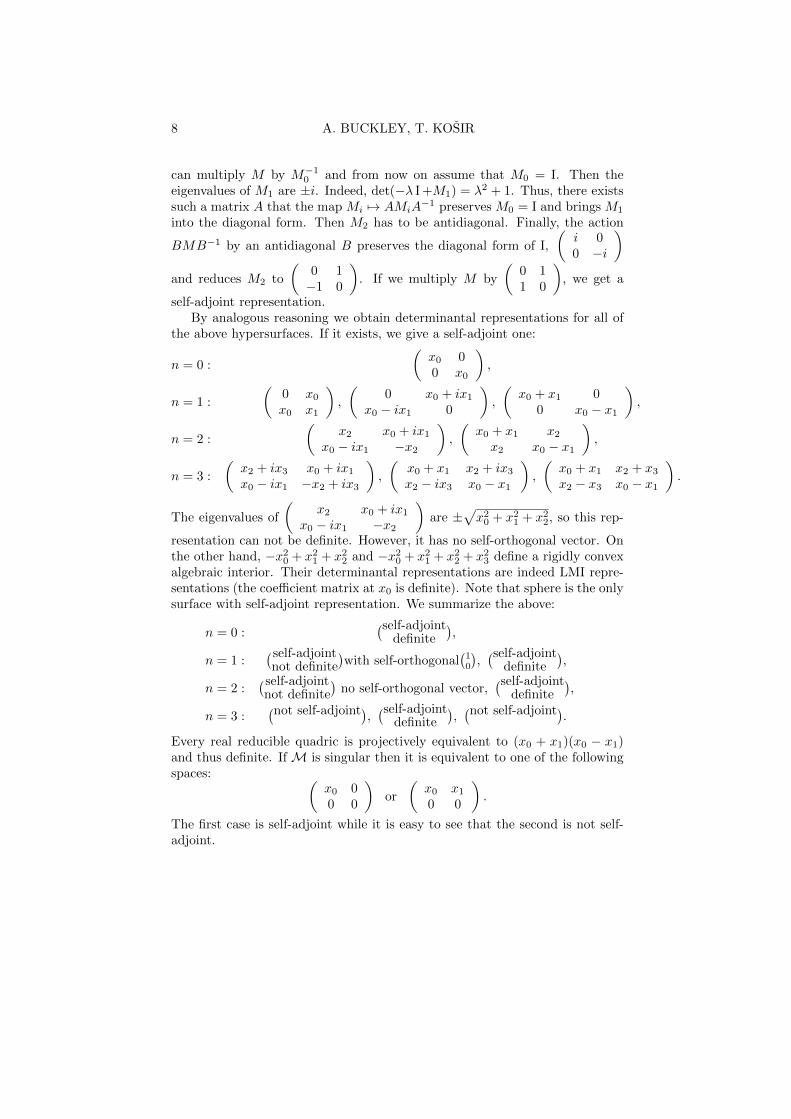
self-adjoint representation.By analogous reasoning we obtain determinantal representations for all of
the above hypersurfaces. If it exists, we give a self-adjoint one:
n = 0 :
(x0 00 x0
),
n = 1 :
(0 x0x0 x1
),
(0 x0 + ix1
x0 − ix1 0
),
(x0 + x1 0
0 x0 − x1
),
n = 2 :
(x2 x0 + ix1
x0 − ix1 −x2
),
(x0 + x1 x2x2 x0 − x1
),
n = 3 :
(x2 + ix3 x0 + ix1x0 − ix1 −x2 + ix3
),
(x0 + x1 x2 + ix3x2 − ix3 x0 − x1
),
(x0 + x1 x2 + x3x2 − x3 x0 − x1
).
The eigenvalues of
(x2 x0 + ix1
x0 − ix1 −x2
)are ±
√x20 + x21 + x22, so this rep-
resentation can not be definite. However, it has no self-orthogonal vector. Onthe other hand, −x20 + x21 + x22 and −x20 + x21 + x22 + x23 define a rigidly convexalgebraic interior. Their determinantal representations are indeed LMI repre-sentations (the coefficient matrix at x0 is definite). Note that sphere is the onlysurface with self-adjoint representation. We summarize the above:
n = 0 :(self-adjoint
definite
),
n = 1 :(self-adjointnot definite
)with self-orthogonal
(10
),(self-adjoint
definite
),
n = 2 :(self-adjointnot definite
)no self-orthogonal vector,
(self-adjointdefinite
),
n = 3 :(not self-adjoint), (self-adjoint
definite
),(not self-adjoint).
Every real reducible quadric is projectively equivalent to (x0 + x1)(x0 − x1)and thus definite. If M is singular then it is equivalent to one of the followingspaces: (
x0 00 0
)or
(x0 x10 0
).
The first case is self-adjoint while it is easy to see that the second is not self-adjoint.

SELF-ADJOINT SETS OF MATRICES 9
4. Regular sets of 3× 3 matrices
In this section we address/answer Question 1, when a regular setM is a simul-taneously self-adjoint. For n ≥ 2 we also assume that M is irreducible. Thereducible case is studied in section 5.
We equate M with M = x0M0 + . . .+ xnMn, where n+ 1 = dimLinRM.Then detM = c F (x0, . . . , xn), 0 6= c ∈ C is a nonzero polynomial in Pn. IfM is equivalent to a self-adjoint representation, the corresponding F has realcoefficients (after factoring out c) and n < 9.
n=0
Since F is nonzero, M0 ∈ GL3(C). Therefore we can always multiply M0 byits inverse to get
1 0 00 1 00 0 1
, which is self-adjoint and definite.
n=1
First check whether det(x0M0 + x1M1) = c F is nonzero and F has real co-efficients. If this holds, a real projective change of coordinates transforms Fto
F = x30 + x1 f(x0, x1)
for some real quadric f . This implies that detM0 6= 0. The group action
x0M0 + x1M1 −→ AM−10 (x0M0 + x1M1)A−1, A ∈ GL3(C)
is the same as the group acting on the pair
(M0,M1) −→ (I, AM−10 M1A−1), A ∈ GL3(C),
which reduces M0 to the identity I and M1 to one of the canonical forms
a 1 00 a 10 0 a
,
a 1 00 a 00 0 b
, or
a 0 00 b 00 0 d
.
Since F is real, either a, b, d ∈ R or a ∈ R, d = b ∈ C. These canonical forms
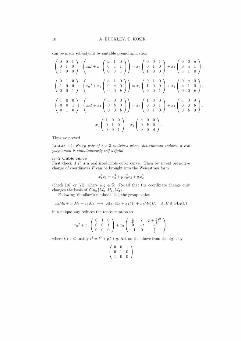
10 A. BUCKLEY, T. KOSIR
can be made self-adjoint by suitable premultiplication: 0 0 10 1 01 0 0
·x0I + x1
a 1 00 a 10 0 a
= x0
0 0 10 1 01 0 0
+ x1
0 0 a0 a 1a 1 0
,
0 1 01 0 00 0 1
·x0I + x1
a 1 00 a 00 0 b
= x0
0 1 01 0 00 0 1
+ x1
0 a 0a 1 00 0 b
,
1 0 00 0 10 1 0
·x0I + x1
a 0 00 b 0
0 0 b
= x0
1 0 00 0 10 1 0
+ x1
a 0 0
0 0 b0 b 0
,
x0
1 0 00 1 00 0 1
+ x1
a 0 00 b 00 0 d
.
Thus we proved
Lemma 4.1. Every pair of 3 × 3 matrices whose determinant induces a realpolynomial is simultaneously self-adjoint.
n=2 Cubic curveFirst check if F is a real irreducible cubic curve. Then by a real projectivechange of coordinates F can be brought into the Weierstrass form
x21x2 = x30 + p x20x2 + q x32
(check [16] or [7]), where p, q ∈ R. Recall that the coordinate change onlychanges the basis of LinR{M0,M1,M2}.
Following Vinnikov’s methods [24], the group action
x0M0 + x1M1 + x2M2 −→ A(x0M0 + x1M1 + x2M2)B, A,B ∈ GL3(C)
in a unique way reduces the representation to
x0I + x1
0 1 00 0 10 0 0
+ x2
t2 l p+ 3
4 t2
0 −t −l−1 0 t
2
,
where t, l ∈ C satisfy l2 = t3 + p t+ q. Act on the above from the right by 0 0 10 1 01 0 0

SELF-ADJOINT SETS OF MATRICES 11
to get
x0
0 0 10 1 01 0 0
+ x1
0 1 01 0 00 0 0
+ x2
p+ 34 t
2 l t2
−l −t 0t2 0 −1
.
This representation is self-adjoint if and only if t is real and l purely imaginary.Vinnikov [24] also proved that all self-adjoint representations of a given curveare of this form.
Therefore we obtain
Proposition 4.2. Let M = x0M0 +x1M1 +x2M2 define a cubic curve x21x2 =x30 + p x20x2 + q x32 with p, q ∈ R. Then M can be in unique way transformed toan equivalent representation x2(p+ 3
4 t2) x1 + x2l x0 + x2
t2
x1 − x2l x0 − x2t 0x0 + x2
t2 0 −x2
,
where l2 = t3 + p t+ q.The set {M0,M1,M2} is simultaneously self-adjoint if and only if
t ∈ R and l ∈ iR.
We conclude the curve case by another characterization that can be easilyused for verification by a computer:
Let M(x0, x1, x2) be a determinantal representation of a cubic curve F . De-fine the corresponding kernel sheaf (or vector bundle if F smooth) ε(x0, x1, x2)along F by
ε(x0, x1, x2) = kerM(x0, x1, x2).
Equivalent determinantal representations clearly induce equivalent vector bun-dles.
The best way to compute a section of ε is as a column of the adjoint matrix
adjM(x0, x1, x2),
whose entries are the signed (n − 1) × (n − 1) minors of M . Since the ad-joint matrix adjM has rank 1, all its columns are proportional along F [24,Proposition 2]. Then
Corollary 4.3. Determinantal representation M(x0, x1, x2) is equivalent toa self-adjoint determinantal representation if and only if
kerM(x0, x1, x2) ≡ kerM∗(x0, x1, x2)
as sheaves (or vector bundles if F is smooth).

12 A. BUCKLEY, T. KOSIR
n=3 Cubic surfaceA generic fourtuple of matrices M induces a determinantal representationM(x0, x1, x2, x3) and a smooth irreducible cubic surface with the equation
F (x0, x1, x2, x3) =1
cdetM = 0, 0 6= c ∈ C.
Singular and reducible sets are considered in Sections 6 and 5, respectively.Every smooth cubic surface can be obtained as a blow-up of P2 in 6 generic
points. We will use the relation between the determinantal representation Mand the six points of the blow-up, which can be found in [14]:
Define a 3× 4 matrix L of linear forms in z1, z2, z3 by
M ·
z0z1z2
= L ·
x0x1x2x3
. (1)
The minors of L form a basis of the 4-dimensiona linear system of plane cubiccurves, which defines the blow-up. At the base points Pi = (ζi, ηi, ξi) ∈ P2, i =1, . . . , 6 the rank of L equals 2 and equals 3 elsewhere. In other words, the rankof L in P = (ζ, η, ξ) ∈ P2 equals 2 if and only if the three planes in P3 withequations
M ·
ζηξ
=
000
intersect in a line. Note that the lines obtained this way are exactly the excep-tional lines of the blow-up [14]. They are mutually skew and we call them thesix skew lines corresponding to determinantal representation M.
In the same way M t determines another set of six skew lines.A configuration of 12 lines with the property that a1, . . . , a6 are mutually
skew, b1, . . . , b6, are mutually skew and ai intersects bj if and only if i 6= j, iscalled a Schlafli double-six and is denoted by(
a1 . . . a6b1 . . . b6
).
In [9, Corollary 3.5] we proved that the lines corresponding to M and M t
form a double-six. More precisely, for a given surface F there is a 1-1 corre-spondence between pairs M, M t and double-sixes on F . From [9, Proposition5.1, Theorem 5.3] it follows
Proposition 4.4. Let M(x0, x1, x2, x3) be a determinantal representation ofa real smooth cubic surface F . Then M is equivalent to a self-adjoint rep-resentation if and only if the double-six corresponding to M,M t is mutually

SELF-ADJOINT SETS OF MATRICES 13
self-conjugate, i.e. (a1 . . . a6b1 . . . b6
)equals to one of the following:
I − st kind:
(a1 a2 a3 a4 a5 a6a1 a2 a3 a4 a5 a6
),
II − nd kind:
(a1 a2 a3 a4 a5 a6a2 a1 a3 a4 a5 a6
),
III − rd kind:
(a1 a2 a3 a4 a5 a6a2 a1 a4 a3 a5 a6
),
IV − th kind:
(a1 a2 a3 a4 a5 a6a2 a1 a4 a3 a6 a5
).
It is easy to collect the above considerations in an answer to our Question 1:
input M;
check cF = detM smooth, F real;
find the corresponding double-six and check its type;
result M is simultaneously self-adjoint if and only if the corresponding double-six is mutually self-conjugate.
It is well known that every smooth surface has exactly 72 nonequivalentdeterminantal representations. The number of self-adjoint representations de-pends on the geometric type of the surface (see [9] and [22]).
The geometry of singular cubic surfaces is also regulated by their configura-tions of lines. Every singular surface is a limit of nonsingular ones [22, page 40].More on these and their determinantal representations can be found in [5, 4].n ≥ 4For a setM with 5 ≤ m ≤ 9 independent matrices it is enough to check if m−3of its 4 dimensional subsets are simultaneously self-adjoint. We will prove thisclaim only for 5-dimensionalM. The generalization to sets of higher dimensionis straightforward.
Theorem 4.5. To a 5-dimensional M we assign a determinantal representa-tion M = x0M0 + · · ·+ x4M4 which defines a cubic threefold F (x0, . . . , x4) inP4.
Let π1 and π2 be hyperplanes in P4 such that F ∩π2 and F ∩π2 are smoothcubic surfaces. Then M is simultaneously self-adjoint if and only if M |π1 andM |π2 are equivalent to some self-adjoint representations.

14 A. BUCKLEY, T. KOSIR
Thus our answer to Question 1 can be extended to n = 4:
input M;
check F real for some 0 6= c ∈ C such that cF = detM ;
find two hyperplanes π1, π2 such that M |π1and M |π2
are determinantal rep-resentations of smooth cubic surfaces;
find the double-sixes corresponding to M |π1 , M |π2 and check their type;
result M is simultaneously self-adjoint if and only if both double-sixes aremutually self-conjugate.
Proof. Both equations πi = 0 can be seen as linear combinations of matricesin M. Then M|πi=0 is a 4 dimensional set. It is obvious that M beingsimultaneously self-adjoint implies thatM|π1=0 andM|π2=0 are simultaneouslyself-adjoint.
Conversely, assume that M |π1=0 and M |π2=0 are equivalent to some self-adjoint representations. We can change the coordinates so that
π1 = {x3 = 0}, π2 = {x4 = 0}
and so that the representation M |{x3=x4=0} defines a Weierstrass cubic curve
x21x2 = x30 + p x0x22 + q x32.
Moreover, as in the case of n = 2, the GL3(C) action from left and right reducesM to the form
x0
0 0 10 1 01 0 0
+x1
0 1 01 0 00 0 0
+x2
p+ 34 t
2 l t2
−l −t 0t2 0 −1
+x3M3+x4M4
for a pair t, l ∈ C satisfying l2 = t3 + p t+ q.By our assumption {M0,M1,M2,M3} are simultaneously self-adjoint. Ob-
serve thatA(M0, M1, M2, M3)B, A,B ∈ GL3(C)
are self-adjoint if and only if
A−1A(M0, M1, M2, M3)BA∗−1
are self-adjoint. Therefore it is enough to check for which
C =
c11 c12 c13c21 c22 c23c31 c32 c33

SELF-ADJOINT SETS OF MATRICES 15
the matrices
M0C =
0 0 10 1 01 0 0
C =
c31 c32 c33c21 c22 c23c11 c12 c13
,
M1C =
0 1 01 0 00 0 0
C =
c21 c22 c23c11 c12 c130 0 0
,
M2C =
? ? (p+ 34 t
2)c13 + lc23 + t2c33
? ? −lc13 − tc23t2c11 − c31
t2c12 − c32 ?
,
M3C
are complex hermitean. From the first two equalities it follows that
c13 = c23 = c12 = 0, c21 = c32 ∈ R, c22 = c11 = c33 ∈ R, c31 ∈ R
and the third equality implies c32 = c31 = 0. Thus C is a multiple of theidentity. This proves that if {M0,M1,M2,M3} are simultaneously self-adjoint,then M3 is complex hermitean.
The same way we prove that if {M0,M1,M2,M4} are simultaneously self-adjoint, then M4 is complex hermitean.
This concludes the proof since the reduced x0M0 +x1M1 +x2M2 +x3M3 +x4M4 is already a self-adjoint representation.
Remark 4.6. Recall that not every cubic threefold has a determinantal rep-resentation with 3 × 3 matrices. Determinantal cubic threefolds are a closed(5 − 2)32 + 2 dimensional subvariety in the
(3+5−1
3
)dimensional variety of all
cubic threefolds.
For n > 4 the same argument works. Without loss of generality we onlyneed to test the sets
{M0,M1,M2,Mk}, k = 3, . . . , n.
5. Reducible sets
Now, we assume that a subset M is regular and reducible. The correspondingpolynomial F = detM is a reducible polynomial. It can be a product ofan irreducible quadratic and a linear polynomial or a product of three linearfactors (counting multiplicities). We apply a result of Kerner and Vinnikov [19,

16 A. BUCKLEY, T. KOSIR
Thm. 3.1], which tells us that the corresponding kernel sheaf kerM(x1, . . . , xn)is globally a direct sum of kernel sheaves over distinct irreducible componentsof F . This can be viewed as a matrix version of a generalized M. Noether’sAF +BG Theorem [1, p. 139].
Lemma 5.1. If M is a regular and reducible subspace of 3× 3 matrices that isself-adjoint then dimRM≤ 5.
Proof. First suppose that F = detM has two distinct irreducible factors. Onehas to be linear of multiplicity 1. So F = lq, where l is linear, q quadratic andl does not divide q. Then the kernel sheaf of M is globally decomposable by[19, Thm. 3.1], i. e.,
M =
(M(1) 0
0 M(2)
),
where detM(1) = cl and detM(2) = c−1q for a nonzero scalar c. We saw inSection 3 that the dimension over R of a selfadjoint M ⊂ C2×2 is at most 4.Hence dimM≤ 5.
Assume next that F is of the form l3 for some linear form l. Without losswe can take F = x30. Further we can assume that M0 = I. Then any othermatrix Mi in the basis of M is nilpotent. The maximal possible dimensionover C of a subspace of 3 × 3 nilpotent matrices is 3 (see [15]). Thus it is atmost 6 over R. A straightforward analysis then shows that the selfadjointnesscondition implies that also dimRM = 3. If the dimension over C is at most 2then over R it is at most 4. Thus it follows that dimM≤ 5.
The case n = 0 and n = 1 were studied in Section 4.
Then an elementary analysis of all possible cases using the results of Sec-tion 3 yields a complete list of all possible cases. It is straightforward butcumbersome to write down, so we omit it.
6. Singular Sets of 3× 3 matrices
It remains to consider sets M with determinant constantly 0. In other words,rankM = x1M1 + · · · + xnMn ≤ 2 for all x1, . . . , xn ∈ R. In this case theGL3(C) action transforms each Mi separately into either 1 0 0
0 0 00 0 0
or
0 1 01 0 00 0 0
.
We say that M is of rank i, i = 1, 2, if M is singular, rankN ≤ i for allN ∈M and rankN = i for at least one N ∈M.

SELF-ADJOINT SETS OF MATRICES 17
Proposition 6.1. Suppose that M1,M2, . . . ,Mn is a basis of a subspace Mwhich is of rank 1. ThenM is simultaneously self-adjoint if and only if x1M1+· · ·+ xnMn is equivalent to m11 0 0
0 0 00 0 0
,
where m11 is a real linear form in x1, . . . , xn.
Proposition 6.2. Suppose that M1,M2, . . . ,Mn is a basis of a subspace Mwhich is of rank 2 and that rankM1 = 2. Then M is simultaneously self-adjoint iff x1M1 + · · ·+ xnMn is equivalent to one of the following: x1 +m11 m12 0
m12 x1 +m22 00 0 0
,
m11 x1 +m12 0x1 +m12 m22 0
0 0 0
,
m11 x1 +m12 m13
x1 +m12 0 0m13 0 0
or −γm11 x1 + iδm11 −m12 im11
x1 + iγm22 −m12 δm22 m22
−im11 m22 0
.
Here mij are linear forms in x2, . . . , xn, m11 and m22 are real. Moreover, inthe last matrix above we have γ, δ ∈ R and m12 −m12 = i(γm22 + δm11).
7. Definite linear combinations of matrices
In this section we examine Question 2, when a set of 3× 3 matrices is definite.We only need to consider the case of M regular. In order to stress that theelements of M are complex hermitean, we denote them by Ui. As before,equate M with U = x0U0 + . . .+ xnUn, where n+ 1 = dimLinRM.
Our question is whether U is a LMI representation. In other words, dothere exist k0, . . . , kn ∈ R such that
k0U0 + k1U1 + · · ·+ knUn > 0.
The property of being definite is an open condition. More precisely, all n+ 1–tuples (k0, . . . , kn) inside the spectrahedron (hyperbolicity set) satisfy U(k0, · · · , kn) >0. Small perturbations of ki or of the entries in Ui preserve definiteness, there-fore we can afford small errors occuring by numeric computations.
Throughout this section we will need the following elementary result.

18 A. BUCKLEY, T. KOSIR
Lemma 7.1. Let λ1, λ2, λ3 ∈ R.Then λ1 > 0, λ2 > 0, λ3 > 0 if and only if
λ1 + λ2 + λ3 > 0, λ1λ2 + λ1λ3 + λ2λ3 > 0, λ1λ2λ3 > 0.
The same way λ1 < 0, λ2 < 0, λ3 < 0 if and only if
λ1 + λ2 + λ3 < 0, λ1λ2 + λ1λ3 + λ2λ3 > 0, λ1λ2λ3 < 0.
Proof. We will prove the first statement (the second proof is the same). Im-plication ⇒ is obvious. Conversely, assume that λ1 > 0, λ2 < 0, λ3 < 0. Wewill prove that this implies either λ1 + λ2 + λ3 < 0 or λ1λ2 + λ1λ3 + λ2λ3 < 0,which finishes the proof.
Indeed, if λ1 + λ2 + λ3 ≥ 0, then
λ1λ2 + λ1λ3 + λ2λ3 =λ1(λ2 + λ3) + λ2λ3 ≤−(λ2 + λ3)2 + λ2λ3 =−λ22 − λ23 − λ2λ3 < 0,
since λ1 ≥ −(λ2 + λ3) > 0.
Consider now U = (uij)1≤i,j≤3, a complex hermitean matrix with eigenval-ues
λ1, λ2, λ3 ∈ R.
By Lemma 7.1 the signs of λi can be read from the characteristic polynomial
det(ΛI − U) = (Λ− λ1)(Λ− λ2)(Λ− λ3)= Λ3 − Λ2(λ1 + λ2 + λ3) + Λ(λ1λ2 + λ1λ3 + λ2λ3)− λ1λ2λ3.
On the other hand
det(ΛI − U) =
Λ3 − Λ2(u11 + u22 + u33) + (2)
Λ(u11u22 − u12u12 + u11u33 − u13u13 + u22u33 − u23u23)− detU.
Like in Section 4 we consider different n separately.n = 0Calculate the eigenvalues of U0. If they are all of the same sign, then U0 isdefinite.n = 1Recall that the coordinates in x0U0 + x1U1 can be chosen so that
det(x0U0 + x1U1) = x30 + x0x1(· · · ).

SELF-ADJOINT SETS OF MATRICES 19
In particular detU0 6= 0 and detU1 = 0.First check if U0 is already definite. If not, we need to check whether
U0 + tU1
is definite for some t ∈ R. The characteristic polynomial of U0 + tU1 by (2)equals
Λ3 − Λ2 trace(U0 + tU1) + Λ q(t)− det(U0 + tU1),
where trace(U0 + tU1) is a linear, q(t) is a quadratic and det(U0 + tU1) is acubic polynomial in t. It is easy to check from their graphs if there exists t ∈ Rfor which either
trace(U0 + tU1) > 0, q(t) > 0, det(U0 + tU1) > 0
ortrace(U0 + tU1) < 0, q(t) > 0, det(U0 + tU1) < 0.
If such t exists, then U0+tU1 is definite by Lemma 7.1. Otherwise it is indefinite.n = 2For cubic curves we use the following beautiful result
Theorem 7.2. [24, Theorems 8 & 9] Let
U = x0U0 + x1U1 + x2U2
be a self-adjoint determinantal representation of a smooth cubic curve withequation x21x2 = x30 + px20x2 + qx32. There exists a unique P ∈ GL3(C) forwhich either PUP ∗ or −PUP ∗ equals
x0
0 0 10 1 01 0 0
+ x1
0 1 01 0 00 0 0
+ x2
p+ 34 t
2 l t2
−l −t 0t2 0 −1
.
Here t ∈ R, l ∈ iR and l2 = t3 + pt+ q.Observe that
l2 = t3 + pt+ q
defines an affine curve C in R2 ≡ C. When equation E : t3 + pt + q = 0has 3 real solutions, C consists of two components, one compact and the othernon-compact. When E has a pair of complex conjugate solutions, C consistsof a single non-compact component.
The representation U is definite if and only if the corresponding point (t, l)lies on the compact component of C. Moreover, U is either definite or thecoefficient matrices U0, U1, U2 have a common self-orthogonal vector.
The same result holds for representations of singular irreducible curves [7].
20 A. BUCKLEY, T. KOSIR
Corollary 7.3. A pair of complex hermitean matrices U0, U1 is either definiteor U0, U1 have a common self-orthogonal vector.
Proof. Let U0, U1 have a common self-orthogonal vector v ∈ C3. Then x0U0 +x1U1 is indefinite, because by definition vU0v
∗ = vU1v∗ = 0.
Next assume that x0U0 + x1U1 is indefinite. Find a matrix U2 such that(after a real projective change of coordinates)
det(x0U0 + x1U1 + x2U2)
is a Weierstrass curve and the graph in R2 only has one non-compact compo-nent. Then U0, U1, U2 have a common self-orthogonal vector by Theorem 7.2.
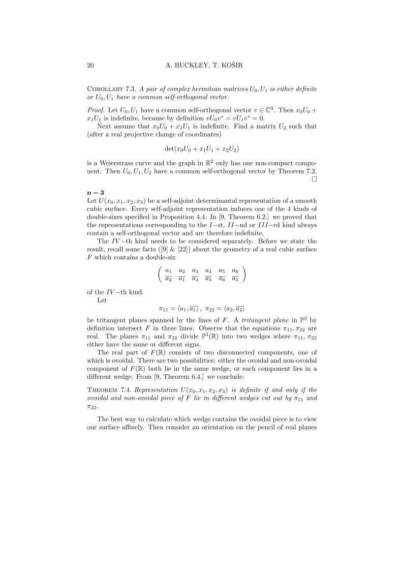
n = 3Let U(x0, x1, x2, x3) be a self-adjoint determinantal representation of a smoothcubic surface. Every self-adjoint representation induces one of the 4 kinds ofdouble-sixes specified in Proposition 4.4. In [9, Theorem 6.2.] we proved thatthe representations corresponding to the I−st, II−nd or III−rd kind alwayscontain a self-orthogonal vector and are therefore indefinite.
The IV−th kind needs to be considered separately. Before we state theresult, recall some facts ([9] & [22]) about the geometry of a real cubic surfaceF which contains a double-six(
a1 a2 a3 a4 a5 a6a2 a1 a4 a3 a6 a5
)of the IV−th kind.
Letπ11 = 〈a1, a1〉 , π22 = 〈a2, a2〉
be tritangent planes spanned by the lines of F . A tritangent plane in P3 bydefinition intersect F in three lines. Observe that the equations π11, π22 arereal. The planes π11 and π22 divide P3(R) into two wedges where π11, π22either have the same or different signs.
The real part of F (R) consists of two disconnected components, one ofwhich is ovoidal. There are two possibilities: either the ovoidal and non-ovoidalcomponent of F (R) both lie in the same wedge, or each component lies in adifferent wedge. From [9, Theorem 6.4.] we conclude:
Theorem 7.4. Representation U(x0, x1, x2, x3) is definite if and only if theovoidal and non-ovoidal piece of F lie in different wedges cut out by π11 andπ22.
The best way to calculate which wedge contains the ovoidal piece is to viewour surface affinely. Then consider an orientation on the pencil of real planes

SELF-ADJOINT SETS OF MATRICES 21
with the axis π11 ∩ π22. The axis is a real line, since π11 and π22 intersect in areal line on F .
It follows from the above, that we can answer Question 2 using the followingalgorithm:
input {U0, . . . , U3};
check all Ui complex hermitean, detU smooth;
find the corresponding double-six and check its type;
if of kind I, II or III then {Ui}i=0,...,3 is indefinite;
else construct the corresponding tritangent planes π11, π22;
check which wedge contains the ovoidal and nonovoidal parts of the surfaceby rotating real planes around the axis π11 ∩ π22.
In the case of surfaces of the IV –th kind indefiniteness does not imply theexistence of a self-orthogonal vector. It is easy to construct a self-adjoint rep-resentation which is not definite and has no self-orthogonal vector [9, Example6.5].n ≥ 4To a n+1 dimensionalM we assign a self-adjoint determinantal representation
U = x0U0 + · · ·+ xnUn
which defines a real cubic hypersurface F (x0, . . . , xn) in Pn. With growingn it is more likely that the representation becomes definite. On the otherhand, the geometry of higher dimensional cubic hypersurfaces gets much morecomplicated. Note that for U to be a LMI representation, F = 0 needs to havea compact ”ovoidal” piece. This is exactly the hyperbolicity set (spectrahedronor rigidly convex algebraic interior in the affine setting).
Consider the eigenvalues λi(x0, . . . , xn) of U . They are the solutions ofthe characteristic polynomial det(ΛI − U) which we computed in (2). ByLemma 7.1, U is definite if and only if there exist k0, . . . , kn ∈ R such that
L : u11 + u22 + u33,
Q : u11u22 − u12u12 + u11u33 − u13u13 + u22u33 − u23u23,F : detU
evaluated in (k0, . . . , kn) are all strictly positive.Note that uij are linear functions of x0, . . . , xn. Then L = 0 defines a real
hyperplane, Q = 0 a quadratic form and F = 0 our cubic in Pn. Write
Q = (x0, . . . , xn)S (x0, . . . , xn)t,

22 A. BUCKLEY, T. KOSIR
where S is a real symmetric n + 1 × n + 1 matrix. Observe that S negativedefinite implies Q ≤ 0 for all values of x0, . . . , xn. In this case U can not bedefinite.
On the other hand, S positive definite implies Q > 0 for all x0, . . . , xn 6=0n+1. Since L = 0 and F = 0 always intersect in Rn+1 (a real cubic equationhas a real solution), there exist k0, . . . , kn ∈ R in which L > 0, F > 0. In thiscase U is definite.
The last option we need to consider is the case when S is indefinite. ThenQ = 0 is a nonempty conic in P(Rn+1). Recall that P(Rn+1) can be dividedinto two parts by the equations of L and F : points in which L,F are both ofthe same sign and points in which L,F have different sign. Denote the firstpart L · F > 0 and the second part L · F < 0. Under these assumptions we get
Proposition 7.5. The representation U is indefinite if and only if the conicQ = 0 and its interior Q > 0 are entirely included in the L · F < 0 part.
In particular, Q ∩ L must be empty, which implies that Q|L=0 is a definitequadratic form.
Proof. The statement follows easily from Figure 1.
The interior of the sphere represents Q > 0. Then U is indefinite if andonly if L and F have different signs along the whole area defined by Q > 0. Inother words, U is definite if either
• Q = 0 intersects L = 0,
• Q = 0 intersects F = 0,
• Q > 0 intersects the part L · F > 0.
We finish the section by summarizing the above observations:
input {Ui}i=0,...,n complex hermitean;
find L = traceU, Q = (x0, . . . , xn)S(x0, . . . , xn)t, F = detU ;
if S negative definite, then U indefinite;
if S positive definite, then U definite;
else check the position and sign of Q with respect to the parts L · F > 0 andL · F < 0. Then use Proposition 7.5.

SELF-ADJOINT SETS OF MATRICES 23
Q<0L·F <0
Q<0L·F >0
Figure 1: L and F always intersect.
References
[1] E. Arbarello, M. Cornalba, P.A. Griffiths, and J. Harris, Geometry of

24 A. BUCKLEY, T. KOSIR
Algebraic Curves. Vol. I, Springer-Verlag, 1985.[2] A. Beauville, Determinantal hypersurfaces, Michigan Math. J. 48 (2000), 39–
63.[3] P. Branden, Obstructions to determinantal representability, Adv. Math. 226
(2011), 1202–1212.[4] M. Brundu and A. Logar, Classification of cubic surfaces with computational
methods, Quaderni Matematici, Serie II, No. 375 (1996), Univ. of Trieste.[5] M. Brundu and A. Logar, Parametrization of the orbits of cubic surfaces,
Transformation Groups. 3, No. 3 (1998), 209–239.[6] A. Buckley and T. Kosir, Construction of self-adjoint determinantal repre-
sentations of smooth cubic surfaces, Proceedings of the 6th EUROSIM Congresson Modelling and Simulation. (Ljubljana, Slovenia.), 2007.
[7] A. Buckley and T. Kosir, Determinantal representations of smooth cubicsurfaces, Geometriae Dedicata 125 (2007), 115–140.
[8] A. Buckley and T. Kosir, Plane curves as pfaffians, Annali della Scuolanormale superiore di Pisa, Classe di scienze. 10, iss. 2 (2011), 363–388.
[9] A. Buckley and T. Kosir, Determinantal representations of cubic curves,Conference on Geometry: Theory and Applications. (University of Ljubljana.),2013.
[10] F. Catanese, Babbage’s conjecture, contact of surfaces, symmetric determinan-tal varieties and applications, Inventiones Mathematicae. 63, Nu. 3 (1981),433–465.
[11] R. J. Cook and A. D. Thomas, Line bundles and homogeneous matrices,Quart. J. Math. Oxford Ser. (2) 30 (1979), 423–429.
[12] L. E. Dickson, Determination of all general homogeneous polynomials express-ible as determinants with linear elements, Trans. Amer. Math. Soc. 22 (1921),167–179.
[13] I. V. Dolgachev, Classical algebraic geometry: A modern view, CambridgeUniversity Press., 2012.
[14] A. Geramita, Lectures on the non-singular cubic surfaces in P3, Queen’s Papersin Pure and Applied Math. Queen’s University, Kingston, Canada, A1–A99,1989.
[15] M. Gerstenhaber, On nilalgebras and varieties of nilpotent matrices III, Ann.of Math. 70 (2) (1959), 167–205.
[16] J. Harris, Galois groups of enumerative problems, Duke Math. J. 46 (4) (1979),685–724.
[17] J.W. Helton, S.A. McCullough, and V. Vinnikov, Noncommutative con-vexity arises from linear matrix inequalities, Journal of Functional Analysis240 (1) (2006), 105–191.
[18] J.W. Helton and V. Vinnikov, Linear matrix inequality representation ofsets, Comm. Pure Appl. Math. 60 (5) (2007), 654–674.
[19] D. Kerner and V. Vinnikov, Determinantal representations of singular hy-persurfaces in Pn, Adv. Math. 231 (2012), 1619–1654.
[20] J. Piontkowski, Linear symmetric determinantal hypersurfaces, MichiganMath. J. 54 (1) (2006), 117155.
[21] D. Plaumann, B. Sturmfels, and C. Vinzant, Quartic curves and their

SELF-ADJOINT SETS OF MATRICES 25
bitangents, J. Symb. Comput. 46 (6) (2011), 712–733.[22] B. Segre, The non-singular cubic surfaces, Oxford University Press., 1942.[23] F. Tanturri, Pfaffian representations of cubic surfaces, Geom. Dedicata 168
(2014), 69–86.[24] V. Vinnikov, Self-adjoint determinantal representations of real irreducible cu-
bics, Operator Theory: Advances and Applications. 19 (1986), 415–442.[25] V. Vinnikov, Complete description of determinantal representations of smooth
irreducible curves, Lin. Alg. Appl. 125 (1989), 103–140.[26] V. Vinnikov, Self-adjoint determinantal representations of real plane curves,
Math. Anal. 296 (1993), 453–479.[27] V. Vinnikov, LMI representations of convex semialgebraic sets and determi-
nantal representations of algebraic hypersurfaces: Past, present, and future, Op-erator Theory: Advances and Applications. 222 (2012), 325–349.
Authors’ addresses:
Anita BuckleyFaculty of Mathematics and Physics, University of Ljubljana, Jadranska 19, 1000 Ljubljana,Slovenia.E-mail: [email protected]
Tomaz KosirFaculty of Mathematics and Physics, University of Ljubljana, Jadranska 19, 1000 Ljubljana,Slovenia.E-mail: [email protected]
Received December 12, 2014Revised March 5, 2015