Simultaneously Fitting and Segmenting Multiple- Structure ...
14
Simultaneously Fitting and Segmenting Multiple- Structure Data with Outliers Hanzi Wang a, b, c , Senior Member, IEEE, Tat-Jun Chin b , Member, IEEE and David Suter b , Senior Member, IEEE Abstract—We propose a robust fitting framework, called Adaptive Kernel-Scale Weighted Hypotheses (AKSWH), to segment multiple- structure data even in the presence of a large number of outliers. Our framework contains a novel scale estimator called Iterative Kth Ordered Scale Estimator (IKOSE). IKOSE can accurately estimate the scale of inliers for heavily corrupted multiple-structure data and is of interest by itself since it can be used in other robust estimators. In addition to IKOSE, our framework includes several original elements based on the weighting, clustering, and fusing of hypotheses. AKSWH can provide accurate estimates of the number of model instances, and the parameters and the scale of each model instance simultaneously. We demonstrate good performance in practical applications such as line fitting, circle fitting, range image segmentation, homography estimation and two-view based motion segmentation, using both synthetic data and real images. Index Terms—Robust Statistics, Model Fitting, Scale Estimation, Kernel Density Estimation, Multiple Structure Segmentation. —————————— ————————— 1 INTRODUCTION e consider the setting where one is given some data and within that data there are several structures of interest: where one knows the general form of a pa- rametric model that these structures “fit”. We are motivated by applications in computer vision: such as line and circle finding in images, homography/fundamental matrix estima- tion, optical flow calculation, range image segmentation, mo- tion estimation and segmentation. We adopt the paradigm that these models (line, circle, homography, fundamental matrix, etc.) can be found by robust fitting. “Robust” because the data contains outliers or pseudo-outliers (the latter refers to the fact that data belonging to one structure is usually an outlier to any other structure) [2, 3]. Traditional robust approaches such as M-estimators [4], LMedS [5] and LTS [6], cannot tolerate more than 50% of out- liers. This is a severe limitation when these approaches are ap- plied to multiple-structure data, where outliers (and pseudo- outliers to any structure) are a large fraction of the data. A number of robust approaches claim to tolerate more than 50% of outliers: HT [7], RHT [8], RANSAC [9], MSAC [10], MUSE [11], MINPRAN [12], ALKS [13], RESC [14], pbM [15], HBM [16], ASSC [2], ASKC [17], etc. These cannot be considered as complete solutions to the above problem be- cause they either require a sequential “fitting-and-removing” procedure (i.e., sequentially estimate the parameters of one model instance, dichotomize the inliers belonging to that model instance from outliers, and remove the inliers from data) or some form of further analysis, in the case of HT/RHT, to segment multiple-modes in “Hough space” (i.e., model parameter space). Moreover, the methods (typified by RANSAC and related estimators) generally require one or more parameters related to the scale of inliers (or equivalent, the error tolerance) to be either specified by the user or esti- mated by a separate procedure. Further, we note that the sequential “fitting-and-removing” procedure has limitations: (1) if the parameters or the scale of a model instance is incorrect, the inliers of the remaining model instances may be wrongly removed, and the inliers to the current model instance may be incorrectly left in. This will lead to inaccurate estimation of the remaining model instances in the following steps; (2) Also, the sequential “fit- ting-and-removing” procedure is not computationally efficient because it requires generating a large number of hypotheses in each step. Alternatives have been proposed but these too have limi- tations. MultiRANSAC [18] requires the user to specify both the number of model instances and the inlier scales. GPCA [19] is restricted to fitting linear subspaces, and requires that the user specifies the number of populations. Moreover, GPCA becomes problematic for data involving outliers and a large number of structures. MS (Mean Shift) [20, 21] and its variants [22, 23], at- tempt to detect/estimate model instances by finding peaks in parameter space; however, this becomes very difficult when the inlier noise is high and/or the percentage of outliers is high. Moreover, it is not trivial to find a global optimal bin size for HT/RHT or an optimal bandwidth for the MS-based approaches to both achieve accurate results and correctly localize multiple significant peaks in parameter space. RHA [24] is predicated on an interesting property of resi- duals (to hypothesized fits) when the model instances are parallel to each other, however any guarantee of performance when models are not parallel relies on (limited) empirical sup- port. Also, RHA requires the user to specify both the histogram bin size (limitation shared by HT/RHT and others) and a thre- shold for selecting the significant local peaks corresponding to the model instance number. A Jaccard-distance linkage (J-linkage) based agglomera- tive clustering technique [25] is more effective than RHA when model instances are not parallel. However, they dicho- tomize inliers/outliers by a user-specified inlier scale, which is not known in practice. Like RANSAC, the performance of J- linkage greatly depends on the input inlier scale. In the kernel fitting (KF) approach [26]: gross outliers are identified first and removed, and then the multiple structures are estimated in parallel. Unlike J-linkage and RANSAC, KF does not require a user to specify the inlier scale. However, KF uses a step size h in computing the ordered residual kernel. KF also requires a user to specify the relative weighting ratio be- tween fitting error and model complexity in implementing the model selection procedure. We note that although the MS-based approaches [20, 22, 23], RHA [24], J-linkage [25] and KF [26] claim to be able to detect the number of model instances, they all require some user-specified thresholds whose values are crucial in deter- mining the number of model instances (e.g.,[23] suggests for the MS-based approaches that the significant peaks are ———————————————— • a School of Information Science and Technology, Xiamen University, Fujian, 361005, China; E-mail: [email protected]; • b School of Computer Science, The University of Adelaide, North Terrace, South Australia 5005, Australia. E-mail: {tatjun-chin, david.suter}@ ade- laide.edu.au • c Fujian Key Laboratory of the Brain-like Intelligent Systems (Xiamen University), Fujian, China, 361005 W
Transcript of Simultaneously Fitting and Segmenting Multiple- Structure ...

Simultaneously Fitting and Segmenting Multiple-Structure Data with Outliers
Hanzi Wanga, b, c , Senior Member, IEEE, Tat-Jun Chinb, Member, IEEE and David Suterb, Senior Member, IEEE
Abstract—We propose a robust fitting framework, called Adaptive Kernel-Scale Weighted Hypotheses (AKSWH), to segment multiple-structure data even in the presence of a large number of outliers. Our framework contains a novel scale estimator called Iterative Kth Ordered Scale Estimator (IKOSE). IKOSE can accurately estimate the scale of inliers for heavily corrupted multiple-structure data and is of interest by itself since it can be used in other robust estimators. In addition to IKOSE, our framework includes several original elements based on the weighting, clustering, and fusing of hypotheses. AKSWH can provide accurate estimates of the number of model instances, and the parameters and the scale of each model instance simultaneously. We demonstrate good performance in practical applications such as line fitting, circle fitting, range image segmentation, homography estimation and two-view based motion segmentation, using both synthetic data and real images.
Index Terms—Robust Statistics, Model Fitting, Scale Estimation, Kernel Density Estimation, Multiple Structure Segmentation.
———————————————————1 INTRODUCTION
e consider the setting where one is given some data and within that data there are several structures of interest: where one knows the general form of a pa-
rametric model that these structures “fit”. We are motivated by applications in computer vision: such as line and circle finding in images, homography/fundamental matrix estima-tion, optical flow calculation, range image segmentation, mo-tion estimation and segmentation. We adopt the paradigm that these models (line, circle, homography, fundamental matrix, etc.) can be found by robust fitting. “Robust” because the data contains outliers or pseudo-outliers (the latter refers to the fact that data belonging to one structure is usually an outlier to any other structure) [2, 3].
Traditional robust approaches such as M-estimators [4], LMedS [5] and LTS [6], cannot tolerate more than 50% of out-liers. This is a severe limitation when these approaches are ap-plied to multiple-structure data, where outliers (and pseudo-outliers to any structure) are a large fraction of the data.
A number of robust approaches claim to tolerate more than 50% of outliers: HT [7], RHT [8], RANSAC [9], MSAC [10], MUSE [11], MINPRAN [12], ALKS [13], RESC [14], pbM [15], HBM [16], ASSC [2], ASKC [17], etc. These cannot be considered as complete solutions to the above problem be-cause they either require a sequential “fitting-and-removing” procedure (i.e., sequentially estimate the parameters of one model instance, dichotomize the inliers belonging to that model instance from outliers, and remove the inliers from data) or some form of further analysis, in the case of HT/RHT, to segment multiple-modes in “Hough space” (i.e., model parameter space). Moreover, the methods (typified by RANSAC and related estimators) generally require one or more parameters related to the scale of inliers (or equivalent, the error tolerance) to be either specified by the user or esti-mated by a separate procedure.
Further, we note that the sequential “fitting-and-removing” procedure has limitations: (1) if the parameters or the scale of a model instance is incorrect, the inliers of the remaining model instances may be wrongly removed, and the inliers to the current model instance may be incorrectly left in. This will lead to inaccurate estimation of the remaining model
instances in the following steps; (2) Also, the sequential “fit-ting-and-removing” procedure is not computationally efficient because it requires generating a large number of hypotheses in each step.
Alternatives have been proposed but these too have limi-tations. MultiRANSAC [18] requires the user to specify both the number of model instances and the inlier scales. GPCA [19] is restricted to fitting linear subspaces, and requires that the user specifies the number of populations. Moreover, GPCA becomes problematic for data involving outliers and a large number of structures. MS (Mean Shift) [20, 21] and its variants [22, 23], at-tempt to detect/estimate model instances by finding peaks in parameter space; however, this becomes very difficult when the inlier noise is high and/or the percentage of outliers is high. Moreover, it is not trivial to find a global optimal bin size for HT/RHT or an optimal bandwidth for the MS-based approaches to both achieve accurate results and correctly localize multiple significant peaks in parameter space.
RHA [24] is predicated on an interesting property of resi-duals (to hypothesized fits) when the model instances are parallel to each other, however any guarantee of performance when models are not parallel relies on (limited) empirical sup-port. Also, RHA requires the user to specify both the histogram bin size (limitation shared by HT/RHT and others) and a thre-shold for selecting the significant local peaks corresponding to the model instance number.
A Jaccard-distance linkage (J-linkage) based agglomera-tive clustering technique [25] is more effective than RHA when model instances are not parallel. However, they dicho-tomize inliers/outliers by a user-specified inlier scale, which is not known in practice. Like RANSAC, the performance of J-linkage greatly depends on the input inlier scale.
In the kernel fitting (KF) approach [26]: gross outliers are identified first and removed, and then the multiple structures are estimated in parallel. Unlike J-linkage and RANSAC, KF does not require a user to specify the inlier scale. However, KF uses a step size h in computing the ordered residual kernel. KF also requires a user to specify the relative weighting ratio be-tween fitting error and model complexity in implementing the model selection procedure.
We note that although the MS-based approaches [20, 22, 23], RHA [24], J-linkage [25] and KF [26] claim to be able to detect the number of model instances, they all require some user-specified thresholds whose values are crucial in deter-mining the number of model instances (e.g.,[23] suggests for the MS-based approaches that the significant peaks are
———————————————— • aSchool of Information Science and Technology, Xiamen University, Fujian,
361005, China; E-mail: [email protected]; • bSchool of Computer Science, The University of Adelaide, North Terrace,
South Australia 5005, Australia. E-mail: {tatjun-chin, david.suter}@ ade-laide.edu.au
• c Fujian Key Laboratory of the Brain-like Intelligent Systems (Xiamen University), Fujian, China, 361005
W

2 IEEE TRANSACTIONS ON PATTERN ANALYSIS AND MACHINE INTELLIGENCE, MANUSCRIPT ID: TPAMI-2010-07-0509
selected if the first N modes clearly dominate the (N+1)th mode but the authors do not discuss how to judge if the Nth mode dominates the (N+1)th mode, nor specify a threshold value for the judgment. RHA [24] uses a threshold to eliminate spurious peaks in the residual histogram while J-linkage determines the number of model instances by selecting sig-nificant bins of the hypothesis histogram whose value is larger than a user-specified threshold. The value of the step size h and the weighting ratio used in KF has a significant influence on determining the number of model instances [26]). To detect the number of model instances is still one of the most difficult things in model fitting [27, 28].
Our approach is based on sampling parameter space, Sec. 3.1, (since each point in this space is a potential model, we also call this “hypothesis space”) – this starting point is similar to HT/RHT. Fig. 1 illustrates the basic steps – starting from weighting the hypotheses samples in Fig. 1 (c). A key element in efficiency is that we prune this space (Sec. 3.3 ), using a principled information theoretic criteria, after weighting each hypothesis so as to emphasise likely candidates (Sec. 3.2). Since multiple surviving (hence highly likely to be approxi-mations to a true structure) samples in hypothesis space may actually come from the same structure, we cluster the surviving hypotheses (Sec. 3.4) using an approach inspired by J-linkage (but with very important differences – see the discussion therein), that, whilst providing an advance to-wards good clusters, does have a tendency to over-segment the clusters (Fig. 1 (d)). Thus we refine these clusters (Sec. 3.5) using, again, a principled information theoretic criterion (Fig. 1 (e)).
Like most algorithms, our approach is crucially dependent on the quality of the output of the first stage – in our case, the weighting of hypotheses before pruning. Our weighting is based on the notion that a “good hypothesis” is one that “explains well” the data “around it”. In essence, this notion, like in many methods, is based upon an analysis of the smaller residuals (if the model is a true one then the data giving rise to these residuals would likely “belong” to that model) that es-sentially characterises an effective inlier scale. Here we do two things – we improve the scale estimator KOSE [13] (the new scale estimator is called IKOSE – Sec. 2.2) and we also improve on the scoring function (Sec. 3.2) used in [17, 29] (firstly with a better estimate of scale and secondly in how we use that scale). Our main contribution is that we develop a framework (AKSWH) that simultaneously fits all models to multiple-structured data and segments the data. In the framework, the relevant quantities (the parameters, the scales and the number of model instances) are determined automatically. In so doing, we have original contributions in various building blocks: (1) we propose a robust scale estimator called Iterative Kth Ordered Scale Estimator (IKOSE), which can accurately estimate the scale of inliers for heavily corrupted data with multiple structures. IKOSE is of interest by itself since it can be a com-ponent in any robust approach that uses a data driven scale estimate; (2) We propose an effective hypotheses weighting function that contributes to rapid elimination of poor hypo-theses. Our combination of this with a (fully automatic) en-tropy thresholding approach lead to high computational effi-ciency; (3) From that point, our algorithm uses the relatively common “divide into small clusters (i.e., over segmented clusters) and then merge” procedure but with a couple of novel features such as effectively using a Jaccard-distance based clustering algorithm refined by the use of mutual information theory to fuse the over-segmented clusters. (e.g., when the inlier noise of a structure is large, there may be more than one cluster corresponding to the structure). Overall, as a result of these
innovations, AKSWH does not require the user to specify the number of structures nor the inlier scale of each model instance. AKSWH can deal with multiple-structured data heavily corrupted with out-liers. Our experimental results show that the proposed IKOSE and AKSWH outperform competing approaches in both scale estimation and model fitting.
We are not claiming to have solved the impossible – a completely automated system that will determine exactly how many structures there are in a scene, and recover all these structures with high precision and reliability. Such is impossible because it depends upon what is considered as an important structure (a wall is a single plane at one resolution but a collection of closely aligned planes at finer resolution). Rather what we are claiming is that: when one have a num-ber of roughly comparable sized structures in the scene, our approach will (and to an extent better than other competitors) determine not only the number of those structures but reliably fit and segment them.
The remainder of the paper is constructed as follows: in Sec. 2, we review existing scale estimation techniques; and then propose a novel scale estimator and evaluate its perfor-mance. In Sec. 3, we develop the main components of the proposed approach. We put all the developed components together to obtain a complete framework in Sec. 4. In Sec. 5 we provide experimental results (with both synthetic and real data), and we give a concluding discussion in Sec. 6.
2 SCALE ESTIMATION Scale estimation plays an important role in robust model fit-ting and segmentation. The accuracy of the scale estimate (or error tolerance) greatly affects the performance of many ro-bust estimators such as RANSAC, HT, RHT, multiRANSAC, M-estimators, MSAC, ALKS, ASSC, and J-linkage. The im-portance of the scale estimation derives from: (1) it can be used to dichotomize inliers and outliers (e.g., in [9, 13, 15, 18, 25]); (2) It can be used to select the best hypothesis (say, in
(a) (b)
(c) (d)
(e) (f)
Figure 1. Overview of our approach: (a) and (b) image pair with SIFT features; (c) weighted hypotheses (plotted using the first 2 coefficients of homography matrix); (d) clusters (each colour represents a different cluster) after removing weak hypotheses and clustering; (e) surviving two hypotheses (red) and colour code of hypotheses judged to belong to each structure; (f) feature point data segmented according to structure.

H. WANG ET AL.: SIMULTANEOUSLY FITTING AND SEGMENTING MULTIPLE STRUCTURE DATA WITH OUTLIERS 3
[13, 30]); (3) It can be used to determine various data depen-dent parameters such as the bandwidth value (e.g., for [15, 30]) or the bin size (e.g., for [7, 8]). Thus a better scale estima-tor is a crucial component in solving the multi-structure fit-ting and segmentation problems.
In this section, we review several popular robust scale es-timators and then propose a new scale estimator (IKOSE), followed by experimental evaluation.
2.1 Review of Scale Estimators Given a set of data points in d dimensions
1: { | : ( ,..., )}i i i idx x= =X x x where i=1,…,n and di ∈x R , and
the parameter estimate of a model 1ˆ ˆ ˆ: ( ) 'pθ θ= ⋅⋅⋅θ ˆ )p( ∈θ R ,
the residual ri corresponding to the ith data sample is written as: ˆ: ( , )ir F= θxi (1)
where F(.) is a function computing the residual of a data point xi to the parameter estimate of a model θ . Denote by
ir the sorted absolute residual such that 1 ... .nr r≤ ≤
Given the scale of inlier noise s, the inliers can be dicho-tomized from outliers using the following equation:
/ir s < Ε (2) where E is a threshold (98% of inliers of a Gaussian distribu-tion is included when E is set to 2.5).
The MEDian (MED) and the Median Absolute Deviation (MAD) are two popular scale estimators. These scale estima-tors can be written as:
MED
5ˆ : 1.4826 1 i is med r
n p
= + − (3)
{ }MADˆ : 1.4826 | - |i i i is med r med r= (4)
A generalization of the MED and MAD is the Kth Ordered Scale Estimator (KOSE) [13]:
( )1K
1ˆ : 1
2Ks r κ− = Θ +
(5)
where 1( )−Θ ⋅ is the argument of the normal cumulative density function. ( : K / )nκ κ = is the fraction of the whole data points having absolute residuals less or equal to the Kth ordered absolute residual.
MED, MAD and KOSE assume that the data do not in-clude pseudo-outliers and the residuals of the inliers are Gaussian distributed. When the data contains multiple struc-tures, the scale estimates obtained by these estimators are biased and may even break down.
[13] proposed an Adaptive Least Kth order Squares (ALKS) algorithm to optimize the K value of KOSE by mini-mizing the variance of the normalized errors:
( )2 K
2 1 2KK K2 K
1K
ˆ 1: argmin argmin 1 (K )
ˆ 2 iKi
r p rs
σζ κ−
=
= = Θ + −
(6)
where Kσ is the variance of the first K smallest absolute resi-duals. Ks is the estimated scale by Eq. (5).
Alternatively, the Modified Selective Statistical Estimator (MSSE) [31] finds the K value which satisfies:
2 2K 1
2K
ˆ E 11
ˆ K 1p
σσ
+ −> −− +
(7)
Another approach [2] uses a Two-Step Scale Estimator (TSSE), which uses a mean shift procedure and a mean shift valley procedure to dichotomize inliers/outliers, and then employs the MED scale estimator to estimate the scale.
All of ALKS, MSSE and TSSE claim that they can tolerate more than 50% outliers. However, ALKS may not work accu-rately when the outlier percentage in data is small. ALKS and MSSE cannot handle data involving extreme outliers. TSSE is computationally slow.
To improve the accuracy of scale estimation, the authors
of [32] employ an expectation maximization (EM) procedure to estimate the ratio of inliers and outliers, from which the scale of inlier noises can be derived. However, there are sev-eral limits in that approach: (1) the authors assume that out-liers are randomly distributed within a certain range. This assumption is less appropriate for multiple structured data. (2) They initialize the inlier ratio value to be 50% of the data points. However, when the initial ratio is far from the true case, the EM algorithm may converge to a local peak, which leads to breakdown of the approach.
2.2 The Iterative Kth Ordered Scale Estimator As mentioned in Sec. 2.1, when data contain multiple struc-tures, MED, MAD and KOSE can either break down or be badly biased. The reasons include: (1) the breakdown is caused when the median (for MED/MAD), or the Kth ordered absolute residual (for KOSE), belongs to outliers. That is, when the me-dian or the Kth ordered point is an outlier, it is impossible for MED/MAD or KOSE to derive the correct inlier scale from that point. (2) MED, MAD and KOSE are biased for multiple-structure data due to the bias in estimatingκ in Eq. (5) when n (the number of whole data) is used instead of the number of data belonging to the structure of interest.
We propose to iteratively optimize the κ estimate (abbre-viated to IKOSE). Let J
ir be the ith sorted absolute residual given the parameters of the Jth structure )J(θ and Jn be the inlier number of the Jth structure1, IKOSE for the Jth structure can be written as follows:
( )1K
1ˆ : 1
2J J JKs r κ− = Θ +
(8)
: K /J Jnκ = (9) The difference between Eq. (8) and Eq. (5) is in the way of
estimating κ . In (8), only the data points belonging to the Jth structure are used; while in (5), the whole data points are used. When data contain only one population without any outliers, (8) becomes (5). When data involve multiple struc-tures and/or random outliers, (8) should be used instead of (5).
One crucial question is how to estimate Jn . This is a chick-en-and-egg problem because when we know ,Jn we can di-chotomize inliers and outliers and estimate the inlier scale belonging to the Jth structure; on the other hand, if we know the true inlier scale, we can estimate the value of Jn . To solve this problem, we propose to use an iterative procedure to estimate Jn described in Fig. 2.
Theorem 1. The scale estimates K 1,2...ˆ{ }J,t ts = in IKOSE converge
and K 1,2...ˆ{ }J,t ts = is monotonically decreasing with t.
Proof. According to (8) and (9)
( )K
K 11
1
ˆ1
ˆ1 K /2
J
J,
J
rs
n−=
Θ +
and
where 1ˆJn n= and 2ˆ
Jn are the number of points satisfying
1ˆ EJ Ji K,r s < . As the K value and the Kth ordered absolute
residual KJr are fixed in the iteration procedure, and
( )( )1 1 / 2κ−Θ + is monotonically increasing with κ , we obtain
K 2 K 1ˆ ˆJ J, ,s s≤ because 2 1ˆ ˆJ Jn n n≤ = . Similarly, we have K K -1ˆ ˆJ J
,t ,ts s≤ .
When the estimated scale KˆJ
,ts reaches the true inlier scale, the number of the inliers classified by Eq. (2) will not change and IKOSE outputs Kˆ
J,ts . IKOSE is simple but efficient and
highly robust to outliers, as demonstrated in Sec. 2.4.
1We assume the multiple structures (or model instances) are from the same class but with different parameters.
( )K
K 21
2
ˆ1
ˆ1 K /2
J
J,
J
rs
n−=
Θ +

4 IEEE TRANSACTIONS ON PATTERN ANALYSIS AND MACHINE INTELLIGENCE, MANUSCRIPT ID: TPAMI-2010-07-0509
Algorithm 1 Kˆ ( , K)J Js = ℜIKOSE
1. Input a set of residuals 1,...,: { }J Ji i nr =ℜ = and the K value
2:Compute the Kth ordered absolute residual Jir ,
( 1)ˆ Jtκ = (=K/n), and K ( 1)ˆJ
, t =s by (8). 3: While Kˆ
J,ts ≠ K 1ˆJ
,t -s and Jtκ <1
4: Estimate the scale KˆJ
,ts at step t by (8). 5: Calculate the number of inliers ˆ J
tn satisfying (2). 6: Compute ˆ J
tκ by (9). 7: End while 8: Output the scale estimate K Kˆ ˆ( )J J
,ts s= .
Figure 2.The IKOSE algorithm.
2.3 The Choice of the K Value One issue in IKOSE is how to choose K. When the data contain a high percentage of outliers, one should set K to be a small value to guarantee that the Kth ordered point belongs to inliers (avoid breakdown); yet, when the data include a high per-centage of inliers, one should set the K value as large as poss-ible so that more inliers are included to achieve better statis-tical efficiency. It is more important to avoid breakdown. For all the experiments in this paper, the inlier/outlier percen-tage of data is not given to IKOSE. To be safe (using a small K value), we fix the K value to be 10% of the whole data points, and we do not change the K value for any individual experiment.
2.4 Performance of IKOSE We compare the performance of IKOSE with that of seven other robust scale estimators (MED, MAD, KOSE, ALKS, MSSE, EM, and TSSE). In this section we assume the true parameters of a model are given so that we can concentrate on the scale estimation alone (we evaluate the performance of IKOSE without using any prior knowledge about true model parameters in Sec. 5).
In the following experiment, we generate a “two crossing line” dataset and a “two parallel plane” dataset, each of which includes a total number of 1000 data points, distributed in the range [0 100]. The standard variance of the inlier noise is 1.0. For the “two crossing line” dataset, the number of the data points belonging to the first line (in red color) is gradu-ally decreased from 900 to 100, while the number of the data points belonging to the second line (in blue color) is fixed at 100. Thus the percentage of outliers to the first line is in-creased from 10% to 90%. For the “two parallel plane” data-set, we keep the number of data points belonging to the two planes the same. We gradually decrease the number of data points belonging to the planes, while we increase the number of random outlier from 0 to 800. Thus the percentage of out-liers corresponding to the first line is increased from 50% to 90%.
We measure the scale estimation error using the following equation:
(10)
where s is the estimated scale and sT is the true scale. We repeat the experiments 50 times and show both the
average results (shown in Fig. 3(c, d)) and the maximum er-ror among the results (in Fig. 3(e, f)). TABLE 1 shows the mean, the standard variance and the maximum scale estimation errors of the results. The K value is fixed to 100.
As shown in Fig. 3 and Table 1, IKOSE achieves the best performance among the eight competing scale estimators. When the outlier percentage is more than 50%, MED and MAD begin to break down. ALKS obtains less accurate
results than the other approaches when the outlier percen-tage is less than 50%, but better results than MED/MAD for data involving more than 50% outliers; and better than KOSE when the outlier percentage is more than 60%. MSSE and TSSE achieve better results than EM but less accurate results than IKOSE. IKOSE works well even when the data involve 90% outliers. Of course, when data involve more 90% outliers, IKOSE begins to break down. The reason is because that in that case, the Kth ordered point is an outlier, from which IKOSE cannot correctly recover the inlier scale.
(a) (b)
(c) (d) (e) (f)
Figure 3. (a) and (b) Two snapshots respectively showing the “two-line” data and the “two-plane” data with 90% outliers. (c) and (d) are respec-tively the error plots of the scale estimation vs. the outlier percentages. (e) and (f) show the maximum errors in scale estimation obtained by the eight competing estimators. In (d) and (f) we do not show the results of the Median and the MAD scale estimators which cannot deal with more than 50% outliers and totally break down.
TABLE1 QUANTITATIVE EVALUATION OF THE DIFFERENT SCALE ESTIMATORS ON THE TWO-LINE DATASET AND THE TWO-PLANE DATASET.
Two-line dataset Two-plane dataset
Mean Std.Var. Max. Err. Mean Std.Var. Max. Err.Median 11.1 12.9 39.8 35.7 2.32 40.8 MAD 11.0 12.8 39.9 27.3 1.33 36.7 KOSE 1.70 1.88 11.5 3.02 2.04 11.0 ALKS 1.27 0.71 24.1 1.40 1.02 23.2 MSSE 0.31 1.30 38.1 0.38 1.31 32.3
EM 0.33 0.52 26.6 1.57 2.70 87.4 TSSE 0.13 0.25 12.9 0.15 0.17 5.75
IKOSE 0.11 0.05 0.88 0.12 0.06 0.88
3 THE AKSWH APPROACH In this section, based on IKOSE (Sec. 2), we propose a novel robust approach, which can simultaneously estimate not only the parameters of and the scales of model instances in data, but also the number of model instances in the data. In con-trast to the experiment in Sec. 2.4, the parameters of model instances are not given as prior information in the following experiments, but are estimated from the data.
TT
T
ˆˆ( ) max( , )
ˆs
s ss, s =
s sΛ

H. WANG ET AL.: SIMULTANEOUSLY FITTING AND SEGMENTING MULTIPLE STRUCTURE DATA WITH OUTLIERS 5
3.1 The Methodology In our framework we first sample a number of p-subsets (a p-subset is the minimum number of data points which are required to calculate the model parameters, e.g., p is equal to 2 for line fitting and 3 for circle fitting). The number of samples should be suf-ficiently large such that, with high probability, at least one all-inlier p-subset is selected for each structure in the data. Both random sampling techniques (such as [9]) and adaptive sampling techniques (e.g., [33, 34]) can be employed to sam-ple p-subsets.
Having generated a set of p-subsets, we compute the model hypotheses using the p-subsets. We assign each hypo-thesis a weight. Let ,1 ,
ˆ ˆ ˆ( , )i i i pθ θ= ⋅⋅ ⋅θ be the ith hypothesis and ,1 ,
ˆ ˆ ˆˆ ˆ, ) ( , , ) 'i i i i i p iw wθ θ:= ( = ⋅⋅⋅P θ be a weighted hypothesis corres-
ponding to iθ , we represent the model parameter estimates with a set of weighted hypotheses as follows:
1, 2 ,... 1, 2 ,...ˆ ˆ: { } {( , )}i i i i iw= == =P P θ (11)
where ˆ iw is the weight of the hypothesis iP and ˆ iw >0 – Sec. 3.2. The assumption is that every structure of interest has at least one (locally) strong hypothesis associated with it – and that these (amongst other clean hypotheses) will survive the thresholding step – Sec. 3.3 . The surviving hypotheses are clustered and single representatives of each cluster are selected – Sec. 3.4 and 3.5. The net effect is intended so as to choose one hypothesis for each cluster: Let 1,2,...
ˆ ˆ: { } : {( , )}J J J Ji i i iw == =P P θ be
the weighted hypotheses associated with the Jth structure and ˆ JP be the estimated hypothesis for the Jth structure with the parameter estimate ˆ J
iθ and weight ˆ Jiw , AKSWH can be
written as:
{ }ˆ ˆ ˆ ˆ: arg max
Ji
J Jiw
= P
P = P P (12)
3.2 Weighting Hypotheses In the above, it is important to effectively weight each hy-pothesis as it is the key measure of the “goodness” of a hy-pothesis. Ideally, when a p-subset only contains inliers be-longing to one structure, the weight of the corresponding hypothesis should be as high as possible. Otherwise, the weight of that hypothesis should be as close to zero as possible.
We base our measure on non-parametric kernel density estimate techniques [35, 36]. Given a set of residuals
11,...,
ˆ ˆ{ ( )} , ( ) )i j i n i jr r= ( ∈θ θ R which are derived from the jth hy-
pothesis ˆjθ , the variable bandwidth kernel density estimate at r
is written as follows:
ˆ1
ˆ( )1 1ˆ ( ) :ˆ ˆ( ) ( )j
ni j
i j j
r rf r
n h h=
−=
, θ
θθ θKN
KN (13)
where ( )⋅KN and ˆ( )jh θ are the kernel and the bandwidth. The popular Epanechnikov kernel ( )E rKN [35] is used in
our approach and it is defined as: 23
(1 ) 1 1 1( ): , with ( ):4
0 10 1
E E
r r r 0 rr r
r>r
− ≤ − ≤ ≤= = >
KN kn (14)
where ( )E rkn is the profile of the kernel ( )E rKN . The bandwidth can be estimated using [35]:
1/ 51 2
11 2
1
243 ( )ˆ ˆ ˆˆ( ) ( )
35 ( )j K j
r drh s
n r r dr
−
−
=
θ θKN
KN (15)
where ˆˆ ( )K js θ is the scale estimate obtained by IKOSE in Sec. 2.2. The value of ˆˆ ( )K js θ
and the bandwidth ˆ ˆ( )jh θ is calculated for
each p-subset. Like [17, 29], we score a hypothesis using the density es-
timate at the origin (O), but we refine to further suppress hy-potheses that produce large scale estimates through:
( )ˆ
1
ˆ ˆ ˆ( ) ( ) ( )1ˆ :
ˆ ˆ ˆˆ ˆ( ) ( ) ( )j
ni j j
jiK j K j j
f r hw
ns s h=
= = , θ θ θ
θ θ θKN
KNO (16)
Consider for the moment the case where the inlier scale is fixed (to some common value), then the bandwidth h is also a constant value for all valid hypotheses. Thus, Eq. (16) can be rewritten as:
( )1
1 ˆˆ ( )n
j i ji
w r hn =
∝ θKN (17)
Note this is just a summation of values – one for each re-sidual small enough to lie within the support of the kernel functions overlapping the origin. So it is like a weighted count of the number of residuals in a certain fixed width (by the data independent width of the kernel function). So it is like a generalization of the RANSAC criteria – sharing the fact that it would score each hypothesis only by a “globally defined” tolerance level and the number of residuals lying in that tolerance. Of course this RANSAC score is implicitly related to the scale of noise that is consistent with that hypo-thesis – the larger the scale the fewer samples one would ex-pect in the tolerance band. In contrast, our criterion is delibe-rately more sharply dependent on a data driven scale. In ef-fect the band itself is being refined in a data dependent way. We will evaluate the two weighting functions (Eqs. 16 and 17) in Sec. 4 and 5.
3.3 Selecting Significant Hypotheses After assigning to each hypothesis a weight, the next ques-tion is how to select significant hypotheses (with high weight scores) while ignoring weak hypotheses (corresponding to bad p-subsets). One solution is to manually set a threshold. However, this is not desirable because it is not data-driven.
Data driven thresholding approaches have been well sur-veyed in [37]. We use an information-theoretic approach sim-ilar to [38] which conducts thresholding as a process to re-move redundancies in the data, while retaining as much in-formation content as possible. As we show in the following, the method is effective and computationally efficient.
Given a set of hypotheses 1,2,... ( { } )i i==P P , and the corres-ponding weights 1,...,ˆ: { }i i nw ==W calculated by Eq. (16) or Eq. (17), we define:
2ˆmax( )j jwΨ −:= W (18) where 0jΨ ≥ . This means
jΨ is a quantity that is proportion-al to the gap between the weight of the jth hypothesis and the maximum weight. By regarding weights as estimates of the density at locations 1,2,...( { } )i i==P P in the parameter space, the prior probability of component Ψ j
is written as:
(19) The uncertainty of iΨ is then defined as:
(20)
The entropy of the set 1,...,{ }i i n=Ψ can then be calculated as the sum of the uncertainty of the hypothesis set:
(21)
The quantity H essentially quantifies the “information con-tent” available in the set of hypotheses 1,2,... ( { } )i i==P P .
Significant hypotheses *P are then selected from the hypo-theses P by selecting hypotheses satisfying the following con-dition:
* { | log p( ) 0}i i= + Ψ <P P H (22) In other wods, we keep the hypotheses which contribute a
1
p( ) :n
i i jj=
Ψ = Ψ Ψ
( ) : p( )log p( )i i iH Ψ = − Ψ Ψ
: ( )n
ii=1
H= ΨH
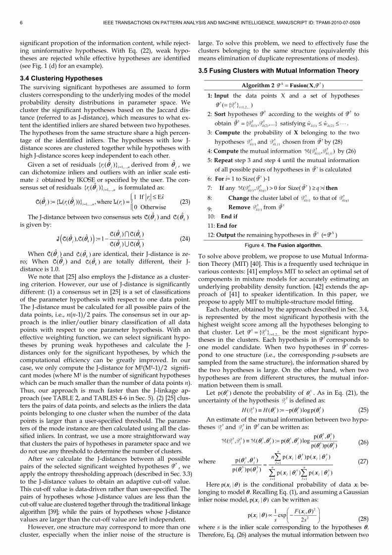
6 IEEE TRANSACTIONS ON PATTERN ANALYSIS AND MACHINE INTELLIGENCE, MANUSCRIPT ID: TPAMI-2010-07-0509
significant propotion of the information content, while reject-ing uninformative hypotheses. With Eq. (22), weak hypo-theses are rejected while effective hypotheses are identified (see Fig. 1 (d) for an example).
3.4 Clustering Hypotheses The surviving significant hypotheses are assumed to form clusters corresponding to the underlying modes of the model probability density distributions in parameter space. We cluster the significant hypotheses based on the Jaccard dis-tance (referred to as J-distance), which measures to what ex-tent the identified inliers are shared between two hypotheses. The hypotheses from the same structure share a high percen-tage of the identified inliers. The hypotheses with low J-distance scores are clustered together while hypotheses with high J-distance scores keep independent to each other.
Given a set of residuals 1,...,ˆ{ ( )}i j i nr =θ derived from ˆ
jθ , we can dichotomize inliers and outliers with an inlier scale esti-mate s obtained by IKOSE or specified by the user. The con-sensus set of residuals 1,...,
ˆ{ ( )}i j i nr =θ is formulated as:
1,...,
ˆ1 If Eˆ ˆ( ) : { ( ( ))} ,where ( )0 Otherwise
ij i j i n i
r sr r=
≤= =
θ θC L L (23)
The J-distance between two consensus sets ˆ( )jθC and ˆ( )kθC is given by:
( )ˆ ˆ( ) ( )ˆ ˆ( ), ( ) : 1ˆ ˆ( ) ( )
j kj k
j k
= −
θ θθ θ
θ θC C
J C CC C
(24)
When ˆ( )jθC and ˆ( )kθC are identical, their J-distance is ze-ro; When ˆ( )jθC and ˆ( )kθC are totally different, their J-distance is 1.0.
We note that [25] also employs the J-distance as a cluster-ing criterion. However, our use of J-distance is significantly different: (1) a consensus set in [25] is a set of classifications of the parameter hypothesis with respect to one data point. The J-distance must be calculated for all possible pairs of the data points, i.e., n(n-1)/2 pairs. The consensus set in our ap-proach is the inlier/outlier binary classification of all data points with respect to one parameter hypothesis. With an effective weighting function, we can select significant hypo-theses by pruning weak hypotheses and calculate the J-distances only for the significant hypotheses, by which the computational efficiency can be greatly improved. In our case, we only compute the J-distance for M†(M†-1)/2 signifi-cant modes (where M† is the number of significant hypotheses which can be much smaller than the number of data points n). Thus, our approach is much faster than the J-linkage ap-proach (see TABLE 2, and TABLES 4-6 in Sec. 5). (2) [25] clus-ters the pairs of data points, and selects as the inliers the data points belonging to one cluster when the number of the data points is larger than a user-specified threshold. The parame-ters of the mode instance are then calculated using all the clas-sified inliers. In contrast, we use a more straightforward way that clusters the pairs of hypotheses in parameter space and we do not use any threshold to determine the number of clusters.
After we calculate the J-distances between all possible pairs of the selected significant weighted hypotheses *P , we apply the entropy thresholding approach (described in Sec. 3.3) to the J-distance values to obtain an adaptive cut-off value. This cut-off value is data-driven rather than user-specified. The pairs of hypotheses whose J-distance values are less than the cut-off value are clustered together through the traditional linkage algorithm [39]; while the pairs of hypotheses whose J-distance values are larger than the cut-off value are left independent.
However, one structure may correspond to more than one cluster, especially when the inlier noise of the structure is
large. To solve this problem, we need to effectively fuse the clusters belonging to the same structure (equivalently this means elimination of duplicate representations of modes).
3.5 Fusing Clusters with Mutual Information Theory
Algorithm 2 †( , )Δ = Fusion XP P
1: Input the data points X and a set of hypotheses † †
1,2,...( { } )i i==P P 2: Sort hypotheses †P according to the weights of †P to
obtain † † †(1) (2){ , ,...}λ λ=P P P satisfying (1) (2)ˆ ˆw wλ λ≤ ≤ ⋅ ⋅ ⋅ .
3: Compute the probability of X belonging to the two hypotheses †
( )iλP and †( )jλP chosen from †P by (28)
4: Compute the mutual information † †( ) ( )( , )i jλ λP PM by (26)
5: Repeat step 3 and step 4 until the mutual information of all possible pairs of hypotheses in †P is calculated
6: For i= 1 to Size( †P )-1 7: If any † †
( ) ( )( , ) 0i qλ λ >P PM for Size( †P ) ≥ q >i then
8: Change the cluster label of †( )iλP to that of †
( )qλP 9: Remove †
( )iλP from †P 10: End if 11: End for 12: Output the remaining hypotheses in †P (= ΔP )
Figure 4. The Fusion algorithm.
To solve above problem, we propose to use Mutual Informa-tion Theory (MIT) [40]. This is a frequently used technique in various contexts: [41] employs MIT to select an optimal set of components in mixture models for accurately estimating an underlying probability density function. [42] extends the ap-proach of [41] to speaker identification. In this paper, we propose to apply MIT to multiple-structure model fitting.
Each cluster, obtained by the approach described in Sec. 3.4, is represented by the most significant hypothesis with the highest weight score among all the hypotheses belonging to that cluster. Let † †
1,2,...{ }i i==P P be the most significant hypo-theses in the clusters. Each hypothesis in †P corresponds to one model candidate. When two hypotheses in †P corres-pond to one structure (i.e., the corresponding p-subsets are sampled from the same structure), the information shared by the two hypotheses is large. On the other hand, when two hypotheses are from different structures, the mutual infor-mation between them is small.
Let †p( )iθ denote the probability of †iθ . As in Eq. (21), the
uncertainty of the hypothesis †iP is defined as:
† † † †( ) ( ) : p( ) log p( )i i i iH H≡ = −P θ θ θ (25)
An estimate of the mutual information between two hypo-theses †
iP and †jP in †P can be written as:
(26)
where (27)
Here p( | )l θx is the conditional probability of data xi be-longing to model θ. Recalling Eq. (1), and assuming a Gaussian inlier noise model, p( | )l θx can be written as:
(28)
where s is the inlier scale corresponding to the hypotheses θ. Therefore, Eq. (26) analyses the mutual information between two
2
2
1 ( , )p( | ) exp
2l
F
s s
∝ −
θθ xx i
† †† † † † † †
† †
p( , )( , ) ( , ) : p( , ) log
p( )p( )i j
i j i j i ji j
≡ =P Pθ θ
θ θ θ θθ θ
M M
† †† †
1† †
† †
1 1
p( | )p( | )p( , )
p( )p( ) p( | ) p( | )
n
l i l ji j l
n ni j
l i l jl l
n=
= =
=
θ θθ θθ θ θ θ
x x
x x

H. WANG ET AL.: SIMULTANEOUSLY FITTING AND SEGMENTING MULTIPLE STRUCTURE DATA WITH OUTLIERS 7
hypotheses by measuring the degree of similarity between the inlier distributions centered respectively on the two hypotheses.
When the mutual information between †iP and †
jP (i.e., † †( , )i jP PM ) is larger than zero, †iP and †
jP are statistically dependent; Otherwise, †
iP and †jP are statistically independent.
[41] employs MIT to prune mixture components in Gaussian mixture models. In contrast, we apply MIT in multiple-structure model fitting. We are pruning/fusing related descriptions of general data (e.g., identifying “similar” lines, circles, planes, homographies or a fundamental matrices - “similar” in that they “explain” the same portion of data).
The fusion algorithm is summarized in Fig. 4. The func-tion Size(⋅) returns the number of hypotheses. The weight scores of hypotheses indicate the goodness of model candi-dates. We first order the hypotheses according to their weights: from the weakest to the most significant weight. When we find a pair of hypotheses which are statistically dependent on each other, we fuse the hypothesis with a lower weight score to the hypothesis with a higher weight score.
4 THE COMPLETE ALGORITHM OF AKSWH
Algorithm 3 [ , ] ( ,K)Δ = AKSWH XP Cs
Input data points X and the K value 1: Estimate the parameter of a model hypothesis ˆ
jθ using a p-subset chosen from X
2: Derive the residual 1,...,ˆ ˆ( ) { ( )}j i j i nr =ℜ =θ θ of the data points
3: Estimate the scale ˆˆ ( ( ), K)jK js = ℜIKOSE θ
by Alg.1
4: Compute the weight of the hypothesis ˆ jw by (16) 5: Repeat step 1 to step 4 many times to obtain a set of
weighted hypotheses 1, 2 ,... 1,2 ,...
ˆ ˆ{ } {( , )}i i i i iw= == =P P θ 6: Select significant hypotheses * ⊂P ( P) from P by the
approach introduced in Sec. 3.3 7: Run the clustering procedure introduced in Sec. 3.4 on
*P to obtain clusters and select the most significant hypothesis in each cluster according to the weights of hypotheses † † *
1,2,...{ }i i== ⊂P PP 8: Fuse the hypotheses †P to obtain 1,2,...{ }i i
Δ Δ==P P by Alg. 2
9: Derive the inlier/outlier dichotomy using ΔP
10:Output the hypotheses ΔP and the inlier/outlier dicho-tomies 1,2,...{ ( )} )i i
Δ=PCs (= C corresponding to each of the
hypotheses in ΔP
Figure 5. The complete AKSWH algorithm.
With all the ingredients developed in the previous sections, we now propose the complete AKSWH algorithm: summa-rized in Fig. 5. After the estimation, one can use all the indenti-fied inliers to refine each estimated hypothesis.
Because some robust approaches such as RANSAC, MSAC, HT, RHT, MS and J-linkage require the user to spec-ify the inlier scale or the scale-related bin size or bandwidth, and also it is interesting to evaluate the effectiveness of the weighting functions in (16) and (17), we provide an alterna-tive version of AKSWH with a user-input inlier scale (here we refer to our approach with a fixed inlier scale as AKSWH1 and refer to AKSWH with the adaptive scale estimation ap-proach as AKSWH2). For AKSWH1, we input the inlier scale instead of the K value, and we do not run step 3 – instead simply passing the user supplied tolerance as the scale estimate for all hypotheses and using this to determine the (single global) bandwidth. All the remaining steps are the same as AKSWH2.
Fig. 1 and Fig. 6 respectively illustrate some results of AKSWH2 and AKSWH1 (the results are similar; essentially only the computational time taken is different) in planar ho-mography detection using “Merton College II” (referred to as “MC2”). We employ the direct linear transform (DLT) algorithm (Alg. 4.2, p.109, [43]) to compute the homography hypotheses from a set (5000 in size) of randomly chosen p-subsets (here a p-subset is 4 pairs of point correspondences in two images). For each estimated homography hypothesis, we use the symmetric transfer error model (p.94, [43]) to compute the resi-duals. For AKSWH2, there are 384 significant hypotheses selected from the 5000 hypotheses, and 19 clusters are ob-tained at the clustering step. In comparison, the number of the selected significant hypotheses and the number of clusters before the fusion step obtained by AKSWH1 are respectively 806 and 45. Although the segmentation results obtained by AKSWH1 are the same as those obtained by AKSWH2, AKSWH2 is more effective in selecting significant hypotheses due to the more effective weighting function.
For the computational time used by AKSWH2, around 74% of the whole time is used to generate 5000 hypothesis candidates from the randomly sampled p-subsets and com-pute the weights of the hypotheses (step 1 to step 5 in Fig. 5), and about 25% of the whole time is used to cluster the signif-icant hypotheses (step 7 in Fig. 5). The significant hypothesis selection (step 6) and the fusion of the clusters (step 8) take less than 1% of the whole time. In contrast, AKSWH1 uses about 26% of the computational time in generating hypothe-sis candidates and computing the weights of the hypotheses, and 73% of the whole time in clustering the significant hypo-theses (because more hypotheses are selected for clustering when the less effective weighting function is used). Thus we can see that effectively selecting significant hypotheses (step 6 in Fig. 5) will significantly affect the computational speed of AKSWH1/2. We will give more comparisons between AKSWH1/2 in Sec. 5.
(a) (b) (c)
Figure 7. Segmentation results for the “Merton College III” (referred to as “MC3”) image pair obtained by AKSWH2. (a) and (b) The input image pair with SIFT feature [1] points and corresponding matches superim-posed respectively. (c) The segmentation results. (d) to (f) The in-lier/outlier dichotomy obtained by IKOSE (corresponding to the left, mid-dle and right plane respectively).
(d) (e) (f)
Figure 6. Some results obtained by AKSWH1. (a) Over-segmented clus-ters after the clustering step using a fixed inlier scale. (b) The final ob-tained segmentation result obtained by AKSWH1.
(a) (b)

8 IEEE TRANSACTIONS ON PATTERN ANALYSIS AND MACHINE INTELLIGENCE, MANUSCRIPT ID: TPAMI-2010-07-0509
Fig. 7 shows the homography-based segmentation results obtained by AKSWH2. AKSWH2 automatically selects 268 significant hypotheses from 10000 hypotheses and correctly detects three planar homographies. Fig. 7 (d) to (f) illustrate the probability density distributions of the ordered (by the absolute residual value) correspondences for the selected model instance and the adaptive inlier/outlier dichotomy estimated by IKOSE (in AKSWH2). We can see that IKOSE has correctly detected the inlier-outlier dichotomy boundary.
5 EXPERIMENTS We compare AKSWH with RHT [8], ASKC [17, 29], MS [20, 21], RHA [24], J-linkage [25] and KF [26]. The choice of the competitors was informed by the suggestions of the review-ers and by the following reasons: (1) we choose J-linkage (which uses the Jaccard distance as a criterion to cluster data points) and ASKC (which is also developed based on kernel density estimate) because they are the most related ap-proaches to the proposed approach. (2) We choose RHT and MS because both approaches work in parameter space. (3) RHA and KF estimate the parameters of model instances si-multaneously and claim to have the ability to estimate the number of structures. Thus we also choose RHA and KF.
As indicated earlier - we test two versions of our approach: AKSWH1 with a fixed inlier scale, and AKSWH2 with an adaptive inlier scale estimate. AKSWH1 is not intended to be a proposed method – we use it only to evaluate the relative effects of the more sophisticated weighting scheme intro-duced in Sec. 3.2. Nonetheless we find that it performs re-markably well – albeit at slower speed and slightly less accu-racy, generally.
In running RHT, MS, J-linkage and AKSWH1, we manually specify the inlier scale for these approaches. We specify the number of model instances for ASKC and the minimum in-lier number (which has influence on determining the number of model instances) for RHT. MS, RHA, J-linkage and KF need some user-specified thresholds: which have significant influence on determining the estimate of the model instance number (see Sec. 1 for more detail). Thus, we adjust the thre-
shold values so that the approaches of RHT, MS, RHA, J-linkage and KF output the correct model instance number. Neither the number of model instances nor the true scale is required for AKSWH2. The value of K in AKSWH1/2 is fixed to be 10% of the whole data points for all the following expe-riments and we do not adjust any other parameter or thre-shold for AKSWH2 (note: we specify the inlier scale for AKSWH1 for comparison purpose only).
Although there are other sampling techniques (e.g., [33, 34]), we employ random sampling for all the approaches, because: (1) it is easy to implement and it does not require extra thresholds (e.g., the threshold in the exponent function in [25], or the matching scores in [33, 34]); (2) It is the most widely used approach to generate hypothesis candidates.
To measure the fitting errors, we first find the correspond-ing relationship between the estimated model instances and the true model instances (for real data/image, we manually obtain the true parameters of model instances and the true inliers to the model instance). Then, we fit the true inliers to the corresponding model instances estimated by the ap-proaches, and fit the classified inliers by the approaches to the true parameters of the corresponding model instances. For RHT, MS, RHA, J-linkage and AKSWH1, the inliers be-longing to a model instance are classified using the given ground truth inlier scale while for ASKC, KF and AKSWH2, the inlier scales are adaptively estimated. There are 5000 p-subsets generated for each dataset used in Sec. 5.1, Sec. 5.2.1 to Sec. 5.2.3, 10000 p-subsets for each dataset used in Sec. 5.2.4, and 20000 for each dataset used in Sec. 5.2.5.
5.1 Simulations with Synthetic Data We evaluate the eight approaches on line fitting using four
sets of synthetic data (see Fig. 8). The residuals are calculated by the standard regression definition. We compare the fitting error results and the computational speed2 (TABLE 2). From Fig. 8 and TABLE 2, we can see that for the three-line data, AKSWH1/2 succeed in fitting and segmenting the three lines
2 For MS, we use the C++ code from http://coewww.rutgers.edu/riul,, For J-linkage, we use the Matlab code from http://www.toldo.info.
(a) Data (b) RHT (c) MS (d) RHA (e) J-linkage (f) KF (g) AKSWH2 Figure 8. Examples for line fitting and segmentation. 1st to 4th rows respectively fit three, four, five and six lines. The corresponding outlier percentages are respectively 85%, 85%, 87% and 90%. The inlier scale is 1.5. (a) The original data with a total number of 1000 in eachdataset, are distributed in the range of [0, 100]. (b) to (g) The results obtained by RHT, MS, RHA, J-linkage, KF and AKSWH2, respectively. We do not show the results of AKSWH1 and ASKC which are similar to those of AKSWH2 due to the space limit.

H. WANG ET AL.: SIMULTANEOUSLY FITTING AND SEGMENTING MULTIPLE STRUCTURE DATA WITH OUTLIERS 9
automatically. With some user-adjusted thresholds, RHT, ASKC, J-linkage and KF also correctly fit all the three lines: RHT and ASKC achieves lightly higher fitting errors than AKSCH1/2, while KF achieves the lowest fitting error among the eight methods because the gross outliers are effectively removed at the first step. However, AKSWH2 is much faster than KF and J-linkage (about 40 times faster than KF and 5.5 times faster than J-linkage). AKSWH2 is faster than AKSWH1 (about 3.4 times faster) because AKSWH2 uses a more effective weight-ing function, resulting in less selected significant hypotheses (376 significant hypotheses) than AKSWH1 (1682 selected significant hypotheses). RHT is faster (but has larger fitting error) than AKSWH2 because RHT uses several additional user-specified thresholds: which are used to stop the random sampling procedure. MS and RHA respectively fit one/two lines but fail to fit the other lines.
TABLE 2 THE FITTING ERRORS IN PARAMETER ESTIMATION (AND THE CPU
TIME IN SECONDS).
M1 M2 M3 M4 M5 M6 M7 M8
3 lines 1.28
(0.80) 1.21
(6.72) 23.7
(7.56) 25.1
(8.12) 1.17
(25.2) 0.99 (177)
1.18 (15.4)
1.13(4.52)
4 lines 13.3 (0.84)
1.16 (8.10)
24.2 (5.87)
48.5 (7.31)
8.67 (19.5)
1.06 (223)
1.16(17.7)
1.12(4.02)
5 lines 19.9 (0.79)
1.40 (8.46)
7.35 (7.26)
116 (7.86)
10.9 (23.7)
9.27 (116)
1.25(14.2)
1.29(4.12)
6 lines 15.7 (1.21)
1.21 (11.0)
47.0 (5.53)
178 (9.06)
27.6 (23.2)
1.20 (685)
1.17(20.2)
1.15(3.43)
(M1-RHT; M2-ASKC; M3-MS; M4-RHA; M5-J-LINKAGE; M6-KF; M7-AKSWH1; M8-AKSWH2. WE RUN THE APPAROACHES ON A LAPTOP WITH
AN I7 2.66GHZ CPU IN WINDOW 7 PLATFORM)
For the four line data, AKSWH1/2, ASKC and KF correctly fit the four lines. However, AKSWH2 is significant faster than KF and ASKC. In contrast, RHT and J-linkage correctly fit three lines but wrongly fit one. MS and RHA correctly fit two/one lines but fail to fit two/three, respectively.
For the five line data, only AKSWH1/2 and ASKC correct-
ly fit all five lines, while ASKC achieves relatively higher fit-ting error than AKSWH1/2. J-linkage and KF correctly fit four of the five lines, while RHT and RHA fit three lines but wrongly fit two. MS only fits two lines correctly.
In fitting the six lines, AKSWH1/2, ASKC and KF correctly fit the six lines. We note that KF costs much higher CPU time in fitting the six-line data than the three-line data (around 4 times slower). This is because KF obtains more clusters (30 clusters) for the six-line data than the three-line data (20 clus-ters) at the step of spectral clustering, and most of the CPU time is spent on merging clusters in the step of model selec-tion. ASKC also uses more CPU time in fitting to the six-line data than the three-line data. In contrast, AKSWH2 uses com-parable CPU time for both types of data and is about 200 times faster than KF and more than 3 times faster than ASKC.
TABLE 3 THE FITTING ERRORS IN PARAMETER ESTIMATION.
Inlier scale Outlier percentage Cardinality ratio
Std.Var. Max.Err. Std.Var. Max.Err. Std.Var. Max.Err.RHT 4.75 36.1 0.36 31.2 2.90 26.7
ASKC 0.06 3.01 0.10 6.23 2.30 18.5 MS 5.03 46.3 7.70 49.6 3.85 32.8
RHA 19.3 333 27.0 334 14.3 143 J-linkage 5.60 41.0 2.06 45.6 5.95 22.6
KF 0.19 8.14 0.11 6.41 1.07 20.4 AKSWH1 0.04 2.88 0.09 6.01 0.02 0.86 AKSWH2 0.06 2.75 0.09 6.09 0.03 0.86
We also evaluate the performance of the eight approaches in different inlier scales, outlier percentages, and the cardi-nality ratios of inliers belonging to each model instance. For the following experiment, we use the three-line data similar to that used in Fig. 9. Changes in inlier scales: we generate the three line data with 80% outlier percentage. The inlier scale of each line is slowly increased from 0.1 to 3.0. Changes in outlier percentages: we draw the breakdown plot to test the influence of outlier percentage on the performance of the
(a) (b) RHT (c) ASKC (d) MS (e) RHA (f) J-linkage (g) KF (h) AKSWH2
Figure 10. Examples for line fitting with real images. 1st (“tennis court”) and 2th (“tracks”) rows respectively fit six and seven lines. (a) The original im-ages; (b) to (g) are the results obtained by RHT, ASKC, MS, RHA, J-linkage, KF and AKSWH2, respectively. We do not show the results obtained byAKSWH1, which are very similar to those of AKSWH2, due to the space limit.
Figure 9. The average results obtained by the eight approaches. (a-c) respectively shows the influence of inlier scale, outlier percentage, and therelative cardinality radio of outliers to inliers.
(a) (b) (c)
Legend

10 IEEE TRANSACTIONS ON PATTERN ANALYSIS AND MACHINE INTELLIGENCE, MANUSCRIPT ID: TPAMI-2010-07-0509
eight approaches. We gradually decrease the inlier number of each line equally while we increase the number of the ran-domly distributed outliers. The inlier scale of each line is set to 1.0. Changes in cardinality ratios between the inliers of each line: The inlier numbers of the three lines are equal to each other at the beginning and the inlier scales of all lines are 1.0. We gradually reduce the inlier number of one line while we increase the number of data points belonging to the other lines. Thus, the relative cardinality ratio between the lines is increased gradually. We repeat the experiment twenty times and we report both the average results (in Fig. 9), and the averaged standard variances and the worst results (in TABLE 3) of the fitting errors.
As shown in Fig. 9 and TABLE 3, AKSWH1/2 show ro-bustness to the influence of the inlier scale, the outlier per-centage and the inlier cardinality ratio, and both achieve the most accurate results among the competing approaches. In contrast, RHA does not achieve good results for all the three experiments. MS does not work well for the experiments in Fig. 9 (b) and (c) but it works reasonably well in Fig. 9 (a) when the inlier scale is less than 0.3. Among the four ap-proaches: RHT, ASKC, J-linkage and KF, in Fig. 9 (a) RHT and J-linkage respectively break down when the inlier scale is larger than 1.4 and 0.8; in contrast, ASKC and KF achieve relatively good performance when ASKC is given the num-ber of model instances and the step-size in KF is adjusted manually. In Fig. 9 (b), it shows that J-linkage and RHT begin to break down when the outlier percentage is larger than 84% and 89% respectively, and both achieve better results than MS and RHA but worse results than ASKC and KF. In Fig. 9 (c), it shows that ASKC and KF work well when the relative cardinality ratio of inliers is small but they begin to break down when the inlier cardinality ratio is larger than 2.0 and 2.2 respectively. J-linkage and RHT achieve worse re-sults than ASKC and KF.
It is worth noting that when we fix the step-size h to be 50 (as specified in Fig. 2 in [26]), KF wrongly estimates the number of model instances in about 10% of the experiments
in Fig. 9 (a), 2.3% in Fig. 9 (b) and 52.3% in Fig. 9 (c). When the inlier cardinality ratio of model instances in Fig. 9 (c) is larger than 2.3, KF wrongly estimates almost all the number of model instances in the experiments. In contrast AKSWH2 with a fixed K value correctly find the model instance number for all the experiments in Fig. 9.
5.2 Experiments with Real Images3
5.2.1 Line Fitting We test the performance of the eight approaches using real images for line fitting (shown in Fig. 10). For the “tennis court” image which includes six lines, there are 4160 edge points detected by the Canny operator [44]. As KF consumes a large memory resource in calculating the kernel matrix and in spectral clustering, we randomly resample 2000 data points for “tennis court” and test KF on the resampled data. As shown in Fig. 10 and TABLE 4, AKSWH1/2 and J-linkage correctly fit all the six lines. However, AKSWH1/2 are much faster than J-linkage and KF (AKSWH1/2 are respectively 12/25 and 208/426 times faster than J-linkage and KF). Among the other competing approaches, MS fits two lines but fails in fitting four lines; RHT, ASKC and KF succeed in fitting five out of the six lines while RHA correctly fit four lines only. We note that ASKC fits two estimated lines to the same real line and so does KF (as pointed by the green arrows in Fig. 10). While this does not occur to AKSWH1/2 because it uses MIT to effectively fuse over-clustered modes belonging to the same model instance.
For the “tracks” image which includes seven lines, 1022 Canny edge points are detected. Only KF and AKSWH1/2 successfully fit all the seven lines in this challenging case. ASKWH2 (4.23 seconds) is about 40 times faster than KF and
3 To make the readers easy to test and compare their approaches with the competing approaches in this paper, we put the data used in the paper (for line fitting, circle fitting, homography based segmentation and fundamental matrix based segmentation) and the corresponding ground truth (for homo-graphy based segmentation and fundamental matrix based segmentation) online: http://cs.adelaide.edu.au/~dsuter/code_and_data/
(a) (b) RHT (c) ASKC (d) MS (e) RHA (f) J-linkage (g) KF (h) AKSWH2
Figure 12. Examples for range image segmentation. 1st (“five planes” including 10842 data points) to 2th (“block” having 12069 data points) rows fit five
planes. (a) The original images; (b) to (g) The segmentation results obtained by RHT, ASKC, MS, RHA, J-linkage, KF and AKSWH2, respectively.
(a) (b) RHT (c) ASKC (d) MS (e) RHA (f) J-linkage (g) KF (h) AKSWH2
Figure 11. Examples for circle fitting. 1st (“cups”) to 2th (“coins”) rows respectively fit four and six circles. (a) The original images; (b) to (h) The
results obtained by RHT, ASKC, MS, RHA, J-linkage, KF and AKSWH2, respectively.
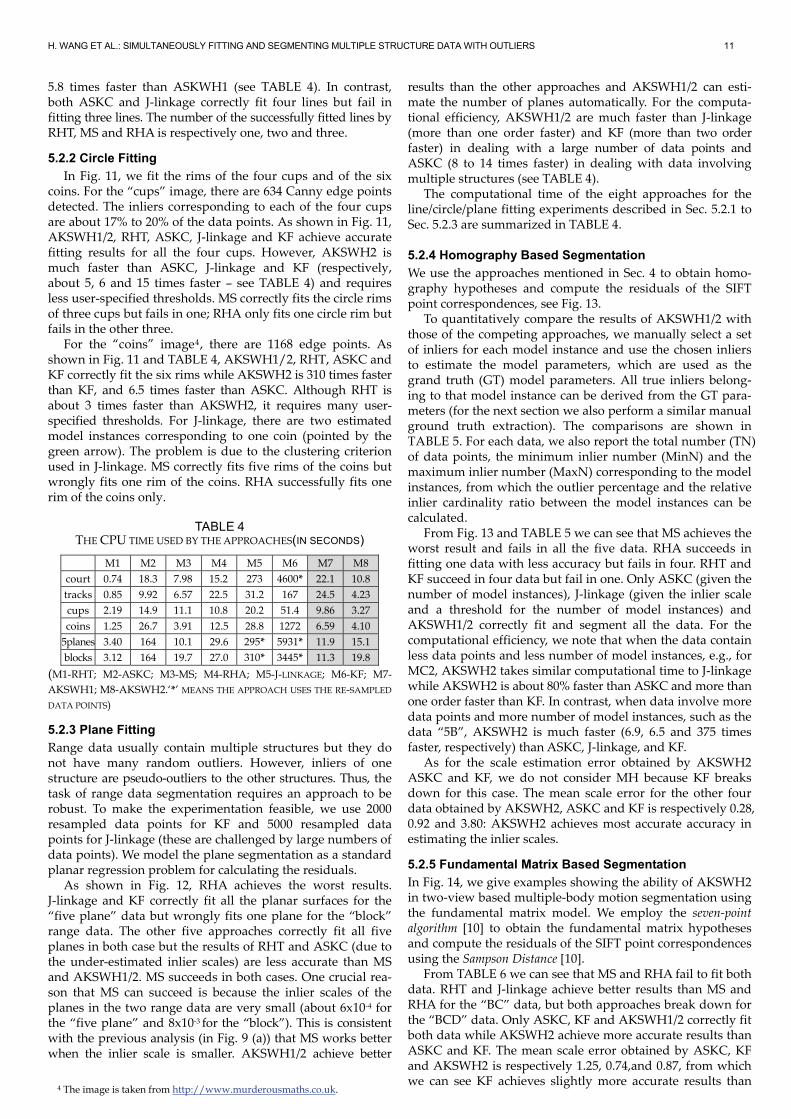
H. WANG ET AL.: SIMULTANEOUSLY FITTING AND SEGMENTING MULTIPLE STRUCTURE DATA WITH OUTLIERS 11
5.8 times faster than ASKWH1 (see TABLE 4). In contrast, both ASKC and J-linkage correctly fit four lines but fail in fitting three lines. The number of the successfully fitted lines by RHT, MS and RHA is respectively one, two and three.
5.2.2 Circle Fitting
In Fig. 11, we fit the rims of the four cups and of the six coins. For the “cups” image, there are 634 Canny edge points detected. The inliers corresponding to each of the four cups are about 17% to 20% of the data points. As shown in Fig. 11, AKSWH1/2, RHT, ASKC, J-linkage and KF achieve accurate fitting results for all the four cups. However, AKSWH2 is much faster than ASKC, J-linkage and KF (respectively, about 5, 6 and 15 times faster – see TABLE 4) and requires less user-specified thresholds. MS correctly fits the circle rims of three cups but fails in one; RHA only fits one circle rim but fails in the other three.
For the “coins” image4, there are 1168 edge points. As shown in Fig. 11 and TABLE 4, AKSWH1/2, RHT, ASKC and KF correctly fit the six rims while AKSWH2 is 310 times faster than KF, and 6.5 times faster than ASKC. Although RHT is about 3 times faster than AKSWH2, it requires many user-specified thresholds. For J-linkage, there are two estimated model instances corresponding to one coin (pointed by the green arrow). The problem is due to the clustering criterion used in J-linkage. MS correctly fits five rims of the coins but wrongly fits one rim of the coins. RHA successfully fits one rim of the coins only.
TABLE 4 THE CPU TIME USED BY THE APPROACHES(IN SECONDS)
M1 M2 M3 M4 M5 M6 M7 M8court 0.74 18.3 7.98 15.2 273 4600* 22.1 10.8tracks 0.85 9.92 6.57 22.5 31.2 167 24.5 4.23cups 2.19 14.9 11.1 10.8 20.2 51.4 9.86 3.27coins 1.25 26.7 3.91 12.5 28.8 1272 6.59 4.10
5planes 3.40 164 10.1 29.6 295* 5931* 11.9 15.1blocks 3.12 164 19.7 27.0 310* 3445* 11.3 19.8
(M1-RHT; M2-ASKC; M3-MS; M4-RHA; M5-J-LINKAGE; M6-KF; M7-AKSWH1; M8-AKSWH2.‘*’ MEANS THE APPROACH USES THE RE-SAMPLED
DATA POINTS)
5.2.3 Plane Fitting
Range data usually contain multiple structures but they do not have many random outliers. However, inliers of one structure are pseudo-outliers to the other structures. Thus, the task of range data segmentation requires an approach to be robust. To make the experimentation feasible, we use 2000 resampled data points for KF and 5000 resampled data points for J-linkage (these are challenged by large numbers of data points). We model the plane segmentation as a standard planar regression problem for calculating the residuals.
As shown in Fig. 12, RHA achieves the worst results. J-linkage and KF correctly fit all the planar surfaces for the “five plane” data but wrongly fits one plane for the “block” range data. The other five approaches correctly fit all five planes in both case but the results of RHT and ASKC (due to the under-estimated inlier scales) are less accurate than MS and AKSWH1/2. MS succeeds in both cases. One crucial rea-son that MS can succeed is because the inlier scales of the planes in the two range data are very small (about 6x10⁻⁴ for the “five plane” and 8x10⁻³ for the “block”). This is consistent with the previous analysis (in Fig. 9 (a)) that MS works better when the inlier scale is smaller. AKSWH1/2 achieve better
4 The image is taken from http://www.murderousmaths.co.uk.
results than the other approaches and AKSWH1/2 can esti-mate the number of planes automatically. For the computa-tional efficiency, AKSWH1/2 are much faster than J-linkage (more than one order faster) and KF (more than two order faster) in dealing with a large number of data points and ASKC (8 to 14 times faster) in dealing with data involving multiple structures (see TABLE 4).
The computational time of the eight approaches for the line/circle/plane fitting experiments described in Sec. 5.2.1 to Sec. 5.2.3 are summarized in TABLE 4.
5.2.4 Homography Based Segmentation
We use the approaches mentioned in Sec. 4 to obtain homo-graphy hypotheses and compute the residuals of the SIFT point correspondences, see Fig. 13.
To quantitatively compare the results of AKSWH1/2 with those of the competing approaches, we manually select a set of inliers for each model instance and use the chosen inliers to estimate the model parameters, which are used as the grand truth (GT) model parameters. All true inliers belong-ing to that model instance can be derived from the GT para-meters (for the next section we also perform a similar manual ground truth extraction). The comparisons are shown in TABLE 5. For each data, we also report the total number (TN) of data points, the minimum inlier number (MinN) and the maximum inlier number (MaxN) corresponding to the model instances, from which the outlier percentage and the relative inlier cardinality ratio between the model instances can be calculated.
From Fig. 13 and TABLE 5 we can see that MS achieves the worst result and fails in all the five data. RHA succeeds in fitting one data with less accuracy but fails in four. RHT and KF succeed in four data but fail in one. Only ASKC (given the number of model instances), J-linkage (given the inlier scale and a threshold for the number of model instances) and AKSWH1/2 correctly fit and segment all the data. For the computational efficiency, we note that when the data contain less data points and less number of model instances, e.g., for MC2, AKSWH2 takes similar computational time to J-linkage while AKSWH2 is about 80% faster than ASKC and more than one order faster than KF. In contrast, when data involve more data points and more number of model instances, such as the data “5B”, AKSWH2 is much faster (6.9, 6.5 and 375 times faster, respectively) than ASKC, J-linkage, and KF.
As for the scale estimation error obtained by AKSWH2 ASKC and KF, we do not consider MH because KF breaks down for this case. The mean scale error for the other four data obtained by AKSWH2, ASKC and KF is respectively 0.28, 0.92 and 3.80: AKSWH2 achieves most accurate accuracy in estimating the inlier scales.
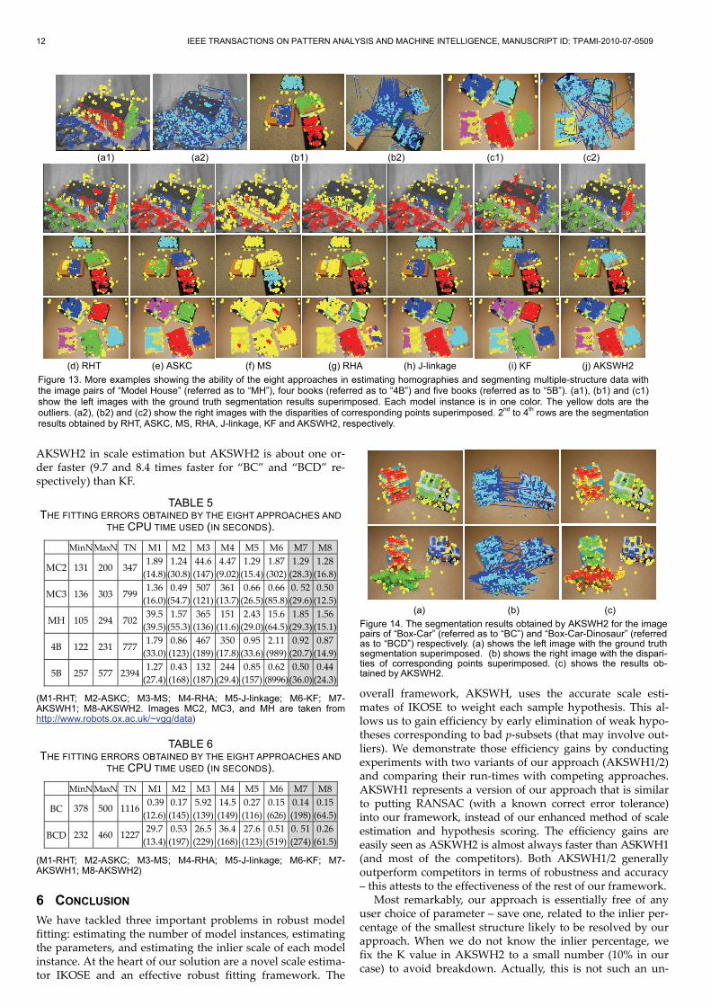
5.2.5 Fundamental Matrix Based Segmentation
In Fig. 14, we give examples showing the ability of AKSWH2 in two-view based multiple-body motion segmentation using the fundamental matrix model. We employ the seven-point algorithm [10] to obtain the fundamental matrix hypotheses and compute the residuals of the SIFT point correspondences using the Sampson Distance [10].
From TABLE 6 we can see that MS and RHA fail to fit both data. RHT and J-linkage achieve better results than MS and RHA for the “BC” data, but both approaches break down for the “BCD” data. Only ASKC, KF and AKSWH1/2 correctly fit both data while AKSWH2 achieve more accurate results than ASKC and KF. The mean scale error obtained by ASKC, KF and AKSWH2 is respectively 1.25, 0.74,and 0.87, from which we can see KF achieves slightly more accurate results than
12 IEEE TRANSACTIONS ON PATTERN ANALYSIS AND MACHINE INTELLIGENCE, MANUSCRIPT ID: TPAMI-2010-07-0509
AKSWH2 in scale estimation but AKSWH2 is about one or-der faster (9.7 and 8.4 times faster for “BC” and “BCD” re-spectively) than KF.
TABLE 5 THE FITTING ERRORS OBTAINED BY THE EIGHT APPROACHES AND
THE CPU TIME USED (IN SECONDS).
MinN MaxN TN M1 M2 M3 M4 M5 M6 M7 M8
MC2 131 200 347 1.89
(14.8) 1.24
(30.8) 44.6(147)
4.47 (9.02)
1.29 (15.4)
1.87 (302)
1.29(28.3)
1.28(16.8)
MC3 136 303 799 1.36
(16.0) 0.49
(54.7) 507
(121)361
(13.7) 0.66
(26.5) 0.66
(85.8) 0. 52(29.6)
0.50(12.5)
MH 105 294 702 39.5
(39.5) 1.57
(55.3) 365
(136)151
(11.6) 2.43
(29.0) 15.6
(64.5) 1.85
(29.3)1.56
(15.1)
4B 122 231 777 1.79
(33.0) 0.86 (123)
467(189)
350 (17.8)
0.95 (33.6)
2.11 (989)
0.92(20.7)
0.87(14.9)
5B 257 577 2394 1.27
(27.4) 0.43 (168)
132(187)
244 (29.4)
0.85 (157)
0.62 (8996)
0.50(36.0)
0.44(24.3)
(M1-RHT; M2-ASKC; M3-MS; M4-RHA; M5-J-linkage; M6-KF; M7-AKSWH1; M8-AKSWH2. Images MC2, MC3, and MH are taken from http://www.robots.ox.ac.uk/~vgg/data)
TABLE 6 THE FITTING ERRORS OBTAINED BY THE EIGHT APPROACHES AND
THE CPU TIME USED (IN SECONDS).
MinN MaxN TN M1 M2 M3 M4 M5 M6 M7 M8
BC 378 500 1116 0.39 (12.6)
0.17 (145)
5.92(139)
14.5 (149)
0.27 (116)
0.15 (626)
0.14(198)
0.15(64.5)
BCD 232 460 1227 29.7 (13.4)
0.53 (197)
26.5 (229)
36.4 (168)
27.6 (123)
0.51 (519)
0. 51(274)
0.26(61.5)
(M1-RHT; M2-ASKC; M3-MS; M4-RHA; M5-J-linkage; M6-KF; M7-AKSWH1; M8-AKSWH2)
6 CONCLUSION We have tackled three important problems in robust model fitting: estimating the number of model instances, estimating the parameters, and estimating the inlier scale of each model instance. At the heart of our solution are a novel scale estima-tor IKOSE and an effective robust fitting framework. The
overall framework, AKSWH, uses the accurate scale esti-mates of IKOSE to weight each sample hypothesis. This al-lows us to gain efficiency by early elimination of weak hypo-theses corresponding to bad p-subsets (that may involve out-liers). We demonstrate those efficiency gains by conducting experiments with two variants of our approach (AKSWH1/2) and comparing their run-times with competing approaches. AKSWH1 represents a version of our approach that is similar to putting RANSAC (with a known correct error tolerance) into our framework, instead of our enhanced method of scale estimation and hypothesis scoring. The efficiency gains are easily seen as ASKWH2 is almost always faster than ASKWH1 (and most of the competitors). Both AKSWH1/2 generally outperform competitors in terms of robustness and accuracy – this attests to the effectiveness of the rest of our framework.
Most remarkably, our approach is essentially free of any user choice of parameter – save one, related to the inlier per-centage of the smallest structure likely to be resolved by our approach. When we do not know the inlier percentage, we fix the K value in AKSWH2 to a small number (10% in our case) to avoid breakdown. Actually, this is not such an un-
(a1) (a2) (b1) (b2) (c1) (c2)
(d) RHT (e) ASKC (f) MS (g) RHA (h) J-linkage (i) KF (j) AKSWH2
Figure 13. More examples showing the ability of the eight approaches in estimating homographies and segmenting multiple-structure data withthe image pairs of “Model House” (referred as to “MH”), four books (referred as to “4B”) and five books (referred as to “5B”). (a1), (b1) and (c1)show the left images with the ground truth segmentation results superimposed. Each model instance is in one color. The yellow dots are theoutliers. (a2), (b2) and (c2) show the right images with the disparities of corresponding points superimposed. 2nd to 4th rows are the segmentationresults obtained by RHT, ASKC, MS, RHA, J-linkage, KF and AKSWH2, respectively.
(a) (b) (c)
Figure 14. The segmentation results obtained by AKSWH2 for the imagepairs of “Box-Car” (referred as to “BC”) and “Box-Car-Dinosaur” (referredas to “BCD”) respectively. (a) shows the left image with the ground truthsegmentation superimposed. (b) shows the right image with the dispari-ties of corresponding points superimposed. (c) shows the results ob-tained by AKSWH2.

H. WANG ET AL.: SIMULTANEOUSLY FITTING AND SEGMENTING MULTIPLE STRUCTURE DATA WITH OUTLIERS 13
usual assumption as the inlier percentage estimate has been usually either assumed known, or fixed to some low value, and then used to determine the number of the required p-subsets in many robust approaches which employ the popular ran-dom sampling scheme. We acknowledge that in some cases (probably most) the user does not know the outlier percen-tage in any reasonably accurate or precise form. This issue is related to the issue of “how big should the recovered popula-tions/structures be”. This issue is compounded by other as-pects related to structural scale (e.g., how close two planes are in fitting, for example, planar parts of a wall with small recesses, etc.). As stated in Sec. 1, we do not claim that we have proposed an automatic system which has solved all the problems of recovery of structure from image data: this is impossible because how many structures there are in a scene is usually a question without a unique answer. However, the number of structures can be determined when we assume that all the structures of interest are relatively large and have roughly comparable size (we ignore the structures with very few sup-porting data points). In our approach, such an assumption is implicit by using a conservative K (in this paper, we fix the K value to be 10% of the data points for all the experiments). This can be thought of as (roughly) saying we are assuming we are not interested in finer scale structure that makes up less than 10% of the data points. Our experiments show that the proposed method, whilst having no claims of optimality, is effective. Of course, our approach is not without some drawbacks and possible improvements. For example, guided sampling approaches may improve the efficiency. Likewise, though we have demonstrated superiority to the comparator methods, as described in their published forms, that does not preclude improvements to those approaches. Finally, it also must be acknowledged that one is not always strictly com-paring apples with apples and oranges with oranges. For example, many techniques in this area were developed under the assumption there is a dominant single structure – and thus were never explicitly designed to recover multiple struc-tures, though perhaps others have tried to extend the me-thods to do so by fit-and-remove iterations etc. When one has only a single dominant structure, or perhaps knows the scale of noise, other methods still suffice. However, our method still generally performs well – albeit slower.
Compared to the more recent methods of ASKC [17, 29], J-Linkage [25] and KF [26], the advantage of our method can be understood as such: ASKC is not developed for multi-structure fitting, thus it may suffer from the problems related to sequential fit-and-remove. J-Linkage requires a user-given global inlier threshold (which may be difficult to determine), thus it assumes similar noise scales across all structures. Fi-nally, as our experiments show, KF does not tolerate very well different inlier population sizes. In contrast, for reasons already described above (i.e., accurate scale estimator, paral-lel fitting via hypothesis weighting and fusion), AKSWH is significantly more tolerant to the issues faced by the other methods.
ACKNOWLEDGEMENTS
The authors would like to thank the reviewers for their valu-able comments, which greatly helped to improve the paper. Parts of our code are developed based on the “Structure and Motion Toolkit” provided by Prof. P. Torr. We also thank Dr. R. Toldo and Prof. A. Fusiello for sharing the code of J-linkage, and Dr. R. Subbarao and Prof. P. Meer for sharing the code of MS. We thank Prof. A. Bab-Hadiashar for provid-ing some range image data. This work was supported by the
Australian Research Council (ARC) under the project DP0878801, by the National Natural Science Foundation of China under project 61170179 and by the Xiamen Science & Technology Planning Project Fund (3502Z20116005) of China. Most of this work was completed when the first author was at the University of Adelaide.
REFERENCES
1. Lowe, D.G., Distinctive Image Features from Scale-Invariant Keypoints. International Journal of Computer Vision, 2004. 60(2). 91-110.
2. Wang, H., D. Suter, Robust Adaptive-Scale Parametric Model Estimation for Computer Vision. IEEE Trans. Pattern Analysis and Machine Intelli-gence, 2004. 26(11). 1459-1474.
3. Stewart, C.V., Bias in Robust Estimation Caused by Discontinuities and Multiple Structures. IEEE Trans. Pattern Analysis and Machine Intelli-gence, 1997. 19(8). 818-833.
4. Huber, P.J., Robust Statistics. New York, Wiley, 1981. 5. Rousseeuw, P.J., Least Median of Squares Regression. Journal of the
American Statistical Association, 1984. 79. 871-880. 6. Rousseeuw, P.J., A. Leroy, Robust Regression and outlier detection. John
Wiley & Sons, New York., 1987. 7. Hough, P.V.C., Methods and means for recognising complex patterns, in
U.S. Patent 3 069 654. 1962. 8. XU, L., E. OJA, P. KULTANEN, A New Curve Detection Method: Rando-
mized Hough Transform (RHT). Pattern Recognition Letters, 1990. 11(5). 331-338.
9. Fischler, M.A., R.C. Bolles, Random Sample Consensus: A Paradigm for Model Fitting with Applications to Image Analysis and Automated Carto-graphy. Commun. ACM, 1981. 24(6). 381-395.
10. Torr, P., D. Murray, The Development and Comparison of Robust Methods for Estimating the Fundamental Matrix. International Journal of Computer Vision, 1997. 24(3). 271-300.
11. Miller, J.V., C.V. Stewart. MUSE: Robust Surface Fitting Using Unbiased Scale Estimates. IEEE Computer Vision and Pattern Recognition. 1996. 300-306.
12. Stewart, C.V., MINPRAN: A New Robust Estimator for Computer Vision. IEEE Trans. Pattern Analysis and Machine Intelligence, 1995. 17(10). 925-938.
13. Lee, K.-M., P. Meer, R.-H. Park, Robust Adaptive Segmentation of Range Images. IEEE Trans. Pattern Analysis and Machine Intelligence, 1998. 20(2). 200-205.
14. Yu, X., T.D. Bui, A. Krzyzak, Robust Estimation for Range Image Segmen-tation and Reconstruction. IEEE Trans. Pattern Analysis and Machine Intel-ligence, 1994. 16(5). 530-538.
15. Chen, H., P. Meer. Robust Regression with Projection Based M-estimators. IEEE International Conference on Computer Vision. 2003. 878-885.
16. Hoseinnezhad, R., A. Bab-Hadiashar. A Novel High Breakdown M-estimator for Visual Data Segmentation. International Conference on Com-puter Vision. 1997. 1-6.
17. Wang, H., D. Mirota, M. Ishii, et al. Robust Motion Estimation and Struc-ture Recovery from Endoscopic Image Sequences With an Adaptive Scale Kernel Consensus Estimator IEEE Computer Vision and Pattern Recogni-tion. 2008.
18. Zuliani, M., C.S. Kenney, B.S. Manjunath. The multiRANSAC Algorithm and Its Application to Detect Planar Homographies. IEEE International Conference on Image Processing. 2005. 153-156.
19. Vidal, R., Y. Ma, S. Sastry, Generalized principal component analysis (GPCA). IEEE Trans. Pattern Analysis and Machine Intelligence, 2004. 27(12). 1945-1959.
20. Fukunaga, K., L.D. Hostetler, The Estimation of the Gradient of a Density Function, with Applications in Pattern Recognition. IEEE Trans. Info. Theory, 1975. IT-21. 32-40.
21. Comaniciu, D., P. Meer, Mean Shift: A Robust Approach towards Feature Space A Analysis. IEEE Trans. Pattern Analysis and Machine Intelligence, 2002. 24(5). 603-619.
22. Tuzel, O., R. Subbarao, P. Meer. Simultaneous Multiple 3D Motion Estima-tion via Mode Finding on Lie Groups. IEEE International Conference on Computer Vision. 2005. 18-25.
23. Subbarao, R., P. Meer, Nonlinear Mean Shift over Riemannian Manifolds. International Journal on Computer Vision, 2009. 84(1). 1-20.
24. Zhang, W., J. Kosecka, Nonparametric Estimation of Multiple Structures with Outliers. LNCS, DVW, 2006. 4358. 60-74.
25. Toldo, R., A. Fusiello. Robust Multiple Structures Estimation with J-Linkage. European Conference on Computer Vision. 2008. 537-547.
26. Chin, T.-J., H. Wang, D. Suter. Robust Fitting of Multiple Structures: The Statistical Learning Approach. IEEE International Conference on Comput-er Vision. 2009. 413-420.
27. Weiss, Y., E.H. Adelson. A Unified Mixture Framework for Motion Seg-mentation: Incorporating Spatial Coherence and Estimating the Number of

14 IEEE TRANSACTIONS ON PATTERN ANALYSIS AND MACHINE INTELLIGENCE, MANUSCRIPT ID: TPAMI-2010-07-0509
Models. Proceedings of IEEE conference on Computer Vision and Pattern Recognition. 1996. 321-326.
28. Kanatani, K., C. Matsunaga. Estimating the Number of Independent Mo-tions for Multibody Motion Segmentation. Asian Conference on Computer Vision 2002. 7-12.
29. Wang, H., D. Mirota, G. Hager, A Generalized Kernel Consensus Based Robust Estimator. IEEE Transactions on Pattern Analysis and Machine In-telligence, 2010. 32(1). 178-184.
30. Wang, H., D. Suter. Robust Fitting by Adaptive-Scale Residual Consensus. 8th European Conference on Computer Vision. 2004. 107-118.
31. Bab-Hadiashar, A., D. Suter, Robust segmentation of visual data using ranked unbiased scale estimate. ROBOTICA, International Journal of In-formation, Education and Research in Robotics and Artificial Intelligence, 1999. 17. 649-660.
32. Torr, P., A. Zisserman, MLESAC: A New Robust Estimator With Applica-tion to Estimating Image Geometry. Computer Vision and Image Under-standing, 2000. 78(1). 138-156.
33. Tordoff, B., D.W. Murray, Guided Sampling and Consensus for Motion Estimation. European Conference on Computer Vision, 2002. 82-96.
34. Chum, O., J. Matas. Matching with PROSAC: Progressive Sample Consen-sus. IEEE Computer Vision and Pattern Recognition. 2005. 220-226.
35. Wand, M.P., M. Jones, Kernel Smoothing. Chapman & Hall, 1995. 36. Silverman, B.W., Density Estimation for Statistics and Data Analysis. 1986,
London: Chapman and Hall. 37. Sezgin, M., B. Sankur, Survey Over Image Thresholding Techniques and
Quantitative Performance Evaluation. Journal of Electronic Imaging, 2004. 13(1). 146-165.
38. Ferraz, L., R. Felip, B. Martínez, et al. A Density-Based Data Reduction Algorithm for Robust Estimators. Lecture Notes in Computer Science. 2007. 355-362.
39. Duda, R.O., P.E. Hart, Pattern Classification and Scene Analysis. 1973: John Wiley and Sons.
40. Shannon, C.E., The Mathematical Theory of Communication. Bell Systems Technique Journal, 1948. 27. 379-423.
41. Yang, Z.R., M. Zwolinski, Mutual Information Theory for Adaptive Mixture Models. IEEE Transactions on Pattern Analysis and Machine Intelligence, 2001. 23(4). 396-403.
42. Lee, Y., K.Y. Lee, J. Lee, The Estimating Optimal Number of Gaussian Mixtures Based on Incremental k-means for Speaker Identification. Interna-tional Journal of Information Technology, 2006. 12(7). 13-21.
43. Hartley, R., A. Zisserman, Multiple View Geometry in Computer Vision. 2nd ed. 2004: Cambridge University Press.
44. Canny, J.F., A Computational Approach to Edge Detection. IEEE Transac-tions on Pattern Analysis and Machine Intelligence, 1986. 8. 679-697.
Hanzi Wang is currently a Distin-guished Professor and “Minjiang Scho-lar” at Xiamen University, China, and an Adjunct Professor at the University of Adelaide, Australia. He was a Senior Research Fellow (2008-2010) at the University of Adelaide, Australia; an Assistant Research Scientist (2007-2008) and a Postdoctoral Fellow (2006-2007) at the Johns Hopkins University;
and a Research Fellow at Monash University, Australia (2004-2006). He received the Ph.D degree in Computer Vision from Monash University, Australia. He was awarded the Douglas Lampard Electrical Engineering Research Prize and Medal for the best PhD thesis in the Department. His research interests are concentrated on computer vision and pattern recognition includ-ing visual tracking, robust statistics, model fitting, object detec-tion, video segmentation, and related fields. He has published around 50 papers in major international journals and confe-rences including the IEEE Transactions on Pattern Analysis and Machine Intelligence, International Journal of Computer Vision, ICCV, CVPR, ECCV, NIPS, MICCAI, etc. He is an Associate Editor for IEEE Transactions on Circuits and Systems for Video Technology (T-CSVT) and he was a Guest Editor of Pattern Recognition Letters (September 2009). He is a Senior Member of the IEEE. He has served as a reviewer for more than 30 jour-nals and conferences.
Tat-Jun Chin received a B.Eng. in Mechatronics Engineering from Un-iversiti Teknologi Malaysia (UTM) in 2003, and subsequently in 2007 a Ph.D. in Computer Systems Engineering from Monash University, Victoria, Australia. He was a Research Fellow at the Insti-tute for Infocomm Research in Singa-pore from 2007-2008. Since 2008 he is a Lecturer at The University of Ade-laide, Australia. His research interests
include robust estimation and statistical learning methods in Computer Vision.
David Suter received a B.Sc.degree in applied mathematics and physics (The Flinders University of South Australia 1977), a Grad. Dip. Comp. (Royal Mel-bourne Institute of Technology 1984)), and a Ph.D. in computer science (La Trobe University, 1991). He was a Lec-turer at La Trobe from 1988 to 1991; and a Senior Lecturer (1992), Associate
Professor (2001), and Professor (2006-2008) at Monash Univer-sity, Melbourne, Australia. Since 2008 he has been a professor in the school of Computer Science, The University of Adelaide. He is head of the School of Computer Science. He served on the Australian Research Council (ARC) College of Experts from 2008-2010. He is on the editorial boards of International Journal of Computer Vision. He has previously served on the editorial boards of Machine Vision and Applications and the Internation-al Journal of Image and Graphics. He was General co-Chair or the Asian Conference on Computer Vision (Melbourne 2002) and is currently co-Chair of the IEEE International Conference on Image Processing (ICIP2013).