Simultaneous prediction of four ATP­binding cassette transporters' substrates using multi­label QSAR

Article (Accepted Version)

http://sro.sussex.ac.uk

Aniceto, Natália, Freitas, Alex, Bender, Andreas and Ghafourian, Taravat (2016) Simultaneous prediction of four ATP-binding cassette transporters' substrates using multi-label QSAR. Molecular Informatics, 35 (10). pp. 514-528. ISSN 1868-1743

This version is available from Sussex Research Online: http://sro.sussex.ac.uk/id/eprint/64121/

This document is made available in accordance with publisher policies and may differ from the published version or from the version of record. If you wish to cite this item you are advised to consult the publisher’s version. Please see the URL above for details on accessing the published version.

Copyright and reuse: Sussex Research Online is a digital repository of the research output of the University.

Copyright and all moral rights to the version of the paper presented here belong to the individual author(s) and/or other copyright owners. To the extent reasonable and practicable, the material made available in SRO has been checked for eligibility before being made available.

Copies of full text items generally can be reproduced, displayed or performed and given to third parties in any format or medium for personal research or study, educational, or not-for-profit purposes without prior permission or charge, provided that the authors, title and full bibliographic details are credited, a hyperlink and/or URL is given for the original metadata page and the content is not changed in any way.

1

DOI: 10.1002/minf.200

Simultaneous prediction of four ATP-binding cassette transporters substrates using multi-label QSAR

Natália Aniceto[a]

, Alex Freitas[b]

, Andreas Bender[c]

, Taravat Ghafourian[a,d]*

1 Introduction

The drug development process is becoming increasingly

more expensive over the years, which is partly caused by

stricter testing demanded by regulatory entities for a drug to

be accepted into the market. At the same time the reduction

of animal experimentation has become a priority. As a result

in silico programs in the pharmaceutical industry play an

increasingly important role in drug discovery for the financial

sustainability of a company.

The ATP-binding cassette (ABC) family is composed (in

humans) of 48 exclusive membrane exporters that are

grouped in seven families (ABCA-G) according to gene

similarity with respect to sequence and organization. They

transport a wide variety of endogenous and exogenous

compounds, which range from ions to macromolecules, via

an ATP-dependent mechanism.[1-2]

These transporters are

highly expressed in a variety of tissues, among which are

some important distribution barriers that are associated with

drug absorption and distribution impairment. Some

examples are the intestinal brush border membrane, the

blood-brain barrier, and the hepatocytic biliary canalicular

membrane.[3]

The role of membrane transporters in absorption, distribution and excretion as well as the possible

drug interaction due to binding to these transporters indicate

the importance of membrane transporters to drug discovery

and development, where about 1/3 of the attrition rate in

drug development is caused by a poor pharmacokinetic

profile.[4]

Something as simple as a high hepatic clearance

can render the use of a highly active, non-toxic drug

unfeasible due to the need for very short dosage periods.

Properties like this are often not discovered until human

trials, which means that any drug withdrawals are extremely

expensive for the company. In silico studies are a promising

and inexpensive tool to avoid or at least minimize late drug

attrition rate. Among these, quantitative structure-activity (or

property) relationships (QSAR) have long been

implemented in the drug discovery and development

process.

Given the high potential of ABC transporters for

pharmacoketic impact and also their potential for drug-drug

interaction, these membrane transporters are one of the

most important targets that need to be studied during drug

discovery. In addition, some ABC transporters including the

Breast Cancer Resistance Protein (BCRP1, ABCG2), P-

glycoprotein (P-gp, MDR1, ABCB1), and the Multidrug

Resistance-associated Proteins (MRP1-7, ABCC1-6 and

10)[1]

are strongly associated with multi-drug resistance in

cancer cells given their ability to extrude drugs from the

cell.[2]

QSAR appears to be a particularly well suited method

to predict ABC transport substrates since it has been shown

that substrate recognition by the aforementioned ABC

members relies on global physicochemical profiles rather

than following the key-and-lock ligand binding model.[2]

The

potential of QSAR to predict ABC transporter substrates

during the R&D process has already been demonstrated by

Desai et al.[5]

who reported the successful replacement of an

in vitro automated assay with a QSAR model to predict P-gp

substrates in an early stage of the drug development

pipeline of Eli Lilly. Currently, improving the accuracy of

QSARs to predict (classify) substrates and non-substrates

of ABC transporters remains a challenge. This is partly due

to the multi-specific nature of the substrate recognition by

these transporters. Different ABC family members have

shown redundancy in terms of substrate recognition and

transport,[2, 6]

and in order to take advantage of this, we

suggest a multi-label QSAR approach to address the ABC

transport as a whole, as opposed to the traditional single-

label QSAR approach looking at each transporter

individually.

Keywords: Multi-label Classification, QSAR, transporter, P-glycoprotein, Multidrug-resistance Associated Protein, Breast Cancer Resistance

protein, BCRP1, MRP1, MRP2

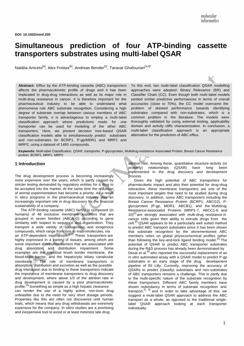
Abstract: Efflux by the ATP-binding cassette (ABC) transporters

affects the pharmacokinetic profile of drugs and it has been

implicated in drug-drug interactions as well as its major role in

multi-drug resistance in cancer. It is therefore important for the

pharmaceutical industry to be able to understand what

phenomena rule ABC substrate recognition. Considering a high

degree of substrate overlap between various members of ABC

transporter family, it is advantageous to employ a multi-label

classification approach where predictions made for one

transporter can be used for modeling of the other ABC

transporters. Here, we present decision tree-based QSAR

classification models able to simultaneously predict substrates

and non-substrates for BCRP1, P-gp/MDR1 and MRP1 and

MRP2, using a dataset of 1493 compounds.

To this end, two multi-label classification QSAR modelling

approaches were adopted: Binary Relevance (BR) and

Classifier Chain (CC). Even though both multi-label models

yielded similar predictive performances in terms of overall

accuracies (close to 70%), the CC model overcame the

problem of skewed

substrates compared

common problem in

performance towards identifying

with non-substrates, which is a

the literature. The models were

thoroughly validated by using external testing, applicability

domain and activity cliffs characterization. In conclusion, a

multi-label classification approach is an appropriate

alternative for the prediction of ABC efflux.

2

In traditional supervised learning, among n training

instances (compounds in the dataset), each instance

(compound) is assumed to be associated with a single

response (called label). In other words, in a single-label

classifier, each compound is classed under one label

(response), e.g. active or inactive. So for each response

(label), a different classifier is produced which is independent

from the classifier produced for other labels.[7]

However, there are cases where instances, due to their

complexity, might have various simultaneous responses,

which is the same as saying that an instance is associated

to a set of various labels rather than just one. This is the

case of the ABC transport problem, where different

compounds are effluxed by different types of ABC

transporters, and it constitutes a multi-label classification

problem. So, in this scenario, the machine learning

algorithm produces a multi-label classifier, which can be

viewed as a set of single-label classification models, one per

label (response).[7-8]

However, one of the big issues in multi-label machine learning is that labels can have interdependency between

them[8]

. Correlation between labels potentially holds important information about the modelled problem, and

accounting for this is crucial in facilitating the learning

algorithm[9]

. As a result, the main goal in multi-label machine learning is to enable the detection of these relationships.

This means that the considerable overlap between

substrates (and inhibitors) of various ABC transporters

should be exploited from the data mining standpoint to

improve the model performance.

Within multi-label classification techniques, one of the

most widely used problem transformation methods is Binary

Relevance (BR), which decomposes the multi-label problem

into a binary problem for each label separately. A regular

single-label classifier is then applied to predict the 0/1 class

in every separate label ignoring the information from the

remaining labels. The separate predictions from all the

single-label classification tasks are finally gathered in one

multi-label prediction.[8, 10]

Consequently, BR has a major drawback by assuming label independence. By separating

the labels one is in fact losing potentially useful information

and it leads to a situation like predicting impossible

coexisting labels in practice.[8, 10]

An alternative to this is the classifier chain (CC) method that is able to address label

dependency.[10]

In this technique, the different labels originating from single-label models communicate the

learned information to each other, in a sequential fashion.

A multi-label approach has recently been applied to classify inhibitors/non-inhibitors of two transporters, P-gp

and BCRP1 [11]

, although the authors reported no value in accounting for label overlap for the inhibitors of these two

proteins. Here, we have focused instead on the

substrates/non substrates of four major ABC transporters,

namely BCRP1, MDR1/P-gp, MRP1, MRP2, using novel

multi-label classification methods. The goal was to assess

the potential value of taking into account the data overlap

amongst transporters in terms of the predictive accuracy of

the classifier, as well as finding molecular characteristics

that are unique to, or those that overlap between the

substrates of various transporters. The two previously

mentioned multi-label modelling schemes, BR and CC, were

employed where the only difference between them is the

absence or presence of communication between transporter

models, respectively. A comprehensive validation routine

including the characterization of the applicability domain

(AD) and activity cliffs (AC) were carried out for the models.

The predictive performance was analyzed against each

model’s applicability domain and activity cliff analysis, in the

attempt of providing a more holistic, in-depth interpretation

of the models’ true worth. To our knowledge this is the first

reported multi-label classification model for the prediction of

ABC substrates (S) and non-substrates (NS), providing

insight on transporter relationship with regard to binding

patterns.

2 Experimental Section

2.1 Dataset

A dataset of 1493 compounds was compiled from the

substrate data available on the Metrabase database[12]

(accessed on October 2014) for six ABC transporters:

BCRP1, MDR1, MRP1, MRP2, MRP3 and MRP4. All

instances were divided into two classes: substrates and non-

substrates. The collection of SMILES provided was checked

for repetitions and isomers using ACD Labs, and mixtures

were removed. Repetitions were merged and, for cases of

conflicting information, the principle of minimum evidence

was applied, by which all compounds with at least one case

of reported substrate property were regarded as potential

substrates and so, they were classified as substrates. This is

a valid approach considering that all the

initial data collected from Metrabase was selected based on

quality standards.[12]

Prior to any modelling or modelling-related task the dataset

was submitted to a stratification procedure as described by

Sechidis et al.[13]

. The authors show that this procedure

leads to data subsets with more balanced class label

distributions in a series of benchmark datasets. That is, this

procedure maximizes transporters distribution across

different data partitions. This procedure was implemented in

R using the provided pseudo-code. Consequently, the

dataset was divided into training (TR), internal validation (IV)

and test (TE) set in a proportion of 6:2:2 (895 + 299 + 299

compounds), respectively, with similar distribution of

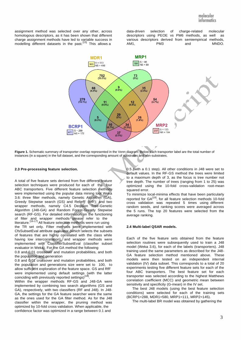
substrates and non-substrates in TR, IV and TE. For larger

datasets, i.e. BCRP1, MDR1, MRP1 and MRP2 compounds,

there was only a negligible imbalance of data with the

substrate (S) to non-substrate (NS) ratio of 1.7, 1.3, 1.0 and

1.2, respectively (see Figure 1). However, for the transporter

classes associated with smaller datasets, namely MRP3

and MRP4, the S to NS ratio was around 2.5, which led to

insufficient number of non-substrates for modelling and

validation. Therefore, these two transporters were

eliminated and the remaining four transporters were

investigated.

2.2 Calculation of Molecular Descriptors.

Molecular descriptors were calculated using ACD/labs logD

suite v12.5 and MOE 2013, using the SMILES codes

retrieved from Metrabase. Using ACD, prior to molecular

descriptors calculation, all structures were submitted to

desalting. In MOE, the compounds’ structures were washed

(counter ions were removed) and minimized. Molecular

mechanics minimization was initially performed using

MMFF94x, followed by a second minimization using

quantum mechanics Self-Consistent Field (SCF), where

partial charges were assigned using the PM6 Hamiltonian.

The PM6 semi-empirical method was added to MOE as a

MOPAC 2009[14]

extension. After descriptor calculation, all external, non-variant and mainly zero-valued descriptors

(with ≥97% zero values) were removed. No single charge-

3

assignment method was selected over any other, across

homologous descriptors, as it has been shown that different

charge assignment methods have led to variable success in

modelling different datasets in the past.[15]

This allows a

data-driven selection of charge-related molecular

descriptors using PEOE vs PM6 methods, as well as

various descriptors derived from semiempirical methods,

AM1, PM3 and MNDO.

Figure 1. Schematic summary of transporter overlap represented in the Venn diagram. Below each transporter label are the total number of instances (in a square) in the full dataset, and the corresponding amount of substrates and non-substrates.

2.3 Pre-processing feature selection.

A total of five feature sets derived from five different feature

selection techniques were produced for each of the four

ABC transporters. Five different feature selection methods

were implemented using the popular data mining tool Weka

3.6: three filter methods, namely Genetic Algorithm (GA),

Greedy Stepwise search (GS) and ReliefF (RfF); and two

wrapper methods, namely C4.5 Decision Tree-Genetic

Algorithm (J48-GA) and Random Forest-Greedy Stepwise

search (RF-GS). For detailed information on the functioning

of filter and wrapper methods please refer to the

literature.[16-17]

All feature selection methods were run using

the TR set only. Filter methods were implemented with

CfsSubsetEval attribute evaluator (which selects the subsets

of features that are highly correlated with the class while

having low intercorrelation), and wrapper methods were

implemented with ClassifierSubsetEval (classifier subset

evaluator in Weka). For the GA method the following

0.8 and 0.01 crossover and mutation probabilities, and both

the population and generation

0.8 and 0.01 crossover and mutation probabilities, and both

the population and generations size were set to 100, to

allow sufficient exploration of the feature space. GS and RfF

were implemented using default settings (with the latter

coinciding with previously reported settings)[18]

.

Within the wrapper methods RF-GS and J48-GA were

implemented by combining two search algorithms (GS and

GA), respectively, with two classifiers (RF and J48). In J48-

GA, the settings for the GA feature searcher were the same

as the ones used for the GA filter method. As for the J48

classifier within the wrapper, the pruning method was

optimized by 10-fold cross validation. When applicable, the

confidence factor was optimized in a range between 0.1 and

0.5 (with a 0.1 step). All other conditions in J48 were set to

default values. In the RF-GS method the trees were limited

to a maximum depth of 3, as the focus is tree number not

tree depth. The number of trees (ranging from 1 to 25) was

optimized using the 10-fold cross-validation root-mean

squared error.

To minimize local-minima effects that have been particularly

reported for GA[19]

, for all feature selection methods 10-fold cross validation was repeated 5 times using different

random seeds, and ranking scores were averaged across

the 5 runs. The top 20 features were selected from the

average ranking.

2.4 Multi-label QSAR models.

Each of the five feature sets obtained from the feature

selection routines were subsequently used to train a J48

model (Weka 3.6), for each of the labels (transporters). J48

training used the same parameters as described for the J48-

GA feature selection method mentioned above. These

models were then tested on an independent internal

validation (IV) data subset. This corresponds to a total of 20

experiments testing five different feature sets for each of the

four ABC transporters. The best feature set for each

transporter was selected according to the highest Matthews

correlation coefficient (MCC) and geometric mean between

sensitivity and specificity (G-mean) in the IV set.

The best J48 models (using the best feature selection

conditions) were selected for each of the training sets

(BCRP1=288, MDR1=580, MRP1=111, MRP2=145).

The multi-label BR model was obtained by gathering the

4

𝑇𝑃 + 𝐹𝑁 × 𝑇𝑁 + 𝐹𝑃 × 𝑇𝑃 + 𝐹𝑃 × 𝑇𝑁 + 𝐹𝑁

1

𝐿

multi-label CC model each label (transporter) in the 4-label

chain uses the best descriptor set previously optimized for

the BR model. In addition, as it can be seen in Figure 2,

each label in the CC model uses prediction sets from

previously available labels. In summary, in the CC model

every label (transporter) in the chain is trained using the

prediction sets from all previous labels, along with a set of

molecular descriptors (previously selected). To illustrate

this, label #3 for example, will be trained with a set of

molecular descriptors as well as class predictions for label

predictions from these four best single-label models into one

global prediction output. In this case, whenever a new query

compound needs to be predicted it would be passed

through all four ABC models and a set of label predictions

would be produced. For the multi-label CC model, the

schematic representation of CC is depicted in Figure 2. The

transporters were ordered according to descending order of

dataset size, based on the theoretical expectation that larger

datasets will have a better chance of providing useful

information to smaller datasets than the other way around.

Accordingly, the order of the labels in the classifier chain

was P-gp/MDR1 > BCRP1 > MRP2 > MRP1. To build the

𝑀𝐶𝐶 =

𝑆𝐸𝑁 = 𝑇𝑃

𝑇𝑃 + 𝐹𝑁

𝑆𝑃𝐸 = 𝑇𝑁

𝑇𝑁 + 𝐹𝑃

𝑇𝑃×𝑇𝑁 − 𝐹𝑃×𝐹𝑁

𝐺 − 𝑚𝑒𝑎𝑛 = 𝑆𝐸𝑁×𝑆𝑃𝐸

#1 and #2

Several multi-label predictive accuracy measures

were used, namely the harmonic mean between

precision and recall (F1), Precision (P) and Recall (R),

calculated according to Tsoumakas and Katakis [21-22]

.

Hamming Loss (HL) was used solely to monitor the

impact of each label on the multi-label model’s

performance, during model building.

𝐻𝑎𝑚𝑚𝑖𝑛𝑔 𝐿𝑜𝑠𝑠 = 1

𝑁

>

;?@

𝑌;∆𝑍;

𝐿

𝐹1 = 1

𝑁

>

;?@

2 𝑌; ∩ 𝑍;

𝑍; + 𝑌;

𝑃 = 1

𝑁

>

;?@

𝑌; ∩ 𝑍;

𝑍;

Figure 2. Schematic representation of multi-label classifier chain training.

Overall each transporter was submitted to an independent

𝑅 = 1

𝑁

>

;?@

𝑌; ∩ 𝑍;

𝑌;

and parallel process of feature selection, model optimization

and training, and finally testing. All these steps were

performed in parallel on the same datasets for CC and BR

in order to: 1) allow comparability between both types of

model at every level, and 2) assess the value of addressing

the overlap in the data, by fixing all other conditions in both

modelling workflows. Throughout the paper the following

notation <single-label model> - <multi-label model> will be

used whenever a specific single-label model within the CC

or the BR models is mentioned.

2.5 Model validation The single-label performance

measures used for single-label model assessment are

defined below [20]

, where TP, TN, FP and FN stand for

the numbers of true positives, true negatives, false

positives and false negatives, respectively. These

correspond to Sensitivity (SEN), specificity (SPE), Matthew’s

correlation coefficient (MCC), and the

In these measures, Yi and Zi correspond to the set of

observed and predicted labels, respectively, for the i-th

compound, N corresponds to the number of compounds in

the dataset, and L corresponds to the number of modelled

labels. The Δ symbol denotes the symmetric difference

between two sets of label values (observed and predicted,

in this case), which is equivalent to the XOR boolean

operation.

As substrates are more frequent than non-substrates in

all labels, a balanced accuracy (bACC) was used to take

into account this when assessing predictive performance,

which consisted of the average G-mean across every label j

(which, in turn, can be considered as the single-label

balanced accuracy). To evaluate the balance between

substrate and non-substrate performances across

instances, ΔPR measures the average deviation in precision

and recall between substrates and non-substrates.

G

geometric mean between SEN and SPE (G-mean). 𝑏𝐴𝐶𝐶 = 𝑆𝐸𝑁 ×𝑆𝑃𝐸 F F

F?@

5

𝑃H − 𝑃>H + 𝑅H − 𝑅>H

∆𝑃𝑅 = 2

threshold has been reported as a sensible value above

which compounds are visibly similar.[28-30]

2.6 Applicability Domain

For any QSAR model, it is necessary to define the domain

of applicability to ensure its reliability in the prediction of

properties of external compounds. In this study, the

applicability domain (AD) of all the single label models used

in the generation of multi-label BR and CC models were

characterized. To determine the AD, the distance to the

model based on the standard deviation (STD) of the

predicted values (or labels) from the ensemble of various

models was used, as this has been shown to be the most

successful method in quantifying predictive reliability across

chemical space in the data.[23-27]

This technique capitalizes

on the concept that the disparity between predictions

computed from a group of models (ensemble) is a direct

consequence of prediction reliability. A small standard

deviation will equate to highly reliable predictions, whereas

a larger value signals unreliable predictions. It has been

demonstrated that the disagreement between models leads

to a better separation between reliable and unreliable

predictions compared to traditional structure-based

measures.[27]

In this work, J48 models were developed for 10 random

samples of training set data, each sample comprising 80%

of the training set compounds.

2.8 Visualization of chemical space

3 Results

3.1 Multi-label QSAR models

In this work, the main goal was to model four ABC

𝑦 − 𝑦 L transporters in such a way that allows accounting for

𝑆𝑇𝐷 = K

𝑁 − 1

possible underlying correlations between labels ( i.e.

transporters). Multi-label classification is the appropriate

approach to achieve this. By comparing a multi-label

method that takes into account label interaction (i.e., CC)

STD values were calculated for each compound using the equation above. Here, 𝑦K is the class label prediction

using model m and 𝑦 is the average of all prediction outputs

for this compound by N models. For classification models

(which is the case here) predictions y take the form of

probabilities. By setting increasingly larger STD thresholds

(with increments of 0.05), which can also be perceived as

increasing distance to the model’s reliability core, more

compounds become included in the model. By performing

this kind of scanning through the model’s space, one is able

to establish a profile of reliability as a function of STD. In this

case we used % correct predictions, the so-called accuracy

as our measure of reliability.

2.7 Activity cliffs

To search for possible activity cliffs, the similarities between all pairs of compounds were calculated using the well-known Tanimoto coefficient (Tc) applied on 1024 bit Morgan circular fingerprints (equivalent to the extended connectivity fingerprints [ECFP], calculated using the RDkit module in python), for a radius of 2.Following the criteria for activity

cliffs used by several authors[28-30]

, we defined as an activity cliff any substance that has a different class than the majority

class of the 3 nearest training neighbors, which must all

show a Tc > 0.55 to the analyzed compound. This

with an alternative method that assumes labels to be

independent (i.e. BR) one is able determine whether label

interaction, in fact, exists. Both multi-label classifiers were

trained using the best features selected by various feature

selection methods for each transporter, and they differ only

in the use of previous label predictions as additional

features (in the case of CC). The rational for the use of multi-

label methods was the overlap observed in the dataset as

can be seen from the results of the Chi-squared test

measuring the correlations between labels (Table 1). These

multi-label methods were compared in terms of their

predictive ability in the classification of various ABC

transporters’ substrates and non-substrates.

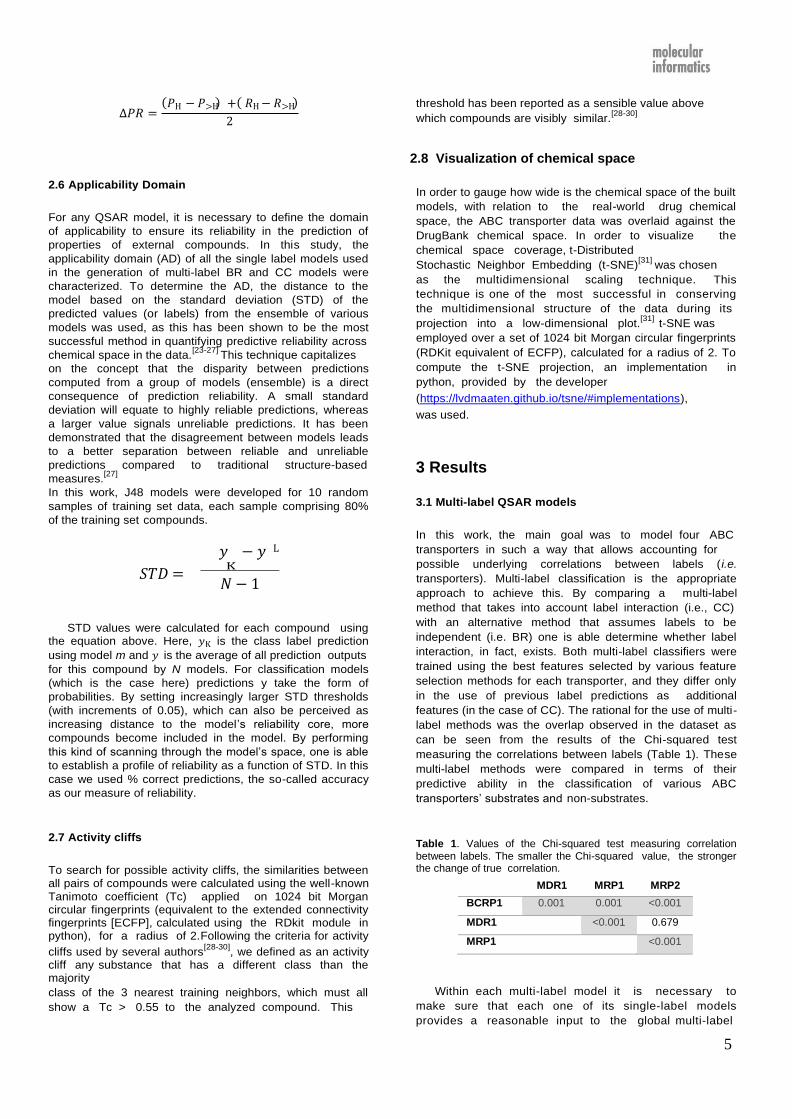
Table 1. Values of the Chi-squared test measuring correlation between labels. The smaller the Chi-squared value, the stronger the change of true correlation.

MDR1 MRP1 MRP2

BCRP1 0.001 0.001 <0.001

MDR1 <0.001 0.679

MRP1 <0.001

Within each multi-label model it is necessary to

make sure that each one of its single-label models

provides a reasonable input to the global multi-label

In order to gauge how wide is the chemical space of the built

models, with relation to the real-world drug chemical

space, the ABC transporter data was overlaid against the

DrugBank chemical space. In order to visualize the

chemical space coverage, t-Distributed

Stochastic Neighbor Embedding (t-SNE)[31]

was chosen

as the multidimensional scaling technique. This

technique is one of the most successful in conserving

the multidimensional structure of the data during its

projection into a low-dimensional plot.[31]

t-SNE was

employed over a set of 1024 bit Morgan circular fingerprints

(RDKit equivalent of ECFP), calculated for a radius of 2. To

compute the t-SNE projection, an implementation in

python, provided by the developer

(https://lvdmaaten.github.io/tsne/#implementations),

was used.

6

model. Firstly, we selected the best single-label J48

model for each transporter out of a pool of five models

obtained from various pre-processing feature selection

methods. The results showed that the GS method led to

the best model for BCPR1, while J48-GA led to the best

models for MDR1 and MRP1; and ReliefF led to the

best model for MRP2 (Supporting Information SI 1).

Table 2 shows the performance of the best single-label

models.

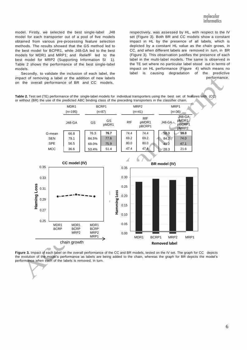
Secondly, to validate the inclusion of each label, the

impact of removing a label or the addition of new labels

on the overall performance of BR and CC models,

respectively, was assessed by HL, with respect to the IV

set (Figure 3). Both BR and CC models show a constant

impact in HL by the presence of all labels, which is

depicted by a constant HL value as the chain grows, in

CC, and when different labels are removed in turn, in BR

(Figure 3). This observation justifies the presence of each

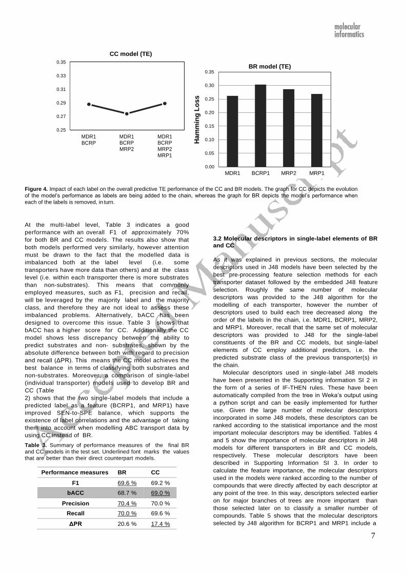
label in the multi-label models. The same is observed in

the TE set where no particular label stood out in terms of

impact on HL performance (Figure 4) which means no

label is causing degradation of the predictive

performance.

Table 2. Test set (TE) performance of the single-label models for individual transporters using the best set of features with (CC)

or without (BR) the use of the predicted ABC binding class of the preceding transporters in the classifier chain.

MDR1 BCRP1 MRP2 MRP1

(n=195) (n=87) (n=41) (n=36)

J48-GA GS

GS pMDR1

RfF

RfF pMDR1 pBCRP1

J48-GA

J48-GA pMDR1 pBCRP1 pMRP2

CC model (IV) 0.35

0.35 BR model (IV)

0.33

0.31

0.29

0.27

0.25

MDR1 BCRP

MDR1 BCRP MRP2

MDR1 BCRP MRP2 MRP1

0.30

0.25

0.20

0.15

0.10

0.05

0.00

MDR1 BCRP1 MRP2 MRP1

chain growth Removed label

Figure 3. Impact of each label on the overall performance of the CC and BR models, tested on the IV set. The graph for CC depicts

the evolution of the model’s performance as labels are being added to the chain, whereas the graph for BR depicts the model’s

performance when each of the labels is removed, in turn.

58.9

84.2

41.2

28.3

59.0

74.0

47.1

21.6

74.4 74.4

69.2 69.2

80.0 80.0

47.4 47.4

76.3

84.5%

69.0%

53.4%

76.7

77.6

75.9

51.4

G-mean 66.8

SEN 79.1

SPE 56.5

MCC 36.6

Ham

ing

Lo

ss

Ham

min

g Lo

ss

7

Ham

min

g L

oss

0.35

0.33

0.31

0.29

0.27

0.25

MDR1 BCRP

CC model (TE)

MDR1 BCRP MRP2

MDR1 BCRP MRP2 MRP1

0.35

0.30

0.25

0.20

0.15

0.10

0.05

BR model (TE)

0.00

MDR1 BCRP1 MRP2 MRP1

Figure 4. Impact of each label on the overall predictive TE performance of the CC and BR models. The graph for CC depicts the evolution

of the model’s performance as labels are being added to the chain, whereas the graph for BR depicts the model’s performance when

each of the labels is removed, in turn.

At the multi-label level, Table 3 indicates a good

performance with an overall F1 of approximately 70%

for both BR and CC models. The results also show that

both models performed very similarly, however attention

must be drawn to the fact that the modelled data is

imbalanced both at the label level (i.e. some

transporters have more data than others) and at the class

level (i.e. within each transporter there is more substrates

than non-substrates). This means that commonly

employed measures, such as F1, precision and recall,

will be leveraged by the majority label and the majority

class, and therefore they are not ideal to assess these

imbalanced problems. Alternatively, bACC has been

designed to overcome this issue. Table 3 shows that

bACC has a higher score for CC. Additionally the CC

model shows less discrepancy between the ability to

predict substrates and non- substrates, shown by the

absolute difference between both with regard to precision

and recall (ΔPR). This means the CC model achieves the

best balance in terms of classifying both substrates and

non-substrates. Moreover, a comparison of single-label

(individual transporter) models used to develop BR and

CC (Table

2) shows that the two single-label models that include a

predicted label as a feature (BCRP1, and MRP1) have

improved SEN-to-SPE balance, which supports the

existence of label correlations and the advantage of taking

them into account when modelling ABC transport data by

using CC instead of BR.

Table 3. Summary of performance measures of the final BR

and CC models in the test set. Underlined font marks the values

that are better than their direct counterpart models.

3.2 Molecular descriptors in single-label elements of BR

and CC

As it was explained in previous sections, the molecular

descriptors used in J48 models have been selected by the

best pre-processing feature selection methods for each

transporter dataset followed by the embedded J48 feature

selection. Roughly the same number of molecular

descriptors was provided to the J48 algorithm for the

modelling of each transporter, however the number of

descriptors used to build each tree decreased along the

order of the labels in the chain, i.e. MDR1, BCRP1, MRP2,

and MRP1. Moreover, recall that the same set of molecular

descriptors was provided to J48 for the single-label

constituents of the BR and CC models, but single-label

elements of CC employ additional predictors, i.e. the

predicted substrate class of the previous transporter(s) in

the chain.

Molecular descriptors used in single-label J48 models

have been presented in the Supporting information SI 2 in

the form of a series of IF-THEN rules. These have been

automatically compiled from the tree in Weka’s output using

a python script and can be easily implemented for further

use. Given the large number of molecular descriptors

incorporated in some J48 models, these descriptors can be

ranked according to the statistical importance and the most

important molecular descriptors may be identified. Tables 4

and 5 show the importance of molecular descriptors in J48

models for different transporters in BR and CC models,

respectively. These molecular descriptors have been

described in Supporting Information SI 3. In order to

calculate the feature importance, the molecular descriptors

used in the models were ranked according to the number of

compounds that were directly affected by each descriptor at

any point of the tree. In this way, descriptors selected earlier

on for major branches of trees are more important than

those selected later on to classify a smaller number of

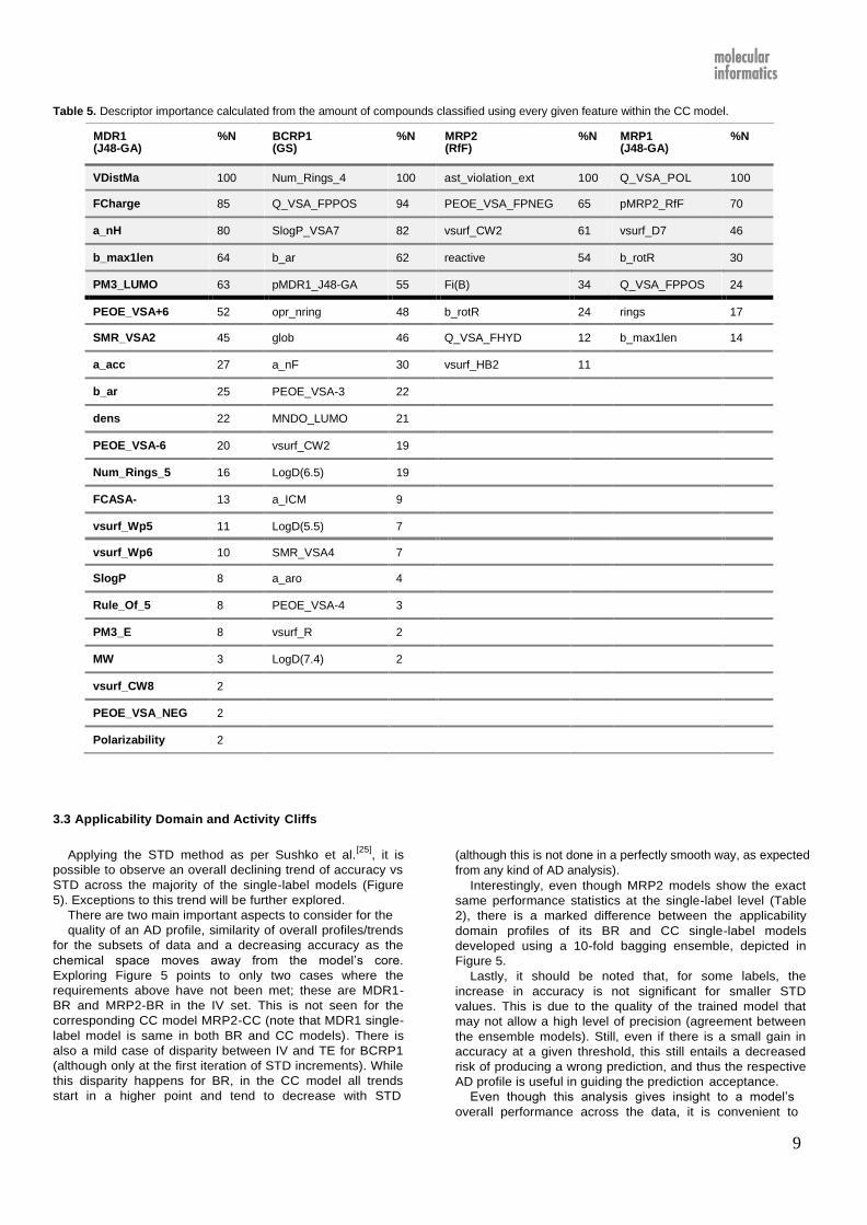
compounds. Table 5 shows that the molecular descriptors

selected by J48 algorithm for BCRP1 and MRP1 include a

Ham

min

g L

oss

Performance measures BR CC

F1 69.6 % 69.2 %

bACC 68.7 % 69.0 %

Precision 70.4 % 70.0 %

Recall 70.0 % 69.6 %

ΔPR 20.6 % 17.4 %

8

transporter substrate class predicted by the previous

transporters in the chain, and both predicted labels used in

both models affected more than 50% of the training data

(see Table 5).

Due to the design of the CC model that placed MDR1

model as the first label, the single-label MDR1 model used

in both multi-label BR and CC models is the same, i.e. no

predicted ABC label was used as a feature in the modelling

of this transporter. As a result MDR1 descriptors reported in

Tables 4 and 5 are the same. For BCRP1, a comparison of

Tables 4 and 5 shows that some of the molecular

descriptors in the BR model have been replaced by the

predicted MDR1 class as an important feature in the CC

model of BCRP1. On the other hand, the single label MRP2

model developed by J48 did not pick predicted MDR1 or

predicted BCRP1 labels, and only molecular descriptors

were selected as the model features. As a result, the top

descriptors used in the single label MRP2 models within

both BR and CC models are the same (see Table 4 and 5).

For MRP1 models, a comparison of Tables 4 and 5 shows

that the models developed for CC and BR are different, as

the predicted MRP2 labels have been used in the multi-label

MRP1 model built by the CC model. The MRP1 model for

CC used the predicted MRP2 label as the second most

important feature replacing the polar volume.

Table 4. Descriptor importance calculated from the relative amount (%N) of compounds classified using every given feature within the BR

model. See Supporting Information SI 4 for descriptor definitions.

MDR1 %N BCRP1 (GS)

%N MRP2 (RfF)

%N MRP1 (J48-GA)

%N

(J48-GA)

VDistMa 100 Num_Rings_4 100 ast_violation_ext 100 Q_VSA_POL 100

FCharge 85 Q_VSA_FPPOS 94 PEOE_VSA_FPNEG 65 vsurf_Wp1 70

a_nH 80 SlogP_VSA7 82 vsurf_CW2 61 Q_VSA_FPPOS 53

b_max1len 64 b_ar 68 reactive 54 FCASA+ 38

PM3_LUMO 63 opr_nring 53 Fi(B) 34 chi1v_C 34

PEOE_VSA+6 52 a_nF 30 b_rotR 24 b_rotR 30

SMR_VSA2 45 glob 24 opr_leadlike 16 b_max1len 15

a_acc 27 a_ICM 23 Q_VSA_FHYD 12 Kier3 14

b_ar 25 PEOE_VSA-3 22 vsurf_HB2 11

dens 22 LogD(6.5) 19 Fi(A) 4

PEOE_VSA-6 20 MNDO_LUMO 18

Num_Rings_5 16 SMR_VSA4 9

FCASA- 13 LogD(5.5) 5

vsurf_Wp5 11 PEOE_VSA-4 3

vsurf_Wp6 10 PEOE_VSA-1 2

SlogP 8 vsurf_R 2

Rule_Of_5 8 LogD(7.4) 2

PM3_E 8

MW 3

vsurf_CW8 2

PEOE_VSA_NE 2 G

Polarizability 2

9

Table 5. Descriptor importance calculated from the amount of compounds classified using every given feature within the CC model.

MDR1 %N BCRP1 %N MRP2 %N MRP1 %N (J48-GA) (GS) (RfF) (J48-GA)

VDistMa 100 Num_Rings_4 100 ast_violation_ext 100 Q_VSA_POL 100

FCharge 85 Q_VSA_FPPOS 94 PEOE_VSA_FPNEG 65 pMRP2_RfF 70

a_nH 80 SlogP_VSA7 82 vsurf_CW2 61 vsurf_D7 46

b_max1len 64 b_ar 62 reactive 54 b_rotR 30

PM3_LUMO 63 pMDR1_J48-GA 55 Fi(B) 34 Q_VSA_FPPOS 24

PEOE_VSA+6 52 opr_nring 48 b_rotR 24 rings 17

SMR_VSA2 45 glob 46 Q_VSA_FHYD 12 b_max1len 14

a_acc 27 a_nF 30 vsurf_HB2 11

b_ar 25 PEOE_VSA-3 22

dens 22 MNDO_LUMO 21

PEOE_VSA-6 20 vsurf_CW2 19

Num_Rings_5 16 LogD(6.5) 19

FCASA- 13 a_ICM 9

vsurf_Wp5 11 LogD(5.5) 7

vsurf_Wp6 10 SMR_VSA4 7

SlogP 8 a_aro 4

Rule_Of_5 8 PEOE_VSA-4 3

PM3_E 8 vsurf_R 2

MW 3 LogD(7.4) 2

vsurf_CW8 2

PEOE_VSA_NEG 2

Polarizability 2

3.3 Applicability Domain and Activity Cliffs

Applying the STD method as per Sushko et al.[25]

, it is

possible to observe an overall declining trend of accuracy vs

STD across the majority of the single-label models (Figure

5). Exceptions to this trend will be further explored.

There are two main important aspects to consider for the

quality of an AD profile, similarity of overall profiles/trends

for the subsets of data and a decreasing accuracy as the

chemical space moves away from the model’s core.

Exploring Figure 5 points to only two cases where the

requirements above have not been met; these are MDR1-

BR and MRP2-BR in the IV set. This is not seen for the

corresponding CC model MRP2-CC (note that MDR1 single-

label model is same in both BR and CC models). There is

also a mild case of disparity between IV and TE for BCRP1

(although only at the first iteration of STD increments). While

this disparity happens for BR, in the CC model all trends

start in a higher point and tend to decrease with STD

(although this is not done in a perfectly smooth way, as expected

from any kind of AD analysis).

Interestingly, even though MRP2 models show the exact

same performance statistics at the single-label level (Table

2), there is a marked difference between the applicability

domain profiles of its BR and CC single-label models

developed using a 10-fold bagging ensemble, depicted in

Figure 5.

Lastly, it should be noted that, for some labels, the

increase in accuracy is not significant for smaller STD

values. This is due to the quality of the trained model that

may not allow a high level of precision (agreement between

the ensemble models). Still, even if there is a small gain in

accuracy at a given threshold, this still entails a decreased

risk of producing a wrong prediction, and thus the respective

AD profile is useful in guiding the prediction acceptance.

Even though this analysis gives insight to a model’s

overall performance across the data, it is convenient to

10

IV set

MDR1 (BR/CC) 9 (50%) 18

BCRP1

&CC)

(BR 4 (40%) 10

further pinpoint activity cliff regions. Table 6 shows that a

considerable portion of activity cliffs coincides with

mispredictions. These can be areas of higher complexity in

terms of the structure-property relationship that require more

compounds and/or better use of molecular descriptors that

would capture that subtle chemical variation.[32]

These can

mispredicted

also result from unreliable experimental data (i.e., if a

substrate is incorrectly presented to the learning algorithm as a non-substrate, even if it is correctly predicted as

substrate it will be perceived as a misprediction).[33]

Recall that three single-label models in the multi-label

classifier chain could use previous labels as descriptors

(considering that MDR1, as the first label of the chain,

cannot use previous label descriptors). The fact that in two

out of those three models a considerable portion of the

activity cliffs was associated with mispredictions shows the

correlation between both. It should be pointed out that in

both BCRP1 models (produced by the BR and CC methods)

there were two compounds that were mispredicted in the

former model while being correctly predicted in the latter.

Table 6. Comparison between Activity cliffs (ACs) and

mispredictions within them – values in brackets are the

percentage of activity cliff compounds that are mispredicted

by the models.

Transporter Number of ACs Number of ACs

MRP1 (BR & CC) 2 (100%) 2

MRP2 (BR & CC) 0 2

As an example, Figure 6 depicts the distribution of

mispredictions (FN and FP) for the BCRP1 BR model

overlaid with the substrates and non-substrates. It can

be seen that activity cliffs are mainly located in areas of

sparse data especially at the extremities of the plot.

Mispredictions were further analyzed for their

distribution along the TE set chemical span of each of

the molecular descriptors used in the various decision

trees (all distribution graphs are shown in Supporting

Information SI 5). For all models in BR and CC,

mispredictions overlap with correct predictions in the TE

set. Furthermore, it is common to find both mispredicted

compounds close to the center-values, and correctly

predicted compounds near data limits (and even outside

the training range).

BR

MDR1 BCRP1 MRP1 MRP2

TE set

1.0

0.9

0.8

0.7

0.6

0.05 0.1 0.15 0.2 0.25 0.3 0.35 0.4 0.45 0.5 >0.5

STD

1.0

0.9

0.8

0.7

0.6

0.05 0.1 0.15 0.2 0.25 0.3 0.35 0.4 0.45 0.5 >0.5

STD

Ac

cu

rac

y

Ac

cu

rac

y

11

Ac

cu

rac

y

Ac

cu

rac

y

1.0 1

0.9 0.9

CC 0.8 0.8

0.7 0.7

0.6

0.05 0.1 0.15 0.2 0.25 0.3 0.35 0.4 0.45 0.5 >0.5

STD

0.6

0.05 0.1 0.15 0.2 0.25 0.3 0.35 0.4 0.45 0.5 >0.5

STD

Figure 5. Applicability domain evaluated with respect to the IV and TE sets. Recall that accuracy has been defined as the % correct

predictions out of the total amount of predictions that fall within any given threshold (set in the axis labeled “STD”).

The IV and TE were also analyzed for their

distribution with respect to the TR chemical span. This

revealed no apparent trend in terms of misprediction

concentration in chemical space, with the mispredicted

compounds often showing scattering centered at the

median of each descriptor. As a matter of fact,

mispredicted cases seem to follow the distribution of the

training set, being more densely located near the

median and scattering away from it in a somewhat parallel

manner. Additionally, both in MDR1 and BCRP1 datasets,

despite some compounds being clear outliers with respect

to certain individual descriptors, as seen in Supporting

Information SI 4, falling outside the maximum range of

the training set ([0;1], standardized data) they were

successfully predicted by their respective models.

However, these observations were exceptions and,

overall, the IV sets were found within

the maximum range of each descriptor in the training set.

Apart from the applicability domain and activity cliff

analysis, it is useful to analyze the range of chemical

diversity covered by the models built, in order to support

the validity of their future predictions. We achieved this

by overlaying our datasets with the DrugBank dataset

using a t-SNE multidimentional scalling projection of the

Euclidean distances (Figure 7). Considering that

DrugBank holds the full span of chemical variety in real-

world drug space, this analysis provides a gauge of the

diversity of our data. Despite the scarcity of data in

some transporter datasets they were all evenly spread

across the chemical space of the entire DrugBank

dataset (more than 6000 instances). This means that

the models incorporate a wide chemical variety in the

training, which strengthens their potential usefulness as

a predictive tool.

12

Figure 6. Mispredictions and activity cliffs of the BCRP1-BR model; Training data were projected into a 2D map using t-SNE, and the location reflects the Euclidean distance between ECFP4 fingerprints. The Tc coefficient was not used as a visualization measure as it produces plots with very distant points. However, using the Euclidean distance conserves visually the relative neighborhood of each point. Activity Cliffs are marked with a cross; FP: yellow; FN: red; training substrates: black; training non-substrates: white.

Figure 7. Chemical space coverage of MDR1/P-gp (A), BCRP1 (B), MRP2 (C) and MRP1 (D) with respect to the DrugBank complete dataset. The ABC datasets are represented in red in their respective scatterplots, and DrugBank data is depicted in white. The plots result from a t-SNE multidimentional scalling projection of the Euclidean distance calculated from ECFP4 fingerprints.

C D

B

13

4 Discussion

4.1 Multi-label QSAR models

In this work we sought out to build multi-label models using a

decision tree learner to predict compounds binding to several

ABC transporters as substrates. The main advantage of using

decision trees to build a predictive model is that their visual

and transparent nature allows interpretation of the effects of

the features on the predicted labels. Furthermore, decision

trees can cope with different scales in the descriptors and they

can also handle both continuous and categorical data

efficiently and robustly.[34] In order to test whether there is a correlation between the binding profiles of different ABCs, two

types of multi-label models (BR and CC) differing only in the

ability to address overlap between labels were implemented in

the modeling of ABC substrate recognition. Despite the

substrate overlap between various members of the ABC

transporters 38, 39

, BR and CC yielded very similar predictive

performance statistics. On the other hand, it is apparent that

the predicted MDR1 class is favored over molecular

descriptors in the BCRP1 model, and the predicted MRP2

class is preferred in the MRP1 model, as evidenced by the

preferential selection of these features as one of the top five

model features (compare BR and CC features in Table 4 and

Table 5). There are several possible explanations for the lack

of a significant improvement of CC comparatively to BR (Table

3). The first explanation may be that labels have close to no

interaction, which means that the classifier chain has nothing

to capitalize from. However, Table 1 shows that all pairs of

labels, except one, have a significant correlation, so the issue

with regard to this hypothesis may be the relatively low label

density (the compound vs label matrix is only 23% populated

in the training set), which reveals scarcity of multi-label cases

(i.e., compounds with measured binding in several transporter

systems). The second explanation may be due to the fact that

the BR model depends on the individual quality of each single-

label model; while the quality of the CC model depends also

on the quality of the prediction of the previous labels in the

chain. In fact, in a CC model every flaw in any given label

(transporter) will be carried on to the following labels in the

chain, as opposed to BR, in which the shortcomings of a

model have no effect on the remaining labels.

Even though the final overall statistics show no marked

improvement from accounting for label interaction, focusing

only on this can give an overly simplistic view. When results

are analyzed as a whole, there are several evidences of the

value of using label interaction in the modelling of the ABC

QSAR. In two of the three single-label models, built by the CC

method, where previous labels were available, previous label

information was spontaneously selected by the tree building

algorithm. Furthermore, this singular change in the entire

modelling process coincided with more parsimonious models,

which showed more balanced SEN to SPE ratio. This is a very

valuable improvement given that this modelling task would

naturally tend towards higher SEN, brought on by an

imbalance in the data (high ratio of substrates to non-

substrates). Data imbalance is known to have yielded poor

models in the past[33, 35]

, and being able to mitigate this issue without using any type of aiding technique (i.e., over-/under-

sampling or misclassification cost) is notable. Lastly, the

presence of previous labels allowed establishing a more

reliable AD of the model. This is observed with MRP2 models,

where even though both MRP2-CC and MRP2-BR yielded

equal predictive performance, MRP2-CC allows a better

definition of its applicability as both external datasets show the

same trend of accuracy vs STD (Figure 5). As the AD method

is insensitive to bias and relies solely on precision, low STD

scores may happen due to a systematic misprediction in all

models in the ensemble rather than a reliable (correct)

prediction. This systematic misprediction in low STD area was

the case in MRP2-BR. On the other hand, the presence of two

extra features in MRP2-CC (the two previous labels in the

chain), which were picked for 3 of the 10 bagged models,

helped overcome the systematic bias in modelling MRP2 data.

Therefore, MRP2-CC allows establishing a threshold of

prediction reliability that imitates the reliability trend in external

data. As a result, these observations consist of a proof of

concept of the value of using CC for the purpose of modelling

ABC substrate data.

Activity cliff analysis was used in this study to identify areas of

high complexity in the structure-activity data. There was a high

incidence of mispredictions in the activity cliff areas.

An analysis of outliers showed a lack of correlation between

location in descriptor span and misprediction. This is an

indication that the misprediction rate appears to have no

connection with the descriptor span coverage by the model.

The performance of our models has to be evaluated in light

of the high level of noise in any kind of large transporter

dataset. Several factors are known to contribute to the

considerable inter-laboratory and even inter-experimental

variability in permeability/efflux assays. Some frequently

reported examples are sensitivity to varied culture protocols

and conditions, genetic change of MDR1 (and other

transporters) leading to variable pump functionality, and

variable expression levels of various ABC transporters and even different additional transporters (i.e. Solute Carriers).[

36-

37] There are also parallel metabolizing enzymes and

alternative active transport systems. The variability is

therefore a significant factor within a single dataset built from

different sources using different cell models.[38]

As a result, the

BR and CC models should be evaluated in light of realistic

maximum obtainable performance. In an ideal scenario a

perfect model would correctly classify 100% of unambiguous

cases (correctly belonging to their assigned classes), and

would correctly classify 50% of ambiguous cases (given that

probabilistically only 50% are actually correctly classified to

begin with). Applying this reasoning to our dataset translates

into a maximum accuracy of 98% since our dataset has 61

ambiguous responses (i.e. reported as substrate and non-

substrate from different sources) across 1493 compounds,

hence 2% will theoretically be mispredicted. However this is a

conservative estimate, due to the inter-laboratory variations

affecting the accuracy of a given label in the literature, where

the majority of compounds in the dataset have only one

experimental measurement. It must be noted that in the

construction of Metrabase, the allocation of substrate and

non-substrate labels was carried based solely on the

recommendation of the original literature reference.[12]

However different literature sources have differing criteria and

threshold values (in addition to varying experimental

techniques) for classifying a compound as substrate.[39]

A threshold of 2 for the efflux ratio is normally used by

researchers, while the borderline interval is [1.8-2.5].[39]

In fact

a maximum accuracy of 86% has been reported for MDR1

efflux assays.[39]

In an overall appreciation of the feasibility of

14

using the models presented here, as a substitute of the gold

standard cell assays, these models are able to produce valid

predictions in 70% of the cases while the Borst cell assay

(n=91, see Broccatelli et al.[39]

) produced usable prediction in

76% of the cases considering that contradictory replicates

(n=16) and borderline values (n=6) cannot be used to

trustfully classify a given compound.

In this study, even for models that were trained on datasets

with balanced classes, the specificity is always considerably

lower than the sensitivity, which means that the models are

generally more capable of identifying substrates than non-

substrates. However, this is not unprecedented as several

other works on MDR1 substrate prediction listed in the literature

[39] have reported the same issue. Comparing the

results of two previous works where efflux ratios of 2[39]

vs

2.5[40]

have been used as threshold values, models with

higher threshold values generally lead to lower specificity as

expected. It can be hypothesized that the main underlying

cause for a tendency for poor SPE is the fact that some

substrates also have high passive permeability. This leads to

cases of substrates that cannot be identified by permeability

measurement methods (false non-substrates), which will

translate into spurious data in the non-substrate class.[39]

To contextualize the potential utility of the CC model

proposed here, as of 2012, Tsaioun and Kates[41]

reported a

15% increase in phase 2 failures, 50% of which are due to

lack of efficacy. However, many of these failures are CNS-

targeted clinical trials where lack of efficacy is caused by an

underlying failure to permeate the blood brain barrier (BBB). It

is safe to say that, considering the polyspecificity of MDR1 in

addition to the presence of a large variety of other ABC

exporters on the BBB, a large portion of this attrition rate could

probably be associated to some extent with the efflux of the

drugs in question. In fact, in retrospect it is possible to identify

cases where, if our models had been used, it would have

been possible to avoid very expensive clinical trials through

the prediction of the substrate ability of different ABC

substrates. Two examples from our test set are sunitinib and

dasatinib, both predicted as MDR1 and BCRP1 substrates

based on our CC and BR models. Sunitinib failed a phase II

clinical trial (NCT00923117) for the treatment of glioblastoma

due to lack of efficacy. The probable cause for such late

failure was that this drug has poor ability to permeate the

BBB, which is most likely due to MDR1 and BCRP1 efflux.[42]

In retrospect, if the models herein developed had been

applied to sunitinib, it would be possible to avoid a failed

clinical trial since both BR and CC were able to predict this

compound as a substrate of both transporters. Even if the trial

was carried out, the use of a predictive model like ours would

at the least maximize the chances of success with the

concomitant administration of an inhibitor. A similar scenario

was observed for dasatinib, which showed no effectivity in a

clinical study with 14 patients.[43]

4.2 Molecular descriptors in the single-label elements of

the models

In this investigation we used five pre-processing wrapper

methods to find the best set of molecular descriptors that can

produce the most accurate J48 models for the prediction of

each of the four labels (transporters’ substrates/non-

substrates). Among the five feature selection methods, J48-

GA features yielded the best results for the majority of single-

label models. The purpose of using a wrapper rather than a

filter method is to select a feature set that ideally best copes

with the classification algorithm’s biases. However, given the

complex nature of these transporters it is expected that

different feature-selection methods are best suited for the

predictions of different labels, and indeed this has been

observed in our results.

Common features between transporters could be an indication

of the degree of shared substrates. MDR1 and MRP1 both

share the same best feature selection method (J48-GA) and

there is some degree of feature overlap (around 5 features)

between them. MDR1 shows the strongest correlation with

MRP1 (Chi-squared test, p < 0.001, Table 1), and in fact there

is a considerable amount of common substrates and non-

substrates between them (n=34 and n=12, respectively out of

61 common compounds). The overlap of substrates between

various ABC transporters is a well-established

phenomenon.[44]

For instance, it was reported that drug

resistance to daunorubicin derives from a synergy between

MRP1 and MDR1 activities.[45]

The nature of the molecular descriptors incorporated into

the single label J48 models can be interpreted in order to

identify the molecular characteristics leading to a compound

being recognized by a transporter as its substrate (See the

Supporting Information Table SI 3).

5 Conclusions

In conclusion, this work reports two multi-label models for

the prediction of various ABC transporter substrates and non-

substrates, namely BCRP1, MDR1/P-gp, MRP1 and MRP2.

The multi-label classifier chain method, which accounts for

label (transporter) interaction, was compared with the binary

relevance method, which does not consider interaction. Both

models showed good predictive power, as expressed by F1

values (weighted average of precision and recall) and a

balanced accuracy of approximately 70%. Even though the

CC model showed no marked improvement in terms of the

general performance measures, a closer analysis revealed

several evidences of the benefit of taking into account label

interaction. Firstly, despite the natural tendency for a relatively

poorer ability to classify non-substrates (as they are the

minority class, and are also more prone to containing noisy

data), the CC model showed more balanced single-label

models that compromised slightly on SEN (sensitivity) to gain

some SPE (specificity). This translates into a lower ΔPR

measure (average deviation in precision and recall) for the CC

model, indicative of less discrepancy between the ability to

predict substrates and non-substrates. Secondly, two of the

single-label models used other predicted labels in preference

to the molecular descriptors during the CC training, leading to

improved SEN to SPE balance. Thirdly, the two MRP2 single-

label models within CC and BR, despite showing the same

predictive accuracy performance, resulted in two very different

applicability domain profiles. While MRP2-CC allowed

establishing a more reliable accuracy vs STD profile, which

emulates more closely the reliability profile in external data,

MRP2-BR was not able to achieve this. We hypothesize the

presence of previous label predictions allowed overcoming a

systematic bias in the ensemble predictions, as this is the only

aspect that changed between BR and CC. These

observations consist of a proof of concept of the utility of

addressing transporter overlap when modelling a QSAR, and

possibly more marked effects could be obtained with a more

populated matrix of instances vs transporters.

An analysis of the molecular features showed that there is

some degree of overlap between transporters in terms of the

molecular features responsible for substrate recognition, which

supports the multi-label approach from a mechanistic

standpoint. In particular, features of MDR1 and BCRP1

substrates have some similarity as both transporter’s

substrates are bulky and flexible, and contain hydrophobic

15

moieties. MDR1 substrates are highly branched, good

electron acceptors (such as in hydrogen bonds) and contain

quaternary ammoniums, while BCRP1 substrates contain

large positively charged surface, have aromatic rings and may

be a non-drug-like molecule. The correlation of these two

transporters is evidenced by the fact that the predicted MDR1

label is a very useful feature for the classification of BCRP1

transport. On the other hand, molecular features of MRP2 and

MRP1 substrates are also similar in terms of polarity and

hydrophilicity of the molecular surface. MRP2 substrates may

contain reactive groups defined as nitrogen, oxygen and sulfur

atoms with polar negative surface area, while MRP2

substrates are flexible in addition to large polar and

hydrophilic surface area. Furthermore, the predicted MRP2

binding class can be used as a significant feature for the

prediction of MRP1 transport. MDR1 and BCRP1 were more

associated with explicit aromaticity-related features, whereas

MRP1 and MRP2 where predominately more associated with

hydrophilicity-related properties, which could be tied with the

fact that MDR1 and MRP2 were used as predictors in both

BCRP1 and MRP1 models respectively.

Overall, the models revealed to be robust and of acceptable

predictive performance, especially considering the complexity

of trying to uncover unspecific mechanisms of substrates

recognition by the ABC family members.

References

[1] M. Pinto, D. Digles, G. F. Ecker, Drug Discovery

Today: Technol. 2014, 12, e69-77.

[2] B. Marquez, V. Bambeke, Curr. Drug. Targets. 2011,

12, 600-620.

[3] G. Szakács, A. Váradi, C. Ozvegy-Laczka, B.

Sarkadi, Drug discovery today 2008, 13, 379-393.

[4] M. Demel, O. Kraemer, P. Ettmayer, E. Haaksma, G.

Ecker, Molecular Informatics 2010, 29, 233-242.

[5] P. V. Desai, G. A. Sawada, I. A. Watson, T. J. Raub,

Mol. Pharm. 2013, 10, 1249-1261.

[6] N. S. Wind, I. Holen, Int. J. Breast Cancer 2011,

2011, 967419.

[7] M. L. Zhang, Z. H. Zhou, in IEEE Transactions on

Knowledge and Data Engineering, Vol. 26, 2014, pp.

1819-1837.

[8] O. Luaces, J. Díez, J. Barranquero, J. del Coz, A.

Bahamonde, Progress in Artificial Intelligence 2012,

1, 303-313.

[9] E. Gibaja, S. Ventura, Wiley Interdisciplinary

Reviews: Data Mining and Knowledge Discovery

2014, 4, 411-444.

[10] J. Read, B. Pfahringer, G. Holmes, E. Frank, in

Machine Learning and Knowledge Discovery in

Databases SE - 17, Vol. 5782 (Eds.: W. Buntine, M.

Grobelnik, D. Mladenić, J. Shawe-Taylor), Springer

Berlin Heidelberg, 2009, pp. 254-269.

[11] F. Montanari, B. Zdrazil, D. Digles, G. F. Ecker, J.

Cheminf. 2016, 8, 7.

[12] L. Mak, D. Marcus, A. Howlett, G. Yarova, G.

[16] V. Bolón-Canedo, N. Sánchez-Maroño, A. Alonso-

Betanzos, Knowl Inf Syst 2013, 34, 483-519.

[17] Y. Saeys, I. Inza, P. Larrañaga, Bioinformatics 2007,

23, 2507-2517.

[18] N. Spolaôr, E. A. Cherman, M. C. Monard, H. D. Lee,

Electron Notes Theor Comput Sci 2013, 292, 135-

151.

[19] M. Shahlaei, Chemical Reviews 2013, 113, 8093-

8103.

[20] L. Eriksson, J. Jaworska, A. P. Worth, M. T. D.

Cronin, R. M. McDowell, P. Gramatica, Environ.

Health Perspect. 2003, 111, 1361-1375.

[21] G. Tsoumakas, I. Katakis, Int. J. Data Warehouse.

Min. 2007, 3, 1-13.

[22] G. Tsoumakas, I. Katakis, I. Vlahavas, in Data Mining

and Knowledge Discovery Handbook (Eds.: O.

Maimon, L. Rokach), Springer, New York, 2010, pp.

667-685.

[23] Y. Sushko, S. Novotarskyi, R. Körner, J. Vogt, A.

Abdelaziz, I. Tetko, J. Cheminf. 2014, 6, 1-18.

[24] H. Dragos, M. Gilles, V. Alexandre, J. Chem. Inf.

Model. 2009, 49, 1762-1776.

[25] I. Sushko, S. Novotarskyi, R. Ko, A. K. Pandey, A.

Cherkasov, H. Liu, X. Yao, O. Tomas, F.

Hormozdiari, P. Dao, C. Sahinalp, R. Todeschini, P.

Polishchuk, A. Artemenko, V. Kuz, T. M. Martin, D.

M. Young, D. Fourches, E. Muratov, A. Tropsha, I.

Baskin, D. Horvath, G. Marcou, C. Muller, A. Varnek,

V. V. Prokopenko, I. V. Tetko, J. Chem. Inf. Model.

2010, 50, 2094-2111.

[26] I. V. Tetko, I. Sushko, A. K. Pandey, H. Zhu, A.

Tropsha, E. Papa, R. Todeschini, D. Fourches, A.

Varnek, J. Chem. Inf. Model. 2008, 48, 1733-1746.

[27] I. V. Tetko, S. Novotarskyi, I. Sushko, V. Ivanov, A.

E. Petrenko, R. Dieden, F. Lebon, B. Mathieu, J.

Chem. Inf. Model. 2013, 53, 1990-2000.

[28] P. Iyer, D. Stumpfe, M. Vogt, J. Bajorath, G. M.

Maggiora, Molecular Informatics 2013, 32, 421-430.

[29] A. M. Wassermann, D. Dimova, J. Bajorath,

Chemical biology & drug design 2011, 78, 224-228.

[30] D. Stumpfe, J. Bajorath, Journal of medicinal

chemistry 2012, 55, 2932-2942.

[31] L. V. D. Maaten, G. Hinton, Journal of Machine

Learning Research 2008, 9, 2579-2605.

[32] G. M. Maggiora, J. Chem. Inf. Model. 2006, 46, 1535.

[33] A. Sedykh, D. Fourches, J. Duan, O. Hucke, M.

Garneau, H. Zhu, P. Bonneau, A. Tropsha,

Pharmaceutical research 2013, 30, 996-1007.

[34] M. Dehmer, K. Varmuza, in Quantitative and Network

Biology, Vol. 2, 2012.

[35] D. Newby, A. A. Freitas, T. Ghafourian, J. Chem. Inf.

Model. 2013, 53, 461-474.

[36] S. Ganta, P. Sharma, S. Garg, in Preclinical

development handbook: ADME and

Biopharmaceutical Properties (Ed.: S. C. Gad), John

Wiley and Sons, 2008.

[37] M. Vastag, E. Hellinger, M. L. Bakk, K. Tihanayi,

Ther. Delivery 2011, 2, 549-553. Duchateau, W. Klaffke, A. Bender, R. Glen, J. [38] J. Bentz, M. P. O’Connor, D. Bednarczyk, J.

Cheminf. 2015, 7, 31. Coleman, C. Lee, J. Palm, Y. A. Pak, E. S. Perloff, E.

[13] K. Sechidis, G. Tsoumakas, I. Vlahavas, in ECML Reyner, P. Balimane, M. Brännström, X. Chu, C. PKDD 2011, Vol. 3 (Eds.: D. Gunopulos, T. Funk, A. Guo, I. Hanna, K. Herédi-Szabó, K. Hillgren, Hofmann, D. Malerba, M. Vazirgiannis), Springer, L. Li, E. Hollnack-Pusch, M. Jamei, X. Lin, A. K. Greece, 2011, pp. 145-158. Mason, S. Neuhoff, A. Patel, L. Podila, E. Plise, G.

[14] J. J. P. Stewart, Stewart Computational Chemistry, Rajaraman, L. Salphati, E. Sands, M. E. Taub, J.-S. Colorado Springs, USA, 2009. Taur, D. Weitz, H. M. Wortelboer, C. Q. Xia, G. Xiao,

[15] R. R. Mittal, L. Harris, R. A. Mckinnon, M. J. Sorich, J. Yabut, T. Yamagata, L. Zhang, H. Ellens, Drug J. Chem. Inf. Model. 2009, 49, 704-709. Metab. Dispos. 2013, 41, 1347-1366.

16

[39] F. Broccatelli, J. Chem. Inf. Model. 2012, 52, 2462– [43] C. Lu-Emerson, a. D. Norden, J. Drappatz, E. C.

2470. Quant, R. Beroukhim, a. S. Ciampa, L. M. Doherty, [40] R. R. Gupta, E. M. Gifford, T. Liston, C. L. Waller, M. D. C. Lafrankie, S. Ruland, P. Y. Wen, Journal of

Hohman, B. A. Bunin, S. Ekins, Drug Metab. Dispos. neuro-oncology 2011, 104, 287-291. 2010, 38, 2083-2090. [44] P. Matsson, J. Pedersen, U. Norinder, C. S. [41] K. Tsaioun, S. A. Kates, in Translational Stroke Bergström, P. Artursson, Pharmaceutical research

Research: From Target Selection to Clinical Trials 2009, 26, 1816-1831. (Eds.: P. A. Lapchak, J. H. Zhang), Springer New [45] O. Legrand, G. Simonin, A. Beauchamp-Nicoud, R. York, New York, NY, 2012, pp. 617-638. Zittoun, J.-P. Marie, Blood 1999, 94, 1046-1056.

[42] R. K. Oberoi, R. K. Mittapalli, W. F. Elmquist, J.

Pharmacol. Exp. Ther. 2013, 347, 755-764.

[a] Medway School of Pharmacy, Universities of Kent

and Greenwich, Anson Building, Central Avenue,

Chatham Maritime, Chatham, Kent ME4 4TB, UK

[b] School of Computing, University of Kent, Canterbury, Kent CT2 7NF, UK

[c] Centre for Molecular Science Informatics, Department of Chemistry, University of Cambridge,

Lensfield Road, Cambridge CB2 1EW, UK

[d] School of Life Sciences, JMS Building, University of Sussex, Brighton, BN1 9QG, UK

*e-mail: T.Ghafourian@sussex.ac.uk , phone/fax: +44(0)1273 678494

Supporting Information for this article is available on the

WWW under www.molinf.com