Simultaneous Optimal Uncertainty Apportionment and Robust Design Optimization (TR 11 15)
15
Computer Science Technical Report TR-11-15 August 16, 2011 Joe Hays, Adrian Sandu * , Corina Sandu ^ , Dennis Hong ~ “Simultaneous Optimal Uncertainty Apportionment and Robust Design Optimization of Systems Governed by Ordinary Differential Equations” Computational Science Laboratory * Advanced Vehicle Dynamics Laboratory ^ Robotics & Mechanisms Laboratory ~ Computer Science & Mechanical Engineering Departments Virginia Polytechnic Institute and State University Blacksburg, VA 24061 Phone: (540)-231-2193 Fax: (540)-231-9218 Email: [email protected] Web: http://www.eprints.cs.vt.edu
Transcript of Simultaneous Optimal Uncertainty Apportionment and Robust Design Optimization (TR 11 15)
7272019 Simultaneous Optimal Uncertainty Apportionment and Robust Design Optimization (TR 11 15)
httpslidepdfcomreaderfullsimultaneous-optimal-uncertainty-apportionment-and-robust-design-optimization 115
Computer Science Technical Report
TR-11-15
August 16 2011
Joe Hays Adrian Sandu Corina Sandu^ Dennis Hong~
ldquoSimultaneous Optimal Uncertainty Apportionment and
Robust Design Optimization
of Systems Governed by Ordinary Differential Equationsrdquo
Computational Science Laboratory
Advanced Vehicle Dynamics Laboratory^
Robotics amp Mechanisms Laboratory~
Computer Science amp Mechanical Engineering Departments
Virginia Polytechnic Institute and State University
Blacksburg VA 24061
Phone (540)-231-2193
Fax (540)-231-9218
Email sanducsvtedu
Web httpwwweprintscsvtedu
7272019 Simultaneous Optimal Uncertainty Apportionment and Robust Design Optimization (TR 11 15)
httpslidepdfcomreaderfullsimultaneous-optimal-uncertainty-apportionment-and-robust-design-optimization 215
Hays Sandu Sandu Hong 8162011 1
Simultaneous Optimal Uncertainty Apportionment and Robust Design Optimizationof Systems Governed by Ordinary Differential Equations
Abstract
The inclusion of uncertainty in design is of paramount practical importance because all real-life systems are affected by it Designs that ignoreuncertainty often lead to poor robustness suboptimal performance and higher build costs Treatment of small geometric uncertainty in the context ofmanufacturing tolerances is a well studied topic Traditional sequential design methodologies have recently been replaced by concurrent optimal
design methodologies where optimal system parameters are simultaneously determined along with optimally allocated tolerances this allows toreduce manufacturing costs while increasing performance However the state of the art approaches remain limited in that they can only treat
geometric related uncertainties restricted to be small in magnitude
This work proposes a novel framework to perform robust design optimization concurrently with optimal uncertainty apportionment fordynamical systems governed by ordinary differential equations The proposed framework considerably expands the capabilities of contemporarymethods by enabling the treatment of both geometric and non-geometric uncertainties in a unified manner Additionally uncertainties are allowed tobe large in magnitude and the governing constitutive relations may be highly nonlinear
In the proposed framework uncertainties are modeled using Generalized Polynomial Chaos and are solved quantitatively using a least-square
collocation method The computational efficiency of this approach allows statistical moments of the uncertain system to be explicitly included in theoptimization-based design process The framework formulates design problems as constrained multi-objective optimization problems thus enablingthe characterization of a Pareto optimal trade-off curve that is off-set from the traditional deterministic optimal trade-off curve The Pareto off-set is
shown to be a result of the additional statistical moment information formulated in the objective and constraint relations that account for the system
uncertainties Therefore the Pareto trade-off curve from the new framework characterizes the entire family of systems within the probability spaceconsequently designers are able to produce robust and optimally performing systems at an optimal manufacturing cost
A kinematic tolerance analysis case-study is presented first to illustrate how the proposed methodology can be applied to treat geometrictolerances A nonlinear vehicle suspension design problem subject to parametric uncertainty illustrates the capability of the new framework to
produce an optimal design at an optimal manufacturing cost accounting for the entire family of systems within the associated probability space Thicase-study highlights the general nature of the new framework which is capable of optimally allocating uncertainties of multiple types and with large
magnitudes in a single calculation
Keywords Uncertainty Apportionment Tolerance Allocation Robust Design Optimization Dynamic Optimization NonlineaProgramming Multi-Objective Optimization Multibody Dynamics Uncertainty Quantification Generalized Polynomial Chaos
List of Variables (Nomenclature)
Independent variables Time Random event
General
Non-bolded variables generally indicate a scalar quantity
Bolded lower case variables are vectors upper case variables are matrices
Alternative vector notationang Angle of the vector Random variable Bottom right index generally indicates a state (with occasional exceptions) Top right index generally indicates a stochastic coefficient or mode Bottom left index generally associates to a specific collocation point The major variable annotations Transpose Partial derivative notations Matrix inverse and pseudo inverse deg The quantity represents rotations in degrees
Lower and upper bounds on
Expected value or mean of Variance of Standard Deviation of
Indexes amp dimensions isin ℕ Number of degrees-of-freedom (DOF) isin ℕ Number of generalized coordinates where ge dependent on kinematic representation of rotation isin ℕ Number of states = + isin ℕ Number of outputs isin ℝ isin ℕ Number of input wrenches isin ℝ isin ℕ Number of uncertain parameters isin ℕ Polynomial order isin ℕ Number of multidimensional basis terms
7272019 Simultaneous Optimal Uncertainty Apportionment and Robust Design Optimization (TR 11 15)
httpslidepdfcomreaderfullsimultaneous-optimal-uncertainty-apportionment-and-robust-design-optimization 315
Hays Sandu Sandu Hong 8162011 2
isin ℕ Number of collocation points isin ℕ Number of optimization variables (lsquomanipulated variablesrsquo) isin ℕ Number of apportionment variables (lsquoallocated variablesrsquo) where le isin ℕ Number of constraint equations isin ℕ Number of independent variables isin ℕ Number of dependent variables
Tolerance Analysis Open-loop algebraic kinematic constraints defining
Closed-loop algebraic kinematic constraints
Algebraic relations describing kinematic assembly features (eg gaps clearances positions etchellip)
Dynamics isin ℝ Independent generalized coordinates Rates and accelerations of generalized coordinates isin ℝ Generalized velocities Generalized accelerations = =
Initial conditions isin ℝtimes Kinematic mapping matrix relating rates of generalized coordinates to generalized velocities isin ℝ Input wrenches (eg forces andor torques) isin ℝtimes Square inertia matrix isin ℝ Centrifugal gyroscopic and Coriolis terms isin ℝ Generalized gravitational and joint forces
Differential operator
isin ℝ System outputs
isin ℝ Output operator Road irregularity amplitude Road irregularity frequency Road irregularity length Longitudinal vehicle speed
Uncertainty QuantificationΩ Random event sample space Joint probability density function isin ℝ Vector of uncertain independent variables isin ℝ Vector of uncertain dependent variables isin ℝ Single dimensional basis termsΨ isin ℝ Multidimensional basis terms
Hermite polynomial basis
Legendre polynomial basis
Normal or Gaussian distribution with mean and standard deviation of Uniform distribution with range of Algebraic operator Differential operator isin ℝ K h collocation point (confusing notation with mean consider changinghellip)Λ Λ isin ℝ K h intermediate variable of the i h uncertain dependent variable representing expanded quantity isin ℝtimes Collocation matrix
Dynamic Optimizationmin Optimization objective through manipulation of List of manipulated variablesJ Scalar objective function
Scalarization weights for the individual objective function terms
isin ℝ Inequality constraints (typically bounding constraints)
Standard deviation scaling parametersς Soft constraint penalty weight
1 INTRODUCTIONThe design for manufacturability community has long studied the adverse effects of uncertainty in kinematically assembled mechanical systems
these studies are generally referred to as tolerance analysis and tolerance allocation Tolerance analysis approaches the problem from the perspectiveof analyzing uncertainty accumulation in assembled systems Conversely tolerance allocation determines the best distribution and maximizedmagnitudes of uncertainties such that the final assembled system satisfies specified assembly constraints Initially these studies only treated rigidkinematic relations of the dimensional uncertainties [1-4] but have been extended to include flexible [5] and dynamical systems [6-8]
Early works by Chase and co-workers investigated various techniques for the allocation of geometric tolerances subject to cost-tolerance tradeoffcurves Their approaches included both nonlinear programming (NLP) and analytic Lagrange multiplier solutions for two-dimension (2D) and threedimension (3D) problems where a number of cost-tolerance models were analyzed and compared [1 2] Extensions of their initial work included the
7272019 Simultaneous Optimal Uncertainty Apportionment and Robust Design Optimization (TR 11 15)
httpslidepdfcomreaderfullsimultaneous-optimal-uncertainty-apportionment-and-robust-design-optimization 415
Hays Sandu Sandu Hong 8162011 3
costs of different manufacturing processes for a given feature thus an optimal cost-to-build included the optimal set of processes to complete the production of the various components [3]
The conventional design methodology prescribed a sequential approach where optimal dimensions were designed first followed by a tolerance
analysis or tolerance allocation [6] However researchers quickly learned that superior designs could be achieved by designing the optimal system parameters concurrently with the allocation of the geometric tolerances [7 9]
It is the understanding of the authors of this work that these studies have focused solely on the affects of geometric related uncertainties ofrelatively small magnitude Conversely this work presents a novel framework that extends the ability to apportion uncertainties including but notlimited to geometric related tolerances Specifically the new framework simultaneously performs robust design optimization (RDO) and optimauncertainty apportionment (OUA) of dynamical systems described by linear or nonlinear ordinary differential equations (ODEs) Examples of non-geometric uncertainties include initial conditions (ICs) sensor and actuator noise external forcing and non-geometric related system parametersUncertainties from geometric and non-geometric sources may be relatively large in magnitude and are addressed in a unified manner namely they
are modeled using Generalized Polynomial Chaos (gPC) and are solved quantitatively using a non-intrusive least-square collocation method (LSCM)The computational efficiencies gained by gPC and LSCM enable the inclusion of uncertainty statistics in the optimization process thus enabling theconcurrent OUA and RDO
The new framework is initially presented in a constrained NLP-based formulation this formulation is general and independent to the constrained NLP solver approach selected (ie gradient versus non-gradient based solvers) however in the event that an unconstrained solver technique (such aGenetic Algorithms Differential Evolution or some other Evolutionary Algorithm) is selected an unconstrained penalty-based formulation is also
providedA simple kinematic tolerance analysis case study is presented to first illustrate how geometric tolerances may be accounted for through gPC The
benefits of the new framework are then illustrated in an optimal vehicle suspension design case-study where the optimal apportionment of system parameters minimizes the cost-to-build while maintaining optimal and robust performance The suspension case-study was specifically selected toillustrate the apportionment of non-geometric related uncertainties
The authorrsquos prior work related to RDO [10] and motion planning [11-14] of uncertain dynamical systems may be found in these respectivereferences These works contain an additional review of literature and information related to uncertainty quantification gPC RDO and motion
planning of uncertain systems
2 UNCERTAINTY QUANTIFICATION
21 GENERALIZED POLYNOMIAL CHAOS
Generalized Polynomial Chaos (gPC) first introduced by Wiener [15] is an efficient method for analyzing the effects of uncertainties in secondorder random processes [16] This is accomplished by approximating a source of uncertainty with an infinite series of weighted orthogona
polynomial bases called Polynomial Chaoses Clearly an infinite series is impractical therefore a truncated set of + 1 terms is used with isin ℕrepresenting the order of the approximation Or
= (1)
where isin ℝ are known coefficients and isin ℝ are individual single dimensional orthogonal basis terms (or modes) The bases are orthogonalwith respect to the ensemble average inner product
lang rang = Ω = 0 for inej (2)where isin ℝ is a random variable that maps the random event isin Ω from the sample space Ω to the domain of the orthogonal polynomia
basis (eg Ω rarr minus11 ) is the weighting function that is equal to the joint probability density function of the random variable AlsolangΨ Ψrang = 1forall when using normalized basis standardized basis are constant and may be computed off-line for efficiency using (2)
The choice of basis to be used is dependent on the type of statistical distribution that best models a given uncertain parameter In [16] a family oforthogonal polynomials and statistical distribution pairs was presented Therefore gPC allows a designer to pick an appropriate distribution and
polynomial pair to model the uncertainty For example the tolerance analysis community generally models geometric uncertainties with either a Normal or Gaussian distribution denoted by or with a Uniform distribution denoted by where is the mean is the standard
deviation and and are the lower and upper bounds of the distribution range respectively When modeling an uncertainty with the
corresponding expansion basis is the probabilistrsquos Hermite polynomials and the expansion with known coefficients is = + + 0 + ⋯ + 0 (3)
where the domain is Ω rarr minusinfininfin Similarly when the uncertainty is better modeled with then Legendre polynomials are used and the expansion with known coefficients is
= + minus 2 + minus 2 + 0 + ⋯ + 0 (4)
where the domain is Ω rarr minus11 (For more information regarding possible distributionpolynomial pairs the interested reader should refer to[16])
Any quantity dependent on a source of uncertainty becomes uncertain and can be approximated in a similar fashion as (1)
λ = λ = λ Ψ (5)
where λ is an approximated dependent quantity λ are the unknown gPC expansion coefficients and isin ℕ is the number of basis terms in theapproximation
7272019 Simultaneous Optimal Uncertainty Apportionment and Robust Design Optimization (TR 11 15)
httpslidepdfcomreaderfullsimultaneous-optimal-uncertainty-apportionment-and-robust-design-optimization 515
Hays Sandu Sandu Hong 8162011 4
The orthogonal basis may be multidimensional in the event that there are multiple sources of uncertainty The multidimensional basis functions
are represented by Ψ isin ℝ Additionally becomes a vector of random variables = hellip isin ℝ and maps the sample space Ω to an dimensional cuboid Ω rarr minus11 (as in the example of Legendre chaoses)
The multidimensional basis is constructed from a product of the single dimensional basis in the following mannerΨ = hellip = 0 hellip = 1 hellip (6)
where subscripts represent the uncertainty source and superscripts represent the associated basis term (or mode) A complete set of basis may bedetermined from a full tensor product of the single dimensional bases This results in an excessive set of + 1 basis terms Fortunately the
multidimensional sample space can be spanned with a minimal set of = + basis terms The minimal basis set can be
determined by the products resulting from these index ranges
= 0 hellip = 0 hellip minus ⋮ = 0hellip minus minus minus ⋯ minus
The number of multidimensional terms grows quickly with the number of uncertain parameters and polynomial order Sandu et al
showed that gPC is most appropriate for modeling systems with a relatively low number of uncertainties [17 18] but can handle large nonlineauncertainty magnitudes
Once all sources of uncertainty and dependent quantities λ have been expanded then the constitutive relations defining a given problem may be updated For example constitutive relations may be algebraic or differential equationsλξθξ = 0 (7)λ t = λt (8)
Equation (7) is an implicit algebraic constitutive relation and (8) is a differential constitutive relation It is important to note that the dependen
quantities are functions of time in (8) therefore (5) is modified to
λ = λ = λ Ψ (9)
It is instructive to notice how time and randomness are decoupled within a single term of the gPC expansion Only the expansion coefficients aredependent on time and only the basis terms are dependent on the random variables If any sources of uncertainty are also functions of time then(1) needs to be updated in a similar fashion as (9) and then all dependent quantities will have to be expanded using (9) Without loss of generality the
proceeding presentation will assume that all sources of uncertainty are time-independent to simplify the notation
Substituting the appropriate expansions from (1) (5) or (9) into the constitutive relations results in uncertain constitutive equations
λ Ψ
= 0 (10)
λ Ψ = λ Ψ
(11)
where the expansion coefficients λ or λ from the dependent quantities are the unknowns to be solved forThere are a number of methods in the literature for solving equations such as (10)ndash(11) The Galerkin Projection Method (GPM) is a commonly
used method however this is a very intrusive technique and requires a custom reformulation of (10)ndash(11) As an alternative sample-basedcollocation techniques can be used without the need to modify the base equations
Sandu et al [18 19] showed that the collocation method solves equations such as (10)ndash(11) by solving (7)ndash(8) at a set of points isin ℝ =1 hellip selected from the dimensional domain of the random variables isin ℝ Meaning at any given instance in time the random variables
domain is sampled and solved times with = (updating the approximations of all sources of uncertainty for each solve) then the uncertain
coefficients of the dependent quantities can be determined This can be accomplished by defining intermediate variables such as
Λ = λ Ψ
= 0 hellip (12)
Substituting the appropriate intermediate variables into (10) and (11) respectively yields Λ Θ = 0 (13)Λ = Λ Θ (14)
where = 0 hellip = 1 hellip and each uncertaintyrsquos intermediate variable is
Θ =
(15)
Equations (13)ndash(14) provide a set of independent equations whose solutions determine the uncertain expansion coefficients of the dependen
quantities Since (13) is implicitly defined there are two options in determining Λ use a numerical nonlinear system solver such as Newton-
7272019 Simultaneous Optimal Uncertainty Apportionment and Robust Design Optimization (TR 11 15)
httpslidepdfcomreaderfullsimultaneous-optimal-uncertainty-apportionment-and-robust-design-optimization 615
Hays Sandu Sandu Hong 8162011 5
Raphson or solve (7) for a new relation that defines Λ explicitly The uncertain expansion coefficients of the dependent quantities are
determined by recalling the relationship of the expansion coefficients to the solutions as in (12) In matrix notation (12) can be expressed asΛ = (16)
where the matrix = Ψ = 0hellip = 0 hellip (17)
is defined as the collocation matrix Itrsquos important to note that le The expansion coefficients can now be solved for using (16) = (18)
where
is the pseudo inverse of
if
lt If
= then (18) is simply a linear solve However [19-23] presented the least-squares
collocation method (LSCM) where the stochastic dependent variable coefficients are solved for in a least squares sense using (18) when lt Reference [19] also showed that as rarr infin the LSCM approaches the GPM solution by selecting 3 le le 4 the greatest convergence
benefit is achieved with minimal computational cost LSCM also enjoys the same exponential convergence rate as rarr infinThe nonintrusive nature of the LSCM sampling approach is arguably its greatest benefit (7) or (8) may be repeatedly solved without
modification Also there are a number of methods for selecting the collocation points and the interested reader is recommended to consult [18 1924-26] for more information
Once the expansion coefficients of the dependent quantities are determined then statistical moments such as the expected value and variance can be efficiently calculated Arguably the greatest benefit of modeling uncertainties with gPC is the computational efficiencies gained when calculatingthe various statistical moments of the dependent quantities For example [27] defines the statistical expected value as
= = (19)
and the variance
= = minus = minus (20)
with the standard deviation = Given these definitions and leveraging the orthogonality of the gPC basis these moments may be
efficiently computed by a reduced set of arithmetic operations of the expansion coefficients = = langΨ Ψrang (21)
= minus = lang Ψ Ψrang (22)
Also recall that langΨ Ψrang = 1forall when using normalized basis standardized basis are constant and may be computed off-line for efficiency using(2) A number of efficient statistical moments may be determined from the expansion coefficients The authors presented a number of gPC basedmeasures using efficient moments such as (21)ndash(22) in [10-14]
To summarize the following basic steps are taken in order to model uncertainty and solve for statistical moments of quantities dependent onuncertainties
1 Model all sources of uncertainty by associating an appropriate probability density function (PDF)2 Expand all sources of uncertainty with an appropriate single dimensional orthogonal polynomial basis The known expansion
coefficients are determined from the PDF modeling the uncertainty3 Expand all dependent quantities with an appropriately constructed multi-dimensional basis4 Update constitutive relations with the expansions from steps 2ndash3 The new unknowns are now the expansion coefficients from the
dependent quantities5 Solve the uncertain constitutive relations for the unknown expansion coefficients this work uses the LSCM technique6 Calculate appropriate statistical moments from the expansion coefficients
The following two sections summarize this material in the context of uncertain kinematic assemblies and uncertain dynamical systems
22 UNCERTAIN KINEMATIC ASSEMBLIES
Generalized Polynomial Chaos may be employed for tolerance analysis where the effects of geometric uncertainties in kinematically assembledsystems are quantified The assembly features to be analyzed may be defined through an explicit algebraic constitutive relation such as
= (23)
where represents assembly relations such as gaps positions and orientations of subcomponent features [28] The dependent assembly variables must satisfy closed kinematic constraints if any these may be implicitly defined as was shown in (7) = (24)
After solving (24) then any assembly feature defined by (23) may be evaluated
Once the independent kinematic features or contributing dimensions have manufacturing tolerances prescribed θ then (23)ndash(24) become
uncertain constitutive relations Solving the uncertain versions of (24) yields the uncertain dependent assembly variables and (23) may then be
solved for the uncertain assembly features
The procedure defined in Section 21 for algebraic constitutive relations allows designers to calculate statistical moments of the dependentassembly features and quantify the effects of the prescribed dimension tolerances A simple tolerance analysis example based on gPC is presented inSection 4
7272019 Simultaneous Optimal Uncertainty Apportionment and Robust Design Optimization (TR 11 15)
httpslidepdfcomreaderfullsimultaneous-optimal-uncertainty-apportionment-and-robust-design-optimization 715
Hays Sandu Sandu Hong 8162011 6
23 UNCERTAIN DYNAMICAL SYSTEMS
Generalized Polynomial Chaos has previously been shown to be an effective tool in quantifying uncertainty within RDO [10] and robust motioncontrol [11-14] settings This work presents a new framework that enables RDO concurrently with OUA of dynamical systems described by ODEsThe new framework is not dependent on a specific formulation of the equations-of-motion (EOMs) formulations such as Newtonian LagrangianHamiltonian and Geometric methodologies are all applicable An Euler-Lagrange ODE formulation may describe a dynamical system [29 30] by + + = =
(25)
where isin ℝ are the generalized coordinates with ge isin ℝ are the generalized velocities andmdashusing Newtonrsquos dot notationmdash
contains their time derivatives
isin ℝ includes system parameters of interest
isin ℝtimes is the square inertia matrix
isin ℝ times includes centrifugal gyroscopic and Coriolis effects isin ℝ are the generalized gravitational and joinforces and isin ℝ are the applied wrenches (eg forces or torques) (For notational brevity all future equations will drop the explicit timedependence)
The relationship between the time derivatives of the independent generalized coordinates and the generalized velocities is = (26
where is a skew-symmetric matrix that is a function of the selected kinematic representation (eg Euler Angles Tait-Bryan Angles Axis-Angles Euler Parameters etc) [13 31 32] However if (25) is formulated with independent generalized coordinates and the system has a fixed basethen (26) becomes =
The trajectory of the system is determined by solving (25)ndash(26) as an initial value problem where 0 = and 0 = Also the system
measured outputs are defined by = (27)
where isin ℝ with equal to the number of outputs One helpful observation is that the dynamic outputs defined in (27) are analogous to thekinematic assembly features in (23) they are both functions of the dependent quantities of their respective systems defined in (24) and (25)ndash(26)
respectivelyThe EOMs defined in (25)ndash(26) have the form of the differential constitutive relations defined in (8) Any uncertainties in ICs actuator inputssensor outputs or system parameters are accounted for by All system states and associated outputs are dependent quantities
represented by
The procedure defined in Section 21 for differential constitutive relations allows designers to calculate statistical moments of the dynamic statesand outputs thus quantifying the effects of the system uncertainties over the trajectory of the system The new framework presented in Section 3 will
build upon this formulation to enable RDO concurrently with OUA of dynamical systems described by ODEs
3 OPTIMAL DESIGN AND UNCERTAINTY APPORTIONMENT
The new framework for simultaneous RDO and OUA of dynamical systems described by ODEs is now presented This formulation builds uponthe gPC-based uncertainty quantification techniques presented in Sections 21 and 23 Sources of uncertainty may come from ICs actuator inputssensor outputs and system parameters where parametric uncertainties may include both geometric and non-geometric sources The NLP-baseformulation of the new framework is
983149983145983150
J =
s983086 t = = = le 983088983099 983101 983088983084 983099 983101 983088983099 983101 983088983084 983099 983101 (28)
where the problem objective J is a weighted vector function isin ℝ defining cost-uncertainty trade-off curves for the manufacturing cosassociated with each uncertainty being apportioned Equation (28) is subject to the dynamic constitutive relations defined in (25)ndash(27) and theirassociated ICs and optional terminal conditions (TCs) When performing simultaneous RDO and OUA the list of optimization variables isin ℝincludes select nominal design parameters as well as variances or standard deviations of the uncertainties to be apportioned Concurrent RDO andOUA is possible by converting the robust performance objectives of RDO to constraints and adding them to the list of problem constraints itemizedin
le The authorsrsquo work in [10] illustrates how robust performance objectives may be defined within a gPC setting Therefore the
solution of (28) yields a system design that minimizes the manufacturing cost-to-build subject to specified robust performance criterion definedthrough constraints Equation (28) is formulated as a constrained multi-objective optimization (cMOO) problem meaning as long as at least two
performance constraints have opposing influences on the optimum then a Pareto optimal set may be determined as the constraint boundaries are
adjusted For example if each robust performance constraint is bounded in the following manner le le A Pareto set will be obtained for
unique values of andor as long as the associated constraint is active Once a given constraint becomes inactive that constraint has no influence
on the optimal value
The NLP defined in (28) may be approached from either a sequential nonlinear programming (SeqNLP) or from a simultaneous nonlinea programming (SimNLP) perspective [33 34] (The literatures occasionally refers to the SeqNLP approach as partial discretization and to theSimNLP as full discretization [35]) In the SeqNLP approach the dynamical equations (25)ndash(27) remain as continuous functions that may beintegrated with standard off-the-shelf ODE solvers (such as Runge-Kutta) This directly leverages the LSCM-based gPC techniques described in
Section 21 and yields a smaller optimization problem as only the optimization variables are discretized On the contrary the SimNLP approachdiscretizes (25)ndash(27) over the trajectory of the system and treats the complete set of equations as equality constraints for the NLP The discretized
7272019 Simultaneous Optimal Uncertainty Apportionment and Robust Design Optimization (TR 11 15)
httpslidepdfcomreaderfullsimultaneous-optimal-uncertainty-apportionment-and-robust-design-optimization 815
Hays Sandu Sandu Hong 8162011 7
state variables are added to to complete the full discretization As such the SimNLP approach requires a slight modification in the formulation toaccount for the full discretization of (25)ndash(27) in light of the LSCM technique
983149983145983150 J = s983086 t = = = 983088983099 983101 983088983084983089983084 983088983099 983101 983088983084983089
⋮
= = = 983088983099 983101 983088983084 983084 983088983099 983101 983088983084 le
(29
Equation (29) duplicates the deterministic dynamical equations (25)ndash(27) times where each set has a unique collocation point Each unique
set of dynamical equations is then fully discretized and is updated appropriately However the system constraints le are
calculated using the statistical properties determined by the LSCM and the sets of dynamical equations Thus the SimNLP approach has a much
larger set of constraints and optimization variables than the SeqNLP approach but enjoys a more structured NLP that typically experiences fasterconvergence
The Direct Search (DS) class of optimization solversmdashtechniques such as Genetic Algorithms Differential Evolution and Particle Swarmmdash
typically only treat unconstrained optimization problems To use this kind of solver all the inequality constraints in (28) need to be converted fromhard constraints to soft constraints where hard constraints are explicitly defined as shown in (28) and constraints that are added to the definition othe objective function J are referred to as soft constraints This is accomplished by additional objective penalty terms of the formJ983156983099 = sum 0 983156983099 (30
where represents the number of system constraints and is a large constant With a large this relationship is analogous to an inequality like
penalizing term meaning if the constraint is outside of its boundsmdashor outside the feasible regionmdashthen itrsquos heavily penalized When itrsquos withinthe feasible region there is no penalty Also by squaring the max function its discontinuity is smoothed out however this is an optional feature andonly necessary for a solver that uses gradient information
Once the inequality constraints have been converted to objective penalty terms equation (28) can be reformulated as
983149983145983150 J = + J983156983099 s983086 t =
=
= 983088983099 983101 983088983084 983088983099 983101 983088
(31)
where the equality constraints from the continuous dynamics are implicit in the calculation of the objective function This SeqNLP approach enables(31) to be solved by the DS class of unconstrained solvers
The new framework presented in (28) (29) or (31) allows designers to directly treat the effects of modeled uncertainties during a concurrentRDO and OUA design process The formulations are independent of the optimization solver selected meaning if a constrained NLP solvermdashsuch as
sequential quadratic programming (SQP) or interior point (IP)mdashis selected then any of the three formulations presented is appropriate dependingupon the designerrsquos preferences regarding hardsoft constraint definition and partialfull discretization On the contrary if an unconstrained solver isselected then (31) is the formulation of choice
The computational efficiencies of gPC enable the inclusion of statistical moments in the OUA objective function definition as well as in the RDOconstraint specifications these statistical measures are available at a reduced computational cost as compared to contemporary techniques Howeverthe framework does introduce an additional layer of modeling and computation [12] In [10] the authors presented general guidelines of when toapply the framework for RDO problems From an OUA perspective the following general guidelines can help determine if a given design will
benefit from the new framework
1 Non-Geometric Uncertainties Traditional tolerance allocation techniques have been developed for the apportionment of geometric relateduncertainties The new framework provides a unified framework that enables the simultaneous apportionment of both geometric and non-geometric related uncertainties simultaneously in dynamical systems
2 Large Magnitude Uncertainties Again traditional tolerance allocation techniques have been developed under the assumption that theuncertainty magnitudes are sufficiently small This assumption is generally valid for geometric manufacturing related uncertaintieshowever it may not be valid for non-geometric related uncertainties This point is illustrated in the case study presented in Section 5
3 Simultaneous RDOOUA Design As mentioned in Section 1 the research community has already found that concurrent optimal designand tolerance allocation yields a superior design than the traditional sequential optimization approach However the concurrent designstudies to date have only treated geometric uncertainties the new framework in (28) (29) or (31) enables RDO concurrently with OUA andtreats non-geometric uncertainties in addition to the geometric
7272019 Simultaneous Optimal Uncertainty Apportionment and Robust Design Optimization (TR 11 15)
httpslidepdfcomreaderfullsimultaneous-optimal-uncertainty-apportionment-and-robust-design-optimization 915
Hays Sandu Sandu Hong
In what follows Section 4 presents a toleranc purpose of Section 4 is to show that the gPC frameframework for simultaneous RDO and OUA when ap
4 TOLERANCE ANALYSIS BASEThis section illustrates gPC-based tolerance anal
the problem definition was borrowed from [36] andan outer ring a hub and a roller bearing in a close-loquarter of the mechanism its independent assembly
tolerance analysis is to ensure that the pressure angle
The assembly feature being analyzed the pressurelation as defined in (23) only the closed-loop kineresulting in three equations for the three dependent u
Figure 1mdashOne quarter of a clutch assembly
are Proper operation of the clutch rThe independent variables or dimensions are ass
standard deviation values are presented in Table 1
Table 1mdashInd
Parameter
The analysis proceeds by applying the procedure ouuncertain dependent variables are expanded
constitutive relations The LSCM method samples t
through least-squares using (18) The respective mearesults of this analysis for various gPC approximation
Table 2mdashVariou
Parameter
DLM
gPC
= 2
gPC = 3
gPC = 5
MC
Table 2 also contains the results of the analysis whe(MC) based analysis using 25 million samples Addmethods when compared to the MC results |Δ|associated computation times are shown the fifth c
example the DLM method had the largest report
specification
Using the high sample MC solution as a baselineThe 3rd order gPC solution seems to be the bestcomputation times were taken from an unoptimized
8162011
analysis example for a simple assembly described by kineork is immediately applicable to tolerance analysis problem
plied to a vehicle suspension subject to non-geometric uncertai
ON GPC sis using a one-way mechanical clutch found in a lawn moweill be used for comparison purposes The clutch assembly sh
op kinematic relation Leveraging the system symmetry the prvariables are = and dependent variables are
remains within the specified range of
6deg le le 8
dege angle is a dependent variable therefore there is no needatic constraint equation (24) is necessary This two dimensiona = + + + + = ang + ang + ang + ang + ang + + = 0 knowns
The independent variables are dimensions
quires deg le le degigned tolerances where each is assumed to have a normal distri
ependent variable mean and standard deviations
Mean (
) Std (
) Units (SI)
27645 00167 mm
11430 00033 mm
50800 00042 mm
tlined in Section 21 where each independent variable θ ising (5) and all approximations are substituted into (32)
he probability space times and solves for the dependent
n and standard deviation statistical moments are then efficientorders are shown in Table 2
s results for the one-way clutch pressure angle va
Variation || of samples or
collocation points
Comput
time 065788 000135 na 006
065822 000101 30 034
065900 000023 60 051
065901 000022 168 273
065923 0 2500000 2174
applying the direct linearization method (DLM) as used in [itionally Table 2 reports the absolute value of the errors betin the third column the number of samples used are show
olumn All methods validate that the pressure angle remains
d variation and its 3 solution had a range of 63605deg for comparison shows that the 2nd order gPC solution results in
approximation point when considering both computational cMathematica code running on an HP Pavilion with the Intel i
8
atic algebraic constraints The Section 5 show-cases the newties
or some other small machinerywn in Figure 1 is comprised o
blem considers explicitly only a The basic goal of the
for an explicit assembly featurel vector relation is
(32)
nd the dependent variables
ution their respective mean and
s approximated as shown in (1)resulting in uncertain algebraic
variable expansion coefficient
ly determined by (21)ndash(22) The
riation
tion
1 36] as well as a Monte Carloeen the solution of the differen
in the fourth column and thewithin the specified range for le 76763deg which is within
comparable results to the DLMost and accuracy The reported7 processor and 6 GB of RAM
7272019 Simultaneous Optimal Uncertainty Apportionment and Robust Design Optimization (TR 11 15)
httpslidepdfcomreaderfullsimultaneous-optimal-uncertainty-apportionment-and-robust-design-optimization 1015
Hays Sandu Sandu Hong 8162011 9
Clearly the gPC approach is more computationally burdensome than the DLM however when considering the more general nature of the gPCapproachmdashas discussed in Section 21 and Section 3mdashand the relatively cheap cost to increase the accuracy of the solution beyond what the DLMcan provide a designer may find that this trade-off is worth the expense In Section 5 the benefits of the gPC approach become more apparent whenlarge magnitude variations and non-geometric uncertainties are included within a problemrsquos scope
5 AN ILLUSTRATIVE CASE-STUDY OF CONCURRENT RDO amp OUAThis section illustrates the benefits of the new framework presented in Section 3 through a vehicle suspension design case-study where RDO and
OUA are carried out concurrently The case-study showcases OUA for a nonlinear system subject to large magnitude non-geometric uncertaintiesA brief overview of the system dynamics follows to help clarify the concurrent RDOOUA design presented thereafter however the interested
reader may consult [10] where more detailed information is presented to explain the cMOO formulation that is used to carry out both a deterministic
and RDO of the suspension This work focuses on illustrating OUA when performed simultaneously with RDO
51 VEHICLE SUSPENSION MODEL
The case-study uses an idealized two degree-of-freedom (DOF) nonlinear quarter-car suspension model which is shown in Figure 2 When all thesystem parameters are known exactly the system is described by the following deterministic nonlinear dynamical EOMs = minus minus minus 1
= minus + 1 minus minus (33)
The model has sprung and unsprung masses and vertical mass positions about the equilibrium and velocities suspension
spring and damping coefficients and tire spring coefficient and ground input position The system is nonlinear due to the asymmetric
damping force that is dependent on the velocity direction
= minus minus ge 0 minus minus ge 0 (34)
The ratio of damping forces is determined by the scalar
The ground input position is modeled by a series of isolated road bumps defined by = (35)
where represents the amplitude of the bump = is the frequency of the irregularity determined by the vehicle velocity and base length o
the irregularity and represents time Each bump was uniquely spaced with no overlap with one another and their amplitudes were = 015meters The frequencies of the speed bumps were selected to be = 1 51015 Hertz Filtered Gaussian noise with a maximum amplitude o = 003 meters was super-imposed over the series of speed bumps The cut-off frequency of the filtered Gaussian noise was 35 Hertz
Figure 2mdashAn uncertain 2-DOF quarter-car suspension model with a nonlinear asymmetric damper The five uncertain
parameters are =
Varying passenger and cargo loads fatiguingdeteriorating suspension components and variations in tire air pressure are all very practicalsources of uncertainty in a vehicle Therefore five uncertain system parameters were selected for this study
=
Each uncertain parameter is assumed to have a uniform distribution and is therefore modeled with a Legendre polynomial expansion This takes theform of = + = 1 hellip (36)
This system results in the following set of uncertain nonlinear EOMs = minus minus minus 1
= minus + 1 minus minus
(37)
The ultimate goal for an optimal vehicle suspension design is to characterize the trade-off effects between three conflicting objectives the passenger comfort (ride) which is modeled as the acceleration of the sprung mass the suspension displacement (rattle) and the tire road holdingforces (holding ) Once the optimal trade-off relationship of these opposing objectives is determined the engineers are more to select a parameter sethat optimally satisfies the designrsquos requirements
7272019 Simultaneous Optimal Uncertainty Apportionment and Robust Design Optimization (TR 11 15)
httpslidepdfcomreaderfullsimultaneous-optimal-uncertainty-apportionment-and-robust-design-optimization 1115
Hays Sandu Sandu Hong 8162011 10
52 CONCURRENT OUARDO
It is assumed that the standard deviations of the uncertain sprung mass = and tire spring constant = cannot be manipulated by
the design therefore they are treated as fixed uncertainties It is also assumed that the mean nonlinear damping coefficient = is fixed
Therefore the search variables to carry out the OUA are = The same search variables used in [10] for RDO are reused here they
are = The final list of problem search variables is the union of the two sets or cup
There are a number of methods presented in the literature for defining a cost-uncertainty trade-off curve [3] This case-study assumes that thereciprocal power cost-uncertainty trade-off curve used by the manufacturing community is a reasonable definition for the selected non-geometricuncertainties in this case study The reciprocal power curve is defined as
= + = 1 hellip (38)
where is a bias cost associated with the ith source of uncertainty being apportioned is the cost that is scaled by the reciprocal power of the selected
variation magnitude with isin ℝ defining the exponential power Table 3 shows the and values used for the uncertainties associated with =
Table 3mdashIndependent variable means and standard deviations
Parameter Bias ( ) Scaled Cost () Power () 05 140 e+6 15 075 331 e+5 2 085 733 e-1 1
With this selected set of search variables defined cost-uncertainty trade-off curves and uncertain vehicle suspension dynamics described in (37)the corresponding concurrent OUARDO problem may be defined as
983149983145983150
=983163
01011983165
+
s983086 t = minus minus minus 1
= minus + 1 minus minus
=
983156 983142
minus
minus le 0
minus le 0 minus le 0
minus le 0 le le le le 983088 983101 983088 983088 983101 983088
(39
where is a scalarization weighting factor for the ith apportionment cost and the uncertain asymmetric damping force is
= minus minus ge 0 minus minus ge 0 (40)
Therefore (39) simultaneously performs RDO and OUA subject to the uncertain system dynamics defined in (37) and opposing performanceconstraints for vehicle ride rattle and holding In other words (39) determines the optimal apportionment of the uncertainties in
that satisfy
the performance constraints this is accomplished by simultaneously determining optimal nominal suspension values in
Equation (39) is a
robust cMOO formulation in that a Pareto optimal set accounting for the systemrsquos uncertainties may be constructed by sweeping through a range of
the performance constraint bounds Recalling the mean and standard deviation definitions provided in (21)ndash(22) the
performance constraint definitions are μ + σ minus le 0 μ + σ minus μ minus σ minus le 0
minus μ minus σ minus μ + σ le 0 μ + σ minus le 0
(41)
Therefore the performance constraints bound the mean values plus or minus a weighted standard deviation The constants are weighting factors o
the standard deviations setting 983102 10 yields a more conservative design The interested reader is referred to [10] for more details regarding thedefinition of the uncertain performance constraints and this approach to robust cMOO
7272019 Simultaneous Optimal Uncertainty Apportionment and Robust Design Optimization (TR 11 15)
httpslidepdfcomreaderfullsimultaneous-optimal-uncertainty-apportionment-and-robust-design-optimization 1215
Hays Sandu Sandu Hong
53 RESULTS
The following results show the progression of tfinally the concurrent OUARDO design based on thfrom the three designs in the following figures thesimultaneous OUARDA is referenced as aOpt
Figure 3 presents a specific 3D optimal soluti minus minus this solution0203 and = 0034 The dOpt sol
uOpt solution is represented by an asterisk When
dimensions are determined by the original non-optimlines Upon close inspection of Figure 3 it is appare
solution was pushed to a significantly lower
Figure 3mdash Projection of the 3D dOpt uOpt
solutions were determined when = each solution has a different set of active con
Finally the optimal mean solution obtained fromwhen all weighting factors are set to
= 1 the m
apportioned uncertainty standard deviations Tuncertainties for the aOpt solution are significantly land holding constraints Figure 3 confirms that
therefore the simultaneous search finds the true opti
A Pareto optimal trade-off curve may be obtai performance constraints the actual Pareto trade-off
OUARDO optimal solution is determined for a ra
illustrated as a 2D projection into the objectiverattle
Figure 4mdashA single 2D plane from the 5D P
rattle constraint bound the other constraint
two points on the curve are set to zero as thes
983088
983093
983089983088
983089983093
983090983088
983088983086983089983092
983107 983151 983155 983156 983085 983156 983151
983085 983138 983157 983145 983148 983140 983131 983076 983133
8162011
e suspension design from a deterministic optimal performance new framework Figure 3 best helps visualize the difference
deterministic design optimization is referenced as dOpt RD
on in the constraint space as projections onto the three ort
is obtained when the bounding constraints are set to =tion is represented by a solid dot and results in an active hol
all weighting factors are set to
= 1 the mean solution is
al uncertainty standard deviations The projections of the uOpt t that the uOpt solution has an active rattle constraint Since
value when compared to the deterministic value
and aOpt optimal solutions onto the three orthogon = = and traints
the new framework for a simultaneous OUARDO design is r ean solution is enclosed in a 3D cuboid whose dimensions
he projections of the aOpt cuboid are denoted by the dashed lirger than the uOpt solution Also the result of the uncertaintyand are coupled in that the aOpt solution is shifted whenal solution
ed by sweeping through a range of values of the boundingis a 5D surface however to illustrate the ride and holdin
ge of values of the rattle bound where = Th
plane this is illustrated in Figure 4
areto optimal set showing the trade-off between the
s are held constant at = and e resulted in infeasible aOpt designs
983088983086983089983094 983088983086983089983096 983088983086983090 983088983086983090983090 983088983086983090983092
983154983137983156983156983148983141 983131983149983133
983107983151983155983156 983131983076983133
11
design to an RDO design and between the solutions obtainedis referenced as uOpt and the
hogonal 2D planes minus20 = =ing constraint The mean of the
enclosed in a 3D cuboid whose
cuboid are denoted by the dottedthe is so large the uOp
l 2D planes These optima= Notice how
presented by a diamond Againre determined by the optimally
nes Notice how the apportionedapportionment yields active ride
compared to that found by uOpt
onstraints Since there are four g constraints are fixed and the
resulting Pareto curve may be
cost-to-build objective and
= The firs
7272019 Simultaneous Optimal Uncertainty Apportionment and Robust Design Optimization (TR 11 15)
httpslidepdfcomreaderfullsimultaneous-optimal-uncertainty-apportionment-and-robust-design-optimization 1315
Hays Sandu Sandu Hong 8162011 12
One interesting observation is that the OUARDO framework determined the first two design points shown in Figure 4 to be infeasible pointstherefore their values were set to the objective value that results if no optimization was performed The reason for these infeasible constraints is bestillustrated by Figure 5 which shows the 2D projection of the uOpt ride objective trade-off with the rattle constraint resulting from an RDO or uOpt
design [10] the holding bound is fixed at = 0034 The diamond curve is obtained from a dOpt optimal design and the square curve is
obtained from the RDO design however the triangle line shows the bounding constraint value assigned for the OUARDO or aOpt design ( =220 ) When the ride bound (triangle line) is below the uOpt curve (square curve) the OUARDO design requires the uncertainties to be
reduced or tightened to satisfy the constraints However since the variations of the uncertain mass and tire spring constant were assumedto be uncontrollable the required uncertainty reductions for the first two points ended up being infeasible
The resulting optimally allocated uncertainties for the various design points illustrated in Figure 4 are shown in Figure 6 The optimal distributionof the allocated uncertainties is a function of the selected cost-uncertainty trade-off curves defined by (38) and each associated weighting factor
Table 4 documents the apportionment results obtained from the specific case when = 220 = = 0203 and
= 0034 The final apportionment of optimal standard deviations resulted in changes as large as 300 relative to their respective initial
values and as large as 64 relative to their respective mean values this clearly show-cases the new concurrent OUARDO frameworkrsquos ability totreat uncertainties with large magnitudes
Figure 5mdashA single 2D plane showing the trade-off between the ride objective and rattle constraint bound when performing an
RDO design where = is held fixed The triangle curve represents the bounding value for when
performing the OUARDO designs associated with Figure 3 and Figure 4 The first two points on the triangle curve require
too large of a reduction in uncertainties and therefore result in infeasible aOpt designs
The final resulting cost-to-manufacture for the dOpt and uOpt designs was $1770 this is based on the initial non-optimal uncertainty levelswhich apply to both designs However the aOpt solutions result in significant cost-to-manufacture reductions Figure 4 shows the cost savings forthe various design points where savings as high as 74 were experienced Clearly the actual cost-savings achievable by applying the new
simultaneous OUARDO framework defined in (28) (29) or (31) is very dependent upon the definition of the respective cost-uncertainty trade-ofcurves however this case-study illustrates the power of treating uncertainty up-front during the design process robust optimally performing systemsare designed at an optimal cost-to-manufacture
Figure 6mdashOptimally apportioned uncertainties determined from the new simultaneous OUARDO framework The first tw
points were infeasible designs and therefore the values were set to their initial values
Table 4mdashApportionment results obtained from the new concurrent OUARDO framework corresponding to the case when
= = = and = from
non-optimal
from
non-optimal from 11250 30000 6427
983089983093983088
983089983095983088
983089983097983088
983090983089983088
983090983091983088
983090983093983088
983088983086983089983092 983088983086983089983097 983088983086983090983092
983154 983145 983140 983141 983131 983149 983133
983154983137983156983156983148983141 983131983149983133
983140983151983152983156983157983119983152983156983137983119983152983156
983088
983090983088983088983088
983092983088983088983088
983094983088983088983088
983096983088983088983088
983089983088983088983088983088
983089983090983088983088983088
983089983092983088983088983088
983089983094983088983088983088
983088983086983089983092 983088983086983089983094 983088983086983089983096 983088983086983090 983088983086983090983090 983088983086983090983092
983155 983156 983140 983080 983086 983081
983154983137983156983156983148983141 983131983149983133
983155983156983140983080983147983155983081
983155983156983140983080983141983156983137983081
983155983156983140983080983138983155983081
7272019 Simultaneous Optimal Uncertainty Apportionment and Robust Design Optimization (TR 11 15)
httpslidepdfcomreaderfullsimultaneous-optimal-uncertainty-apportionment-and-robust-design-optimization 1415
Hays Sandu Sandu Hong 8162011 13
4230763 2019 2970 05213 30012 5000
6 CONCLUSIONSThis work presents a novel framework that enables RDO concurrently with OUA for dynamical systems described by ODEs Current state of the
art methodologies are limited to only treating geometric uncertainties of small magnitude The new framework removes these limitations by treating both geometric and non-geometric uncertainties in a unified manner within a concurrent RDOOUA setting Additionally uncertainties may berelatively large in magnitude and the system constitutive relations may be highly nonlinear The vehicle suspension design case-study supports thismessage uncertainty allocations on the order of 300 of the initial value were obtained
The computational efficiency of the selected gPC approach allows statistical moments of the uncertain system to be explicitly included in theoptimization-based design process The framework presented in a cMOO formulation enables a Pareto optimal trade-off surface characterization forthe entire family of systems within the probability space The Pareto trade-off surface from the new framework is shown to be off-set from thetraditional deterministic optimal trade-off surface as a result of the additional statistical moment information formulated into the objective andconstraint relations As such the vehicle suspension case-study Pareto trade-off surface from the new framework enables a more robust and optimally
performing design at an optimal manufacturing costIn future work the authors will expand the new framework to treat constrained dynamical systems described by differential algebraic equations
(DAEs)
ACKNOWLEDGEMENTSThis work was partially supported by the Automotive Research Center (ARC) Thrust Area 1 the National Science Foundation (NSF) the
Computational Science Laboratory (CSL) Advanced Vehicle Dynamics Laboratory (AVDL) and the Robotics and Mechanisms laboratory(RoMeLa) at Virginia Tech
REFERENCES[1] Chase K W 1999 Dimensioning and Tolerancing Handbook McGraw-Hill Professional Minimum-Cost Tolerance Allocation[2] Chase K W 1999 Tolerance Allocation Methods for Designers ADCATS Report 99(6) pp 1-28[3] Chase K W Greenwood W H Loosli B G and Hauglund L F 1990 Least Cost Tolerance Allocation for Mechanical Assemblies withAutomated Process Selection Manufacturing Review 3(1) pp 49-59[4] Barraja M and Vallance R R 2002 Tolerance Allocation for Kinematic Couplings eds pp[5] Merkley K G 1998 Tolerance Analysis of Compliant Assemblies PhD thesis Citeseer[6] Krishnaswami P and Kelkar A G 2003 Optimal Design of Controlled Multibody Dynamic Systems for Performance Robustness andTolerancing Engineering with Computers 19(1) pp 26-34[7] Arenbeck H Missoum S Basudhar A and Nikravesh P 2010 Reliability-Based Optimal Design and Tolerancing for Multibody SystemsUsing Explicit Design Space Decomposition Journal of Mechanical Design 132(2) pp 021010-11[8] Lee S J Gilmore B J and Ogot M M 1993 Dimensional Tolerance Allocation of Stochastic Dynamic Mechanical Systems throughPerformance and Sensitivity Analysis Journal of Mechanical Design 115(3) pp 392-402[9] Rout B and Mittal R 2010 Simultaneous Selection of Optimal Parameters and Tolerance of Manipulator Using Evolutionary OptimizationTechnique Structural and Multidisciplinary Optimization 40(1) pp 513-528
[10] Hays J Sandu A Sandu C and Hong D 2011 Parametric Design Optimization of Uncertain Ordinary Differential Equation SystemsTechnical Report No TR-11-06 Virginia Tech Blacksburg VA USA[11] Hays J Sandu A Sandu C and Hong D 2011 Motion Planning of Uncertain Fully-Actuated Dynamical Systemsmdashan Inverse DynamicsFormulation eds Washington DC USA pp (accepted)[12] Hays J Sandu A Sandu C and Hong D 2011 Motion Planning of Uncertain Fully-Actuated Dynamical Systemsmdasha Forward DynamicsFormulation eds Washington DC USA pp (accepted)[13] Hays J Sandu A Sandu C and Hong D 2011 Motion Planning of Uncertain under-Actuated Dynamical Systemsmdasha Hybrid DynamicsFormulation eds Denver CO USA pp (submitted)[14] Hays J Sandu A Sandu C and Hong D 2011 Motion Planning of Uncertain Ordinary Differential Equation Systems Technical Report
No TR-11-04 Virginia Tech Blacksburg VA USA[15] Wiener N 1938 The Homogeneous Chaos American Journal of Mathematics 60(4) pp 897-936[16] Xiu D and Karniadakis G 2003 The Wiener-Askey Polynomial Chaos for Stochastic Differential Equations pp[17] Sandu C Sandu A and Ahmadian M 2006 Modeling Multibody Systems with Uncertainties Part Ii Numerical Applications MultibodySystem Dynamics 15(3) pp 241-262[18] Sandu A Sandu C and Ahmadian M 2006 Modeling Multibody Systems with Uncertainties Part I Theoretical and ComputationalAspects Multibody System Dynamics 15(4) pp 369-391[19] Cheng H and Sandu A 2009 Efficient Uncertainty Quantification with the Polynomial Chaos Method for Stiff Systems Mathematics andComputers in Simulation 79(11) pp 3278-3295[20] Cheng H and Sandu A 2007 Numerical Study of Uncertainty Quantification Techniques for Implicit Stiff Systems eds Winston-Salem
NC USA pp 367-372[21] Cheng H and Sandu A 2009 Uncertainty Quantification in 3d Air Quality Models Using Polynomial Chaoses Environmental Modelingand Software 24(8) pp 917-925[22] Cheng H and Sandu A 2009 Uncertainty Apportionment for Air Quality Forecast Models eds Honolulu HI USA pp 956-960[23] Cheng H and Sandu A 2010 Collocation Least-Squares Polynomial Chaos Method eds Orlando FL USA pp 80[24] Xiu D and Hesthaven J S 2005 High-Order Collocation Methods for Differential Equations with Random Inputs SIAM Journal onScientific Computing 27(3) pp 1118-1139[25] Xiu D 2007 Efficient Collocational Approach for Parametric Uncertainty Analysis Communications in Computational Physics 2(2) pp293-309
7272019 Simultaneous Optimal Uncertainty Apportionment and Robust Design Optimization (TR 11 15)
httpslidepdfcomreaderfullsimultaneous-optimal-uncertainty-apportionment-and-robust-design-optimization 1515
Hays Sandu Sandu Hong 8162011 14
[26] Xiu D 2009 Fast Numerical Methods for Stochastic Computations A Review Communications in Computational Physics 5(2-4) pp 242-272[27] Papoulis A Pillai S and Unnikrishna S 2002 Probability Random Variables and Stochastic Processes McGraw-Hill New York[28] Law M 1996 Multivariate Statistical Analysis of Assembly Tolerance Specifications PhD thesis Brigham Young University Provo UTUSA[29] Greenwood D 2003 Advanced Dynamics Cambridge Univ Pr[30] Murray R Li Z Sastry S and Sastry S 1994 A Mathematical Introduction to Robotic Manipulation CRC Press Inc Boca Raton FLUSA[31] Nikravesh P E 2004 Product Engineering Springer An Overview of Several Formulations for Multibody Dynamics[32] Haug E J 1989 Computer Aided Kinematics and Dynamics of Mechanical Systems Vol 1 Basic Methods Allyn amp Bacon Inc[33] Diehl M Ferreau H and Haverbeke N 2009 Efficient Numerical Methods for Nonlinear Mpc and Moving Horizon Estimation Nonlinear
Model Predictive Control pp 391-417[34] Biegler L T 2003 Optimization of OdeDae Constrained Models Technical Report No[35] Biegler L T and Grossmann I E 2004 Retrospective on Optimization Computers amp Chemical Engineering 28(8) pp 1169-1192[36] Adcats 2006 One-Way Clutch Verification httpadcatsetbyueduWWWADCATSExample_ProblemsProE_Verify2clutch2clutchhtml

7272019 Simultaneous Optimal Uncertainty Apportionment and Robust Design Optimization (TR 11 15)
httpslidepdfcomreaderfullsimultaneous-optimal-uncertainty-apportionment-and-robust-design-optimization 515
Hays Sandu Sandu Hong 8162011 4
The orthogonal basis may be multidimensional in the event that there are multiple sources of uncertainty The multidimensional basis functions
are represented by Ψ isin ℝ Additionally becomes a vector of random variables = hellip isin ℝ and maps the sample space Ω to an dimensional cuboid Ω rarr minus11 (as in the example of Legendre chaoses)
The multidimensional basis is constructed from a product of the single dimensional basis in the following mannerΨ = hellip = 0 hellip = 1 hellip (6)
where subscripts represent the uncertainty source and superscripts represent the associated basis term (or mode) A complete set of basis may bedetermined from a full tensor product of the single dimensional bases This results in an excessive set of + 1 basis terms Fortunately the
multidimensional sample space can be spanned with a minimal set of = + basis terms The minimal basis set can be
determined by the products resulting from these index ranges
= 0 hellip = 0 hellip minus ⋮ = 0hellip minus minus minus ⋯ minus
The number of multidimensional terms grows quickly with the number of uncertain parameters and polynomial order Sandu et al
showed that gPC is most appropriate for modeling systems with a relatively low number of uncertainties [17 18] but can handle large nonlineauncertainty magnitudes
Once all sources of uncertainty and dependent quantities λ have been expanded then the constitutive relations defining a given problem may be updated For example constitutive relations may be algebraic or differential equationsλξθξ = 0 (7)λ t = λt (8)
Equation (7) is an implicit algebraic constitutive relation and (8) is a differential constitutive relation It is important to note that the dependen
quantities are functions of time in (8) therefore (5) is modified to
λ = λ = λ Ψ (9)
It is instructive to notice how time and randomness are decoupled within a single term of the gPC expansion Only the expansion coefficients aredependent on time and only the basis terms are dependent on the random variables If any sources of uncertainty are also functions of time then(1) needs to be updated in a similar fashion as (9) and then all dependent quantities will have to be expanded using (9) Without loss of generality the
proceeding presentation will assume that all sources of uncertainty are time-independent to simplify the notation
Substituting the appropriate expansions from (1) (5) or (9) into the constitutive relations results in uncertain constitutive equations
λ Ψ
= 0 (10)
λ Ψ = λ Ψ
(11)
where the expansion coefficients λ or λ from the dependent quantities are the unknowns to be solved forThere are a number of methods in the literature for solving equations such as (10)ndash(11) The Galerkin Projection Method (GPM) is a commonly
used method however this is a very intrusive technique and requires a custom reformulation of (10)ndash(11) As an alternative sample-basedcollocation techniques can be used without the need to modify the base equations
Sandu et al [18 19] showed that the collocation method solves equations such as (10)ndash(11) by solving (7)ndash(8) at a set of points isin ℝ =1 hellip selected from the dimensional domain of the random variables isin ℝ Meaning at any given instance in time the random variables
domain is sampled and solved times with = (updating the approximations of all sources of uncertainty for each solve) then the uncertain
coefficients of the dependent quantities can be determined This can be accomplished by defining intermediate variables such as
Λ = λ Ψ
= 0 hellip (12)
Substituting the appropriate intermediate variables into (10) and (11) respectively yields Λ Θ = 0 (13)Λ = Λ Θ (14)
where = 0 hellip = 1 hellip and each uncertaintyrsquos intermediate variable is
Θ =
(15)
Equations (13)ndash(14) provide a set of independent equations whose solutions determine the uncertain expansion coefficients of the dependen
quantities Since (13) is implicitly defined there are two options in determining Λ use a numerical nonlinear system solver such as Newton-
7272019 Simultaneous Optimal Uncertainty Apportionment and Robust Design Optimization (TR 11 15)
httpslidepdfcomreaderfullsimultaneous-optimal-uncertainty-apportionment-and-robust-design-optimization 615
Hays Sandu Sandu Hong 8162011 5
Raphson or solve (7) for a new relation that defines Λ explicitly The uncertain expansion coefficients of the dependent quantities are
determined by recalling the relationship of the expansion coefficients to the solutions as in (12) In matrix notation (12) can be expressed asΛ = (16)
where the matrix = Ψ = 0hellip = 0 hellip (17)
is defined as the collocation matrix Itrsquos important to note that le The expansion coefficients can now be solved for using (16) = (18)
where
is the pseudo inverse of
if
lt If
= then (18) is simply a linear solve However [19-23] presented the least-squares
collocation method (LSCM) where the stochastic dependent variable coefficients are solved for in a least squares sense using (18) when lt Reference [19] also showed that as rarr infin the LSCM approaches the GPM solution by selecting 3 le le 4 the greatest convergence
benefit is achieved with minimal computational cost LSCM also enjoys the same exponential convergence rate as rarr infinThe nonintrusive nature of the LSCM sampling approach is arguably its greatest benefit (7) or (8) may be repeatedly solved without
modification Also there are a number of methods for selecting the collocation points and the interested reader is recommended to consult [18 1924-26] for more information
Once the expansion coefficients of the dependent quantities are determined then statistical moments such as the expected value and variance can be efficiently calculated Arguably the greatest benefit of modeling uncertainties with gPC is the computational efficiencies gained when calculatingthe various statistical moments of the dependent quantities For example [27] defines the statistical expected value as
= = (19)
and the variance
= = minus = minus (20)
with the standard deviation = Given these definitions and leveraging the orthogonality of the gPC basis these moments may be
efficiently computed by a reduced set of arithmetic operations of the expansion coefficients = = langΨ Ψrang (21)
= minus = lang Ψ Ψrang (22)
Also recall that langΨ Ψrang = 1forall when using normalized basis standardized basis are constant and may be computed off-line for efficiency using(2) A number of efficient statistical moments may be determined from the expansion coefficients The authors presented a number of gPC basedmeasures using efficient moments such as (21)ndash(22) in [10-14]
To summarize the following basic steps are taken in order to model uncertainty and solve for statistical moments of quantities dependent onuncertainties
1 Model all sources of uncertainty by associating an appropriate probability density function (PDF)2 Expand all sources of uncertainty with an appropriate single dimensional orthogonal polynomial basis The known expansion
coefficients are determined from the PDF modeling the uncertainty3 Expand all dependent quantities with an appropriately constructed multi-dimensional basis4 Update constitutive relations with the expansions from steps 2ndash3 The new unknowns are now the expansion coefficients from the
dependent quantities5 Solve the uncertain constitutive relations for the unknown expansion coefficients this work uses the LSCM technique6 Calculate appropriate statistical moments from the expansion coefficients
The following two sections summarize this material in the context of uncertain kinematic assemblies and uncertain dynamical systems
22 UNCERTAIN KINEMATIC ASSEMBLIES
Generalized Polynomial Chaos may be employed for tolerance analysis where the effects of geometric uncertainties in kinematically assembledsystems are quantified The assembly features to be analyzed may be defined through an explicit algebraic constitutive relation such as
= (23)
where represents assembly relations such as gaps positions and orientations of subcomponent features [28] The dependent assembly variables must satisfy closed kinematic constraints if any these may be implicitly defined as was shown in (7) = (24)
After solving (24) then any assembly feature defined by (23) may be evaluated
Once the independent kinematic features or contributing dimensions have manufacturing tolerances prescribed θ then (23)ndash(24) become
uncertain constitutive relations Solving the uncertain versions of (24) yields the uncertain dependent assembly variables and (23) may then be
solved for the uncertain assembly features
The procedure defined in Section 21 for algebraic constitutive relations allows designers to calculate statistical moments of the dependentassembly features and quantify the effects of the prescribed dimension tolerances A simple tolerance analysis example based on gPC is presented inSection 4
7272019 Simultaneous Optimal Uncertainty Apportionment and Robust Design Optimization (TR 11 15)
httpslidepdfcomreaderfullsimultaneous-optimal-uncertainty-apportionment-and-robust-design-optimization 715
Hays Sandu Sandu Hong 8162011 6
23 UNCERTAIN DYNAMICAL SYSTEMS
Generalized Polynomial Chaos has previously been shown to be an effective tool in quantifying uncertainty within RDO [10] and robust motioncontrol [11-14] settings This work presents a new framework that enables RDO concurrently with OUA of dynamical systems described by ODEsThe new framework is not dependent on a specific formulation of the equations-of-motion (EOMs) formulations such as Newtonian LagrangianHamiltonian and Geometric methodologies are all applicable An Euler-Lagrange ODE formulation may describe a dynamical system [29 30] by + + = =
(25)
where isin ℝ are the generalized coordinates with ge isin ℝ are the generalized velocities andmdashusing Newtonrsquos dot notationmdash
contains their time derivatives
isin ℝ includes system parameters of interest
isin ℝtimes is the square inertia matrix
isin ℝ times includes centrifugal gyroscopic and Coriolis effects isin ℝ are the generalized gravitational and joinforces and isin ℝ are the applied wrenches (eg forces or torques) (For notational brevity all future equations will drop the explicit timedependence)
The relationship between the time derivatives of the independent generalized coordinates and the generalized velocities is = (26
where is a skew-symmetric matrix that is a function of the selected kinematic representation (eg Euler Angles Tait-Bryan Angles Axis-Angles Euler Parameters etc) [13 31 32] However if (25) is formulated with independent generalized coordinates and the system has a fixed basethen (26) becomes =
The trajectory of the system is determined by solving (25)ndash(26) as an initial value problem where 0 = and 0 = Also the system
measured outputs are defined by = (27)
where isin ℝ with equal to the number of outputs One helpful observation is that the dynamic outputs defined in (27) are analogous to thekinematic assembly features in (23) they are both functions of the dependent quantities of their respective systems defined in (24) and (25)ndash(26)
respectivelyThe EOMs defined in (25)ndash(26) have the form of the differential constitutive relations defined in (8) Any uncertainties in ICs actuator inputssensor outputs or system parameters are accounted for by All system states and associated outputs are dependent quantities
represented by
The procedure defined in Section 21 for differential constitutive relations allows designers to calculate statistical moments of the dynamic statesand outputs thus quantifying the effects of the system uncertainties over the trajectory of the system The new framework presented in Section 3 will
build upon this formulation to enable RDO concurrently with OUA of dynamical systems described by ODEs
3 OPTIMAL DESIGN AND UNCERTAINTY APPORTIONMENT
The new framework for simultaneous RDO and OUA of dynamical systems described by ODEs is now presented This formulation builds uponthe gPC-based uncertainty quantification techniques presented in Sections 21 and 23 Sources of uncertainty may come from ICs actuator inputssensor outputs and system parameters where parametric uncertainties may include both geometric and non-geometric sources The NLP-baseformulation of the new framework is
983149983145983150
J =
s983086 t = = = le 983088983099 983101 983088983084 983099 983101 983088983099 983101 983088983084 983099 983101 (28)
where the problem objective J is a weighted vector function isin ℝ defining cost-uncertainty trade-off curves for the manufacturing cosassociated with each uncertainty being apportioned Equation (28) is subject to the dynamic constitutive relations defined in (25)ndash(27) and theirassociated ICs and optional terminal conditions (TCs) When performing simultaneous RDO and OUA the list of optimization variables isin ℝincludes select nominal design parameters as well as variances or standard deviations of the uncertainties to be apportioned Concurrent RDO andOUA is possible by converting the robust performance objectives of RDO to constraints and adding them to the list of problem constraints itemizedin
le The authorsrsquo work in [10] illustrates how robust performance objectives may be defined within a gPC setting Therefore the
solution of (28) yields a system design that minimizes the manufacturing cost-to-build subject to specified robust performance criterion definedthrough constraints Equation (28) is formulated as a constrained multi-objective optimization (cMOO) problem meaning as long as at least two
performance constraints have opposing influences on the optimum then a Pareto optimal set may be determined as the constraint boundaries are
adjusted For example if each robust performance constraint is bounded in the following manner le le A Pareto set will be obtained for
unique values of andor as long as the associated constraint is active Once a given constraint becomes inactive that constraint has no influence
on the optimal value
The NLP defined in (28) may be approached from either a sequential nonlinear programming (SeqNLP) or from a simultaneous nonlinea programming (SimNLP) perspective [33 34] (The literatures occasionally refers to the SeqNLP approach as partial discretization and to theSimNLP as full discretization [35]) In the SeqNLP approach the dynamical equations (25)ndash(27) remain as continuous functions that may beintegrated with standard off-the-shelf ODE solvers (such as Runge-Kutta) This directly leverages the LSCM-based gPC techniques described in
Section 21 and yields a smaller optimization problem as only the optimization variables are discretized On the contrary the SimNLP approachdiscretizes (25)ndash(27) over the trajectory of the system and treats the complete set of equations as equality constraints for the NLP The discretized
7272019 Simultaneous Optimal Uncertainty Apportionment and Robust Design Optimization (TR 11 15)
httpslidepdfcomreaderfullsimultaneous-optimal-uncertainty-apportionment-and-robust-design-optimization 815
Hays Sandu Sandu Hong 8162011 7
state variables are added to to complete the full discretization As such the SimNLP approach requires a slight modification in the formulation toaccount for the full discretization of (25)ndash(27) in light of the LSCM technique
983149983145983150 J = s983086 t = = = 983088983099 983101 983088983084983089983084 983088983099 983101 983088983084983089
⋮
= = = 983088983099 983101 983088983084 983084 983088983099 983101 983088983084 le
(29
Equation (29) duplicates the deterministic dynamical equations (25)ndash(27) times where each set has a unique collocation point Each unique
set of dynamical equations is then fully discretized and is updated appropriately However the system constraints le are
calculated using the statistical properties determined by the LSCM and the sets of dynamical equations Thus the SimNLP approach has a much
larger set of constraints and optimization variables than the SeqNLP approach but enjoys a more structured NLP that typically experiences fasterconvergence
The Direct Search (DS) class of optimization solversmdashtechniques such as Genetic Algorithms Differential Evolution and Particle Swarmmdash
typically only treat unconstrained optimization problems To use this kind of solver all the inequality constraints in (28) need to be converted fromhard constraints to soft constraints where hard constraints are explicitly defined as shown in (28) and constraints that are added to the definition othe objective function J are referred to as soft constraints This is accomplished by additional objective penalty terms of the formJ983156983099 = sum 0 983156983099 (30
where represents the number of system constraints and is a large constant With a large this relationship is analogous to an inequality like
penalizing term meaning if the constraint is outside of its boundsmdashor outside the feasible regionmdashthen itrsquos heavily penalized When itrsquos withinthe feasible region there is no penalty Also by squaring the max function its discontinuity is smoothed out however this is an optional feature andonly necessary for a solver that uses gradient information
Once the inequality constraints have been converted to objective penalty terms equation (28) can be reformulated as
983149983145983150 J = + J983156983099 s983086 t =
=
= 983088983099 983101 983088983084 983088983099 983101 983088
(31)
where the equality constraints from the continuous dynamics are implicit in the calculation of the objective function This SeqNLP approach enables(31) to be solved by the DS class of unconstrained solvers
The new framework presented in (28) (29) or (31) allows designers to directly treat the effects of modeled uncertainties during a concurrentRDO and OUA design process The formulations are independent of the optimization solver selected meaning if a constrained NLP solvermdashsuch as
sequential quadratic programming (SQP) or interior point (IP)mdashis selected then any of the three formulations presented is appropriate dependingupon the designerrsquos preferences regarding hardsoft constraint definition and partialfull discretization On the contrary if an unconstrained solver isselected then (31) is the formulation of choice
The computational efficiencies of gPC enable the inclusion of statistical moments in the OUA objective function definition as well as in the RDOconstraint specifications these statistical measures are available at a reduced computational cost as compared to contemporary techniques Howeverthe framework does introduce an additional layer of modeling and computation [12] In [10] the authors presented general guidelines of when toapply the framework for RDO problems From an OUA perspective the following general guidelines can help determine if a given design will
benefit from the new framework
1 Non-Geometric Uncertainties Traditional tolerance allocation techniques have been developed for the apportionment of geometric relateduncertainties The new framework provides a unified framework that enables the simultaneous apportionment of both geometric and non-geometric related uncertainties simultaneously in dynamical systems
2 Large Magnitude Uncertainties Again traditional tolerance allocation techniques have been developed under the assumption that theuncertainty magnitudes are sufficiently small This assumption is generally valid for geometric manufacturing related uncertaintieshowever it may not be valid for non-geometric related uncertainties This point is illustrated in the case study presented in Section 5
3 Simultaneous RDOOUA Design As mentioned in Section 1 the research community has already found that concurrent optimal designand tolerance allocation yields a superior design than the traditional sequential optimization approach However the concurrent designstudies to date have only treated geometric uncertainties the new framework in (28) (29) or (31) enables RDO concurrently with OUA andtreats non-geometric uncertainties in addition to the geometric
7272019 Simultaneous Optimal Uncertainty Apportionment and Robust Design Optimization (TR 11 15)
httpslidepdfcomreaderfullsimultaneous-optimal-uncertainty-apportionment-and-robust-design-optimization 915
Hays Sandu Sandu Hong
In what follows Section 4 presents a toleranc purpose of Section 4 is to show that the gPC frameframework for simultaneous RDO and OUA when ap
4 TOLERANCE ANALYSIS BASEThis section illustrates gPC-based tolerance anal
the problem definition was borrowed from [36] andan outer ring a hub and a roller bearing in a close-loquarter of the mechanism its independent assembly
tolerance analysis is to ensure that the pressure angle
The assembly feature being analyzed the pressurelation as defined in (23) only the closed-loop kineresulting in three equations for the three dependent u
Figure 1mdashOne quarter of a clutch assembly
are Proper operation of the clutch rThe independent variables or dimensions are ass
standard deviation values are presented in Table 1
Table 1mdashInd
Parameter
The analysis proceeds by applying the procedure ouuncertain dependent variables are expanded
constitutive relations The LSCM method samples t
through least-squares using (18) The respective mearesults of this analysis for various gPC approximation
Table 2mdashVariou
Parameter
DLM
gPC
= 2
gPC = 3
gPC = 5
MC
Table 2 also contains the results of the analysis whe(MC) based analysis using 25 million samples Addmethods when compared to the MC results |Δ|associated computation times are shown the fifth c
example the DLM method had the largest report
specification
Using the high sample MC solution as a baselineThe 3rd order gPC solution seems to be the bestcomputation times were taken from an unoptimized
8162011
analysis example for a simple assembly described by kineork is immediately applicable to tolerance analysis problem
plied to a vehicle suspension subject to non-geometric uncertai
ON GPC sis using a one-way mechanical clutch found in a lawn moweill be used for comparison purposes The clutch assembly sh
op kinematic relation Leveraging the system symmetry the prvariables are = and dependent variables are
remains within the specified range of
6deg le le 8
dege angle is a dependent variable therefore there is no needatic constraint equation (24) is necessary This two dimensiona = + + + + = ang + ang + ang + ang + ang + + = 0 knowns
The independent variables are dimensions
quires deg le le degigned tolerances where each is assumed to have a normal distri
ependent variable mean and standard deviations
Mean (
) Std (
) Units (SI)
27645 00167 mm
11430 00033 mm
50800 00042 mm
tlined in Section 21 where each independent variable θ ising (5) and all approximations are substituted into (32)
he probability space times and solves for the dependent
n and standard deviation statistical moments are then efficientorders are shown in Table 2
s results for the one-way clutch pressure angle va
Variation || of samples or
collocation points
Comput
time 065788 000135 na 006
065822 000101 30 034
065900 000023 60 051
065901 000022 168 273
065923 0 2500000 2174
applying the direct linearization method (DLM) as used in [itionally Table 2 reports the absolute value of the errors betin the third column the number of samples used are show
olumn All methods validate that the pressure angle remains
d variation and its 3 solution had a range of 63605deg for comparison shows that the 2nd order gPC solution results in
approximation point when considering both computational cMathematica code running on an HP Pavilion with the Intel i
8
atic algebraic constraints The Section 5 show-cases the newties
or some other small machinerywn in Figure 1 is comprised o
blem considers explicitly only a The basic goal of the
for an explicit assembly featurel vector relation is
(32)
nd the dependent variables
ution their respective mean and
s approximated as shown in (1)resulting in uncertain algebraic
variable expansion coefficient
ly determined by (21)ndash(22) The
riation
tion
1 36] as well as a Monte Carloeen the solution of the differen
in the fourth column and thewithin the specified range for le 76763deg which is within
comparable results to the DLMost and accuracy The reported7 processor and 6 GB of RAM
7272019 Simultaneous Optimal Uncertainty Apportionment and Robust Design Optimization (TR 11 15)
httpslidepdfcomreaderfullsimultaneous-optimal-uncertainty-apportionment-and-robust-design-optimization 1015
Hays Sandu Sandu Hong 8162011 9
Clearly the gPC approach is more computationally burdensome than the DLM however when considering the more general nature of the gPCapproachmdashas discussed in Section 21 and Section 3mdashand the relatively cheap cost to increase the accuracy of the solution beyond what the DLMcan provide a designer may find that this trade-off is worth the expense In Section 5 the benefits of the gPC approach become more apparent whenlarge magnitude variations and non-geometric uncertainties are included within a problemrsquos scope
5 AN ILLUSTRATIVE CASE-STUDY OF CONCURRENT RDO amp OUAThis section illustrates the benefits of the new framework presented in Section 3 through a vehicle suspension design case-study where RDO and
OUA are carried out concurrently The case-study showcases OUA for a nonlinear system subject to large magnitude non-geometric uncertaintiesA brief overview of the system dynamics follows to help clarify the concurrent RDOOUA design presented thereafter however the interested
reader may consult [10] where more detailed information is presented to explain the cMOO formulation that is used to carry out both a deterministic
and RDO of the suspension This work focuses on illustrating OUA when performed simultaneously with RDO
51 VEHICLE SUSPENSION MODEL
The case-study uses an idealized two degree-of-freedom (DOF) nonlinear quarter-car suspension model which is shown in Figure 2 When all thesystem parameters are known exactly the system is described by the following deterministic nonlinear dynamical EOMs = minus minus minus 1
= minus + 1 minus minus (33)
The model has sprung and unsprung masses and vertical mass positions about the equilibrium and velocities suspension
spring and damping coefficients and tire spring coefficient and ground input position The system is nonlinear due to the asymmetric
damping force that is dependent on the velocity direction
= minus minus ge 0 minus minus ge 0 (34)
The ratio of damping forces is determined by the scalar
The ground input position is modeled by a series of isolated road bumps defined by = (35)
where represents the amplitude of the bump = is the frequency of the irregularity determined by the vehicle velocity and base length o
the irregularity and represents time Each bump was uniquely spaced with no overlap with one another and their amplitudes were = 015meters The frequencies of the speed bumps were selected to be = 1 51015 Hertz Filtered Gaussian noise with a maximum amplitude o = 003 meters was super-imposed over the series of speed bumps The cut-off frequency of the filtered Gaussian noise was 35 Hertz
Figure 2mdashAn uncertain 2-DOF quarter-car suspension model with a nonlinear asymmetric damper The five uncertain
parameters are =
Varying passenger and cargo loads fatiguingdeteriorating suspension components and variations in tire air pressure are all very practicalsources of uncertainty in a vehicle Therefore five uncertain system parameters were selected for this study
=
Each uncertain parameter is assumed to have a uniform distribution and is therefore modeled with a Legendre polynomial expansion This takes theform of = + = 1 hellip (36)
This system results in the following set of uncertain nonlinear EOMs = minus minus minus 1
= minus + 1 minus minus
(37)
The ultimate goal for an optimal vehicle suspension design is to characterize the trade-off effects between three conflicting objectives the passenger comfort (ride) which is modeled as the acceleration of the sprung mass the suspension displacement (rattle) and the tire road holdingforces (holding ) Once the optimal trade-off relationship of these opposing objectives is determined the engineers are more to select a parameter sethat optimally satisfies the designrsquos requirements
7272019 Simultaneous Optimal Uncertainty Apportionment and Robust Design Optimization (TR 11 15)
httpslidepdfcomreaderfullsimultaneous-optimal-uncertainty-apportionment-and-robust-design-optimization 1115
Hays Sandu Sandu Hong 8162011 10
52 CONCURRENT OUARDO
It is assumed that the standard deviations of the uncertain sprung mass = and tire spring constant = cannot be manipulated by
the design therefore they are treated as fixed uncertainties It is also assumed that the mean nonlinear damping coefficient = is fixed
Therefore the search variables to carry out the OUA are = The same search variables used in [10] for RDO are reused here they
are = The final list of problem search variables is the union of the two sets or cup
There are a number of methods presented in the literature for defining a cost-uncertainty trade-off curve [3] This case-study assumes that thereciprocal power cost-uncertainty trade-off curve used by the manufacturing community is a reasonable definition for the selected non-geometricuncertainties in this case study The reciprocal power curve is defined as
= + = 1 hellip (38)
where is a bias cost associated with the ith source of uncertainty being apportioned is the cost that is scaled by the reciprocal power of the selected
variation magnitude with isin ℝ defining the exponential power Table 3 shows the and values used for the uncertainties associated with =
Table 3mdashIndependent variable means and standard deviations
Parameter Bias ( ) Scaled Cost () Power () 05 140 e+6 15 075 331 e+5 2 085 733 e-1 1
With this selected set of search variables defined cost-uncertainty trade-off curves and uncertain vehicle suspension dynamics described in (37)the corresponding concurrent OUARDO problem may be defined as
983149983145983150
=983163
01011983165
+
s983086 t = minus minus minus 1
= minus + 1 minus minus
=
983156 983142
minus
minus le 0
minus le 0 minus le 0
minus le 0 le le le le 983088 983101 983088 983088 983101 983088
(39
where is a scalarization weighting factor for the ith apportionment cost and the uncertain asymmetric damping force is
= minus minus ge 0 minus minus ge 0 (40)
Therefore (39) simultaneously performs RDO and OUA subject to the uncertain system dynamics defined in (37) and opposing performanceconstraints for vehicle ride rattle and holding In other words (39) determines the optimal apportionment of the uncertainties in
that satisfy
the performance constraints this is accomplished by simultaneously determining optimal nominal suspension values in
Equation (39) is a
robust cMOO formulation in that a Pareto optimal set accounting for the systemrsquos uncertainties may be constructed by sweeping through a range of
the performance constraint bounds Recalling the mean and standard deviation definitions provided in (21)ndash(22) the
performance constraint definitions are μ + σ minus le 0 μ + σ minus μ minus σ minus le 0
minus μ minus σ minus μ + σ le 0 μ + σ minus le 0
(41)
Therefore the performance constraints bound the mean values plus or minus a weighted standard deviation The constants are weighting factors o
the standard deviations setting 983102 10 yields a more conservative design The interested reader is referred to [10] for more details regarding thedefinition of the uncertain performance constraints and this approach to robust cMOO
7272019 Simultaneous Optimal Uncertainty Apportionment and Robust Design Optimization (TR 11 15)
httpslidepdfcomreaderfullsimultaneous-optimal-uncertainty-apportionment-and-robust-design-optimization 1215
Hays Sandu Sandu Hong
53 RESULTS
The following results show the progression of tfinally the concurrent OUARDO design based on thfrom the three designs in the following figures thesimultaneous OUARDA is referenced as aOpt
Figure 3 presents a specific 3D optimal soluti minus minus this solution0203 and = 0034 The dOpt sol
uOpt solution is represented by an asterisk When
dimensions are determined by the original non-optimlines Upon close inspection of Figure 3 it is appare
solution was pushed to a significantly lower
Figure 3mdash Projection of the 3D dOpt uOpt
solutions were determined when = each solution has a different set of active con
Finally the optimal mean solution obtained fromwhen all weighting factors are set to
= 1 the m
apportioned uncertainty standard deviations Tuncertainties for the aOpt solution are significantly land holding constraints Figure 3 confirms that
therefore the simultaneous search finds the true opti
A Pareto optimal trade-off curve may be obtai performance constraints the actual Pareto trade-off
OUARDO optimal solution is determined for a ra
illustrated as a 2D projection into the objectiverattle
Figure 4mdashA single 2D plane from the 5D P
rattle constraint bound the other constraint
two points on the curve are set to zero as thes
983088
983093
983089983088
983089983093
983090983088
983088983086983089983092
983107 983151 983155 983156 983085 983156 983151
983085 983138 983157 983145 983148 983140 983131 983076 983133
8162011
e suspension design from a deterministic optimal performance new framework Figure 3 best helps visualize the difference
deterministic design optimization is referenced as dOpt RD
on in the constraint space as projections onto the three ort
is obtained when the bounding constraints are set to =tion is represented by a solid dot and results in an active hol
all weighting factors are set to
= 1 the mean solution is
al uncertainty standard deviations The projections of the uOpt t that the uOpt solution has an active rattle constraint Since
value when compared to the deterministic value
and aOpt optimal solutions onto the three orthogon = = and traints
the new framework for a simultaneous OUARDO design is r ean solution is enclosed in a 3D cuboid whose dimensions
he projections of the aOpt cuboid are denoted by the dashed lirger than the uOpt solution Also the result of the uncertaintyand are coupled in that the aOpt solution is shifted whenal solution
ed by sweeping through a range of values of the boundingis a 5D surface however to illustrate the ride and holdin
ge of values of the rattle bound where = Th
plane this is illustrated in Figure 4
areto optimal set showing the trade-off between the
s are held constant at = and e resulted in infeasible aOpt designs
983088983086983089983094 983088983086983089983096 983088983086983090 983088983086983090983090 983088983086983090983092
983154983137983156983156983148983141 983131983149983133
983107983151983155983156 983131983076983133
11
design to an RDO design and between the solutions obtainedis referenced as uOpt and the
hogonal 2D planes minus20 = =ing constraint The mean of the
enclosed in a 3D cuboid whose
cuboid are denoted by the dottedthe is so large the uOp
l 2D planes These optima= Notice how
presented by a diamond Againre determined by the optimally
nes Notice how the apportionedapportionment yields active ride
compared to that found by uOpt
onstraints Since there are four g constraints are fixed and the
resulting Pareto curve may be
cost-to-build objective and
= The firs
7272019 Simultaneous Optimal Uncertainty Apportionment and Robust Design Optimization (TR 11 15)
httpslidepdfcomreaderfullsimultaneous-optimal-uncertainty-apportionment-and-robust-design-optimization 1315
Hays Sandu Sandu Hong 8162011 12
One interesting observation is that the OUARDO framework determined the first two design points shown in Figure 4 to be infeasible pointstherefore their values were set to the objective value that results if no optimization was performed The reason for these infeasible constraints is bestillustrated by Figure 5 which shows the 2D projection of the uOpt ride objective trade-off with the rattle constraint resulting from an RDO or uOpt
design [10] the holding bound is fixed at = 0034 The diamond curve is obtained from a dOpt optimal design and the square curve is
obtained from the RDO design however the triangle line shows the bounding constraint value assigned for the OUARDO or aOpt design ( =220 ) When the ride bound (triangle line) is below the uOpt curve (square curve) the OUARDO design requires the uncertainties to be
reduced or tightened to satisfy the constraints However since the variations of the uncertain mass and tire spring constant were assumedto be uncontrollable the required uncertainty reductions for the first two points ended up being infeasible
The resulting optimally allocated uncertainties for the various design points illustrated in Figure 4 are shown in Figure 6 The optimal distributionof the allocated uncertainties is a function of the selected cost-uncertainty trade-off curves defined by (38) and each associated weighting factor
Table 4 documents the apportionment results obtained from the specific case when = 220 = = 0203 and
= 0034 The final apportionment of optimal standard deviations resulted in changes as large as 300 relative to their respective initial
values and as large as 64 relative to their respective mean values this clearly show-cases the new concurrent OUARDO frameworkrsquos ability totreat uncertainties with large magnitudes
Figure 5mdashA single 2D plane showing the trade-off between the ride objective and rattle constraint bound when performing an
RDO design where = is held fixed The triangle curve represents the bounding value for when
performing the OUARDO designs associated with Figure 3 and Figure 4 The first two points on the triangle curve require
too large of a reduction in uncertainties and therefore result in infeasible aOpt designs
The final resulting cost-to-manufacture for the dOpt and uOpt designs was $1770 this is based on the initial non-optimal uncertainty levelswhich apply to both designs However the aOpt solutions result in significant cost-to-manufacture reductions Figure 4 shows the cost savings forthe various design points where savings as high as 74 were experienced Clearly the actual cost-savings achievable by applying the new
simultaneous OUARDO framework defined in (28) (29) or (31) is very dependent upon the definition of the respective cost-uncertainty trade-ofcurves however this case-study illustrates the power of treating uncertainty up-front during the design process robust optimally performing systemsare designed at an optimal cost-to-manufacture
Figure 6mdashOptimally apportioned uncertainties determined from the new simultaneous OUARDO framework The first tw
points were infeasible designs and therefore the values were set to their initial values
Table 4mdashApportionment results obtained from the new concurrent OUARDO framework corresponding to the case when
= = = and = from
non-optimal
from
non-optimal from 11250 30000 6427
983089983093983088
983089983095983088
983089983097983088
983090983089983088
983090983091983088
983090983093983088
983088983086983089983092 983088983086983089983097 983088983086983090983092
983154 983145 983140 983141 983131 983149 983133
983154983137983156983156983148983141 983131983149983133
983140983151983152983156983157983119983152983156983137983119983152983156
983088
983090983088983088983088
983092983088983088983088
983094983088983088983088
983096983088983088983088
983089983088983088983088983088
983089983090983088983088983088
983089983092983088983088983088
983089983094983088983088983088
983088983086983089983092 983088983086983089983094 983088983086983089983096 983088983086983090 983088983086983090983090 983088983086983090983092
983155 983156 983140 983080 983086 983081
983154983137983156983156983148983141 983131983149983133
983155983156983140983080983147983155983081
983155983156983140983080983141983156983137983081
983155983156983140983080983138983155983081
7272019 Simultaneous Optimal Uncertainty Apportionment and Robust Design Optimization (TR 11 15)
httpslidepdfcomreaderfullsimultaneous-optimal-uncertainty-apportionment-and-robust-design-optimization 1415
Hays Sandu Sandu Hong 8162011 13
4230763 2019 2970 05213 30012 5000
6 CONCLUSIONSThis work presents a novel framework that enables RDO concurrently with OUA for dynamical systems described by ODEs Current state of the
art methodologies are limited to only treating geometric uncertainties of small magnitude The new framework removes these limitations by treating both geometric and non-geometric uncertainties in a unified manner within a concurrent RDOOUA setting Additionally uncertainties may berelatively large in magnitude and the system constitutive relations may be highly nonlinear The vehicle suspension design case-study supports thismessage uncertainty allocations on the order of 300 of the initial value were obtained
The computational efficiency of the selected gPC approach allows statistical moments of the uncertain system to be explicitly included in theoptimization-based design process The framework presented in a cMOO formulation enables a Pareto optimal trade-off surface characterization forthe entire family of systems within the probability space The Pareto trade-off surface from the new framework is shown to be off-set from thetraditional deterministic optimal trade-off surface as a result of the additional statistical moment information formulated into the objective andconstraint relations As such the vehicle suspension case-study Pareto trade-off surface from the new framework enables a more robust and optimally
performing design at an optimal manufacturing costIn future work the authors will expand the new framework to treat constrained dynamical systems described by differential algebraic equations
(DAEs)
ACKNOWLEDGEMENTSThis work was partially supported by the Automotive Research Center (ARC) Thrust Area 1 the National Science Foundation (NSF) the
Computational Science Laboratory (CSL) Advanced Vehicle Dynamics Laboratory (AVDL) and the Robotics and Mechanisms laboratory(RoMeLa) at Virginia Tech
REFERENCES[1] Chase K W 1999 Dimensioning and Tolerancing Handbook McGraw-Hill Professional Minimum-Cost Tolerance Allocation[2] Chase K W 1999 Tolerance Allocation Methods for Designers ADCATS Report 99(6) pp 1-28[3] Chase K W Greenwood W H Loosli B G and Hauglund L F 1990 Least Cost Tolerance Allocation for Mechanical Assemblies withAutomated Process Selection Manufacturing Review 3(1) pp 49-59[4] Barraja M and Vallance R R 2002 Tolerance Allocation for Kinematic Couplings eds pp[5] Merkley K G 1998 Tolerance Analysis of Compliant Assemblies PhD thesis Citeseer[6] Krishnaswami P and Kelkar A G 2003 Optimal Design of Controlled Multibody Dynamic Systems for Performance Robustness andTolerancing Engineering with Computers 19(1) pp 26-34[7] Arenbeck H Missoum S Basudhar A and Nikravesh P 2010 Reliability-Based Optimal Design and Tolerancing for Multibody SystemsUsing Explicit Design Space Decomposition Journal of Mechanical Design 132(2) pp 021010-11[8] Lee S J Gilmore B J and Ogot M M 1993 Dimensional Tolerance Allocation of Stochastic Dynamic Mechanical Systems throughPerformance and Sensitivity Analysis Journal of Mechanical Design 115(3) pp 392-402[9] Rout B and Mittal R 2010 Simultaneous Selection of Optimal Parameters and Tolerance of Manipulator Using Evolutionary OptimizationTechnique Structural and Multidisciplinary Optimization 40(1) pp 513-528
[10] Hays J Sandu A Sandu C and Hong D 2011 Parametric Design Optimization of Uncertain Ordinary Differential Equation SystemsTechnical Report No TR-11-06 Virginia Tech Blacksburg VA USA[11] Hays J Sandu A Sandu C and Hong D 2011 Motion Planning of Uncertain Fully-Actuated Dynamical Systemsmdashan Inverse DynamicsFormulation eds Washington DC USA pp (accepted)[12] Hays J Sandu A Sandu C and Hong D 2011 Motion Planning of Uncertain Fully-Actuated Dynamical Systemsmdasha Forward DynamicsFormulation eds Washington DC USA pp (accepted)[13] Hays J Sandu A Sandu C and Hong D 2011 Motion Planning of Uncertain under-Actuated Dynamical Systemsmdasha Hybrid DynamicsFormulation eds Denver CO USA pp (submitted)[14] Hays J Sandu A Sandu C and Hong D 2011 Motion Planning of Uncertain Ordinary Differential Equation Systems Technical Report
No TR-11-04 Virginia Tech Blacksburg VA USA[15] Wiener N 1938 The Homogeneous Chaos American Journal of Mathematics 60(4) pp 897-936[16] Xiu D and Karniadakis G 2003 The Wiener-Askey Polynomial Chaos for Stochastic Differential Equations pp[17] Sandu C Sandu A and Ahmadian M 2006 Modeling Multibody Systems with Uncertainties Part Ii Numerical Applications MultibodySystem Dynamics 15(3) pp 241-262[18] Sandu A Sandu C and Ahmadian M 2006 Modeling Multibody Systems with Uncertainties Part I Theoretical and ComputationalAspects Multibody System Dynamics 15(4) pp 369-391[19] Cheng H and Sandu A 2009 Efficient Uncertainty Quantification with the Polynomial Chaos Method for Stiff Systems Mathematics andComputers in Simulation 79(11) pp 3278-3295[20] Cheng H and Sandu A 2007 Numerical Study of Uncertainty Quantification Techniques for Implicit Stiff Systems eds Winston-Salem
NC USA pp 367-372[21] Cheng H and Sandu A 2009 Uncertainty Quantification in 3d Air Quality Models Using Polynomial Chaoses Environmental Modelingand Software 24(8) pp 917-925[22] Cheng H and Sandu A 2009 Uncertainty Apportionment for Air Quality Forecast Models eds Honolulu HI USA pp 956-960[23] Cheng H and Sandu A 2010 Collocation Least-Squares Polynomial Chaos Method eds Orlando FL USA pp 80[24] Xiu D and Hesthaven J S 2005 High-Order Collocation Methods for Differential Equations with Random Inputs SIAM Journal onScientific Computing 27(3) pp 1118-1139[25] Xiu D 2007 Efficient Collocational Approach for Parametric Uncertainty Analysis Communications in Computational Physics 2(2) pp293-309
7272019 Simultaneous Optimal Uncertainty Apportionment and Robust Design Optimization (TR 11 15)
httpslidepdfcomreaderfullsimultaneous-optimal-uncertainty-apportionment-and-robust-design-optimization 1515
Hays Sandu Sandu Hong 8162011 14
[26] Xiu D 2009 Fast Numerical Methods for Stochastic Computations A Review Communications in Computational Physics 5(2-4) pp 242-272[27] Papoulis A Pillai S and Unnikrishna S 2002 Probability Random Variables and Stochastic Processes McGraw-Hill New York[28] Law M 1996 Multivariate Statistical Analysis of Assembly Tolerance Specifications PhD thesis Brigham Young University Provo UTUSA[29] Greenwood D 2003 Advanced Dynamics Cambridge Univ Pr[30] Murray R Li Z Sastry S and Sastry S 1994 A Mathematical Introduction to Robotic Manipulation CRC Press Inc Boca Raton FLUSA[31] Nikravesh P E 2004 Product Engineering Springer An Overview of Several Formulations for Multibody Dynamics[32] Haug E J 1989 Computer Aided Kinematics and Dynamics of Mechanical Systems Vol 1 Basic Methods Allyn amp Bacon Inc[33] Diehl M Ferreau H and Haverbeke N 2009 Efficient Numerical Methods for Nonlinear Mpc and Moving Horizon Estimation Nonlinear
Model Predictive Control pp 391-417[34] Biegler L T 2003 Optimization of OdeDae Constrained Models Technical Report No[35] Biegler L T and Grossmann I E 2004 Retrospective on Optimization Computers amp Chemical Engineering 28(8) pp 1169-1192[36] Adcats 2006 One-Way Clutch Verification httpadcatsetbyueduWWWADCATSExample_ProblemsProE_Verify2clutch2clutchhtml
7272019 Simultaneous Optimal Uncertainty Apportionment and Robust Design Optimization (TR 11 15)
httpslidepdfcomreaderfullsimultaneous-optimal-uncertainty-apportionment-and-robust-design-optimization 715
Hays Sandu Sandu Hong 8162011 6
23 UNCERTAIN DYNAMICAL SYSTEMS
Generalized Polynomial Chaos has previously been shown to be an effective tool in quantifying uncertainty within RDO [10] and robust motioncontrol [11-14] settings This work presents a new framework that enables RDO concurrently with OUA of dynamical systems described by ODEsThe new framework is not dependent on a specific formulation of the equations-of-motion (EOMs) formulations such as Newtonian LagrangianHamiltonian and Geometric methodologies are all applicable An Euler-Lagrange ODE formulation may describe a dynamical system [29 30] by + + = =
(25)
where isin ℝ are the generalized coordinates with ge isin ℝ are the generalized velocities andmdashusing Newtonrsquos dot notationmdash
contains their time derivatives
isin ℝ includes system parameters of interest
isin ℝtimes is the square inertia matrix
isin ℝ times includes centrifugal gyroscopic and Coriolis effects isin ℝ are the generalized gravitational and joinforces and isin ℝ are the applied wrenches (eg forces or torques) (For notational brevity all future equations will drop the explicit timedependence)
The relationship between the time derivatives of the independent generalized coordinates and the generalized velocities is = (26
where is a skew-symmetric matrix that is a function of the selected kinematic representation (eg Euler Angles Tait-Bryan Angles Axis-Angles Euler Parameters etc) [13 31 32] However if (25) is formulated with independent generalized coordinates and the system has a fixed basethen (26) becomes =
The trajectory of the system is determined by solving (25)ndash(26) as an initial value problem where 0 = and 0 = Also the system
measured outputs are defined by = (27)
where isin ℝ with equal to the number of outputs One helpful observation is that the dynamic outputs defined in (27) are analogous to thekinematic assembly features in (23) they are both functions of the dependent quantities of their respective systems defined in (24) and (25)ndash(26)
respectivelyThe EOMs defined in (25)ndash(26) have the form of the differential constitutive relations defined in (8) Any uncertainties in ICs actuator inputssensor outputs or system parameters are accounted for by All system states and associated outputs are dependent quantities
represented by
The procedure defined in Section 21 for differential constitutive relations allows designers to calculate statistical moments of the dynamic statesand outputs thus quantifying the effects of the system uncertainties over the trajectory of the system The new framework presented in Section 3 will
build upon this formulation to enable RDO concurrently with OUA of dynamical systems described by ODEs
3 OPTIMAL DESIGN AND UNCERTAINTY APPORTIONMENT
The new framework for simultaneous RDO and OUA of dynamical systems described by ODEs is now presented This formulation builds uponthe gPC-based uncertainty quantification techniques presented in Sections 21 and 23 Sources of uncertainty may come from ICs actuator inputssensor outputs and system parameters where parametric uncertainties may include both geometric and non-geometric sources The NLP-baseformulation of the new framework is
983149983145983150
J =
s983086 t = = = le 983088983099 983101 983088983084 983099 983101 983088983099 983101 983088983084 983099 983101 (28)
where the problem objective J is a weighted vector function isin ℝ defining cost-uncertainty trade-off curves for the manufacturing cosassociated with each uncertainty being apportioned Equation (28) is subject to the dynamic constitutive relations defined in (25)ndash(27) and theirassociated ICs and optional terminal conditions (TCs) When performing simultaneous RDO and OUA the list of optimization variables isin ℝincludes select nominal design parameters as well as variances or standard deviations of the uncertainties to be apportioned Concurrent RDO andOUA is possible by converting the robust performance objectives of RDO to constraints and adding them to the list of problem constraints itemizedin
le The authorsrsquo work in [10] illustrates how robust performance objectives may be defined within a gPC setting Therefore the
solution of (28) yields a system design that minimizes the manufacturing cost-to-build subject to specified robust performance criterion definedthrough constraints Equation (28) is formulated as a constrained multi-objective optimization (cMOO) problem meaning as long as at least two
performance constraints have opposing influences on the optimum then a Pareto optimal set may be determined as the constraint boundaries are
adjusted For example if each robust performance constraint is bounded in the following manner le le A Pareto set will be obtained for
unique values of andor as long as the associated constraint is active Once a given constraint becomes inactive that constraint has no influence
on the optimal value
The NLP defined in (28) may be approached from either a sequential nonlinear programming (SeqNLP) or from a simultaneous nonlinea programming (SimNLP) perspective [33 34] (The literatures occasionally refers to the SeqNLP approach as partial discretization and to theSimNLP as full discretization [35]) In the SeqNLP approach the dynamical equations (25)ndash(27) remain as continuous functions that may beintegrated with standard off-the-shelf ODE solvers (such as Runge-Kutta) This directly leverages the LSCM-based gPC techniques described in
Section 21 and yields a smaller optimization problem as only the optimization variables are discretized On the contrary the SimNLP approachdiscretizes (25)ndash(27) over the trajectory of the system and treats the complete set of equations as equality constraints for the NLP The discretized
7272019 Simultaneous Optimal Uncertainty Apportionment and Robust Design Optimization (TR 11 15)
httpslidepdfcomreaderfullsimultaneous-optimal-uncertainty-apportionment-and-robust-design-optimization 815
Hays Sandu Sandu Hong 8162011 7
state variables are added to to complete the full discretization As such the SimNLP approach requires a slight modification in the formulation toaccount for the full discretization of (25)ndash(27) in light of the LSCM technique
983149983145983150 J = s983086 t = = = 983088983099 983101 983088983084983089983084 983088983099 983101 983088983084983089
⋮
= = = 983088983099 983101 983088983084 983084 983088983099 983101 983088983084 le
(29
Equation (29) duplicates the deterministic dynamical equations (25)ndash(27) times where each set has a unique collocation point Each unique
set of dynamical equations is then fully discretized and is updated appropriately However the system constraints le are
calculated using the statistical properties determined by the LSCM and the sets of dynamical equations Thus the SimNLP approach has a much
larger set of constraints and optimization variables than the SeqNLP approach but enjoys a more structured NLP that typically experiences fasterconvergence
The Direct Search (DS) class of optimization solversmdashtechniques such as Genetic Algorithms Differential Evolution and Particle Swarmmdash
typically only treat unconstrained optimization problems To use this kind of solver all the inequality constraints in (28) need to be converted fromhard constraints to soft constraints where hard constraints are explicitly defined as shown in (28) and constraints that are added to the definition othe objective function J are referred to as soft constraints This is accomplished by additional objective penalty terms of the formJ983156983099 = sum 0 983156983099 (30
where represents the number of system constraints and is a large constant With a large this relationship is analogous to an inequality like
penalizing term meaning if the constraint is outside of its boundsmdashor outside the feasible regionmdashthen itrsquos heavily penalized When itrsquos withinthe feasible region there is no penalty Also by squaring the max function its discontinuity is smoothed out however this is an optional feature andonly necessary for a solver that uses gradient information
Once the inequality constraints have been converted to objective penalty terms equation (28) can be reformulated as
983149983145983150 J = + J983156983099 s983086 t =
=
= 983088983099 983101 983088983084 983088983099 983101 983088
(31)
where the equality constraints from the continuous dynamics are implicit in the calculation of the objective function This SeqNLP approach enables(31) to be solved by the DS class of unconstrained solvers
The new framework presented in (28) (29) or (31) allows designers to directly treat the effects of modeled uncertainties during a concurrentRDO and OUA design process The formulations are independent of the optimization solver selected meaning if a constrained NLP solvermdashsuch as
sequential quadratic programming (SQP) or interior point (IP)mdashis selected then any of the three formulations presented is appropriate dependingupon the designerrsquos preferences regarding hardsoft constraint definition and partialfull discretization On the contrary if an unconstrained solver isselected then (31) is the formulation of choice
The computational efficiencies of gPC enable the inclusion of statistical moments in the OUA objective function definition as well as in the RDOconstraint specifications these statistical measures are available at a reduced computational cost as compared to contemporary techniques Howeverthe framework does introduce an additional layer of modeling and computation [12] In [10] the authors presented general guidelines of when toapply the framework for RDO problems From an OUA perspective the following general guidelines can help determine if a given design will
benefit from the new framework
1 Non-Geometric Uncertainties Traditional tolerance allocation techniques have been developed for the apportionment of geometric relateduncertainties The new framework provides a unified framework that enables the simultaneous apportionment of both geometric and non-geometric related uncertainties simultaneously in dynamical systems
2 Large Magnitude Uncertainties Again traditional tolerance allocation techniques have been developed under the assumption that theuncertainty magnitudes are sufficiently small This assumption is generally valid for geometric manufacturing related uncertaintieshowever it may not be valid for non-geometric related uncertainties This point is illustrated in the case study presented in Section 5
3 Simultaneous RDOOUA Design As mentioned in Section 1 the research community has already found that concurrent optimal designand tolerance allocation yields a superior design than the traditional sequential optimization approach However the concurrent designstudies to date have only treated geometric uncertainties the new framework in (28) (29) or (31) enables RDO concurrently with OUA andtreats non-geometric uncertainties in addition to the geometric
7272019 Simultaneous Optimal Uncertainty Apportionment and Robust Design Optimization (TR 11 15)
httpslidepdfcomreaderfullsimultaneous-optimal-uncertainty-apportionment-and-robust-design-optimization 915
Hays Sandu Sandu Hong
In what follows Section 4 presents a toleranc purpose of Section 4 is to show that the gPC frameframework for simultaneous RDO and OUA when ap
4 TOLERANCE ANALYSIS BASEThis section illustrates gPC-based tolerance anal
the problem definition was borrowed from [36] andan outer ring a hub and a roller bearing in a close-loquarter of the mechanism its independent assembly
tolerance analysis is to ensure that the pressure angle
The assembly feature being analyzed the pressurelation as defined in (23) only the closed-loop kineresulting in three equations for the three dependent u
Figure 1mdashOne quarter of a clutch assembly
are Proper operation of the clutch rThe independent variables or dimensions are ass
standard deviation values are presented in Table 1
Table 1mdashInd
Parameter
The analysis proceeds by applying the procedure ouuncertain dependent variables are expanded
constitutive relations The LSCM method samples t
through least-squares using (18) The respective mearesults of this analysis for various gPC approximation
Table 2mdashVariou
Parameter
DLM
gPC
= 2
gPC = 3
gPC = 5
MC
Table 2 also contains the results of the analysis whe(MC) based analysis using 25 million samples Addmethods when compared to the MC results |Δ|associated computation times are shown the fifth c
example the DLM method had the largest report
specification
Using the high sample MC solution as a baselineThe 3rd order gPC solution seems to be the bestcomputation times were taken from an unoptimized
8162011
analysis example for a simple assembly described by kineork is immediately applicable to tolerance analysis problem
plied to a vehicle suspension subject to non-geometric uncertai
ON GPC sis using a one-way mechanical clutch found in a lawn moweill be used for comparison purposes The clutch assembly sh
op kinematic relation Leveraging the system symmetry the prvariables are = and dependent variables are
remains within the specified range of
6deg le le 8
dege angle is a dependent variable therefore there is no needatic constraint equation (24) is necessary This two dimensiona = + + + + = ang + ang + ang + ang + ang + + = 0 knowns
The independent variables are dimensions
quires deg le le degigned tolerances where each is assumed to have a normal distri
ependent variable mean and standard deviations
Mean (
) Std (
) Units (SI)
27645 00167 mm
11430 00033 mm
50800 00042 mm
tlined in Section 21 where each independent variable θ ising (5) and all approximations are substituted into (32)
he probability space times and solves for the dependent
n and standard deviation statistical moments are then efficientorders are shown in Table 2
s results for the one-way clutch pressure angle va
Variation || of samples or
collocation points
Comput
time 065788 000135 na 006
065822 000101 30 034
065900 000023 60 051
065901 000022 168 273
065923 0 2500000 2174
applying the direct linearization method (DLM) as used in [itionally Table 2 reports the absolute value of the errors betin the third column the number of samples used are show
olumn All methods validate that the pressure angle remains
d variation and its 3 solution had a range of 63605deg for comparison shows that the 2nd order gPC solution results in
approximation point when considering both computational cMathematica code running on an HP Pavilion with the Intel i
8
atic algebraic constraints The Section 5 show-cases the newties
or some other small machinerywn in Figure 1 is comprised o
blem considers explicitly only a The basic goal of the
for an explicit assembly featurel vector relation is
(32)
nd the dependent variables
ution their respective mean and
s approximated as shown in (1)resulting in uncertain algebraic
variable expansion coefficient
ly determined by (21)ndash(22) The
riation
tion
1 36] as well as a Monte Carloeen the solution of the differen
in the fourth column and thewithin the specified range for le 76763deg which is within
comparable results to the DLMost and accuracy The reported7 processor and 6 GB of RAM
7272019 Simultaneous Optimal Uncertainty Apportionment and Robust Design Optimization (TR 11 15)
httpslidepdfcomreaderfullsimultaneous-optimal-uncertainty-apportionment-and-robust-design-optimization 1015
Hays Sandu Sandu Hong 8162011 9
Clearly the gPC approach is more computationally burdensome than the DLM however when considering the more general nature of the gPCapproachmdashas discussed in Section 21 and Section 3mdashand the relatively cheap cost to increase the accuracy of the solution beyond what the DLMcan provide a designer may find that this trade-off is worth the expense In Section 5 the benefits of the gPC approach become more apparent whenlarge magnitude variations and non-geometric uncertainties are included within a problemrsquos scope
5 AN ILLUSTRATIVE CASE-STUDY OF CONCURRENT RDO amp OUAThis section illustrates the benefits of the new framework presented in Section 3 through a vehicle suspension design case-study where RDO and
OUA are carried out concurrently The case-study showcases OUA for a nonlinear system subject to large magnitude non-geometric uncertaintiesA brief overview of the system dynamics follows to help clarify the concurrent RDOOUA design presented thereafter however the interested
reader may consult [10] where more detailed information is presented to explain the cMOO formulation that is used to carry out both a deterministic
and RDO of the suspension This work focuses on illustrating OUA when performed simultaneously with RDO
51 VEHICLE SUSPENSION MODEL
The case-study uses an idealized two degree-of-freedom (DOF) nonlinear quarter-car suspension model which is shown in Figure 2 When all thesystem parameters are known exactly the system is described by the following deterministic nonlinear dynamical EOMs = minus minus minus 1
= minus + 1 minus minus (33)
The model has sprung and unsprung masses and vertical mass positions about the equilibrium and velocities suspension
spring and damping coefficients and tire spring coefficient and ground input position The system is nonlinear due to the asymmetric
damping force that is dependent on the velocity direction
= minus minus ge 0 minus minus ge 0 (34)
The ratio of damping forces is determined by the scalar
The ground input position is modeled by a series of isolated road bumps defined by = (35)
where represents the amplitude of the bump = is the frequency of the irregularity determined by the vehicle velocity and base length o
the irregularity and represents time Each bump was uniquely spaced with no overlap with one another and their amplitudes were = 015meters The frequencies of the speed bumps were selected to be = 1 51015 Hertz Filtered Gaussian noise with a maximum amplitude o = 003 meters was super-imposed over the series of speed bumps The cut-off frequency of the filtered Gaussian noise was 35 Hertz
Figure 2mdashAn uncertain 2-DOF quarter-car suspension model with a nonlinear asymmetric damper The five uncertain
parameters are =
Varying passenger and cargo loads fatiguingdeteriorating suspension components and variations in tire air pressure are all very practicalsources of uncertainty in a vehicle Therefore five uncertain system parameters were selected for this study
=
Each uncertain parameter is assumed to have a uniform distribution and is therefore modeled with a Legendre polynomial expansion This takes theform of = + = 1 hellip (36)
This system results in the following set of uncertain nonlinear EOMs = minus minus minus 1
= minus + 1 minus minus
(37)
The ultimate goal for an optimal vehicle suspension design is to characterize the trade-off effects between three conflicting objectives the passenger comfort (ride) which is modeled as the acceleration of the sprung mass the suspension displacement (rattle) and the tire road holdingforces (holding ) Once the optimal trade-off relationship of these opposing objectives is determined the engineers are more to select a parameter sethat optimally satisfies the designrsquos requirements
7272019 Simultaneous Optimal Uncertainty Apportionment and Robust Design Optimization (TR 11 15)
httpslidepdfcomreaderfullsimultaneous-optimal-uncertainty-apportionment-and-robust-design-optimization 1115
Hays Sandu Sandu Hong 8162011 10
52 CONCURRENT OUARDO
It is assumed that the standard deviations of the uncertain sprung mass = and tire spring constant = cannot be manipulated by
the design therefore they are treated as fixed uncertainties It is also assumed that the mean nonlinear damping coefficient = is fixed
Therefore the search variables to carry out the OUA are = The same search variables used in [10] for RDO are reused here they
are = The final list of problem search variables is the union of the two sets or cup
There are a number of methods presented in the literature for defining a cost-uncertainty trade-off curve [3] This case-study assumes that thereciprocal power cost-uncertainty trade-off curve used by the manufacturing community is a reasonable definition for the selected non-geometricuncertainties in this case study The reciprocal power curve is defined as
= + = 1 hellip (38)
where is a bias cost associated with the ith source of uncertainty being apportioned is the cost that is scaled by the reciprocal power of the selected
variation magnitude with isin ℝ defining the exponential power Table 3 shows the and values used for the uncertainties associated with =
Table 3mdashIndependent variable means and standard deviations
Parameter Bias ( ) Scaled Cost () Power () 05 140 e+6 15 075 331 e+5 2 085 733 e-1 1
With this selected set of search variables defined cost-uncertainty trade-off curves and uncertain vehicle suspension dynamics described in (37)the corresponding concurrent OUARDO problem may be defined as
983149983145983150
=983163
01011983165
+
s983086 t = minus minus minus 1
= minus + 1 minus minus
=
983156 983142
minus
minus le 0
minus le 0 minus le 0
minus le 0 le le le le 983088 983101 983088 983088 983101 983088
(39
where is a scalarization weighting factor for the ith apportionment cost and the uncertain asymmetric damping force is
= minus minus ge 0 minus minus ge 0 (40)
Therefore (39) simultaneously performs RDO and OUA subject to the uncertain system dynamics defined in (37) and opposing performanceconstraints for vehicle ride rattle and holding In other words (39) determines the optimal apportionment of the uncertainties in
that satisfy
the performance constraints this is accomplished by simultaneously determining optimal nominal suspension values in
Equation (39) is a
robust cMOO formulation in that a Pareto optimal set accounting for the systemrsquos uncertainties may be constructed by sweeping through a range of
the performance constraint bounds Recalling the mean and standard deviation definitions provided in (21)ndash(22) the
performance constraint definitions are μ + σ minus le 0 μ + σ minus μ minus σ minus le 0
minus μ minus σ minus μ + σ le 0 μ + σ minus le 0
(41)
Therefore the performance constraints bound the mean values plus or minus a weighted standard deviation The constants are weighting factors o
the standard deviations setting 983102 10 yields a more conservative design The interested reader is referred to [10] for more details regarding thedefinition of the uncertain performance constraints and this approach to robust cMOO
7272019 Simultaneous Optimal Uncertainty Apportionment and Robust Design Optimization (TR 11 15)
httpslidepdfcomreaderfullsimultaneous-optimal-uncertainty-apportionment-and-robust-design-optimization 1215
Hays Sandu Sandu Hong
53 RESULTS
The following results show the progression of tfinally the concurrent OUARDO design based on thfrom the three designs in the following figures thesimultaneous OUARDA is referenced as aOpt
Figure 3 presents a specific 3D optimal soluti minus minus this solution0203 and = 0034 The dOpt sol
uOpt solution is represented by an asterisk When
dimensions are determined by the original non-optimlines Upon close inspection of Figure 3 it is appare
solution was pushed to a significantly lower
Figure 3mdash Projection of the 3D dOpt uOpt
solutions were determined when = each solution has a different set of active con
Finally the optimal mean solution obtained fromwhen all weighting factors are set to
= 1 the m
apportioned uncertainty standard deviations Tuncertainties for the aOpt solution are significantly land holding constraints Figure 3 confirms that
therefore the simultaneous search finds the true opti
A Pareto optimal trade-off curve may be obtai performance constraints the actual Pareto trade-off
OUARDO optimal solution is determined for a ra
illustrated as a 2D projection into the objectiverattle
Figure 4mdashA single 2D plane from the 5D P
rattle constraint bound the other constraint
two points on the curve are set to zero as thes
983088
983093
983089983088
983089983093
983090983088
983088983086983089983092
983107 983151 983155 983156 983085 983156 983151
983085 983138 983157 983145 983148 983140 983131 983076 983133
8162011
e suspension design from a deterministic optimal performance new framework Figure 3 best helps visualize the difference
deterministic design optimization is referenced as dOpt RD
on in the constraint space as projections onto the three ort
is obtained when the bounding constraints are set to =tion is represented by a solid dot and results in an active hol
all weighting factors are set to
= 1 the mean solution is
al uncertainty standard deviations The projections of the uOpt t that the uOpt solution has an active rattle constraint Since
value when compared to the deterministic value
and aOpt optimal solutions onto the three orthogon = = and traints
the new framework for a simultaneous OUARDO design is r ean solution is enclosed in a 3D cuboid whose dimensions
he projections of the aOpt cuboid are denoted by the dashed lirger than the uOpt solution Also the result of the uncertaintyand are coupled in that the aOpt solution is shifted whenal solution
ed by sweeping through a range of values of the boundingis a 5D surface however to illustrate the ride and holdin
ge of values of the rattle bound where = Th
plane this is illustrated in Figure 4
areto optimal set showing the trade-off between the
s are held constant at = and e resulted in infeasible aOpt designs
983088983086983089983094 983088983086983089983096 983088983086983090 983088983086983090983090 983088983086983090983092
983154983137983156983156983148983141 983131983149983133
983107983151983155983156 983131983076983133
11
design to an RDO design and between the solutions obtainedis referenced as uOpt and the
hogonal 2D planes minus20 = =ing constraint The mean of the
enclosed in a 3D cuboid whose
cuboid are denoted by the dottedthe is so large the uOp
l 2D planes These optima= Notice how
presented by a diamond Againre determined by the optimally
nes Notice how the apportionedapportionment yields active ride
compared to that found by uOpt
onstraints Since there are four g constraints are fixed and the
resulting Pareto curve may be
cost-to-build objective and
= The firs
7272019 Simultaneous Optimal Uncertainty Apportionment and Robust Design Optimization (TR 11 15)
httpslidepdfcomreaderfullsimultaneous-optimal-uncertainty-apportionment-and-robust-design-optimization 1315
Hays Sandu Sandu Hong 8162011 12
One interesting observation is that the OUARDO framework determined the first two design points shown in Figure 4 to be infeasible pointstherefore their values were set to the objective value that results if no optimization was performed The reason for these infeasible constraints is bestillustrated by Figure 5 which shows the 2D projection of the uOpt ride objective trade-off with the rattle constraint resulting from an RDO or uOpt
design [10] the holding bound is fixed at = 0034 The diamond curve is obtained from a dOpt optimal design and the square curve is
obtained from the RDO design however the triangle line shows the bounding constraint value assigned for the OUARDO or aOpt design ( =220 ) When the ride bound (triangle line) is below the uOpt curve (square curve) the OUARDO design requires the uncertainties to be
reduced or tightened to satisfy the constraints However since the variations of the uncertain mass and tire spring constant were assumedto be uncontrollable the required uncertainty reductions for the first two points ended up being infeasible
The resulting optimally allocated uncertainties for the various design points illustrated in Figure 4 are shown in Figure 6 The optimal distributionof the allocated uncertainties is a function of the selected cost-uncertainty trade-off curves defined by (38) and each associated weighting factor
Table 4 documents the apportionment results obtained from the specific case when = 220 = = 0203 and
= 0034 The final apportionment of optimal standard deviations resulted in changes as large as 300 relative to their respective initial
values and as large as 64 relative to their respective mean values this clearly show-cases the new concurrent OUARDO frameworkrsquos ability totreat uncertainties with large magnitudes
Figure 5mdashA single 2D plane showing the trade-off between the ride objective and rattle constraint bound when performing an
RDO design where = is held fixed The triangle curve represents the bounding value for when
performing the OUARDO designs associated with Figure 3 and Figure 4 The first two points on the triangle curve require
too large of a reduction in uncertainties and therefore result in infeasible aOpt designs
The final resulting cost-to-manufacture for the dOpt and uOpt designs was $1770 this is based on the initial non-optimal uncertainty levelswhich apply to both designs However the aOpt solutions result in significant cost-to-manufacture reductions Figure 4 shows the cost savings forthe various design points where savings as high as 74 were experienced Clearly the actual cost-savings achievable by applying the new
simultaneous OUARDO framework defined in (28) (29) or (31) is very dependent upon the definition of the respective cost-uncertainty trade-ofcurves however this case-study illustrates the power of treating uncertainty up-front during the design process robust optimally performing systemsare designed at an optimal cost-to-manufacture
Figure 6mdashOptimally apportioned uncertainties determined from the new simultaneous OUARDO framework The first tw
points were infeasible designs and therefore the values were set to their initial values
Table 4mdashApportionment results obtained from the new concurrent OUARDO framework corresponding to the case when
= = = and = from
non-optimal
from
non-optimal from 11250 30000 6427
983089983093983088
983089983095983088
983089983097983088
983090983089983088
983090983091983088
983090983093983088
983088983086983089983092 983088983086983089983097 983088983086983090983092
983154 983145 983140 983141 983131 983149 983133
983154983137983156983156983148983141 983131983149983133
983140983151983152983156983157983119983152983156983137983119983152983156
983088
983090983088983088983088
983092983088983088983088
983094983088983088983088
983096983088983088983088
983089983088983088983088983088
983089983090983088983088983088
983089983092983088983088983088
983089983094983088983088983088
983088983086983089983092 983088983086983089983094 983088983086983089983096 983088983086983090 983088983086983090983090 983088983086983090983092
983155 983156 983140 983080 983086 983081
983154983137983156983156983148983141 983131983149983133
983155983156983140983080983147983155983081
983155983156983140983080983141983156983137983081
983155983156983140983080983138983155983081
7272019 Simultaneous Optimal Uncertainty Apportionment and Robust Design Optimization (TR 11 15)
httpslidepdfcomreaderfullsimultaneous-optimal-uncertainty-apportionment-and-robust-design-optimization 1415
Hays Sandu Sandu Hong 8162011 13
4230763 2019 2970 05213 30012 5000
6 CONCLUSIONSThis work presents a novel framework that enables RDO concurrently with OUA for dynamical systems described by ODEs Current state of the
art methodologies are limited to only treating geometric uncertainties of small magnitude The new framework removes these limitations by treating both geometric and non-geometric uncertainties in a unified manner within a concurrent RDOOUA setting Additionally uncertainties may berelatively large in magnitude and the system constitutive relations may be highly nonlinear The vehicle suspension design case-study supports thismessage uncertainty allocations on the order of 300 of the initial value were obtained
The computational efficiency of the selected gPC approach allows statistical moments of the uncertain system to be explicitly included in theoptimization-based design process The framework presented in a cMOO formulation enables a Pareto optimal trade-off surface characterization forthe entire family of systems within the probability space The Pareto trade-off surface from the new framework is shown to be off-set from thetraditional deterministic optimal trade-off surface as a result of the additional statistical moment information formulated into the objective andconstraint relations As such the vehicle suspension case-study Pareto trade-off surface from the new framework enables a more robust and optimally
performing design at an optimal manufacturing costIn future work the authors will expand the new framework to treat constrained dynamical systems described by differential algebraic equations
(DAEs)
ACKNOWLEDGEMENTSThis work was partially supported by the Automotive Research Center (ARC) Thrust Area 1 the National Science Foundation (NSF) the
Computational Science Laboratory (CSL) Advanced Vehicle Dynamics Laboratory (AVDL) and the Robotics and Mechanisms laboratory(RoMeLa) at Virginia Tech
REFERENCES[1] Chase K W 1999 Dimensioning and Tolerancing Handbook McGraw-Hill Professional Minimum-Cost Tolerance Allocation[2] Chase K W 1999 Tolerance Allocation Methods for Designers ADCATS Report 99(6) pp 1-28[3] Chase K W Greenwood W H Loosli B G and Hauglund L F 1990 Least Cost Tolerance Allocation for Mechanical Assemblies withAutomated Process Selection Manufacturing Review 3(1) pp 49-59[4] Barraja M and Vallance R R 2002 Tolerance Allocation for Kinematic Couplings eds pp[5] Merkley K G 1998 Tolerance Analysis of Compliant Assemblies PhD thesis Citeseer[6] Krishnaswami P and Kelkar A G 2003 Optimal Design of Controlled Multibody Dynamic Systems for Performance Robustness andTolerancing Engineering with Computers 19(1) pp 26-34[7] Arenbeck H Missoum S Basudhar A and Nikravesh P 2010 Reliability-Based Optimal Design and Tolerancing for Multibody SystemsUsing Explicit Design Space Decomposition Journal of Mechanical Design 132(2) pp 021010-11[8] Lee S J Gilmore B J and Ogot M M 1993 Dimensional Tolerance Allocation of Stochastic Dynamic Mechanical Systems throughPerformance and Sensitivity Analysis Journal of Mechanical Design 115(3) pp 392-402[9] Rout B and Mittal R 2010 Simultaneous Selection of Optimal Parameters and Tolerance of Manipulator Using Evolutionary OptimizationTechnique Structural and Multidisciplinary Optimization 40(1) pp 513-528
[10] Hays J Sandu A Sandu C and Hong D 2011 Parametric Design Optimization of Uncertain Ordinary Differential Equation SystemsTechnical Report No TR-11-06 Virginia Tech Blacksburg VA USA[11] Hays J Sandu A Sandu C and Hong D 2011 Motion Planning of Uncertain Fully-Actuated Dynamical Systemsmdashan Inverse DynamicsFormulation eds Washington DC USA pp (accepted)[12] Hays J Sandu A Sandu C and Hong D 2011 Motion Planning of Uncertain Fully-Actuated Dynamical Systemsmdasha Forward DynamicsFormulation eds Washington DC USA pp (accepted)[13] Hays J Sandu A Sandu C and Hong D 2011 Motion Planning of Uncertain under-Actuated Dynamical Systemsmdasha Hybrid DynamicsFormulation eds Denver CO USA pp (submitted)[14] Hays J Sandu A Sandu C and Hong D 2011 Motion Planning of Uncertain Ordinary Differential Equation Systems Technical Report
No TR-11-04 Virginia Tech Blacksburg VA USA[15] Wiener N 1938 The Homogeneous Chaos American Journal of Mathematics 60(4) pp 897-936[16] Xiu D and Karniadakis G 2003 The Wiener-Askey Polynomial Chaos for Stochastic Differential Equations pp[17] Sandu C Sandu A and Ahmadian M 2006 Modeling Multibody Systems with Uncertainties Part Ii Numerical Applications MultibodySystem Dynamics 15(3) pp 241-262[18] Sandu A Sandu C and Ahmadian M 2006 Modeling Multibody Systems with Uncertainties Part I Theoretical and ComputationalAspects Multibody System Dynamics 15(4) pp 369-391[19] Cheng H and Sandu A 2009 Efficient Uncertainty Quantification with the Polynomial Chaos Method for Stiff Systems Mathematics andComputers in Simulation 79(11) pp 3278-3295[20] Cheng H and Sandu A 2007 Numerical Study of Uncertainty Quantification Techniques for Implicit Stiff Systems eds Winston-Salem
NC USA pp 367-372[21] Cheng H and Sandu A 2009 Uncertainty Quantification in 3d Air Quality Models Using Polynomial Chaoses Environmental Modelingand Software 24(8) pp 917-925[22] Cheng H and Sandu A 2009 Uncertainty Apportionment for Air Quality Forecast Models eds Honolulu HI USA pp 956-960[23] Cheng H and Sandu A 2010 Collocation Least-Squares Polynomial Chaos Method eds Orlando FL USA pp 80[24] Xiu D and Hesthaven J S 2005 High-Order Collocation Methods for Differential Equations with Random Inputs SIAM Journal onScientific Computing 27(3) pp 1118-1139[25] Xiu D 2007 Efficient Collocational Approach for Parametric Uncertainty Analysis Communications in Computational Physics 2(2) pp293-309
7272019 Simultaneous Optimal Uncertainty Apportionment and Robust Design Optimization (TR 11 15)
httpslidepdfcomreaderfullsimultaneous-optimal-uncertainty-apportionment-and-robust-design-optimization 1515
Hays Sandu Sandu Hong 8162011 14
[26] Xiu D 2009 Fast Numerical Methods for Stochastic Computations A Review Communications in Computational Physics 5(2-4) pp 242-272[27] Papoulis A Pillai S and Unnikrishna S 2002 Probability Random Variables and Stochastic Processes McGraw-Hill New York[28] Law M 1996 Multivariate Statistical Analysis of Assembly Tolerance Specifications PhD thesis Brigham Young University Provo UTUSA[29] Greenwood D 2003 Advanced Dynamics Cambridge Univ Pr[30] Murray R Li Z Sastry S and Sastry S 1994 A Mathematical Introduction to Robotic Manipulation CRC Press Inc Boca Raton FLUSA[31] Nikravesh P E 2004 Product Engineering Springer An Overview of Several Formulations for Multibody Dynamics[32] Haug E J 1989 Computer Aided Kinematics and Dynamics of Mechanical Systems Vol 1 Basic Methods Allyn amp Bacon Inc[33] Diehl M Ferreau H and Haverbeke N 2009 Efficient Numerical Methods for Nonlinear Mpc and Moving Horizon Estimation Nonlinear
Model Predictive Control pp 391-417[34] Biegler L T 2003 Optimization of OdeDae Constrained Models Technical Report No[35] Biegler L T and Grossmann I E 2004 Retrospective on Optimization Computers amp Chemical Engineering 28(8) pp 1169-1192[36] Adcats 2006 One-Way Clutch Verification httpadcatsetbyueduWWWADCATSExample_ProblemsProE_Verify2clutch2clutchhtml

7272019 Simultaneous Optimal Uncertainty Apportionment and Robust Design Optimization (TR 11 15)
httpslidepdfcomreaderfullsimultaneous-optimal-uncertainty-apportionment-and-robust-design-optimization 915
Hays Sandu Sandu Hong
In what follows Section 4 presents a toleranc purpose of Section 4 is to show that the gPC frameframework for simultaneous RDO and OUA when ap
4 TOLERANCE ANALYSIS BASEThis section illustrates gPC-based tolerance anal
the problem definition was borrowed from [36] andan outer ring a hub and a roller bearing in a close-loquarter of the mechanism its independent assembly
tolerance analysis is to ensure that the pressure angle
The assembly feature being analyzed the pressurelation as defined in (23) only the closed-loop kineresulting in three equations for the three dependent u
Figure 1mdashOne quarter of a clutch assembly
are Proper operation of the clutch rThe independent variables or dimensions are ass
standard deviation values are presented in Table 1
Table 1mdashInd
Parameter
The analysis proceeds by applying the procedure ouuncertain dependent variables are expanded
constitutive relations The LSCM method samples t
through least-squares using (18) The respective mearesults of this analysis for various gPC approximation
Table 2mdashVariou
Parameter
DLM
gPC
= 2
gPC = 3
gPC = 5
MC
Table 2 also contains the results of the analysis whe(MC) based analysis using 25 million samples Addmethods when compared to the MC results |Δ|associated computation times are shown the fifth c
example the DLM method had the largest report
specification
Using the high sample MC solution as a baselineThe 3rd order gPC solution seems to be the bestcomputation times were taken from an unoptimized
8162011
analysis example for a simple assembly described by kineork is immediately applicable to tolerance analysis problem
plied to a vehicle suspension subject to non-geometric uncertai
ON GPC sis using a one-way mechanical clutch found in a lawn moweill be used for comparison purposes The clutch assembly sh
op kinematic relation Leveraging the system symmetry the prvariables are = and dependent variables are
remains within the specified range of
6deg le le 8
dege angle is a dependent variable therefore there is no needatic constraint equation (24) is necessary This two dimensiona = + + + + = ang + ang + ang + ang + ang + + = 0 knowns
The independent variables are dimensions
quires deg le le degigned tolerances where each is assumed to have a normal distri
ependent variable mean and standard deviations
Mean (
) Std (
) Units (SI)
27645 00167 mm
11430 00033 mm
50800 00042 mm
tlined in Section 21 where each independent variable θ ising (5) and all approximations are substituted into (32)
he probability space times and solves for the dependent
n and standard deviation statistical moments are then efficientorders are shown in Table 2
s results for the one-way clutch pressure angle va
Variation || of samples or
collocation points
Comput
time 065788 000135 na 006
065822 000101 30 034
065900 000023 60 051
065901 000022 168 273
065923 0 2500000 2174
applying the direct linearization method (DLM) as used in [itionally Table 2 reports the absolute value of the errors betin the third column the number of samples used are show
olumn All methods validate that the pressure angle remains
d variation and its 3 solution had a range of 63605deg for comparison shows that the 2nd order gPC solution results in
approximation point when considering both computational cMathematica code running on an HP Pavilion with the Intel i
8
atic algebraic constraints The Section 5 show-cases the newties
or some other small machinerywn in Figure 1 is comprised o
blem considers explicitly only a The basic goal of the
for an explicit assembly featurel vector relation is
(32)
nd the dependent variables
ution their respective mean and
s approximated as shown in (1)resulting in uncertain algebraic
variable expansion coefficient
ly determined by (21)ndash(22) The
riation
tion
1 36] as well as a Monte Carloeen the solution of the differen
in the fourth column and thewithin the specified range for le 76763deg which is within
comparable results to the DLMost and accuracy The reported7 processor and 6 GB of RAM
7272019 Simultaneous Optimal Uncertainty Apportionment and Robust Design Optimization (TR 11 15)
httpslidepdfcomreaderfullsimultaneous-optimal-uncertainty-apportionment-and-robust-design-optimization 1015
Hays Sandu Sandu Hong 8162011 9
Clearly the gPC approach is more computationally burdensome than the DLM however when considering the more general nature of the gPCapproachmdashas discussed in Section 21 and Section 3mdashand the relatively cheap cost to increase the accuracy of the solution beyond what the DLMcan provide a designer may find that this trade-off is worth the expense In Section 5 the benefits of the gPC approach become more apparent whenlarge magnitude variations and non-geometric uncertainties are included within a problemrsquos scope
5 AN ILLUSTRATIVE CASE-STUDY OF CONCURRENT RDO amp OUAThis section illustrates the benefits of the new framework presented in Section 3 through a vehicle suspension design case-study where RDO and
OUA are carried out concurrently The case-study showcases OUA for a nonlinear system subject to large magnitude non-geometric uncertaintiesA brief overview of the system dynamics follows to help clarify the concurrent RDOOUA design presented thereafter however the interested
reader may consult [10] where more detailed information is presented to explain the cMOO formulation that is used to carry out both a deterministic
and RDO of the suspension This work focuses on illustrating OUA when performed simultaneously with RDO
51 VEHICLE SUSPENSION MODEL
The case-study uses an idealized two degree-of-freedom (DOF) nonlinear quarter-car suspension model which is shown in Figure 2 When all thesystem parameters are known exactly the system is described by the following deterministic nonlinear dynamical EOMs = minus minus minus 1
= minus + 1 minus minus (33)
The model has sprung and unsprung masses and vertical mass positions about the equilibrium and velocities suspension
spring and damping coefficients and tire spring coefficient and ground input position The system is nonlinear due to the asymmetric
damping force that is dependent on the velocity direction
= minus minus ge 0 minus minus ge 0 (34)
The ratio of damping forces is determined by the scalar
The ground input position is modeled by a series of isolated road bumps defined by = (35)
where represents the amplitude of the bump = is the frequency of the irregularity determined by the vehicle velocity and base length o
the irregularity and represents time Each bump was uniquely spaced with no overlap with one another and their amplitudes were = 015meters The frequencies of the speed bumps were selected to be = 1 51015 Hertz Filtered Gaussian noise with a maximum amplitude o = 003 meters was super-imposed over the series of speed bumps The cut-off frequency of the filtered Gaussian noise was 35 Hertz
Figure 2mdashAn uncertain 2-DOF quarter-car suspension model with a nonlinear asymmetric damper The five uncertain
parameters are =
Varying passenger and cargo loads fatiguingdeteriorating suspension components and variations in tire air pressure are all very practicalsources of uncertainty in a vehicle Therefore five uncertain system parameters were selected for this study
=
Each uncertain parameter is assumed to have a uniform distribution and is therefore modeled with a Legendre polynomial expansion This takes theform of = + = 1 hellip (36)
This system results in the following set of uncertain nonlinear EOMs = minus minus minus 1
= minus + 1 minus minus
(37)
The ultimate goal for an optimal vehicle suspension design is to characterize the trade-off effects between three conflicting objectives the passenger comfort (ride) which is modeled as the acceleration of the sprung mass the suspension displacement (rattle) and the tire road holdingforces (holding ) Once the optimal trade-off relationship of these opposing objectives is determined the engineers are more to select a parameter sethat optimally satisfies the designrsquos requirements
7272019 Simultaneous Optimal Uncertainty Apportionment and Robust Design Optimization (TR 11 15)
httpslidepdfcomreaderfullsimultaneous-optimal-uncertainty-apportionment-and-robust-design-optimization 1115
Hays Sandu Sandu Hong 8162011 10
52 CONCURRENT OUARDO
It is assumed that the standard deviations of the uncertain sprung mass = and tire spring constant = cannot be manipulated by
the design therefore they are treated as fixed uncertainties It is also assumed that the mean nonlinear damping coefficient = is fixed
Therefore the search variables to carry out the OUA are = The same search variables used in [10] for RDO are reused here they
are = The final list of problem search variables is the union of the two sets or cup
There are a number of methods presented in the literature for defining a cost-uncertainty trade-off curve [3] This case-study assumes that thereciprocal power cost-uncertainty trade-off curve used by the manufacturing community is a reasonable definition for the selected non-geometricuncertainties in this case study The reciprocal power curve is defined as
= + = 1 hellip (38)
where is a bias cost associated with the ith source of uncertainty being apportioned is the cost that is scaled by the reciprocal power of the selected
variation magnitude with isin ℝ defining the exponential power Table 3 shows the and values used for the uncertainties associated with =
Table 3mdashIndependent variable means and standard deviations
Parameter Bias ( ) Scaled Cost () Power () 05 140 e+6 15 075 331 e+5 2 085 733 e-1 1
With this selected set of search variables defined cost-uncertainty trade-off curves and uncertain vehicle suspension dynamics described in (37)the corresponding concurrent OUARDO problem may be defined as
983149983145983150
=983163
01011983165
+
s983086 t = minus minus minus 1
= minus + 1 minus minus
=
983156 983142
minus
minus le 0
minus le 0 minus le 0
minus le 0 le le le le 983088 983101 983088 983088 983101 983088
(39
where is a scalarization weighting factor for the ith apportionment cost and the uncertain asymmetric damping force is
= minus minus ge 0 minus minus ge 0 (40)
Therefore (39) simultaneously performs RDO and OUA subject to the uncertain system dynamics defined in (37) and opposing performanceconstraints for vehicle ride rattle and holding In other words (39) determines the optimal apportionment of the uncertainties in
that satisfy
the performance constraints this is accomplished by simultaneously determining optimal nominal suspension values in
Equation (39) is a
robust cMOO formulation in that a Pareto optimal set accounting for the systemrsquos uncertainties may be constructed by sweeping through a range of
the performance constraint bounds Recalling the mean and standard deviation definitions provided in (21)ndash(22) the
performance constraint definitions are μ + σ minus le 0 μ + σ minus μ minus σ minus le 0
minus μ minus σ minus μ + σ le 0 μ + σ minus le 0
(41)
Therefore the performance constraints bound the mean values plus or minus a weighted standard deviation The constants are weighting factors o
the standard deviations setting 983102 10 yields a more conservative design The interested reader is referred to [10] for more details regarding thedefinition of the uncertain performance constraints and this approach to robust cMOO
7272019 Simultaneous Optimal Uncertainty Apportionment and Robust Design Optimization (TR 11 15)
httpslidepdfcomreaderfullsimultaneous-optimal-uncertainty-apportionment-and-robust-design-optimization 1215
Hays Sandu Sandu Hong
53 RESULTS
The following results show the progression of tfinally the concurrent OUARDO design based on thfrom the three designs in the following figures thesimultaneous OUARDA is referenced as aOpt
Figure 3 presents a specific 3D optimal soluti minus minus this solution0203 and = 0034 The dOpt sol
uOpt solution is represented by an asterisk When
dimensions are determined by the original non-optimlines Upon close inspection of Figure 3 it is appare
solution was pushed to a significantly lower
Figure 3mdash Projection of the 3D dOpt uOpt
solutions were determined when = each solution has a different set of active con
Finally the optimal mean solution obtained fromwhen all weighting factors are set to
= 1 the m
apportioned uncertainty standard deviations Tuncertainties for the aOpt solution are significantly land holding constraints Figure 3 confirms that
therefore the simultaneous search finds the true opti
A Pareto optimal trade-off curve may be obtai performance constraints the actual Pareto trade-off
OUARDO optimal solution is determined for a ra
illustrated as a 2D projection into the objectiverattle
Figure 4mdashA single 2D plane from the 5D P
rattle constraint bound the other constraint
two points on the curve are set to zero as thes
983088
983093
983089983088
983089983093
983090983088
983088983086983089983092
983107 983151 983155 983156 983085 983156 983151
983085 983138 983157 983145 983148 983140 983131 983076 983133
8162011
e suspension design from a deterministic optimal performance new framework Figure 3 best helps visualize the difference
deterministic design optimization is referenced as dOpt RD
on in the constraint space as projections onto the three ort
is obtained when the bounding constraints are set to =tion is represented by a solid dot and results in an active hol
all weighting factors are set to
= 1 the mean solution is
al uncertainty standard deviations The projections of the uOpt t that the uOpt solution has an active rattle constraint Since
value when compared to the deterministic value
and aOpt optimal solutions onto the three orthogon = = and traints
the new framework for a simultaneous OUARDO design is r ean solution is enclosed in a 3D cuboid whose dimensions
he projections of the aOpt cuboid are denoted by the dashed lirger than the uOpt solution Also the result of the uncertaintyand are coupled in that the aOpt solution is shifted whenal solution
ed by sweeping through a range of values of the boundingis a 5D surface however to illustrate the ride and holdin
ge of values of the rattle bound where = Th
plane this is illustrated in Figure 4
areto optimal set showing the trade-off between the
s are held constant at = and e resulted in infeasible aOpt designs
983088983086983089983094 983088983086983089983096 983088983086983090 983088983086983090983090 983088983086983090983092
983154983137983156983156983148983141 983131983149983133
983107983151983155983156 983131983076983133
11
design to an RDO design and between the solutions obtainedis referenced as uOpt and the
hogonal 2D planes minus20 = =ing constraint The mean of the
enclosed in a 3D cuboid whose
cuboid are denoted by the dottedthe is so large the uOp
l 2D planes These optima= Notice how
presented by a diamond Againre determined by the optimally
nes Notice how the apportionedapportionment yields active ride
compared to that found by uOpt
onstraints Since there are four g constraints are fixed and the
resulting Pareto curve may be
cost-to-build objective and
= The firs
7272019 Simultaneous Optimal Uncertainty Apportionment and Robust Design Optimization (TR 11 15)
httpslidepdfcomreaderfullsimultaneous-optimal-uncertainty-apportionment-and-robust-design-optimization 1315
Hays Sandu Sandu Hong 8162011 12
One interesting observation is that the OUARDO framework determined the first two design points shown in Figure 4 to be infeasible pointstherefore their values were set to the objective value that results if no optimization was performed The reason for these infeasible constraints is bestillustrated by Figure 5 which shows the 2D projection of the uOpt ride objective trade-off with the rattle constraint resulting from an RDO or uOpt
design [10] the holding bound is fixed at = 0034 The diamond curve is obtained from a dOpt optimal design and the square curve is
obtained from the RDO design however the triangle line shows the bounding constraint value assigned for the OUARDO or aOpt design ( =220 ) When the ride bound (triangle line) is below the uOpt curve (square curve) the OUARDO design requires the uncertainties to be
reduced or tightened to satisfy the constraints However since the variations of the uncertain mass and tire spring constant were assumedto be uncontrollable the required uncertainty reductions for the first two points ended up being infeasible
The resulting optimally allocated uncertainties for the various design points illustrated in Figure 4 are shown in Figure 6 The optimal distributionof the allocated uncertainties is a function of the selected cost-uncertainty trade-off curves defined by (38) and each associated weighting factor
Table 4 documents the apportionment results obtained from the specific case when = 220 = = 0203 and
= 0034 The final apportionment of optimal standard deviations resulted in changes as large as 300 relative to their respective initial
values and as large as 64 relative to their respective mean values this clearly show-cases the new concurrent OUARDO frameworkrsquos ability totreat uncertainties with large magnitudes
Figure 5mdashA single 2D plane showing the trade-off between the ride objective and rattle constraint bound when performing an
RDO design where = is held fixed The triangle curve represents the bounding value for when
performing the OUARDO designs associated with Figure 3 and Figure 4 The first two points on the triangle curve require
too large of a reduction in uncertainties and therefore result in infeasible aOpt designs
The final resulting cost-to-manufacture for the dOpt and uOpt designs was $1770 this is based on the initial non-optimal uncertainty levelswhich apply to both designs However the aOpt solutions result in significant cost-to-manufacture reductions Figure 4 shows the cost savings forthe various design points where savings as high as 74 were experienced Clearly the actual cost-savings achievable by applying the new
simultaneous OUARDO framework defined in (28) (29) or (31) is very dependent upon the definition of the respective cost-uncertainty trade-ofcurves however this case-study illustrates the power of treating uncertainty up-front during the design process robust optimally performing systemsare designed at an optimal cost-to-manufacture
Figure 6mdashOptimally apportioned uncertainties determined from the new simultaneous OUARDO framework The first tw
points were infeasible designs and therefore the values were set to their initial values
Table 4mdashApportionment results obtained from the new concurrent OUARDO framework corresponding to the case when
= = = and = from
non-optimal
from
non-optimal from 11250 30000 6427
983089983093983088
983089983095983088
983089983097983088
983090983089983088
983090983091983088
983090983093983088
983088983086983089983092 983088983086983089983097 983088983086983090983092
983154 983145 983140 983141 983131 983149 983133
983154983137983156983156983148983141 983131983149983133
983140983151983152983156983157983119983152983156983137983119983152983156
983088
983090983088983088983088
983092983088983088983088
983094983088983088983088
983096983088983088983088
983089983088983088983088983088
983089983090983088983088983088
983089983092983088983088983088
983089983094983088983088983088
983088983086983089983092 983088983086983089983094 983088983086983089983096 983088983086983090 983088983086983090983090 983088983086983090983092
983155 983156 983140 983080 983086 983081
983154983137983156983156983148983141 983131983149983133
983155983156983140983080983147983155983081
983155983156983140983080983141983156983137983081
983155983156983140983080983138983155983081
7272019 Simultaneous Optimal Uncertainty Apportionment and Robust Design Optimization (TR 11 15)
httpslidepdfcomreaderfullsimultaneous-optimal-uncertainty-apportionment-and-robust-design-optimization 1415
Hays Sandu Sandu Hong 8162011 13
4230763 2019 2970 05213 30012 5000
6 CONCLUSIONSThis work presents a novel framework that enables RDO concurrently with OUA for dynamical systems described by ODEs Current state of the
art methodologies are limited to only treating geometric uncertainties of small magnitude The new framework removes these limitations by treating both geometric and non-geometric uncertainties in a unified manner within a concurrent RDOOUA setting Additionally uncertainties may berelatively large in magnitude and the system constitutive relations may be highly nonlinear The vehicle suspension design case-study supports thismessage uncertainty allocations on the order of 300 of the initial value were obtained
The computational efficiency of the selected gPC approach allows statistical moments of the uncertain system to be explicitly included in theoptimization-based design process The framework presented in a cMOO formulation enables a Pareto optimal trade-off surface characterization forthe entire family of systems within the probability space The Pareto trade-off surface from the new framework is shown to be off-set from thetraditional deterministic optimal trade-off surface as a result of the additional statistical moment information formulated into the objective andconstraint relations As such the vehicle suspension case-study Pareto trade-off surface from the new framework enables a more robust and optimally
performing design at an optimal manufacturing costIn future work the authors will expand the new framework to treat constrained dynamical systems described by differential algebraic equations
(DAEs)
ACKNOWLEDGEMENTSThis work was partially supported by the Automotive Research Center (ARC) Thrust Area 1 the National Science Foundation (NSF) the
Computational Science Laboratory (CSL) Advanced Vehicle Dynamics Laboratory (AVDL) and the Robotics and Mechanisms laboratory(RoMeLa) at Virginia Tech
REFERENCES[1] Chase K W 1999 Dimensioning and Tolerancing Handbook McGraw-Hill Professional Minimum-Cost Tolerance Allocation[2] Chase K W 1999 Tolerance Allocation Methods for Designers ADCATS Report 99(6) pp 1-28[3] Chase K W Greenwood W H Loosli B G and Hauglund L F 1990 Least Cost Tolerance Allocation for Mechanical Assemblies withAutomated Process Selection Manufacturing Review 3(1) pp 49-59[4] Barraja M and Vallance R R 2002 Tolerance Allocation for Kinematic Couplings eds pp[5] Merkley K G 1998 Tolerance Analysis of Compliant Assemblies PhD thesis Citeseer[6] Krishnaswami P and Kelkar A G 2003 Optimal Design of Controlled Multibody Dynamic Systems for Performance Robustness andTolerancing Engineering with Computers 19(1) pp 26-34[7] Arenbeck H Missoum S Basudhar A and Nikravesh P 2010 Reliability-Based Optimal Design and Tolerancing for Multibody SystemsUsing Explicit Design Space Decomposition Journal of Mechanical Design 132(2) pp 021010-11[8] Lee S J Gilmore B J and Ogot M M 1993 Dimensional Tolerance Allocation of Stochastic Dynamic Mechanical Systems throughPerformance and Sensitivity Analysis Journal of Mechanical Design 115(3) pp 392-402[9] Rout B and Mittal R 2010 Simultaneous Selection of Optimal Parameters and Tolerance of Manipulator Using Evolutionary OptimizationTechnique Structural and Multidisciplinary Optimization 40(1) pp 513-528
[10] Hays J Sandu A Sandu C and Hong D 2011 Parametric Design Optimization of Uncertain Ordinary Differential Equation SystemsTechnical Report No TR-11-06 Virginia Tech Blacksburg VA USA[11] Hays J Sandu A Sandu C and Hong D 2011 Motion Planning of Uncertain Fully-Actuated Dynamical Systemsmdashan Inverse DynamicsFormulation eds Washington DC USA pp (accepted)[12] Hays J Sandu A Sandu C and Hong D 2011 Motion Planning of Uncertain Fully-Actuated Dynamical Systemsmdasha Forward DynamicsFormulation eds Washington DC USA pp (accepted)[13] Hays J Sandu A Sandu C and Hong D 2011 Motion Planning of Uncertain under-Actuated Dynamical Systemsmdasha Hybrid DynamicsFormulation eds Denver CO USA pp (submitted)[14] Hays J Sandu A Sandu C and Hong D 2011 Motion Planning of Uncertain Ordinary Differential Equation Systems Technical Report
No TR-11-04 Virginia Tech Blacksburg VA USA[15] Wiener N 1938 The Homogeneous Chaos American Journal of Mathematics 60(4) pp 897-936[16] Xiu D and Karniadakis G 2003 The Wiener-Askey Polynomial Chaos for Stochastic Differential Equations pp[17] Sandu C Sandu A and Ahmadian M 2006 Modeling Multibody Systems with Uncertainties Part Ii Numerical Applications MultibodySystem Dynamics 15(3) pp 241-262[18] Sandu A Sandu C and Ahmadian M 2006 Modeling Multibody Systems with Uncertainties Part I Theoretical and ComputationalAspects Multibody System Dynamics 15(4) pp 369-391[19] Cheng H and Sandu A 2009 Efficient Uncertainty Quantification with the Polynomial Chaos Method for Stiff Systems Mathematics andComputers in Simulation 79(11) pp 3278-3295[20] Cheng H and Sandu A 2007 Numerical Study of Uncertainty Quantification Techniques for Implicit Stiff Systems eds Winston-Salem
NC USA pp 367-372[21] Cheng H and Sandu A 2009 Uncertainty Quantification in 3d Air Quality Models Using Polynomial Chaoses Environmental Modelingand Software 24(8) pp 917-925[22] Cheng H and Sandu A 2009 Uncertainty Apportionment for Air Quality Forecast Models eds Honolulu HI USA pp 956-960[23] Cheng H and Sandu A 2010 Collocation Least-Squares Polynomial Chaos Method eds Orlando FL USA pp 80[24] Xiu D and Hesthaven J S 2005 High-Order Collocation Methods for Differential Equations with Random Inputs SIAM Journal onScientific Computing 27(3) pp 1118-1139[25] Xiu D 2007 Efficient Collocational Approach for Parametric Uncertainty Analysis Communications in Computational Physics 2(2) pp293-309
7272019 Simultaneous Optimal Uncertainty Apportionment and Robust Design Optimization (TR 11 15)
httpslidepdfcomreaderfullsimultaneous-optimal-uncertainty-apportionment-and-robust-design-optimization 1515
Hays Sandu Sandu Hong 8162011 14
[26] Xiu D 2009 Fast Numerical Methods for Stochastic Computations A Review Communications in Computational Physics 5(2-4) pp 242-272[27] Papoulis A Pillai S and Unnikrishna S 2002 Probability Random Variables and Stochastic Processes McGraw-Hill New York[28] Law M 1996 Multivariate Statistical Analysis of Assembly Tolerance Specifications PhD thesis Brigham Young University Provo UTUSA[29] Greenwood D 2003 Advanced Dynamics Cambridge Univ Pr[30] Murray R Li Z Sastry S and Sastry S 1994 A Mathematical Introduction to Robotic Manipulation CRC Press Inc Boca Raton FLUSA[31] Nikravesh P E 2004 Product Engineering Springer An Overview of Several Formulations for Multibody Dynamics[32] Haug E J 1989 Computer Aided Kinematics and Dynamics of Mechanical Systems Vol 1 Basic Methods Allyn amp Bacon Inc[33] Diehl M Ferreau H and Haverbeke N 2009 Efficient Numerical Methods for Nonlinear Mpc and Moving Horizon Estimation Nonlinear
Model Predictive Control pp 391-417[34] Biegler L T 2003 Optimization of OdeDae Constrained Models Technical Report No[35] Biegler L T and Grossmann I E 2004 Retrospective on Optimization Computers amp Chemical Engineering 28(8) pp 1169-1192[36] Adcats 2006 One-Way Clutch Verification httpadcatsetbyueduWWWADCATSExample_ProblemsProE_Verify2clutch2clutchhtml
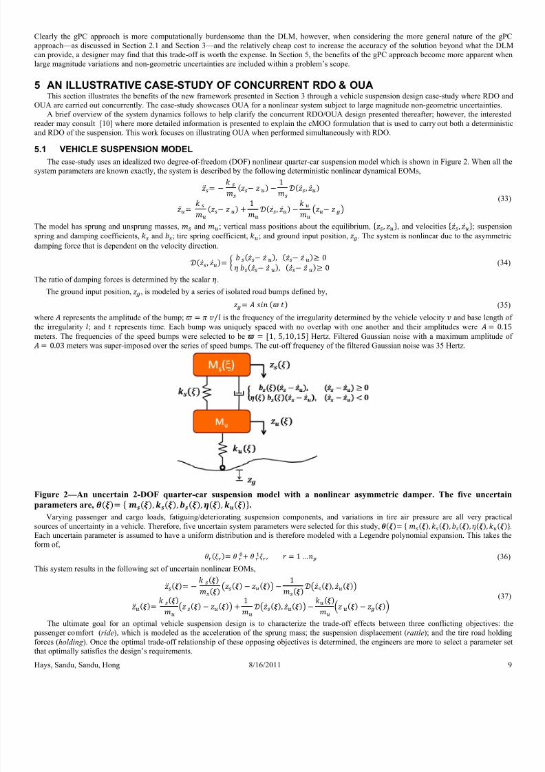
7272019 Simultaneous Optimal Uncertainty Apportionment and Robust Design Optimization (TR 11 15)
httpslidepdfcomreaderfullsimultaneous-optimal-uncertainty-apportionment-and-robust-design-optimization 1115
Hays Sandu Sandu Hong 8162011 10
52 CONCURRENT OUARDO
It is assumed that the standard deviations of the uncertain sprung mass = and tire spring constant = cannot be manipulated by
the design therefore they are treated as fixed uncertainties It is also assumed that the mean nonlinear damping coefficient = is fixed
Therefore the search variables to carry out the OUA are = The same search variables used in [10] for RDO are reused here they
are = The final list of problem search variables is the union of the two sets or cup
There are a number of methods presented in the literature for defining a cost-uncertainty trade-off curve [3] This case-study assumes that thereciprocal power cost-uncertainty trade-off curve used by the manufacturing community is a reasonable definition for the selected non-geometricuncertainties in this case study The reciprocal power curve is defined as
= + = 1 hellip (38)
where is a bias cost associated with the ith source of uncertainty being apportioned is the cost that is scaled by the reciprocal power of the selected
variation magnitude with isin ℝ defining the exponential power Table 3 shows the and values used for the uncertainties associated with =
Table 3mdashIndependent variable means and standard deviations
Parameter Bias ( ) Scaled Cost () Power () 05 140 e+6 15 075 331 e+5 2 085 733 e-1 1
With this selected set of search variables defined cost-uncertainty trade-off curves and uncertain vehicle suspension dynamics described in (37)the corresponding concurrent OUARDO problem may be defined as
983149983145983150
=983163
01011983165
+
s983086 t = minus minus minus 1
= minus + 1 minus minus
=
983156 983142
minus
minus le 0
minus le 0 minus le 0
minus le 0 le le le le 983088 983101 983088 983088 983101 983088
(39
where is a scalarization weighting factor for the ith apportionment cost and the uncertain asymmetric damping force is
= minus minus ge 0 minus minus ge 0 (40)
Therefore (39) simultaneously performs RDO and OUA subject to the uncertain system dynamics defined in (37) and opposing performanceconstraints for vehicle ride rattle and holding In other words (39) determines the optimal apportionment of the uncertainties in
that satisfy
the performance constraints this is accomplished by simultaneously determining optimal nominal suspension values in
Equation (39) is a
robust cMOO formulation in that a Pareto optimal set accounting for the systemrsquos uncertainties may be constructed by sweeping through a range of
the performance constraint bounds Recalling the mean and standard deviation definitions provided in (21)ndash(22) the
performance constraint definitions are μ + σ minus le 0 μ + σ minus μ minus σ minus le 0
minus μ minus σ minus μ + σ le 0 μ + σ minus le 0
(41)
Therefore the performance constraints bound the mean values plus or minus a weighted standard deviation The constants are weighting factors o
the standard deviations setting 983102 10 yields a more conservative design The interested reader is referred to [10] for more details regarding thedefinition of the uncertain performance constraints and this approach to robust cMOO
7272019 Simultaneous Optimal Uncertainty Apportionment and Robust Design Optimization (TR 11 15)
httpslidepdfcomreaderfullsimultaneous-optimal-uncertainty-apportionment-and-robust-design-optimization 1215
Hays Sandu Sandu Hong
53 RESULTS
The following results show the progression of tfinally the concurrent OUARDO design based on thfrom the three designs in the following figures thesimultaneous OUARDA is referenced as aOpt
Figure 3 presents a specific 3D optimal soluti minus minus this solution0203 and = 0034 The dOpt sol
uOpt solution is represented by an asterisk When
dimensions are determined by the original non-optimlines Upon close inspection of Figure 3 it is appare
solution was pushed to a significantly lower
Figure 3mdash Projection of the 3D dOpt uOpt
solutions were determined when = each solution has a different set of active con
Finally the optimal mean solution obtained fromwhen all weighting factors are set to
= 1 the m
apportioned uncertainty standard deviations Tuncertainties for the aOpt solution are significantly land holding constraints Figure 3 confirms that
therefore the simultaneous search finds the true opti
A Pareto optimal trade-off curve may be obtai performance constraints the actual Pareto trade-off
OUARDO optimal solution is determined for a ra
illustrated as a 2D projection into the objectiverattle
Figure 4mdashA single 2D plane from the 5D P
rattle constraint bound the other constraint
two points on the curve are set to zero as thes
983088
983093
983089983088
983089983093
983090983088
983088983086983089983092
983107 983151 983155 983156 983085 983156 983151
983085 983138 983157 983145 983148 983140 983131 983076 983133
8162011
e suspension design from a deterministic optimal performance new framework Figure 3 best helps visualize the difference
deterministic design optimization is referenced as dOpt RD
on in the constraint space as projections onto the three ort
is obtained when the bounding constraints are set to =tion is represented by a solid dot and results in an active hol
all weighting factors are set to
= 1 the mean solution is
al uncertainty standard deviations The projections of the uOpt t that the uOpt solution has an active rattle constraint Since
value when compared to the deterministic value
and aOpt optimal solutions onto the three orthogon = = and traints
the new framework for a simultaneous OUARDO design is r ean solution is enclosed in a 3D cuboid whose dimensions
he projections of the aOpt cuboid are denoted by the dashed lirger than the uOpt solution Also the result of the uncertaintyand are coupled in that the aOpt solution is shifted whenal solution
ed by sweeping through a range of values of the boundingis a 5D surface however to illustrate the ride and holdin
ge of values of the rattle bound where = Th
plane this is illustrated in Figure 4
areto optimal set showing the trade-off between the
s are held constant at = and e resulted in infeasible aOpt designs
983088983086983089983094 983088983086983089983096 983088983086983090 983088983086983090983090 983088983086983090983092
983154983137983156983156983148983141 983131983149983133
983107983151983155983156 983131983076983133
11
design to an RDO design and between the solutions obtainedis referenced as uOpt and the
hogonal 2D planes minus20 = =ing constraint The mean of the
enclosed in a 3D cuboid whose
cuboid are denoted by the dottedthe is so large the uOp
l 2D planes These optima= Notice how
presented by a diamond Againre determined by the optimally
nes Notice how the apportionedapportionment yields active ride
compared to that found by uOpt
onstraints Since there are four g constraints are fixed and the
resulting Pareto curve may be
cost-to-build objective and
= The firs
7272019 Simultaneous Optimal Uncertainty Apportionment and Robust Design Optimization (TR 11 15)
httpslidepdfcomreaderfullsimultaneous-optimal-uncertainty-apportionment-and-robust-design-optimization 1315
Hays Sandu Sandu Hong 8162011 12
One interesting observation is that the OUARDO framework determined the first two design points shown in Figure 4 to be infeasible pointstherefore their values were set to the objective value that results if no optimization was performed The reason for these infeasible constraints is bestillustrated by Figure 5 which shows the 2D projection of the uOpt ride objective trade-off with the rattle constraint resulting from an RDO or uOpt
design [10] the holding bound is fixed at = 0034 The diamond curve is obtained from a dOpt optimal design and the square curve is
obtained from the RDO design however the triangle line shows the bounding constraint value assigned for the OUARDO or aOpt design ( =220 ) When the ride bound (triangle line) is below the uOpt curve (square curve) the OUARDO design requires the uncertainties to be
reduced or tightened to satisfy the constraints However since the variations of the uncertain mass and tire spring constant were assumedto be uncontrollable the required uncertainty reductions for the first two points ended up being infeasible
The resulting optimally allocated uncertainties for the various design points illustrated in Figure 4 are shown in Figure 6 The optimal distributionof the allocated uncertainties is a function of the selected cost-uncertainty trade-off curves defined by (38) and each associated weighting factor
Table 4 documents the apportionment results obtained from the specific case when = 220 = = 0203 and
= 0034 The final apportionment of optimal standard deviations resulted in changes as large as 300 relative to their respective initial
values and as large as 64 relative to their respective mean values this clearly show-cases the new concurrent OUARDO frameworkrsquos ability totreat uncertainties with large magnitudes
Figure 5mdashA single 2D plane showing the trade-off between the ride objective and rattle constraint bound when performing an
RDO design where = is held fixed The triangle curve represents the bounding value for when
performing the OUARDO designs associated with Figure 3 and Figure 4 The first two points on the triangle curve require
too large of a reduction in uncertainties and therefore result in infeasible aOpt designs
The final resulting cost-to-manufacture for the dOpt and uOpt designs was $1770 this is based on the initial non-optimal uncertainty levelswhich apply to both designs However the aOpt solutions result in significant cost-to-manufacture reductions Figure 4 shows the cost savings forthe various design points where savings as high as 74 were experienced Clearly the actual cost-savings achievable by applying the new
simultaneous OUARDO framework defined in (28) (29) or (31) is very dependent upon the definition of the respective cost-uncertainty trade-ofcurves however this case-study illustrates the power of treating uncertainty up-front during the design process robust optimally performing systemsare designed at an optimal cost-to-manufacture
Figure 6mdashOptimally apportioned uncertainties determined from the new simultaneous OUARDO framework The first tw
points were infeasible designs and therefore the values were set to their initial values
Table 4mdashApportionment results obtained from the new concurrent OUARDO framework corresponding to the case when
= = = and = from
non-optimal
from
non-optimal from 11250 30000 6427
983089983093983088
983089983095983088
983089983097983088
983090983089983088
983090983091983088
983090983093983088
983088983086983089983092 983088983086983089983097 983088983086983090983092
983154 983145 983140 983141 983131 983149 983133
983154983137983156983156983148983141 983131983149983133
983140983151983152983156983157983119983152983156983137983119983152983156
983088
983090983088983088983088
983092983088983088983088
983094983088983088983088
983096983088983088983088
983089983088983088983088983088
983089983090983088983088983088
983089983092983088983088983088
983089983094983088983088983088
983088983086983089983092 983088983086983089983094 983088983086983089983096 983088983086983090 983088983086983090983090 983088983086983090983092
983155 983156 983140 983080 983086 983081
983154983137983156983156983148983141 983131983149983133
983155983156983140983080983147983155983081
983155983156983140983080983141983156983137983081
983155983156983140983080983138983155983081
7272019 Simultaneous Optimal Uncertainty Apportionment and Robust Design Optimization (TR 11 15)
httpslidepdfcomreaderfullsimultaneous-optimal-uncertainty-apportionment-and-robust-design-optimization 1415
Hays Sandu Sandu Hong 8162011 13
4230763 2019 2970 05213 30012 5000
6 CONCLUSIONSThis work presents a novel framework that enables RDO concurrently with OUA for dynamical systems described by ODEs Current state of the
art methodologies are limited to only treating geometric uncertainties of small magnitude The new framework removes these limitations by treating both geometric and non-geometric uncertainties in a unified manner within a concurrent RDOOUA setting Additionally uncertainties may berelatively large in magnitude and the system constitutive relations may be highly nonlinear The vehicle suspension design case-study supports thismessage uncertainty allocations on the order of 300 of the initial value were obtained
The computational efficiency of the selected gPC approach allows statistical moments of the uncertain system to be explicitly included in theoptimization-based design process The framework presented in a cMOO formulation enables a Pareto optimal trade-off surface characterization forthe entire family of systems within the probability space The Pareto trade-off surface from the new framework is shown to be off-set from thetraditional deterministic optimal trade-off surface as a result of the additional statistical moment information formulated into the objective andconstraint relations As such the vehicle suspension case-study Pareto trade-off surface from the new framework enables a more robust and optimally
performing design at an optimal manufacturing costIn future work the authors will expand the new framework to treat constrained dynamical systems described by differential algebraic equations
(DAEs)
ACKNOWLEDGEMENTSThis work was partially supported by the Automotive Research Center (ARC) Thrust Area 1 the National Science Foundation (NSF) the
Computational Science Laboratory (CSL) Advanced Vehicle Dynamics Laboratory (AVDL) and the Robotics and Mechanisms laboratory(RoMeLa) at Virginia Tech
REFERENCES[1] Chase K W 1999 Dimensioning and Tolerancing Handbook McGraw-Hill Professional Minimum-Cost Tolerance Allocation[2] Chase K W 1999 Tolerance Allocation Methods for Designers ADCATS Report 99(6) pp 1-28[3] Chase K W Greenwood W H Loosli B G and Hauglund L F 1990 Least Cost Tolerance Allocation for Mechanical Assemblies withAutomated Process Selection Manufacturing Review 3(1) pp 49-59[4] Barraja M and Vallance R R 2002 Tolerance Allocation for Kinematic Couplings eds pp[5] Merkley K G 1998 Tolerance Analysis of Compliant Assemblies PhD thesis Citeseer[6] Krishnaswami P and Kelkar A G 2003 Optimal Design of Controlled Multibody Dynamic Systems for Performance Robustness andTolerancing Engineering with Computers 19(1) pp 26-34[7] Arenbeck H Missoum S Basudhar A and Nikravesh P 2010 Reliability-Based Optimal Design and Tolerancing for Multibody SystemsUsing Explicit Design Space Decomposition Journal of Mechanical Design 132(2) pp 021010-11[8] Lee S J Gilmore B J and Ogot M M 1993 Dimensional Tolerance Allocation of Stochastic Dynamic Mechanical Systems throughPerformance and Sensitivity Analysis Journal of Mechanical Design 115(3) pp 392-402[9] Rout B and Mittal R 2010 Simultaneous Selection of Optimal Parameters and Tolerance of Manipulator Using Evolutionary OptimizationTechnique Structural and Multidisciplinary Optimization 40(1) pp 513-528
[10] Hays J Sandu A Sandu C and Hong D 2011 Parametric Design Optimization of Uncertain Ordinary Differential Equation SystemsTechnical Report No TR-11-06 Virginia Tech Blacksburg VA USA[11] Hays J Sandu A Sandu C and Hong D 2011 Motion Planning of Uncertain Fully-Actuated Dynamical Systemsmdashan Inverse DynamicsFormulation eds Washington DC USA pp (accepted)[12] Hays J Sandu A Sandu C and Hong D 2011 Motion Planning of Uncertain Fully-Actuated Dynamical Systemsmdasha Forward DynamicsFormulation eds Washington DC USA pp (accepted)[13] Hays J Sandu A Sandu C and Hong D 2011 Motion Planning of Uncertain under-Actuated Dynamical Systemsmdasha Hybrid DynamicsFormulation eds Denver CO USA pp (submitted)[14] Hays J Sandu A Sandu C and Hong D 2011 Motion Planning of Uncertain Ordinary Differential Equation Systems Technical Report
No TR-11-04 Virginia Tech Blacksburg VA USA[15] Wiener N 1938 The Homogeneous Chaos American Journal of Mathematics 60(4) pp 897-936[16] Xiu D and Karniadakis G 2003 The Wiener-Askey Polynomial Chaos for Stochastic Differential Equations pp[17] Sandu C Sandu A and Ahmadian M 2006 Modeling Multibody Systems with Uncertainties Part Ii Numerical Applications MultibodySystem Dynamics 15(3) pp 241-262[18] Sandu A Sandu C and Ahmadian M 2006 Modeling Multibody Systems with Uncertainties Part I Theoretical and ComputationalAspects Multibody System Dynamics 15(4) pp 369-391[19] Cheng H and Sandu A 2009 Efficient Uncertainty Quantification with the Polynomial Chaos Method for Stiff Systems Mathematics andComputers in Simulation 79(11) pp 3278-3295[20] Cheng H and Sandu A 2007 Numerical Study of Uncertainty Quantification Techniques for Implicit Stiff Systems eds Winston-Salem
NC USA pp 367-372[21] Cheng H and Sandu A 2009 Uncertainty Quantification in 3d Air Quality Models Using Polynomial Chaoses Environmental Modelingand Software 24(8) pp 917-925[22] Cheng H and Sandu A 2009 Uncertainty Apportionment for Air Quality Forecast Models eds Honolulu HI USA pp 956-960[23] Cheng H and Sandu A 2010 Collocation Least-Squares Polynomial Chaos Method eds Orlando FL USA pp 80[24] Xiu D and Hesthaven J S 2005 High-Order Collocation Methods for Differential Equations with Random Inputs SIAM Journal onScientific Computing 27(3) pp 1118-1139[25] Xiu D 2007 Efficient Collocational Approach for Parametric Uncertainty Analysis Communications in Computational Physics 2(2) pp293-309
7272019 Simultaneous Optimal Uncertainty Apportionment and Robust Design Optimization (TR 11 15)
httpslidepdfcomreaderfullsimultaneous-optimal-uncertainty-apportionment-and-robust-design-optimization 1515
Hays Sandu Sandu Hong 8162011 14
[26] Xiu D 2009 Fast Numerical Methods for Stochastic Computations A Review Communications in Computational Physics 5(2-4) pp 242-272[27] Papoulis A Pillai S and Unnikrishna S 2002 Probability Random Variables and Stochastic Processes McGraw-Hill New York[28] Law M 1996 Multivariate Statistical Analysis of Assembly Tolerance Specifications PhD thesis Brigham Young University Provo UTUSA[29] Greenwood D 2003 Advanced Dynamics Cambridge Univ Pr[30] Murray R Li Z Sastry S and Sastry S 1994 A Mathematical Introduction to Robotic Manipulation CRC Press Inc Boca Raton FLUSA[31] Nikravesh P E 2004 Product Engineering Springer An Overview of Several Formulations for Multibody Dynamics[32] Haug E J 1989 Computer Aided Kinematics and Dynamics of Mechanical Systems Vol 1 Basic Methods Allyn amp Bacon Inc[33] Diehl M Ferreau H and Haverbeke N 2009 Efficient Numerical Methods for Nonlinear Mpc and Moving Horizon Estimation Nonlinear
Model Predictive Control pp 391-417[34] Biegler L T 2003 Optimization of OdeDae Constrained Models Technical Report No[35] Biegler L T and Grossmann I E 2004 Retrospective on Optimization Computers amp Chemical Engineering 28(8) pp 1169-1192[36] Adcats 2006 One-Way Clutch Verification httpadcatsetbyueduWWWADCATSExample_ProblemsProE_Verify2clutch2clutchhtml
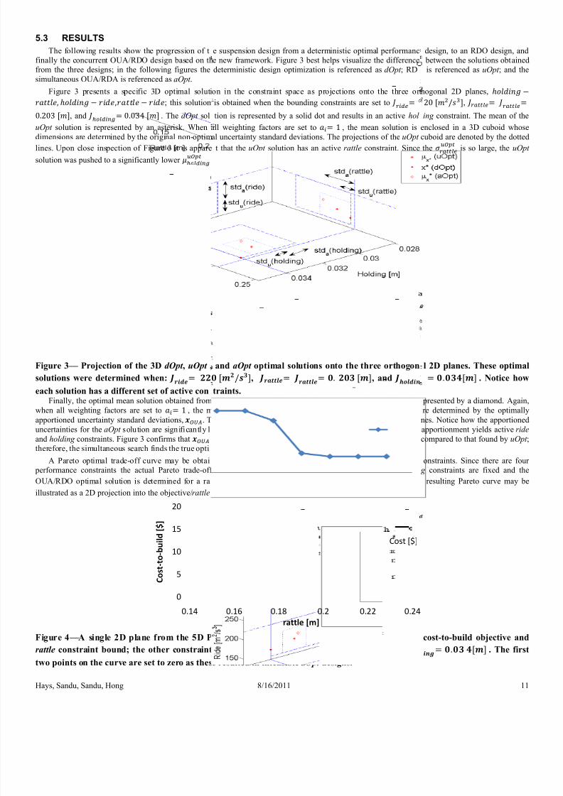
7272019 Simultaneous Optimal Uncertainty Apportionment and Robust Design Optimization (TR 11 15)
httpslidepdfcomreaderfullsimultaneous-optimal-uncertainty-apportionment-and-robust-design-optimization 1515
Hays Sandu Sandu Hong 8162011 14
[26] Xiu D 2009 Fast Numerical Methods for Stochastic Computations A Review Communications in Computational Physics 5(2-4) pp 242-272[27] Papoulis A Pillai S and Unnikrishna S 2002 Probability Random Variables and Stochastic Processes McGraw-Hill New York[28] Law M 1996 Multivariate Statistical Analysis of Assembly Tolerance Specifications PhD thesis Brigham Young University Provo UTUSA[29] Greenwood D 2003 Advanced Dynamics Cambridge Univ Pr[30] Murray R Li Z Sastry S and Sastry S 1994 A Mathematical Introduction to Robotic Manipulation CRC Press Inc Boca Raton FLUSA[31] Nikravesh P E 2004 Product Engineering Springer An Overview of Several Formulations for Multibody Dynamics[32] Haug E J 1989 Computer Aided Kinematics and Dynamics of Mechanical Systems Vol 1 Basic Methods Allyn amp Bacon Inc[33] Diehl M Ferreau H and Haverbeke N 2009 Efficient Numerical Methods for Nonlinear Mpc and Moving Horizon Estimation Nonlinear
Model Predictive Control pp 391-417[34] Biegler L T 2003 Optimization of OdeDae Constrained Models Technical Report No[35] Biegler L T and Grossmann I E 2004 Retrospective on Optimization Computers amp Chemical Engineering 28(8) pp 1169-1192[36] Adcats 2006 One-Way Clutch Verification httpadcatsetbyueduWWWADCATSExample_ProblemsProE_Verify2clutch2clutchhtml