SIMULTANEOUS MOMENTUM AND ENERGY TRANSFER … · simultaneous momentum and energy transfer analysis...

ENCICLOPÉDIA BIOSFERA , Centro Científico Conhecer - Goiânia, v.13 n.23; p. 2016

1668

SIMULTANEOUS MOMENTUM AND ENERGY TRANSFER ANALYSIS IN A DISTILLATION COLUMN SIEVE TRAY USING CFD TECHNIQUES : STUDY OF

INFLUENCE OF THE INLET DOWNCOMER

Gabriel Henrique Justi1, Conrado Planas Zanutto2, Gabriela Cantarelli Lopes3, José Antônio Silveira Gonçalves4

1 Ph.D. candidate in chemical engineering at the Federal University of São Carlos ([email protected]) São Carlos - Brazil

2 Ph.D. candidate in mechanical engineering at the Federal University of Santa Catarina - Brazil

3 Professor, chemical engineering at the Federal University of São Carlos ([email protected]) São Carlos - Brazil

4 Professor, chemical engineering at the Federal University of São Carlos ([email protected]) São Carlos - Brazil

Recebido em: 08/04/2016 – Aprovado em: 30/05/2016 – Publicado em: 20/06/2016 DOI: 10.18677/Enciclopedia_Biosfera_2016_150

ABSTRACT Efficient and economical performance of distillation equipment is vital to many processes. Distillation is one of the unit operations most used separation techniques of components. Its great importance is due to the capacity of purify components of a mixture using the volatility difference among them as driving force. Due to the development of the information technology (IT), in the numerical methods and improvement in models of multiphase flows, the investigation of complex turbulent flow problems is possible. One way to investigate these problems is to use the computational fluid dynamics (CFD) tecniques. That way, it was adopted for this study a CFD model, with the main objective to evaluate the transport phenomena for the non-isothermal flows (ethanol-water) through the CFD techniques to simulate a distillation sieve tray. The proposed model is based in a heterogeneous, three-dimensional, SST turbulence model, and Eulerian-Eulerian framework at 1 atm. The continuity and momentum and energy conservation equations were used to describe the flow. The simulated geometry was based on experimental work of Solari e Bell (1986), to which they were observed the influence with and without of the inlet downcomer on sieve tray. The results showed besides the hydraulic parameters, the temperature profiles. Thus, the simulations of the indicated a strong influence of the liquid velocity profile on the temperature fields on sieve tray for the domain with the downcomer inlet. The methodology used in this work showed adequate, being a viable and important tool in the design and optimization of distillation tray. KEYWORDS: CFD, distillation, sieve tray

RESUMO O desempenho eficiente e econômico de uma coluna de destilação é indispensável para muitos processos químicos industriais. A destilação é uma das operações unitárias mais utilizadas na separação de componentes. Sua importância dá-se na capacidade de separar os componentes de uma mistura líquida utilizando a diferença de volatilidade entre eles como força motriz. Com o avanço da tecnologia


1669

de informação (TI), dos métodos numéricos e aperfeiçoamento em modelos de fluxos multifásicos, é possível a investigação de problemas complexos de escoamentos turbulentos. Uma das formas de investigar esses problemas é a aplicação da fluidodinâmica computacional (CFD). Dessa maneira, foi adotado para o presente trabalho um modelo de CFD, tendo como objetivo principal a avaliar os fenômenos de transportes para o escoamento não-isotérmico (etanol-água) através das técnicas de CFD na simulação de um prato perfurado de destilação. O modelo proposto é baseado em um modelo heterogêneo, tridimensional, modelo de turbulência SST e abordagem Euleriana-Euleriana a 1 atm. As equações da continuidade e de conservação da quantidade de movimento e de energia foram empregadas para representar o escoamento. O domínio computacional foi baseados no trabalho de Solari e Bell (1986), ao qual foram observados a influência com e sem o downcomer de entrada no prato perfurado. Os resultados mostraram além dos parâmetros hidráulicos, os perfis de temperatura. Assim, as simulações indicaram uma forte influência do perfil de velocidade de líquido nos campos de temperatura no prato para o domínio com downcomer. A metodologia empregada neste trabalho foi adequada, mostrando-se uma ferramenta viável e importante no desenvolvimento e otimização de pratos de destilação. PALAVRAS-CHAVE: CFD, destilação, prato perfurado

INTRODUCTION Distillation is one of the most important and utilized liquid-liquid separation

techniques. It is a physical process based on the difference of volatility of the components in a mixture and involves momentum, energy, and mass transfer. The preliminary study of tray hydrodynamic is important to avoid critical regions such as recirculation or stagnant regions, which directly affect the separation efficiency of the stage (KISTER, 1992; WANKAT, 2011).

Continuous improvements in computer technology and numerical methods have allowed to deal with physical and chemical phenomena from its fundamental equations on a microscopic scale, through the Computational Fluid Dynamics (CFD) techniques. In this way, many CFD studies on sieve trays have been done in the last years (TU et al., 2012). Thus, in a distillation column sieve tray, liquid falls through the downcomer by gravity from one tray to the other below it. Downcomers play an important role in separation and hydrodynamic behavior of trays, as mass transfer occurs in the downcomer as well as on the tray deck. Thus, it is significant to focus on the simulation systems considering tray hydrodynamics in the presence of downcomers. Inlet downcomer conditions affect the froth height on the bulk of the tray as well as downstream conditions near the exit weir. As liquid flows through the downcomer clearance to the tray deck, a transition from a single phase to two-phase flow occurs which makes the analysis in the region of the liquid entry quite difficult (LOCKETT, 1986).

Some of studies have focused on the understanding of hydrodynamics phenomena that occurs in a distillation sieve trays, making possible the analysis of important factors, such as: velocity distributions, liquid and gas volume fractions profiles along the tray, regions of intense turbulence and regions of liquid accumulation, etc. Those kind of results allow the implementation of improvements in the design of the trays, in order to avoid critical regions that directly affect the mass and energy transfer occurring throughout the stages, such as retrograde flow and stagnant regions (MEHTA et al., 1998; LIU et al., 2000; VAN BATEN & KRISHNA, 2000; GESIT et al., 2003; RAHIMI et al., 2006). In these studies, the authors did not


1670

model the inlet downcomer in the simulations, considering a flat or parabolic liquid inlet velocity profile.

In order to verify the heat transfer of energy along the sieve trays, NORILER et al. (2008) presented a three-dimensional, transient and two-phase flow, in an Eulerian-Eulerian approach. Thus, the continuity equations and the energy and momentum conservation balances were applied for both chemical species, for predictions of volume fractions and velocities, temperatures and pressure fields.

NORILER et al. (2010) analyzed the mass and energy transfers along the sieve tray simultaneously. The authors proposed a transient, 3-D, multiphase, and multicomponent flow, in an Eulerian-Eulerian approach. Thus, the continuity equations and the momentum, energy and chemical species conservation balances were applied for both fluids, for predictions of efficiency and temperature and concentration profiles.

RAHIMI et al. (2011) considered the complete geometry including sieve tray, inlet and outlet downcomers. These were modeled using CFD and based on experimental work of SOLARI & BELL (1986) for air-water system. The authors predicted only the tray hydrodynamics parameters, such as liquid velocity distribution, clear liquid height, average liquid volume fraction in froth and froth height.

The main purpose of this work is to evaluate of the effect of inlet downcomer in the momentum and energy conservation equations on a sieve tray using a two-phase, 3-D (three dimension) and transient CFD model in an Eulerian-Eulerian approach. A water-ethanol liquid mixture at 1 atm was simulated.

MATHEMATICAL MODELING The mathematical model was based on an Eulerian-Eulerian framework the

liquid and gas phases. Thus, each phase was treated as an interpenetrating continuum phase having separate transport equations. Thereat, the Reynolds averaged Navier-Stokes equations (RANS) were included and numerically solved for each phase. Since the pressure gradient is small over a distillation stage, the system was considered at 1 atm. The conservation equations for the phases are given below and the subscript “k” and “j” represents the liquid and gas phase.

Mass continuity equation

( ) ( ) ∑≠

Γ+=ρ⋅∇+ρ∂∂ pn

jkkjk,MSkkkkk ff

tSv (1)

for k = 1,...,np where t, fk, ρk, and vk represent the time (s), volume fraction (-), density (kg.m-3), and velocity vector (m.s-1) for the k phase, respectively. The term SMS,k represents the mass source (kg.m-2.s-2) and Γkj represents the changing mass rate between the phases k and j (kg.m-2.s-2) and “np” is the number of phases. Momentum equation


1671

( ) ( ) ( ) ( )∑∑≠

++

≠

Γ−Γ+ρ++⋅∇+∇−=ρ⋅∇+ρ∂∂ pp n

jkkjkjkjkk

n

jkkj

effkkkkkkkkkkk ffpfff

tvvgMTvvv (2)

for k = 1,...,np

where pk and eff

kT represent the pressure field (kg.m-1.s-2) and the effective flux of momentum (kg.m-2.s-1), respectively. Mkj is the momentum transfer between phases (kg.m-2.s-2), the term ( kjkjkj vv ++ Γ−Γ ) is the momentum transfer rate between the

phases due to the mass transfer between phases (kg.m-2.s-2), and g is the gravity vector (m.s-2). Energy equation

( ) ( ) ( ) ( )∑∑≠

++

≠Γ−Γ+++⋅∇=ρ⋅∇+ρ

∂∂ pp n

jkk,sjkj,skjk,E

n

jkkj

effkkkkkkkkk hhfhfhf

tSQqv (3)

for k = 1,...,np

where hk is the enthalpy of the phase k (J.kg-1), eff

kq represents effective flux of energy (J.m-2.s-1), Qkj is the energy transfer between phases (J.m-3.s-1), and the term ( k,sjkj,skj hh ++ Γ−Γ ) represents the energy transfer between the phases due the mass

transfer between the phases (J.m-3.s-1). Constraint equations

The gas and liquid volume fractions are related through the summation constraint:

1fpn

1kk =∑

=

(4)

For the pressure constraint, the same pressure field has been assumed for

both phases, i.e.,

ppp jk == (5)

Model assumptions

The following assumptions were adopted on the model used in this study for a sieve tray:

a) a two-phase system was modeled in the simulation;

b) the gas phase is the dispersed phase and the liquid phase is the continuous phase;

c) a ethanol/water liquid mixture was used in this study;

d) due to the fact that there are no reactions and no other mass source, the terms SMS (Equation 1) and SE (Equation 3) are nulls;

e) the net rate of the mass transfer between the phases is considered to be small and in this study the modeling of chemical species tranfer were not


1672

included. In this case, the right-hand side of Equation 1 vanishes and the terms associated with it in Equations 2 and 3 are nulls;

f) no turbulence model was used for dispersed phase.

Closure equations In order to solve some terms of the Equations 2 and 3 additional equations are

required. In this way, the terms that need to be modeled, such as effective fluxes of momentum (Teff) and energy (qeff), interphase momentum transfer (Mk), and interphase energy transfer (Qk) are presented below.

Effective flux of momentum

The effective fluxes are related to the dispersion of the properties due to viscous and turbulent effects. Thus, it can be written as a combination between diffusion flux and turbulent flux, where the “turb” superscript represents turbulent flux. Considering a Newtonian fluid and the eddy viscosity hypothesis, the effective flux of momentum can be written as:

( )( )tpkk

effk

turbkk

effk vvTTT ∇+∇µ=+= (6)

where eff

kµ represent the effective viscosity (kg.m-1.s-1) in the k phase and tp is the transpose of vector.

The effective viscosity term can be expressed by:

turbkk

effk µ+µ=µ (7)

where kµ and turb

kµ represents the molecular viscosity (kg.m-1.s-1) and the turbulent viscosity (kg.m-1.s-1), respectively.

The turbulent viscosity, turbkµ , is then modeled using a turbulence model. The

Shear Stress Transport (SST) turbulence model was used to describe the turbulence on the sieve tray. This turbulence model combines the advantages of the ε−k and

ω−k models, with a possibility to describe accurately regions that are near the wall:

( )2k1

kk1turbk SF;max

kωαρα=µ (8)

where 1α , kk , kω , S, and F2 represent the model constant (dimensionless), the turbulence kinetic energy (m2.s-2), the turbulent frequency (s-1) for the k phase, the invariant measure of the strain rate (dimensionless), and the blending function (dimensionless), respectively. The SST model is well discussed in the literature (MENTER, 1994; WILCOX, 2006).

Effective flux of energy

Similar to the definition of the effective flux of momentum, the effective flux of energy (qeff) can be described below:

keffk

turbkk

effk T∇λ=+= qqq (9)


1673

where eff

kλ and kT represent the effective thermal conductivity (W.m-1.K-1) and temperature (K) in the k phase, respectively.

The effective thermal conductivity can be expressed by,

turbkk

effk λ+λ=λ (10)

where kλ is the thermal conductivity (W.m-1.K-1) and turb

kλ represents the turbulent thermal conductivity (W.m-1.K-1).

From the prediction of the turbulent viscosity (Equation 8) and the concept of the turbulent Prandtl number, it is possible to calculate the turbulent thermal conductivity, as shown in Equation 11:

turb

turbkturb

k Prµ=λ (11)

where turbPr represents the turbulent Prandtl number (dimensionless). Interphase momentum transfer

The interphase momentum transfer term ( kjM ) was considered in this work

only due to the drag force. The drag force per unit volume for gas-liquid flow can be written as:

( ) lglglgB

Dlggl

n

jkkj f

dC

43p

vvvvMMM −−ρ=−==∑≠

(12)

where the subscripts “l” and “g” represent the liquid and gas phases, respectively. CD is the drag coefficient (dimensionless) and dB is the mean bubble diameter (m).

The drag coefficient has been estimated using the Krishna et al. correlation (KRISHNA et al., 1999) as showed below:

2slip

Bl

glD

V

1gd

34

Cρ

ρ−ρ= (13)

where Vslip represents the slip velocity (m.s-1) and it can be estimated from the gas superficial velocity and the average gas holdup fraction in the froth region as,

aveg

sslip f

UV = (14)

where Us is the gas superficial velocity (m.s-1) and ave

vf representes the average gas holdup fraction (dimensionless) in the froth region.


1674

For average gas holdup fraction, the Bennett et al. correlation (BENNETT et al., 1983) was used as follows:

ρ−ρρ

−=91.0

gl

gs

aveg U55.12exp1f (15)

Note that when the drag correlation (Equation 12) is substituted in Equation

11, the mean bubble diameter is canceled, eliminating the main problem in the prediction of gas-liquid bubbling flow. Interphase energy transfer

Heat transfer between the phases must satisfy the local energy balance. Thus, the rate of energy transfer between phases can be written:

( )lgglgllggl

n

jkkj TTAh

p

−=−==∑≠

QQQ (16)

where hgl and Agl represent global heat transfer coefficient (J.m-2.s-1.K-1), and interfacial area per unit volume (m2.m-3), respectively.

The global heat transfer coefficient is defined as,

B

gllgl d

Nuh

λ= (17)

where Nugl represents Nusselt number (dimensionless).

An appropriate value of the global heat transfer coefficient can be obtained by using suitable correlations, such as Ranz-Marshall equation (RANZ & MARSHALL, 1952):

( ) ( ) 3.0g

5.0ggl PrRe6.02Nu += (18)

250Pr0and200Re0

for

gg ≤≤≤≤

where Reg and Prg are Reynolds (dimensionless) and Prandtl (dimensionless) numbers, respectively.

The dimensionless numbers are defined as,

l

Blgl

g

dvvRe

µ

−ρ= (19)

g

gg,pg

CPr

λµ

= (20)

where Cp,g representes gas heat capacity (J.kg-1.K-1).


1675

The interfacial area per unit volume between liquid and gas phases, known as the interfacial area density (Agl) for the particle model, it is defined by:

B

ggl d

f6A = (21)

The mean bubble diameter, dB, can be estimated relating it to the maximum bubble diameter, dB,max, which is modeled by the correlation (Equation 22) proposed by DAVIDSON & SCHÜLER (1960),

2

dd max,B

B = (22)

5

2

B

Cs

4t

max,B AA

Ug

p23.1d

= (23)

where pt, AC, and, AB represent the triangular pitch (m), the column cross-section area (m2), and the bubbling area (m2), respectively.

NUMERICAL METHODOLOGY Computational domain and numerical mesh

The computational domains consist of a distillation sieve tray with diameter of 0.40 m. The 3-D geometry was developed using the software ANSYS Design Modeler. Table 1 presents the specifications of the sieve tray geometry and Figure 1 shows the geometries used in the simulations.

(a) (b)

FIGURE 1 - Computational domain, mesh and boundary conditions: (a) without inlet downcomer and (b) with inlet downcomer

Both the geometry with and without the inlet downcomer were simulated. The tray has a 75% of bubbling area, a weir height of 0.015 m, a downcomer clearance of 0.01 m, a 4.06% hole area with 0.005 m (length) rectangular holes arranged in a 0.025 m triangular pitch.


1676

TABLE 1 - Distillation sieve tray specifications Description Units

Tray diameter 0.40 m Tray spacing 0.19 m Weir height 0.3091 m Weir lenght 0.015 m Downcomer clearance 0.01 m Downcomer lenght 0.18 m Flow path lenght 0.2539 m Hole lenght and triangular pitch 0.005×0.025∆ m % Bubbling area (over total area) 75 % % Hole area (over bubbling area) 4.06 %

The grid used in the simulation was developed using the software ANSYS Meshing and consists in a hybrid grid with triangular prism and hexahedral elements. Figure 1 shows the details of the numerical mesh. Further on, sensitivity test to different grid sizes will be presented.

Boundary and initial conditions Figure 1 illustrates the boundary regions of the sieve tray. Liquid enters the

tray through the downcomer clearance area (labeled as Liquid Inlet), and leaves the tray through the downcomer clearance area that leads to the tray below (labeled as Liquid Outlet). Gas enters through holes at the bottom of the tray (labeled as Gas Inlet), and leaves the domain through holes at the top (labeled as Gas Outlet).

Gas inlet The gas mass flow rate entering through the holes on the tray is the same in

each hole. Thus, the gas velocity that flows through the holes was calculated according to Equation 24. It was considered that only the gas phase enters this region, once the amount of liquid dragged by the gas is negligible. Additionally, it was specified that the mass fraction of ethanol in the gas phase was 0.7330.

i,HH

Bsinlet,g AN

AUV = (24)

where Vg,inlet, NH, and AH,i represent gas inlet velocity (m.s-1), total number of holes (dimensionless), and a hole area (m2), respectively.

Gas Outlets A pressure condition was used for gas outlet, specifying a relative pressure of

zero.

Liquid inlet At the liquid inlet in the Figure 1, only liquid was adopted a uniform velocity

profile according to Equation 25. It was considered that only liquid phase enters this region, once the amount of dragged liquid by the gas is negligible. Additionally, it was specified that the mass fraction of ethanol in the liquid phase was 0.5402.

cl

linlet,l A

QU = (25)


1677

where Ul,inlet, Ql, and Acl represent liquid inlet velocity (m.s-1), liquid volumetric flow rate (m3.s-1), and liquid inlet area (m2), respectively. Liquid Outlet

At the liquid outlet region, a pressure condition was adopted in order to simulate a resistance, which actually exists due to the lower tray. The resistance involves the emergence of a buildup of fluid column in the downcomer outlet.In this work was considered occupying of 50% of the outlet downcomer length.

Walls A no-slip wall was specified for both phases.

Domain initialization Good initial estimates of the flow variables are important not only to avoid a

significantly longer computational time but also in some cases to avoid divergence. The initial condition applied in the simulation consisted of the domain filled only with stopped gas phase at a temperature of the 356.80 K. Thus, it was possible to observe the tray filling by the liquid phase. Simulation settings

The simulation settings were established using the ANSYS software CFX-Pre 14.5. The following strategy to minimize computational effort and to ensure the solution stability has been adopted. First of all, it was obtained the solution for the flow without considering the energy equation, until reaching the quasi-steady condition. This result was used as initial condition for the next step which consisted in the solution of the model equations with the energy equation. The operation conditions used in the simulation were a liquid volumetric flow rate, Ql, equal to 7.5×10-4 m3.s-1, and a gas load factor F-factor, FS, equal to 0.8 m.s-1(kg.m-3)0.5. The FS is defined (Equation 26) as a function of the gas superficial velocity and the gas density, i.e.,

gss UF ρ= (26)

Physical properties of liquid and gas phases used in the simulation are presented in Table 2. The superscripts “inlet”, “A” and, “mix” represent the inlet region in the computational domain, the chemical species ethanol, and the mixture properties, respectively.

TABLE 2 - Physical properties of liquid and gas phases Physical properties Liquid Gas Units

Temperature Tinlet 354.80 356.90 K XA,inlet 0.5402 - - Ethanol mass fraction YA,inlet - 0.7330 -

Heat capacity Cp,mix 3558.53 1692.59 J.kg-1.K-1 Density ρmix 839.28 1.292 kg.m-3 Dynamic viscosity µmix 3.790×10-4 1.070×10-4 kg.m-1.s-1 Thermal conductivity λmix 0.3955 0.0207 W.m-1.K-1 Diffusivity DAB 6.709×10-9 1.576×10-5 m2.s-1

For the continuity, momentum and energy the equations, the upwind interpolation scheme was used for the advective terms and First Order Backward


1678

Euler scheme was employed for the transient terms. For the equations related to turbulence, the High Resolution scheme was used. The coupled solution method was used to solve the model, with all the equations solved simultaneously as a single system. The simulation was conducted using thirty-two AMD Opteron 2.40 GHz processors running (32×2.40 GHz) in parallel to simulate 10 seconds of multiphase flow on a distillation sieve tray using fixed time steps of 0.002 s. The Courant number used in the simulations was 0.5.

RESULTS AND DISCUSSION A grid-size sensitivity test was performed using the GCI (Grid Convergence

Index) method proposed by Roache (ROACHE, 1994) to quantify the numerical uncertainty. After the choice of the mesh, simulations of the sieve trays with and without the inlet downcomer were carried out to observe the effects of including this region at the computational domain in order to better understand the flow patterns and temperature profiles throughout the stage.

Grid-size sensitivity test To evaluate the stability of the numerical grid, the clear liquid height (in an

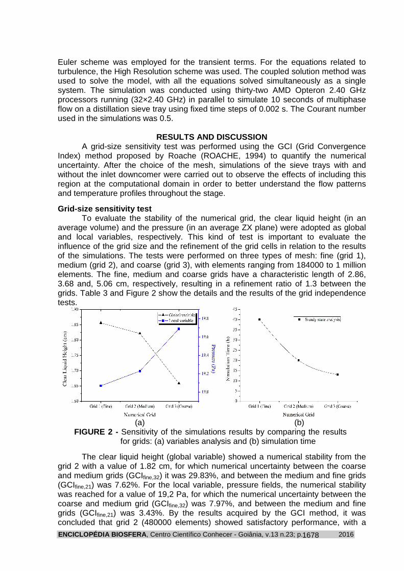
average volume) and the pressure (in an average ZX plane) were adopted as global and local variables, respectively. This kind of test is important to evaluate the influence of the grid size and the refinement of the grid cells in relation to the results of the simulations. The tests were performed on three types of mesh: fine (grid 1), medium (grid 2), and coarse (grid 3), with elements ranging from 184000 to 1 million elements. The fine, medium and coarse grids have a characteristic length of 2.86, 3.68 and, 5.06 cm, respectively, resulting in a refinement ratio of 1.3 between the grids. Table 3 and Figure 2 show the details and the results of the grid independence tests.

(a) (b)

FIGURE 2 - Sensitivity of the simulations results by comparing the results for grids: (a) variables analysis and (b) simulation time

The clear liquid height (global variable) showed a numerical stability from the grid 2 with a value of 1.82 cm, for which numerical uncertainty between the coarse and medium grids (GCIfine,32) it was 29.83%, and between the medium and fine grids (GCIfine,21) was 7.62%. For the local variable, pressure fields, the numerical stability was reached for a value of 19,2 Pa, for which the numerical uncertainty between the coarse and medium grid (GCIfine,32) was 7.97%, and between the medium and fine grids (GCIfine,21) was 3.43%. By the results acquired by the GCI method, it was concluded that grid 2 (480000 elements) showed satisfactory performance, with a


1679

numerical uncertainty below 8% compared with the grid 1 (fine) for global and local variables, as shown in Table 3.

TABLE 3 - Numerical uncertainty calculation applied to the grid under analysis

Variables Location GCI fine,32 GCIfine,21 Clear liquid height - 29.83% 7.62% Pressure YZ plane (x = 0 m) 7.97% 3.43%

In addition, as the computation time is of great importance in optimizing the simulation, it is noteworthy that grid 2 had a processing time (see Figure 2b) approximately two times lower than that grid 1 to obtain similar results.

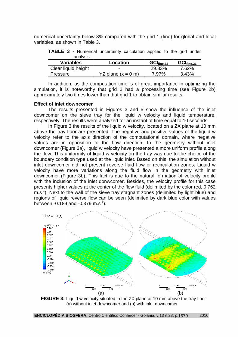
Effect of inlet downcomer The results presented in Figures 3 and 5 show the influence of the inlet

downcomer on the sieve tray for the liquid w velocity and liquid temperature, respectively. The results were analyzed for an instant of time equal to 10 seconds.

In Figure 3 the results of the liquid w velocity, located on a ZX plane at 10 mm above the tray floor are presented. The negative and positive values of the liquid w velocity refer to the axis direction of the computational domain, where negative values are in opposition to the flow direction. In the geometry without inlet downcomer (Figure 3a), liquid w velocity have presented a more uniform profile along the flow. This uniformity of liquid w velocity on the tray was due to the choice of the boundary condition type used at the liquid inlet. Based on this, the simulation without inlet downcomer did not present reverse fluid flow or recirculation zones. Liquid w velocity have more variations along the fluid flow in the geometry with inlet downcomer (Figure 3b). This fact is due to the natural formation of velocity profile with the inclusion of the inlet donwcomer. Besides, the velocity profile for this case presents higher values at the center of the flow fluid (delimited by the color red, 0.762 m.s-1). Next to the wall of the sieve tray stagnant zones (delimited by light blue) and regions of liquid reverse flow can be seen (delimited by dark blue color with values between -0.189 and -0.379 m.s-1).

(a) (b)

FIGURE 3: Liquid w velocity situated in the ZX plane at 10 mm above the tray floor: (a) without inlet downcomer and (b) with inlet downcomer


1680

The liquid w velocity profiles for the sieve tray with and without inlet downcomer can be shown in more detail in Figure 4.In Figure 4a the average linear liquid w velocity were measured along lines in parallel (from z = -0.085 to z= 0.085 m) to the liquid flow direction and on a ZX plane (y = 0.01 m) above the tray floor, consisting of nine lines in different positions along the x axis (x = -0.15, -0.1125, -0.075, -0.0375, 0, 0.0375, 0.075, 0.1125, and -0.15 m). In Figure 4b, the abscissa values represent the dimensionless coordinate (x/R), where -1 and 1 represent wall region and 0 represents the center. In Figure 4b the results showed different liquid w velocity profiles for the two geometries. Therefore, if we analyze the liquid w velocity, the tray with inlet downcomer (red line) showed velocity gradients with high values at the central region of the sieve tray (see also Figure 3b) and near the wall of the sieve tray the liquid velocity had a deceleration reaching values close to zero and negative, i.e., regions of stagnant and retrograde liquid flow.

(a) (b) FIGURE 4: Liquid w velocity profile: (a) lines positions of the CFD model and (b)

average linear liquid w velocity along the x axis for the geometries with inlet downcomer (red line) and without Inlet downcomer (black line)

Also in Figure 4b, the geometry without inlet downcomer presented a liquid w velocity profile more uniform (black line) in relation to the x direction.

The liquid temperature profile on the ZX plane (y = 0.01 m) is shown in Figure 5, where temperatures ranged from 354.8 to 355.1 K.

The influence and effects of the inlet downcomer are also observed for the liquid temperature.


1681

(a) (b) FIGURE 5: Liquid temperature profiles situated in the ZX plane at 10 mm above the

tray floor: (a) without inlet downcomer and (b) with inlet downcomer

By analyzing the average liquid temperature at the ZX plane, one can note very close values for the two computational domains, i.e., 354.87 K for the geometry without inlet downcomer and 354.95 K for the geometry with inlet downcomer. However, the temperature patterns are significantly different for the different geometries (Figures 5a and 5b). It highlights how the effects of flow reverse acting on the tray with inlet downcomer alter the liquid temperature profiles along the plate. This influence was due to the increased liquid residence time in the regions near the wall of the tray, allowing greater heat transfer between phases in the sieve tray with the inlet downcomer.

Based on the results obtained and the observations made for the liquid velocity and temperature profiles, the influence and importance of including the inlet downcomer in the computational model becomes evident and it allows a better understanding of the hydrodynamic and thermal behavior in a distillation column sieve tray.

CONCLUSIONS The results presented qualitatively and quantitatively the influence of the

inclusion of the inlet downcomer in the CFD simulation of a distillation column sieve tray. The influence of the inlet downcomer on the mass transfer should be considered in further simulations. It can lead to better results and more realistic conditions compared to that obtained using uniform inlet velocity profile.

Finally, CFD can be applied for a better understanding of the turbulent multiphase flow on the sieve trays and also they can be used to optimize the design and operating conditions.

ACKNOWLEDGMENTS The authors thank the Graduate Program at Federal University of São Carlos

(PPG-EQ/UFSCar), FAPESP, and CAPES.

REFERENCES


1682

BENNETT, D.; AGRAWAL, R.; COOK, P. New pressure drop correlation for sieve tray distillation columns. AIChE Journal , v. 29, n. 3, p. 434-442, 1983. DAVIDSON, J.; MECH, A.; SCHÜLER, B. Bubble formation at an orifice in a viscous liquid. Chemical Engineering Research & Design , v. 38, p. 144-154, 1960. GESIT, G.; NANDAKUMAR, K.; CHUANG, K. T. Cfd modeling of flow patterns and hydraulics of commercial-scale sieve trays. AIChE Journal , v. 49, n. 4, p. 910-924, 2003. KISTER, H. Z. Distillation design. McGraw-Hill Education, 1992. KRISHNA, R.; URSEANU, M.I.; VAN BATEN, J.M.; ELLENBERGUER, J. Rise velocity of a swarm of large gas bubbles in liquids. Chemical Engineering Science , v. 54, n. 2, p. 171-183, 1999. LIU, C. J.; YUAN, X. G.; YU, K. T.; ZHU X. J. A fluid–dynamic model for flow pattern on a distillation tray. Chemical Engineering Science , v. 55, n. 12, p. 2287-2294, 2000. LOCKETT, M. J. Distillation tray fundamentals. Cambridge University Press, 1986. MEHTA, B.; CHUANG, K.; NANDAKUMAR, K. Model for liquid phase flow on sieve trays. Chemical Engineering Research and Design , v. 76, n. 7, p. 843-848, 1998. MENTER, F. R. Two-equation eddy-viscosity turbulence models for engineering applications. The American Institute of Aeronautics and Astronaut ics journal , v. 32, n. 8, p. 1598–1605, 1994. NORILER, D.; BARROS, A. A. C.; WOLF MACIEL, M. R.; MEIER, H. F. Simultaneous momentum, mass, and energy transfer analysis of a distillation sieve tray using cfd techniques: prediction of efficiencies. Industrial and Engineering Chemistry Research , v. 49, n. 14, p. 6599-6611, 2010. NORILER, D.; MEIER, H. F.; BARROS, A. A. C.; WOLF MACIEL MACIEL, M. R. Thermal fluid dynamics analysis of gas–liquid flow on a distillation sieve tray. Chemical Engineering Journal , v. 136, n. 2, p. 133-143, 2008. RAHIMI, R.; AMERI, A.; SETOODEH, N. Effect of inlet downcomer on the hydrodynamic parameters of sieve trays using cfd analysis. Journal of Chemical and Petroleum Engineering , v. 45, n. 1, p. 27-38, 2011. RAHIMI, R.; RAHIMI, M. R.; ZIVDAR, M. Efficiencies of sieve tray distillation columns by CFD simulation. Chemical Engineering and Technology , v. 29, n. 3, p. 326-335, 2006. RANZ, W.; MARSHALL, W. Evaporation from drops. Chemical Engineering Progress , v. 48, n. 3, p. 141-146, 1952.


1683

ROACHE, P. J. Perspective: a method for uniform reporting of grid refinement studies. Journal of Fluids Engineering , v. 116, n. 3, p. 405-413, 1994. SOLARI, R.; BELL, R. Fluid flow patterns and velocity distribution on commercial-scale sieve trays. AIChE Jornal , v. 32, n. 4, p. 640-649, 1986. TU, J.; YEOH, G. H.; LIU, C. Computational fluid dynamics: a practical approach, second ed. Butterworth-Heinemann, 2012. VAN BATEN, J. V.; KRISHNA, R. Modelling sieve tray hydraulics using computational fluid dynamics. Chemical Engineering Journal , v. 77, n. 3, p. 143-151, 2000. WANKAT, P. C. Separation process engineering: includes mass transfer analysis, third ed. Prentice Hall, 2011. WILCOX, D. C. Turbulence modeling for CFD, third ed. DCW Industries, 2006.

SIMULTANEOUS MOMENTUM AND ENERGY TRANSFER … · simultaneous momentum and energy transfer analysis...

Documents

Transcript of SIMULTANEOUS MOMENTUM AND ENERGY TRANSFER … · simultaneous momentum and energy transfer analysis...