TraceAd Tag Coordinator Collaborate With Any Media Or Technology You Choose
Upload
beverly-lawsonCategory
view
228download
0
Simultaneous games with continuous strategies
• Suppose two players have to choose a number between 0 and 100. They can choose any real number (i.e. any decimal). • They have continuous strategies
• If they choose the same number than player 1 wins $1000. Otherwise player 1 gets nothing.
• If the numbers sum to 100 then player 2 wins $1000. Otherwise player 2 gets nothing.
How do we model this game?

Best response function for player 1
• If player 2 plays 33, then player 1’s ‘best response’ is to play 33
• If player 2 plays 74.5 then player 1’s ‘best response’ is to play 74.5 … and so on.
• Player 1’s best response function tells us, for every possible action by player 2, what is the best response of player 1

Best response function for player 1
Player 1
Player 20
100
100
The ‘45 degree line’ gives the best responses for player 1. If player 2 chooses a certain number, player 1’s best response is to choose that same number

Best response function for player 2
• If player 1 plays 33, then player 2’s ‘best response’ is to play 67 so that the numbers add to 100
• If player 1 plays 74.5 then player 2’s ‘best response’ is to play 25.5 so that the numbers add to 100 … and so on.
• Player 2’s best response function tells us, for every possible action by player 1, what is the best response of player 2

Best response function for player 2
Player 1
Player 20
100
100
The line with slope = -1 gives the best responses for player 2. If player 1 chooses a certain number, player 1’s best response is to choose 100 minus that number
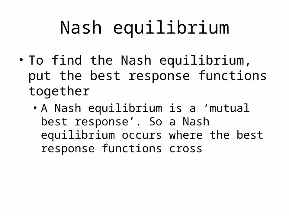
Nash equilibrium
• To find the Nash equilibrium, put the best response functions together• A Nash equilibrium is a ‘mutual best
response’. So a Nash equilibrium occurs where the best response functions cross

Nash equilibriumPlayer 1
Player 20
100
100
The Nash equilibrium is where the best response functions cross. Here it is where both players choose 50. So each player simultaneously and independently choosing ‘50’ is a Nash equilibrium.
50
50

Solving games with continuous strategies
• For each player find their best response function
• Where the best response functions cross, we have a Nash equilibrium

Oligopoly games
• We now want to apply simultaneous games to the behaviour of a small number of firms (an oligopoly)
• Suppose there are just two firms (duopoly)• They produce identical goods. • But each firm must decide how much it will
produce before it goes to sell the product• For example, firms must simultaneously choose
plant size but then given plant size, they will operate at capacity

‘Cournot’ competition in quantities
• Firms simultaneously choose quantities• The market price then adjusts so that the total
quantity produced is sold• Each firm sets its quantity to maximise profits• Note that each firm has a continuous set of
strategies• So we need to calculate each firm’s best response
function (or reaction function)

‘Firm one’s best response function
Output of firm 2
Profit maximising quantity for
firm 1
This is the diagram we need to fill in for firm 1. GIVEN a level of output for firm 2, what is firm 1’s best response?

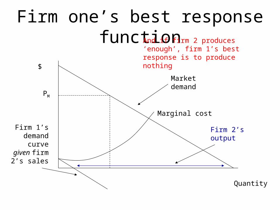
Firm one’s best response function
Quantity
$
Market demand
Marginal revenue
Marginal cost
QM
PM
If firm 2 produces nothing, then the profit maximising best response for firm 1 is to produce the monopoly quantity

Firm one’s best response function
Quantity
$
Market demand
Marginal cost
QM
PM
If firm 2 produces and sells a positive quantity then this reduces the ‘residual’ demand for firm 1.
Firm 2’s output
Firm 1’s demand
curve given firm 2’s sales

Firm one’s best response function
Quantity
$
Market demand
Marginal cost
QM
PM
Firm 2’s output
Marginal revenue GIVEN firm 2’s output

Firm one’s best response function
Quantity
$
Marginal cost
QM
PM
So if firm 2 produces more, the best response for firm 1 is to lower output. Note: firm 1 lowers output by less than firm 2’s increase so overall market price falls.
Firm 2’s output
New optimal quantity
New lower
market price
Firm one’s best response function
Quantity
$
Market demand
Marginal cost
PM
And if firm 2 produces ‘enough’, firm 1’s best response is to produce nothing
Firm 2’s output
Firm 1’s demand
curve given firm 2’s sales

Firm one’s best response function
Output of firm 2
Profit maximising quantity for
firm 1
So we can plot firm 1’s best response function. It starts at the monopoly quantity then falls with a slope less than 1.
Qm
Firm 1’s best response function

‘Cournot’ competition in quantities
Q2
Q1We can do the same for firm 2.
Qm Firm 1’s best response function
Qm
Firm 2’s best response function
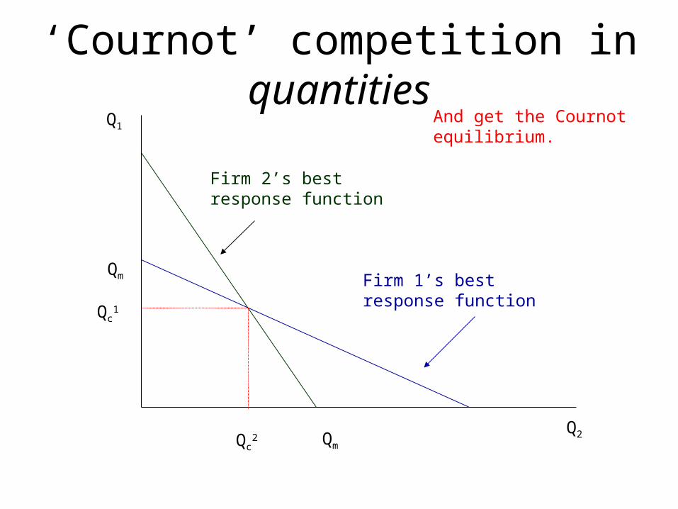
‘Cournot’ competition in quantities
Q2
Q1And get the Cournot equilibrium.
Qm Firm 1’s best response function
Qm
Firm 2’s best response function
Qc2
Qc1

Symmetric firms and ‘Cournot’ competition
Q2
Q1 If the two firms are identical
then Qc1 = Qc
2. Also total
output exceeds the monopoly
quantity.
Qm
Firm 1’s best response function
Qm
Firm 2’s best response function
Qc2
Qc1
45 degree line
(Qm )/2
(Qm )/2
If firm 1’s costs fall then its best response function moves out
• Suppose firm 1’s marginal costs fall but not firm 2’s
• Then for any given output of firm 2, firm 1’s profit maximising output will rise
• So firm 1’s best response function shifts ‘out’ if firm 1’s costs fall

If firm 1’s costs fall then its best response function moves out
Q2
Q1
Qm (original costs)
Firm 1’s new best response function
Qm
Firm 2’s best response function
Qm (new costs)

Firm 1’s costs fall
Q2
Q1
Original Qc2
Original Qc1
New Qc1
New Qc2
So if firm 1’s costs fall, total output rises. Firm 1 produces more in equilibrium and the other firm produces less. Firm 1 makes more profit as (a) its costs are lower and (b) its competitor produces less. Firm 2 makes less profit as (a) total production rises and (b) it produces less. Consumers gain because price falls.

Strategic Substitutes
• Output (or capacity) here is a strategic variable
• Note that the output that is best for one firm falls as the other firm’s capacity increases
• For this reason, we call these type of strategic variables ‘strategic substitutes’.

Summary
• For games with continuous strategies, we model the game by looking at best response functions
• The Cournot competition game has firms simultaneously setting output• The firms produce more than monopoly in
total (but less than perfect competition)• We can capture the strategic effects of a
change in costs for one firm
‘Bertrand’ competition in prices
• Two firms simultaneously choose prices• Consumers then decide which firm to buy from• Each firm sets its own price to maximise profits• As with Cournot competition each firm has a
continuous set of strategies• Here we will consider the case where the two
firms produce imperfect substitutes

‘Bertrand’ competition in prices
• Here we will consider the case where the two firms produce imperfect substitutes• The demand for firm 1 will increase at any price for
firm 1 if the price of firm 2 rises.• The demand for firm 1 will decrease at any price for
firm 1 if the price of firm 2 falls.• And vice-versa for firm 2
We need to find the best response functions (or reaction curves)

‘Firm one’s best response function
Price of firm 2
Profit maximising
price for firm 1
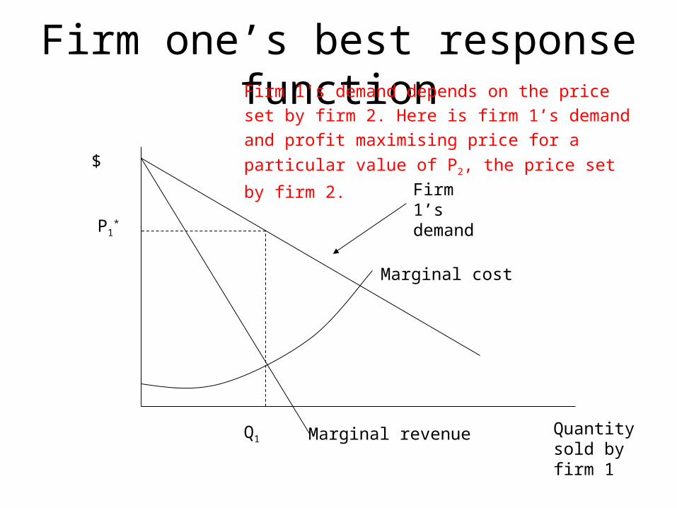
This is the diagram we need to fill in for firm 1. GIVEN a particular price set by firm 2, what is firm 1’s best response?
Firm one’s best response function
Quantity sold by firm 1
$
Firm 1’s demand
Marginal revenue
Marginal cost
Q1
P1*
Firm 1’s demand depends on the price set by firm 2.
Here is firm 1’s demand and profit maximising price
for a particular value of P2, the price set by firm 2.
Firm one’s best response function
Quantity sold by firm 1
$
Marginal cost
Q1
P1*
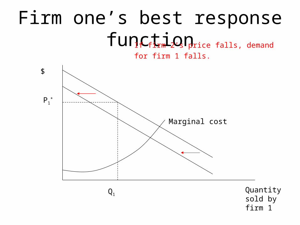
If firm 2’s price falls, demand for firm 1 falls.

Firm one’s best response function
Quantity sold by firm 1
$
Marginal cost
Original P1*
And as a result, the profit maximising price
for firm 1 also falls.
New marginal revenue
New P1*

Firm one’s best response function
Quantity sold by firm 1
$
Marginal cost
Q1
And if firm 2 sets a ridiculously low price (e.g.
gives its product away) then firm 1’s demand
will be very low.
Original P1*

Firm one’s best response function
Quantity sold by firm 1
$
Marginal cost
Q1
In this case, firm 1’s profit maximising price
is also very low – but is still positive.
New P1*
Original P1*
New marginal revenue
Firm one’s best response function
Quantity sold by firm 1
$
Marginal cost Q1
Original P1*
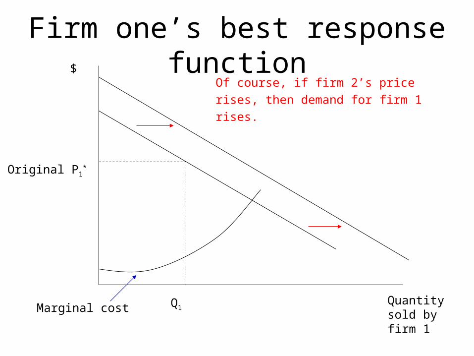
Of course, if firm 2’s price rises, then
demand for firm 1 rises.

Firm one’s best response function
Quantity sold by firm 1
$
Marginal cost Q1
Original P1*
New marginal revenue
New P1*
And in this case firm 1’s profit maximising
price rises.

Firm one’s best response function
• So if firm 2’s price goes up, the profit maximising price for firm 1 goes up
• And if firm 2’s price goes down, the profit maximising price for firm 1 goes down
• So prices are ‘strategic complements’ – they move in the same direction

Firm one’s best response function
Price of firm 2
Profit maximising
price for firm 1
We can plot firm 1’s best response function. It starts at a positive price and slopes up. In general, it also has a slope less than 1 for imperfect substitutes.
Firm 1’s best response function

‘Bertrand’ competition in prices
P2
P1We can do the same for firm 2.
Firm 1’s best response function
Firm 2’s best response function

‘Bertrand’ competition in prices
P2
P1And get the Bertrand price equilibrium
Firm 1’s best response function
Firm 2’s best response function
PB1
PB2

If firm 1’s marginal cost falls …
• Suppose firm 1’s marginal cost falls but not firm 2’s
• Then for any given price of firm 2, firm 1’s profit maximising price will fall
• So firm 1’s best response function shifts ‘down’ if firm 1’s marginal costs fall

If firm 1’s marginal cost falls …
P2
P1
Firm 1’s new best response function with lower marginal cost
Firm 2’s best response function
PB1
PB2

Firm 1’s costs fall
P2
P1
PB1 (original
costs)
PB2 (original costs)
PB1 (new costs)
PB2 (new costs)
If firm 1’s costs fall, both firms lower their prices. Firm 2 makes less profit as its demand has fallen. Firm 1’s profit rises as its marginal costs fall as it is cheaper to make its product. But this benefit is at least partially offset by firm 2 dropping its price.

Strategic analysis of a drop in firm 1’s marginal costs
• Suppose firm 1 can invest in new equipment (a fixed cost) that will reduce its marginal cost. • Under both Cournot and Bertrand consumers win
because prices drop• Under both Cournot and Bertrand, firm 2 loses as firm
1 becomes a stronger competitor. Firm 2 ends up with lower profits and a lower price.
• In both cases firm 1 gains because its marginal costs drop
• BUT – the strategic effect differs
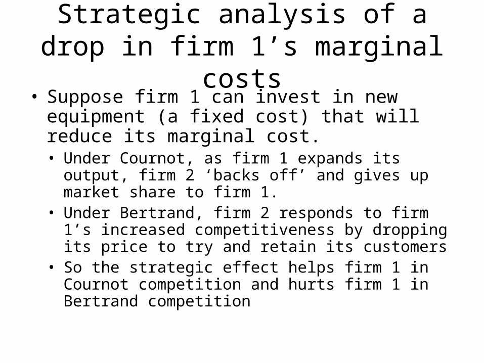
Strategic analysis of a drop in firm 1’s marginal costs
• Suppose firm 1 can invest in new equipment (a fixed cost) that will reduce its marginal cost. • Under Cournot, as firm 1 expands its output, firm 2
‘backs off’ and gives up market share to firm 1.• Under Bertrand, firm 2 responds to firm 1’s increased
competitiveness by dropping its price to try and retain its customers
• So the strategic effect helps firm 1 in Cournot competition and hurts firm 1 in Bertrand competition

Which is correct?
• They both are in the appropriate situations
• To analyse firm behaviour (or any other strategic situations) you need to study the ‘game’ carefully. ‘Small’ changes in strategic interaction can lead to ‘big’ differences in outcomes• (Of course this is why game theory and industrial
economics is interesting)

Summary
• We can capture simple strategic interaction between small numbers of firms (oligopoly) using the Cournot or Bertrand models
• Sometimes these models lead to different predictions – so use wisely
• More generally, when considering strategy, we need to carefully analyse the real world – there are no simple ‘rules’ that always apply.

Reminder: ‘Cournot’ competition in quantities
Q2
Q1
Case of two firms
Qm
Firm 1’s best response function
Qm
Firm 2’s best response function
Q1c
Q2c

Strategy for quantity competition
• If the other firm decreases its output then you can raise your output and increase your profits. • You can do this if you lower your rival’s best
response function. For example if you push up your rival’s costs
• If you can commit to increase your output beyond the equilibrium output then your rival will respond by lowering its output• This raises your profit so long as you do not
increase your output ‘too much’

Reminder: ‘Bertrand’ differentiated goods price competition
P1
P2
Firm one’s best response function
Firm two’s best response function
P1B
P2B
The case of two firms

Strategy for price competition
• If the other firm increases its price then you can raise your price and increase your profits• You can do this by pushing out your rival’s best
response function. For example if you push up your rival’s costs
• If you can commit to increase your price beyond the equilibrium price then your rival will respond by also increasing its price• This raises your profit so long as you do not increase
your price by ‘too much’

So…
• Strategy is all about changing either your best response function or your rival’s best response function• It is about changing the game that you are
playing
• The basic strategic game involves your firm ‘doing something’ before competition between your firm and your rivals

The basic strategy game
Your firm
Choose strategic variable
Both firms
Market interaction: e.g. Cournot or Bertrand competition

But what strategic variables will work?
• For a strategic variable to ‘work’ it must be a credible commitment.• In other words, choosing an action before
competition must affect the actual competition game
• It is not enough to merely threaten and bluster – that is simply cheap talk

Cheap talk in the prisoners’ dilemma
-10, -10 0, -30
-30, 0 -1, -1
Confess
Confess
Don’t Confess
Don’t Confess
Ned
Kelly
Ned Make promise

Ned promises to ‘not confess’. Should Kelly believe him and play ‘don’t confess’? No –
because it pays Ned to cheat.
-10, -10 0, -30
-30, 0 -1, -1
Confess
Confess
Don’t Confess
Don’t Confess
Ned
Kelly
Ned Make promise

Cheap talk
• Just promising to do something or threatening to do something that is not in your own interest is cheap talk.
• To have an effect a strategy must have two requirements• It must be credible – in other words it must be
something you have done and cannot undo easily• It must change the payoffs in the game so that your
rival changes its behaviour in a way that benefits you over all.

Example – commitment to a high price
P1
P2
Firm one’s original best response function
Firm two’s best response function
P1B
P2B
Suppose firm one can commit not to lower its price below P1*
P1*

Example – commitment to a high price
P1
P2
Firm two’s best response function
Firm one’s new best response function
P1*
This commitment by firm 1 leads firm 2 to also raise its price – so both firms make more profit

Example – commitment to a high price
• The commitment to a high price is a ‘soft’ strategy – it raises your rival’s profit as well as your profit
• So it changes the game. But how do we make it credible?• Cannot just ‘promise to raise price’• Can offer a ‘most favoured customer’ agreement to
clients at high price today. This means that if you lower your price in the future, you have to rebate money to all your old customers. It hurts you to drop your price tomorrow – so it is a credible commitment to keep a high price in the future.
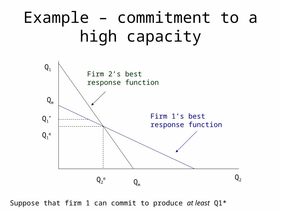
Example – commitment to a high capacity
Q2
Q1
Qm
Firm 1’s best response function
Qm
Firm 2’s best response function
Q1e
Q2e
Q1*
Suppose that firm 1 can commit to produce at least Q1*

Example – commitment to a high quantity
Q2
Q1
Qm
Firm 1’s new best response function
Qm
Firm 2’s best response function
Q1*
This commitment makes firm 2 reduce its output, raising profit for firm 1 and lowering profit for firm 2.

Example – commitment to a high quantity
• This is a ‘tough’ strategy – it raises your profit but reduces your rival’s profit
• So it changes the game. But how do we make it credible?• By building your plant before your rival and• By committing to a large capacity and • By making it difficult to reverse this choice (i.e. difficult to
lower capacity and• if it is difficult to run your plant below capacity, or• if it is cheap to produce output up to plant capacity
• Then you have a credible commitment to produce a high level of output. If your rival observes this commitment then your rival will reduce its plant size, raising your expected profits under competition.
• This is an example of a ‘first mover advantage’

Other examples
• Cortes and burning ships• The ‘pub fight’ from tutorials• International treaties (e.g. the WTO and
protectionism)• Mutually Assured Destruction (MAD) and
the cold war• Reputation (one ongoing player)• ‘Rational’ irrationality

![[ choose any two ]](https://static.fdocuments.in/doc/165x107/617d28e5bae2c57f47187aa6/-choose-any-two-.jpg)