SIMULTANEOUS DESORPTION OF NH3, H2S and C02 FROM AQUEOUS SOLUTIONS

G.C. Hoogendoorn

TR diss 1569

SIMULTANEOUS DESORPTION OF NH3, H2S and COo FROM AQUEOUS SOLUTIONS

SIMULTANEOUS DESORPTION OF NH3, H2S and C02 FROM AQUEOUS SOLUTIONS

PROEFSCHRIFT

ter verkrijging van de graad van doctor aan de Technische Universiteit Delft, op gezag van de Rector Magnificus, Prof.dr. J.M. Dirken, in het openbaar te verdedigen ten overstaan van het College van Dekanen op 29 september 1987 te 16.00 hr

door

Gerardus Cornelis Hoogendoorn

geboren te 's-Gravenhage, scheikundig ingenieur.

TR diss 1569

Dit proefschrift is goedgekeurd door de promotor prof.ir. J.A. Wesselingh

i

STELLINGEN

1. Bij stofoverdracht gevolgd door een instantane chemische reactie hangt de stofoverdrachtssnelheid af van de chemische evenwichten op het gas vloeistof grensvlak. Indien er meer componenten bij betrokken zijn die met elkaar kunnen reageren, dient het gebruik van versnellingsfactoren vermeden te worden. Dit proefschrift Hoofdstuk 2

2. Het begrip schotelrendement heeft geen eenduidige betekenis als de betrokken component in de vloeistoffase een reactie kan ondergaan. Dit proefschrift Hoofdstuk 5

3. Bij beperkte experimentele mogelijkheden zoals die in de praktijk voorkomen, is het experiment waarbij alleen ammoniak uit water wordt gestript het meest effectief om een industriële (sour water) stripper te kunnen beschrijven.

- 4. Een op zich goed artikel waarin voor bekende grootheden afwijkende of niet

suggestieve symbolen worden gekozen, is moeilijk te doorgronden en zal minder geciteerd worden. Hikita H., Konishi Y., 1983, The Absorption Of SO- Into Aqueous Na.CO Solutions Accompanied By The Desorption Of CO.., The Chem. Eng. J., 27, 167-176.

5. Bij het ontwerpen van reactoren en scheidingsapparatuur spelen de evenwichten een belangrijke rol. Toch krijgt zij meestal niet de aandacht die het verdient.

6. Het zou goed zijn als tenminste de familie van chemical engineering tijdschriften dezelfde conventies zou hanteren voor het weergeven van literatuur referenties.

7. De door Zuiderweg voorgestelde methode om stofoverdrachtscoëfficiënten te meten door variatie van de stripfactor is theoretisch correct doch stuit in de praktijk op de beperktheid van het aantal geschikte componenten. Zuiderweg F.J., 1982, SIEVE TRAYS - A View Of The State Of The Art-, Chem. Eng. Sci., 37, 1441-1464.

8. De resultaten van de door Blauwhoff et al. uitgevoerde vergelijking tussen schotel en trickle bed absorbers zijn twijfelachtig omdat hun uitgangsvergelijkingen voor de atmosferische stofoverdrachtscoëfficiënten en fasengrensvlak foutief zijn. Blauwhoff P.M.M., Kamphuis B., van Swaaij W.P.M., Westerterp K.R., 1985, Absorber Design In Sour Natural Gas Treatment Plants: Impact Of Process Variables On Operation And Economics, Chem. Eng. Process., 19, 1-25.

9. Hoewel ons soms anders wordt voorgesteld, correleert de prijs van het aardgas voor kleinverbruikers beter met het begrotingstekort dan met de wereldenergieprijzen

10. Als het niveau van de zeepreklames overeenkomt met die van het aangeprezen product is er nog veel research nodig.

12. Het schrijven van een proefschrift ter verkrijging van de graad van doctor in de technische wetenschappen of een gedichtenbundel zijn twee zeer uiteenlopende zaken; het opdragen ervan aan personen lokt een misplaatste vergelijking uit.

13. De volgende stap in de toekomstige wetgeving voor het veiliger maken van het ongemotoriseerde verkeer zou de invoering van reflecterende hakken kunnen z ij n.

G.C. Hoogendoorn

VOORWOORD

Hierbij wil ik iedereen bedanken die heeft bijdragen bij het tot stand komen van dit proefschrift. Voor het uitvoeren van de experimenten en het opbouwen van de theorie achter dit verhaal moeten de studenten Serge Castel, Zhou Wei Yong, Cyrille Sidawy, Chris Versteegh, Ton Pichel, Theo Driever, Huub van Grieken, Ruben Abellon en Paul Essens genoemd worden. Hun steun en inzet was onontbeerlijk bij het onderzoek. Hans Wesselingh fungeerde als wetenschappelijk geweten en heeft de diverse manuscripten steeds nauwgezet gecorrigeerd. Nu ik de promotieperiode achter de rug heb, zie ik pas goed wat ik allemaal van hem geleerd heb. Aan de medewerkers van het laboratorium voor fysische technologie bied ik nogmaals mijn verontschuldigingen aan voor de overlast die de stripex-perimenten met HpS in het begin gegeven heeft. Gelukkig waren zij bereid ons de tijd te geven om de uitvoering van de experimenten te optimaliseren zodat de voortgang van het onderzoek hierdoor niet belemmerd is. Verder heeft vrijwel iedere medewerker van de vakgroep Chemische Technologie (of het instituut) op zijn vakgebied iets bijgedragen aan het onderzoek. Ook hen wil ik bedanken voor de plezierige samenwerking die ik de afgelopen jaren heb ondervonden.

CONTENTS

Chapter 1 Introduction 1

Chapter 2 Theory And Experiments On The Simultaneous Desorption Of Volatile Electrolytes In A Wetted Wall Column. - Ammonia And Hydrogen Sulphide Desorption-Abstract 5 1. Introduction 5 2. Theory 7 2.1. Wetted Wall Column 7 2.1.1. Liquid Hydrodynamics 7 2.1.2. Gas Hydrodynamics 9 2.2. Desorption With Chemical Reaction 9 3. Experimental 13 3.1. Description Of The Column 13 3.2. Flow scheme 11 1. Results 15 1.1. Computer Simulations 15 1.2. Experiments 20 5. Conclusion 21 6. Symbols 25 7. Literature 26

Chapter 3 Theory And Experiments On The Simultaneous Desorption Of Volatile Electrolytes In A Wetted Wall Column. - Ammonia And Carbon Dioxide Desorption-Abstract 28 1 . Introduction 28 2. Theory 29 2.1. Desorption With Chemical Reaction 29 3. Results 32 3.1. Computer Simulations 32 3.2. Development Of A Simple Model 35 3.3. Experiments 11

Samenvatting 109 Appendix 1 Mass Transfer Parameters 1. Summary Of Literature Correlations A-11 1.1. Liquid Mass Transfer Coefficient k A-1 1.2. Gas Mass Transfer Coefficient k A-2

8 1.3. Interfacial Area a A-2 1.1. Volumetric Liquid Mass Transfer Coefficient k a A-3 1.5. Volumetric Gas Mass Transfer Coefficient k.a A-3 2. Experimental A-1) 2 . 1 . Theory of Danckwerts method A-1

2 . 2 . E q u i l i b r i u m Data A-6

3 . R e s u l t s A-6

3.1. Wetted Wall Column A-6 3.2. Measurements On A Single Tray At Room Temperature A-7 3.3- Measurement Of The Interfacial Area At 103 °C A-8 3.1. Measurement Of The Gas Mass Transfer Coefficient

At 103 °C A-10 3.5. Comparison With Literature A-11 1. Conclusion A-1 3 5. Symbols A-11 6. Literature A-15

Appendix 2 Experience With An Optical Probe For Measuring Bubble Sizes And Velocities On A Sieve Tray 1. Introduction A-17 2. Principle A-17 3. R e s u l t s And Discuss ion A-20

1. Conc lus ion A-23

5. Symbols A-21

6. Literature A-21

Appendix 3 Listing Of Stripping Program From Chapter 5 A-25

5. Conclus ion 146

6. Symbols 17

7. Li terature 1J8

Chapter 1 Theory And Experiments On The Simultaneous Desorption Of Volatile Electrolytes In A Wetted Wall Column. - Ammonia Hydrogen Sulphide And Carbon Dioxide Desorption-Abstract 19 1. Introduction 19 2. Results 51 2.1. Desorption With Chemical Reaction 51 2.2. Experiments 53 3. Conclusion 55

Chapter 5 Desorption Of Volatile Electrolytes In A Tray Column (Sour Water Stripping) Abstract 56 1. Introduction 56 2. Basic Data 57 2.1. Vapour Liquid Equilibria 57 2.2. Mass Transfer Coefficients (Literature Review) 61 2.3. Mass Transfer With Chemical Reaction 68 3. Model 73 1. Experimental Procedures 75 1.1. Equipment 75 1.2. Analytical Methods 77 5. Column Hydrodynamics 78 6. Experimental And Simulated Results 79 7. Comparison Between Predicted And Reported Performance 87 8. Stage Efficiencies 92 8.1. Murphree Efficiency 92 8.2. Vaporization Efficiency 96 9. Conclusion 101 10. Symbols 103 11 . Literature 106

Summary 108

CHAPTER 1

INTRODUCTION

Desorption and absorption processes are commonly encountered in the chemical industry. This thesis is a comprehensive study of the simultaneous desorp­tion of volatile weak electrolytes such as ammonia, hydrogen sulphide, carbon dioxide and phenol from aqueous wastes. The removal operation, generally known as sour water stripping, is done in tray or packed columns. In practice steam is used as a stripping agent. It forms an important part of integrated industrial aqueous waste management. The process is of sufficient importance to have given rise to a number of publications. These can be divided in two main groups:

- studies of the vapour liquid equilibria of the solutions and - summaries of operating and engineering experience.

The first category is well developed. Already in 1919 van Krevelen et al. published an article called "Composition And Vapour Pressures Of Aqeous Solutions Of Ammonia, Carbon Dioxide And Hydrogen Sulphide". Several others followed. When Maurer (1980) published "On The Solubility Of Volatile Weak Electrolytes In Aqueous Solutions", the description of the equilibria seems to be complete. A good example from the second category is the paper by Beychok's (1968). "The design of sour water strippers" deals with tray to tray calculations based on the equilibria from the pioneering work of van Krevelen et al.. In later publications (Walker 1969, Boberger and Smith, 1977) deviations from equilibrium behaviour have been reported and taken account by column or tray efficiencies. Won (1983) has furthur extended this approach. He has derived component efficiencies from operating data an industrial strippers. These data were collected by the American Petroleum Institute (1973). Won's approach is regarded as the best current procedure and has already found its way into 'The Chemical Engineers Handbook' Perry (1984). With so much background available one might wonder "why furthur research on sour water stripping ?". The answer can be found in Won's article of which we quote: "A basic mathematical description of a real stage can be made by incorporating mass and heat transfers and ionic reaction rates as well as fluid dynamics. In general, the lack of fundamental knowledge of fluid

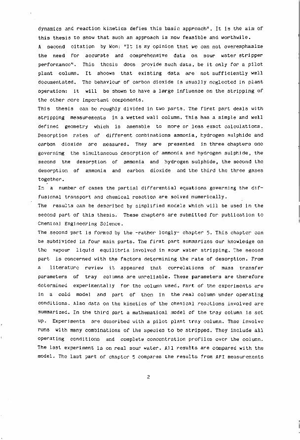
dynamics and reaction kinetics defies this basic approach". It is the aim of this thesis to show that such an approach is now feasible and worthwile. A second citation by Won: "It is my opinion that we can not overemphasize the need for accurate and comprehensive data on sour water stripper performance". This thesis does provide such data, be it only for a pilot plant column. It shoows that existing data are not sufficiently well documentated. The behaviour of carbon dioxide is usually neglected in plant operation: it will be shown to have a large influence on the stripping of the other more important components. This thesis can be roughly divided in two parts. The first part deals with stripping measurements in a wetted wall column. This has a simple and well defined geometry which is amenable to more or less exact calculations. Desorption rates of different combinations ammonia, hydrogen sulphide and carbon dioxide are measured. They are presented in three chapters one governing the simultaneous desorption of ammonia and hydrogen sulphide, the second the desorption of ammonia and hydrogen sulphide, the second the desorption of ammonia and carbon dioxide and the third the three gases together. In a number of cases the partial differential equations governing the dif-fusional transport and chemical reaction are solved numerically. The results can be described by simplified models which will be used in the second part of this thesis. These chapters are submitted for publication to Chemical Engineering Science. The second part is formed by the -rather longly- chapter 5. This chapter can be subdivided in four main parts. The first part summarizes our knowledge on the vapour liquid equilibria involved in sour water stripping. The second part is concerned with the factors determining the rate of desorption. From a literature review it appeared that correlations of mass transfer parameters of tray columns are unreliable. These parameters are therefore determined experimentally for the column used. Part of the experiments are in a cold model and part of them in the real column under operating conditions. Also data on the kinetics of the chemical reactions involved are summarized. In the third part a mathematical model of the tray column is set up. Experiments are described with a pilot plant tray column. Thse involve runs with many combinations of the species to be stripped. They include all operating conditions and complete concentration profiles over the column. The last experiment is on real sour water. All results are compared with the model. The last part of chapter 5 compares the results from API measurements

2

on industrial columns with the model developed. It also discusses the pos­sibility of simplifying the model by the use of different kinds of tray efficiencies. Chapters 2, 3 and H have submitted for publication in "Chemical Engineering Science". Chapter 5 has been submitted for publication to "Chemical Engineering Research and Design". Because these are seperate articles there is some overlap between them, for which I offer my excuses.

LITERATURE

American Petroleum Institute, 1973, 1972 Sour Water Stripping Survey Evaluation, Publication No. 927, Washington D.C., 6lp. Beychok M.R., 1968, The Design Of Sour water Strippers, Proceedings of the Seventh World Petroleum Congres, 9, Elsevier Barking, 313-332. Bomberger D.C., Smith J.H., 1977, Use Caustic To Remove Fixed Ammonia, Hydrocarbon Processing, 56, 157-162. Krevelen van D.W., Hoftijzer P.J., Huntjens F.J., 19^9, Composition And Vapour Pressures Of Aqueous Solutions Of Ammmonia, Carbon Dioxide And Hydrogen Sulphide, Recueil, 68, 191-216.

Maurer C , 1980, On The Solubility Of Volatile Weak Electrolytes In Aqueous Solutions, Thermodynamics Of Aqueous Systems With Industrial Applications, ACS Symposium Series 133, American Chemical Society, Washington D.C., 139-172. Perry R.H., Green D.W., 1981, Chemical Engineer's Handbook, Sixth Ed., Mc Graw Hill New York, 13-53. Walker G.J., 1969, Design Sour Water Strippers Quickly, Hydrocarbon Processing, 18, 121-12U.

Won K.W., 1983, Sour Water Stripping Efficiency, Plant/Operations Progress, 2,108-113.

3

CHAPTER 2

THEORY AND EXPERIMENTS ON THE SIMULTANEOUS DESORPTION OF VOLATILE ELECTROLYTES IN A WETTED WALL COLUMN

- AMMONIA AND HYDROGEN SULPHIDE DESORPTION -

G.C. Hoogendoorn, J.A. Wesselingh, S.D.L. Castel Delft University of Technology Department of Chemical Engineering Julianalaan 136 2628 BL Delft The Netherlands

ABSTRACT

Complete numerical solutions are presented of the simultaneous desorption of NH, and H S at a stagnant water gas interface. These include the transport and reactions of all the major ionic species involved. It is also shown that the same results can be predicted using a much simpler model. The theories are substantiated by desorption experiments at HO °C in a cocurrent wetted wall column.

1 . INTRODUCTION

Desorption of ammonia and hydrogen sulphide from water is commonly encountered in industrial practice. Such water commonly arises from the washing of reaction products that have been treated in hydrodesulfurization or hydrocracking operations. This kind of water is commonly called sour water, although its pH value is usually somewhat basic. Removal of the sulphides is essential to meet effluent regulations or to reuse the water. This removal is usually done by steam stripping in tray or packed columns. The mechanism of the desorption process is not as well understood as that of the analogous absorption processes. The American Petroleum Institute (1973) had arranged a survey on sour water stripping practice. One of their final conclusions is that more fundamental information on the desorption should be

5

obtained and integrated in the design of sour water strippers. Until now strippers are still designed by tray to tray equilibrium calculations (Wild, 1979), although there is strong evidence that kinetics play an important role (Darton et al. 1978). According to the API report sour water contains about 3000 ppm ammonia and 3*)00 ppm hydrogen sulphide. In practice other contaminants such as phenolics, cyanides, acids or bases, oil and carbon dioxide are present. In this study however they will not be taken into account. The theory of absorption of a gas into a liquid where it undergoes a chemi­cal reaction is well understood and treated extensively in literature. The basic theory is treated well in the books of Danckwerts (1975) and Astarita (1967). For more difficult reaction schemes review articles such as published by Ramachandran and Sharma (1971) can give insight. Experiments and theory on the selective absorption of carbon dioxide and hydrogen sul­phide from sour gases in alkanolamine solutions have been reported recently by Blauwhoff (1982). Desorption has attracted much less attention. Shah and Sharma (1976) published a review article about desorption, Astarita and Savage (1980) presented a theoretical analysis of desorption, and using this theory, Savage et al. (1980) presented measurements for the desorption of carb­ondioxide from hot carbonate solutions. Mahajani and Danckwerts (1983) have measured desorption rates of carbondioxide from potash solutions with and without the addition of amines. At first sight absorption and desorption are comparable operations, because the governing equations are the same. However the differences are larger than "a change in the sign of the driving force" as suggested by Danckwerts (1975).

- Reversibility of the chemical reactions should be taken into account for a desorption process. The equations derived for an absorption followed by an irreversible reaction cannot be applied to desorption processes.

- In absorption the gas phase resistance can be eliminated by working with a pure gas. This was done by e.g. Astarita and Gioia (1961). This is not possible for a desorption process.

- The solute concentration in reactive media in the bulk of the liquid is usually low. So the driving force for mass transfer for an absorption is

6

equal to the interfacial concentration of the solute. In desorption however this small bulk concentration is the main factor in the driving force and cannot be neglected. As a consequence an accurate knowledge of the chemical equilibria in the liquid phase is required.

- For absorption the ratio between the interfacial and the bulk concentra­tion can have any value between one and infinity. For desorption however this ratio is between zero and one. So the possible range of driving forces is much larger for absorption. This was already remarked by Astarita and Savage (1980).

2. THEORY

2.1. WETTED WALL COLUMN

A wetted wall column is an apparatus widely used for studying mass transfer phenomena. It has the advantage of a known exchange area between gas and liquid and simple hydrodynamics, so important parameters such as interfacial area and liquid and gas phase mass transfer coefficients are known. Therefore it was decided to study simultaneous desorption of ammonia and hydrogen sulphide in a wetted wall column.

2.1.1. Liquid Hydrodynamics

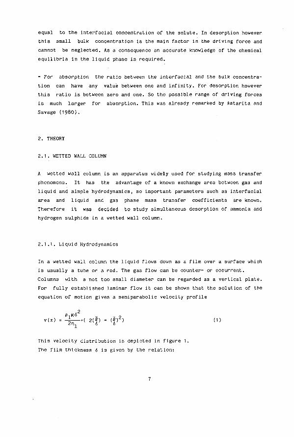
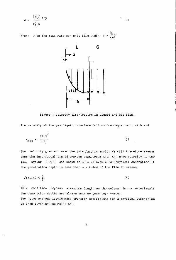
In a wetted wall column the liquid flows down as a film over a surface which is usually a tube or a rod. The gas flow can be counter- or cocurrent. Columns with a not too small diameter can be regarded as a vertical plate. For fully established laminar flow it can be shown that the solution of the equation of motion gives a semiparabolic velocity profile

p l g 6 z z 2 v(z) = -i- ( 2(f) - (fr) (1)

This velocity distribution is depicted in figure 1. The film thickness 6 is given by the relation:

7

(IV\l/3 v 2

P l g

(2)

Where r i s the mass ra te per unit film width: r Vl n-d

Figure 1 Velocity distribution in liquid and gas film.

The velocity at the gas liquid interface follows from equation 1 with z=6

,2 gpx6 (3)

The velocity gradient near the interface is small. We will therefore assume that the interfacial liquid travels downstream with the same velocity as the gas. Nysing (1957) has shown this is allowable for physical absorption if the penetration depth is less than one third of the film thickness

/(nD1t) < | (1)

This condition imposes a maximum length on the column. In our experiments the desorption depths are always smaller than this value. The time average liquid mass transfer coefficient for a physical desorption is then given by the relation :

k. = 2-A-i) (5) 1 0 TTt

The flow pattern in the liquid film depends on the Reynolds number which is usually defined as :

Re, - M (6) 1 nx

It has been found that the transition from laminar to turbulent flow occurs at a Reynolds number of about 1200 (Emmert et al. 1951) or 1600 (Brauer, 1971). A value of 280 is used in this work.

2.1.2 Gas Hydrodynamics

In the situation chosen here, the gas has a velocity equal to the interfa-oial velocity of the liquid (see figure 1). The gas flows through the column without velocity gradients. This results in zero shear and zero pressure gradient over the column. This choice is the same as used by Berg and Hoornstra (1977) and Lefers (1980). The Reynolds number for the gas phase, taken as pvd/n, is about 610 in this work. Provided the Graetz number for the gas is high, the gas phase can be con­sidered as infinitely deep and this situation corresponds to the penetration theory solution for the mass transfer coefficient for physical ab- or desorption.

k" = 2 ••(-£-) (7) go ir.t

2.2. DESORPTION WITH CHEMICAL REACTION

Mass transfer in the solutions considered is governed by a number of dif­ferential equations. These are definied by the mass balances of the transferring components. The mass balance for a component i can be written as

3C at1 = "VJi + ri (8)

which states that the accumulation of a species i in a differential element is equal to the net input (in three directions) due to flow and the net production of a homogeneous chemical reaction. For expressing the flux equation we have considered here the Nernst Planck equations describing diffusion in ionic solutions (Sherwood and Wei, 1955). It turned out that the electrical effects included in these equations were unimportant, because the diffusion coefficients of the components are almost equal. Therefore Fick's law can be used for expressing the flux equation

J. = -D.vC. + v-C. (9)

Applying stationary conditions to the column as a whole, the mass balance reads

0 = D.72C. - V(vC. ) + r. (10)

Neglecting the diffusion in vertical direction and taking into account only a velocity in vertical direction, equation (10) can be written for the wetted wall column as

32C 3C. 0 = D. Trpr- " v -i + r, (11)

1 dz dh 1

or with t = - , one obtains v

3C. 32C. ^r 1 = D. ^-yi + r. (12) 3t l 3z l

This equation describes the evolution of the concentration of component i in an element as a function of its time in the column and the penetration depth. The production term r. which is a function of the concentrations, couples the equations of the different components. For the gas phase similar equations can be written without the reaction term. When ammonia and hydrogen sulphide are dissolved in water the following compounds exist:

H20, NH , H2S, NH*. HS", 0H_, H+, S2".

10

The concentration of each individual species in the liquid and gas phase at equilibrium for given total concentration of ammonia N and hydrogen sul­phide S can be calculated with the procedure and data (dissociation and Henry's constants, equations for activity coefficients) of Edwards et al.(1978). On molar basis a sour water contains more ammonia than hydrogen sulphide, so

+ 2-in the alkaline solutions of the weak base NH , H and S can be neglected. The main reactions to be considered are:

k1 NH. + H O ■«- » NH. + OH (13) 3 d K , H -1

-2 H2S + OH ■«ƒ » HS + H20 (11)

For the components NH , U S , NH. and HS a set of equations (12) can be written, the OH concentration can be calculated from the electroneutrality relation

[OH ] = [NH,,] - [HS ] (15)

These equations can be integrated numerically from time equals zero up to the contact time and from distance equals zero up to the film thickness. The initial conditions for the liquid phase are t = 0 , for all values of z:

[NH3] = CNH3]b ; [NH*] = [NH*]b ; [H^] = C H2S ] b < £HS~] = ^HS~^b

(16) The boundary conditions at the gas liquid interface are

for the molecular forms NH and H S

[NH ] [H S] [NH,]. = i-6 a n d [H.S], = -B (17)

3 1 mNH3 2 l mH2S

with m the partition coefficient in appropriate units for the non volatile ions at the interface

11

d[HS 3 = d[NHJ = dz ~~ dz (18)

Boundary conditions in the bulk of the liquid are

C. = C. . n, for all components l i.bulk y (19)

The gas phase differential equations have similar boundary conditions.

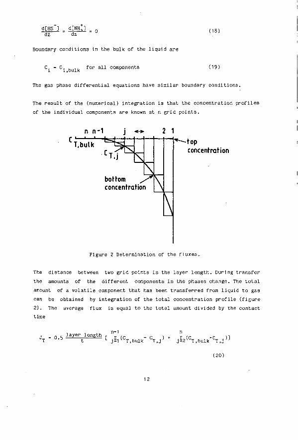
The result of the (numerical) integration is that the concentration profiles of the individual components are known at n grid points.

bottom concentration

-top concentration

Figure 2 Determination of the fluxes.

The distance between two grid points is the layer length. During transfer the amounts of the different components in the phases change. The total amount of a volatile component that has been transferred from liquid to gas can be obtained by integration of the total concentration profile (figure 2). The average flux is equal to the total amount divided by the contact time

_ layer length r n"1 . . JT U'b t L jil(CT,bulk S . j ' j=2(CT,bulk"CT,j)]

(20)

12

These liquid fluxes should equal the gas fluxes which can also be determined with equation 20. Equality can be obtained by changing the values of the concentration in equation 17. With this procedure the fluxes were calculated numerically for a given composition N , S .

3. EXPERIMENTAL

3.1. DESCRIPTION OF THE COLUMN

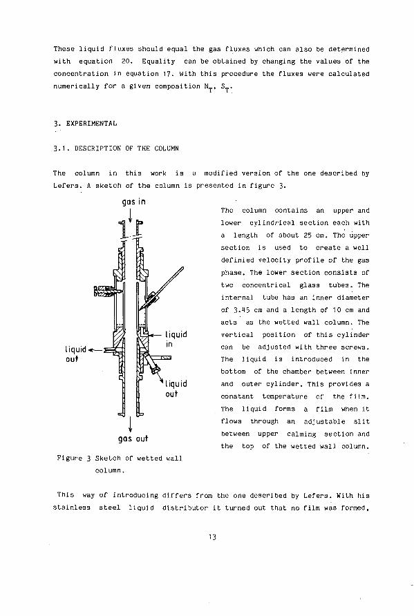
The column in this work is a modified version of the one described by Lefers. A sketch of the column is presented in figure 3.

The column contains an upper and lower cylindrical section each with a length of about 25 cm. The upper section is used to create a well definied velocity profile of the gas phase. The lower section consists of two concentrical glass tubes. The internal tube has an inner diameter of 3. 5 cm and a length of 10 cm and acts as the wetted wall column. The vertical position of this cylinder can be adjusted with three screws. The liquid is introduced in the bottom of the chamber between inner and outer cylinder. This provides a constant temperature of the film. The liquid forms a film when it flows through an adjustable slit between upper calming section and the top of the wetted wall column.

liquid-out

liquid out

gas out

Figure 3 Sketch of wetted wall column.

This way of introducing d i f fers from the one described by Lefers. With his s t a in l e s s s t e e l l iquid d i s t r ibu to r i t turned out that no film was formed,

13

due to the bad wettability of steel, but that the liquid flowed down in a number of channels. The film covering the inner surface of the tube flows down and is removed through another slit into an annular pool with a small surface area. In this way the gas is separated from the liquid. The liquid level in the pool is controlled. The air also flows downwards through the column. The tempera­tures of gas and liquid could be measured by means of thermometers.

3.2. FLOW SCHEME

The equipment is shown in figure 4.

*"»

1. GAS CYLINDER 2. FEED PREPARATION 3. CONSTANT TEMP. VESSEL 1». PUMP 5. FLOWMETER 6. WETTED WALL COLUMN 7. HUMIDIFIER 8. C02 ABSORBER

air in 9. SAMPLING POINT

Figure 4 Flow scheme.

The solution for stripping is prepared in vessel 2. An amount of water (about 2.5 1) is added to and heated in the vessel. When the operating temperature is reached, an amount of 33% ammonia solution (Merck) is added to the water. Then the hydrogen sulphide (Matheson) from a gas cylinder is introduced under stirring in the vessel and absorbed in the ammonia solution. The solution is led to vessel 3. A pump cycles the contents of this vessel through the stripping column. In the course of time (over several hours) the concentrations in vessel 3 gradually change. They are regularly monitored to determine the desorption fluxes. The total liquid volume in the system is about 2 1. Two experimental details are worth

14

mentioning. Ammonia and hydrogen sulphide are both very volatile and easily lost. It is therefore absolutely necessary to minimize the (dead) gas volumes in the circulation loop. Also the use of plastic tubes has to be minimized as these materials are quite permeable for the gases studied. The air flows through a meter, bubbles through a 5 M sodium hydroxide solu­tion to remove carbon dioxiode and is saturated with water at the operating termperature in the humidifier 7 to prevent transfer of water in the column. After stripping the air leaves the bottom of the column and is removed by means of suction. The column itself is mounted on a heavy table and installed with flexible connections between the column and the rest of the equipment. This is done because the film proved to be very sensitive to vibrations. These (small) vibrations, originating from e.g. a pump or suction device, are immediately visible as waves on the surface of the film. These waves might enhance mass transfer. Waviness was reduced to an invisible extent by addition of 0.025 vol % of Teepol as described by Lynn et al.(1955). This addition also prevented the film from breaking up into channels. As Teepol is absolutely necessary for obtaining a film, no experiments were carried out to study its influence on the mass transfer.

4. RESULTS

4.1. COMPUTER SIMULATIONS

To demonstrate the behaviour of the NH -H_S desorption, simulations were done for a constant-total ammonia concentration in the bulk of the liquid N = 0.0882 mol»kg .. The total sulphur concentration S„ was varied from 0.0882 mol-kg . to 0.00882 mol-kg , giving molar ratio's R = N T / S T fr°rn 1 to 10. Values of relevant physical and chemical parameters were taken at 10 °C. Diffusion coefficients were calculated from Perry (1982). For NH. and H S in the gas phase the Wilke Lee equation was used, for the liquid phase the Wilke and Chang equation was taken. The ion diffusion coefficients have been calculated with the Nernst equation. The values of k

A O — 1 — 1 ' 7 0 — 1 — 1 ' (1-10 m «mol -s ) and k {1 -10 m -mol . »s ) were taken from Eigen et al. (1961) and corrected for the temperature difference.

15

LL = 1.7-10"4m LQ =1.7»10"2m t=0.33s

• NH3 xH2S o OH" A NH*4HS"

NT =0,0882 ^

* - * ■ * *

o-<X>

mol ST=0.0882 ST = 0,02206 ST =0,00882 ^

L \ G L G L G

A—A-6-^

O—OoA x

X — X-X->

X *

LL 00 LG LL 00 LG LL 00 LQ

< > distance

Figure 5 Calculated concentration profiles in liquid and gas films as function of the composition.

16

Figure 5 gives the concentrations of all relevant species as a function of the position in the film for R values of 1, H and 10. It should be remarked that the horizontal scale in the gas phase (L_) is 100 times larger than

u that of the liquid phase (L ). In figure 6 the total fluxes of NH and H,S

L 3 2 are represented as a function of the composition. The following conclusions can be drawn from the calculations and figures.

- The NH. and HS profiles are almost the same. This effect is caused by the electroneutrality relation. In figure 5 the ions are represented as a single component.

Everywhere in the liquid film , so from bulk to interface, the ratios [NH ] [H2S][0H]

and rrrr;—i— remain constant. K][0H-] an [HS-J

This means that reactions 13 and ^H can be regarded as instantaneous.

-The interfacial concentrations of all components are the same at all heights.

- With lower total sulphur concentrations the profiles of the components H„S and HS become flatter. This means that mass transfer for H S becomes more gas phase controlled.

- Higher concentrations of total sulphur have a remarkable effect on the NH, profile. It causes a flattening of the profile. In the left side of figure 5 this effect has even resulted in an increasing concentration of NH towards the the interface. This does not mean that ammonia is absorbed; there is

+ still a net flux of ammonia towards the gas phase, caused by the NH. ion. This effect is a result of the coupling, via the OH ion, of the two simul­taneous desorption processes and becomes more pronounced at higher sulphur concentrations. To explain this effect it should be kept in mind that NH is 120 times more soluble than H_S. So H.S will desorb rapidly, thereby lower­ing the concentration of HS . A lower concentration of HS will (because of

+ electroneutrality) lower the concentration of NH., which can only be achieved if reaction 13 proceeds from right to left. A part of the NH, amount that is produced by this reaction, will diffuse back into the bulk of the liquid.

17

- From figure 6 it is clear that the composition, and so the degree of ionization, has a large effect on the fluxes. This is not only due to a change in equilibrium gas phase concentrations but also to mass transfer aspects.

- To bring into account the acceleration of an ab- or desorption by a chemi­cal reaction, the enhancement factor concept is widely used. A commonly used definition of the enhancement factor of ammonia can be given as

total flux of ammonia with chemical reaction N = flux of ammonia alone under the same driving force

and an analogous definition of the factor of hydrogen sulphide E . Values from the simulations are given in table 1. The enhancement factor of ammonia shows a remarkable dependancy on the concentrations. It can be noticed that the enhancement factor becomes negative for high sulphur con­centrations, and at R = 2.2 an asymptote can be calculated. The explanation of this phenomenon can be found in the form of the concentration profile and the the definition of the enhancement factor. For absorption the negative enhancement factor has also been observed by Cornelisse et al. (1980) and in Blauwhoff's thesis for what they call 'forced desorption'. The cause of the negative enhancement factor is the same for both absorption and desorption: a strong influence of another component. The concentration profiles differ fundamentally. In the absorp­tion case, on basis of a positive (= absorption) overall driving force, desorption was found. For the desorption case, on basis of a. positive (= desorption) overall driving force, desorption is found. This does make us wonder wether the concept is of much use in these more complicated situations in the instantaneous reaction regime.

- From the behaviour of the complete equations it can be seen that the fluxes can be predicted by the following equations.

JNH 3 = kl,NH3

Pl ( [NH3]l,b " CNH33l,int) + kl,NH, Pl( [ K ] b " K]lnt>

" kl Pl( Y b " Y i n ^ (21)

■ kg,NH3 V CNH3]g.mt - ^ V g . b ' ( 2 2 )

19

JH 2S " k l , H 2 S p l ( [ H 2 S ] l , b " ^ l . i n t ' + k1 > H S - P l ( C H S " ] b " ^ i n t '

" k l p l ( S T,b " ^ . i n t 5 ( 2 3 )

= k „ q p ( [H-Si - CH,S]„ . ) (21) g,H2S rg 2 g.int 2 g,b

with

C N f U „ , „ t " V L E ( N T . S T ) . . and [H.Sl = VLE (N_,S_) . . 3 g , m t T T i n t 2 g , m t T T i n t

(25 )

where VLE is the set of Vapor Liquid Equilibrium relations for the compounds. The equations 21 to 25 can be solved for the two unknowns N . and S . , giving the same results for the fluxes as the numerical method. Notice that the VLE relations only have to be applied to calculate the compositions at the interface. In equations 21 and 23 it is assumed that all the components have the same mass transfer coefficient, which is not un­reasonable because the diffusion coefficients have almost the same value.

1.2. EXPERIMENTS

Desorption experiments on the wetted wall column were done at a temperature of 10 °C. The experiments yield curves of concentration versus time, which can be converted to fluxes according to :

V ^ T T a dt

where V is the volume of the system, and a the gas liquid exchange area. First the liquid and gas phase hydrodynamics were checked by measuring the desorption rate of NH alone (gas phase controlled) and H S alone (liquid phase controlled) from water. Out of these experiments values for the mass transfer coefficients were calculated that were within 3% of the theoretical values calculated with equations 5 and 7. Because of this good agreement no attempts were undertaken to determine the length of the stagnant zone near

20

t/l «NI

e o E

-4-O

10

: measured

x , • : computed

- x _ v H 2 *

_l I I . I l_ 4000 8000

»— time (sec) 12000

Figure 7 Measured and calculated fluxes for experiment 1.

CM E

o E

O

x x

20

10

measured

x , • : computed

J I I L 1000 2000 3000 4000 5000 6000

— ■ time (sec)

Figure 8 Measured and calculated fluxes for experiment 2.

21

the liquid outlet which would not be active in the physical desorption (Lefers). Three experiments with NH and H S were performed wi th d i f f e r e n t i n i t i a l

c o n c e n t r a t i o n s :

Experiment 1

Experiment 2

Experiment 3

NT = 0.1114 mol-kg

N = 0.081 mol-kg"

N = 0.078 mol-kg -1

ST = 0.035 mol-kg

S = 0.063 mol-kg

S_ = 0.093 mol-kg"

and o t h e r ope ra t i ng c o n d i t i o n s held c o n s t a n t :

(j> . = 5-10~ 3 k g - s " 1 , <j> = 3.31 -10~H k g - s " 1 , a = 1 . 2 - 1 0 " 2 m 2 , L = 0.11 m.

t-L = T = -33 s , 6 = 0.21 mm, T = 10 °C.

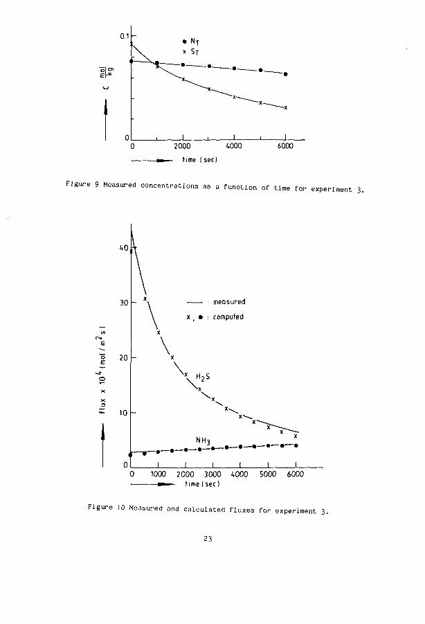
The results of the measurements are given in figure 7 to 10. In an experi­ment the concentrations become lower and so do the fluxes (experiment 1). For experiment 2 and 3 it is observed that the ammonia flux increases in time. The total concentration of ammonia decreases in time ( figure 9 ). As a result of the high initial sulphur concentrations in experiment 2 and 3 J, + .. „ has a high value. This results in a liberation of NH, from NH„HS at a n2o 3 4 rate which is higher then the flux of ammonia to the gas. The net effect is therefore a decreasing N with an increasing [NH ], which is favourable for a higher ammonia flux. The experimental fluxes, represented as the continuous lines, are compared with the theoretical values of the fluxes calculated with equations 21 to 25. The agreement is seen to be excellent.

22

p IF

2000 WOO time ( sec)

6000

Figure 9 Measured concentrations as a function of time for experiment

: measured x _ • : computed

o E

k — •—• •

1 .. I I L 0 1000 2000 3000 4000 5000 6000

m time(sec)

Figure 10 Measured and calculated fluxes for experiment 3.

23

5. CONCLUSION

Rates of desorption of ammonia and hydrogen sulphide from solutions can be predicted with a relative simple model, because the reactions are instantaneous. The theories and model presented take the liquid as well as the gas phase resistance to mass transfer into account. From numerical simulations followed that at higher concentrations of total sulphur the enhancement factor for ammonia becomes negative, while the ammonia flux is still towards the gas phase. In this case ammonia is desorbed with an in­creasing concentration profile towards the interface. Model calculations for the fluxes agree well with measurements on a wetted wall column. All measurements were carried out at a temperature of 10 °C. The model presented can be applied to any type of desorption equipment provided that k.a and k a are known.

21)

6. SÏBOLS

a

C

E

g h

J

k. ï k,

i n t e r fac ia l area concentration enhancement factor accelerat ion of gravity coordinate flux mass t ransfer coefficient react ion ra te constant

length

partition coefficient

R concentration ratio N /S r. production rate Re Reynolds number N total NH concentration S total H S concentration v velocity V volume z coordinate

Greek

r 6

ri

m P T

V

subs

b

g i

c r i

mass r a t e per unit film width filmthickness v iscos i ty mass flow density residence time nabla operator

pt

bulk gas

component i

2 m mol

m-s

m

mol

m-s

m T

-1 s . IT)

mol

mol (-) mol

(-) mol

mol

m's

m3

. -1 •kg

-2

2 • •m -s -1

-1 nol

•kg'1

, -1 •kg

-3 •m •;

•kg'1

•kg"1

-1

-1

-1 •s .

gas

liqu

r1

or

lid

-1 -1 kg Tn >s .

N -s -m kg-s

-3 kg-m

25

int interface 1 liquid T total 0 physical

7. LITERATURE

American Petroleum Institute, 1973, Sour Water Stripping Survey Evaluation, Report WBWC 3061, Publication No 927, Washington D.C. Astarita G., 1967, Mass Transfer With Chemical Reaction, Elsevier.Amsterdam. Astarita G., Gioia F., 1961, Hydrogen Sulpide Chemical Absorption, Chem.Eng.Sci., 19, 963-971.

Astarita G., Savage D.W., 1980, Theory Of Chemical Desorption, Chem.Eng.Sci., 35, 649-656. Berg H. van den, Hoornstra R., 1977, The Distribution Of Gas-Side And Liquid- Side Resistance In The Absorption Of Chlorine Into Benzene In A Wetted Wall Column, Chem.Eng.J., 13, 191-200. Blauwhoff P.M.M., 1982, Selective Absorption Of Hydrogen Sulphide From Sour Gases By Alkanol Amine Solutions, Ph.D.Thesis, Twenthe University.

Brauer H., 1971, Grundlagen Der Einphasen Und Mehrphasenstromungen, Sauerlander AC, Aarau. Cornelisse R., Beenackers A.A.CM., Beckum van F.P.H., Swaaij van W.P.M., 1980, Numerical Calculations Of Simultaneous Mass Transfer Of Two Gases Accompanied By Complex Reversible Reactions, Chem.Eng.Sci., 35, 1245-1260. Danckwerts P.V., 1975, Gas Liquid Reactions, Mc-Graw Hill, New York. Darton R.C., Grinsven van P.F.A., Simon M.M., 1978, Development Of Steam Stripping Of Sour Water, The Chemical Engineer, 338, 923-927. Edwards T.J., Maurer G., Newman J., Prausnitz J.M., 1978, Vapor-Liquid Equlibria In Multicomponent Aqueous Solutions Of Volatile Weak Electrolytes, AIChE J., 24, 966-976. Eigen M., Kruse W., Maass G., Maeyer L.de, 1964, Rate Constants Of Protolytic Reactions In Aqueous solutions,from Progress in Reaction Kinetics, Porter G. editor, Pergamon, Oxford.

Emmert R.E., Pigford R.L., 1954, A Study Of Gas Absorption In Falling Liquid Films, Chem.Eng.Prog., 50, 87-93.

Lefers J.B., 1980, Absorption of Nitrogen Oxides Into Diluted And Concentrated Nitric Acid, Ph.D.Thesis, Delft University. Lynn S., Straatemeier R., Kramers H., 1955, Absorption Studies In The Light

26

Of The Penetration Theory. 1. Long Wetted Wall Columns, Chem.Eng.Sci., 4, 19-57.

Mahajani V.V. , Danckwerts P.V., 1983, The Stripping Of CO From Amine Promoted Potash Solutions At 100 °C, Chem.Eng.Sci., 38, 321-327.

Nysing R.A.T.O., 1957, Absorptie Van Gassen In Vloeistoffen Met en Zonder Chemische Reactie, Ph.D.Thesis, Delft University. Perry R.H., Chilton C.H., 1982, Chemical Engineers' Handbook, Mc Graw-Hill, New York. Ramachandran P.A., Sharma M.M.,1971, Simultaneous Absorption Of Two Gases, Trans.Inst.Chem.Engrs., 49, 253-280. Savage D.W., Astarita G., Joshi S., 1980, Chemical Absorption And Desorption Of Carbon Dioxide From Hot Carbonate Solutions, Chem.Eng.Sci., 35, 1513-1522.

Shah Y.T., Sharma M.M., 1976, Desorption With Or Without Chemical Reaction, Trans.Instn.Chem.Engrs., 51, 1-41. Sherwood T.K., Wei J.C., 1955, Ion Diffusion In Mass Transfer Between Phases, AIChE J., 1, 522-527.

Wild N.H., 1979, Calculator Program For Sour Water Stripping Design, Chemical Engineering, 81, 103-111.

27

CHAPTER 3

THEORY AND EXPERIMENTS ON THE SIMULTANEOUS DESORPTION OF VOLATILE ELECTROLYTES IN A WETTED WALL COLUMN

- AMMONIA AND CARBON DIOXIDE DESORPTION -

G.C. Hoogendoorn, CM. Sidawy, W.Y. Zhou, J.A. Wesselingh Delft University of Technology Department of Chemical Engineering Julianalaan 136 2628 BL Delft Netherlands

ABSTRACT

Numerical solutions are presented of the simultaneous desorption of NH- and CO- at a stagnant water gas interface. These include the transport and reactions of all the major ionic species. The simulations show that carbon is mainly transported as carbamate at 40 °C. At 100 °C transport is governed by the bicarbonate ion. Approximate expressions based on the surface renewal theory to predict the fluxes are also given. The theories are substantiated by desorption experiments at 10 °C in a cocurrent wetted wall column.

1. INTRODUCTION

In the first part of this subject we introduced the subject of simultaneous desorption of volatile and chemically bonded electrolytes from water. This was illustrated with an analysis of the desorption of NH and H S. In this part we will discuss the desorption of NH and CO.. For the basic theory, sources of physical and chemical parameters, and for a description of the equipment, the reader is referred to chapter 2.

28

2. THEORÏ

2.1 DESORPTION WITH CHEMICAL REACTION

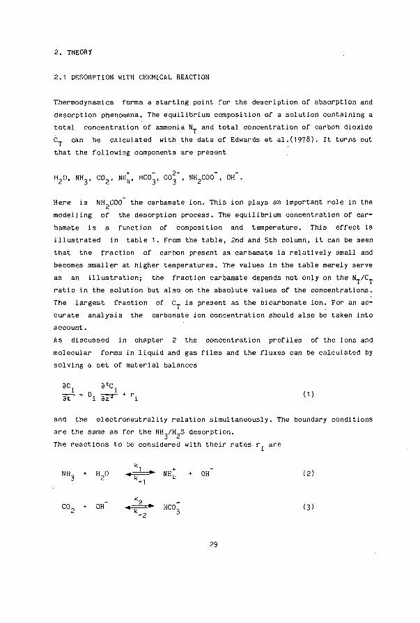
Thermodynamics forms a starting point for the description of absorption and desorption phenomena. The equilibrium composition of a solution containing a total concentration of ammonia N_ and total concentration of carbon dioxide C can be calculated with the data of Edwards et al.(1978). It turns out that the following components are present

H20, NH-, CO-, NH*, HCO" C0^~, NH2COo", 0H~.

Here is NH-COO the carbamate ion. This ion plays an important role in the modelling of the desorption process. The equilibrium concentration of car­bamate is a function of composition and temperature. This effect is illustrated in table 1. From the table, 2nd and 5th column, it can be seen that the fraction of carbon present as carbamate is relatively small and becomes smaller at higher temperatures. The values in the table merely serve as an illustration; the fraction carbamate depends not only on the N_/C ratio in the solution but also on the absolute values of the concentrations. The largest fraction of C„ is present as the bicarbonate ion. For an ac­curate analysis the carbonate ion concentration should also be taken into account. As discussed in chapter 2 the concentration profiles of the ions and molecular forms in liquid and gas films and the fluxes can be calculated by solving a set of material balances

3C. 32C. 3T'W-i (,)

and the eleetroneutrality relation simultaneously. The boundary conditions are the same as for the NH-,/HpS desorption. The reactions to be considered with their rates r. are

l

OH (2) NH

co2

+

+

H20

OH"

- ' ►

'"- ,

-V K

HCO" (3)

29

k3 2-HCO + OH -<-.kJ » CO^ + H20 (4)

C0 2 + 2 NH « k » NH2C00 + NH^ (5)

There is also a reaction of CO? with water to bicarbonate (Savage et al. (1980)). At higher pH values this mechanism is of little importance. Reaction 2 is instantaneous; this was simulated using very high values of the rate constants. The rate constants of reaction 3 were measured and correlated as a function of temperature by Pinsent et al.(1956a). Savage et al.(1980) have shown that Pinsent's formula, valid to 40 °C, can be used up to 100 °C. According to Astarita et al. (1981) reaction 4 is instantaneous. Reaction 5 is discussed by Danckwerts (1975) and Danckwerts and Sharma (1966). The forward reaction can be expressed as

rH = k1)[C02][NH33 (6)

and the backward reaction

[NH2C00 ][NH1J] r-4 = % K4 [NHJ (?)

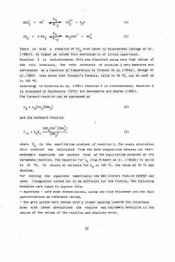
where Kü is the equilibrium constant of reaction 5. For every simulation this constant was calculated from the bulk composition because our ther-modynamic equations use another form of the equilibrium constant of the carbamate reaction. The equation for k from Pinsent et al. (1956b) is valid to 40 °C. To obtain an estimate for k. at 100 °C, the value at 40 °C was doubled. For solving the equations numerically the NAG library routine D03PGF was used. Integration turned out to be difficult for the routine. The following measures were taken to improve this: - equations 1 were made dimensionless, using the film thickness and the bulk concentrations as reference values. - the grid points were chosen with a closer spacing towards the interface. Even with these precautions the routine was extremely sensitive to the choice of the values of the relative and absolute error.

30

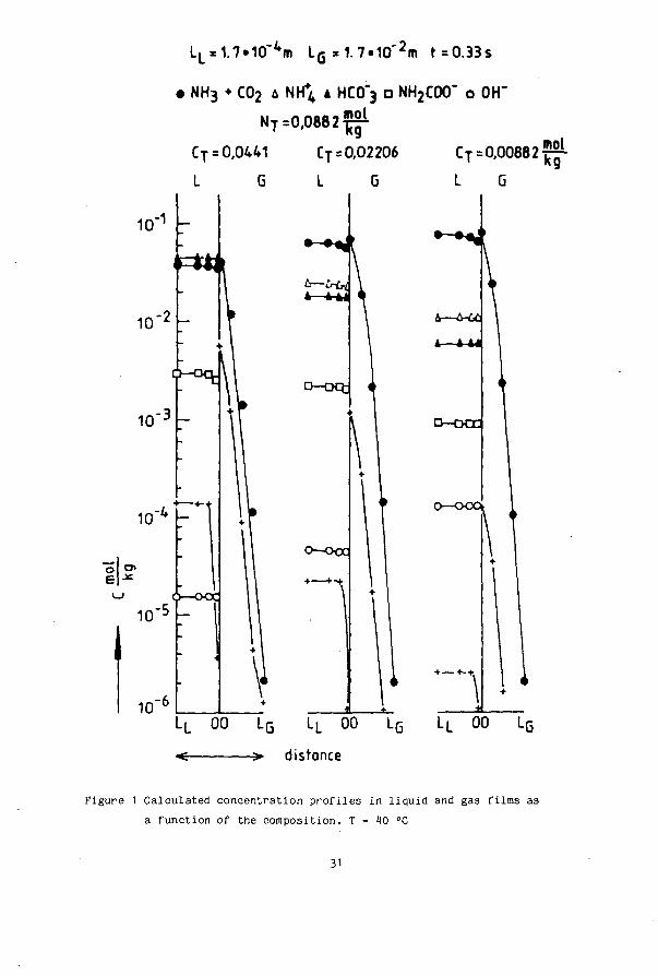
LL = 1.7»10'4m LG=1.7»10"2m t=0.33s

• NH3 ♦ CO2 A NH4 4 HCO"3 D NH2C0O" O OH"

NT =0,0882 ^

CT = 0,0441 CT = 0,02206 CT = 0 , 0 0 8 8 2 ^

L 6 L G L O

L—u-6^

D - D Q ;

O—OCC

.L 00 LG LL 00 LG

< > distance

&—6-6£

A — l - U

D—DCE

k

Figure 1 Calculated concentration profiles in liquid and gas films as a function of the composition. T = W °C

31

3. RESULTS

3.1. COMPUTER SIMULATIONS

The simulations were performed for a constant total ammonia concentration in the bulk of the liquid of N = 0.0882 mol-kg" . The total carbon dioxide

-1 -1 concentration C was varied from 0.01141 mol-kg to 0.00882 mol-kg . , giving molar concentration ratio's R = N_/C from 2 to 10. Figure 1 gives the concentrations as a function of the position in the film, at a contact time of 0.33 s, for R values of 2, 4 and 10. The horizontal scale in the gas (L_) is 100 times larger than that of the liquid (L ). In figure 2 the total fluxes of NH and CO are given as a function of the composition. The con­tribution of the different ions in the total carbon flux as a function of the composition and temperature is given in table 1 . The following aspects can be remarked from the calculations.

- In table 1 the relative contributions of different species to the flux are given. This contribution has been calculated from the depletion of the species in the film. It can be seen that at HO °C the largest fraction of the total CO- flux is due to the carbamate ion, which represents only 6 -10 it of the total carbon. At 100 °C the carbamate fraction has become so small and the rate constant k_ so large that at this temperature the bicar­bonate ions give the largest contribution to the flux. In table 1 the two ionic contributions do not sum up to 100 %, the difference being the molecular C0_ flux. For two compositions in the table ( R = 6 and 10 at 100 °C) the sum of the ionic contributions is larger than 100?. In these situa­tions the C0_ profile has a maximum, which is not visible in figure 1 , due to accumulation of C0_ in the film. This effect gives a negative contribu­tion of the molecular form to the total carbon flux. This profile shape is also reported by Cornelisse et al.(1980).

- Except for CO the concentration profiles in the liquid are relatively flat. For NH. this is caused by its high gas phase resistance. For HC0.. the cause is firstly the slow decomposition rate of reaction 3, and secondly,

2-but this is a «econd order effect, the production of HC0.. from CO, accord­ing to reaction 4. As a consequence of electroneutrality this also gives a flat profile of the NH^ ion.

32

,-3 -

n"5

N U =0.0882^-

10 12

Figure 2 Calculated fluxes of NH, and CO. as a function of the composition. T «■ 40 °C

Table 1 Fraction carbamate and contribution of the ions in the carbon flux as a function of the composition N„= 0.0882 mol'kg

HO °C 100 °C

% C as % C-flux % C-flux ( C as % C-flux % C-flux

2 4 6 10

NH2C00

6.9 9.8 10.5 10.1

NH2C00

93 96 95 9M

HCO +C03

1 0.9 0.9 0.8

NH COO

1.8 2.7 3.0 3-3

NH2C00

7 14 18 23

HC0,+C0

80 85 83 79

33

- Ammonia is at equilibrium in the liquid film with local concentrations of OH and NH.. For carbon dioxide considerable deviations from equilibrium occur. The difference from the equilibrium constants of the reactions 3 and 5 and those calculated from local concentrations may be as much as a factor five to ten. The deviations are the largest at the interface. Moreover, the concentration of C0? that would be in equilibrium with the participating reactants of reaction 3 is even different from that of reaction 5.

- The interfacial concentration of NH is almost constant. The interfacial concentration of CO however changes in time (figure 3). The influence on

the fluxes is not large. We observed an average difference of 5% in the overall fluxes compared to calculations with interfacial concentrations of the molecular forms constant in time, the latter method giving the highest values. The influence is small because the absolute concentration of C0? at the interface is small. With absorption however situations may occur where this interfacial concentration is higher and so the effect more pronounced. The numerical method used to solve the partial differential equations required considerable amount of computing time to integrate the equations with changing interfacial concentrations. The time dependancy of the interfacial concentra­

tions cannot be specified at forehand, but has to be determined by an iteration upon [NH_]. . and [CO.,]. , over a small time slice until the 3 int 2 int

0.2 0.3 0.4 - time (sec.)

Figure 3 Evolution of the norma­l ized in te r fac ia l concentrations

as a function of time.

mass balances of NH, and C0? over gas and l iquid are s a t i s f i e d . In overall the limiting case when the value of the time slice is chosen as the integra­tion (contact) time, the calculation has been done with constant interfacial concentrations. This means that for this last method the overall mass balance is satisfied for the whole contact time but not necessarily at intermediate times.

3

As the difference in the fluxes for both calculation methods is not that great, simulations were preferably done with constant interfacial con­centrations.

- It can be remarked that the flux of carbon dioxide is about a factor 30 lower than that of hydrogen sulphide under conditions of equal total molar composition. This despite the fact that carbon dioxide is the more volatile of these components. The flux of ammonia is only 20 % lower.

3.2. DEVELOPMENT OF A SIMPLE MODEL

Even with a large computer the numerical methods used above are too un-wieldly for design calculations for desorption columns. So simpler means of estimating the fluxes are required. The problem is formed by the parallel reactions 3 and 5 both yielding CO. and the coupled reaction 2. A good summary of the literature dealing with mass transfer and reaction in parallel can be found in the book of Westerterp et al. (1981). Unfortunately the examples given deal mainly with absorption with irreversible kinetics. The work of Pangarkar and Sharma ( W O . who studied the absorption of CO and NH , is mentioned here as an example. The problem of desorption with a parallel reaction was also encountered by Mahajani and Danckwerts (1983). They studied the rate of desorption of CO. from potash solutions with and without the addition of alkanolamines. Assuming that all concentrations except that of CO. remain constant in the film they used the enhancement factor equation of the fast regime with a Hatta number based upon the sum of the two forward reaction rate constants. This theory does not work in general because the underlying assumption of a constant CO concentration that would be in equilibrium with the reactants is violated. It is to be expected that the fluxes will be a function of the bulk and interfacial concentrations of the participating reactants and the forward and backward rate constants. As one might imagine the authors were not able to derive analytical expres­sions for the fluxes. Our approximate theory will assume pseudo first order kinetics. This is justified by the concentration profiles given before, but will also take into account the reversibility of the chemical reactions. The reactions 3 and 5 involving CO can be written in a pseudo first order form as

35

HCO

k 2 / / k - 2 [HCO ] , [NH2C00 ]

C ° 2 K2 = [C02] S [C02]

.\\ . - cK]

k A \ k - K [OH ] - K 4 V £NH„]2 3J

NH2COO

Before continuing with the parallel CO„ reactions, let us first have a look

at a single reversible chemical reaction of finite speed.

Such reaction can be represented as

f f ["3*1 A ■« , ► B , B is non volatile. K = -— = -FT4 at equilibrium, gas k

b • b ^ ]

The enhancement factor for this reaction, flux divided by the product of driving force and (physical) mass transfer coefficient, can be found in Danckwerts (1975). According to the Danckwerts surface renewal model the following expression for the enhancement factor holds

E = (K+1)/(1+Ha2(1+K)/K) (g) K + /(1+Ha2(1+K)/K)

with the Hatta number

/(D k ) Ha = ~ - (10)

kl

This relation covers the three regimes (figure 4) (i) E -► 1 when K -» 0 , the equation for a physical absorption or

desorption

(ii) E ■» /(1 + Ha ) when K >> Ha, the well known equation for the fast reaction regime

(iii) E -► 1 + K when Ha >> K, the equation for the instantaneous regime

36

Figure H Enhancement factor as a function of the Ha number.

K=100

HQ t - 1

Figure 5 Relative difference between enhancement factors of surface renewal and film theory as a function of the Ha number.

37

Other equations for the enhancement factor can be found in literature. They depend on the hydrodynamic model chosen and the boundary conditions of the governing differential equations. The use of the surface renewal equation is a conscious choice. The enhancement factor as predicted by the penetration theory is not convenient due to the appearance of error functions. An equa­tion for the enhancement factor proposed in the article of Shah and Sharma (1976) was found to be both less convenient and less accurate. The predic­tions of the equations of the film and surface renewal theory are, according to Danckwerts (1975), numerically almost the same. For the interval of Ha numbers we will encounter for this desorption problem (Ha » 1) a not unim­portant discrepancy exists between the surface renewal (SR) and film theory (FT). In figure 5 the relative difference in prediction between the two models has been plotted. We observe that around Ha equals one the film model can have an error of 5%. At low and high Hatta numbers the difference is small indeed. We give attention to this difference as we will need two enhancement factors, so the differences may accumulate. Now we consider desorption with two reactions in parallel. If both com­ponents 'B' are in excess it can be easily shown that in the fast reaction regime the total enhancement due to the two reactions follows

Dk Dk

kl kl

Here are k and k the two forward reaction rate constants of the paral­lel reactions. Equation 11 was used by Mahajani and Danckwerts (1983). At first glance an astonishing equation because the enhancement for desorption is independant of the magnitude of the backward reaction constants. These influence only the equilibrium value of [A]., and in this manner the driving force. The expression we have tested against our numerical results is a generalisa­tion of equation 11

Etot - ' < E? ♦ Eg " 1 ) (12)

where E and E_ are the individual enhancement factors of the two parallel reactions calculated with equation 9. The '-1' sets the enhancement factor to one if both reaction rate constants go to zero. Equation 12 is easily

38

seen to predict limiting cases such as physical desorption and those situa­tions where either of the two reactions has an overruling effect on the desorption rate. Let us return to the NH,-CO_ desorption. We assume that all components have the same mass transfer coefficients. For the parallel reactions we have two

i i Hatta numbers, Ha„„. and Ha.,„ __. with corresponding K_ and Kh values.

HLU3 Nn2LUU d 4 According to equation 9 these give two enhancement factors, E„„„ and E,,„ ™~- The Hatta number for the HCO, reaction, /(Dk„[OH ])/k. , has a value Nn2tyUU . i c 1 of about 0.60 at 40 °C and 4 at 100 °C. The pseudo first order K' -value for the HC03 reaction, [HC0-]/[C0o], is large compared to Ha „_ so that equa-

i *- p nl^U3

t ion 9 behaves such that E„_. = / (1 + Hau.„ ) . HLUj nUU3

For the NH.C00 reaction the quantity /(Dkü[NH.])/k. has a value of 4 at 40 °C which changes to 6 at 100 °C. The pseudo first order K. -value for this reaction, [NH COO ]/[C0_], is a strong function of the composition. For the compositions studied its value is in the range of 1 to 300 at 40 °C ,

I

and between 0.03 and 1.5 at 100 °C. At 100 °C where K„ < Ha.,„ nnn the 4 Nn2CUU

enhancement of the carbamate reaction is small because of the small amount of carbamate in the solution. So here we observe a shift in behaviour of the

2 f

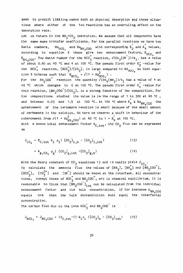
enhancement from /(1 + Ha„„ . m ) at 40 °C to 1 + K„ at 100 °C. With a known total enhancement factor E f the C0o flux can be expressed

JC0 2 " EC,tot kl "l( ^ A . b " ^ l . l n t ' ( 1 3 )

g.C02 g 2 g.int 2 g,b

With the Henry constant of C0_ equations 13 and 14 easily yield J . * + ^ u2 _

To calculate the ammonia flux the values of [NH ], [NH.] and [NH C00 ], - 2- -

[HCO,], [CO, ] and [OH ] should be known at the interface. All concentra­tions, except those of HCO, and NH-C00 , are in chemical equilibrium. It is reasonable to think that [NH?C00 ]. can be calculated from its individual enhancement factor and its bulk concentration. If for instance E M U

Nn2OUU

equals one then the bulk concentration must equal the in te r fac la l concentration. The carbon flux due t o the ions HCO- and NH-C00 i s

JHC03 + JNH2C00 " ^ C . t o t f " V l ( [ C °2 ] b " ^ V i n t ' ( 1 5 )

39

From equation 12 it can be seen that from the enhancement (E„ . ,.-1) in equation 15, a fraction (E,,„ „__-1) /(E„ . .-1) is due to the enhancement

Nn2LUU L , t O t by the NH.COO react ion. This gives for J„„ „ „ d NH2UUO

2

JNH2C00 " ( ^ ; ^ 1 ) } ' l P1 ( C C°2 ]b " ^ I n t '

fF - I I 2 vr,NHgCOO .

= ( E C , t o t - 1 ) EC,tot C0> (

As we know that

JNH2C00 ■ k l p l <CH2COO"3b " CN H2C 0 0"]int ) ( 1 7 )

i t follows from equation 16 and 17 that

[NH2C00-] int - [NH2C00-]b - J&&±- 08)

The value of [HCO ] . can be calculated most accurately from the to t a l carbon flux

JC02 " k l p l ( CT.tf CT,int> C19)

with

CT = [C02D + [HC0~] + [CO2"] + [NH2C00_] (20)

It follows from equation 19 and 20 that

[HC0-].nt ♦ [ C o f ] . ^ - CTfb - ^ _ [c02].nt_ [NH2COO-]lnt

(21) 2- - -

As CO, i s in equilibrium with HCO- and OH , the equilibrium constant of

reaction 4 can be used to eliminate th i s concentration. This gives

JC0

C H C ° 3 ] - - ~ l » W » - ] l n t ^^ 40

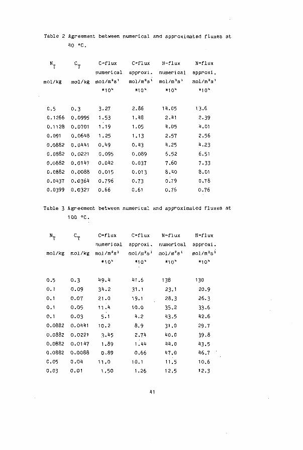
Table 2 Agreement between numerical and approximated fluxes at 1)0 °C.

NT

mol/kg

CT C-flux C-flux N-f lux N-flux

numer ica l a p p r o x i . numer ica l a p p r o x i .

mol /kg mol /m 2 s ' m o l / m ' s ' mo l /m 2 s ' mol /m 2 s '

«101* *10" «lO1* *10"

0.5

0 .1266

0.1128

0.091

0 .0882

0.0882

0.0882

0 .0882

0.01)37

0.0399

0 . 3

0 .0995

0 .0701

0 .0618

o.ow 0.0221

0.011)7

0 . 0 0 8 8

0.0361)

0 .0327

3-27

1.53

1.19

1.25

0 .H9

0 .095

0 .012

0 . 0 1 5

0 .796

0 . 6 6

2.86

1.18

1.05

1.13

0 .13

0 .089

0.037

0 .013

0.73

0.61

11.05

2.1)1

1.05

2.57

11.25

6 .52

7.60

8.M0

0.79

0.76

13.6

2 .39

D.01

2.56

1.23

6.51

7.33

8 .01

0 .78

0 .76

Table 3 Agreement between numerica l and approximated f l uxes a t

100 °C.

C-f lux C-f lux N-f lux N-flux numerica l a p p r o x i . numer ica l a p p r o x i .

m o l / k g

0 .5

0 .1

0 .1

0 .1

0.1

0.0882

0.0882

0.0882

0 .0882

0 .05

0 .03

m o l / k g

0 . 3

0 . 0 9

0 . 0 7

0 . 0 5

0 . 0 3

0.01)1)1

0 .0221

0 .0117

0 . 0 0 8 8

0.O4

0 . 0 1

m o l / m a s '

* 1 0 *

1)9.1

3 1 . 2

2 1 . 0

1 1 . 1

5 .1

1 0 . 2

3 .15

1 .89

0 . 8 9

11 . 0

1.50

m o l / m 2 s '

«lo­

l l . 6

31.1

19.1

10 .0

1.2

8 .9

2 .71

1.11

0 .66

10 .1

1.26

m o l / m 2 s '

«10"

138

23.1

2 8 . 3

3 5 . 2

13 .5

31 .0

10 .0

11 .0

1 7 . 0

11 .5

12 .5

mo l /m 2 s

«10"

130

20.9

2 6 . 3

33 .6

12 .6

29 .7

39 .8

13 .5

16 .7

10 .6

12.3

11

so that tHC03]int i s a f u n c t i o n o f [°H 1< t> this in turn is a function of J„„ as ammonia determines the pOH of the solution at the interface. NH3 For the flux J.,„ we write

JNH3 ■ kl Pl ( NT,b " "T.int5 ( 2 3 )

* k8 P8 ( CNH3]g,int " W (")

NT = [NH ] + [NH*] + [NH2C00_] (21)

_ t i n t int . „ .

V - mq?-t (25)

[co^D. . K _ 3 mt , , . KHC03 ' [HC03].nt[OH].nt

[ K ] i n t " CHC03]int + [NH2C00"]int + 2-[C°3~]int + [0H"]int (27)

3 giint , -. m™>= W T ^ (28)

The contribution of NH COO in the NH flux is taken into account with equation 23 (for the interface) and equation 27. We solved equations 22 to 28 with an iteration on [OH ]. . The equations can be written in sequence where a start value of [OH ] yields a new value for [OH ]. , which can be used again in the iteration. Starting with the value of the bulk concentration of OH , convergence was obtained after 5 recalculations of the equations. The results of a series of calculations done at different compositions are compared with the fluxes determined by the numerical method in table 2 for fO °C and in table 3 for 100 °C. The approximate fluxes are always slightly lower. For carbon dioxide deviations from 12$ at 10 °C to 25$ at 100 °C may occur. For ammonia the difference is usually smaller than 10$. A comparison between the approximate and numerical method for the individual component fluxes (such as J„„- ) is not given. We noticed that a smaller

HC03 approximated flux of e.g. HCO, is usually compensated by a larger ap­proximated flux of NH COO".

42

i 0.2 -

= 0.1

-

•

o

•

o

• 0 :

• •

° 0

computed

•

o

I

i 7

r NH3

r- " 2

i i 5000 10000

time (sec.) 15000 20000

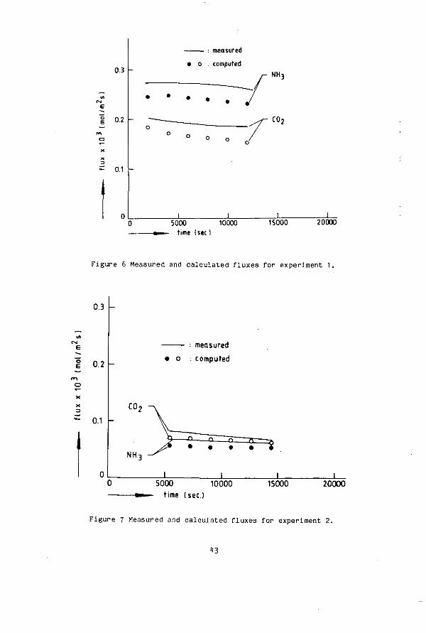
Figure 6 Measured and calculated fluxes for experiment 1,

0.3

CM

E

0.2

0.1 CO;

NH:

measured o : computed

I J_ _L 5000 10000

time (sec.)

J_ 15000 20000

Figure 7 Measured and calculated fluxes for experiment 2.

3

3.3. EXPERIMENTS

Under similar experimental conditions as described in chapter 2, three desorption experiments at 40 °C are reported here. The initial concentra­tions of the components were :

Experiment 1 N = 0.1399 mol-kg Experiment 2 N = 0.0101 mol-kg".

-1 Experiment 3 N = 0.1310 mol-kg .

1 C = 0.1172 mol-kg"1

C = 0.0352 mol-kg-1

CT = 0.1310 mol-kg"1

The results of the measurements are given in figure 6, 7, and 8, as the continuous lines and are compared with the values of the fluxes determined by the approximate method. The third experiment was done in a 0.18 M NaCl solution. This experiment provides a severe test of the thermodynamic framework used. The activity coefficients of the components are influenced by the high ionic strength. The C0? flux is very sensitive to the value of these coefficients. To show the influence we have calculated the fluxes for experiment 3 with the liquid assumed to be ideal. At a given composition N„,C_ the fluxes are then higher because the position of the equilibria of the C0_ reactions is shifted towards that of the molecular form. In an experiment the total concentrations become lower and so do the fluxes (figure 6 and 7). This does not hold for ammonia in experiment 3 (figure 8). In this experiment JMU increases in time. As a result of the high initial Nn 3 carbon concentration J„n has a high value. This results in a liberation of

+ t'U2

NH. from NH,., at a rate which is higher then the flux of ammonia to the gas. So the net effect is a decreasing N_, with an increasing [NH ], which is favourable for a higher ammonia flux. The agreement between calculated and predicted fluxes is seen to be good.

44

0.6 -

0.5 -

0.4

0.3 -

0.2

- 0.1 -

-

-

-

A

0

A

•

A

O

1

•

1

&

cV'

A

•

A

\° A

•

• , 0 i , £

A

O

\ ^ A

• - P 5

1

mpncurpri I I I C U J U I C U

computed non ideal liquid computed ideal liquid

^ c o 2

>NH3

l 1 5000 10000 time (sec.)

15000 20000

Figure 8 Measured and calculated fluxes for experiment 3. [NaCl] = 0.18 M.

15

1. CONCLUSION

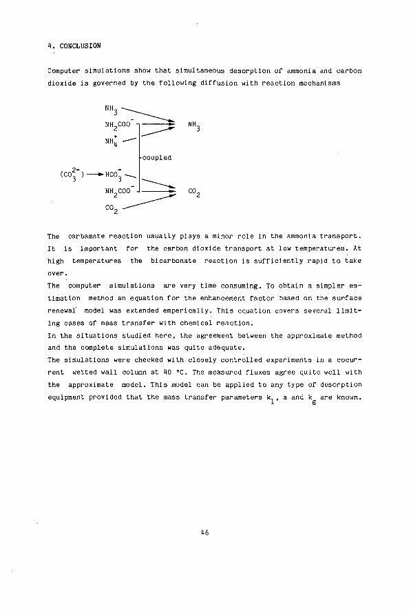
Computer simulations show that simultaneous desorption of ammonia and carbon dioxide is governed by the following diffusion with reaction mechanisms

(co^-) -HCO,

NH„

coupled

C0„

The carbamate reaction usually plays a minor role in the ammonia transport. It is important for the carbon dioxide transport at low temperatures. At high temperatures the bicarbonate reaction is sufficiently rapid to take over. The computer simulations are very time consuming. To obtain a simpler es­timation method an equation for the enhancement factor based on the surface renewal' model was extended emperically. This equation covers several limit­ing cases of mass transfer with chemical reaction. In the situations studied here, the agreement between the approximate method and the complete simulations was quite adequate. The simulations were checked with closely controlled experiments in a cocur-rent wetted wall column at 40 °C. The measured fluxes agree quite well with the approximate model. This model can be applied to any type of desorption equipment provided that the mass transfer parameters k , a and k are known.

46

SYMBOLS

C concentration C total CO concentration E enhancement factor Ha Hatta number J flux K equilibrium constant

i

K pseudo first order equilibrium constant k. mass transfer coefficient k. reaction rate constant

m partition coefficient (mol-kg )liquid

N total NH concentration mol-kg R concentration ratio NT/C (-)

-1 -1 r, production rate mol-m »s T temperature °C t time s z coordinate m

Greek

subscript

b

C

f

g i

i n t

1

t o t

bulk or backward C02

forward gas

component i in terface l iqu id t o t a l

m o l '

mol •

(-) (-) mol ■

m o l '

(-) m-s

, -1 ■kg . , - 1 ■kg .

- 2 - 1 >m »s

• k g " 1

■1

m -mol . - 1

3

(mol - • kg

- 1 •s . or

)gas

-3 density kg-m

17

6. LITERATURE

Astarita G., Savage D.W., Longo J.M., 1981, Promotion Of CO Mass Transfer In Carbonate Solutions, Chem.Eng.Sci., 36, 581-588.

Cornelisse R., Beenackers A.A.CM., Beckum van F.P.H., Swaaij van W.P.M., 1980, Numerical Calculation Of Simultaneous Mass Transfer Of Two Gases Accompanied By Complex Reversible Reactions, Chem.Eng.Sci., 35, 1215-1260. Danckwerts P.V.,1975,Gas Liquid Reactions,Mc-Graw Hill,New York. Edwards T.J., Maurer G., Newman J., Prausnitz J.M., 1978, Vapor—Liquid Equilibria In Multicomponent Aqueous Solutions Of Volatile Weak Electrolytes, AIChE J., 24, 966-976. Hoogendoorn G.C., Wesselingh J.A., Castel S.D.L., Theory And Experiments On The Simultaneous Desorption Of Volatile Electrolytes In A Wetted Wall Column, part 1 Ammonia And Hydrogen Sulphide Desorption, submitted for publication to Chem.Eng.Sci.. Mahajani V.V., Danckwerts P.V., 1983, The Stripping Of CO. From Amine Promoted Potash Solutions At 100 °C, Chem.Eng.Sci., 38, 321-327. Pangarkar V.G., Sharma M.M., 1974, Simultaneous Absorption And Reaction Of Two Gases: Absorption Of C0„ And NH, In Water And Aqueous Solutions Of Alkanolamines, Chem.Eng.Sci., 29, 2297-2306. Pinsent B.R.W..Pearson L.,Roughton F.J.W., 1956a, The Kinetics Of Combination Of Carbon Dioxide With Hydroxide Ions, Trans. Faraday Soc, 52, 1512-1520. Pinsent B.R.W., Pearson L., Roughton F.J.W., 1956b, The Kinetics Of Combination Of Carbon Dioxide With Ammonia, Trans. Faraday Soc, 52, 1594-1598.

Savage D.W., Astarita G., Joshi S., 1980, Chemical Absorption And Desorption Of Carbon Dioxide From Hot Carbonate Solutions., Chem.Eng.Sci., 35, 1513-1522.

Shah Y.T., Sharma M.M., 1976, Desorption With Or Without Chemical Reaction, Trans.Instn.Chem.Engrs., 54, 1-41.

Westerterp K.R., Swaaij van W.P.M., Beenackers A.A.CM., 1984, Chemical Reactor Design And Operation, John Wiley, 495-570.

48

CHAPTER 1)

THEORY AND EXPERIMENTS ON THE SIMULTANEOUS DESORPTION OF VOLATILE ELECTROLYTES IN A WETTED WALL COLUMN

- AMMONIA, HYDROGEN SULPHIDE AND CARBON DIOXIDE DESORPTION -

G.C. Hoogendoorn, CM. Sidawy, J.A. Wesselingh Delft University of Technology Department of Chemical Engineering Julianalaan 136 2628 BL Delft Netherlands

ABSTRACT

Experiments are presented of the simultaneous desorption of NH,, H S and CO from water at a stagnant water gas interface. The experiments can be des-cibed with a model that can be seen as the the union of the two models presented in the chapter 2 and 3 describing the NH - H S and NH - CO desorption respectively.

1. INTRODUCTION

This is an extension of previous work to the simultaneous desorption of three components from water undergoing chemical reactions. In practice stripping operations usually have at most two major strippable components (or are regarded to have only two components): -sour water in oil refineries primarily contains ammonia and hydrogen sulphide -process water in the production of urea fertilizer mainly contains ammonia and carbon dioxide. Nevertheless cases with more components do occur and we thought it worthwile to pay some attention to the subject.

19

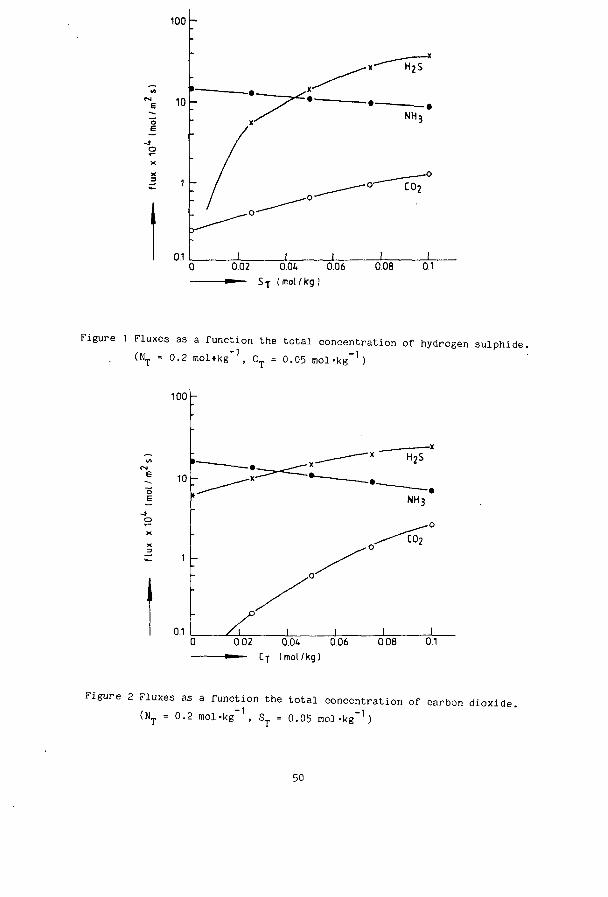
0.02 O.Ot 0.06 0.08 0.1 ^ — S-j- ( mol/kg !

Figure 1 Fluxes as a function the total concentration of hydrogen sulphide. (NT - 0.2 mol+kg"1, CT = 0.05 mol-kg"1)

100

0 0.02 0.0*. 006 ■' Cf (mol/kg)

008 0.1

Figure 2 Fluxes as a function the total concentration of carbon dioxide (NT = 0.2 mol-kg" , ST = 0.05 mol-kg~1)

50

2. RESULTS

2.1. DESORPTION WITH CHEMICAL REACTION

As we have shown earlier the mass transfer of the volatile electrolytes studied can be described by a series of coupled partial differential equations. These can in principle be solved by numerical integration using the appropriate initial and boundary conditions. We have not attempted to do this for three components. Already with the system NH -CO, considerable difficulties were encountered. It is to be expected that these will be much worse if three extra equations ( for [H SL , [H S] and [HS ] ) are added. The calculation scheme for the NH,-C0? desorption was directly extended to one for NH , H.S and CO.. The only change to the NH- - CO- calculation scheme is an addition of the equations giving the H.S flux. This modification can be done by inserting the equations for J (equations

n zo 23 - 25 from part 1 ) in a suitable place in the calculation scheme of amonia and carbon dioxide ( between equation 24 and 25 in part 2 ). Furthermore the electroneutrality relation at the interface has to be modified to include the new species. The behaviour of the desorption can be illustrated with some calculations. These have been done for a wetted wall column with cocurrent gas and liquid flow. Values of parameters have been taken at 40 °C. Figure 1 gives the fluxes of NH , H-S and CO- as a function of the total -1 sulfur composition ( N = 0.2 and C = 0.05 mol-kg ). Figure 2 is shows the same but for different total carbon concentrations ( N_ = 0.2 and S_ »

-1 0.05 mol-kg ), and in figure 3 the total nitrogen is changed at constant acid load ( ST = 0.05 and C = 0.025 mol-kg"1 ). From figure 1 and 2 can be seen that an increase in concentration in one of the acid components causes an increase in the flux of the other acid gas and a decrease of that of the basic gas ammonia. Also the reverse is true: increasing the concentration of ammonia makes the fluxes of H S and C0_ lower ( figure 3 ). The results shown in the figures include two effects. The most important one is the shift in the equilibria and therefore in the driving forces. Secondly the enhancement factors of the components, and so the overal mass transfer coefficients, also change with the composition. If more acid gas (e.g. S in figure 1) is added to a mixture of constant N and C_ then:

51

100

10

0.1

0.01 0.1 I

0 2 0.3 - NT (mol /kg)

0.4

H,S

0.5

Figure 3 Fluxes as a function the to ta l concentration of ammonia. (ST = 0.05 mol-kg"1, CT = 0.025 mol-kg"1)

decreases because H S reacts with ammonia to form NH.HS and so [NH,] i s lowered increases because the pH is s l i gh t ly lowered by the S_ and so [CO,]. is raised

, increases because of the increasing amount of S_ the [H„S], i s increased

explanation of figures 2 and 3 i s s imi lar .

52

2.2 EXPERIMENTS

The wetted wall column is the same as described in chapter 2. Our only new experience was that the difficulty of the experiments increases strongly with the number components studied. Especially when the components react with each other, any error in the determination in the concentration in one of the components also propagates in the equilibrium composition of the mixture as a whole.

Three succesful experiments can be reported with initial concentrations:

Experiment 1 N = 0.213 mol-kg" S = 0.016 mol-kg" C = 0.113 mol-kg"1 -1 -1 -1

Experiment 2 N = 0.160 mol-kg S = 0.060 mol-kg . C = 0.088 mol«kg . -1 -1 -1

Experiment 3 N = 0.167 mol-kg S = 0.095 mol-kg C = 0.085 mol'kg The fluxes are given as a function of time in figures 1, 5 and 6. The agree­ment between experimental and calculated fluxes is reasonable. Differences are not only due to experimental errors and inaccuracies in the calculations but also to uncertaincies in the thermodynamic data. We have observed that (especially for Ju „) the fluxes are overestimated if the liquid is assumed ri 2 o to be ideal but are slightly underestimated if non ideality is incorporated.

53

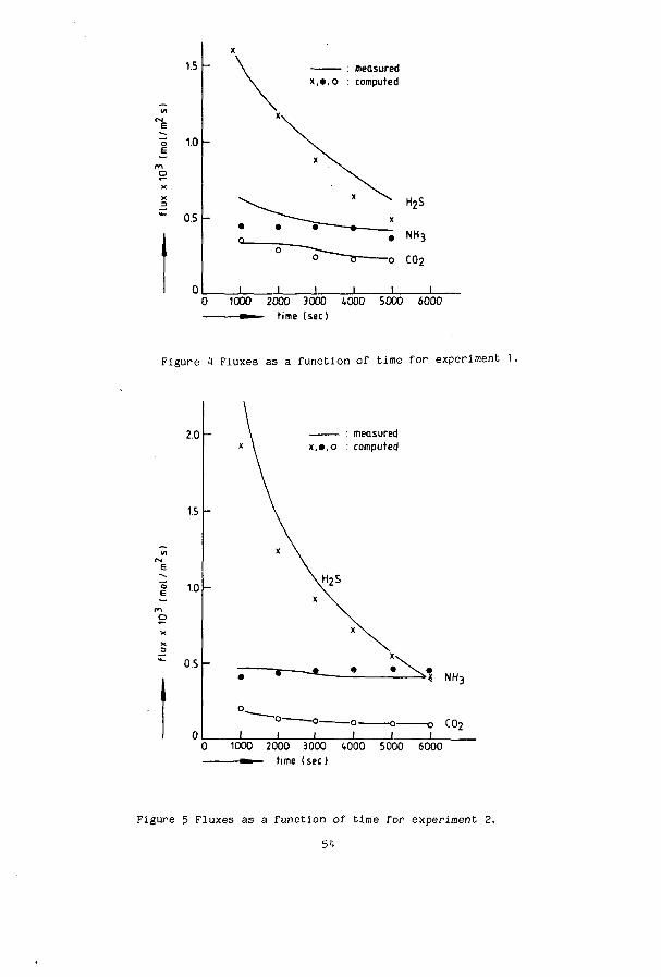
B

"o E

rry O

1.5

1.0 "

0.5

measured x,»,o : computed

1000 2000 3000 i.000 5000 6000 — ■ time (sec)

Figure 4 Fluxes as a function of time for experiment 1

2.0

1.5

1.0

05 -

measured x,»,o : computed

•% NH3

C02

1000 2000 3000 (.000 5000 6000 — ■ time (sec)

Figure 5 Fluxes as a function of time for experiment 2.

5i)

2.0

1.5

1.0

0.5

measured x,»,o : computed

NHq

"b C02 0 1000 2000 3000 (.000 5000 6000

^ — time (sec)

Figure 6 Fluxes as a function of time for experiment 3.

3. CONCLUSION

The simultaneous desorption of NH 3' H_S and C0? can be described with a model combining the NH - H S and NH,- CO? simulations. The model equations include equilibria for NH./NH* and H S/HS" with 0H~ everywhere in the liquid film and a column show good agreement with the model calculations.

kinetic expression for CO . Fluxes measured on a wetted wall

55

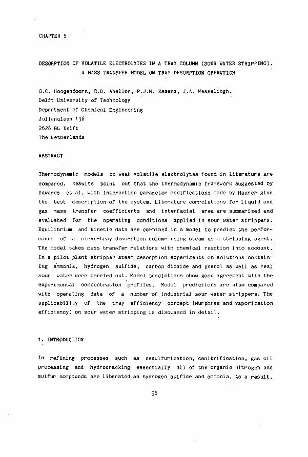
CHAPTER 5

DESORPTION OF VOLATILE ELECTROLYTES IN A TRAY COLUMN (SOUR WATER STRIPPING). A MASS TRANSFER MODEL ON TRAY DESORPTION OPERATION

G.C. Hoogendoorn, R.D. Abellon, P.J.M. Essens, J.A. Wesselingh. Delft University of Technology Department of Chemical Engineering Julianalaan 136 2628 BL Delft The Netherlands

ABSTRACT

Thermodynamie models on weak volatile electrolytes found in literature are compared. Results point out that the thermodynamie framework suggested by Edwards et al. with interaction parameter modifications made by Maurer give the best description of the system. Literature correlations for liquid and gas mass transfer coefficients and interfacial area are summarized and evaluated for the operating conditions applied in sour water strippers. Equilibrium and kinetic data are combined in a model to predict the perfor­mance of a sieve-tray desorption column using steam as a stripping agent. The model takes mass transfer relations with chemical reaction into account. In a pilot plant stripper steam desorption experiments on solutions contain­ing ammonia, hydrogen sulfide, carbon dioxide and phenol as well as real sour water were carried out. Model predictions show good agreement with the experimental concentration profiles. Model predictions are also compared with operating data of a number of industrial sour water strippers. The applicability of the tray efficiency concept (Murphree and vaporization efficiency) on sour water stripping is discussed in detail.

1. INTRODUCTION

In refining processes such as desulfurization, denitrification, gas oil processing and hydrocracking essentially all of the organic nitrogen and sulfur compounds are liberated as hydrogen sulfide and ammonia. As a result,

56

significant amounts of the latter components are found in refinery waste waters. A wide range of other contaminants will be present, including carbon dioxide, phenolics and various hydrocarbons. Such wastewater is generally known as "sour water" although it is slightly basic. The name "sour water" was probably coined due to the presence of the obnoxious H?S. Steam strip­ping, in packed or tray columns, followed by sulphur recovery or incineration is perhaps the most widely used process to eliminate these potential atmospheric pollutants. Tray columns installed show a large varia­tion in design. The number of trays installed may range from from 5 to 20, the amount of stripping steam from H to 20 J wt on feed. Part of this variability may be explained by the difficulty of predicting column performance. Ammonia, hydrogen sulfide, carbon dioxide and phenol in water are present in molecular and ionic forms; up to 14 relevant components can be recognized in the liquid. For some components (e.g. H_S) the main fraction is in a non strippable -ionic- form. Description of the stripping process therefore requires the application of the theory of mass transfer with chemical reaction. This paper intends to discuss all important aspects on tray desorption. These aspects can be classified as 1 . the evaluation of the vapour-liquid equilibria 2. the mass transfer coefficients and interfacial area for sieve trays 3. the development of a stripping model and testing this with experimental

data from laboratory tests as well as industrial-scale strippers H. a discussion of the concept of tray efficiencies.

2. BASIC DATA

2 . 1 . VAPOUR-LIQUID EQUILIBRIA

An equilibrium model i s used to determine how a cer ta in component dis­t r i bu t e s i t s e l f between the vapour and the l iquid phase. In the l iquid phase chemical react ions between the components occur. The following react ions are of in te res t for th i s study.

R . 1

R.2

NH + H 20 «, »• NH^ + OH"

H2S + H 2 0 ^ » HS" + H O *

57

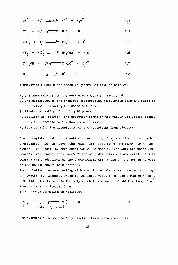
HS" + H20 « > S2~ + HO* R.3

C02 + H20 ^ » HCO~ + H+ R.4

HCO" + HgO « , - CO2" + HO* R.5

NH + HCO~ ^ ► NH2C00" + H20 R.6

C,HcOH + Ho0 < » C,Hco" + H.O+ R.7 b 5 2 6 5 3

H20 ,, » H+ + OH" R.8

Thermodynamic models are based in general on five principles:

1. The mass balance for the weak electrolyte in the liquid. 2. The definition of the chemical dissociation equilibrium constant based on

activities (including the water activity). 3. Electroneutrality of the liquid phase. 14. Equilibrium between the molecular forms in the vapour and liquid phase.

This is expressed by the Henry coefficient. 5. Equations for the description of the deviations from ideality.

The complete set of equations describing the equilibria is rather complicated. So to give the reader some feeling of the behaviour of this system, we start by developing two crude models. Here only the major com­ponents are taken into account and non idealities are neglected. We will compare the predictions of the crude models with those of the method we will select at the end of this section. The solutions we are dealing with are dilute. Also they invariably contain an excess of ammonia, which is the least volatile of the three gases NH , H?S and COp. Ammonia is the only volatile component of which a large frac­tion is in a non ionized form. If carbamate formation is neglected

NH3 + H20 « * NH4 + OH R.1 total N

For hydrogen sulphide the only reaction taken into account is

58

H2S H2O v : t o t a l S„

HS I

H30 R.2

In presence of the weak base NH, reaction 2 i s almost completely shifted to the right and therefore nearly the whole of the H?S is ionized; only a trace i s in the molecular form. The hydrogen and hydroxyl ions combine to form water. Because of e lec t roneu t ra l i ty the concentrations of the two major ions must be approximately equal : [HS ] « [NH^] » S

Then [NH ] = NT - [NH^] = NT - ST

and one expects a pa r t i a l pressure

V a ( N T V (1)

with the Henry coefficient of ammonia as the proportionality constant. This behaviour is indeed observed as can be seen in figure 1. The conditions shown there are typical of what might be found in the top of a sour water stripper.

a a.

x z a.

.02 .04 .06 .08 .10 .12 - ST mol.kg-1

Figure 1 Partial pressure of NH as a function of the total i -1

concentration of H S. T=100 °C, N = 0.15 mol-kg .

59

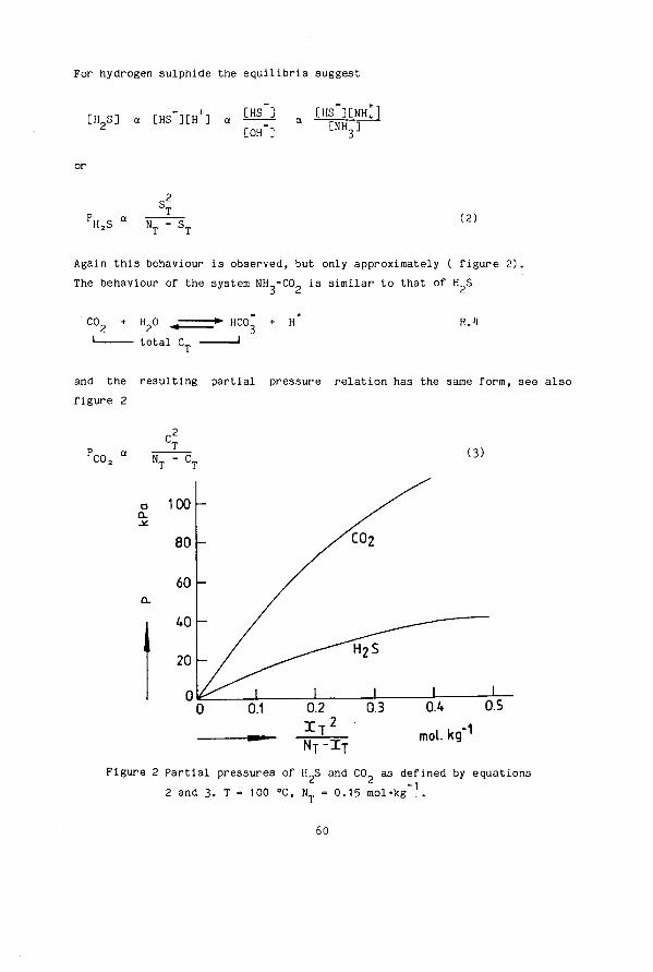
For hydrogen sulphide the equilibria suggest

CH.S] a CHS"][H+] a I M J a % ï ï ^ 2 [OH"] C N H3 ]

P a — rH 2S " NT - S T

(2)

Again this behaviour is observed, but only approximately ( figure 2). The behaviour of the system NH -CO. is similar to that of H S

C02 + H20 ^ 1 total C„

^ HCO + H I

R.H

and the resulting partial pressure relation has the same form, see also figure 2

P„„ a

N T - ^ T tnol. kg

Figure 2 Par t ia l pressures of H S and C0_ as defined by equations 2 and 3. T = 100 °C, NT = 0.15 mol-kg"1.

60

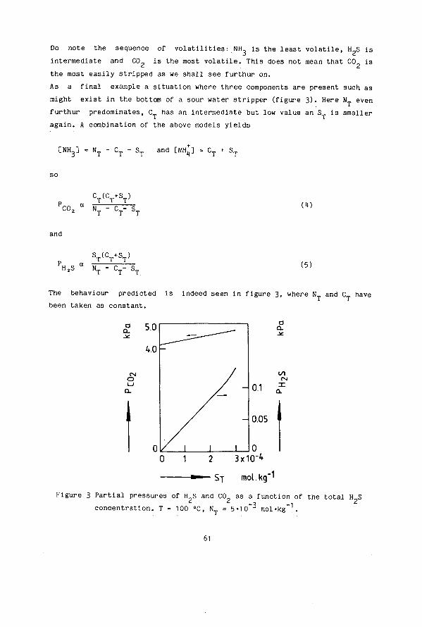
Do note the sequence of volatilities: NH is the least volatile, H2S is intermediate and C0_ is the most volatile. This does not mean that CO is the most easily stripped as we shall see furthur on. As a final example a situation where three components are present such as might exist in the bottom of a sour water stripper (figure 3). Here N even furthur predominates, C has an intermediate but low value an S is smaller again. A combination of the above models yields

[NH3] = NT - CT - ST and [NH,,] = C? + ST

C (C +S ) T T r

C02 " NT - CT- ST

(1)

and

H2S " NT - CT- ST (5)

The behaviour predicted is indeed seen in figure 3, where N_ and C_ have been taken as constant.

Q.

- 0.05

__ 0 2 3x10"^ - Sj mol.kg"^

Figure 3 Partial pressures of H2S and CO as a function of the total H S concentration. T = 100 °C, N = 5 -10~3 mol-kg"1.

61

The qualitative agreement of the above relations might make one believe that they are sufficiently accurate. This is not so however. The vapour liquid equilibria will be found to play a very important role in sour water strip­pers and more accurate relations are required. There are three major reasons for the inaccuracies: 1. The gases H S and C0„ are not completely dissociated as assumed above. 2. The effects of other reactions, especially those of carbamate and bicarbonate are not negligeable. 3. The solutions are non ideal. Even in the very dilute solutions of figure 3 the monovalent ions have activity coefficients of about 0.93-There are several models available in literature which do take these effects into account. - the model of van Krevelen, Hoftijzer and Huntjens (1919) - the model of Beutier and Renon (1978) - the model of Edwards et al. (1978) - the model developed by Wilson (1978) for the American Petroleum Institute

(API). The first three models have been recently discussed by Maurer (1980). Here we summarize his main conclusions. Because of the limited temperature (up to 60 °C) and concentration range (0.2 mol-kg . < N < 2.0 mol-kg ) in which the method of van Krevelen et al. can be used succesfully, this model is not applicable to sour water steam strippers, where very low concentrations (down to 10 ppm or less) are to be met at relatively high temperatures (usually 100 to 105 °C). From the work of Maurer, it is suggested that the model of Edwards et al. gives somewhat better results than the method of Beutier and Renon, espe­cially for the quaternary system NH,.- C0?- H-S - H.0. Based on more recent experimental work, Maurer has made some minor changes in the parameters of the model of Edwards et al. Maurer differs from Edwards with respect to the equilibrium constants Kuo and K nr,n, more and dif-* Ho" Nn2OUU ferent B and g values and a different formulae for calculating the 8. . interaction parameter, giving values 0.018 lower for Maurer. ion-ion F o o We have checked the Edwards, Maurer and Wilson models against available experimental data.

62

Table 1. Comparison of thermodynamio models . Wilson composi t ion d a t a have

been conver t ed t o moles /kg w a t e r .

T

°C mol-kg l i t

sou rce

P exp mm Hg

c a l c . l i t mm Hg

OWN CALCULATIONS i l

Edwards Maurer Wilson

da t a da t a da t a

mm Hg mm Hg mm Hg

100 NT 3.667 API 770.3 711.1 729.8 730.0 707.7

100

100

100

100

80

110

110

NT CT

NT

C T

NT CT

NT ST

NT sT

NT S T CT

NT ST CT

2.90

1 .15

3.71 1.11

5.11

0.153

6.51

1.9

5.11 1.11

2.383 1 .296

0.816

0.609

0.169

0.073

Edw/Mau

Edwards

API

Maurer

Edw/Mau

API

API

158.0

1211.1

133.1 319.3

923.0

13.0

1223.6

551.8

571

91.8

258.9 1616.8

5976.5

100.3 172.2

169.1

231.6/222

912.1/1180

110.9 316.1

921.1

19.9

1003.2

125.6

115.7/526

52.5/80.9

112.3

5170.7 7171 .6

90.5

155.5 176.2

210.8

991.3

111.1

330.1

918.0

26.1

868.8

151 .1

111.6

75.3

96.3 1137.2

1509.8

91 .2 158.8

187.1

219.7 1169.0

125.3 379.5

919.0

36.6

993.2

116.7

523.3 80.2

108.6

1372.0

5125.9

98.1

116.9 196.0

185.0

1688.5

383.5 395.1

919.3 19.8

836.9 602.2

110.5

102.5

112.3 551.8

7383.3

90.3 158.6

173.0

63

The method of Wilson is used exactly as described in his report. In the model of Edwards two simplifications are made: - Poynting corrections of the Henry constants are neglected; according to Maurer they can be neglected without causing a significant error if the total pressure is 10 MPa or less.

- Vapour phase fugacity coefficients are assumed to be unity; according to Beutier and Renon these coefficients do not differ more than ]% (2% for water) from unity if the total pressure is less than 0.2 MPa.

Some selected results of the comparison are given in table 1 . From table 1 it is clear that all reported results can not be reproduced exactly. The difference between our calculations and those reported by Edwards et al. are considerable. The computer program used for the calculations was developed by ourselves and checked as thoroughly as possible. For the parameters for which an iteration loop turned out to be neccesary, namely,

+ the ionic strength and the H concentration, the stop criteria were set at a -3 -5 sharp value: 10 % and 10 %, respectively.

It is remarkable that in general our calculations with the data set of Edwards et al. are closer to the experimental values than those reported by the group of Edwards. The calculations reported by Maurer can be reproduced. The small differences here between the calculated values have the same order of deviation as the fugacity coefficients from unity. We believe therefore that the reported calculated values by Edwards are erroneous. It was decided to use the method of Edwards with the revised parameters given by Maurer because these give, in general, slightly better results than the original parameters of Edwards. The Wilson method was not prefered because its thermodynamic framework is weaker than that of the others. Our vapour liquid equilibria were also extended to phenol. For this com­ponent, the equations for calculation of the equilibrium constant and the Henry constant are taken from Tsonopoulos et al. (1976) and Pawlikowski et al. (1983) respectively.

2.2. MASS TRANSFER COEFFICIENTS AND INTERFACIAL AREA (LITERATURE REVIEW)

The mass transfer parameters a, k and k ( and related subjects such as the tray efficiency and the number of transfer units ) of tray columns have been

64

the subject of a fair amount of investigation especially in the period from 1950 to 1972. These parameters are essential for designing columns for the physical separation of mixtures and also for chemical-physical operations such as oxidation, hydrogenation, chlorination and absorption or desorption with chemical reaction. Early research was dominated by the application and extension of the American Institute of Chemical Engineers research programme (1958). Most work in this period was done on bubble cap trays. In the period 1966 to 1972 research efforts diminished and shifted towards sieve trays. Appendix 1 gives a summary of literature correlations for the prediction of the mass transfer parameters in tray columns with sieve plates. Only two references (Nonhebel (1972) and Zuiderweg (1982) give equations for k , k and a. The correlations have been evaluated for the tray under study. Operating data, physical constants and tray details are given in table 2. The literature correlations show a surprisingly large spread in their predictions. This is illustrated in figure 1: for k the difference between minimum and maximum value is a factor of 65, for k this is a factor of 17.

g The data for the interfacial area are more consistent, the minimum and maximum differ by a factor of 1.1 . As the value of the parameters is essential for our desorption model, ex­periments have been carried out to determine them. The results of these experiments are given in figure H as 'This work'. The procedures used are briefly discussed below, more details are to be found in appendix 1. - k was determined in an air water simulator of the steam stripper. The Danckwerts chemical absorption (1975) method allows the determination of the interfacial area a and k . The value of k at 20 °C was corrected to 103 °C by assuming a square root dependancy of the mass transfer coefficient on the diffusivity. - a was determined in the steam stripper by absorbing CO- from steam in a NaOH solution. The interfacial area is obtained by fitting predicted con­centration profiles from a model containing a. as a parameter. - k was determined from experiments with desorption of NH from water. These experiments actually give the product of overall mass transfer coeffi­cient and interfacial area, from which with the known k and a , the k

I t g value can be calculated.

65

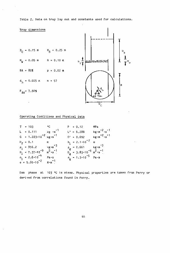
Table 2. Data on tray lay out and constants used for calculations.

Tray dimensions

Dc = 0.15 m Hg = 0.25 m

H^ - 0.05 m B = 0 . 1 0 m

BA = 80* p = 0.02 m

d. = 0.005 m n = 57 h

FBA= 7.92$

Operating Conditions and Physical Data

= 103 = 0.111

°c kg -1

G = 1 .223-10"2 kg-s"1 Hf = 0.1 m

- 956.2 = 7.37-10" = 2.8-10 5.05-10"2

-3 kg-m 2 -1 m -s Pa-s !• "1

N-m

P =0.12 MPa L' = 6.288 kg-m~2-s~1

-2 -1 G' = 0.692 kg-m -s hx =2.1 -10~2 m p = 0.661 kg-m s -5 2 - 1 D = 3.83-10 3 m -s n - 1.3-10~5 Pa-s

-3

Gas phase at 103 °C is steam. Physical properties are taken from Perry or derived from correlations found in Perry.

66

10 -2 — • Asano

E|i/>

- 10"3

10"

• P e r r y

— • Th i s work • Calderbank • Nonhebel

• Zuiderweg

_L 100 C

1.0 -

E|f>

- 10"

10" 100 C

E

< co E

• This work . .

• Zuiderweg • Perry • Nonhebel

10'

10'

• This work • Zuiderweg 2 t Zuiderweg 1

Nonhebel

100 C

Figure H Mass transfer coefficients and interfacial area at 100 °C. For Perry k, and k it is assumed a H2H m 1 g

67

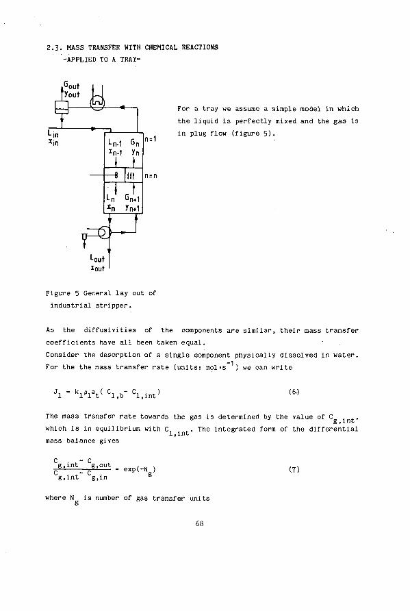
2 . 3 . MASS TRANSFER WITH CHEMICAL REACTIONS

-APPLIED TO A TRAÏ-

i6OUt fyout

■in 'in

< ^

Ln-1 Gn *n-1 yn

t , t III

J7 Ln Gn4l

n=1

n=n

? PS> □ T Lout lout

For a tray we assume a simple model in which the l iquid i s perfectly mixed and the gas is in plug flow (figure 5 ) .

Figure 5 General lay out of indus t r i a l s t r ipper .

As the di f fus ivi t ies of the components are s imi lar , the i r mass t ransfer coeff ic ients have a l l been taken equal. Consider the desorption of a s ingle component physically dissolved in water . For the the mass transfer r a t e (uni t s : mol-s ) we can write

J l " k l p l a t ( C l , b " ^ . i n t 5 (6.)

The mass transfer rate towards the gas is determined by the value of C . ,., g, int

which is in equilibrium with C, . ... The integrated form of the differential l . m t °

mass ba lance g ives C - C

g , i n t g .ou t C - C

g . i n t g , in

exp(-N ) g (7)

where N is number of gas transfer units

68

For a physical process it is common to eliminate the unknowns C, , . and 1 ,int

C . by introducing an overall transfer coefficient. For more difficult cases such as the absorption or desorption of two or more gases accompanied by chemical reactions this coupling of gas and liquid with overall coeffi­cients should be avoided. As shown by Cornelissen (1980) it can lead to strange results such as negative transfer coefficients. The effect of the chemical reactions is accounted for by an enhancement factor. The introduc­tion of overall transfer coefficients requires the knowledge of the enhancement factor for every volatile component. This is generally not known a priori. A descripition on the partial driving forces instead of overall bulk driving forces is to be preferred. Consider desorption with chemical reactions as defined by R.1 to R.8 . All reactions except R.5 and R.6 can be regarded as instantaneous as only proton transfer is involved. This means that for every reaction at every point in the liquid the equilibrium relation is obeyed. Reactions 5 and 6 have a finite rate. This implies that the chemical kinetics of the rate determining reactions

- OH C02 + OH « » HCO R.9

C02 + 2 NH „■ NH;i» NH2C00" + NH* R.10

play a role in the desorption proces. The values the reaction rate constants k and kMU were extrapolated from the equations of Pinsent (1956a, 1956b). OH NH3 6 The value of k was set at 1.05-10 kg-mol .-s , the value of k„„ at

H -1 °D1 NH3 2.^'10 kg-mol «s . These values were kept constant for all computations. Suppose we would know or have an estimate of the total concentrations in the bulk as well as the interface. In the previous chapters on the wetted wall column it was shown that the fluxe of each component is given by equation 6 where C should be read as the total concentration. Whether these fluxes can be 'carried away' by the gas, is determined by equation 7. To make the connection between the liquid phase equation 6 and the gas equation 7, it should be specified which part of the total concentration at the interface is in its molecular form. As non instantaneous reactions are involved, the Edward's equilibrium model alone does not determine the non ionic forms from the total concentrations.

69

For reactions involving C02 it is the most difficult to determine which fraction of the total CO is in the non ionic form. The following ap­proximate method closely follows the method used in the previous chapters; the reader should refer to those chapters for more details. The enhancement factor for a pseudo first order reversible reaction 9 is given by the surface renewal theory ,

( V 1 )/( 1 +HaHCO,- (V 1 ) /< > HC°3 K 9 W ( 1 ♦Ha^.dyn/Kg)

A k [Off] D ) , [HCOJ W l t h H a H C 0 3

= k, ( 9 ) a n d K9 = ÏCC-f7 ( 1 0 )

The enhancement of the d e s o r p t i o n due t o r e a c t i o n 10 i s t aken i n t o account

with E„„ rr.n , f o r which a s i m i l a r e q u a t i o n ho ld s wi th a d i f f e r e n t Ha number

and K value

/ ( k [NH ] D. ) , [NH COO*]. „ NH, 3 b 1 ' 2 b HaNH,coo - iT a n d K io = ~Tc07

* 1 2 D

The two enhancement f a c t o r s a r e combined i n a t o t a l enhancement f a c t o r wi th

E C , t o t = / ( EHC0 ; ENH2CO0 - 1 > ( 1 1 )

the value of [C0_]. . . fo l lows from t h e d e f i n i t i o n of t h e enhancement 2 1 , i n t f a c t o r

(C_ -C_ . . ) [c°2]i,int= ^Vi l b - 1 J ; ; (12>

the value of [NH„CO0 ]. . follows from its bulk concentration and its con-2 int tribution in the total carbon flux according to

[NH2C00-]int - [NH2C00-]b - E c ^ ^ . i r (CT>b- CT>int) (13)

the concentration [HC0-]. t is determined by the carbon balance at the interface

70

[HCO-] in t ♦ [ C 0 2 " ] l n t - C T > i n t - [ C 0 2 ] 1 > i n t - [NH2C00-] lnt (14)

equation 14 gives af ter elimination of [HCO ] . t with the equilibrium con­s tant of reac t ion 5

CHCOl]. , = - ^ ^ L i i i n t 2 int ( 1 g )

1 + KR.5/ C H 3 0 + ]

For the remaining 7 unknown interfacial concentrations

NH , NH*, H S, HS", S2~, H 0+ and 0H~,

which are involved in instantaneous reactions, 7 independant equations can be formulated

4 equilibrium constants (K_ , ,KD _, KD ., KD „) n.l H. d. n.j n.o 2 mass balances (N_ . . and S„ . _ ) T,mt T.int

1 electroneutrality relation

which can be solved for the unknown NH and H S concentration.

3. MODEL

To predict the performance of strippers a model is necessary. The model was set up for the description of the desorption of the four components under study. The model is restricted to tray columns. Although not necessary for comparison with our experiments, a reboiler and condensor stage are included because real refinery strippers can be equipped with one or both of these (API, 1973)- A listing and output example of the program is in appendix 3. The model includes the 'mass transfer with chemical reaction' calculation for the trays and an equilibrium approach for the condensor and reboiler. This configuration is given in figure 5. The gas assumed to travel in plug flow through the bed, the liquid is assumed to be perfectly mixed. Blauwhoff et al. (1985) have performed similar calculations, for different gas hydrodynamics, for the absorption of C0_ and U S in alkanolamine solutions.

71

The input for the calculation consists of the amount of liquid entering -1 -1

(kg'h ) and its composition (moles-kg ). The temperature and pressure must be known for the condensor (optional) and the top and bottom of the column and reboiler (optional). The amount of steam (kg»h ), the number of trays and the mass transfer parameters k , k and a should also be specified. The calculation starts with an estimation of the concentrations in the outgoing liquid. The component mass balances over the unit then yield the composition of the gas leaving the column or the condensor. For a condensor this calculation needs an iteration upon the amount of water in the conden­sor outlet gas and the composition of the liquid in equilibrium with the gas at the given P . and T .. In this case balances over the condensor give cond cond the gas leaving the column and composition and total amount of the feed. The above mentioned water iteration is necessary because with fixed values for P ., T ., and the removed amounts of the electrolytes all degrees of cond cond J ° freedom have been used. So a point is reached, with or without condensor, where for the top tray the incoming liquid and leaving gas are known. The next step is to determine the liquid leaving the tray. This starts with an estimation of N_ ., S_ ., C„ , PhT , . Assuming these total concentra-tions two quantities are fixed. (1.) For a perfectly mixed liquid phase, the complete equilibrium composi­tion of the liquid bulk'is determined. As discussed above this requires an iteration on [H ] and the ionic strength. The bulk concentrations allow the calculation of the enhancement factor E„ . . and the values of the con-

C.tot centration based equilibrium constant of the instantaneous reactions. These constants which include the effects of the activity coefficients, are needed later for calculation of the interfacial concentrations. (2.) The amounts removed over the tray are calculated. These amounts should be brought up by the mass transfer rates which are defined by equation 6. So with assumed mass transfer rates the total concentrations at the interface can be calculated, e.g. for N

M M LnNT,n " Ln+1NT,n+1 ,,,,. NT . ,. = N - '— : ! (16) T . i n t T,b k p a

To continue, the complete composition of the interface must be determined. This i s done according to the pr inciples as explained in section 1.2 .

72

+ All calculations for the interface are within a [H ] iteration. When both [H ] in the bulk and interface are known the fraction dissociated phenol is calculated for the bulk and interface. Together with the assumed phenol flux this yields the interfacial concentration of phenol. Note that in this way phenol is not allowed to influence the pH of the solution; the reason for this will be discussed later. The four interfacial concentrations of the strippable forms in the liquid are in equilibrium with the interfacial gas concentrations via the Henry constants. Next the gas entering the plate is calculated. This is done with the Murphree equation 7 for all components As all concentrations in the entering and leaving streams are known, the material balances for the four components can be checked for the tray. A M variable Newton Raphson iteration adjusts the values of the total liquid phase concentrations leaving the tray if the t balances are not satisfied simultaneously. These balances have the form

Ln-rNT,n-1 + Gn+r[NH3]g,n+1 " V N T , n " V ^ V g . n " ° (17)

This procedure is repeated from the top to the bottom of the column. The concentrations leaving the first tray are estimated with an educated guess, for the other trays they can be estimated using the fractional decrease in concentration on the previous tray. For example for ammonia

N_ n = N_ • r^— (18) T,n*1 T.n N ^ ^

If all trays are calculated, a reboiler stage may be added. This includes an equilibrium calculation for liquid and gas leaving and mass balances over the reboiler. Finally, the assumed concentrations leaving the unit must be compared with the calculated ones. Necessary adjustments for the concentrations, based on deviations in the mass balances over the whole unit, were also done in a 1 variable Newton Raphson iteration. Heat effects, and therefore, variable liquid and gas streams, were taken into account knowing that 0.752 mole of steam will condense for every mole ammonia desorbed and 0.44 mole steam per mole H_S or C0?. These values have been calculated from the heats of absorption as given in Gmelin. With known

73

top and bottom temperature and pressure, and assumed linear profiles, the gas density was calculated on each tray from the composition. It is also interesting to mention our experience on the stability of these type of calculations and iterations. The calculation is sensitive to the choice of the bottom concentrations. The initial guess for these should depend upon the stripping factor of the free component involved. To give an idea of the stripping factors: a temperature of 103 °C with the average 10 wt$ steam on feed gives the following stripping factors: S.„, = 1.3f Su „

Nri3 n 2 o " 1"°' SC0 2 " 5 0 ° ' SPh ■ °-16 • Let us first discuss the desorption of a mixture of NH , H S and C0_ with S„„ > 1. We found that for this case the total concentrations leaving can be Nrl3 set to zero. This zero concentration is a safe choice. It leads to the highest possible concentration in the gas phase and so lowest possible driving forces. In this case the column calculation gives bottom concentra­tions which are higher than the actual values. With actual values those values are meant for which the mass balances are satisfied. Starting the calculation with bottom concentrations (much) higher than the actual values is dangerous. The high driving forces and consequently high fluxes may create negative concentrations and so problems in the calculation. Fortunately the Newton iteration does not adjust the outlet concentrations from zero to far above the actual values. If phenol is added to this mixture this component has a stripping factor smaller than 1. Such a component has a convex concentration profile over the column (for S,>1 it is concave) and shows a different convergence behaviour. The phenol calculation is extremely sensitive to the choice of its outlet concentration. For component(s) with S, < 1, the start value was initialized with the Kremser equation, because a start value of zero always gives problems. But, even then, convergence is sometimes not obtained or obtained via inter­mediate results with very high concentrations. To give an example, stripping a feed containing 0.05 M Ph might after one column calculation give a bottom concentration of 250 M. The presence of phenol might therefore disturb the progress of the iteration. We have avoided this problem by excluding phenol from the calculations where it has a direct influence on the mixture. These are the relation for the [H ] (i.e the electroneutrallty relation) and the molal composition of the gas for the density calculation. In most cases this exclusion has no effect on the final result for NH,, H?S and C0_ because the phenol concentration is low and its dissociation negligible. The exclusion

71

of phenol gives significant errors in the bottom section of the stripper only. Here the contribution of phenol to the pH value of the solution be­comes important. Exclusion of phenol in the pH calculation results in pH values which are slightly too high. The fraction undissociated phenol is therefore underestimated. Because phenol stripping mainly takes place at the bottom section, calculated stripping performance is too low. For the other components, the fractions removed are largest in the top section and thus a slight error in the bottom compositions hardly influences the total strip­ping performance. If the steam rate is lowered until even S„„ < 1, also ammonia will behave

NH3 like phenol. Below S.,„ » 0.7 usually no numerical solutions were found. Nn3 This can not be avoided because the key component ammonia can not be ex­cluded from the calculations. Of course this last problem is a little academic because in a good design one gives enough steam for SM„ to be

Nn 3 above 1.

t. EXPERIMENTAL PROCEDURES

1.1. EQUIPMENT

Figure 6 presents the scheme of the desorption plant. Ammonia, carbon dioxide and hydrogen sulfide are absorbed in a bubble column filled with Pall rings and water. For experiments involving phenol, this was pre-dissolved in the water reservoirs. Feed is pumped at a rate of 400 kg«h through a heat exchanger under a pressure of about 0.16 MPa where it is heated to about 100 °C and subsequently fed to the top of the column. The stripping column has 11 trays with a diameter of 0.15 m. Details of the column dimensions are given in table 2. The column is constructed in such a way that the hold-up on some trays can be measured. The stripping agent steam is fed at the bottom tray. The steam rate is measured by weighing the amount of condensate formed per unit time at the (total) condenser. The temperature of the liquid entering the column is slightly lowere than that at the top tray. This temperature difference causes some steam to condense. Measured rates of condensate were corrected to steam rates taking into account this condensation. The rate of steam flow is controlled using a plate orifice and is about 15 kg-h ..

75

töy©

1 Demi water reservoir 2 Bubble column 3 Orifice H Heater

5 Stripper 6 Condensor 7 Mixing tank

Figure 6 Flow Scheme

The column i s insulated to minimize heat losses and the temperature i s about 103 °C (top: 102 °C, bottom: 10t °C). When a s teady-s ta te condition i s a t ta ined , samples are tapped at 14 dif­ferent points (1 after the absorber, 1 after the heater right before entering the column, 12 from each downcomer). The samples are taken twice within a time interval of about 10 minutes. For the NH, ana lys is , con­centrated sulfuric acid i s added into the 250-ml sampling bo t t l e s ; for CO and H2S analyses, a 10 N sodium hydroxide solut ion. The amount of reagents added i s pre-determined as in excess to the expected amount of the

76

component. For experiments with reflux, condensate from the outlet, gas is recycled to the column by mixing'this with the fresh feed before the heat exchanger. This was done to obtain higher feed concentrations.

1.2. ANALYTICAL METHODS

NH- analysis

Ammonia was first analyzed using a coulometric method and later using the Auto-Analyzer II (Technicon Instruments Corp.). Both methods give reproducible and identical results. The coulometric method is based on the reaction of ammonia with coulometrically generated hypobromide. The reaction takes place within the pH range 8.0-8.6. The equipment (Metrohm Herisau) indicates directly the quantity of current needed for the titration of NH,. The Auto-Analyzer II uses the Berthelotte reaction. Ammonia reacts with hypochlorite and basic phenol to form a complex of indophenol. This complex is measured by a spectrophotometer at 620 nm.

CO., analysis

The carbon dioxide determination was done using the Auto-Analyzer I I . The

sample i s ac idi f ied using sulfur ic acid to convert the ionic carbon into i t s

molecular form. The gas released i s passed through a CO?-selective membrane,

where-after i t reacts with a buffered cresol red so lu t ion . The color change

of the indicator from red to yellow i s measured by a spectrophotometer at

120 nm.

H S analysis

The determination of hydrogen sulfide was done using two analytical methods: first by iodometric titration and later using the Auto-Analyzer II. lodometric titration is based on the reaction of hydrogen sulfide with iodine. Excess iodine is titrated back with thiosulfate solution and the equipment (Metrohm Herisau) directly gives the volume of thiosulfate needed to reach equivalence point. Using the Auto-Analyzer II, H_S reacts with ferric chloride and dimethylphenylamine to form a methylene blue complex. The sample is acidified using hydrochloric acid to convert sulfur ions to a molecular form. The gas formed is passed through a membrane and thereafter

77

absorbed in a sodium bicarbonate solution. It then reacts with the rest of the reagents and the complex formed is measured at 622 nm.

Phenol analysis

The phenol content is determined using a spectrophotometer (Beekman 35). After the sample is acidified with hydrochloric acid, phenol is analyzed at a wavelength of 270 nm.

5. COLUMN HYDRODYNAMICS

The following aspects of the tray hydrodynamics were measured and checked against existing correlations by Zuiderweg (1982) - the hold-up - the pressured drop - l iqu id mixing on on the t r a y . The measured value of the hold up was about 0.02 m which agrees well with the calculated value of 0.022 m. The t o t a l pressure drop of the column was measured as 5.05 kPa; the value calculated i s 5.85 kPa. Mixing of the l iqu id was checked to be nearly ideal by a continuous injection of a s a l t solut ion jus t before the out le t weir. The average s a l t concentration on the p la te was found to be 98% of the well mixed value. Calculations give a Pe-number of 1.4 for the l iquid dispersion. This again indicates perfect mixing. We were not able to check the flow pattern of the gas. The assumption of plug flow is in accordance with that in the AIChE report (1958).

78

6. EXPERIMENTAL AND SIMULATED RESULTS

Desorption experiments were performed for the binary mixture NH_- H_0, the ternary mixtures NH - H2S- H20, NH - C02~ H20, NH - Phenol- H20 , the quaternary mixture NH,- H_S- CO.- Hp0 and a real sour water from a refinery. The concentration profiles are shown in figures 7 to 11. The experimental results are plotted together with the simulation resuls from the model

-3 described above and the individual mass transfer coefficients: k.. = 1.0-10 -1 - 2 - 1 2 m-s . , k = 9.0*10 m-s and a. = 0.6 m interfacial area, which had been

8 ■ t , experimentally determined as discussed in section 1.2. Steam rates varied slightly for each experiment and are indicated below the figures.

79

0.15 -

0.10 -

3 o> o p

0.05

NH3 desorption profile

— simulated • measured

0 2 k 6 8 10 M M - number of trays H

Desorption profile — simulation • NH3

i phenol

0 2 U 6 8 10 ■ number of trays (-)

Figure 7 Desorp t ion p r o f i l e s :

a ) NH ; G = i|il.6 kg-h -1

b) NH -Pheno l ; G 15.1 kg-h

As can be seen in figure 7a, ammonia alone is stripped to about 99%. The desorption of ammonia and phenol shown in figure 7b illustrates a few inter­esting phenomena. The ammonia is almost completely stripped while measured phenol removal is a low 17$. It is observed that the measured and simulated phenol profiles show a maximum although at different trays. To explain this phenomenon it should be kept in mind that there is a pH gradient in the column (high pH at the top and low pH at the bottom).

80

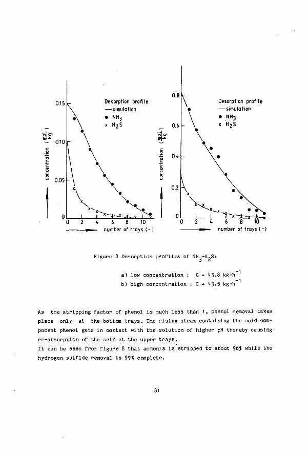
0.15

ol o*

Desorption profile — simulation • NH3

x H2S

Sr 0.10

0.05

n

i\

U 6 8 10 — number of frays (- )

Desorption profile — simulation • NH3

x H 2 S

2 l> 6 8 10 — m number of frays ( - )

Figure 8 Desorption profiles of NH,-H.S:

a) low concentration ; G • H3-8 kg»h b) high concentration ; G = ^3•5 kg-h

-1

As the stripping factor of phenol is much less than 1, phenol removal takes place only at the bottom trays. The rising steam containing the acid com­ponent phenol gets in contact with the solution of higher pH thereby causing re-absorption of the acid at the upper trays. It can be seen from figure 8 that ammonia is stripped to about 96$ while the hydrogen sulfide removal is 99% complete.

81

0.15 -

Ik o en E r 0.10

" 0.05 -

x

•\

L\ \

\

I

Desorption profile —simulation • NH3

♦ C02

\ •

\

i I I I

0 0.1 -

U 6 8 10 — number of frays ( - )

U 6 8 10 — number of trays (■

Figure 9 Desorption profi les of NH -CO :

a) low concentration ; G b) high concentration ; G

19.5 kg-h .' 15.6 kg-h ■1

For the ammonia-carbon dioxide mixtures in figure 9, NH s t r ipping drops to about 93? while C02 i s removed for 90$. Desorption of quaternary mixtures (see figure 10) indicates rather low s t r ipping performance for CO (about 87$) compared to H2S , which i s completely str ipped even before reaching the seventh t ray, and NH , which i s desorbed for about 99$.

82

number of trays (-) » — number of trays (-)

Figure 10 Desorption profi les of NH -H2S-C02:

a) low concentration j G = H9.5 kg'h . b) high concentration ; G = HI.6 kg-h .

For the experiment with rea l sour water the measured and predicted values agree quite well (figure 11). I t i s worth mentioning here that when the measured and simulated concentra­t ions are plot ted on a logarithmic sca le , differences do become v is ib le , par t i cu la r ly for the bottom concentrations of H2S. This would give, however, an u n r e a l i s t i c representat ion of the measurements.

83

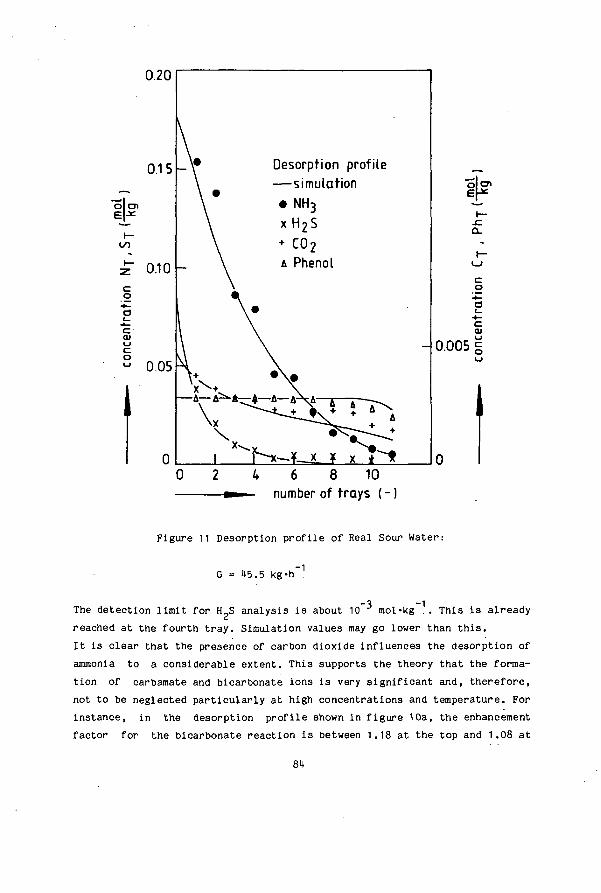
o en e-* on

c o

O)

0.20

0.15

0.10

0.05

0

_\»

\ •

i ' x V

—A— A^A-

Xv

I

Desorption profile —simulation • NH3

xH2S ♦ C02 A Phenol

\ » a A - \A ^

X * X

;|cn o -

c o

c aj

- 0.005

4 6 8 10 - number of trays (-)

Figure 11 Desorption profile of Real Sour Water:

G ■= H5.5 kg-h

-3 -1 The detection limit for H?S analysis is about 10 mol«kg .. This is already reached at the fourth tray. Simulation values may go lower than this. It is clear that the presence of carbon dioxide influences the desorption of ammonia to a considerable extent. This supports the theory that the forma­tion of carbamate and bicarbonate ions is very significant and, therefore, not to be neglected particularly at high concentrations and temperature. For instance, in the desorption profile shown in figure 10a, the enhancement factor for the bicarbonate reaction is between 1.18 at the top and 1.08 at

81

the bottom with a maximum of 1.24 at the third and fourth tray; the car-bamate reaction, on the other hand, contributes to the liquid mass transfer flux with enhancement factors between 2.20 at the top and 1.03 at the bottom with a maximum of 2.32 at the second tray. (A higher carbamate enhancement factor does not necessarily imply that its contribution to the C0_ flux is larger). I t can be concluded from these figures that good agreement between the experimental and simulated r e su l t s has been achieved. To t e s t the s ens i t i v i t y of the model to some parameters, the effect of parameter variat ions was analyzed. The parameters were:

(a) the steam r a t e , G (b) the l iquid phase mass transfer coeff ic ient , k. (c) the gas phase mass t ransfer coeff ic ient , k (d) the in te r fac ia l area, a

The sens i t i v i t y analysis was performed for the experiment shown in figure 10a where the feed composition i s NT=0.224 mol-kg . , S =0.077 mol«kg . and

-1 -1 -1

C =0.054 mol-kg . with L = 100 kg-h . and G = 19.52 kg-h . To simulate possible experimental errors in the steam r a t e measurements, the steam ra te was varied by 10%. For the mass t ransfer parameters, the uncertainty i s larger and the values were increased and decreased by 50?. Two "reference" points were used. One i s the model used where the calculated out le t con­centrat ions are: NT= 0.012473 mol-kg - 1 , ST= 0.000000 mol-kg""1, CT= 0.005690 mol-kg"1. The other uses the estimates of Nonhebel (1972) which are: k1= 6.9-10 - m»s~1, k = 3.1 '10~2 m-s"1 , afc = 0.39 m2. The Nonhebel values were used to i l l u s t r a t e the behaviour of H S when complete desorption would not take place out le t concentrations: N = 0.012651 mol-kg"1, S - 0.000167 mol-kg"1, C?= 0.019614 mol •kg - 1 . The r e su l t s of these analyses are summarized in table 3. The percentages indicated are the r a t i o of the deviation of the effluent concentrations ( i . e . the "reference" minus the "variable" to the "reference" effluent concentrat ions) . The minus sign indicates poorer s t r ipping performance with respect to the "reference" taken. The values for H?S indicated by the sign ii—ii should be read as values having no physical relevance because the absolute values for a l l ca lcula t ions approach zero. Thus the comparison of these values depends on the number of s ignif icant d ig i t s (larger than 6) one may wish to consider. For the Nonhebel ca lcu la t ions , percentages were based on the difference up to 6 s ignif icant f igures .

85

Table 3. Sensitivity Analysis. Percent Deviation

Parameter Component 50% decrease 50Ï increase Model Nonhebel Model Nonhebel

NH3

co„

NH H2S co„

NH H 2 S

C0„

NH H2S C0„

- 65 —

- 91

- 25 —

- 13

-111) —

-151

10% Model

-36 —

-21

- 31 -568 - 16

- 51 -710 - 8

- 89 -1510 -82

decrease Nonhebel

-15 -81 - 5

26 — 31

5 — 2

37 — 17

10% Model

23 — 17

16 18 25

17 60 6

37 81 37

increase Nonhebel

11 36 -5

86

The results are rather complicated to analyze because all parameters are to a certain extent dependent on each other. Some general conclusions can however be drawn: (1) The model is more sensitive to the decrease of the parameter values than to increasing them. This is because changes in the mass transfer parameters subsequently change the number of (overall) transfer units. This influences the overall Murphree efficiency which contains the number of transfer units in the exponential term making it more susceptible to decreases than to increases; (2) The most sensitive among the components is H i ; (3) Variations of the k. indicate considerable changes for all components; (H) Variations of the k affect the desorption of NH., and HJ3 more

g 3 2 remarkably than that of C0_ ; (5) It is obvious that changing the interfacial area will alter stripping performance regardless of the set of mass transfer coefficients used. From the these observations it can be deducted that for C0p the mass trans­fer resistance lies in the liquid phase. For NH, and H.S, mass transfer is sensitive to both the k, and k .

1 g 7. COMPARISON BETWEEN PREDICTED AND REPORTED PERFORMANCE

We have also attempted to check the model against existing data from sour water strippers. The operating data wre taken from a report by the Americam Petroleum Institute (API, 1972). None of these sets of data was found to be complete. In particular no C0? concentrations are given. Of the strippers we have tried out H are refluxed and 5 non refluxed. In the API report, mass transfer coeficients are not given for the par­ticular strippers. To make an estimate of these coefficients, the relations of Nonhebel were used. These relations were used for the following reasons: - they give values which are roughly in the middle in the range given by different authors (see figure H). - the Nonhebel relations for k, and k are relatively simple; the

1 g coefficients are assumed to depend only on diffusion coefficient. As a consequence, they are nearly equal for all strippers operating at a temperature of about 100 °C.

- the Nonhebel relations do not require information about the lay out of the tray or other unknowns.

87

Table 1 . Results of the s imula t ion of the s t r ippers from the API r e p o r t .

s t r i p p e r nr 14 21a 27 31 11 17 18 51a

number of trays 6 15 10 8 16 19 12 5

feed (kg-h~1) 17370 87503 55368 15851 86852 10857 17370 10857

steam (kg-h _ 1 ) 2064 5113 12111 2631 10251 2510 1950 511

temp, top 112 130 121 110 110 110 110 107

(°C) bottom 116 133 138 111 116 111 113 110

cond 106 - 79 77 -

press, top 156 276 237 118 167 109 111 129

(kPa.) bottom 175 296 312 163 175 129 159 113

a.. . . . (m2) 30.8 55.7 60.2 33.9 91.5 12 .5 ' 21.8 8.3 Nonnebel . . . .

N_ , . mol-kg"1 .07086 .11800 .11812 .32090 .08269 .05900 .06181 .01266 T.feed . . .

S T f e e d .05901 .01176 .12582 .65800 .05020 .07530 .00633 .01230 Ph. . .00619 .00622 .00321 .00251 .01011 .00587 - .00021 feed . . . .

N cal.c. .01932 .01618 .05877 .00670 .05981 .00007 .00219 .00717 rep. .01672 .01762 .01177 .02401 .02356 .00676 .00677 .00447

ST bot ° a l 0 - - 0 0 150 .00191 .00322 .00041 .00381 .00000 .00008 .00111 rep. .00008 .00260 .00059 .00038 .00589 .00015 2- .00018

PhT bot C a l C' -00577 -00582 3x .00189 3x .00369 - .00020 rep. .00620 .00510 .00160 .00033 .00639 .00239 - .00011

- not present

'aNonhebel = 37.9 m2, see text 2 - not measured 3x not calculated, see t e x t .

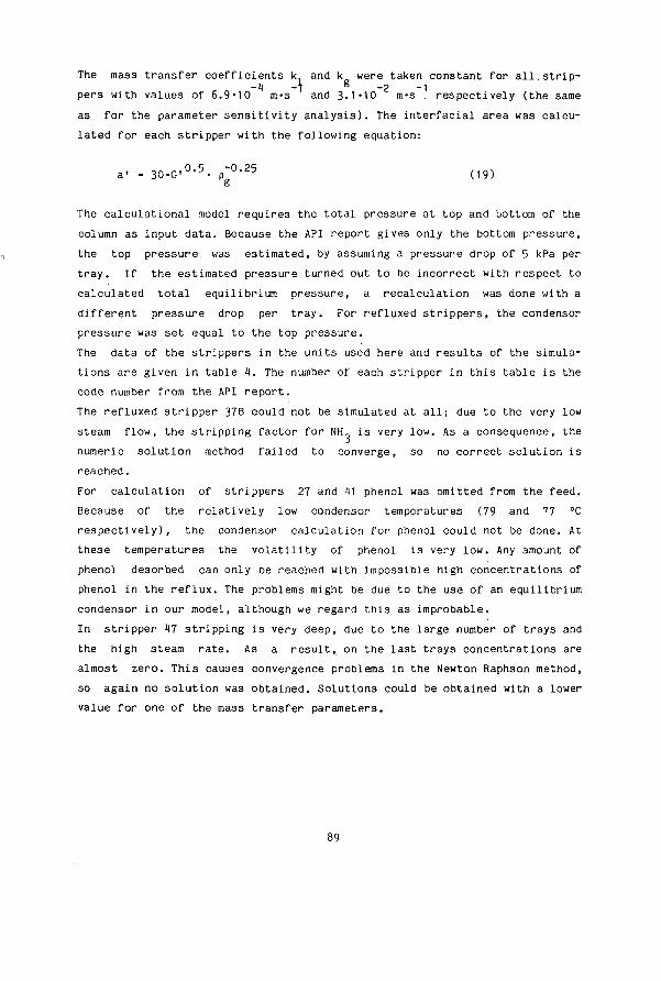
The mass transfer coefficients k. and k were taken constant for all.strip--i) -'T 8 -2 -1 pers with values of 6.9*10 m-s . and 3.1-10 m-s . respectively (the same

as for the parameter sensitivity analysis). The interfacial area was calcu­lated for each stripper with the following equation:

a- - 30-G'0-5. p-°-25 (19)

The calculational model requires the total pressure at top and bottom of the column as input data. Because the API report gives only the bottom pressure, the top pressure was estimated, by assuming a pressure drop of 5 kPa per tray. If the estimated pressure turned out to be incorrect with respect to calculated total equilibrium pressure, a recalculation was done with a different pressure drop per tray. For refluxed strippers, the condensor pressure was set equal to the top pressure. The data of the strippers in the units used here and results of the simula­tions are given in table 1. The number of each stripper in this table is the code number from the API report. The refluxed stripper 37B could not be simulated at all; due to the very low steam flow, the stripping factor for NH. is very low. As a consequence, the numeric solution method failed to converge, so no correct solution is reached. For calculation of strippers 27 and 11 phenol was omitted from the feed. Because of the relatively low condensor temperatures (79 and 77 °C respectively), the condensor calculation for phenol could not be done. At these temperatures the volatility of phenol is very low. Any amount of phenol desorbed can only be reached with impossible high concentrations of phenol in the reflux. The problems might be due to the use of an equilibrium condensor in our model, although we regard this as improbable. In stripper 17 stripping is very deep, due to the large number of trays and the high steam rate. As a result, on the last trays concentrations are almost zero. This causes convergence problems in the Newton Raphson method, so again no solution was obtained. Solutions could be obtained with a lower value for one of the mass transfer parameters.

89

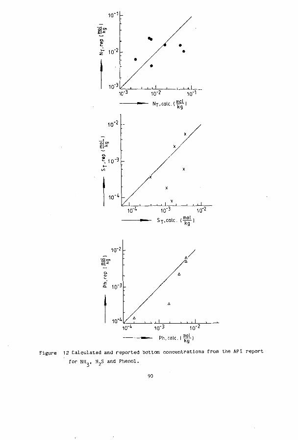
10

10'

-1

"2

"3

■ •

■

«to

/ •

, , 1

• •

1 r i l l

1 0 " -

10' -3

10 -2

e-"

■-. 10"

10"

10~* NT.calc.(^:

10"

_i L J l ' ' ' 10' 1-4 10"3

ST,CDtc. ( 10' f2

mol kg

— Ph.aUc.lf) Figure 12 Calculated and reported bottom concentrations from the API report

for NH , HpS and Phenol.

90

Because the mass transfer rates are the most sensitive to a change, in the interfacial area, this parameter was set to a lower value.

2 While the Nonhebel equation predicts an interfacial area of 37.9 m per 2 tray, a solution could only be reached for values of 12.5 m per tray or

less. All other strippers were simulated without problems. The results from table 1 have been plotted in figure 12. For all components considerable deviations are seen between calculated and reported concentrations. To these conclusions the following remarks can be made: - The mass transfer parameters are not well known, but estimated with gene­ral correlations. If more accurate values for these parameters were known, better agreement between calculated and reported bottom concentrations could possibly be obtained. No attempt was undertaken to optimize the results.

- The presence of CO is not regarded in the API report, although it usually is present in sour water in a concentration that is about one half of the concentration of HpS (figure 11, Darton et al., 1978). C0? substantially influences the stripping of the other components: NH, is stripped less easily in the presence of C0_, H.S and phenol are stripped more easily. Our model can take into account the effects of C0?, so if information of the concentration CO in the feed would be available, better agreement could be reached for the other components. - The reported stripping performances for phenol are remarkably high. For equilibrium stages, the maximum fraction of a component that can be stripped for a large number of (theoretical) trays is equal to the stripping factor if this factor is less than unity. However, in most cases, the reported stripping is much deeper than this maximum theoretical value. For this fact there are several possible explanations: a) the reported concentrations of phenol may be erroneous ; this could be

caused by analytical problems, because determination of phenol in water is rather difficult.

b) the equilibrium constant and/or Henry constant of phenol we have used may be erroneous; however, they give results that are in reasonable agreement with our experiments.

c) the reported concentrations could be the sum of concentrations of various phenolic components. Of these related compounds, most are more volatile than phenol itself in aqueous media, so total removal can be better than calculated for pure phenol.

91

- The data in the API report are average values of plant data; in general, plant data are less accurate than experimental data, obtained from laboratory data.

Overall it would appear that existing data on plant operation are not suffi­ciently well documented to allow a comparison with our model.

8. STAGE EFFICIENCIES

In sour water strippers, the stage efficiency has a different value for each component. Because the efficiencies show a complicated dependency of the system and its parameters, they cannot be exactly predicted. In our calcula-tional model, stage efficiencies can be determined afterwards from the calculated concentrations in the gas and liquid phase. In the following parts, the applicability of two different stage ef­ficiencies, the Murphree stage efficiency and the vaporization efficiency, to sour water strippers will be evaluated.

8.1. MURPHREE STAGE EFFICIENCY

A widely used efficiency is the Murphree stage efficiency, calculated for the gas phase. This efficiency is defined as:

. yout " y m ( mv, i *

y - y. ' 'in

Here y is the concentration in the gas phase, in equilibrium with the bulk of the liquid. A similar equation exists for the Murphree stage efficiency for the liquid phase. In this case, concentrations in the gas phase (y) are substituted by concentrations in the liquid phase (x). For separation of hydrocarbon mixtures by distillation, or pure physical desorption, the Murphree gas stage efficiency is commonly used. The ef­ficiency is either recalculated for each tray or taken constant over the whole column. This approach can give good results for some kind of systems (AIChE, 1958). To find out if the Murphree stage efficiency concept is applicable to sour water strippers, the efficiencies were calculated at each stage of various strippers.

92

From these calculations, it became clear that the Murphree stage efficiency is different for every component. For NH , the efficiency usually has a value between 0.65 and 0.85, for H-S between 0.15 and 0.4. For C0_ and phenol, efficiencies vary from 0.01 to 0.05 and from 0.65 to 0.9 repectively. These figures are in agreement with the Henry coefficients of the components. However, the Murphree stage efficiency of each component is not constant over the whole column; especially in the top section, large variations are encountered.

Table 5. E .,,, and N„ for one of our experiments (see figure 8a) mv.NH, T -1 -1

Concentrations in the feed: N 0.149 mol-kg , S_ 0.108 mol-kg Concentrations in the table are concentrations in the liquid, leaving the tray.

G (kg^h ') 43.8 40.0 30.0

tray T mol -kg

NT mol«kg -1

1 mol-kg -1

eed

1

2

3 4

5 6

7 8

9 10

11

-14.866

0.963

0.819

0.787 0.774

0.768

0.765 0.764

0.763

0.763 0.764

.14900

.13604

.11557

.09281

.07275

.05592

.04211

.03094

.02197

.01480

.00908

.00453

--0.648

1.057 0.852

0.812

0.798

0.791 0.788

0.787 0.786

0.786

0.786

.14900

.14391

.12911

.10968

.09085

.07366

.05842

.04509

.03355

.02360

.01506

.00773

-0.496 0.156

1 .185

0.913 0.869

0.855

0.849

0.847

0.846

0.846

0.846

.14900

.16080

.16245

.15728

.14878

.13787

.12492

.11006

.09329

.07453

.05368

.03060

93

In some cases the efficiency for NH., can have a value less than zero or greater than unity. This possibility is also observed in multicomponent mass transfer without chemical reaction (see Krishna and Taylor, 1986). The appearance of these strange values, which have nothing to do with the hydrodynamics of the , tray, will be explained later on. For the other com­ponents, the efficiency is always between zero and unity. As an illustration of the behaviour of the Murphree stage efficiencies as a function of the position in the column, table 5 gives a calculated ef­ficiency and simulated concentration profile for NH_. These values are calculated for the feed composition of one of our experiments with NH and H.S only (figure 8a). The calculation was done for various steam rates. In this table the variation of the efficiency over the first trays of the column can be seen. For H?S, the Murphree stage efficiency is also far from constant over the column. In the first and second case in table 5, the concentration of N-, in the liquid decreases on each tray. In the third case, a concentration increase is observed on the first two trays. This means that NH,, desorbed in the bottom section, is absorbed again in the top. This effect occurs at low steam rates, so with relatively high concentrations of ammonia in the gas. At the top trays this gas concentration can be higher than the equilibrium pressure of ammonia because this is lowered by the presence of hydrogen sulphide. This results in absorption of ammonia, due to the negative driving force for ammonia desorption. From table 5 it can be seen that it is not possible to say from the value of the Murphree stage efficiency if stripping or absorption takes place at a particular tray. In this table, stripping is encountered for values of E , ranging from -0.65 till 11.9, while absorption takes place at 2 trays where E , is 0.50 and 0.16 respectively. mv,i To explain this, it is necessary to take a look at the physical meaning of the different values of the Murphree stage efficiency. All possible situa-tions with different values for y. , y and y are depicted in figure 13, which is a convenient representation of equation 19. In this figure, absorp­tion cases are indicated as A1 , A2 and A3, desorption as D1 , D2 and D3. It is clear that for every value of the efficiency, both ab- and desorption can occur. Which one of the two takes place is determined by the difference y . - y. only. From now on, only desorption will be discussed; for absorp­tion, analogous discussions can be made.

91

MV y * - y i n

A1' .fout WjA

A2

--8

A3

fy-m

—« U

D2

D3

--8

yout

E M V < 0

yin

It 0 « E M V

< 1

E M V > 1

Figure 13 Schematical drawings of the physical meaning of different values for E . Cases are depicted for both ab-mv . Bar in y . denotes the magnitude of y, for E . Cases are depicted for both ab- (A) and desorption (D).

From figure 13 turns out that, if y is small, that is less then y. the * ln

efficiency has a negative value (D1). If y lies in the particular range between y. and y f, the value of E becomes larger then unity (D3). If w 1.11 Uv*v UiVpX

y is larger then y , the efficiency ranges from zero to unity. The value of y depends on the values N_ and S„ (roughly y = He.,„-(N„-S„)). u 1 1 Nn 3 1 1 So y can have such a value that one of the 'particular' cases D1 or D3 is reached. In the bottom section, where S„ is low, the column behaves as a physical ammonia stripper. The value of the efficiency can than be calcu­lated from the mass transfer parameters, enhancement factor and the gas velocity. From the forgoing considerations it is clear, that the Murphree stage ef­ficiency can not be used succesfully for the calculation of sour water stripping, because this efficiency is not constant and can not be predicted for each situation at forehand.

95

8.2. VAPORIZATION EFFICIENCY

To avoid the problems, caused by the use of the Murphree stage efficiency, Won (1983) proposed to use the vaporization efficiency, defined by Holland (1970) as:

h . yactual.l ( 2 0 )

yi

Won took the vaporization efficiency as constant over the column, but with a different value for each component. For 1 strippers from the API report (1973), 2 refluxed and 2 nonrefluxed, the component efficiency was deter­mined by fitting on the bottom concentration. The form of the concentration profile was not taken into account due to lack of information. The descrip­tion of sour water strippers with a vaporization efficiency is the best method known until now. Besides the effect of making the stripping calculation more comprehensive, the use of the vaporization efficiency has a second advantage. The mass transfer model is based on a numeric solution of the total set of equations, which requires a large calculation time (e.g. for 1 components on a VAX 750 computer, calculation takes about 5 minutes). It is an iterative process with iterations at 3 levels. The second level is an iteration loop on a tray, which is repeated until the mass balances of that tray are satisfied. Usually, this loop is performed 3 or H times per tray. However, each loop requires two mass transfer calculations for one component, three for two components and so on. As a consequence, the calculation is accelerated by a factor of 6 to 20 if the second iterative loop is replaced by a pseudo equilibrium calculation with the use of the vaporization efficiency. The stripping performance of the particular tray is now described by a set of equations that can be solved analytically. In our model, the vaporization efficiencies have been calculated from the concentrations in the gas phase. To obtain a value for the vaporization efficiency of each component over the column, the arithmetic mean efficiency was calculated. However, it seems likely that the larger the concentration difference (y - y ) on a tray, the more important the efficiency of that tray will be. To account for this fact, a concentration dependent mean efficiency was also calculated, defined as:

96

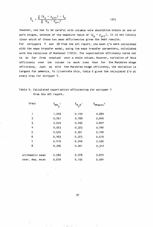
7 " ( y " ' C i = £ (y n w n w

V i ' (21)

However, one has to be careful with columns were absorption occurs at one or more s t ages , because of the negative value of (y - y ) . I t i s not to t a l ly c lear which of these two mean eff ic iencies gives the best r e s u l t s . For s t r ippers 7 and 58 from the API repor t , the mean C's were calculated with the mass t ransfer model, using the mass transfer parameters, calculated with the r e l a t i ons of Nonhebel (1972). The vaporization efficiency turns out to be far from constant over a whole column. However, var ia t ion of th is efficiency over the column i s much l e s s than for the Murphree stage eff ic iency. Ju s t as with the Murphree stage efficiency, the var ia t ion i s l a rges t for ammonia. To i l l u s t r a t e t h i s , table 6 gives the calculated g 's at every t ray for s t r ipper 7.

Table 6. Calculated vaporization eff ic iencies for s t r ipper 7 from the API repor t .

t r a y : NH„ H 2 S Phenol

1 2 3 4 5 6 7 8

arithmetic cone. dep.

mean mean

1 .046 0.701 0.609 0.563 0.526 0.1)83 0.118 0.296

0.580 0.679

0.100

0.189

0.265

0.323

0.361

0.373

0.349

0.261

0.278

0.150

0.881 0.846 0.807 0.760 0.700 0.619 0.500 0.312

0.679 0.564

97

With these £'s, the pseudo equilibrium calculation was performed, again for NH and H?S only. To simulate strippers by pseudo equilibrium calculations with the vaporization efficiency, a modified version of our own computer program was developed. In this version, the mass transfer equations were replaced by equilibrium calculations. At each tray, the composition of the liquid leaving was calculated from the composition of the leaving gas. From the mass balance for every component at the particular tray, the composition of the entering gas was found. The auxiliary calculations, such as calcula­tion of the total liquid and gas flow, gas density and equilibrium con­stants, are exactly the same as in our own model. With this model, the calculations of Won for nonrefluxed strippers (nr 7 and 58) were checked. Phenol was omitted from the feed because of convergence problems. Results of these calculations are given in table 7 as case 2. The calculated bottom concentrations of both NH and H.S were too low by a factor of 2.6 for stripper 7 as compared to the results reported by Won. For stripper 58, calculated bottom concentrations were too low by a factor H.H

and 5.9 for NH and H.S respectively. However, when the stripping perfor­mances are compared instead of the bottom concentrations, differences are much smalller. It is not clear what is the cause of the differences between calculated and reported concentrations. A possible reason is the thermodynamic model used. Won used the computer program DELTAS, which is based on the model of Edwards et al. (1978). Our model is based on the same equations, with the revised parameters given by Maurer (1980). As discussed above the minor differences between the two sets of parameters can give astonishingly large differences in the calculated equilibria. The calculation of stripper 7 with the concentration dependent mean ef­ficiency clearly illustrates the influence of the stripping performance of one component on the other. The calculated efficiency for H_S is equal to the value reported by Won. However, with the slightly lower efficiency for NH.,, and thus less deep stripping of ammonia, the bottom concentration of H S has also increased. From table 7 and other calculations, the following conclusions can be drawn: - Mean value of the vaporization efficiency over the whole column depend on almost all input parameters of the model, like temperature and pressure of the column, liquid and gas flow rates, composition of the feed and mass transfer parameters.

98

Table 7. Calculated and reported vaporization efficiencies and bottom concentrations calculated with these efficiencies.

Case 1: C's and c. reported by Won Case 2: £'s reported by Won, c. ,. calculated Case 3= concentration dependent mean E's, c. . calculated

bot Case iJ: a r i thmet ic mean E's , c. . calculated

bot Case 5: c,_ . calculated with mass transfer model bot Case:

stripper

5NH CH2S

NT,bot T.bot

stripper

SlH 5H2S

T.bot ^T X„l-

7

58

0.7

0.15

0.00353 0.00082

0.65

0.20

0.00059 0.000017

0.7

0.15

0.00134 0.00031

0.65

0.20

0.00011 0.000008

0.68

0.15

0.00156 0.00035

0.65

0.37

0.00009 0.000001

0.58

0.28

0.00186 0.00022

0.62

0.13

0.00012 0.000001

-

" 0.00261 0.00021

-~

0.00012 0.000001

T.bot

These influences make it impossible to calculate the vaporization efficiency exactly at forehand. On the other hand, a change in £ gives only moderate differences in the bottom concentrations, so a small error in the ef­ficiencies used does not have very much influence on the total stripping performances. -For all components, calculated mean vaporization efficiencies can differ from those reported by Won (1983). Won gives a figure from which the value of the vaporization for each component can be estimated from the partition

99

coefficient of the component and the kinematic viscosity of water. As discussed above this is a too simple representation of the true phenomena. -The vaporization efficiency can be larger than unity. This is possible if the concentration of a component in its molecular form is larger at the interface than in the bulk of the liquid. -It is not possible to determine from the value of the vaporizaton effiency whether absorption or desorption at a particular tray takes place. -For strippers 7 and 58, the change in the calculated bottom concentrations, caused by a change in the vaporization efficiency, is rather small. In fact, these changes are much smaller than the difference between bottom concentrations calculated and those reported by Won. -In most cases, the arithmetic mean vaporization efficiency gives somewhat better agreement with the mass transfer model than the concentration dependent mean efficiency. A final remark on made to the form of the concentration profile, determined by pseudo equilibrium calculations. From our calculations it turns out that, in some cases, this form differs significantly from the one calculated with the mass transfer model. As an example, concentration profiles for the refluxed stripper 11 from the API report, calculated by both mass transfer and pseudo equilibrium calculations, are plotted in figure 11. Because the stripper is refluxed, feed concentrations depend on the total stripping performance and so are different in both cases.

100

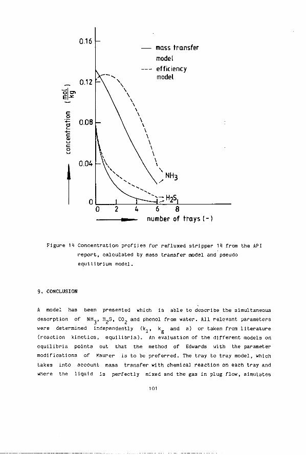
0.16

_ 0.12 -

il-?

''S 0.08 c

mass transfer model efficiency model

0.04 - \ \

0 2 4 6 8 ■ number of trays (-)

Figure 1H Concentration profiles for refluxed stripper 11 from the API report, calculated by mass transfer model and pseudo equilibrium model.

9. CONCLUSION

A model has been presented which is able to describe the simultaneous desorption of NH,, H S, CO and phenol from water. All relevant parameters were determined independently (k. , k and a) or taken from literature (reaction kinetics, equilibria). An evaluation of the different models on equilibria points out that the method of Edwards with the parameter modifications of Maurer is to be preferred. The tray to tray model, which takes into account mass transfer with chemical reaction on each tray and where the liquid is perfectly mixed and the gas in plug flow, simulates

101

measured values quite well for both "synthetic" and real sour water. This indicates that the mass transfer parameters used describe the system under consideration well. This would have not been possible when literature values were used. Comparison of the model and results from industrial strippers is less satisfactory. The most difficult problem for calculating industrial type strippers are the values of the mass transfer coefficients and interfacial area. Existing correlations show enormous differences and are clearly unreliable. Unfortunately column performance depends rather strongly on the mass transfer parameters. The use of efficiencies has to be avoided, because their definition has no (physical) meaning in desorption with a chemical reaction. This was shown to hold for both Murphree and vaporization efficiency. The model used has described the condensor and reboiler of a stripper as an equilibrium stage. A furthur refinement could be introduced by modelling these stages in a more realistic way. As the condendonsor performance in­fluences the whole unit, the condensor model is not unimportant. The application of our model to packed column operation was not investigated. It is possible to change the model presented to simulate a packed column. Basically the same equations can be used if plug flow is assumed for both liquid and gas. In how far non ideal flows patterns (such as investigated by Hoek, 1987) would be important is however uncertain.

ACKNOWLEDGEMENTS

The autors would like to thank R.C. Darton and P.F.A. van Grinsven from the Koninklijke Shell Laboratorium Amsterdam for their contribution to the set up in this work and their cooperation to provide the refinery sour water.

102

10. SYMBOLS

a interfacial area per unit dispersion volume m 2

a. total interfacial area per tray m a' interfacial area per unit bubbling area B weir length m

2 BA bubbling area m C. liquid concentration mol C gas concentration mol g C„ total carbon dioxide concentration mol D„ column diameter m

2 D gas diffusion coefficient m • g 2 D. liquid diffusion coefficient m • d perforation diameter m E„„_ enhancement factor due to HCO, reaction (-) nL.U3 5 EMU n™ enhancement factor due to NH„C00 reaction (-) E„ . .. total enhancement factor for CO. (-) C.tot 2 E . Murphree stage efficiency for component i (-) F percent free area of the plate (-) G vapor load kg-G' vapor load per unit cross-sectional area kg»

2 g acceleration of gravity m • Hau„_ Hatta number for HCO., reaction (-) HOU 3 j Ha«.u ™ « Hatta number for NH„C00 reaction (-) Nn2OUU c Hf froth height m H tray spacing m H weir height m w He Henry's constant atm h. clear-liquid height or hold-up m J flux mol K equilibrium constant * K pseudo equilibrium constant (-) k liquid phase mass transfer coefficient m'S k gas phase mass transfer coefficient m-s g kn reaction rate constant kg • k„„ reaction rate constant kg-Nn 3 L liquid rate kg •

103

L' liquid rate per unit cross-sectional area N number of gas phase transfer units, k a'/u g g g

N total ammonia concentration n number of perforations P pressure p pitch Ph total phenol concentration S. stripping factor of comp. i S„ total hydrogen sulphide concentration Sc Schmidt number T temperature x liquid concentration y gas concentration *

y gas concentration in equilibrium with the other

phase

(* depends on the reaction involved) Greek

6 interaction parameter (-) n gas viscosity Pa-s g tl. liquid viscosity , Pa-s

- 2 kg-m -s

(-) mol-• k g " 1

Pa o r mm

m

mol

(-) mol

• k g " 1

• k g " 1

K o r °C

mol

mol

mol

• k g ' 1

, - 1 •kg - 1

•kg

-3 p gas density kg-m 8 -3 p. liquid density kg>m 1 -1 o surface tension N»m £. vaporization efficiency for component i (-) 0 residence time of gas in froth zone s

104

subscript

b bulk calc calculated cond condensor exp experimental g gas int interface 1 liquid n tray number rep reported

105

11. LITERATURE

American Institute Of Chemical Engineers, 1958, Tray Efficiencies In Distillation Columns, Final Report from the University of Delaware, AIChE.New York. American Petroleum Institute, 1973, 1972 Sour Water Stripping Survey Evaluation, Publication No. 927, Washington D.C.. Asano K., Fujita S., 1966, Liquid-Phase Mass Transfer Coefficients In Tray Towers, Kagaku Kogaku, 1, 330-334. Asano K., Fujita S., 1966, Vapour-Phase Mass Transfer Coefficients In Tray Towers: A New Method For Prediction Of Tray Efficiency, Kagaku Kogaku, 4, 369-375. Beutier D., Renon H., 1978, Representation Of NH -H S-H20, NH -C02~H20, NH -SO -H.0 Vapor Liquid Equilibria, Ind.Eng.Chem.Process Des Dev., 17, 3, 220-230. Blauwhoff P.M.M., Kamphuis B., van Swaaij W.P.M., Westerterp K.R.,1985, Absorber Design In Sour Natural Gas Treatment Plants: Impact Of Process Variables On Operation And Economics, Chem.Eng.Process., 19, 1-25. Calderbank P.H., Moo-Young M.B., 1961, The Continuous Phase Heat And Mass Transfer Properties Of Dispersions, Chem.Eng.Sci., 16, 39-54. Cornelissen A.E., 1980, Simulation Of Absorbtion Of H-S And COp Into Aqueous Alkanolamines In Tray And Packed Columns, Trans. IChem. E., 58, 212-250. Coulson J.M., Richardson J.F., 1978, Chemical Engineering, Volume 2, Pergamon Press,London, 511.

Danckwerts P.V., 1975, Gas Liquid Reactions, Mc-Graw Hill, New York. Darton R.C., van Grinsven P.F.A., Simon M.M., 1978, Development Of Steam Stripping Of Sour Water, Chem. Eng. (London), 339, 923-927. Edwards T.J., Maurer G., Newman J., Prausnitz J.M.,1978, Vapor Liquid Equilibria In Multicomponent Aqueous Solutions Of Volatile Weak Electrolytes AIChE J., 21, 966-976.

Gmelins Handbuch der Anorganischen Chemie, Baczko von K. editor, Gmelin-Institut / Gesellschaft Deutcher Chemiker, Verlag Chemie GMBH, Weinheim.

Hoek P.J., Wesselingh J.A., Zuiderweg F.J., Small Scale And Large Scale Maldistribution In Packed Columns, accepted for publication in Chem. Eng. Res. & Dev. Holland CD., McMahon D.S., Comparison Of Vaporisation Efficiencies With Murphree-Type Efficiency In Distillation -I, 1970, Chem. Eng. Sci., 25,

106

131-136. Hoogendoorn G.C. et al. (submitted for publication to Chem.Eng.Sci.) Krevelen D.W van, Hoftijzer P.J., Huntjens F.J., 19^9, Composition And Vapour Pressures Of Aqueous Solutions Of Ammonia , Carbon Dioxide And Hydrogen Sulphide, Rec. Trav. Chim. Pays-Bas, 68, 191-216. Krishna R., Taylor R., 1986, Handbook of Heat and Mass Transfer, Gulf Publishing Company, Houston, 259-132.

Maurer G., 1980, On The Solubility Of Volatile Weak Electrolytes In Aqueous Solutions, in Thermodynamics of Aqueous Systems with Industrial Applications, ACS Symposium Series 133, 139-172, American Chemical Society Washington D.C.. Nonhebel G., 1972, Gas Purification Processes for Air Pollution Control Butterworth & Co., London, 105-107. Pawlikowski E.M., Newman J., Prausnitz J.M., 1983, Vapor Liquid Equilibria For NH and H O in The 100 to 150 °C Region: Effect Of Low Levels Of Phenol On Partial Pressure of Ammonia, AIChE J., 29, 5, 869-871.

Perry R.H., Green D.W., 1981, Chemical Engineers' Handbook, Sixth Ed., Mc Graw Hill New York, 18/5-18/16 Pinsent B.R.W., Pearson L., Roughton F.J.W., 1956a, The Kinetics Of Combination Of Carbon Dioxide With Hydroxide Ions, Trans. Faraday S o c , 52, 1512-1520. Pinsent B.R.W., Pearson L., Roughton F.J.W., 1956b, The Kinetics Of Combination Of Carbon Dioxide With Ammonia, Trans. Faraday Soc, 52, 1591-1598. Treybal R.E, 1981, Mass Transfer Operations, Third Ed., Mc Graw-Hill, New York, 183-

Tsonopoulos C , Coulson D.M., Inman L.B., 1976, Ionization Constants Of Water Pollutants, J. Chem.Eng.Data, 21, 190-193. Wilson G.M., 1978, A New Correlation Of NH-, CO and H S Volatility Data from Aqueous Sour Water Systems, Final Report To API Committee on Refinery Environmental Control Under EPA Grant NO. R801361010, Thermoehemieal Institute, Brigham Young Univ, Provo, Utah. Won K.W., 1983, Sour Water Stripper Efficiency, Plant Operations Progress, 2, 108-113. Zuiderweg F.J., 1982, Sieve Trays -A View Of The State Of The Art-, Chem.Eng.Sci., 37, 1111-1161).

107

ABSTRACT

This thesis is a comprehensive study of the simultaneous removal of volatile weak electrolytes such as ammonia, hydrogen sulphide, carbon dioxide and phenol from aqueous wastes. Experiments have been carried out with various solutions of the electrolytes in a wetted wall column and try column. In the wetted wall column air was used as a stripping agent; in the tray column steam was used. A relative simple model has been developed that predicts the desorption rate of each component provided the hydrodynamics of gas and liquid phase are known. In this model the chemical equilibria, diffusion and reaction rates are taken into account. This model is a considerable improvement on existing descriptions of sour water stripping operation. The experiments and calcula­tions have given a clear insight in the theory of desorption with chemical reaction concerning from the above mentioned solutions. The application of the model to industrial desorption columns is possible. The gas and liquid mass transfer coefficients and interfacial area should then be known accurately.

108

SAMENVATTING

Dit proefschrift behandelt de gelijtijdige desorptie van ammoniak, zwavel­waterstof, kooldioxide en fenol uit waterige oplossingen. Experimenten met diverse oplossingen van genoemde stoffen zijn uitgevoerd in een nattewand-kolom en in een schotelkolom. In de natte wand-kolom werd lucht als stripmedium gebruikt; in de schotelkolom werd met stoom gestript. Er is een model ontwikkeld dat de stofoverdrachtssnelheid van iedere com­ponent bij gegeven stromingscondities uitrekent. In dit model zijn de chemische evenwichten, diffusie- en reactiesnelheden van de verschillende componenten meegenomen. Dit model is een verbetering tegenover bestaande beschrijvingen van stofoverdrachtssnelheden. De experimenten aan beide kolommen hebben een duidelijk inzicht gegeven in de theorie van desorptie met chemische reactie. Toepassing van het ontwikkelde model op industriële desorptie kolommen is zeer goed mogelijk. De vloeistof en gas stofoverdrachtscoefficienten en het specifiek fasengrensvlak dienen dan voor een nauwkeurige voorspelling goed bekend te zijn.

109

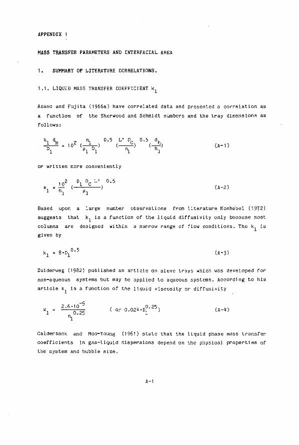
APPENDIX 1

MASS TRANSFER PARAMETERS AND INTERFACIAL AREA

1. SUMMARY OF LITERATURE CORRELATIONS.

1.1. LIQUID MASS TRANSFER COEFFICIENT k.±

Asano and Fujita (1966a) have correlated data and presented a correlation as a function of the Sherwood and Schmidt numbers and the tray dimensions as follows:

k. d. „ n 0.5 L' D 0.5 d

or written more conveniently

102 Dl °C L' °'5 k = 1° (-i-£ ) (A-2) l hx Pl

Based upon a large number observations from literature Nonhebel (1972) suggests that k. is a function of the liquid diffusivity only because most columns are designed within a narrow range of flow conditions. The k is given by

kl = 8-D!0'5 (A-3)

Zuiderweg (1982) published an article on sieve trays which was developed for non-aqueous systems but may be applied to aqueous systems. According to his article k is a function of the liquid viscosity or diffusivity

k. - 2-("\°Z ( or 0.024.D1°-25) (A-4) 1 U.<o 1

Calderbank and Moo-Young (1961) state that the liquid phase mass transfer coefficients in gas-liquid dispersions depend on the physical properties of the system and bubble size.

A-1

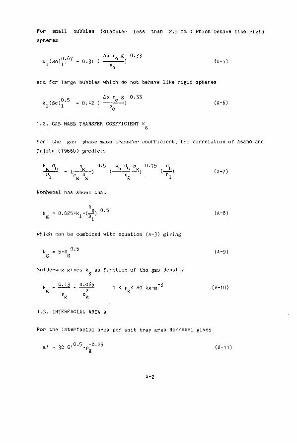
For small bubbles (diameter less than 2.5 mm ) which behave like rigid spheres

n fi7 Ap n g 0.33 k^Sc),- 0' = 0.31 ( — ) (A-5) 1 1 P„

and for large bubbles which do not behave like rigid spheres

0 5 AP nc g 0.33 k.(Sc), = 0.12 ( — ) (A-6) 1 1 P„

1.2. GAS MASS TRANSFER COEFFICIENT k g

For the gas phase mass transfer coefficient, the correlation of Asano and Fujita (1966b) predicts

k d. n 0.5 w. d. p 0.75 d. g h = ( S_) ( h h 8) (_Ü) (A-7)

1 g g g ' 1

Nonhebel has shown that

k = 0.625-kn .(^) °-5 (A-8)

g 1 01

which can be combined with equation (A-3) giving

k = 5-D °-5 (A-9) g g

Zuiderweg gives k as function of the gas density k _ 0^3 „ 0,065 1 < p < 80 kg.m-3 (A.10) 8 P P 8

g g 1.3. INTERFACIAL AREA a

For the interfacial area per unit tray area Nonhebel gives

a- =30G-°- 5.p-°- 2 5 (A-11) s

A-2

We interpret tray area as bubbling area. Zuiderweg reports for the mixed and emulsion flow regime

13 \ pg hl * °-53

F0.3 o

whereas for the spray regime

a' = - ^ - ( — § g 1 ) (A-13) p0.3 o

For the definition of these regimes the reader is advised to consult the article of Zuiderweg.

1.1. VOLUMETRIC LIQUID MASS TRANSFER COEFFICIENT ^ a

According to Perry's Chemical Engineers Handbook (1981), which is based on the AIChE Report (1958)

k.a = ( 3.875-108 D.)°-5( 0.1 u -p °*5 + 0.17) (A-11) 1 1 g g

1.5. VOLUMETRIC GAS MASS TRANSFER COEFFICIENT k a g

Perry g ives

N V = / (A-15)

0.776 + 0.00157H - 0.238 u p ° ' 5 + 0.0712 W where N = -—^-= O (A-16)

°g

Q is the residence time of the gas in the froth; it can be calculated from correlations for the bed height or own measurements. We have observed that the correlations presented by Perry differ slightly from those of Treybal (1981) and Coulson and Richardson (1978) although these correlations were taken from the same source.

A-3

2. EXPERIMENTAL

2.1. THEORY OF THE DANCKWERTS METHOD

The Danckwerts chemical absorption method (1975) is widely used for measur­ing gas liquid interfacial areas. Charpentier and Morsi (1983) have presented a review article on this subject. The method is based on the Danckwerts model for gas absorption accompanied by a pseudo first order reaction. The reaction used is that between C0? and NaOH. The rate of ab­sorption is given by

• W ^Vl.in/ (DCOakr[OH_] + kl' (A"17)

where k is the reaction rate constant of the reaction involved r

k CO- + OH" —£-»- HCO"

The model assumes that the NaOH concentration near the interface is not significantly depleted by the reaction. Also the reaction is fast enough to reduce the bulk concentration of the dissolved CO to zero. This applies when

A y < r [ O H ]) DQH[0H ]

1 < k < 1 + 2~D ÏCÖT U " 1 8 ) Kl d UC02

LtU2jl,int The analysis can be simplified if [CO ] . can be calculated directly from the concentration of C0? in the bulk of the gas. This is possible if there is no gas phase resistance. From the two resistance theory, this holds true when

kg mC0 TTFJÖHTD^; 1 9 )

Re-writing equation A-17 gives

[ C O j g , 2 J'at " at ^ f A kl + krt°H ^<:oJ (A"20)

A-H

or by squaring both sides

2 C C ° 2 ] * 2 2 (J-V " ( V ^ > *( kl + k r [ 0 H 3»co2) <A"21>

2 CC°Jg A plot of (J-a ) versus — - — - ' k [OH ]D should yield a straight line 2 "CO,

with slope a . If experiments are performed at (almost) constant [CO.] , equation A-21 can be written as

[ T S ^ - ] - afc2 k2 ♦ a2 kr[OH-]DC02 (A-22)

"cor1 J'at 2 - 2

so that a plot of [ _ - ] versus k [OH ]D yields a slope of a and LOU2J ' L>U 2 «

an x-intercept of k ( figure 1 ).

From equation A-22 we see that -the major source of error for the determination of the interfacial area is the accuracy with which the terms k *D and especially m can be calculated. Porter et al. (1966) suggest that the accuracy of the calculated interfacial areas is not better than 10)6. -the mass transfer coefficient is not dependent on the value of m and thus insensitive to possible systematic errors in m . The accuracy with which k1 can be determined depends on the value of the slope in figure 1 and how close the average of the measured points on the x-axis is to zero. We would like to point out that the determination of k by this method is an extrapolation of the measured data for the parameter on the y-axis going to zero. This renders this method very inaccurate. In the literature the k determination is usually seen as the ratio of y-intercept and the slope. Numerically this gives the same value for k_ but one should keep in mind that the uncertainty is determined by both the uncertainties in the slope and y-intercept. At 20 °C the mass transfer coefficient can be determined with the procedures outlined above. At 103 °C this becomes more difficult or even impossible because the value of the terra k [OH ]D increases strongly with temperature due to the dependancy of k

A-5

and D on temperature. As can be clearly seen from equation A-21 it is then 2 impossible to distinguish k from k [OH ]D .

2.2. EQUILIBRIUM DATA

The Henry coefficient of CO at 20 °C was calculated according to the data and procedure of Danckwerts and Sharma (1966). This source of data yields results differing not much from the more recent data of Edwards et al. (1978). The calculated Henry coefficients are 25.7 and 2*4.7

-1 atm-kg-mole , respectively. At 103 °C, however, the values of the Henry coefficient differ significantly. We calculated a value of 177 atm-kg-mole for Danckwerts and 99 atm-kg-mole for Edwards. This difference becomes even larger if one takes into account the salting out effect. For Danckwerts this is expressed as He„- ... / He._ . which is a function of the K C02,solution C02,water ionic strength, giving a reduction of the solubility to about 75$ (thus making He larger). In the Edwards model the effect of the ions is taken into account via the activity coefficients. If one calculates the activity coefficient of CO for this type of solutions, a value for Y = 1.05 can be found. The value for Y is somewhat doubtful because in this calculation the influence of Na ions is, due to lack of data, not taken into account properly in the interaction parameters. Because there is strong evidence that Edwards gives a better description of He as a function of tempera­ture and Danckwerts a better ionic strength correction, we used a combination of the two: the Henry coefficient of Edwards corrected' with the Danckwerts ionic strength formula giving He_n = 135 atm-kg>mole . Knowing the uncertainty of this value, it was kept constant for all computations at 103 °C. The rate constant k was calculated with the equation of Pinsent et al. (1956). For measurements at 20 °C the value at infinite dilution was corrected for the ionic strength, according to the indications of Porter et

5 al. (1966). At 103 °C a constant value of the rate constant equal to 8-10 1-mole -s was used.

3. RESULTS

3.1. WETTED WALL COLUMN

An excellent method of checking the Danckwerts theory in combination with the physical and chemical data is to measure the interfacial area of a

A-6

wetted wall column. This column has a well defined exchange area and may serve as a control of the experimental results. Details of this column and experimental procedures are given in chapter 2.

-2 From two experiments an average value for the interfacial area of 1.15*10 2 -2 2

m is calculated. This agrees well with the actual value of 1.19-10 m . It can be concluded that the data used are correct.

3.2.. MEASUREMENTS ON A SINGLE TRAY AT ROOM TEMPERATURE

Experiments at ambient temperature and pressure were carried out on a single sieve plate. Plate and downcomer details are similar to those of the steam stripping column as given in chapter 5, table 2. The gas consisting of air with about 4 % CO is fed from the bottom in the absorber. The scrubbing liquor was a NaOH solution in concentrations from 0.1 to 0.5 M. The NaOH solution was collected and used for several experiments. Liquor samples were taken at steady state from the feed and effluent streams, a gas sample was taken from the gas inlet. The analysis of C0? was done with an amperometric titration apparatus (Metrohm), C0? in the gas was analyzed with a GLC (porapak, 60 °C). The absorption rates are

2-determined from the OH mass balance instead of the CO, balance. The total interfacial area at 20 °C, determined by the slope in figure 1 is

2 calculated as 0.15 m . With the observed froth height of 0.1 m an a-value of 318 m follows. The 90? confidence limit for a is calculated to be

2 0.03 m . The liquid side mass transfer coefficient is found to be -it -1 5.0-10 m-s .. As can be expected from figure 1, the confidence limit for

k. is rather large. The 90$ confidence limits for k. is calculated to be -i| -1 9.0-10 (!) m-s . Some authors find rather high values of k such as in

the article of Pasiuk-Bronikowska (1969) where it is explained that this is due to the gas velocity in the holes of the plate. Bartholomai (1972) took into account the presence of antifoaming agents. The value of k, at 103 °C

-3 -i is about a factor of 2 greater (/(D,0,/D20)), and so a value 1-10 m-s was used for the simulations in chapter 5.

A-7

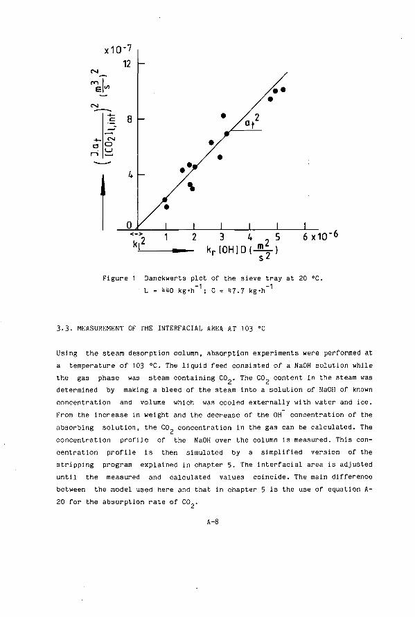
«VI

m I

<vi

cvi O

W

U ' 12

8

U

o ,

—

I l

•

/ •

I

A1

i i i 6 x10"

kr[0H]D m'

Figure 1 Danckwerts plot of the sieve tray at 20 °C. L = 140 kg'h"1; G = 1)7.7 kg-h"1

3-3. MEASUREMENT OF THE INTERFACIAL AREA AT 103 °C

Using the steam desorption column, absorption experiments were performed at a temperature of 103 °C. The liquid feed consisted of a NaOH solution while the gas phase was steam containing C0p. The CO, content in the steam was determined by making a bleed of the steam into a solution of NaOH of known concentration and volume which was cooled externally with water and ice. From the increase in weight and the decrease of the OH concentration of the absorbing solution, the C0? concentration in the gas can be calculated. The concentration profile of the NaOH over the column is measured. This con­centration profile is then simulated by a simplified version of the stripping program explained in chapter 5. The interfacial area is adjusted until the measured and calculated values coincide. The main difference between the model used here and that in chapter 5 is the use of equation A-20 for the absorption rate of CO..

The results of two experiments are shown in figure 2. These experiments differ slightly with respect to G, [OH ] and [CO ] . . It turns out that both experiments can be simulated very well with a value of He.. / a. equal

-i -2 ^ 2

to 235 atm«kg-mole This implies that any error in the Henry coeffi­cient directly influences the value of a . If He__ is taken to be equal to _1 t tu2 ' 135 atm-kg-mole as discussed above, we calculate the interfacial area at

2 -1 103 °C, a as = 0.6 m and a as 421) m .

OH" absorption profile — simulated • measured

4 6 8 10 - number of trays (-)

Figure 2 Concentration profile of hydroxide ions for CO absorption experiments in the tray column at 103 °C. L = H00 kg-h

I [OH ]. = 0.378 mol«kg •1 C02,in 3.141 -10~2 atm; G = 17.5 kg-h II [OH ] = 0.625 mol-kg ; P . = 5.08-10

11« U U 2 > ill -2 atm; G = 53.1 kg-h

A-9

3.1. MEASUREMENT OF THE GAS MASS TRANSFER COEFFICIENT AT 103 °C

With the available knowledge on the interfacial area and the liquid mass transfer coefficient, the gas phase mass transfer coefficient can be deter­mined from measurements on the desorption of a very soluble gas in water such as NH . Experiments on NH steam stripping was done in the desorption column. For the NH,/H?0 system, the simulation model can be based on equa­tions A-23 to A-21.

-mass transfer for a single tray

JNH3at " kolat( [NH3]l,b- [NH3]1 > (A"23)

with k , following from ol

k ,a. E.,kna. m.„, k a. ol t N i t NHj g t (A-23)

The enhancement factor, E„, was taken into account to express the influence N

of ionization on the desorption. For the enhancement factor holds

AN EN " AÏNHpi

(A"2,,)

where the A is the difference between bulk and interfacial concentration. The predicted concentration values are fitted to measured NH., concentrations giving the k a for NH . The ammonia desorption experiments are given in figure 3 a and b ( for low and high initial concentrations ). An excellent agreement is obtained with

-4 3 -1 -2 k ,a. equal to 2.4'10 nr-s , which finally yields a k value of 9-10

-T - 3 - 1 2 m-s when k is 1-10 m-s and a equals 0.6 m . The influence of the ionization is rather small: the value of the enhancement factor is 1.01 at the top and 1.06 at the bottom.

A-10

0.15

0.10

0.05

NH3 desorption profile

— simulated • measured

NH3 desorption profile

— simulated • measured

U 6 8 10 — number of trays (-)

i 6 8 10 — number of t rays ( - )

Figure 3 Concentration profi le of ammonia for desorption experiments in the tray column at 103 °C. L = 100 kg-h a) low concentration ; G = Ml.6 kg-h b) high concentration ; G = I t . t kg-h

3 . 5 . COMPARISON WITH LITERATURE

In the table 1 and 2 a l l r esu l t s from the l i t e r a t u r e correla t ions and ex­periments have been summarized. This has been done for two temperatures of 20 and 103 °C. In table 3 a l l physical parameters and average operating conditions used are given.

A - 1 1

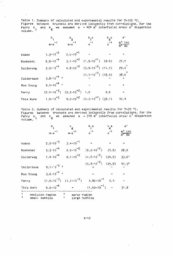
Table 1. Summary of calculated and experimental results for T=103 °C. Figures between brackets are derived indirectly from correlations. For the

volume. Perry k and k^ we assumed a = 424 m interfacial area/ m dispersion

k, k k, a k a a' 1 g 1 g -1 -1 -1 -1 m2 int

m-s m-s s s p - ^

Asano 1 .3• 10~2 5.5-10~1 - -

Nonhebel 6.9-10_lt 3-1-10~2 (1.9-10-1) (8-6) 27.7

Zuiderweg 2.0-10-14 4.8-10~2 (5.9-10-2) (14.1) 29.4

(7.7-10-2) (18.5) 38.6 Calderbank 3.8-10- 3 _ _ -

-4

Moo Young 9.4-10 *

Perry (2.4-10~3) (2.2-10~2) 1.0 9.5

This Work 1.0-10~3 9.0-10"2 (4.2-10~2) (38.1) 42.4 Table 2. Summary of calculated and experimental results for T=20 °C. Figures between brackets are derived indirectly from correlations. For the " '-, and k we assumed a = 318 m interfacial area/ m dispersion

1 g volume. k a

g -1 s

a '

m2 i n t m2 BA

k, k k a 1 g 1 -1 -1 -1

m-s m-s s Asano 5.2-10-3 3-4-10-1 - - -

Nonhebel 3-3-10_i4 2.0-10~2 (9.2-10~2) (5.6) 28.0

Zuiderweg 1.4-10-4 6.1-10-2 (4.7-10~2) (20.5) 33.6'

__ (5.9-10-2) (25.8) 42.32 Calderbank 9.1-10 3

-4 Moo Young 3.6-10 "

Perry (1.5-10~3) (1.7-10-2) 4.80-10-1 5.4 -4 -1

This Work 5.0-10 - (1.59-10 ) - 31.8 emulsion regime 2 spray regime small bubbles " large bubbles

A-12

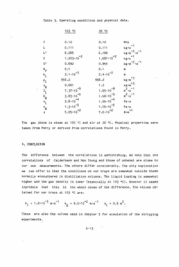
Table 3. Operating conditions and physical data.

103 °C 20 °C

P 0.12 L 0.111 L' 6.288 G 1.223-1o" G* 0.692 Hf 0.1 hl 2.1-10~2 P1 956.2 p_ 0.661 8 -9

01 7.37-10 D„ 3.83-10-5

•2

g r^ 2.8-10 ng 1.3-10-0 5.05-10

5 2

0.10 0.111 6.288 1.687-10-2 0.955 0.1 2.l)-10"2 )8.2 1.2 1.65-10-9 1 .58-10-5

-4 1.05-10 1 .78-10-5

7.0-10"2

MPa kg-s

-2 -1 kg-m -s kg-s

-2 -1 kg-m -s m m

-3 kg-m -3 kg-m

2 -1 m -s 2 -1 m -s Pa -s Pa-s N-m_1

The gas phase is steam at 103 °C and air at 20 °C. Physical properties were taken from Perry or derived from correlations found in Perry.

1. CONCLUSION

The difference between the correlations is ashtonishing. We note that the correlations of Calderbank and Moo Young and those of onhebel are close to our own measurements. The others differ considerably. The only explanation we can offer is that the conditions on our trays are somewhat outside those normally encountered in distillation columns. The liquid loading is somewhat higher and the'gas density is lower (especially at 103 °C). However it seems inprobale that this is the whole cause of the difference. The values ob­tained for our trays at 103 °C are:

k1 = 1.0-10-3 m-s~1 k = 9.0-10-2 m-s"1 a = 0.6 m2.

These are also the values used in chapter 5 for simulation of the stripping experiments.

A-13

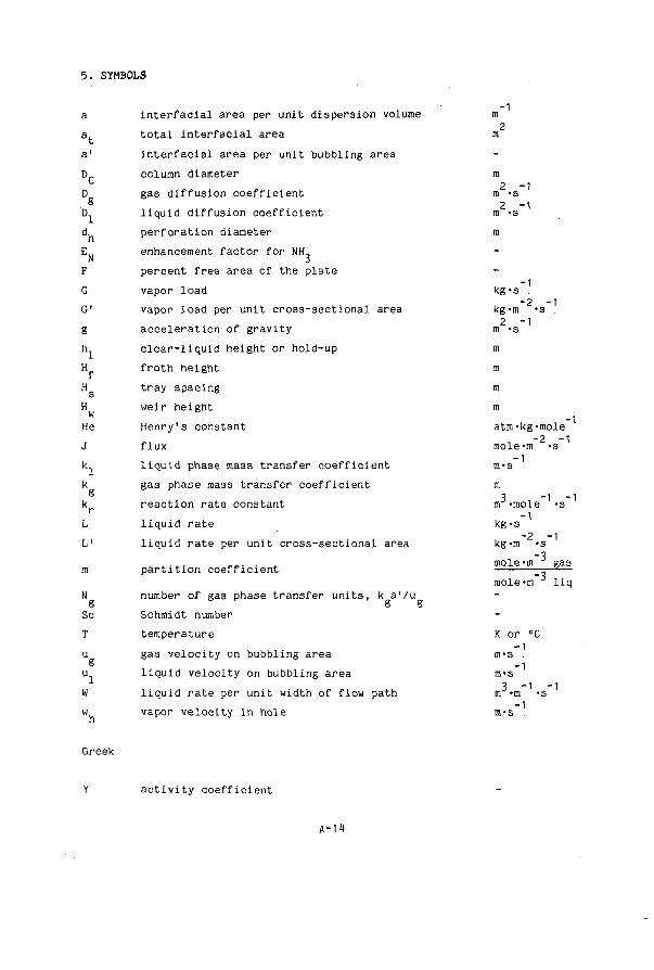
5. SYMBOLS

a interfacial area per unit dispersion volume m 2 a. total interfacial area m

a' interfacial area per unit bubbling area D- column diameter m

2 - 1 D gas diffusion coefficient m >s g

g

2 -1 D liquid diffusion coefficient m -s dh perforation diameter E„ enhancement factor for NH_, N 3 F percent free area of the plate G vapor load G' vapor load per unit cross-sectional area g acceleration of gravity h clear-liquid height or hold-up H froth height H tray spacing H weir height w He Henry's constant J flux k. liquid phase mass transfer coefficient k gas phase mass transfer coefficient k reaction rate constant L liquid rate L' liquid rate per unit cross-sectional area m partition coefficient

N number of gas phase transfer units, k a'/u g g g

Sc Schmidt number T temperature K or ° u gas velocity on bubbling area m-s .

kg-s kg-m 2 -m -s m m m m

-1 -2_ ■1

atm-kg-i mole ra-s m

■m I

m -mole kg-s kg-m mole mole

-1 -2_ •m •m

-1 u liquid velocity on bubbling area 3 - 1 W liquid rate per unit width of flow path m -m

w vapor velocity in hole m-s .

Greek

activity coefficient

A-14

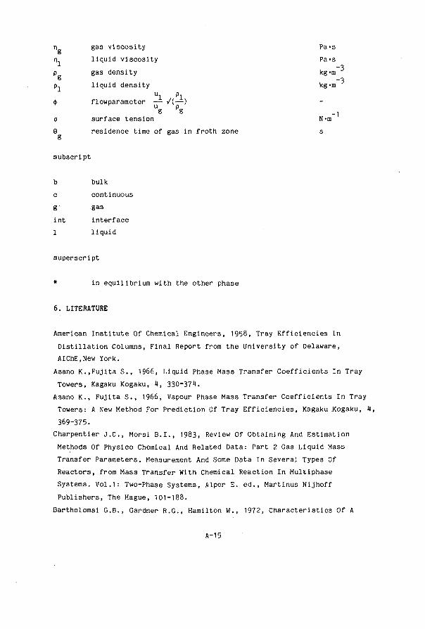
n gas viscosity n. liquid viscosity p gas density p liquid density

ul pl ij) flowparameter — /(—) Ug PS

o surface tension 0 residence time of gas in froth zone g

subscript

b bulk c continuous g' gas int interface

1 liquid

superscript

* in equilibrium with the other phase

6. LITERATURE American Institute Of Chemical Engineers, 1958, Tray Efficiencies In Distillation Columns, Final Report from the University of Delaware, AIChE.New York. Asano K.,Fujita S., 1966, Liquid Phase Mass Transfer Coefficients In Tray Towers, Kagaku Kogaku, 1, 330-371.

Asano K., Fujita S., 1966, Vapour Phase Mass Transfer Coefficients In Tray Towers: A New Method For Prediction Of Tray Efficiencies, Kagaku Kogaku, 1, 369-375.

Charpentier J.C., Morsi B.I., 1983, Review Of Obtaining And Estimation Methods Of Physico Chemical And Related Data: Part 2 Gas Liquid Mass Transfer Parameters. Measurement And Some Data In Several Types Of Reactors, from Mass Transfer With Chemical Reaction In Multiphase Systems. Vol.1: Two-Phase Systems, Alper E. ed., Martinus Nijhoff Publishers, The Hague, 101-188.

Bartholomai G.B., Gardner R.G., Hamilton W., 1972, Characteristics Of A

Pa-s Pa-s kg-m kg-m

N-m" s

A-15

Sieve Plate With Downcomer, Brit.Chem.Eng.& Proc.Tech.,17,48-50. Calderbank P.H., Moo-Young M.B., 1961, The Continuous Phase Heat And Mass Transfer Properties Of Dispersions, Chem.Eng.Sci., 16, 39-54. Coulson J.M., Richardson J.F., 1978, Chemical Engineering, Volume 2, Pergamon Press, London, 511.

Danckwerts P.V., 1975, Gas Liquid Reactions, Mc-Graw Hill, New York. Danckwerts P.V., Sharma M.M., 1966, The Absorption Of Carbon Dioxide Into Of Alkalis And Amines, The Chemical Engineer, CE244-CE280. Edwards T.J., Maurer G., Newman J., Prausnitz J.M., Vapor Liquid Equilibria In Multicomponent Aqueous Solutions Of Volatile Weak Electrolytes, 1978, AIChE J., 21,966-976. Nonhebel G., 1972, Gas Purification Processes For Air Pollution Control Butterworth & Co., London, 105-107. Pasiuk-Bronikowska W., 1969, Attempts To Determine The Liquid Film Coefficient For Physical Absorption, Chem.Eng.Sci., 24, 1139-1147. Perry R.H. , Green D.W., 1984, Chemical Engineers' Handbook, Sixth Ed., Mc Graw Hill New York, 18/5-18/16 Pinsent B.R.W., Pearson L., Roughton F.J.W., The Kinetics Of Combination Of Carbon Dioxide With Hydroxide Ions, 1956, Trans. Faraday Soc, 52, 1594-1598. Porter K.E., King M.B., Varshney K.C., 1966, Interfacial Areas And Liquid Film Mass Transfer Coefficient For A 3 FT Diameter Bubble Cap Plate Derived From Absorption Rates Of CO. Into Water and Caustic Soda, Trans.Instn.Chem.Engrs., 44, T274-T283. Treybal R.E, 1981, Mass Transfer Operations, Third Ed., Mc Graw-Hill, New York, 183. Zuiderweg F.J., 1982, Sieve Trays -A View Of The State Of The Art-, Chem.Eng.Sci., 37, 1441-1461.

A-16

APPENDIX 2

EXPERIENCE WITH AN OPTICAL PROBE FOR MEASURING BUBBLE SIZES AND VELOCITIES ON A SIEVE TRAY.

1. INTRODUCTION

As others have also experienced, we found the chemical methods for determin­ing mass transfer parameters time consuming and not very accurate. An alternative physical method has been developed by Calderbank and his co-workers (Burgess and Calderbank 1975a, 1975b; Calderbank and Pareira 1977; Calderbank 1978; Raper et al. 1978 and 1982. In these publications a physi­cal method is described which allows the determination of -bubble size and velocity distributions and -local gas porosities in sieve tray froths by "a press on a button". From these measured data it is possible to calcu­late (with some assumptions) k , k and a separately. The interfacial area is determined from the porosity and bubble size distribution, the mass transfer coefficients from the diffusion coefficients and a characteristic time, which is the bubble length divided by its velocity. Attempts were undertaken to develop a conductivity probe as described by Burgess et al.. The construction of the probe in combination with the production of step response signals turned out to be cumbersome. A far better system using optical probes has been developed by Frijlink. We were able to try out this system on our model tray.

2. PRINCIPLE

The bubble probe consists of a point gas liquid continuity detector sur­mounted by an array of three further detectors (see figure 1). Optical probes produce much sharper response curves than conductivity probes in a dispersion because they do not suffer from the disadvantage that the con­ducting liquid drains from the probe tip at a finite rate.

A-17

. /

2mm i

h X •

0.6mm

' Ibl 0.2mm

Figure 1. Lay out and the dimensions of the probe.

t/1

1 1

CM

-

h T2

a c

m (/) *3

«3

-* «/> u

/ 4 >

time Figure 2. Signals obtained from the passage of a bubble.

A-18

The optical probe can sense changes in refractive index at its extremity. Light is brought into the fibre and guided down to the extremity. If this in a medium of low refractive index (a gas) the light is reflected and detected. Otherwise it passes into the liquid. A typical signal for the passage of one bubble is given in figure 2. With the probe positioned vertically, the time for the leading surface to travel from detector 1 to the horizontal plane of detectors 2, 3 and 4 gives the bubble velocity.

2-10"3 (m) ... u = - t (1)

av

where t is the average of the times t„, t and tj,. This velocity gives the bubble central axis length:

1 = u-T1 (2)

where T is the time at which the bubble has passed detector 1 completely. The gas porosity can be calculated from the total time a probe is in the gas divided by the total time of the experiment:

£g " ( 3 ) Ï "1

Unfortunately the instrumentation feature to calculate the porosity was not yet avaible. The probe system accepts, within a certain tolerance, only those bubbles whose central axes coincide with the vertical probe axis. This acceptation is done by calculating the ratio's

t - t - i - — — f0r i = 2, 3 and 4 (4)

av

which should be smaller than a certain percentage. A furthur selection could be carried out upon the direction of the bubble velocity. For a (desired) vertical velocity the times T , T and Tü should be equal. This criterium was not used. All data are collected with an on-line computer so averages can be taken over large numbers of bubbles.

A-19

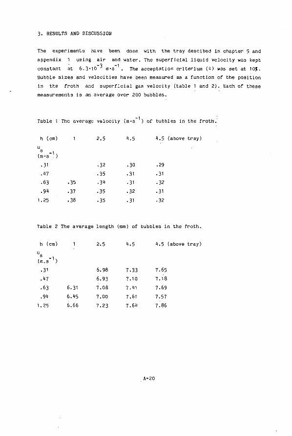
3. RESULTS AND DISCUSSION

The experiments have been done with the tray descibed in chapter 5 and appendix 1 using air and water. The superficial liquid velocity was kept

-3 -1 constant at 6.3*10 m*s . . The acceptation criterium (1) was set at 10%. Bubble sizes and velocities have been measured as a function of the position in the froth and superficial gas velocity (table 1 and 2). Each of these measurements is an average over 200 bubbles.

Table 1 The average velocity (m-s ) of bubbles in the froth.

h (cm)

u 3 - 1

(m-s . )

.31

.47

.63

.94

1.25

1

.35

.37

.38

2 . 5

• 32

. 35

• 3-t

.35

.35

1.5

.30

.31

.31

• 32

.31

1.5

.29

• 31

• 32

.31

.32

1.5 (above tray)

Table 2 The average length (mm) of bubbles in the froth.

1.5 (above tray) h (cm)

u

(m.s )

.31

.17

.63

. 91

1.25

6.

6.

6.

1

.31

.45

.66

2 .5

6.98

6 .93

7 .08

7 .00

7 .23

1.5

7 .33

7 .10

7 .41

7 .61

7 .64

1.5

7.65

7 .18

7 .69

7.57

7.86

A-20

The results show surprisingly little variation; they are all close to the average velocity of 0.33 m-s . and length of 7.3 mm. As discussed above the bed porosity could not measured by the instrument. The liquid porosity was calculated from the froth height and the clear liquid height, which was measured with a manometric technique, giving e, = 0.3 and 0.25 for the low and high gas velocities respectively. Due to bed expansion e decreases slightly with increasing gas velocity. The average local gas velocity can be calculated from

Ü=A- (5)

In all cases it exceeeds the bubble velocity. This rather surprizing result can be explained as follows. The gas flow is not uniformly distributed; a part f bypasses the bed through channels above the tray perforations. The velocity in the bed will then be:

u = - ^ (6)

With known values of u, u and e. we can calculate the bypass fraction. Results are presented in figure 3, together with similar results from Raper et al. (1978) and from Ashley and Haselden (1972). The latter data have been obtained after some manipulations with the data from their publication. The Ashley data indicate very large bypass fraction. The presence of bypass on our tray was also confirmed photographically. Photographs viewed fr'om verti­cally above the froth indicated large holes in the froth and in some cases it was possible to see down to the plate itself, which is remarkable through a froth depth of about 10 cm. The mass transfer coefficients and interfacial area are estimated with the familiar equations

k = 2-/(^) (7) and a = g (8)

With D = 2-10 and D = 2-10_5 m -s"1 , ü = 0.33 m-s"1 , 1= 7.3-10~3 m and e = 0.72 it follows that k1 = 3.«I• 10~ m-s"1, k = 3.i|-10~ m-s"1 and a = 590 m"1 . The transfer coefficients are in agreement with those known from the chemical method,

A-21

-1) -1 -2 -1 which gave k = 5'10 m-s and k «■ 4.5-10 m's . The specific area is a factor 1.8 higher ( a . = 318 m ). It is not surprising that mass trans-ehem fer coefficients and/or interfacial area are higher for the physical method. In the chemical method the effect of the gas bypass is always neglected. This means that the c value in the rate equations is misinterpreted: the value used is too low. In reality the liquid can only reach equilibrium with the gas fraction passing through the bed. When measured mass transfer rates are interpreted with an incorrect driving force term (too high), the propor­tionality constant k-a derived from the rate equation is also misinterpreted (too low). The bypassing model also allows an estimate to be made of the Murphree tray efficiency. From a mass balance can be shown that for the tray efficiency E holds mv

Emv * f-Emv,by + ( W ) 'Wub (9)'

With the assumptions E . = 0 and equilibrium for the small bubbles in the mv.byp bed expressed as E . = 1 it follows that K mv.bub

E = 1 - f (10) mv

We have measured efficiencies for the stripping of ammonia at 103 °C at similar trays in our steam desorption column. Many experiments have been

-1 -3 carried out around F = 0.9 m-s /(kg-m ). This should have yielded a bypass of around of about 50% and also a tray efficiency of this value. In reality we found efficiencies of 80 to 85% indicating that the bypass assumptions used are too simple.

A-22

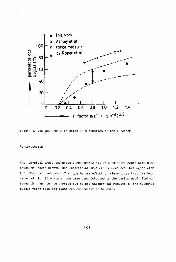
(/I a 0 1 _

a •*-c <u l_> 1_ 01 GL .

• this work x Ashley et al

^ 00 _ ^ range measured by Raper et al.

£ 80 : t 40

20

0

/ / /

/ / / '

• >

I I''* I _L 0 0.2 0.4 0.6 0.8 1.0 1.2 1.4

» — F factor m.s"1 ( kg.m"3 ) o s

Figure 3. The gas bypass fraction as a function of the F factor.

1. CONCLUSION

The physical probe technique looks promising. In a relative short time mass transfer coefficients and interfacial area can be measured that agree with the chemical methods. The gas bypass effect on sieve trays that has been reported in literature has also been detected by the system used. Further research has to be carried out to see whether the results of the measured bubble velocities and diameters can really be trusted.

A-23

5. SYMBOLS

E Murphree efficiency mv K

f bypass fraction k mass transfer coefficient 1 length t,T time u velocity

Greek

e porosity (-)

6. LITERATURE

Ashley M.J., Haselden G.G., 1972, Effectiveness of Vapour-Liquid Contacting On A Sieve Plate, Trans. Instn. Chem. Engrs., 50, 119-124. Burgess J.M., Calderbank P.H., 1975, The Measurement Of Bubble Parameters In Two Phase Dispersions -I The Development Of An Improved Probe Technique, Chem.Eng.Sci., 30, 743-750. Burgess J.M., Calderbank P.H., 1975, The Measurement Of Bubble Parameters In Two Phase Dispersions -II The Structure Of Sieve Tray Froths, Chem.Eng.Sci. 30, 1107-1121.

Calderbank P.H., 1978, Limitations Of Burgess-Calderbank Probe Technique For Characterization Of Gas Liquid Dispersions On Sieve Trays, Chem.Eng.Sci., 33, 1^07.

Calderbank P.H., Pereira J, 1977, The Prediction Of Distillation Plate Efficiencies From Froth Properties, Chem.Eng.Sci., 32, 1127-1133. Frijlink J.J., Ph.D. Thesis in preparation, Delft University Of Technology Raper J.A, Dixon D.C., Fell C.J.D., Burgess J.M., 1978, Limitations Of Burgess-Calderbank Probe Technique For Characterization Of Gas Liquid Dispersions On Sieve Trays, Chem.Eng.Sci, 33, 1105-1406. Raper J.A., Kearney M.S., Burgess J.M., Fell CD., 1982, The Sructure Of Industrial Sieve Tray Froths, Chem.Eng.Sci., 37, 501-506.

(-) (-)

-1 m*s m s

-1 m-s

A-24

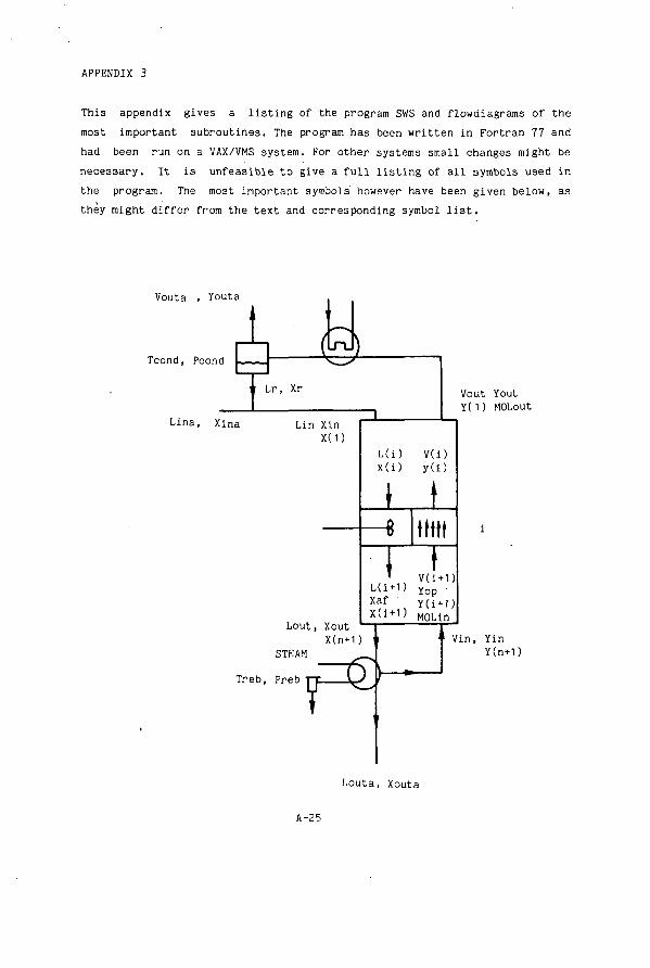
APPENDIX 3

This appendix gives a listing of the program SWS and flowdiagrams of the most important subroutines. The program has been written in Fortran 77 and had been run on a VAX/VMS system. For other systems small changes might be necessary. It is unfeasible to give a full listing of all symbols used in the program. The most important symbols however have been given below, as they might differ from the text and corresponding symbol list.

Vouta , Youta

Tcond, Pcond «. © |' Lr, Xr

Lina, Xir Lin Xin X(1)

L(i+1)

L(i) V(i) x(i) y(i)

' , V(i+

Vout Yout Y( 1) MOLout

1) Yop

Lout, Xout X(n+1) "

Xaf Y ( i + 1 ) x<1+1> MOLin

STEAM

Treb, Preb T € » -1 Vin, Yin

Y(n+1)

Louta, Xouta

A-25

MAIN PROGRAM

| INITIALIZATION

| READ INPUT FILE|

WRITE INPUT DATA TO OUTPUT FILE

CALC TEMP AND PRESS PROFILE

CALC MEAN STRIPPING FACTOR

label 70-150

label 160-170

label 180

I CALC NEW EST

FOR Xou ta

(SUBR ADJUST)

ESTIMATE Xouta WITH KREMSER EQ

( I F S, < 1.0)

DO COLUMN CALCULATION

(SUBR COLUMN)

WRITE RESULTS TO OUTPUT FILE l a b e l 190-770

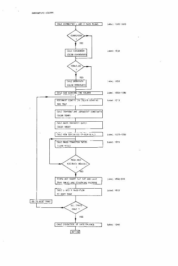
SUBBOUTINE COLUMN

| CALC COBBECTED L AND V MASS FLOWS ~| label 1600-161

CALC CONDENSOB (SUBR CONDENSOR]

CALC REBOILER (SUBR REBOILEB)

| CALC GAS LEAVING THE COLUMN

ESTIMATE CONC'S IN LIQUID LEAVING THE TSAY

CALC TEMPERATURE DEPENDENT CONSTANTS (SUBR TEMP)

CALC MASS TRANSFER RATES (SUBR MBSO)

CALC NEW ESTIMATES («-DIM N.R.)

CALC MASS TRANSFER RATES I.SL'BR MBSO)

STOBE ACT COEFF (AT 1ST AND LAST TRAY ONLY) AND STBIPPING FACTORS

CALC L AND V MA3S-FL0W AT NEXT TRAY

GO TO NEXT TRAY

CALC DEVIATION OF MASS BALANCE

label 1630

label 1660-1680

label 1710

label 1720-1860

label 1870

label 1880-900

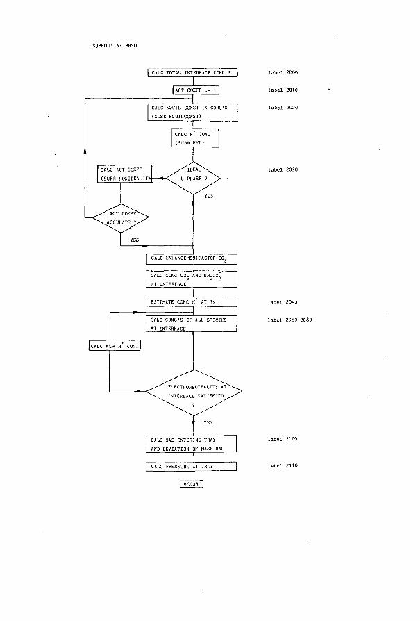
SUBROUTINE HBSO

CALC TOTAL INTERFACE CONC'S

I ACT COEFF : - 1 I

I CALC EQUIL CONST IN CONC'S (SUBR EQUILCONST)

CALC H CONC (SUBR HYD)

CALC ACT COEFF (SUBR «ONIDEALITY

CALC ENHANCEMENTFACTOR CO,

AT INTERFACE

CALC CONC'S OF ALL SPECIES AT INTERFACE

CALC NEW H CONC

CALC CAS ENTERING TRAY AND DEVIATION OF MASS BAL

I RETURiil

ESTIMATE CONC H AT INT

CALC PRESSURE AT TRAY

l a b e l 2010

l a b e l 2030

l a b e l 2010

l a b e l 2050-2080

SUBROUTINE CONDENSOR

INITIALIZATION

GIVE WARNING

CALC TEMP DEPENDENT CONSTANTS

(SUBR EQUILIBRIUM)

CALC COMP OF GAS LEAVING COND

CALC COMP OF. Lr IN EQ WITH Vouta

3 l a b e l 810-830

"1 l a b e l 810-850

CALC LIQUID ENTERING COLUMN

(FEED ♦ REFLUX)

CALC GAS LEAVING COLUMN

(GAS LEAVING CONDENSOR * REFLUX)

l a b e l 880-900

SUBROUTINE REBOILER

INITIALIZATION

CALC TEMP DEPENDENT CONSTANTS

(SUBR EQUILIBRIUM)

CALC CONC'S FREE COMP'S IN LIQUID

LEAVING REBOILER

GIVE WARNINC * - < T REBOILER PRESSURE

i YES

CALC LIQUID LEAVING THE COLUMN

(LIQ LEAVING REB.-GAS ENTERING COL.)

l a b e l 1100-1120

CALC COMP OF GAS LEAVING REBOILER ] l a b e l 1130-UKO

[Hinf

DUAO:[USERS.H00GENDO0]PUBL.MEM; 1

Input file: (this file contains all input data required to run the program. it must be available to the program with the name: INPUT.DAT)

no. of trays: Lin: steam: id: con:reb:gasin: 11 0.10000D+03 0.<*5500D+02NO NO NO NO

Xin: NH3 ' H2S ' C02 phenol water 0.17t90D+00 0.09115D+00 0.00560D+00 0.00336D+00 O.OOOOOD+00

Xout:NH3 H2S C02 phenol water 0.00000D+00 O.OOOOOD+00 O.OOOOOD+00 0.00000D+00 0.00000D+00 temp.:top ' bottom ' cond. reb. pres.:top bottom 0.37400D+03 0.37600D+03 0.37300D+03 0.37600D+03 0.10500D+01 0.11000D+01

pres.:cond. reb. kl: kg: a: 0.10000D+01 0.10000D+01 0.10000D-02 0.90000D-01 0.60000D+00 This line must'contain an identifier, which is printed in the output file.

(note: the identifier must have a length of 71 characters.)

Program: (the program reads input data from the file INPUT.DAT and writes output data to the file RESULT.LIS)

e******************************************************************************* C C SIMULATION PROGRAM FOR SOUR WATER STRIPPING. C (simulation is done for NH3, H2S, C02 and phenol. C components are indicated as no. 1,2,3 and 4 respectively.) C program written by: C P.J.M. ESSENS C T.U. DELFT C JANUARI 1986 C

C declaration arrays: IMPLICIT DOUBLE PRECISION (A-H.K.O-Z) DIMENSION NIND0 2) .NREGEL1 (18) ,NREGEL2( 18) ,NREGEL3( 18) ,

1 NREGELM18),NREGEL5(18),NCOMP(12),XOUTA(5),PRO(!0, 1 HULP(t),KSIGEM(H),NIDENT(l8),NAAM(5),REKGEM(M)

DOUBLE PRECISION L.LIQU,LIN,LINA,LOUT,L0UTA.LR,MOLEN, 1 MOLOUT(5),MOLW,M(lJ)

LOGICAL NONIDEAL,CONDENS,REB0IL,FIRST,STOP,WARNING,PRESWARN, 1 GASIN

COMMON /CON/XINA(5),XIN(5) ,TCOND,PRESCON,OPENST,LIN,LINA, 1 LR,YOUT(5),YOUTA(5),XR(5),YOUT2(5),VOUT,VOUTA,PRESWARN

COMMON /REB/YIN(5),LOUT,TREB,PRESREB,REBST,LOUTA,CREB,VIN, 1 WARNING

COMMON /COL/NMAX,Y(5,5D ,FAO) ,L,M0L0UT,DELTAM(3) ,STOOM COMMON /EQ/HECM) COMMON /GAM/BETA0(11,11),BETA1(11,11),CHARGE(13) COMMON /MBSO/DC02,KRBICAR,KRCARB,KL,KLA,KGA,FLUX(H) COMMON /HEN/HEN(10,M,RHOL,DHC COMMON /TEMP/TTOP,TBOT,T(50) COMMON /P/PRES(50) COMMON /X/X(5,52),XOUT(5) COMMON /ID/STOP,NONIDEAL,CONDENS,REBOIL,GASIN COMMON /V/V.C COMMON /GAMUIT/GAMUITCJ,12) COMMON /ACT/WACT,ACT(4) COMMON /STREAM/LIQU(51),VAP0(51),STRIPCJ,50),RHO(50) COMMON /H/H(50),DRUK(50)

DUAO:[USERS.HOOGENDOO]PUBL.MEM; 2

OPEN (UNIT-1,FILE-'RESULT.LIS',STATUS='NEW') OPEN (UNIT=2,FILE='INPUT.DAT',STATUS='0LD')

C initialization arrays: C (first interaction parameter according to Maurer)

DATA BETAO/ .00669, .0117, -.01135, -.0816, .068, 1 .015, .0119, -.0201, -.0119,' .032,

1 .0117, .0, .00166, -.0135, -.062, 1 .0, .06, .0839, .0638, -.021,

1 -.01135, .00166, -.09539, .0, .0, 1 .033, .05916, -.0712, .0, .053,

1 -.0816, -.0135, .0, .0, .0, 1 .071, .0, -.037, .0, .0,

1 .068, -.062, .0, .0, .0, 1 .086, .0, .077, .0, .0,

1 .0, .0505, .017, .0, .0, 1 .198, .0, -.032, .0, .0,

1 .015, .0, .033, .071, .086, 1 .0, .208, .017, ■ .191, .127,

1 .0119, .06, .05916, .0, .0, 1 .208, ' .0, .0173, .0, .0,

1 -.0201, .0839, -.0712, -.037, .077, 1 .017, .0173, -.01688, .0, .0,

1 -.0119, .0638, .0, .0, .0, 1 .191, .0, .0, .0, .0,

1 .032, -.021, .053, .0, .0, 1 .127, .0, .0, .0, .0/

C . . . C (second interaction parameter according to Maurer)

DATA BETA1/ .0, -.02, .0, .1829, .0, 1 .0, .0, .0, .106, .0, 1 -.02, .0, .0, -.1151, -.1717, 1 .0, .2016, .0, .2132, -.0163,

1 .0, .0, .0, .0, .0, 1 .0, .0, .0, .0, .0,

1 .1829, -.1151, .0, .0, .0, 1 .2353,' .0, .0, .0, .0,

1 .0, -.1717, .0, .0, .0, 1 .2812, .0, .0, .0, .0,

1 .0, .1725, .0, .0, .0, 1 .6239, .0, .0, .0, .0,

1 .0, .0, .0, .2353, .2812, 1 .0, .6515, .0, .6116, .1066,

1 .0, .2016, .0, .0, .0, 1 .6515, .0, .0, .0, .0,

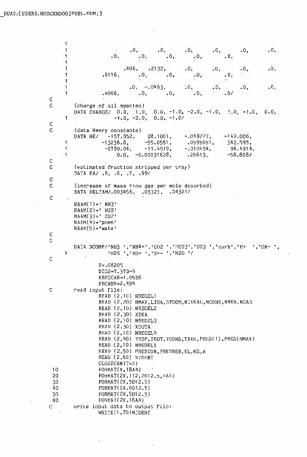
DUA0:[USERS.HOOGENDOO]PUBL.MEM;3

. 0 , . 0 , . 0 , . 0 , . 0 , . 0 , . 0 , . 0 ,

. 1 0 6 , . 2 1 3 2 , .6116, . 0 , . 0 ,

. 0 , . 0 , . 0 , . 0 ,

.4066, . 0 , - . 0 4 6 3 ,

. 0 , . 0 , . 0 , . 0 ,

. 0 ,

. 0 ,

. 0 ,

. 0 ,

. 0 , . 0 / c c

c c

c c c c c

c c c

c

10 20 30 40 50 60 C

(charge of all species) DATA CHARGE/ 0.0, 1.0, 0.0, -1.0, -2.0, -1.0, 1.0, -1.0

-1.0, -2.0, 0.0, -1.0/

(data Henry constants) DATA HE/ -157.552, 28.1001, -.049227, -149.006,

-13236.8, -55.0551, .0595651, 342.595, -6789.04, -11.4519, -.010454, 94.4914,

0.0, -0.00031628, .26613, -58.808/

(estimated fraction stripped per tray) DATA FA/ .9, .6, .7, .99/

(increase of mass flow gas per mole desorbed) DATA DELTAM/.003456, .03321, .04321/

NAAM(1)=' NH3' NAAM(2)=' H2S' NAAM(3)=' C02' NAAM(4)='phen' NAAM(5)='wate'

DATA NC0MP/'NH3 ','NH4+','C02 ','HC03','C03 ','carb','H+ ' 'H2S ','HS- ','S-- ',*H20 '/

R=.08205 DC02=7.37D-9 KRBICAR=1.05D6 KRCARB=2.4D4

read input file: ' READ (2,10) NREGEL1 READ (2,20) NMAX,LINA,STOOM,NIDEAL,NCOND.NREB,NGAS READ (2,10) NREGEL2 READ (2,30) XINA READ (2,10) NREGEL3 READ (2,30) XOUTA READ (2,10) NREGEL4 READ (2,40) TT0P,TB0T,TC0ND,TREB,PRES(1).PRES(NMAX) READ (2,10) NREGEL5 READ (2,50) PRESCON,PRESREB,KL,KG,A READ (2,60) NIDENT CL0SE(UNIT=2) F0RMAT(X,18A4) F0RMAT(2X,I12,2D12.5,4A4) FORMAT(2X.5D1 2.5) F0RMAT(2X,6D12.5) FORMAT(2X.5D1 2.5) F0RMAT(2X,18A4)

write input data to output file: WRITEO ,70)NIDENT

0.0,

' O H -

DUAO:[USERS.HOOGENDOO]PUBL.MEM;1

70

95

115

80

90 100 110 120 130

110

150

F0RMATC1 ',//,5X,l8Al,//) WRITEd,80)NMAX,NIDEAL,NCOND,NREB,SNGLUINA/3600.0),

SNGL(LINA),SNCL(STOOM/3600.0),SNGL(STOOM) IF (NGAS .EQ. 'YES') THEN WRITEd ,90) GASIN=.TRUE. GO TO 95 ENDIF

WRITEd ,100) GASIN=wFALSE. WRITEd ,110) DO 115 1 = 1 ,1 WRITE(1,120)NAAM(I),SNGL(XINA(I)),SNGL(XOUTA(I)) CONTINUE

WRITEd,130)SNGL(TTOP-273.0),SNGL(TTOP),SNGL(TBOT-273.0),SNGL(TBOT! SNGL(TCOND-273.0).SNGL(TCOND),SNGL(TREB-273.0).SNGL(TREB)

WRITE(1,1tO)SNGL(PRES(1)),SNGL(PRES(NMAX)).SNGL(PRESCON), SNGL(PRESREB)

WRITEd ,150)SNGL(KL),SNGL(A),SNGL(KG) FORMAT(5X,'Number of Trays:',1OX,12,//5X,'Ideal liquid'

' phase:',8x,A3,/,5X,'Condensor:',16X,A3,/,5X, 'Reboiler:'17X,A3,//,5X'Lin:',12X,F8.5,' Kg/s or ', F10.3.' Kg/hr',/,5X,'Steam:'.10X.F8.5,' Kg/s or ', F10.3,' Kg/hr')

F0RMAT(8X,'(Steam = amount of gas entering the column)',//) F0RMAT(8X,'(Steam = amount of gas leaving the column)',//) F0RMAT(5X,'Component: Xin: Xout:') F0RMAT(7X,A5,5X,F8.5,6X,F8.5,' mol/kg') F0RMAT(/,5X,'Top temperature:',8X,F6.2,' C or ',F6.2,' K',/,

5X,'Bottom temperature:•,5X,F6.2,' C or ',F6.2,' K',/, 5X,'Condensor temperature:',2X,F6.2,' C or ',F6.2,' K',/, 5X,'Reboiler temperature:',3X.F6.2,' C or ',F6.2,' K',/)

F0RMAT(5X,'Top pres.:',7X,F8.t,' atm.',/,5X ,'Bottom pres.-.',1X, F8.lt.' atm. ' ,/,5X,'Condensor pres. : ' ,X , F8. 5X,'Reboiler pres.:',2X,F8.H,' atm.',/)

F0RMAT(5X,'K1:',2X,E11 .6,' m/s',5X,'A:',3X,E1 1.6, 5X,'Kg:',2X,E11.6,' m/s',/)

m2

atm. ' ,/,

,/,

initialization constants: KLA=KL*A KGA=KG*A LINA=LINA/3600.0 WARNING=.FALSE. PRESWARN=.FALSE. ST0P=.FALSE. N0NIDEAL=.FALSE. IF ((NIDEAL .EQ. 'NO') .OR. (NIDEAL .EQ. 'no'))

NONIDEAL=.TRUE. C0NDENS=.FALSE. IF ((NC0ND .EQ. 'YES') .OR. (NC0ND .EQ. 'yes')) CONDENS».TRUE. REBST=0.0 OPENST=STOOM/3600.0 REBOIL=.FALSE. IF ((NREB .EQ. ' Y E S ' ) .OR. (NREB .EQ. ' y e s ' ) ) THEN

REBOIL=.TRUE. OPENST=0.0 REBST=STOOM/3600.0 ENDIF

WACT=1 .0 DO 160 1 = 1 , 1

A C T ( I ) = 1 . 0

DUA0:[USERS.H00GENDOO]PUBL.MEM;5

160 CONTINUE C calculate temp, and pres. profile:

DO 170 N-1,NMAX PRES(N)=PRES(1)+DBLE(N-1)*(PRES(NMAX)-PRES(1))/DBLE(NMAX-1) T(N)=TT0P+(TB0T-TT0P)*DBLE(N-1)/DBLE(NMAX-1)

170 CONTINUE STOOM=STOOM/3600.0 V=ST00M C=PRES(1)/(V/.018) TGEM=(TTOP +TB0T)/2.0

C Kremser equation to estimate Xout: CALL EQUILIBRIUM(TGEM) RH0G=.018*PRES(1)/(.001*R*TGEM) DO 180 1=1,1 S=M(l)*RHOL*V/(RHOG*LINA) IF (S .LT. 1.0) THEN BEREKEND=(1.0-S)*XINA(I) IF (BEREKEND .GT. XOUTA(D) X0UTA( I)=BEREKEND ENDIF

180 CONTINUE C calculate column:

CALL TRAYCOLUMN(XOUTA,XIN,NMAX,NTEL) C if error in calculations then stop (no output):

IF (STOP) GO TO 770 WRITEO ,190)NTEL

190 F0RMAT(/,5X,'Required accuracy reached in ',I2,' iterations.') c . C output activity coefficients (optional):

IF (.NOT. NONIDEAL) GO TO 290 IF (XIN(1) .LT. 1.0E-6) THEN DO 200 1=1,1 GAMUIT(I,1)=.0 GAMUIT(I,2)=.0 GAMUIT(I,6)=.0

200 CONTINUE ENDIF

IF (XIN(2) .LT. 1.0E-6) THEN DO 210 1=1 ,1 GAMUIT(I,9)=.0 GAMUIT(I,10)=.0 GAMUIT(I,11)=.0

210 CONTINUE ENDIF

IF (XIN(3) .LT. 1.0E-6) THEN DO 220 1=1,1 DO 230 MM=3,6 GAMUIT(I,MM)=.0

230 CONTINUE 220 CONTINUE

ENDIF WRITEO ,210)NMAX

210 F0RMAT('1',//,5X,'Activity coefficients:',///,5X, 1 'Comp.: Tray 1: Tray ',I2,': Condensor: ' , 1 ' Reboiler:')

DO 250 1=1 ,12 WRITEO,260)NC0MP(I),SNGL(GAMUIT(1,I)),SNGL(GAMUIT(2,I)),

1 SNGL(GAMUIT(3,I)),SNGL(GAMUIT(1,D) 250 CONTINUE 260 FORMAT(6x,Al,1(2X,F10.7))

WRITEO ,270) WRITEO, 280)

DUAO:[USERS.HOOGENDOO]PUBL.MEM; 6

270 F0RMAT(/,5X,'Activity of water is defined as:', 1 ' Waet = gamma(H20) * molfr(H2o)')

280 FORMAT(/,5X,'(act .coeff.= 0.0 if component is not present in ', 1 'the feed or if',/,5X,'cond. and/or reb. is used.)')

C C output condensor (optional): 290 IF (.NOT. CONDENS) GO TO 380

WRITEd ,300)PRESCON,(TCOND-273) 300 FORMAT('1',//,5X,'Column with condensor and reflux:•,//,5X,

1 'Condensor pres.=',6X,F10.5,' atm.',/,5X, 1 'Condensor temperature=',F10.5,' C',/)

IF (PRESWARN) WRITE(1,310) 310 F0RMAT(//5X, ' ' ,

1 ' —'/5X,'| estimated pres. too low; Pcond=1.25*P(H20)' 1 ,' used | * /,5X, • ' , _. .//)

WRITEd ,320)LINA,LR,LIN 320 F0RMATU8X,' column',/,

1 18X,' feed: reflux: feed:',/, 1 5X,1 amount: ',3(2X,F10.6),' kg/s')

DO 330 1=1,H WRITEd, 3t0)NAAM(I),XINA(I),XR(I),XIN(I)

330 CONTINUE 310 F0RMAT(8X,A1,5X,3(F10.6,2X),' mol/kg H20')

WRITEd,350)V0UT,V0UTA 350 F0RMAT(//,18X,' gas lea- gas lea-*,/,

1 17X,'ving column: ving cond. : ',/,5X, 1 • amount: ',2(F10.6,2X),' kg/s')

DO 360 1=1,5 WRITEd ,370)NAAM(I),YOUT2(I),YOUTA(I)

360 CONTINUE 370 FORMAT(8X,AlJ,5X,2(F10.6,2X),' atm.')

C C output reboiler (optional): 380 IF (.NOT. REB0IL) GO TO 170

WRITE(1,390)SNGL(PRESREB),SNGL(TREB-273) 390 F0RMAT('1 ',//,5X,'column with reboiler :',//,5X,'reboiler pres. = '

1 ,6X,F10.5,/,5X,'reboiler temperature=',F10.5,/) IF (WARNING) WRITEd ,400)

1400 F0RMAT(5X 'ft******»»**********************»******************' , 1 /,5X,'* warning: estimated reboiler pres. is', 1 ' incorrect *' / 5X '************************' 1 i************»*»***********t //)

WRITEd ,410)SNGL(L0UT) .SNGL(LOUTA) 410 F0RMAT(18X,'liquid lea- liquid lea-',/,

1 17X,'ving column: ving rebo.:',/,7X, 1 'amount: ' ,2(F10.6,3X),' kg/s')

DO 1420 1 = 1 ,5 WRITE(1,l430)NAAM(I),SNGL(XOUT(I)),SNGL(XOUTA(I))

1420 CONTINUE 130 FORMAT(8X,AH,5X,2(F10.6,3X),' mol/kg')

WRITEd ,l4t0)SNGL(V) HHO F0RMAT(//,18X,'gas entering:',/,7X,'amount: ',

1 F10.6.' kg/s') DO 150 1=1,5

WRITEd ,160)NAAM(I),SNGL(YIN(I)) i»50 CONTINUE 460 FORMAT(8X,Al4,5X,F10.6, * atm.')

C output column pressure: WRITEd ,600)

600 F0RMAT('1 ',//,5X,'column pressure and mass flows:',//,

7 8-SEP-1986 16:31

input gas',/, pres . : flow:

calculated

pres. : './)

difference

> 51',

1 5X.' 1 ' liquid -1 5X,' tray: 1 ■ flow:

DO 610 1=1,NMAX MISDRUK='no' IF(DABS((PRES(I)-DRUK(I))/DRUK(I)) .GT. 0.05) MISDRUK='yes' WRITEO,620)I,PRES(I),DRUK(I),MISDRUK,LIQU(I),VAPO(I)

610 CONTINUE 620 F0RMAT( 8X , 12 , 7X , F7 . 4, 6X , F7. 4 , 8X , A3 , 3X , F1 0. 7 , 2X , F1 0 .7 )

WRITEC1,630) 630 F0RMAT(//,5X,'stripping factors: ' ,/,5X, ' tray: NH3: '

1 'H2S: C02: phenol: rhogas:') DO 640 1=1,NMAX

WRITE(1,650)I,STRIP(1,I),STRIP(2,I),STRIP(3,I),STRIP(1,I), 1 RH0(I)

610 CONTINUE 650 F0RMAT( 8X, 12, 3X, 4( F9.4, 2X), 2X , F8.6)

C output concentration profiles: WRITEO ,660)

660 F0RMATC1 V.5X,' tray: X(NH3): X(H2S): ', 1 'X(C02): X(phenol): pH:',/)

WRITEC1 ,670) XO,1),X(2,1),X(3,D,X(4,1) 670 F0RMAT(7X,'feed',2X,4(F12.6,X),' raol/kg')

DO 680 N=2,(NMAX+1) WRITE(1,690)(N-1),X(1,N),X(2>N),X(3,N),X(1,N),-DLOG10CH(N-1))

680 CONTINUE 690 FORMAT(8x,I2,3X,4(F12.6,X),' mol/kg',3X,F5.2)

WRITEO,700) 700 F0RMAT(/,5X,' tray: Y(NH3): Y(H2S): ',

1 'Y(C02): Y(phenol):',/) DO 710 N=1 ,(NMAX+1) WRITEO ,720) (N-1),YO,N),Y(2,N),Y(3,N),Y(4,N)

710 CONTINUE 720 F0RMAT(8X,I2,3X,1(F12.6,X),' atra.')

WRITEO ,730) 730 F0RMAT(//,5X,'Percentage stripped:',/)

DO 740 1=1,4 PRO(I)=0.0 IF (X(I,1) .LT. 1.0E-6) GO TO 750 PR0(I)=100.0*(1.0-LOUTA*XOUTA(I)/(LINA*XINA(I)))

750 WRITEO ,760)NAAM(I) ,SNGL{ PRO(I) ) 710 CONTINUE 760 FORMAT(7X,A4,1X,F6.2,' I')

C C graphical output concentration profiles:

CALL GRAF(NMAX) 770 CL0SE(UNIT=1)

STOP END

C**xxx*xxx*xxxx*xx**x»*xxxxxxxx*x*xxxxx*x»x*x*xxx*xx*xx**xxxxxxxxxxxx**xxxxxxxx C Function dett; calculates value of a 4*4 matrix.

DOUBLE PRECISION FUNCTION DET4(A,B.C,D) DOUBLE PRECISION HULP,A(4),B(4),C(4),D(4) HULP=AO)*(B(2)*(C(3)*D(4)-C(4)*D(3))-B(3)*(C(2)*D(4)-

1 C(4)*D(2))+B(4)*(C(2)*D(3)-C(3)*D(2))) HULP=HULP-A(2)*(BO)*(C(3)*D(4)-C(4)*D(3))-B(3)*(CO)*D(4)-

1 C(4)xD0))+B(4)*(CO)*D(3)-C(3)*DO))) HULP=HULP+A(3)*(B(1)*(C(2)*D(4)-C(4)*D(2))-B(2)*(C(1)*D(4)-

1 C(1)*D(1))+B(it)*(C(1)»D(2)-C(2)*D(1))) DET4=HULP-A(4)*(BO)*(C(2)*D(3)-C(3)*D(2))-B(2)*(c(1)*D(3)-

DUA0:[USERS.HOOGENDOO]PUBL.MEM;8

1 C(3)*D(1))+B(3)*(C(1)*D(2)-C(2)*D(1))) RETURN END

C***********************»*****x****************************«**************x**x** C Subroutine condensor; calculates condenser if present.

SUBROUTINE CONDENSOR(XOUTA) IMPLICIT DOUBLE PRECISION (A-H.K.O-Z) DOUBLE PRECISION ION,LIN,LINA,LOUT,LOUTA,L,LR,M(«).MOLFRACTIE,

1 MOLOUT(5),MOLEN,MOLW,MOLM DIMENSION GAMMA(11),P(5),XOUTA(5) LOGICAL ACTIVITY,NONIDEAL,CONDENS,REBOIL,STOP,PRESWARN COMMON /CON/XINA(5),XIN(5),TCOND,PRESCON.OPENST,LIN,LINA,

1 LR,YOUT(5),YOUTA(5),XR(5),YOUT2(5),VOUT,VOUTA,PRESWARN COMMON /REB/YIN(5),LOUT,TREB,PRESREB,REBST,LOUTA,CREB,VIN COMMON /X/X(5,52),XOUT(5) COMMON /COL/NMAX,Y(5,51),FA(lJ),L,MOLOUT COMMON /XRFREE/XRFREE(5) COMMON /K/KW,KN,KS1,KS2,KC1,KC2,KC3,KF COMMON /HEN/HEN(4),M,RHOL,DHC COMMON /ID/STOP,NONIDEAL,CONDENS,REBOIL COMMON /V/V.C COMMON /GAMUIT/GAMUITCM2) COMMON /P/PRES(50) COMMON /ACT/WACT,ACT(4)

C initialization: CCOND=25.0 NTEL=0

C calculate equilibrium pressure of water: PH20=1.315786E-3*(10**(8.07131-1730.63/(TCOND-39.574)) )

C check for impossible condensor pressure: IF (PRESCON .LT. PH20) THEN PRESWARN».TRUE. PRESC0N=1.25*PH20 ENDIF

C calculate temp, dependent constants: CALL EQUILIBRIUM(TCOND)

C initialization: Y0UTA(5)=PH20 VOUTA=0.0 DO 800 1=1 ,13 GAMMA(I)=1.0

800 CONTINUE ION-1 .0 WACT=1 .0

C start equilibrium calculation (iterative): 810 NTEL=NTEL+1 820 VOLD=VOUTA

L0UTA=LINA+0PENST-VOUTA MOLEN=LINA*(XINA(1)+XINA(2)+XINA(3)+XINA(<J))-

1 LOUTA*(XOUTA(1)+XOUTA(2)+XOUTA(3)+XOUTAO)) CC0ND=(PRESC0N-Y0UTA(5))/M0LEN DO 830 1 = 1 ,4 YOUTA(I)=(LINA*XINA(I)-LOUTA*XOUTA(I))*CCOND XRFREE(I)=YOUTA(I)/(HEN(I)*ACT(I))

830 CONTINUE VOUTA=(.017*YOUTA(1)+.034*YOUTA(2)+.04 4*YOUTA(3)+.094*YOUTA(4)+

1 .018*YOUTA(5))/CCOND IF (DABS((LOUTA+VOUTA-LINA-OPENST)/LOUTA) .GT. 1 .OD-6) GO TO 820 ACTIVITY».FALSE.

810 CALL EQUILCONST(GAMMA) C initial estimation of H+:

DUAO:[USERS.HOOGENDOOlPUBL.MEM;9

H=DSQRT((KS1*XRFREE(2)+KW+KC1*XRFREE(3)+KC1*KC3*XRFREE(1)* 1 XRFREE(3))/(KN*XRFREE(1)/KW+1 ))

C calculate H+ concentration (iterative): 850 HOLD=H

HULP=FNH1(H) H=H-HULP*1.0E-11/(FNH1(H+1.0E-11 )-HULP) IF ((DABS(H0LD-H)/H) .GT. 1.0E-7) GO TO 850

C calculate activity coefficients: IF (NONIDEAL) THEN CALL NONIDEALITY(XRFREE,ION,DHC.H,ACTIVITY,GAMMA) IF (ACTIVITY .EQ. .FALSE.) GO TO 840 ENDIF

C calculate reflux: XR(1)=XRFREE(1)*(1.0+KN*H/KW+KC1*KC3*XRFREE(3)/H) XR(2)=XRFREE(2)*(1.0+KS1/H+KS1*KS2/(H**2)) XR(3)=XRFREE(3)*(1.0+KC1/H+KC1*KC2/(H**2)+KC1*KC3*XRFREE(1)/H) XR(4)=XRFREECO*(1.0+KF/H)

C calculate water pres. in gas leaving YOUTOLD=YOUTA(5) IF (NONIDEAL) THEN YOUTA(5)=WACT*PH20 GO TO 860 ENDIF

YOUTA(5)=MOLFRAC(XR)«PH20 860 IF (DABS((Y0UTOLD-Y0UTA(5))/Y0UTA(5)) .GT. 1.0E-6) GO TO 810

DO 870 1=1,11 . . . GAMUIT(3,D=GAMMA(I)

870 CONTINUE GAMUIT(3.12)-WACT

C convert cone, in raolalities to mol/kg solution: MASS=1 .O + .O17*XR(1) + .O3'J*XR(2) + .O4t*XR(3) + .091*XR(4) DO 880 1=1,5 XR(I)=XR(I)/MASS

880 CONTINUE XR(5)=MOLW(XR)

C mass balances: V0UT=V LR=VOUT-VOUTA LIN=LINA+LR L=LIN DO 890 1=1,5 MOLOUT(I)=LR*XR(I)+YOUTA(I)/CCOND

890 CONTINUE C0UT=PRES(1)/(MOLOUT(1)+MOLOUT(2)+MOLOUT(3)+M0LOUT(H)+

1 M0L0UT(5)) Y0UT2(5)=MOLOUT(5)*C0UT DO 900 1=1,4 Y0UT2(I)=MOLOUT(I)*COUT XIN(I)=(LINA*XINA(I)+LR*XR(I))/LIN

900 CONTINUE XINA(5)=M0LW(XINA) XIN(5)=MOLW(XIN) RETURN END

C*xxx*xxxxxxxxx»x»x*xxxxxxxx*x»xxxxxx*xxxxxxx»xxxxxxxxx*xxxxxxxxxxxxxxxxxxxxxxxx C Function molw; calculates cone, of water in mol/kg.

DOUBLE PRECISION FUNCTION MOLW(A) DOUBLE PRECISION A(5) MOLW=(1000.0-(17.0*A(1)+34.0*A(2)+44.0*A(3)+94.0*A(10))/18.0 RETURN END

DUAO:[USERS.HOOGENDOOÜPUBL.MEM;10

Cxxxxx*xxx**xxxxxxxxxxx*xxx**x*xxx**x*xxx*x*x*xxxxx*xx***x*xx*xx*xxx*xxxxx*xx*x» C Function FNH1 ; calculates electro-neutrality balance.

DOUBLE PRECISION FUNCTION FNH1(H) IMPLICIT DOUBLE PRECISION (K) DOUBLE PRECISION H.XRFREE COMMON /K/KW,KN,KS1,KS2,KC1,KC2,KC3,KF COMMON /XRFREE/XRFREE(5) FNH1=H*(KN*XRFREE(1)/KW+1.0)-(KW+KS1*XRFREE(2)+KC1*XRFREE(3)

1 +KC1*KC3*XRFREE(1)*XRFREE(3)+KF*XRFREE(4))/H-2.0*(KS1 * 1 KS2*XRFREE(2)+KC1*KC2*XRFREE(3))/(H**2)

RETURN END

r,*xxx**xxxxxxx*xxxx*x*xx*xx****»*xxxxxxxxxxxx*xxxxx*xxxxx»xxxxxx**xxx*x*xx*x*xxx C Subroutine equilibrium; calculates equil. constants in activities.

SUBROUTINE EQUILIBRIUM(T) IMPLICIT DOUBLE PRECISION (A-H.K.O-Z) DOUBLE PRECISION M(4) COMMON /HEN/HEN(4),M,RH0L,DHC COMMON /EQ/HE(4,4) COMMON /EQC/KH20,KNH3,KH2S,KHS,KC02,KHC03,KNC,KFH R=.08205 RHOL=956.2 ALNT=DLOG(T)

C calculate Henry constants and partition coeff.: DO 1000 1=1,3 HEN(I)=DEXP(HE(1,I)/T+HE(2,I)*ALNT+HE(3,I)*T+HE(4,I)) M(I)=1000.0*HEN(I)/(R*T*RHOL)

1000 CONTINUE HEN(4)=DEXP(HE(2,4)*(T**2)+HE(3,4)*T+HE(4,H)) M(4)=1000.0*HEN(4)/(R*T*RHOL)

C calculate equilibrium constants (in activities): KNH3=DEXP(-3335.7/T+1.4971*ALNT-.0370566*T+2.76) KC02=DEXP(-12092.1/T-36.781 6*ALNT+235. 482) KHC03=DEXP(-12131.7/T-35.48l9*ALNT+220.067) KNC=DEXP(2895.65/T-8.5991) KH20=DEXP(-1 3445.9/T-22.4773*ALNT+1 40.932) KH2S=DEXP(-12995.4/T-33.5471*ALNT+218.599) KHS=DEXP(-7211.2/T-7.489) KFH=DEXP(-11669.42/T^27.7262*ALNT+174.133)

C calculate Debeye-Huckel parameter: DHC=.357+9.9797E-4*(T-273.0) RETURN END

C***xxxx*xxxxx*xxxxx*xxxxxxxx*xxxxx***xxxxxxxxxx*xx*xxx*xxxxxxxx*xxxxxxxxxx*xxxx C subroutine equilconst; calculates equil. constants in concentrations.

SUBROUTINE EQUILCONST(GAMMA) IMPLICIT DOUBLE PRECISION (A-H.K.O-Z) DIMENSION GAMMA(11) COMMON /EQC/KH20,KNH3,KH2S,KHS>KC02>KHC03,KNC,KFH COMMON /K/KW.KN.KS1,KS2,KC1,KC2,KC3,KF COMMON /ACT/WACT,ACT(4) KW=KH20*WACT/(GAMMA(7)*GAMMA (8)) KN=KNH3*WACT*GAMMA(1)/(GAMMA(2)*GAMMA(8)) KS1=KH2S*GAMMA(9)/(GAMMA(10)*GAMMA(7)) KS2=KHS*GAMMA(10)/(GAMMA(11)*GAMMA(7)) KC1=KC02 *WACT*GAMMA(3)/(GAMMA(4)*GAMMA(7)) KC2=KHC03*GAMMA(4)/(GAMMA(5)*GAMMA(7)) KC3=KNC*GAMMA(1)*GAMMA(4)/(GAMMA(6)*WACT) KF=KFH RETURN END

DUAO:[USERS.HOOGENDOO]PUBL.MEM;11

QXXXX*XX»*X*XXXXXXXXXX*XXXXXX*XXXXXXXXX*XXX*X»XXXXXXXX*XXXXXX*XXXXXXXXXXXXXXXX*X C Subroutine reboiler; calculates reboiler if present.

SUBROUTINE REBOILER(XOUTA) IMPLICIT DOUBLE PRECISION (A-H,K,0-Z) DOUBLE PRECISION ION,M(1),LOUT,LOUTA,MOLFRACTIE.MOLW DIMENSION GAMMA(11),XOUTA(5) LOGICAL ACTIVITY,NONIDEAL,STOP,WARNING COMMON /K/KW.KN.KS1,KS2,KC1 ,KC2,KC3,KF COMMON /HEN/HEN(t),M,RHOL,DHC COMMON /REB/YIN(5),LOUT,TREB,PRESREB,REBST,LOUTA,CREB,VIN,

1 WARNING COMMON /X/X(5,52),XOUT(5) COMMON /ID/STOP,NONIDEAL COMMON /CONC/XOUTAFREE(5) COMMON /V/V.C COMMON /GAMUIT/GAMUIT(t,12) COMMON /ACT/WACT,ACT(t)

C initialization: ACTIVITY".FALSE. ION-1.0

C calculate equilibrium pressure of water: PH2O=1.315786E-3*(1O**(8.O7131-1730.63/(TREB-39.57H)))

C calculate temp, dependent constants: CALL EQUILIBRIUM(TREB)

C initialization: DO 1100 1=1 ,13 GAMMA(I)=1.0

1100 CONTINUE CALL EQUILCONST(GAMMA)

C calculate H+ cone, and cone, ions: 1110 CALL HYD(XOUTA.H)

XOUTAFREE(t)=XOUTA(t)/(1.0+KF/H) C calculate activity coefficients:

IF (NONIDEAL) THEN CALL NONIDEALITYCXOUTAFREE,ION,DHC.H,ACTIVITY,GAMMA) IF (ACTIVITY .EQ. .FALSE.) GO TO 1110 ENDIF . . .

DO 1120 1=1,11 GAMUIT(t,I)=GAMMA(I)

1120 CONTINUE GAMUIT(t,12)=WACT

C calculate gas leaving: DO 1130 1=1,t YIN(I)=HEN(I)*ACT(I)*XOUTAFREE(I)

1130 CONTINUE IF (NONIDEAL) THEN YIN(5)=WACT*PH20 GO TO 1110 ENDIF

YIN(5)=MOLFRAC(XOUTA)*PH20 11tO P=YIN(1)+YIN(2)+YIN(3)+YIN(t)+YIN(5)

C check estimated pressure (input): IF (DABS((PRESREB-P)/P) .GT. .025) THEN WARNING=.TRUE. PRESREB=P ENDIF

PRESREB=P M0LM=(17.0*YIN(1)+3t.0*YIN(2)+l»4.0*YIN(3)+9t.0*YIN(t) +

1 18.0*YIN(5))/PRESREB M0LENSTRO0M=1000.0*REBST/MOLM

C calculate leaving liquid:

DUA0:[USERS.HOOGENDOO]PUBL.MEM; 12

CREB=FUNCC(YIN,VIN) LOUT=LOUTA+VIN DO 1150 1=1,H XOUT(I)=(LOUTA*XOUTA(I)+YIN(I)/CREB)/LOUT

1150 CONTINUE X0UT(5)=M0LW(X0UT) X0UTA(5)=M0LW(X0UTA) RETURN END

CXXXXXXXXXXXXX»XXXXXXXXXXX»XXXXXXXXXXXX*X*XXXXXXX»XXXX»XXXX*XXX»XXXX*XX»*X*X»»»X C function molfrac; calculates mole fraction water:

DOUBLE PRECISION FUNCTION MOLFRAC(X) DOUBLE PRECISION X(5) MOLFRAC=55.556/(X(1)+X(2)+X(3)+X(H)+55.556) RETURN END

CXX*XXXX*XXXX***XXXX*X*XXXX**X*XXXXXXXXXX»X»XXXXXXXXXX»XXXXXX*X*XXXXXXX*XXXXX**X C s u b r o u t i n e hyd; c a l c u l a t e s H+ cone , and f r ee cone , from t o t a l cone .

SUBROUTINE HYD(X.H) IMPLICIT DOUBLE PRECISION (F,H,K,T,X) DIMENSION X(5) COMMON /K/KW.KN.KS1,KS2,KC1 ,KC2,KC3,KF

C i n i t i a l e s t i m a t i o n for H+: TEST=DABS(X(1)-X(3)) IF (TEST .LT. 1E-8) TEST=1.OD-8 H=KW/DSQRT(KN*TEST) NTEL=0

C check and a d j u s t H+ c o n e : 1200 H0LD=H

HULP=FNH2(H,X) H=H-HULP*1.0D-11/(FNH2(H+1.OD-11,X)-HULP) NTEL=NTEL+1 IF (NTEL .GT. 25) THEN WRITEO ,1210)

1210 F0RMAT(X,'more than 25 iterations for H+ cone') GO TO 1220 ENDIF

IF (DABS((HOLD-H)/H) .GT. 1.0D-7) GO TO 1200 C calculate cone ions with actual H+ cone: 1220 F0P=FNH2(H,X)

CONTINUE RETURN END

r,xxxxx*xxxx***»»»x**»xxx*xxxxxxx**x*xxxxxxxxxxxxxxxxx*xxx*xxx»**x#xxxx**»xx*x**x C function fnh2; calculates electroneutrality balance:

DOUBLE PRECISION FUNCTION FNH2(H,X) IMPLICIT DOUBLE PRECISION (A-H.K.O-Z) DIMENSION X(5) COMMON /K/KW,KN,KS1,KS2,KC1,KC2,KC3,KF COMMON /C0NC/XFREE(5) ,XNHl*,XHS,XS,XHC03,XC03,XNH2COO,XPHO

C c a l c u l a t e c o n e ions and f r ee components: 0H=KW/H C0NST1=1 .0+KN*H/KW C0NST2=1.0+KC1/H*(1.0+KC2/H) C0NST3=KC1*KC3/H C0NST4=(X(1)-X(3))*C0NST3-C0NST1*C0NST2 XFREE(1) = (CONSTl(+DSQRT(CONST4**2+lt.0*CONST1*C0NST2*CONST3*X(1)

1 ))/(2.0*CONST1*CONST3) XFREE(2)=X(2)/(1.0+KS1/H*(1.0+KS2/H)) IF (X(3) .LT.1.0E-8) THEN XFREE(3)=0.0

DUAO:[USERS.HOOGENDOO]PUBL.MEM;13

GO TO 1300 ENDIF

XFREE(3)=X(3)/(C0NST2+C0NST3*XFREE(1)) 1300 XFREE(1)=X(1)/(1.0+KF/H)

XNHl=KN*XFREE(1)/OH XHS=KS1*XFREE(2)/H XS=KS2*XHS/H XHC03=KC1*XFREE(3)/H XC03=KC2*XHC03/H XNH2COO=KC3*XFREE( 1)*XHC03 XPHO=KF*XFREE(1)/H

C calculate electroneutrality balance: FNH2=H+XNHl-(XHS+2.0*XS+XHCO3+2.0*XCO3+XNH2COO+OH) RETURN END

C»xx*xxxx*xxxxxxxxxxxx*xxxxxxxxxxx**xxx*xxxxxxxx**xxxx*xxxxxx*x*x*xxxxxxxxxxx*xx C subroutine actcoeff; calculates act. eoeff. with the method of Edwards. C C s p e c i e s a r e i n d i c a t e d a s : C COMP.1 = NH3 COMP.5 = C 0 3 ~ COMP.9 = H2S C COMP.2 = NH1 + COMP.6 = NH2C00- C0MP.10= HS-C COMP.3 = C02 COMP.7 = H+ COMP.11- S— C COMP.1 „ HC03- COMP.8 = OH-C

SUBROUTINE ACTCOEFF(ION.CON.DHC,GAMMA) IMPLICIT DOUBLE PRECISION (A-H.K.O-Z) DOUBLE PRECISION ION DIMENSION CON(11),GAMMA(11) COMMON /GAM/BETA0(11,11),BETA1(11 ,11),CHARGE(13) COMMON /ACT/WACT,ACT(D WION=DSQRT(ION) FION=1.0+2.0*WION Q1=WION/(1.0+1.2*WION)+2.0/1.2*DLOG(1.0+1.2*WI0N) Q2=(1.0-(FION*DEXP(-2.0*WION)))/(2.0*ION) Q3=(1.0-(FION+2.0*I0N)*DEXP(-2.0*WION))/(1.0*ION**2) DUBS0M=(C0N(1)*(C0N(2)*BETA1(1 ,2)+C0N(1)*BETA1(1 ,1)+CON(10)*

1 BETA1(1,10))+CON(2)*(CON(1)*BETA1(2,1)+CON(5)*BETA1(2,5)+ 1 C0N(6)*BETA1(2,6)+CON(8)*BETA1(2,8)+ 1 CON(10)*BETA1(2,10)+CON(11)*BETA1(2,11))+ 1 C0N(1)*C0N(7)*BETA1 (1,7)+C0N(5)*C0N(7)*BETA1 (5,7) + 1 CON(6)»CON(7)*BETA1 (6,7)+CON(7)*(C0N(8)*BETA1(7,8) + 1 CON(10)*BETA1(7,10)+CON(1 1)*BETA1 (7,11)))*2.0*Q3

DO 1100 1=1,11 ENKSOM=0.0 DO 1110 J=1 ,11 ENKSOM=ENKSOM+CON(J)*(BETA0(I,J)+Q2*BETA1(I,J))

1110 CONTINUE GAMMA(I)=DEXP(-DHC*CHARGE(I)**2*Q1+2*ENKSOM-CHARGE(I)**2*

1 DUBSOM) 1100 CONTINUE

C calculate activity of water: EX=DEXP(-2.0*WI0N) SOM=0.0 SOMMI=0.0 DO 1120 1=1,11 DO 1130 J=1,11 SOM=SOM+CON(I)*CON(J)*(BETA0(I,J)+BETA1(I,J)*EX)

1130 CONTINUE SOMMI=SOMMI+CON(I)

1120 CONTINUE WACT=DEXP((2.0«DHC*WION*ION/(1.0+1.2*WI0N)-S0M-S0MMI)*.018)

1H 8-SEP-1986 16:31

ACT(1)=GAMMA(1) ACT(2)=GAMMA(9) ACT(3)=GAMMA(3) ACT(4)=1.0 RETURN END

CXXXXX**XX*X*X»**XX***X*XXXXXXXX*X*XX*X*XX*XX**X**X*XXXXXX**XXXXX**XXXX*XX*XX**X C subroutine nonideality; calculates cone, of all species present:

SUBROUTINE NONIDEALITY(XFREE,ION,DHC.H,ACTIVITY,GAMMA) IMPLICIT DOUBLE PRECISION (A-H.K.O-Z) LOGICAL ACTIVITY DOUBLE PRECISION ION.IONOLD DIMENSION XFREE(5),GAMMA(11),CON(11) COMMON /K/KW.KN.KS1.KS2.KC1,KC2,KC3,KF

C c a l c u l a t e cone , of a l l s p e c i e s : CON(1)=XFREE(1) CON(2)=KN*XFREE(1)*H/KW CON(3)=XFREE(3) CON(4)=KC1*XFREE(3)/H CON(5)=KC2*CON(t)/H CON(6)=KC3*CON(1)*CONCO CON(7)=H CON(8)=KW/H CON(9)=XFREE(2) CON(10)=KS1*XFREE(2)/H CON(11)=KS2*CON(10)/H

C calculate ionic strength: IONOLD=ION ION=.5*(CON(2)+CON(4)+H.0*CON(5)+CON(6)+CON(7)+C0N(8)+CON(10)+

1 t.0*C0N(11)) C calculate activity coeff.:

CALL ACTCOEFFdON,CON,DHC,GAMMA) C check accuracy:

IF ((DABS(IONOLD-ION)/ION) .LT. 1.0E-5) ACTIVITY=.TRUE. RETURN END

CX*XXXXX**XXX***XX**»XXX***XX**X»X******XXXXXXXXX*XXXXXXXXX*XXXXX*XX*XXXX*XXXXXX C subroutine traycolumn; determines accuracy of mass balance over C the whole system:

SUBROUTINE TRAYC0LUMN(XOUTA,XIN,NMAX,NTEL) IMPLICIT DOUBLE PRECISION (A-H.K.O-Z) DIMENSION EIS(1),XIN(5),XOUTA(5) DOUBLE PRECISION LOUT,LOUTA LOGICAL STOP COMMON /X/X(5,52),XOUT(5) COMMON /REB/YIN(5),LOUT,TREB,PRESREB,REBST,LOUTA,CREB COMMON /ID/STOP COMMON /H/H(50)

C i n i t i a l i z a t i o n : NTEL=0

1500 NTEL=NTEL+1 C c a l c u l a t e column:

CALL COLUMN(XOUTA.NTEL) IF (STOP) RETURN

C check a c c u r a c y : DO 1510 1 = 1 ,1)

E I S ( I ) = 0 . 0 IF (XIN(I) .GT. 1.0E-8) EIS(I)=DABS((X0UT(I)-X(I,NMAX+1))/

1 X(I,NMAX+D) 1510 CONTINUE

IF ( (EIS(1) .GT. 1.0E-2) .OR. (EIS(2) .GT. 1.OE-2) .OR. (EIS(3)

15 8-SEP-1986 16:31

1 .GT. 1.0E-2) .OR. (EIS(4) .GT. 1.0E-2)) THEN IF (MOD(NTEL,15) .EQ. 0) GO TO 1520 CALL ADJUST(XOUTA,XIN,NTEL) IF (STOP) RETURN GO TO 1500 ENDIF

DO 1530 1=1,4 X(I,NMAX+2)=X0UTA(I)

1530 CONTINUE RETURN

1520 WRITE(1,1540)NTEL 15H0 F0RMAT(/ 5X, '********************************************',

1 /,7X,'Calculation stopped after ',I2,' iterations.', 1 / 5X 'a*******************************************' //)

RETURN END

C************************************************************************* ****** C subroutine column; performs column calculation.

SUBROUTINE COLUMN(XOUTA.NTEL) IMPLICIT DOUBLE PRECISION (A-H.K.O-Z) DIMENSION XOUTA(5),FAC(4),XAF(5),DELTA(4),XT(5),EIS(4),

1 DFDX1(4),DFDX2(4),DFDX3(4),DFDX4(4),F(4) ,YT(5) LOGICAL NONIDEAL,CONDENS,REBOIL,STOP,GASIN DOUBLE PRECISION L,LIQU,LIN,LINA,MOLOUT(5),M0LIN(5),

1 LOST(4),LOUT,L0UTA,M(4),NG,NL,NOG,LR COMMON /Y/YOP(5) COMMON /COL/NMAX,Y(5,51),FA(4),L,MOLOUT, DELTAM(3),STOOM COMMON /REB/YIN(5),LOUT,TREB,PRESREB,REBST,LOUTA,CREB,VIN COMMON /HEN/HEN(4),M,RHOL,DHC COMMON /AF/LOST COMMON /EEN/PH20,DIFF(4),RHOG,GAMMA(1 1),MOLIN COMMON /CONC/XFREE(5),XNH4,XHS,XS,XHC03,XCO3,XNH2COO COMMON /X/X(5,52),XOUT(5) COMMON /CON/XINA(5),XIN(5),TCOND,PRESCON,OPENST,LIN,LINA,

1 LR,YOUT(5),YOUTA(5),XR(5) COMMON /P/PRES(50) COMMON /ID/STOP,NONIDEAL,CONDENS,REBOIL.GASIN COMMON /V/V.C COMMON /ACT/WACT,ACT(4) COMMON /GAMUIT/GAMUIT(4,12) COMMON /MBS0/DCO2,KRBICAR,KRCARB,KL,KLA,KGA,FLUX(4),NITER COMMON /STREAM/LIQU(51),VAP0(51),STRIP(4,50),RHO(50)

C calculate corrected L and G flow: 1600 DOLD=DELTAMASSA

LOUTA=LINA-REBST-DELTAMASSA DELTAMASSA=0.0 DO 1610 1 = 1 ,3 DELTAMASSA=DELTAMASSA+DELTAM(I)*(LINA*XINA(I)-LOUTA*XOUTA(I))

1610 CONTINUE VIN=STOOM-DELTAMASSA V=ST00M IF (GASIN) THEN VIN=STOOM V=STOOM+DELTAMASSA ENDIF

OPENST=VIN REBST=0.0 IF (REBOIL) THEN OPENST=0.0 REBST=VIN ENDIF

DUAO:[USERS.HOOGENDOO]PUBL.MEMj 16

I F (DABS((DOLD-DELTAMASSA)/DELTAMASSA) .GT. . 01 ) GO TO 1600 C ca lcu la te condensor ( op t i ona l ) :

VAPO(1)=V IF (CONDENS) THEN

CALL CONDENSOR(XOUTA) GO TO 1620 ENDIF

LIN=LINA DO 1630 1=1 ,14

X I N d ) - X I N A ( I ) 1630 CONTINUE

LOUTA=LIN-REBST C c a l c u l a t e r e b o i l e r ( o p t i o n a l ) :

1620 IF (REBOIL) THEN CALL REBOILER(XOUTA) GO TO 1610 ENDIF

CREB=PRES(NMAX)/(V/.018) L0UT=L0UTA DO 1650 1 = 1 , 1 XOUT(I)=XOUTA(I) YIN(I)=0.0

1650 CONTINUE YIN(5)=PRES(NMAX)

C start stripping calculation: 1610 L=LIN

LIQU(1)=L C calculate composition of gas leaving the column: 1660 DO 1670 1 = 1 ,H

X(I,1)=XIN(I) M0L0UT(I)= L*X(I,1)-L0UT*X0UT(I)+YIN(I)/CREB YOUT(I)=MOL0UT(I)*C Y(I,1)=YOUT(I)

1670 CONTINUE Y0UT(5)=PRES(1)-(YOUT(1)+YOUT(2)+Y0UT(3)+YOUTCO ) MOLOUT(5)=YOUT(5)/C Y(5,1)=Y0UT(5) C0LD=C C=FUNCC(YOUT,V) IF (DABS((COLD-C)/C) .GT. 1.OD-1) GO TO 1660 N=0 DO 1680 1 = 1 ,5

MOLIN(I)=MOLOUT(I) 1680 CONTINUE

C c a l c u l a t e f i r s t t r a y : 1690 N=N + 1

NITER=0 C e s t i m a t e c o n e , in l i q u i d l e a v i n g the t r a y :

DO 1700 1=1 ,i | IF ( ( X ( I , 1 ) .LT. 1E-6) .OR. (N .EQ. 1)) THEN

FAC(I)=FA(I) GO TO 1710 ENDIF

FAC(I)=X(I ,N)/X(I ,N-1) 1710 XAF(I)=FAC(I)*X(I,N) 1700 CONTINUE

C c a l c u l a t e temp, dependent c o n s t a n t s : CALL TEMP(N)

C c a l c u l a t e mass t r a n s f e r : CALL MBSO(XAF.N) IF (STOP) RETURN

DUA0:[USERS.HOOGENDOO]PUBL.MEM;17

C calculate correction factors Newton Raphson method: 1720 DO 1730 1=1 ,1

F(I)=-DIFF(I) XTQ)-XAF(I)

1730 CONTINUE XT(5)=XAF(5) EPS-1.0E-5 IF (X(1,1) .LT. 1.0E-6) THEN DO 1710 1=1,1 DFDX1(I)=0.0

1740 CONTINUE DFDX1(1)-1.0 GO TO 1750 ENDIF

XT(1)=XT(1)+EPS CALL MBSO(XT.N) IF (STOP) RETURN DO 1760 1=1,1 DFDX1(I)=(DIFF(I)+F(I))/EPS

1760 CONTINUE XT(1)=XAF(1)

1750 IF (X(2,1) .LT. 1.0E-6) THEN DO 1770 1=1,1 DFDX2(I)=0.0

1770 CONTINUE DFDX2(2)=1 .0 GO TO 1780 ENDIF

XT(2)=XT(2)+EPS CALL MBSO(XT.N) IF (STOP) RETURN DO 1790 1 = 1 ,1 DFDX2(I)=(DIFF(I)+F(I))/EPS

1790 CONTINUE XT(2)=XAF(2)

1780 IF (X(3.D -LT. 1.0E-6) THEN DO 1800 1-1 , 1 DFDX3(I)=0.0

1800 CONTINUE DFDX3(3)=1.0 GO TO 1810 ' ENDIF

XT(3)=XT(3)+EPS CALL MBSO(XT.N) IF (STOP) RETURN DO 1820 1 = 1 ,1 DFDX3(D=(DIFF(I)+F(I))/EPS

1820 CONTINUE XT(3)=XAF(3)

1810 IF (X(t,1) .LT. 1.0E-6) THEN DO 1830 1-1,3 DFDXt(I)=0.0

1830 CONTINUE DFDXlO)=1.0 GO TO 1810 ENDIF

XT(H)=XT(4)+EPS CALL MBSO(XT.N) IF (STOP) RETURN DO 1850 1=1,1 DFDX1(I)=(DIFF(I)+F(I))/EPS

DUAO:[USERS.HOOGENDOO]PUBL.MEM;18

1850 CONTINUE XT(i))=XAF(if)

C calculate corrected cone, in leaving liquid (by means of 't-dim N-R C using matrices): 181J0 DET=DETt(DFDX1 ,DFDX2, DFDX3. DFDXl)

DELTA(1)=DET1(F,DFDX2,DFDX3,DFDX1)/DET DELTA(2)=DET*J(DFDX1,F,DFDX3,DFDXl)/DET DELTA(3)=DET4(DFDX1 ,DFDX2,F,DFDXl|)/DET DELTA (4) =DET*J (DFDX1 , DFDX2, DFDX3, F) /DET DO i860 1=1 ,H XAF(I)=XAF(I)+DELTA(I)

1860 CONTINUE C check corrected concentrations:

CALL MBSO(XAF.N) IF (STOP) RETURN NITER=NITER+1 IF (NITER .GT. 25) THEN WRITEO,1870)N,(NTEL+1)

1870 FORMAT(5X,'stopped after 25 iterations for tray no. ', 1 I2,/,5X,'at ',I2,' iteration over the whole system. ', 1 /,5X,'calculation restarted with last calculated values' 1 ,'for Xaf.',/)

GO TO 1880 ENDIF

DO 1890 1=1 , M EIS(I)=1.0E-H*L*X(I,N) IF (X(I,N) .LT. 1E-5) EIS(I)=1.0E-12 IF (DABS(DIFFd)) .GT. EIS(D) GO TO 1720

'1890 CONTINUE C store activity coefficients (at first and last tray only):

NU=1 IF (N .EQ. NMAX) NU=2

1880 IF ((N .EQ. 1) .OR. (N .EQ. NMAX)) THEN DO 1900 1=1,11 GAMUIT(NU,I)=GAMMA(I)

1900 CONTINUE GAMUIT(NU,12)=WACT ENDIF

C calculate stripping factors: DO 1910 1 = 1 ,1J STRIP(I,N)=M(I)*RHOL*V/(RHOG*L)

1910 CONTINUE C

DO 1920 1 = 1 ,1 X(I,N+1)=XAF(I) MOLIN(I)=M0L0UT(I)-LIN*X(I,1)+L*XAF(I) Y(I,N+1)=MOLIN(I)*C YT(I)=Y(I,N+1)

1920 CONTINUE Y(5,N+1)=Y0P(5) YT(5)-Y(5,N+1)

C calculate mass flows on next tray: DELTAMASS=0.0 DO 1930 1=1,3 DELTAMASS=DELTAMASS+DELTAM(I)*L*(X(I,N)-X(I,N+1))

1930 CONTINUE V=V-DELTAMASS L=L-DELTAMASS VAP0(N+1)=V LIQU(N+1)=L MOLIN(5)=(V-(.017*MOLIN(1)+.034*MOLIN(2)+.OHH*MOLIN(3)))/.018

SflNIXNOO OOOS (iOHa»vnM)/((i)JVX-(N'i)x)xn-(i)JVx=(i)iNix

ti' L=I 0002 Oa :*ouoo SOBJJ9^UJ xeioi sqetnoTEo 0

0-l=NOI 'aSIVJ'-AlIAIXOV

(ti)XOV'XOWXOV/ N0WH03 (05) >inaa' (05)NOOQAH/H/ NOWWOO

3'A/A/ NOWWOO nioaaH'sN3aNO0'ivaaiNON'dois/ai/ NOWWOO

OHdX'0032HNX'£03X'£OOHX'SX'SHX'tTHNX' (5)33HJX/3N03/ NOWWOO (5)inOX'(25'5)X/X/ NOWWOO

3»'£3M'23)I' lOM'ZSM' ISH'NM'MM/M/ NOWWOO (U)VWWVQ'00HH'(tT)33ia'02Hd/N33/ NOWWOO

OHa' 10HH' W' (ti) N3H/ N3H/ NOWWOO xnoiow'T(tT)vj'(is*s)x'XVWN/IOO/ NOWWOO

H3HN'(^xma'voM'vix'i^'aavoay'avoiaaM'zooa/osaw/ NOWWOO (5)d0A/X/ NOWWOO

(S)XNIA'(5)XNIX'(5)I33H3X*(5)3VX N0ISN3WIQ dOis'Tioasa'SNaaNOO'nvsaiNON'AxiAiiov ivoioon

aixovaiiow'csnnoiow'Ctow'i'NOi Noisiosaa sianoa (Z-O 'M'H-V) NOisiosad aianoa n o n a w i

(N'avx)osaw aNixnoaans •J3JSUBJ5 SSBM S9iexnoT.BO iosqui 9UT^nojqns O

xxxxxxxxxxxxxxxxxxxxxxxxxxxxxxxxxxxxxxxxxxxxxxxxxxxxxxxxxxxxxxxxxxxxxxxxxxxxxxxO ÖN3

Naniaa A/((5)J*8lO-+(£)A*tït?0- + (2)Axtr£0*+(l)XxUO-)=OONna

A ' ( 5 ) X Noisioaad aianoa (A'A)ooNna NonoNna NOisioaad ananoa

(S/IOUJ 03 3 •une uiojj UOISJSAUOO) o JO^OBj UOTSJ9AUOO SB^BinoiBO toounj uoT^ounj O

xxxxxxxxxx*xxxxxxxxxxx*x*xxxxxx*xxxxx*xxxxxxxxx*xx»xxxxxxx*xxx*xxx*xxx*xxxxx»xxO aN3

Nanxaa (IOWA*( (5)Nnow+(£)Nnow+(2)Nnow+( i )NIIOW) )/A=ooHa

986L£ooo*-(N)saad/(N)Xxa*Loo-xti£ti66-=nowA ((N)Dwniaanmöa TIVO

(((tii5-6£-(N)X)/£9-0£i.L-l£U0-8)x*0L)*£-398A5l£U=O2Hd S0280*=a

O'A/A/ NOWWOO (05)ssad/d/ NOWWOO

Nnow'(u)vwwvo'ooHa'(tT)aaia'02Hd/N33/ NOWWOO XnOlOW 'T(ti)VJ'(l5'S)A' XVWN/103/ NOWWOO

(05)X'X03X'dOXX/dW3X/ NOWWOO (5)xnoiow'(5)Nnow'n Noisioaad aianoa (Z-O'X'H-V) Noisiosad 3ianoa xiondwi

(N)dwsx aNixnoaans •S^UBISUOO ^uspusdep •duisc; se^BinoiBO iduiaq sui^nojqns O

xxxxxxxxxxxxxxx*xxxxxxxxxxxxxxx*xxxxxxxxxxxxxxxxxxxxxxxxxxxxxxx*xxxxKxxxxxxxxxx3 ÖN3

Nanxaa . . . anNixNoo oti6i

0'O=(I)XSOl (9-30*1 " I T ( l ' I )X) JI (( i)xnox-(i+N'i)x)*n-(i)XSOT

tl' 1=1 Oft6L Oa :eouB"[Bq SSBUI >|08qo O

069 L OX 00 (XVWN ' X T N) 31 : X B J 3 axsu e^BinoTEO O

(A'XA)03Nn3=0 ooHa=(N)OHa

t£ :9l 986L-d3S-8 61

DUAO:[USERS.H00GEND00]PUBL.MEM; 20

C initialization act. coeff.: DO 2010 1=1,11 GAMMA(I)=1 .0

2010 CONTINUE C calculate chemical equil. in bulk of liquid: 2020 CALL EQUILCONST(GAMMA)

CALL HYD(XAF.H) IF (NONIDEAL) THEN CALL NONIDEALITYtXFREE,ION,DHC.H,ACTIVITY,GAMMA) IF (ACTIVITY .EQ. .FALSE.) GO TO 2020 ENDIF . . .

HYDCON(N)=H IF (H .LT. 0.0) WRITE(1,2030)H

2030 F0RMAT(2X,'H+ at interface = ',D15.5) IF (X(3,1) .LT. 1.0E-6) GO TO 2040

C calculate enhancement factor for C02: K1=XHC03/XFREE(3) K2=XNH2C00/XFREE(3) GROUP1=DSQRT(1.0+DC02*(KRBICAR*KW/H)*(1.0+K1)/(K1*KL**2)) GROUP2=DSQRT(1.0+DC02*KRCARB*XFREE(1)*( 1 .0+K2)/(K2*KL**2)) E1 =(1.0+K1)*GR0UP1/(K1+GR0UP1) E2=(1.0+K2)*GROUP2/(K2+GROUP2) ETOT=DSQRT(E1**2+E2**2-1.0) FLUXC=L*(X(3,N)-XAF(3))/(KLA*RHOL)

C calculate cone, of all species at interface (partly iterative): XFREEI(3)=XFREE(3)"FLUXC/ETOT XNH2C00I=XNH2C00-(E2-1.0)**2/((ET0T-1.0)*ET0T)*FLUXC

20t0 HI=H NUMMER=0

C (begin iteration) 2050 0HI=KW/HI

NUMMER=NUMMER + 1 XHC03I=(XAF(3)-FLUXC-XFREEI(3)-XNH2COOI)/(1.0+KC2/HI) XC03I=KC2*XHC03I/HI XFREEI(2)=XINT(2)/(1.0+KS1/HI*(1.0+KS2/HI)) XHSI=KS1*XFREEI(2)/HI XSI=KS2*XHSI/HI XFREEI(1)=(XINT(1)-XNH2C00I)/(1.0+KN/0HI) XNH11I=XFREEI(1)*KN/0HI XFREEI(11)=XINT(4)/(1.0+KF/HI) XPH0I=XFREEI(1)*KF/HI

C check eletroneutrality balance: EBAL=XNH4l+HI-(XHSI+XHCO3I+XNH2COOI+2.0*(XSI+XCO3I)+OHI) IF (NUMMER .EQ. 1) THEN H0LD=HI HI=HI+1.OE-11 BALOLD=EBAL GO TO 2050 ENDIF

IF ((HI .LT. 0.0) .AND. (HOLD .LT. 0.0)) THEN WRITEO,2060)(NITER+1)

2060 F0RMAT(2X,'iteration no.',13) WRITEO,2070)N

2070 FORMAT(5X 'xxxx**xxxxxx*x*xxxxxxxxxx*xxxx*xxx*x*xx**»**xx**xi 1 '**',/,6x,'negative H+ cone, at the interface ' 1 'at tray no. ',12,'.',/,6x,'calculation stopped.', 1 / 5X '»*x***»x*x*xx***x*x*xx**x**xx*****x*x*xxxx*x*x*xi 1 'XXXI /)

STOP=.TRUE. RETURN ENDIF

DUA0:[USERS.H00GEND00]PUBL.MEM;21

IF (NUMMER .GT. 50) THEN WRITE(1,2080)N GO TO 2090 ENDIF

2080 F0RMAT(5X,'more than 50 iterations needed for calculation of ', 1 'H+ cone, at the interface',/,7X,'at tray no. ',12,'cal', 1 'culation restarted with last calculated value.')

IF (DABS((H0LD-HI)/HI) .GT. 1.0D-6) THEN C adjust H+ cone. :

HNEW=H0LD-(HI-H0LD)*BAL0LD/(EBAL-BAL0LD) HOLD=HI BALOLD=EBAL HI=HNEW GO TO 2050 ENDIF

C calculate entering gas: DO 2100 1 = 1 ,4 YINT(I)=XFREEI(I)*ACT(I)*HEN(I) YOP(I)=YINT(I)-(YINT(I)-Y(I,N))*DEXP(KGA*RHOG/V) FLUX(I)=(Y(I,N)-YOP(I))/C DIFF(I)=L*(X(I,N)-XAF(I))-FLUX(I) IF (X(I,1) .LT. 1.0E-6) DIFF(I)=0.0

2100 CONTINUE ' ' IF (NONIDEAL) THEN YOP(5)=WACT*PH20 GO TO 2110 ENDIF

Y0P(5)=M0LFRAC(XAF)*PH20 2110 DRUK(N)=Y0P(1)+YOP(2)+YOP(3)+YOP(5)

RETURN END

Q X X X X X X X X X X X X X X X X X X X X X X X X X X X X X X X X X X X X X X X X X X X X X X X X X X X X X X X X X X X X X X X X X X X X X X X X X X X X X X X

C subroutine adjust; performs Newton Raphson correction over whole system. SUBROUTINE ADJUST(XOUTA,XIN,NTEL) IMPLICIT DOUBLE PRECISION (A-H.K.O-Z) DOUBLE PRECISION L0ST(4) DIMENSION XOUTA(5),XIN(5),DELTA(4),HULP(5),DGDX1(4),DGDX2( 4),

1 DGDX3(4),DGDX4(4),G(4) LOGICAL STOP COMMON /AF/LOST COMMON /ID/STOP

C calculate correction factors: DO 2200 1=1,4 G(I)=-L0ST(I)

2200 CONTINUE EP=1.OE-4 DO 2210 1=1 ,5 HULP(I)=XOUTA(I)

2210 CONTINUE IF (XIN(1) .LT. 1.0E-6) THEN DO 2220 1=1,4 DGDXKD-0.0

2220 CONTINUE DGDXKD-1.0 GO TO 2230 ENDIF

HULP(1)=HULP(1)+EP CALL COLUMN(HULP.NTEL) IF (STOP) RETURN DO 2240 1=1,4 DGDX1(I)=(L0ST(I)+G(I))/EP

DUAO:[USERS.HOOGENDOO]PUBL.MEM;22

221)0 CONTINUE HULP(1)=X0UTA(1)

2230 IF (XIN(2) .LT. 1.0E-6) THEN DO 2250 1=1 ,H DGDX2(I)=0.0

2250 CONTINUE DGDX2(2)=1 .0 GO TO 2260 ENDIF

HULP(2)=HULP(2)+EP CALL COLUMN(HULP.NTEL) IF (STOP) RETURN DO 2270 1=1 ,1) DGDX2(I)=(L0ST(I)+G(I))/EP

2270 CONTINUE HULP(2)=X0UTA(2)

2260 IF (XIN(3) .LT. 1.0E-6) THEN DO 2280 1=1 ,1 DGDX3(D=0.0

2280 CONTINUE DGDX3(3)=1 .0 GO TO 2290 ENDIF

HULP(3)=HULP(3)+EP CALL COLUMN(HULP.NTEL) IF (STOP) RETURN DO 2300 1=1,H DGDX3(I)=(LOST(I)+C( I))/EP

2300 CONTINUE HULP(3)=XOUTA(3)

2290 IF (XIN(t) .LT. 1.0E-6) THEN DO 2310 1 = 1 ,3 DGDXl(I)=0.0

2310 CONTINUE DGDXH(1)=1.0 GO TO 2320 ENDIF

HULP(4)=HULP(1)+EP CALL COLUMN(HULP.NTEL) DO 2330 1=1,H DGDXt(I)=(LOST(I)+G(I))/EP

2330 CONTINUE HULP(1)=X0UTA(M)

C calculate corrected concentrations (by means of H dim. N-R C using matrices): 2320 DET=DET1(DGDX1,DGDX2,DGDX3,DGDXl)

DELTA(1)=DETt(G,DGDX2,DGDX3,DGDXl)/DET DELTA(2)=DETt(DGDX1 ,G, DGDX3, DGDXM) /DET DELTA( 3) =DET1 (DGDX1 , DGDX2,G, DGDXl) )/DET DELTA (4) =DETf (DGDX1 , DGDX2, DGDX3, G) /DET DO 2340 1=1,H XOUTA(I)=XOUTA(I)+DELTA(I)

23^0 CONTINUE RETURN END

r,»xxxxxxxx*xxxxxxxx*xx**xxxxx*x**xxxx*x**x»*xx*xxxxxxxxxx*x**»*xx*xx*xxxxx**x*xx C subroutine graf; plots concentration profile.

SUBROUTINE GRAF(NMAX) DOUBLE PRECISION X DIMENSION KTEKEN(8),LINE(71),NA(4),VOLG(4),SCHAAL(6) LOGICAL STOP,NONIDEAL,CONDENS,REBOIL

DUAO:[USERS.HO0GENDO0]PUBL.MEM,23

COMMON /X/X(5,52),X0UT(5) COMMON /ID/STOP,NONIDEAL.CONDENS,REBOIL WRITE(1,2100)

2100 FORMAK '1 ' ,1X, 'concentration profile for the liquid phase KTEKEN(1)='N' KTEKEN(2)='S' KTEKEN(3)='C' KTEKEN(1)='F' KTEKEN(5)='*' KTEKEN(6)=' ' KTEKEN(7)='-' KTEKEN(8)='|' NF='FEED' NR='REBO' GROOTSTE=.0 DO 2110 1=1 .NMAX+1 DO 2120 M=1,1 IF(X(M,I) .GT. GROOTSTE) GROOTSTE=SNGL(X(M, I))

2120 CONTINUE 2110 CONTINUE

SF=GR00TSTE/71.0 SF2=GROOTSTE/70.0 DO 2130 1=0,5 SCHAAL(I+1)=SF2*FLOAT(I)*11.0

2130 CONTINUE WRITE(1,2110) SCHAAL

2110 FORMAT(3X,F7.5,7X,F7.5,7X,F7.5,7X,F7.5,7X,F7.5,7X,F7.5) DO 2150 1=2,71 LINE(I)=KTEKEN(7)

2150 CONTINUE DO 2160 1=0,5 LINE(1+11*I)=KTEKEN(8)

2160 CONTINUE WRITE(1,2170) LINE

2170 F0RMAT(6X,71A1) J=1 IF (REBOIL) J=2 DO 2180 N=1.(NMAX+J) LINE(1)=KTEKEN(8) DO 2190 1=2,71 LINE(I)=KTEKEN(6)

2190 CONTINUE CALL SORT(VOLG,NA,N) DO 2500 1=1,1 M=INT(V0LG(I)/SF) IF (M .LT. 1) M=1 LINE(M)=KTEKEN(NA(I))

2500 CONTINUE IF (N .EQ. 1) THEN WRITE(1,2510)NF,LINE GO TO 2520 ENDIF

IF (N .EQ. (NMAX+2)) THEN WRITE(1,2510)NR,LINE GO TO 2520 ENDIF

WRITEd, 2530) (N-1), LINE 2530 F0RMAT(2X,I2,X,'-',71A1,/,6x,'|•,/,6X,*|*) 2520 CONTINUE 2510 F0RMAT(X,A1,'-',71 A1,/,6x,•|•,/,6x,'|') 2180 CONTINUE

DUAO:[USERS.HOOGENDOO]PUBL.MEM; 21

RETURN END

Cx»*»xxxxxxxx»xxxx*xx**xxxxxxxxxxxxxxxxxxxxxxxx»xxxxxx»xx*xxxxxxxxxx»xxx*xxx»x»x C subroutine sort; sorts concentrations.

SUBROUTINE SORT(VOLG,NA,N) DOUBLE PRECISION X DIMENSION VOLG(1),NA(1) COMMON /X/X(5,52),XOUT(5) NA(1)=1 VOLG(1)=SNGL(X(1,N)) DO 2600 1=2,1 DO 2610 M=1,(1-1) IF(X(I,N) .LT. VOLG(M)) THEN DO 2620 NTEL=1,(M+1),-1 NA(NTEL)=NA(NTEL-1) " VOLG(NTEL)=VOLG(NTEL-1)

2620 CONTINUE NA(M)=I VOLG(M)=SNGL(X(I,N)) GO TO 2630 ENDIF

2610 CONTINUE NA(I)=I VOLG(I)=SNGL(X(I,N))

2630 CONTINUE 2600 CONTINUE

RETURN END

DUAO:[USERS.HOOGENDOO]PUBL.MEM; 25

Example of an o u t p u t - f i l e : ( t h i s f i l e c o n t a i n s the ou tpu t of the c a l c u l a t i o n and has the name RESULT.LIS)

Experiment wi th r e a l r e f i n e r y sour water

Number of T rays : 11

Ideal liquidphase: Condensor: Reboiler:

NO NO NO

Lin: Steam:

(Steam =

Component: NH3 H2S C02

phen

o.r 0.0' • amount 'ol

Xin: 0.17190 0.09115 0.00560 0.00336

Kg/s or 100.000 Kg/hr 01261 Kg/s or 15.500 Kg/hr

amount'of gas leaving the column)

Xout: 0.00000 0.00000 0.00000 0.00000

mol/kg mol/kg mol/kg mol/kg

Top temperature: Bottom temperature: Condensor temperature: Reboiler temperature:

101.00 C or 371.00 K 103.00 C or 376.00 K 100.00 C or 373.00 K 103.00 C or 376.00 K

Top pres. : Bottom pres. : Condensor pres.: Reboiler pres. :

KI: .100000E-02 Kg: .900000E-01

1.0500 1.1000 1.0000 1.0000

m/s m/s

atm atm atm atm

A: .600000E+00 m2

Required accuracy reached in 4 iterations.

DUAO:[USERS.HOOGENDOO]PUBL.MEM;26

column pressure and mass flows:

t r a y :

1 2 3 4 5 6 7 8 9

10 11

i n p u t pr e s . :

1.0500 1.0550 1 .0600 1.0650 1.0700 1.0750 1.0800 1.0850 1 .0900 1.0950 1.1000

c a l c u l a t e d p r e s . :

1.0639 1.0636 1.0664 1.0700 1.0715 1.0797 1.0855 1.0918 1.0984 1.1053 1.1125

d i f f e r e n c e > 5%

no no no no no no no no no no no

l i q u i d f l o w :

0.1111111 0.1108972 0.1108104 0.1107676 0.1107422 0.1107254 0.1107137 0.1107053 0.1T06992 0.1106946 0.1106911

gas f l o w :

0.0126389 0.0124250 0.0123382 0.0122954 0.0122699 0.0122532 0.0122415 0.0122331 0.0122269 0.0122224 0.0122188

i n t he l i q u i d

X(H2S):

0.091450 0.037796 0.018262 0.009902 0.005683 0.003315 0.001896 0.001024 0.00O501 0.000211 0.000072 0.000018

phase :

X(C02):

0.005600 0.004467 0.003768 0.003288 0.002927 0.002638 0.002392 0.002171 0:001961 0.001749 0.001520 0.001247

X(phenol)•

0.003360 0.003350 0.003339 0.003337 0.003338 0.003340 0.003346 0.003353 0.003358 0.003345 O.OO3251 0.002818

mol/kg mol/kg mol/kg mol/kg mol/kg mol/kg mol/kg mol/kg mol/kg mol/kg mol/kg mol/kg

pH:

7.83 8 8 8 8 8 8 8 8 8 7

05 18 25 28 28 26 21 13 00 80

t r a y :

feed 1 2 3 4 5 6 7 8 9

10 11

Percentage

NH3 H2S CO 2

phen

X(NH3):

0.174900 0.147521 0.117626 0.092156 0.070722 0.053328 0.039506 0.028669 0.020247 0.013740 0.008710 0.004767

s t r i p p e d :

97 .27 % 99 .98 % 77.73 % 16.73 %