simulation TBI mixer
6
Abstract The poor mixing in gaseous injection mixers is one of the culprits for unsatisfactory engine performance and lethal exhaust emissions. Thus, effect of injection frequency on the mixing in Throttle Body Injection Mixer (TBIM) for a CNG motorcycle was studied in this work through Computational Fluid Dynamics (CFD) simulation. Injection frequencies of 1, 2, 4, 5 and 7 injections per engine cycle had been investigated using the RNG k-ε turbulent model. CFD results revealed a significant effect of various injection frequencies on the hydrodynamics of air and fuel in TBIM. It was found that the injection frequency of 4 injections per engine cycle was the most optimum one throughout the case studies. Index Terms Injection frequency; Throttle Body Injection Mixer (TBIM); Computational Fluid Dynamics (CFD) I. INTRODUCTION One of the problems of gaseous mixers is the ability to prepare a homogeneous mixing of air and fuel at a specific air-fuel ratio prior to entering the engine. This issue, if not being taking care of, may result in high BSFC and high exhaust emissions. Hence, investigation was conducted to enhance the mixing in Throttle Body Injection Mixer (TBIM), which is the new generation of mixer for a CNG motorcycle, through CFD simulation. The purpose of this study is to prepare a homogeneous mixing of air and fuel at a specific air-fuel ratio before entering the engine. Yvonne S. H. Chang is currently with Universiti Teknologi PETRONAS, Chemical Engineering Department, Bandar Seri Iskandar, 31750 Tronoh, Perak, Malaysia (phone: +60-5-3687644; fax: +60-5-3656176; e-mail: [email protected]). Z. Yaacob is with Universiti Teknologi Malaysia, Gas Engineering Department, UTM Skudai, 81310 Skudai, Johor, Malaysia (e-mail: [email protected] ). R. Mohsin is with Universiti Teknologi Malaysia, Gas Engineering Department, UTM Skudai, 81310 Skudai, Johor, Malaysia (e-mail: [email protected]). Recent research that has integrated CFD simulation into the design of IC engines include the optimisation of air-fuel mixing in a direct injection spark ignition (DISI) engine [1], measurement of in-cylinder mixing rate [2], simulation of the interaction of intake flow and flow spray in a DISI engine [3], simulation and control of CNG engines [4], optimisation of air-fuel mixing homogeneity and performance improvements of a stratified-charge direct injection combustion system [5] and so forth. In this research, CFD simulation was conducted to determine and optimise the injection frequency in TBIM for the best air-fuel mixing prior to entering the engine. As yet, the research works available in improving the mixing quality of injection-type mixers include the study of geometry design, injection to crossflow velocity ratio, crossflow swirl strength, injection timing, wall-impinging injection with a bump placed in the injection impingement region, injection position and injection inclination angles [6]. Study on the effect of various injection frequencies on mixing is still rarely seen. Hence, to ensure the simulation condition was compatible with the actual engine operating condition, experimental work was conducted at the outset of the research to obtain the engine suction pressure in the intake manifold for each case study. The data was then verified thoroughly through previous work before applying it in the CFD simulation [6]. The same research methodology had been carried out to investigate the effect of various injection inclination angles on the mixing in TBIM and its results were found to be consistent with previous work [6]. Concern over the consistency of CFD simulation results with the corresponding theoretical and experimental findings has been an issue since the last few years. Nevertheless, the performance of CFD simulation has shown a dramatic improvement after consecutive refinements over the years. Ref [3] claimed that CFD simulation was an equal partner with pure theory and pure experiment in the analysis and solution of fluid dynamic problems. Other researches such as [1], [5] and [7] have also proven the validity of the results obtained through CFD simulation. In addition, CFD simulation of the single-phase mixing problems has been well-establi shed [3]. Thus, the results obtained in this simulation work can be utilised with a very high level of confidence. II. COMPUTATIONAL FLUID DYNAMICS SIMULATION OF THROTTLE BODY INJECTION MIXER A schematic diagram of TBIM is shown in Fig. 1. It consists of a throttle valve, fuel injector, reducer and intake manifold. The amount of air entering TBIM is manipulated by the opening of throttle valve whereas the amount of fuel Computational Fluid Dynamics Simulation of Injection Mixer for CNG Engines Yvonne S. H. Chang, Z. Yaacob and R. Mohsin Proceedings of the World Congress on Engineering and Computer Science 2007 WCECS 2007, October 24-26, 2007, San Francisco, USA ISBN:978-988-98671-6-4 WCECS 2007
Transcript of simulation TBI mixer
8/7/2019 simulation TBI mixer
http://slidepdf.com/reader/full/simulation-tbi-mixer 1/6
Abstract The poor mixing in gaseous injection mixers is
one of the culprits for unsatisfactory engine performance and
lethal exhaust emissions. Thus, effect of injection frequency on
the mixing in Throttle Body Injection Mixer (TBIM) for a CNG
motorcycle was studied in this work through Computational
Fluid Dynamics (CFD) simulation. Injection frequencies of 1,
2, 4, 5 and 7 injections per engine cycle had been investigatedusing the RNG k-ε turbulent model. CFD results revealed a
significant effect of various injection frequencies on the
hydrodynamics of air and fuel in TBIM. It was found that the
injection frequency of 4 injections per engine cycle was the
most optimum one throughout the case studies.
Index Terms Injection frequency; Throttle Body Injection Mixer
(TBIM); Computational Fluid Dynamics (CFD)
I. INTRODUCTION
One of the problems of gaseous mixers is the ability
to prepare a homogeneous mixing of air and fuel at a specificair-fuel ratio prior to entering the engine. This issue, if not
being taking care of, may result in high BSFC and high exhaust
emissions. Hence, investigation was conducted to enhance the
mixing in Throttle Body Injection Mixer (TBIM), which is the
new generation of mixer for a CNG motorcycle, through CFD
simulation. The purpose of this study is to prepare a
homogeneous mixing of air and fuel at a specific air-fuel ratio
before entering the engine.
Yvonne S. H. Chang is currently with Universiti Teknologi PETRONAS,
Chemical Engineering Department, Bandar Seri Iskandar, 31750 Tronoh,
Perak, Malaysia (phone: +60-5-3687644; fax: +60-5-3656176; e-mail:
Z. Yaacob is with Universiti Teknologi Malaysia, Gas Engineering
Department, UTM Skudai, 81310 Skudai, Johor, Malaysia (e-mail:
R. Mohsin is with Universiti Teknologi Malaysia, Gas Engineering
Department, UTM Skudai, 81310 Skudai, Johor, Malaysia (e-mail:
Recent research that has integrated CFD simulation
into the design of IC engines include the optimisation of
air-fuel mixing in a direct injection spark ignition (DISI) engine
[1], measurement of in-cylinder mixing rate [2], simulation of
the interaction of intake flow and flow spray in a DISI engine
[3], simulation and control of CNG engines [4], optimisation of
air-fuel mixing homogeneity and performance improvements
of a stratified-charge direct injection combustion system [5]
and so forth. In this research, CFD simulation was conducted to
determine and optimise the injection frequency in TBIM for thebest air-fuel mixing prior to entering the engine.
As yet, the research works available in improving the
mixing quality of injection-type mixers include the study of
geometry design, injection to crossflow velocity ratio,
crossflow swirl strength, injection timing, wall-impinging
injection with a bump placed in the injection impingement
region, injection position and injection inclination angles [6].
Study on the effect of various injection frequencies on mixing
is still rarely seen. Hence, to ensure the simulation condition
was compatible with the actual engine operating condition,
experimental work was conducted at the outset of the research
to obtain the engine suction pressure in the intake manifold for
each case study. The data was then verified thoroughly throughprevious work before applying it in the CFD simulation [6].
The same research methodology had been carried out to
investigate the effect of various injection inclination angles on
the mixing in TBIM and its results were found to be consistent
with previous work [6].
Concern over the consistency of CFD simulation
results with the corresponding theoretical and experimental
findings has been an issue since the last few years.
Nevertheless, the performance of CFD simulation has shown a
dramatic improvement after consecutive refinements over the
years. Ref [3] claimed that CFD simulation was an equal
partner with pure theory and pure experiment in the analysis
and solution of fluid dynamic problems. Other researches such
as [1], [5] and [7] have also proven the validity of the results
obtained through CFD simulation. In addition, CFD simulation
of the single-phase mixing problems has been well-established
[3]. Thus, the results obtained in this simulation work can be
utilised with a very high level of confidence.
II. COMPUTATIONAL FLUID DYNAMICS SIMULATION OF
THROTTLE BODY INJECTION MIXER
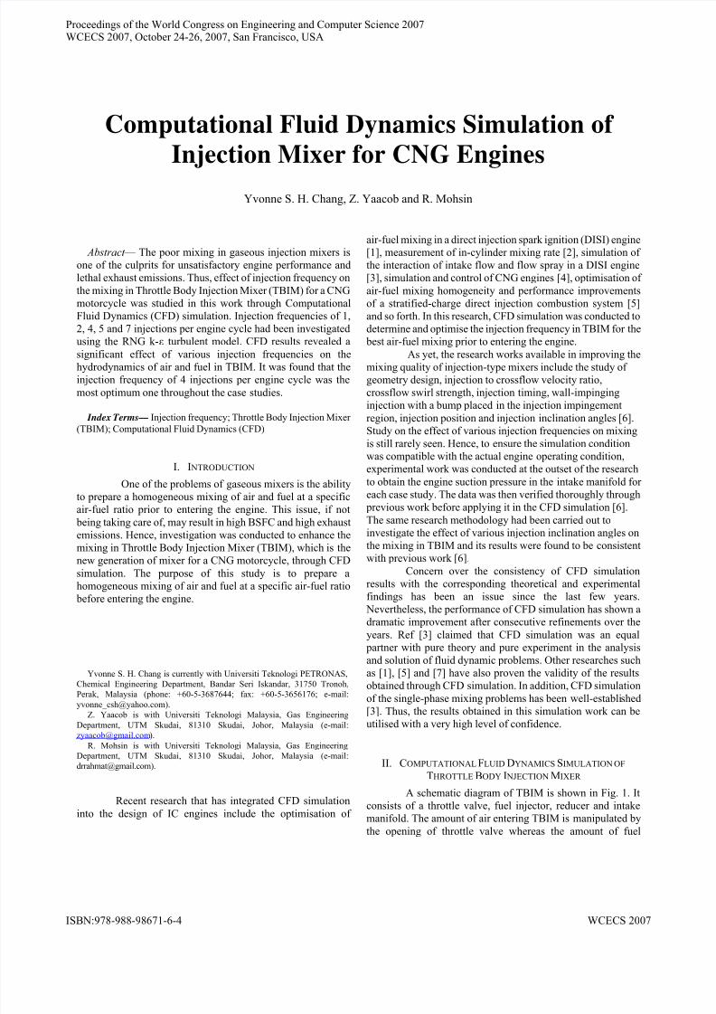
A schematic diagram of TBIM is shown in Fig. 1. It
consists of a throttle valve, fuel injector, reducer and intake
manifold. The amount of air entering TBIM is manipulated by
the opening of throttle valve whereas the amount of fuel
Computational Fluid Dynamics Simulation of
Injection Mixer for CNG Engines Yvonne S. H. Chang, Z. Yaacob and R. Mohsin
Proceedings of the World Congress on Engineering and Computer Science 2007WCECS 2007, October 24-26, 2007, San Francisco, USA
ISBN:978-988-98671-6-4 WCECS 2007
8/7/2019 simulation TBI mixer
http://slidepdf.com/reader/full/simulation-tbi-mixer 2/6
required is controlled by the fuel injector. The air and fuel are
mixed in TBIM before entering the engine. In this work, the
fuel was injected at various injection frequencies, i.e. 1, 2, 4, 5
and 7 injections per engine cycle to study its effect on the
mixing in TBIM. CFD simulation of TBIM commenced with
model meshing, followed by the optimisation of grids andselection of turbulent model before starting the computation.
Fig. 1: Outline of TBIM
II.1 Model Meshing
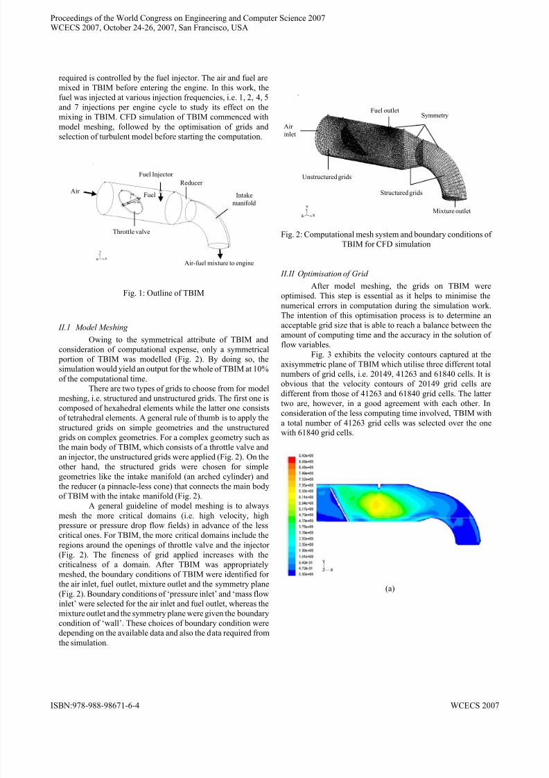
Owing to the symmetrical attribute of TBIM and
consideration of computational expense, only a symmetrical
portion of TBIM was modelled (Fig. 2). By doing so, the
simulation would yield an output for the whole of TBIM at 10%
of the computational time.There are two types of grids to choose from for model
meshing, i.e. structured and unstructured grids. The first one is
composed of hexahedral elements while the latter one consists
of tetrahedral elements. A general rule of thumb is to apply the
structured grids on simple geometries and the unstructured
grids on complex geometries. For a complex geometry such as
the main body of TBIM, which consists of a throttle valve and
an injector, the unstructured grids were applied (Fig. 2). On the
other hand, the structured grids were chosen for simple
geometries like the intake manifold (an arched cylinder) and
the reducer (a pinnacle-less cone) that connects the main body
of TBIM with the intake manifold (Fig. 2).
A general guideline of model meshing is to always
mesh the more critical domains (i.e. high velocity, high
pressure or pressure drop flow fields) in advance of the less
critical ones. For TBIM, the more critical domains include the
regions around the openings of throttle valve and the injector
(Fig. 2). The fineness of grid applied increases with the
criticalness of a domain. After TBIM was appropriately
meshed, the boundary conditions of TBIM were identified for
the air inlet, fuel outlet, mixture outlet and the symmetry plane
(Fig. 2). Boundary conditions of ‘pressure inlet’ and ‘mass flow
inlet’ were selected for the air inlet and fuel outlet, whereas the
mixture outlet and the symmetry plane were given the boundary
condition of ‘wall’. These choices of boundary condition were
depending on the available data and also the data required from
the simulation.
Fig. 2: Computational mesh system and boundary conditions of
TBIM for CFD simulation
II.II Optimisation of Grid
After model meshing, the grids on TBIM were
optimised. This step is essential as it helps to minimise the
numerical errors in computation during the simulation work.
The intention of this optimisation process is to determine an
acceptable grid size that is able to reach a balance between the
amount of computing time and the accuracy in the solution of
flow variables.
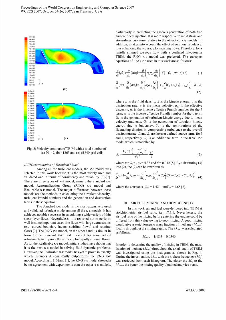
Fig. 3 exhibits the velocity contours captured at the
axisymmetric plane of TBIM which utilise three different total
numbers of grid cells, i.e. 20149, 41263 and 61840 cells. It is
obvious that the velocity contours of 20149 grid cells aredifferent from those of 41263 and 61840 grid cells. The latter
two are, however, in a good agreement with each other. In
consideration of the less computing time involved, TBIM with
a total number of 41263 grid cells was selected over the one
with 61840 grid cells.
Throttle valve
Fuel Injector
Intake
manifold
Reducer
Air Fuel
Air-fuel mixture to engine
Air inlet
Mixture outlet
Fuel outletSymmetry
Structured grids
Unstructured grids
(a)
Proceedings of the World Congress on Engineering and Computer Science 2007WCECS 2007, October 24-26, 2007, San Francisco, USA
ISBN:978-988-98671-6-4 WCECS 2007
8/7/2019 simulation TBI mixer
http://slidepdf.com/reader/full/simulation-tbi-mixer 3/6
Fig. 3: Velocity contours of TBIM with a total number of
(a) 20149, (b) 41263 and (c) 61840 grid cells
II.III Determination of Turbulent Model
Among all the turbulent models, the κ -ε model was
selected in this work because it is the most widely used and
validated one in terms of consistency and reliability [8]-[9].
There are three types of κ -ε model, namely the Standard κ -ε
model, Renormalization Group (RNG) κ -ε model and
Realizable κ -ε model. The major differences between these
models are the methods in calculating the turbulent viscosity,
turbulent Prandtl numbers and the generation and destruction
terms in the ε equation.
The Standard κ -ε model is the most extensively used
and validated turbulent model among all the κ -ε models. It hasachieved notable successes in calculating a wide variety of thin
shear layer flows. Nevertheless, it is reported not to perform
well in some important cases like flows with large extra strains
(e.g. curved boundary layers, swirling flows) and rotating
flows [9]. The RNG κ -ε model, on the other hand, is similar in
form to the Standard κ -ε model, except for some added
refinements to improve the accuracy for rapidly strained flows.
As for the Realizableκ -ε model, initial studies have shown that
it is the best κ -ε model in solving fluid dynamic problems.
However, the Realizable κ -ε model has yet to prove in exactly
which instances it consistently outperforms the RNG κ -ε
model. According to [10] and [1], the RNG k-ε model showed a
better agreement with experiments than the other κ -ε models,
particularly in predicting the gaseous penetration of both free
and confined injection. It is more responsive to rapid strain and
streamlines curvature relative to the other two κ -ε models. In
addition, it takes into account the effect of swirl on turbulence,
thus enhancing the accuracy for swirling flows. Therefore, for a
rapidly strained gaseous flow with a confined injection inTBIM, the RNG κ -ε model was preferred. The transport
equations of RNG κ -ε used in this work are as follows:
where ρ is the fluid density, k is the kinetic energy, ε is the
dissipation rate, u is the mean velocity, μeff is the effectiveviscosity, αk is the inverse effective Prandlt number for the k
term, αε is the inverse effective Prandlt number for the ε term,
Gk is the generation of turbulent kinetic energy due to mean
velocity gradients, Gb is the generation of turbulent kinetic
energy due to buoyancy, Y m is the contributions of the
fluctuating dilation in compressible turbulence to the overall
dissipation rate, S k and S ε are the user defined source terms for k
and ε, respectively. Rε is an additional term in the RNG κ -ε
model which is modelled by:
where η = S k / ε , η0 = 4.38 and β = 0.012 [8]. By substituting (3)
into (2), the (2) can be rewritten as:
where the constants C 1e = 1.42 andC 2e = 1.68 [8].
III. AIR FUEL MIXING AND HOMOGENEITY
In this work, air and fuel were delivered into TBIM atstoichiometric air-fuel ratio, i.e. 17.3:1. Nevertheless, the
air-fuel ratio of the mixing before entering the engine could be
differed from this value owing to poor mixing. A good mixing
would give a stoichiometric mass fraction of methane (M ch4.s)
locally throughout the mixing region. The M ch4.s was calculated
as follows:
M ch4.s = 1/18.3 = 0.0546
In order to determine the quality of mixing in TBIM, the mass
fraction of methane (M ch4) throughout the axial length of TBIM
was investigated using the histogram as shown in Fig. 4.
During the investigation, M ch4 with the highest frequency (M hf )
was retrieved from each histogram. The closer the M hf to the
M ch4.s, the better the mixing quality obtained and vice versa.
(c)
(b)
( ) ( ) k mbk
j
eff k
j
i
i
S Y GGx
k
xku
xk
t +−−++
⎟⎟
⎠
⎞
⎜⎜
⎝
⎛
∂
∂
∂
∂=
∂
∂+
∂
∂ρε μ α ρ ρ
( ) ( ) ( ) eebk
j
eff
j
i
i
S Rk
C GC Gk
C xx
uxt
+−−++⎟⎟
⎠
⎞
⎜⎜
⎝
⎛
∂
∂
∂
∂=
∂
∂+
∂
∂2
231
ε ρ
ε ε μ α ρε ρε ε ε ε ε
(2)
(1)
k
C
R2
3
2
0
3
1
1ε
βη
ε η
η ρη μ
ε ⋅
+
⎟⎠⎞
⎜⎝ ⎛
−
= (3)
( ) ( ) ( )k
C GC Gk
C xx
uxt
ebk e
j
e
j
i
i
2
231ε ρ
ε ε μ α ρε ρε ε ε
∗−++
⎟⎟
⎠
⎞
⎜⎜
⎝
⎛
∂
∂
∂
∂=
∂
∂+
∂
∂
(4)
Proceedings of the World Congress on Engineering and Computer Science 2007WCECS 2007, October 24-26, 2007, San Francisco, USA
ISBN:978-988-98671-6-4 WCECS 2007

8/7/2019 simulation TBI mixer
http://slidepdf.com/reader/full/simulation-tbi-mixer 4/6
Fig. 4: Histogram of M ch4 used to determine M hf
In addition, the quality of mixing was also investigated
through the mixing homogeneity (H m) in TBIM. The H m wasdefined as the ability of air and fuel to mix with a uniform M ch4
in TBIM. To justify the H m more effectively, the quality of H m
had been standardized and graded according to the number of
contours of M ch4 in the mixing region (Fig. 5). The best H m, i.e.
Grade A, was exhibited by merely one contour of M ch4.
However, if it happened to have two contours of M ch4 instead of
one, Grade B would be considered. As for Grade C, it was
signified by a total of three contours of M ch4 in the mixing
region concerned. Finally, the worst H m, which had four or
more contours of M ch4 in the mixing region concerned, was
represented by Grade D.
Fig. 5: Standardization of quality of H m with (a) Grade
A, (b) Grade B, (c) Grade C and (d) Grade D
IV. EFFECT OF INJECTION FREQUENCIES ON MHF Fig. 6 shows the effect of various injection frequencies
on M hf throughout the case studies at different engine speeds
and throttle openings. The injection frequencies studied were 1
(1if), 2 (2if) and 4 (4if) injections per engine cycle. On the
whole, the M hf at 4if showed the lowest value compared to the
other two smaller injection frequencies. The lower the M hf , the
closer it was to the M ch4.s, and thus the better the mixing quality.
Hence, injection frequency at 4if exhibited the best mixing
quality in TBIM.
Mhf
Frequency of o
ccurrence
Mch4 throu hout the axial len th of TBIM(c)
(d)
(a)
(b)
0.11
0.12
0.13
0.14
0.15
0.16
0.17
0.18
0.19
0.2
0 1 2 3 4 5
Injection Frequency
Mhf
0 deg throttle angle
5 deg throttle angle
10 deg throttle angle
15 deg throttle angle
20 deg throttle angle
25 deg throttle angle
30 deg throttle angle
(a)
Proceedings of the World Congress on Engineering and Computer Science 2007WCECS 2007, October 24-26, 2007, San Francisco, USA
ISBN:978-988-98671-6-4 WCECS 2007

8/7/2019 simulation TBI mixer
http://slidepdf.com/reader/full/simulation-tbi-mixer 5/6
Fig. 6: M hf vs injection frequency at (a) 1680 rpm, (b)
2160 rpm, (c) 4500 rpm and (d) 7200 rpm
The effect of injection frequency on the mixing in
TBIM was strongly related to the sustainability of injection
momentum and mixing energy. By applying more than one
injection per engine cycle in the TBIM, a much greater turbulent intensity could be achieved as the injection took place
intermittently [11]. Hence, the sustainability of injection
momentum and mixing energy were increased. In this way, the
mixture was able to mix thoroughly owing to the adequate
mixing energy provided periodically. As a result, the M hf
decreased with increasing injection frequencies.
V. EFEECT OF INJECTION FREQUENCIES ON HM
Unlike the M hf , the H m obtained at different injection
frequencies for all the case studies were quite compatible and
no significant enhancement on the H m could be seen. This was
shown by the number of case studies obtained for each grade of
H m in Table 1. This might due to inadequate distribution of
mixing energy which was governed by other parameters suchas the injection position, injection inclination angle [12] as well
as crossflow of air into TBIM [13]-[14].
Table 1: Number of case studies obtained for each grade of H m
VI. OPTIMISATION OF INJECTION FREQUENCY
To obtain the optimum injection frequency for the best
mixing quality, further investigation was conducted for 5if
(5-injection/engine cycle) and 7if (7-injection/engine cycle) on
selected case studies. As shown in Fig. 7, the M hf at 4if
generally showed the lowest value which was closest to M ch4.s
relative to the other injection frequencies studied. Thus, 4if
gave the best mixing at M ch4.s. For the H m, on the other hand, it
was evident that the H m obtained at 1if and 4if were
comparatively better than those obtained at 2if (Table 1). The
former ones had 9 and 8 case studies for Grade A while the
latter one had only 4 case studies, as shown in Table 1.
Determination of the best H m obtained between 1if and 4if was
rather difficult as they showed nearly the same number of case
studies for Grade A. Nonetheless, an obvious variation of the
number of case studies obtained for Grade B and Grade C could
be seen. Since 4if produced a larger number of case studies for
Grade B and a fewer for Grade C, it was claimed to be a better
injection frequency for H m than 1if. Therefore, it could be
concluded that the optimum injection frequency of TBIM for
the best H m with M ch4 closed to M ch4.s was 4if.
Fig. 7: M hf vs injection frequency at 30 degree throttle opening
for different engine speeds
Grades of Hm Injection frequency
A B C D
1if 9 12 7
2if 4 17 7
4if 8 19 1
0.05
0.07
0.09
0.11
0.13
0.15
0.17
0.19
0.21
0 1 2 3 4 5 6 7 8
Injection Frequency
Mh
f1680rpm
2160rpm
4500rpm
7200rpm
0.08
0.1
0.12
0.14
0.16
0.18
0 1 2 3 4 5
Injection Frequency
Mhf
0 deg throttle angle
5 deg throttle angle
10 deg throttle angle
15 deg throttle angle
20 deg throttle angle
25 deg throttle angle
30 deg throttle angle
0.06
0.070.08
0.09
0.1
0.11
0.12
0.13
0 1 2 3 4 5
Injection Frequency
Mhf
30 deg throttle angle
40 deg throttle angle
50 deg throttle angle
60 deg throttle angle
70 deg throttle angle
80 deg throttle angle
90 deg throttle angle
(b)
0.055
0.06
0.065
0.07
0.075
0.08
0.085
0.09
0 1 2 3 4 5
Injection Frequency
Mhf
30 deg throttle angle
40 deg throttle angle
50 deg throttle angle
60 deg throttle angle
70 deg throttle angle
80 deg throttle angle
90 deg throttle angle
(c)
(d)
Proceedings of the World Congress on Engineering and Computer Science 2007WCECS 2007, October 24-26, 2007, San Francisco, USA
ISBN:978-988-98671-6-4 WCECS 2007
8/7/2019 simulation TBI mixer
http://slidepdf.com/reader/full/simulation-tbi-mixer 6/6
VII. CONCLUSION
The effect of various injection frequencies on the
mixing quality of TBIM in terms of M hf and H m had been
studied in this research. A good mixing was that with M hf
closed to M ch4.s and the best H m at the same time, which was
shown by a single contour of M ch4 throughout the mixing regionduring CFD simulation. Although the H m was not improved
remarkably, the M hf was, however, enhanced dramatically with
a varying injection frequency. The optimum injection
frequency for both M hf and H m throughout the case studies was
found to be at 4if. Future studies on the effect of other
parameters such as injection position, injection inclination
angle as well as crossflow of air into TBIM should be
conducted to further enhance the air-fuel mixing prior to
entering the engine.
ACKNOWLEGMENT
We wish to record our sincere gratitude to UniversitiTeknologi PETRONAS (UTP) and Universiti Teknologi
Malaysia (UTM). Apart from financial support, they made
available to us research facilities and resources which were
integral to this work. In addition, unstinting technical assistance
from Mr. King Ik Piau., Mr Yeap Beng Hi, Mr. Chin Vee Dee,
En. Rosdi Baharim, En. Mohd Redhuan Ramli and En. Faizal
Ali Othman is greatly acknowledged.
REFERENCES
[1] Papageorgakis, G. and Assanis, D. N. (1998). Optimizing Gaseous Fuel-Air
Mixing in Direct Injection Engines Using an RNG Based k-ε Model. SAE
Technical Paper Series. SAE 980135.[2] Lacher, S. J., Fan, L., Backer, B., Martin, J. K., Reitz, R., Yang, J. and
Anderson, R. (1999). In-Cylinder Mixing Rate Measurements and CFD
Analyses. SAE Technical Paper Series. SAE 1999-01-1110.
[3] Anderson, R., Yi, J., Han, Z., Yang, J., Trigui, N., and Boussarsar, R.
(2000). Modeling of the Interaction of Intake Flow and Fuel Spray in DISI
Engines. SAE Technical Paper Series. SAE 2000-01-0656.
[4] Dyntar, D., Onder, C. and Guzzella, L. (2002). Modeling and Control of
CNG Engines. SAE Technical Paper Series. SAE 2002-01-1295.
[5] Yi, J., Han, Z. and Trigui, N. (2002) Fuel-Air Mixing Homogeneity and
Performance Improvements of a Stratified-Charge DISI Combustion
System. SAE Technical Paper Series. SAE 2002-01-2656.
[6] Chang, S. H. Effect of Injection Characteristics on Throttle Body Injection
Mixer for Compressed Natural Gas Motorcycle. Universiti Teknologi
Malaysia. Malaysia: M. Eng. Thesis.
[7] Yi, J., Han, Z., Yang, J., Anderson, R., Trigui, N. and Boussarsar, R. (2000).
Modeling of the Interaction of Intake Flow and Fuel Spray in DISI Engines.SAE Technical Paper Series. SAE 2000-01-0656.
[8] Fluent Inc. (2001). Fluent 6 User’s Guide. India: Fluent Documentation
Software.
[9] Versteeg, H. K. and Malalasekera, W. 1999. An Introduction to
Computational Fluid Dynamics – The Finite Volume Method . England:
Longman Group Ltd.
[10] Han, Z. and Reitz, R. D. (1995). Turbulence Modeling of Internal
Combustion Engines Using RNG k-e Models. Comb. Sci. & Tech. Vol
(106): 267-295.
[11] Christian, F. 1996. Experimental Study of Mixing Performances Using
Steady and Unsteady Jets. In: Cheremisinoff, N. P. ed. Mixed-Flow
Hydrodynamics – Advances in Engineering Fluid Mechanics Series .
Texas: Gulf Publishing Company. 359-381.
[12] Tatterson, G. B. 1994. Scaleup and Design of Industrial Mixing Process.
United States of America: McGraw-Hill.
[13] Busnaina, A. A. 1985. Transient Predictions of Lateral Jet Injection intoTypical Isothermal Combustor Flowfields. AIAA 23rd Aerospace Sciences
Meeting . January 14-17. Nevada: American Institute of Aeronautics and
Astronautics, 1-9.
[14] Ferrell, G. B., Aoki, K. and Lilley, D. G. 1985. Flow Visualization of
Lateral Jet Injection into Swirling Crossflow. AIAA 23rd Aerospace
Sciences Meeting . January 14-17. Nevada: American Institute of
Aeronautics and Astronautics, 1-10.
Proceedings of the World Congress on Engineering and Computer Science 2007WCECS 2007, October 24-26, 2007, San Francisco, USA
ISBN:978-988-98671-6-4 WCECS 2007


![[Files.indowebster.com] TBI](https://static.fdocuments.in/doc/165x107/577cd9c51a28ab9e78a423d2/filesindowebstercom-tbi.jpg)