SIMULATION STUDY OF 1DOF HYBRID ADAPTIVE CONTROL APPLIED ON ISOTHERMAL CONTINUOUS STIRRED-TANK REACTOR

Jiri Vojtesek, Lubos Spacek and Petr Dostal

Faculty of Applied Informatics Tomas Bata University in Zlin

Nam. TGM 5555, 760 01 Zlin, Czech Republic E-mail: {vojtesek,lspacek}@fai.utb.cz

KEYWORDS Simulation, Mathematical Model, Adaptive Control, Continuous Stirred-Tank Reactor, 1DOF, Polynomial Approach. ABSTRACT

A Continuous Stirred-Tank Reactor is typical system with nonlinear behavior and lumped parameters. The mathematical model of this type of reactor is described by the set of nonlinear ordinary differential equations that are easily solvable with the use of numerical methods. The big advantage of the computer simulation is that once we have reliable mathematical model of the system we can do thousands of simulation experiments that are quicker, cheaper and safer then examination on the real system. The control approach used in this work is a hybrid adaptive control where an adaptation process is satisfied by the on-line recursive identification of the External Linear Model as a linear representation of the originally nonlinear system. The polynomial approach together with the Pole-placement method and spectral factorization satisfies basic control requirements such as a stability, a reference signal tracking and a disturbance attenuation. Moreover, these methods produce also relations for computing of controller’s parameters. As a bonus, the controlled output could be affected by the choice of the root position in the Pole-placement method. The goal of this contribution is to show that proposed controller could be used for various outputs as this system provides five possible options.

INTRODUCTION

The mathematical modelling and the computer simulation is a great tool for control engineering that helps with the understanding of the system’s behavior without exanimation on a real equipment or a real model of the system (Honc et al. 2014), (Ingham et al. 2000). The benefits of the computer simulation are clear – it is quick, safe and of course much cheaper method than real experiments which, especially in chemical industry, could consume a lot of chemicals without a clear result. Even more, a lot of chemical experiments produce an exothermic reaction and wrong settings of the controller could end with the dangerous explosion. This paper presents the simulation study from the initial steady-state and dynamic analyses to the hybrid

adaptive control of the system. The steady-state and dynamic analyses observes the nonlinear behavior of the system and help us with the choice of the optimal control strategy. The system under the consideration is an isothermal Continuous Stirred-Tank Reactor (CSTR) the mathematical model of which is described by the set of five nonlinear ordinary differential equations (ODE) as there are five state variables – concentrations (Russell and Denn 1972). There were used Simple iteration method for the solving of the steady-state of this system which is, in fact, the numerical solution of the set of nonlinear algebraic equations that are transformed from the set of ODE with the condition that the derivative with respect to the time are equal to the zero in the steady-state. The dynamic analysis then employs the Standard Runge-Kutta’s method for numerical solution of the set of ODE. Both methods are simple but accurate enough. Moreover, they are easily programmable and Runge-Kutta’s methods are even build-in functions in the mathematical software Matlab (Vojtesek 2014) which was used as a simulation program in this work. The control method here is based on the idea of the adaptive control (Åström and Wittenmark, 1989) where parameters of the controller are restored during the control according to the actual needs and state of the controlled system. The core function of this adaptive approach is the recursive identification of the External Linear Model (ELM) as a linear representation of the nonlinear system (Bobal et al., 2005). Parameters of the controller than depends on the identified ELM and they are computed with the use the Polynomial method, the Pole-placement method and the Spectral factorization. As a result, this approach produces not only the controller that satisfies basic control requirements but also easily programmable relations for computing of controller’s parameters which helps with the implementation inside the industrial controllers. We call this approach the “hybrid” adaptive control because the polynomial approach used here is defined in the continuous-time which is more accurate but problematic for the on-line identification. Because of this, the special type of the discrete-time identification was used. This method is called the Delta-models (Middleton and Goodwin 2004) that belongs to the class of discrete-time models but its parameters approaches to the continuous-time ones for sufficiently small sampling

Proceedings 31st European Conference on Modelling and Simulation ©ECMS Zita Zoltay Paprika, Péter Horák, Kata Váradi, Péter Tamás Zwierczyk, Ágnes Vidovics-Dancs, János Péter Rádics (Editors) ISBN: 978-0-9932440-4-9/ ISBN: 978-0-9932440-5-6 (CD)

period (Stericker and Sinha 1993) as there are both input and output variables related to the sampling period. The control strategy was applied on the control of two different outputs which shows that it could be also successfully applicable to similar types of processes.

ADAPTIVE CONTROL

The control approach used in this work is an adaptive control. The philosophy of this control method comes from the nature, where plants, animals and even human beings “adopt” their behavior to the actual conditions and an environment. This could be done, from the control point of the view, for example by the change of the controller’s parameters, structure etc. (Bobal et al., 2005).

External Linear Model

The approach used here starts with the dynamic analysis of the system that help us with the understanding of the system’s behavior. Resulted step responses are then used for the choice of the External Linear Model (ELM) as a linear representation of usually nonlinear system. This ELM could be in the form of the polynomial transfer function and the adaptivity is then satisfied by on-line recursive identification that estimates parameters of the ELM in every moment. This procedure guarantees that this ELM describes the system accurately to the relative state of the system. The general form of the ELM’s transfer function is

( )( )

( )b s

G sa s

= (1)

where parameters of polynomials a(s) and b(s) are computed from the recursive identification and both polynomials holds the feasibility condition for

( ) ( )deg dega s b s≥ .

Design of Controller

Now we know, that the controlled nonlinear system is described by the polynomial transfer function (1) and we can describe the controller also by the transfer function

( ) ( )( )

q sQ s

p s= (2)

where q(s) and p(s) are again commensurable polynomials with the properness condition ( ) ( )deg degp s q s≥ .

Figure 1: 1DOF control scheme

If we put this controller’s transfer function in the feedback part of the closed-loop scheme displayed in Figure 1, the Laplace transform of the transfer function G(s) in (1) is then

( ) ( )( ) ( ) ( ) ( )

Y sG s Y s G s U s

U s= ⇒ = ⋅ (3)

where Laplace transform of the input signal u is from Figure 1

( ) ( ) ( ) ( ) ( ) ( ) ( ) ( )U s Q s E s V s Q s W s Y s V s= ⋅ + = ⋅ − +⎡ ⎤⎣ ⎦ (4)

Then, if we put polynomials a(s), b(s), p(s) and q(s) from (1) and (2), the equation (3) has form

( ) ( ) ( )( ) ( ) ( ) ( ) ( )

( ) ( )( ) ( ) ( ) ( ) ( )

b s q sY s W s

a s p s b s q s

a s p sV s

a s p s b s q s

= ⋅ ++

+ ⋅+

…

… (5)

The denominator here is a characteristic polynomial of the closed loop system we can write it generally

( ) ( ) ( ) ( ) ( )a s p s b s q s d s⋅ + ⋅ = (6)

where d(s) is a stable optional polynomial. The position of roots of this polynomial affects control results and the whole equation (6) is called Diophantine equation (Kucera 1993). Every control system must fulfill basic control requirements such as a stability, an asymptotic tracking of the reference signal and the disturbance attenuation. The closed loop system is stable, if the polynomial d(s) on the left side of (6) is also stable. Asymptotic tracking of the reference signal and disturbance attenuation is gained if the polynomial p(s) includes the least common divisor f(s) of denominators of transfer functions of the reference signal w and disturbance signal v:

( ) ( ) ( )p s f s p s= ⋅ (7)

As both of these signals are expected as a step function, the least common divisor is f(s) = s. The transfer function of the feedback controller is then

( ) ( )( )

q sQ s

s p s=

⋅(8)

and we can rewrite the Diophantine equation (6) to

( ) ( ) ( ) ( ) ( )a s s p s b s q s d s⋅ ⋅ + ⋅ = (9)

Polynomials a(s) and b(s) are known from the recursive identification and polynomials ( )p s and q(s) are unknown parameters that are needed to be computed. The method used here for computation of those polynomials is the Method of uncertain coefficients. The polynomial d(s) on the right side of the equation (9) is the stable optional polynomial. The simple method

used for the choice of the polynomial d(s) is the Pole-placement method which divides this polynomial into one or more parts with double, triple, etc. roots, e.g.

( ) ( ) ( ) ( ) ( )/2 / 21 2; ,m m md s s d s s sα α α= + = + ⋅ + … (10)

where α > 0. The disadvantage of this method can be found in the uncertainty. There is no general rule which can help us with the choice of roots which are, of course, different for different controlled processes. One way how we can overcome this unpleasant feature is to use spectral factorization. Big advantage of this method is that it can make stable roots from every polynomial, even if it is unstable. The polynomial d(s) is in this case

( ) ( ) ( ) ( ) ( )deg degd s n sd s n s s α −= ⋅ + (11)

where parameters of the polynomial n(s) are computed from the spectral factorization of the polynomial a(s) in the denominator of (1), i.e.

( ) ( ) ( ) ( )* *n s n s a s a s⋅ = ⋅ (12)

The use of the spectral factorization satisfies that the polynomial n(s) is stable even if the identified polynomial a(s) is unstable. This situation could occur in the adaptation part at the beginning of the control, where the estimator does not have enough information about the system. The second part is then regular Pole-placement method, but the number of unknown roots is reduced by the choice of the polynomial n(s). It is good to have some parameter that could affect the control results. This parameter is in this case the position of the root α in the Pole-placement method. The only condition which comes from the stability is that this root must be α > 0. Degrees of unknown polynomials ( )p s , q(s) and d(s) are for the fulfilled properness condition generally:

( ) ( )( ) ( )( ) ( ) ( )( ) ( )

deg deg 1

deg deg

deg deg deg 1

deg deg

p s a s

q s a s

d s a s p s

n s a s

≥ −

=

= + +

=

(13)

Recursive Identification

The computation of the controller’s parameters by the Method of uncertain coefficients needs parameters of the system, i.e. coefficients of polynomials a(s) and b(s) from the transfer function G(s) in (1). It was mentioned before, that these coefficients are estimated recursively during the control. The Recursive Least-Squares (RLS) method (Rao and Unbehauen 2005) is ideal method for this task – it is easily programmable and together with forgetting factors accurate enough. The RLS method uses two vectors: the first is data vector that comes from the measured input and output variables, generally in the discrete form

[

]( 1) ( 1), ( 2), , ( )

( 1), ( 2), , ( ) T

k y k y k y k n

u k u k u k m

− = − − − − − −

− − −

…

…

ϕ (14)

The second, unknown, vector is the vector of parameters

( ) [ ]1 0 1 0, , , , , , , Tn mk a a a b b b= … …θ (15)

and this vector is in RLS computed from the set of equations:

( ) ( ) ( ) ( )

( ) ( ) ( ) ( )( ) ( ) ( ) ( )

( ) ( ) ( ) ( ) ( ) ( ) ( )( )( ) ( ) ( ) ( )

( ) ( ) ( ) ( )

1

11

2

ˆ 1

1 1

1

1 11 111

11

ˆ ˆ 1

T

T

T

T

k y k k k

k k k k

k k k k

k k k kk k

kkk k k

k

k k k k

ε

γ

γ

λλλ

ε

−

= − ⋅ −

⎡ ⎤= + ⋅ − ⋅⎣ ⎦= ⋅ − ⋅

⎡ ⎤⎢ ⎥− ⋅ ⋅ ⋅ −⎢ ⎥= − −⎢ ⎥−−

+ ⋅ − ⋅⎢ ⎥−⎢ ⎥⎣ ⎦

= − +

P

P

P PP P

P

L

L

ϕ θ

ϕ ϕ

ϕ

ϕ ϕ

ϕ ϕ

θ θ

(16)

where ϕ is regression vector, ε denotes a prediction error, P is a covariance matrix and λ1 and λ2 are forgetting factors. There were defined different methods in (Fikar and Mikles 1999), for example constant exponential forgetting where λ2 = 1 and λ1 is computed from

( ) ( ) ( )21 1k K k kλ γ ε= − ⋅ ⋅ (17)

where K is a very small value (e.g. K = 0.001). SIMULATION MODEL

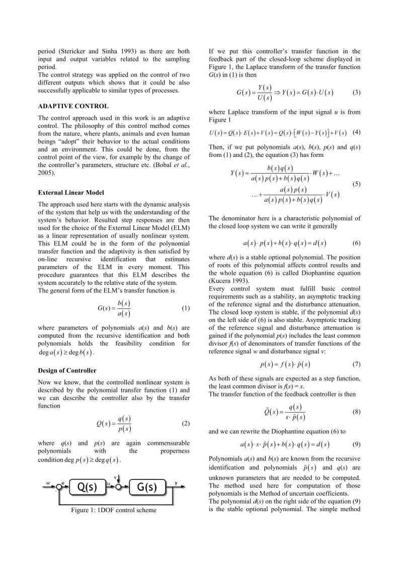
The proposed adaptive control was tested by the simulation on the mathematical model of the isothermal chemical reactor (Russell and Denn 1972), schematic representation of which is shown in Figure 2.

Figure 2: Isothermal Continuous Stirred-Tank Reactor Reactions inside the reactor are

31 2; ; kk kA B X A X Y A Y Z+ ⎯⎯→ + ⎯⎯→ + ⎯⎯→ (18)

The mathematical model is constructed with the use of material balances, that are in the general word form

Mass flow of the Mass flow of the Rate ofcomponent into component out of accumulation of

the system the system mass in the system

⎧ ⎫ ⎧ ⎫ ⎧ ⎫⎪ ⎪ ⎪ ⎪ ⎪ ⎪= +⎨ ⎬ ⎨ ⎬ ⎨ ⎬⎪ ⎪ ⎪ ⎪ ⎪ ⎪⎩ ⎭ ⎩ ⎭ ⎩ ⎭and as we have five state variables – concentrations cA, cB, cX, cY and cZ, the resulting mathematical model is described by five ordinary differential equations (Russell and Denn 1972)

( )

( )

( )

( )

( )

0 1

0 1

2 3

0 1 2

0 2 3

0 3

AA A A B

BB B A B

B X B Y

XX X A B B X

YY Y B X B Y

ZZ Z B Y

dc q c c k c cdt V

dc q c c k c cdt V

k c c k c cdc q c c k c c k c cdt V

dc q c c k c c k c cdt V

dc q c c k c cdt V

= − − ⋅ ⋅

= − − ⋅ ⋅ −

− ⋅ ⋅ − ⋅ ⋅

= − + ⋅ ⋅ − ⋅ ⋅

= − + ⋅ ⋅ − ⋅ ⋅

= − + ⋅ ⋅

(19)

The mathematical model (19) includes besides state variables cA, cB, cX, cY and cZ also their initial values (with index c·0), volumetric flow rate q, volume of the reactor V and rate constants of the reactions k1 – k3. Rate constants, the volume of the reactant and input concentrations are fixed parameters that are shown in Table 1(Russell and Denn 1972):

Table 1: Fixed parameters of the CSTR k1 = 5×10-4 m3.kmol-1.s-1 k2 = 5×10-2 m3.kmol-1.s-1 k3 = 2×10-2 m3.kmol-1.s-1 V = 1 m3

cA0 = 0.4 kmol.m-3 cB0 = 0.6 kmol.m-3 cX0 = cY0 = cZ0 = 0 kmol.m-3

The only quantity which could be used as an adjustable parameter is the volumetric flow rate of the reactant q which was later used as an action value for control. The Steady-state and Dynamic Analyses

The goals of the steady-state and dynamic analyses are usually to observe the behavior of the system and its physical boundaries. The steady-state analysis tries to find values of the state variables in the steady-state, i.e. for the time t ∞. It means that the set of nonlinear ordinary differential equations (ODE) (19) is transformed into the set of nonlinear algebraic equations that can be solved for example with the Simple iteration method. We have done various computations for different input volumetric flow rates q and the results are shown for example in (Zelinka et al. 2006). Our experiments have shown nonlinear behavior and the optimal working point is qs = 1×10-4 m3.s-1. Steady-state values of the state variables for this working point are:

3 3

3 3

3

0.2407 . 0.1324 .

0.0024 . 0.0057 .

0.1513 .

s sA Bs sX Y

sZ

c kmol m c kmol m

c kmol m c kmol m

c kmol m

− −

− −

−

= =

= =

=

(20)

It was already mentioned, that there are five theoretical state variables but we have chosen only two of them to be controlled – concentrations cB

s(t) and cZs(t).

As the steady-state values of quantities are also initial values for the dynamic analysis that examine the behavior after the step change of the input variable, the output variable then starts on its steady-state value. In this work, the initial value of the output variable is subtracted from the actual value which results in step responses that starts from zero. The both outputs in this work are then

( ) ( ) ( ) ( ) 31 2; .s s

B B Z Zy t c t c y t c t c kmol m−⎡ ⎤= − = − ⎣ ⎦ (21)

where cBs and cZ

s are those values in (20). There were done eight step changes of the input variable

( ) ( ) [ ]100 %s

s

q t qu t

q−

= ⋅ (22)

and results are shown in Figure 3 and Figure 4.

0 5000 10000 15000 20000-0.16

-0.12

-0.08

-0.04

0.00

0.04

0.08100 %75 %50 %25 %

-25 %

-50 %

-75 %

y 1(t) [k

mol

.m-3]

t [s]

-100 %

Figure 3: The course of the output variable y1(t) after step changes of the input variable u(t)

0 5000 10000 15000 20000

-0.02

0.00

0.02

0.04

y 2(t) [k

mol

.m-3]

t [s]

-100 %

-75 %

-50 %

-25 %

25 %50 %75 %

-100 %

Figure 4: The course of the output variable y2(t) after step changes of the input variable u(t) Step responses in Figure 3 and Figure 4 have shown nonlinear behavior of the system and also limitations of output variables. The first output differs in the boundaries from -0.1322 (-100 %) to 0.0725 (+100 %) kmol.m-3. The second output y2(t) has boundaries from -0.0245 (+100 %) to 0.0446 (-100 %).

Results of the dynamic analysis can help us with the choice of the ELM’s transfer function (1). According to courses of the output the transfer function has a form:

( )( )

( )( )

1 02

1 0

( )Y s b s b s b

G sU s a s s a s a

+= = =

+ + (23)

SIMULATION OF ADAPTIVE CONTROL

The ELM (23) is in the continuous-time s-plain and on-line identification of those models is more accurate but also problematic that those in discrete-time, where we can read input and output variables are read only in the defined time intervals and the time before this interval can be used for the recomputation of the systems or controller parameters. One compromise could be use of the so called δ-models which are special types of discrete-time identification models, where input and output variables are related to the sampling period Tv. A new complex variable γ is computed from (Mukhopadhyay et al. 1992)

( )11v v

zT z T

γα α

−=

⋅ ⋅ + − ⋅ (24)

where z is complex variable, Tv denotes a sampling period and α is an optional parameter. It is clear, that we can obtain infinitely many models for optional parameter α from the interval 0 ≤ α ≤ 1 and a sampling period Tv, however a forward δ-model was used in this work which has γ operator computed via

10v

zT

α γ −= ⇒ = (25)

The general form of the ELM (23) is then rewritten to the general differential equation

( ) ( ) ( ) ( )a y t b u tδ δ′ ′ ′ ′= (26)

where t’ denotes discrete time and δ is the operator defined according to (25). Some previous experiments (Stericker and Sinha 1993) have shown, that parameters of polynomials a’(δ) and b’(δ) approach the parameters of the continuous-time model with decreasing value of the sampling period Tv. The relation for the actual output is derived from the (26) as

( ) ( ) ( )

( ) ( )1 0

1 0

1 2

1 2

y k a y k a y k

b u k b u kδ δ δ

δ δ

= − − − − +

+ − + − (27)

where yδ is the recomputed output to the δ-model:

2

( ) 2 ( 1) ( 2)( )

( 1) ( 2)( 1) ; ( 2) ( 2)

( 1) ( 2)( 1) ; ( 2) ( 2)

v

v

v

y k y k y ky kT

y k y ky k y k y kT

u k u ku k u k u kT

δ

δ δ

δ δ

− − + −=

− − −− = − = −

− − −− = − = −

(28)

and the data vector is then

( ) ( ) ( )

( ) ( )

1 1 , 2 ,

, 1 , 2T

k y k y k

u k u k

δ δ

δ δ

− = − − − −⎡⎣

− − ⎤⎦

…

…

φ (29)

and the vector of estimated parameters

( ) 1 0 1 0ˆ , , ,

Tk a a b bδ δ δ δ⎡ ⎤= ⎣ ⎦θ (30)

can be computed from the ARX (Auto-Regressive eXtrogenous) model

( ) ( ) ( )1Ty k k kδ δ δ= ⋅ −θ ϕ (31)

by the recursive least squares methods described in the theoretical part. As the ELM in Equation (23) is of the second order with relative order one, degrees of polynomials ( )p s , q(s) and d(s) in (13) are

( ) ( )( ) ( )( ) ( ) ( )( ) ( )

deg deg 1 2 1 1

deg deg 2

deg deg deg 1 2 1 1 4

deg deg 2

p s a s

q s a s

d s a s p s

n s a s

≥ − = − =

= =

= + + = + + =

= =

(32)

and the transfer function of the controller (8) is

( ) ( )( ) ( )

22 1 0

1 0

q s q s q s qQ s

s p s s p s p+ +

= =⋅ ⋅ +

(33)

The stable polynomial d(s) on the right side of the Diophantine equation (9) is

( ) ( ) ( ) ( ) ( )2 221 0d s n s s s n s n sα α= ⋅ + = + + ⋅ + (34)

where parameters of the polynomial n(s) are computed from the spectral factorization (12) as

2 20 0 1 1 0 0, 2 2n a n a n a= = + − (35)

and we have one tuning parameter – the position of the double root α and parameters of polynomials ( )p s , q(s) in the transfer function of the controller (33) are computed from the Diophantine equation (9) by the Method of uncertain coefficients. Simulation Results

There were done different simulation experiments for u(t) as a change of the volumetric flow rate q (22) and changes of the output concentrations cB and cZ respectively – see (21). The simulation time was 30 000 s and five step changes of the reference signal were done during this time. The sampling period was Tv = 10 s, the initial covariance matrix P(0) has on the diagonal 1·106 and starting vectors of parameters for the identification was chosen according to some previous measurements.

It is good to qualify the control results also by some quantitative criterion. In this case, we used control quality criteria Su and Sy that reflects the changes of the input variable u and the control error e = w – y. These criteria are then computed in the whole control from

( ) ( )( )

( ) ( )( )

2

2

2

1

1N

ui

N

yi

S u i u i

S w i y i

=

=

= − −

= −

∑

∑, for f

v

TN

T= (36)

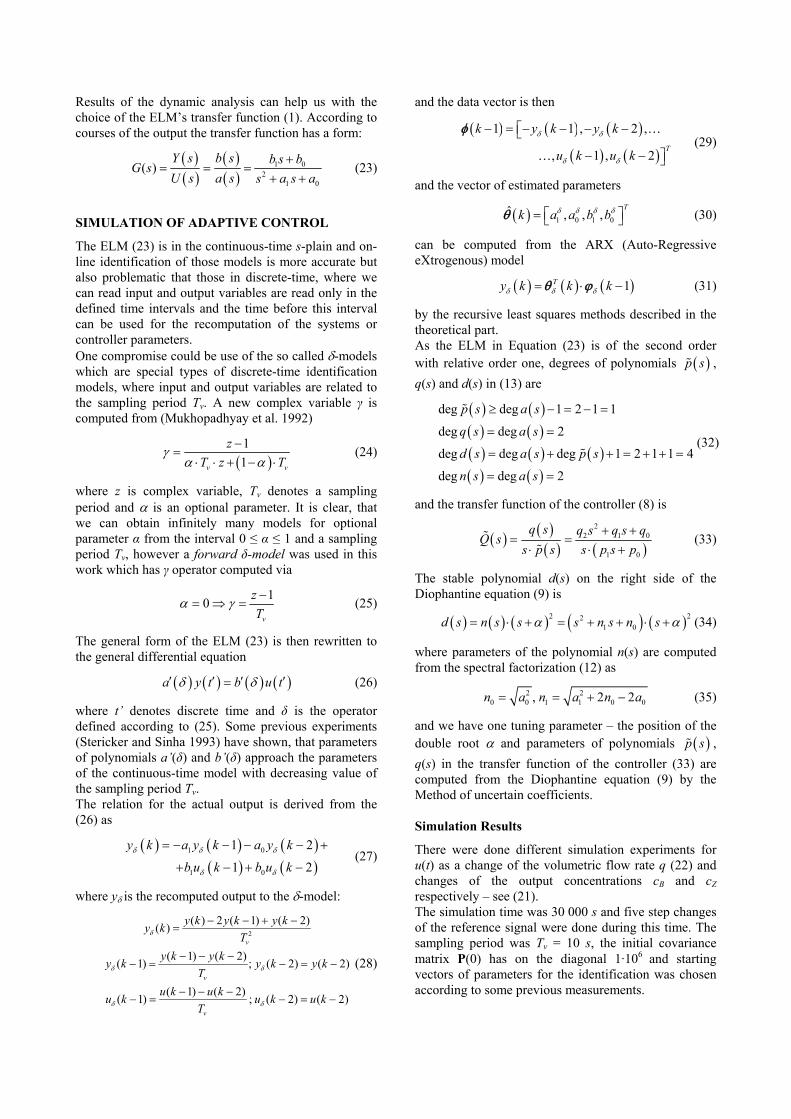
where Tf is the final time – in this case Tf = 30 000 s. The first simulation analysis observes the effect of the tuning parameter α = 0.002, 0.004 and 0.2 on the control response of the output y1(t).

0 5000 10000 15000 20000 25000 30000-0.04

-0.03

-0.02

-0.01

0.00

0.01

0.02

0.03

w(t)

, y1(

t) [k

mol

.m-3]

t [s]

w, y1 - α = 0.002, y1 - α = 0.004, y1 - α = 0.02

Figure 5: The course of the output variable y1(t) and the reference signal w(t) for various α

0 5000 10000 15000 20000 25000 30000-100

-75-50-25

0255075

100

u(t)[

%]

t [s]

u - α = 0.002 u - α = 0.004 u - α = 0.02

Figure 6: The course of the input variable u(t) in the control of the output y1(t) for various α Control results of the first simulation are shown in Figure 5 and Figure 6. It can be seen, that the proposed 1DOF hybrid adaptive controller does not have problem with the control of this output concentration cB(t). The course of the controlled output can be affected by the choice of the parameter α as a position of the root and it is clear, that bigger value of this parameter results in quicker output response but overshoot of the output variable. The question is if we want to have quicker response or overshoots are unwanted feature of the control system? The choice of the parameter α then depends on the answer for the previous question. Values of criteria Su and Sy for the first control simulation study are shown in Table 2. Lower value of α results in smoother course of the input variable which could be also important feature of the controller – quicker changes of u(t) could affect the cost of the control and moreover it could harm the hardware of the

controller that is also important. This smoother course reflects in the value of Su which is minimal for the lowest value of α – see Table 2. Table 2: Control quality criteria for the first simulation

study – control of the output y1 Su [-] Sy [kmol2.m-6]

α = 0.002 11 340 0.1554 α = 0.004 68 736 0.0777 α = 0.02 86 403 0.0636

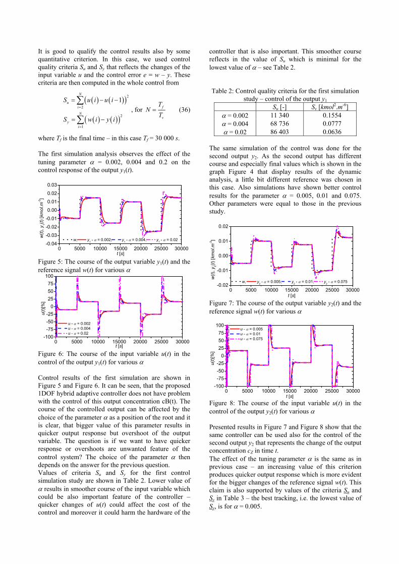
The same simulation of the control was done for the second output y2. As the second output has different course and especially final values which is shown in the graph Figure 4 that display results of the dynamic analysis, a little bit different reference was chosen in this case. Also simulations have shown better control results for the parameter α = 0.005, 0.01 and 0.075. Other parameters were equal to those in the previous study.

0 5000 10000 15000 20000 25000 30000-0.02

-0.01

0.00

0.01

0.02

w(t)

, y2(

t) [k

mol

.m-3]

t [s]

w, y2 - α = 0.005, y2 - α = 0.01, y2 - α = 0.075

Figure 7: The course of the output variable y2(t) and the reference signal w(t) for various α

0 5000 10000 15000 20000 25000 30000-100

-75-50-25

0255075

100

u(t)[

%]

t [s]

u - α = 0.005 u - α = 0.01 u - α = 0.075

Figure 8: The course of the input variable u(t) in the control of the output y2(t) for various α Presented results in Figure 7 and Figure 8 show that the same controller can be used also for the control of the second output y2 that represents the change of the output concentration cZ in time t. The effect of the tuning parameter α is the same as in previous case – an increasing value of this criterion produces quicker output response which is more evident for the bigger changes of the reference signal w(t). This claim is also supported by values of the criteria Su and Sy in Table 3 – the best tracking, i.e. the lowest value of Sy, is for α = 0.005.

Table 3: Control quality criteria for the second

simulation study – control of the output y2 Su [-] Sy [kmol2.m-6]

α = 0.005 255 704 0.0306 α = 0.01 370 423 0.0328

α = 0.075 193 016 0.0386 CONCLUSIONS

The paper shows the main benefits of the computer simulation – once we have a reliable mathematical model of the controlled system, we can do various simulations which can help us with the understanding of the behavior of the system (the steady-state and dynamic analyses) or with the choice and setting of the possible controller. The controller in this work was chosen as a hybrid adaptive controller where is the adaptivity satisfied by the recursive identification of the External Linear Model (ELM) as a linear representation of originally nonlinear system. This simplification is being supported by the on-line estimation of the ELM’s parameters. Moreover, the controller could be tuned by the choice of the parameter α and it was proofed that increasing value of parameter results in quicker output response but bigger overshoots that are usually inappropriate. Proposed results of simulations have shown that this controller can be used for this type of systems and does not matter which output you control – both controlled outputs representing changes of output concentrations of compounds B and Z indicates good control results. The only thing that differs is the choice of the reference signal which depends of the physical properties of the controlled output and the different value of α. We are then back in the main advantage of the computer simulation – while we have mathematical model and the relations that computes the parameters of the controller both in the form of simulation programs, we can do thousands of simulations that can help us with the choice of the optimal setting. REFERENCES

Åström, K.J.; Wittenmark, B. 1989. Adaptive Control. Addison Wesley. Reading. MA, 1989, ISBN 0-201-09720-6.

Bobal, V.; Böhm, J.; Fessl, J.; Machacek, J. 2005 Digital Self-tuning Controllers: Algorithms. Implementation and Applications. Advanced Textbooks in Control and Signal Processing. Springer-Verlag London Limited. 2005, ISBN 1-85233-980-2.

Fikar, M.; J. Mikles 1999. System Identification. STU Bratislava

Honc, D.; Dusek, F.; Sharma, R. 2014 “GUNT RT 010 Experimental Unit Modelling and Predictive Control Application”. In Nostradamus 2014: Prediction, Modeling and Analysis of Complex Systems. New York : Springer, 2014, s. 175-184. ISBN 978-3-319-07400-9.

Ingham, J.; Dunn, I. J.; Heinzle, E.; Prenosil, J. E. 2000 Chemical Engineering Dynamics. An Introduction to Modeling and Computer Simulation. Second. Completely

Revised Edition. VCH Verlagsgesellshaft. Weinheim, 2000. ISBN 3-527-29776-6

Kucera, V. 1993. “Diophantine equations in control – A survey”. Automatica. 29, 1993, p. 1361-1375.

Middleton, H.; Goodwin, G. C. 2004. Digital Control and Estimation - A Unified Approach. Prentice Hall. Englewood Cliffs, 2004, ISBN 0-13-211798-3

Mukhopadhyay, S.; Patra, A. G.; Rao, G. P. 1992 “New class of discrete-time models for continuos-time systems”. International Journal of Control, vol.55, 1992, 1161-1187

Rao, G. P.; Unbehauen, H. 2005 “Identification of continuous-time systems”. IEEE Process-Control Theory Application, 152, 2005, p.185-220.

Russell, T.; Denn, M. M. 1972 “Introduction to chemical engineering analysis”. New York: Wiley, 1972, xviii, 502 p. ISBN 04-717-4545-6.

Stericker, D. L.; Sinha, N. K. 1993 “Identification of continuous-time systems from samples of input-output data using the δ-operator”. Control-Theory and Advanced Technology. vol. 9, 1993, 113-125.

Vojtesek, J. 2014 “Numerical Solution of Ordinary Differential Equations Using Mathematical Software”. In Advances in Intelligent Systems and Computing. Heidelberg: Springer-Verlag Berlin, p. 213-226. ISSN 2194-5357. ISBN 978-3-319-06739-1.

Zelinka, I.; Vojtesek, J.; Oplatkova, Z. 2006. “Simulation Study of the CSTR Reactor for Control Purposes”. In: Proc. of 20th European Conference on Modelling and Simulation ESCM 2006. Bonn, Germany, p. 479-482

AUTHOR BIOGRAPHIES

JIRI VOJTESEK was born in Zlin, Czech. He studied at Tomas Bata University in Zlin, Czech Republic, where he received his M.Sc. degree in Automation and control in 2002. In 2007 he obtained Ph.D. degree in Technical

cybernetics at Tomas Bata University in Zlin. In the year 2015 he became associate professor. His research interests are modeling and simulation of continuous-time chemical processes, polynomial methods, optimal, adaptive and nonlinear control. You can contact him on e-mail address vojtesek@fai.utb.cz.

LUBOS SPACEK studied at the Tomas Bata University in Zlín, Czech Republic, where he obtained his master’s degree in Automatic Control and Informatics in 2016. He currently attends PhD study at the Department of Process Control. His e-

mail address is lspacek@fai.utb.cz.

PETR DOSTAL studied at the Technical University of Pardubice. He obtained his PhD. degree in Technical Cybernetics in 1979 and he became professor in Process Control in 2000. His research interest are

modelling and simulation of continuous-time chemical processes. polynomial methods. optimal. adaptive and robust control. Unfortunatelly, prof. Dostal has died in January 2017.