Louisiana State UniversityLSU Digital Commons

LSU Master's Theses Graduate School

2001

Simulation study and instability of adaptive controlZhongshan WuLouisiana State University and Agricultural and Mechanical College, zwu@ece.lsu.edu

Follow this and additional works at: https://digitalcommons.lsu.edu/gradschool_theses

Part of the Electrical and Computer Engineering Commons

This Thesis is brought to you for free and open access by the Graduate School at LSU Digital Commons. It has been accepted for inclusion in LSUMaster's Theses by an authorized graduate school editor of LSU Digital Commons. For more information, please contact gradetd@lsu.edu.

Recommended CitationWu, Zhongshan, "Simulation study and instability of adaptive control" (2001). LSU Master's Theses. 3603.https://digitalcommons.lsu.edu/gradschool_theses/3603

SIMULATION STUDY AND INSTABILITY OF ADAPTIVE CONTROL

A Thesis

Submitted to the Graduate Faculty of the Louisiana State University and

Agricultural and Mechanical College in partial fulfillment of the

requirements for the degree of Master of Science in Electrical Engineering

in

The Department of Electrical and Computer Engineering

by Zhongshan Wu

B.S.E.E., Northeastern University, China, 1996 December 2001

ACKNOWLEDGEMENTS

I would like to thank my advisor, Dr. Guoxiang Gu, for his knowledge and

support in helping me throughout my research. I appreciate his enlightening

guidance and advice in helping me complete this study. Especially his serious

attitude on research and his pursuit for the perfect work will help me in a long run.

I also sincerely thank my committee member, Dr. Kemin Zhou and Dr. Peter

Wolenski, for their patience and kind support for completing this thesis. Their

lectures help me fulfill this research. Dr. Kemin Zhou's humor shows me how to

have fun from my research.

This research is supported by Air Force Office for Scientific Research.

ii

TABLE OF CONTENTS

ACKNOWLEDGEMENTS......................................................................................... ii

LIST OF FIGURES ..................................................................................................... v

ABSTRACT............................................................................................................... vii

CHAPTER 1 INTRODUCTION .............................................................................. 1 1.1 Review of Literature........................................................................................... 1 1.2 S-function Simulation......................................................................................... 3 1.3 Scope of Work.................................................................................................... 3

CHAPTER 2 SELF-TUNING REGULATORS....................................................... 4 2.1 Introduction ........................................................................................................ 4

2.1.1 Adaptive Control .......................................................................................... 4 2.1.2 Self-tuning Regulators (STR) ...................................................................... 5

2.2 Estimation Algorithms........................................................................................ 6 2.2.1 Process Model .............................................................................................. 6 2.2.2 Least-squares Estimation Algorithm........................................................... 7 2.2.3 Projection Algorithm.................................................................................... 9

2.3 Control Algorithm ............................................................................................ 10 2.3.1 A Linear Controller of General Structure .................................................. 10 2.3.2 Model Following........................................................................................ 11 2.3.3 Compatibility Condition............................................................................. 13

CHAPTER 3 SIMULATION OF ADAPTIVE CONTROL SYSTEMS ............... 16 3.1 Introduction to S-function ................................................................................ 16

3.1.1 What Is an S-function................................................................................. 16 3.1.2 When to Use an S-function ........................................................................ 17 3.1.3 How S-functions Work .............................................................................. 17 3.1.4 A Simple Example of S-function ............................................................... 22

3.2 Simulation of RLS Estimator ........................................................................... 26 3.2.1 Plant Model and Estimation Algorithm ..................................................... 26 3.2.2 Simulation Experiments ............................................................................. 27

3.3 Simulation of MDPP Controller ....................................................................... 32 3.3.1 Simulation Steps......................................................................................... 32 3.3.2 Solving the Diophantine Equation with Euclid's Algorithm...................... 33 3.3.3 Two Simulation Examples ......................................................................... 36

CHAPTER 4 ROBUSTNESS ANALYSIS AND SIMULATION ........................ 41 4.1 Frequency Analysis of the Convergent Adaptive Controller ........................... 41

4.1.1 Stability Margin ......................................................................................... 42 4.1.2 Adaptive Controller Under Unmodeled Dynamics.................................... 46

iii

4.1.3 Classic Feedback Controller ...................................................................... 50 4.2 Noise Contamination ........................................................................................ 52

REFERENCES .......................................................................................................... 56

APPENDIX SIMULATION PROGRAMS............................................................ 57

VITA.......................................................................................................................... 67

iv

LIST OF FIGURES

Figure 1: Block diagram of an adaptive system..................................................... 4

Figure 2: Block Diagram of a Self-tuning Regulator............................................. 5

Figure 3: A General Linear Controller with Two Degrees of Freedom .............. 10

Figure 4: A S-function Block, Its Dialog Box and the Source M-file ................. 18

Figure 5: How Simulink Performs Simulation .................................................... 21

Figure 6: 2 Equivalent Simulink Models ............................................................. 22

Figure 7: State-space Model and its equivalent S-function model ...................... 23

Figure 8: Estimation Block Diagram ................................................................... 27

Figure 9: S-function Dialog Box of Example 1 ................................................... 29

Figure 10: Simulink Block Diagram of Example 1 ............................................... 29

Figure 11: Simulation Results of Example ............................................................ 30

Figure 12: Simulation Block Diagram of A Second Order System....................... 37

Figure 13: Output of A 2-ord System .................................................................... 37

Figure 14: Output of A 3-ord System .................................................................... 39

Figure 15: Simulation Block Diagram of A Third Order System.......................... 40

Figure 16: Step Response of Adaptive Control System......................................... 43

Figure 17: Adaptive Control System ..................................................................... 44

Figure 18: Adaptive Controller .............................................................................. 45

Figure 19: Bode Plot of the Adaptive Control System .......................................... 45

Figure 20: Adaptive Controller Under Unmodeled Dynamics .............................. 47

Figure 21: System Output ...................................................................................... 47

v

Figure 22: Frequency Response of Unmodeled Dynamics.................................... 48

Figure 23: System Output ...................................................................................... 48

Figure 24: Frequency Response of Unmodeled Dynamics.................................... 49

Figure 25: System Output ...................................................................................... 49

Figure 26: Frequency Response of Unmodeled Dynamics.................................... 50

Figure 27: Feedback Controller Under Unmodeled Dynamics ............................. 50

Figure 28: System Output ...................................................................................... 51

Figure 29: System Output ...................................................................................... 51

Figure 30: Type 1 Noise Signal Contamination .................................................... 52

Figure 31: Estimation Under Noise Signal (1) ...................................................... 53

Figure 32: Type 2 Noise Signal Contamination .................................................... 54

Figure 33: Estimation Under Noise Signal (2) ...................................................... 55

vi

ABSTRACT

The Minimum-degree Pole Placement algorithm for Self-tuning Regulator

(STR) design and the Recursive Least-square (RLS) method and the projection

algorithm for plant estimation are studied first in this thesis. Simulation studies for

the estimator and controller algorithms are mainly undertaken after describing how

to use MATLAB S-function in detail. Not only do S-function simulation experiments

illustrate how and how well the MDPP and RLS algorithms work, but also show how

to write and debug MATLAB codes for S-function programs. The robustness of the

adaptive control system is intensively discussed subsequently. By using an estimator

resistant to the noise contamination, the adaptive control system can not be

destablized by the introduced noise at the input of the plant or the estimator.

However, the adaptive control system lacks stability robustness in presence of the

unmodeled dynamics that have a magnitude response like an impulse with peak

value at the crossover frequency of the system. Simulation results also show that a

classic feedback controller has a better performance, compared with the adaptive

controller.

vii

CHAPTER 1 INTRODUCTION

1.1 Review of Literature

In common sense, "to adapt" means to change a behavior to conform to new

circumstances. Intuitively, an adaptive controller is thus a controller that can modify

its behavior in response to the changing dynamics of the process and the character of

the disturbances. Since ordinary feedback also attempts to reduce the effects of

disturbances and plant uncertainty, the question of the difference between feedback

control and adaptive control immediately arised. At an early symposium in 1961 a

long discussion ended with the following suggestion: "An adaptive system is any

phyisical system that has been designed with an adaptive viewpoint". There is a

consensus that a constant-gain feedback system is not an adaptive system.

In the early 1950s, there was extensive research on adaptive control in

connection with the design of autopilots for high-performance aircrafts. Such aircraft

operated over a wide range of velocity and altitude. It was found that the ordinary

constant-gain, linear feedback control could work well in one operating point but not

over the whole flight regime. A more sophiscated controller that could work well

over a wide range of operating conditions was therefore needed. After much research

effort it was found that gain sheduling was a feasible technique for flight control

system. The interests in adaptive control diminished partly because the adaptive

control problem was too hard to handle using the techniques that were available at

the time.

1

In the 1960s, there was a major development in control theory that

contributed to the development of adaptive control. State space and stability theory

were introduced. There were also important results in stochastic control theory.

Dynamics programming, introduced by Bellman [12], increased the understanding of

adaptive processes. Fundamental contribution were also made by Tsypkin [13], who

showed that many schemes for learning and adaptive control could be described in a

common framework. There were also major developments in system identification.

A renaissance of adaptive control ocurred in the 1970s [1], when different estimation

schemes were combined with various design methods. Many applications were

reported, but theoretical results were very limited.

In the late 1970s and early 1980s, proofs for stability of adaptive systems

appeared [3], [4], [6], though under very restricted assumptions. The efforts to merge

ideas of robust control and system identification are of particular relevance. Research

of the necessity of those assumptions sparked new and interesting research into the

robustness of adaptive control, as well as into controllers that are globally stabilizing.

In the late 1980s and 1990s, research [5], [7], [8] gave new insights into the

robustness of adaptive controllers. Investigation of nonliearn systems also led to

significantly increased understanding of adaptive control.

The theory of robust adaptive control has been well established and

understood in 1990s [9], [10], [11]. Essentially, the design of a robust adaptive

controller involves appropriate modifications of the conventional adaptive laws.

Various modification approaches have been proposed for both the direct model

2

reference adaptive schemes in [6]-[9] and the indirect schemes in [10]. These include

normalization with parameter projection, σ -modification plus normalization, 1ε -

modification and the use of deadzone. However, there has not appeared a robust

adaptive control algorithm capable of tolerating unmodeled dynamics of reasonable

"size".

1.2 S-function Simulation

We use a specifically structured function—S-function of MATLAB in our

simulation experiments. S-function can simulate the dynamics of a system, but it is

realtively difficult to be used it correctly. Simulation experiments further our

understanding of the Self-tuning Regulator and check the stability margin of the

adaptive control systems. Detailed usage of S-function simulation is described in

Chapter 3.

1.3 Scope of Work

This thesis includes the following parts

1) Introduce the RLS algorithm and projection algorithm, and present the MDPP

algorithm.

2) Describe in detail how to use the S-function by examples. S-function program for

estimation and controller design prsented in 1) are developed.

3) Analyze the stability of adaptive control system, and give the comparison

between adaptive controller and ordinary feedback controller.

3

CHAPTER 2 SELF-TUNING REGULATORS

2.1 Introduction

2.1.1 Adaptive Control

In common sense, "to adapt" means to change a behavior or characteristic to

conform to a new and unknown circumstances. In the sense of control theory and

engineering, an adaptive controller is an "intelligent" controller that can modify its

behavior in response to the variations in the dynamics of the process and the

character of the disturbances. As defined in [1], an adaptive controller is a controller

with adjustable parameters and a mechanism for adjusting the parameters. Simply

speaking, an adaptive control system consists of two closed loops. One loop is a

normal feedback control with the plant and the controller, and the other loop is the

parameter adjustment loop, which are shown in the following diagram.

Output

Control Signal

Controller Parameters

Parameter Adjustment

Plant Controller Setpoint

Figure 1: Block diagram of an adaptive system

4

2.1.2 Self-tuning Regulators (STR)

Usually there are four types of adaptive control schemes: self-tuning

regulators, model-reference adaptive control, gain scheduling and dual control. This

section focuses on self-tuning regulators. The block diagram of a self-tuning

regulator is shown in Fig. 2 as follows.

Self-tuning Regulator

Controller Parameters

Process parameter estimates

Output Input

Specification

Estimator

Process Controller

Controller Design

Reference

Figure 2: Block Diagram of a Self-tuning Regulator

The block labeled "Estimator" represents an on-line estimation of the process

parameters using least-squares or projection algorithms. The block labled "Controller

Design" represents an on-line solution to a design problem for a system with known

parameters or with estimated parameters. The block labled "Controller" is to

5

calculate the control action with the controller parameters computed by its

proceeding block. The system can be viewed as an automation of processing

modeling/estimation and design, in which the process model and the control design

are updated at each sampling interval. Sometimes the STR algorithm can be

simplified by reparametizing and directly estimating the controller parameters, not

the processs parameters alone. It is flexible in that the STR scheme can be

implemented by different choices of the underlying design and estimation methods.

It is subject to the performance requirement and the practical conditions.

2.2 Estimation Algorithms

It is important to estimate the process parameters on-line in adaptive control.

For an adaptive control system, the adaptive mechanism is based on identifying the

system first. A self-tuning regulator in Fig. 2 explicitly includes a recursive

parameter estimator. Simply speaking, the process parameters estimation is a part of

system identification. In a broader sense, system identification is selection of model

structure, experiment design, parameter estimation, and validation.

2.2.1 Process Model

It is assumed that the process is described by the single-input, single output

(SISO) system

))()()(()()( 0011 dtvdtuzBtyzA −+−= −− (2.1)

where

nn zazazA −−− +++= K1

11 1)(

mm zbzbbzB −−− +++= K1

101 )(

6

with . In (2.1) is the output, is the input of the system, and is a

disturbance. The disturbance can enter the system in many ways. Here it has been

assumed that

0dnm −= y u v

ν enters at the process input.

2.2.2 Least-squares Estimation Algorithm

The least-square method is commonly used in system identification. Its

principle is that the unknown parameters of a mathematical model should be chosen

by minimizing the sum of the square of the difference between the actually observed

and the analyically predicted output values with possible weighting that measure the

degree of precision. The least-squares criterion is quadratic, so an analytic solution to

the least-squares problem exists as long as the measured variable is linear in the

unknown parameters. The derivation of the analytic solution is omitted here, since it

can be found in books.

In adaptive control system the observations are obtained sequentially in real

time. Recursive estimation algorithm is desirable. It saves the computation time by

using the results obtained at time to get the estimates at time t . Hence, the

recursive least-square (RLS) estimation method is used in this section. The process

model (2.1) can be rewritten as

1−t

)()()()2()1()( 00021 mdkubdkubnkyakyakyaky mn −−+−+−−−−−−−= KK

(2.2)

The model is linear in the parameters and can be written in the vector form as

θϕ )()( kky T= (2.3)

where

7

Tnm aaabbb ],,,,,,[ 2110 KK=θ

Tnkykymdkudkuk )](),1(),(),([)( 00 −−−−−−−= KKϕ

The recursive least-square estimator is given by

)]1(ˆ)()()[()1(ˆ)(ˆ −−+−= kkkykKkk T θϕθθ

1))()1()()(()1()( −−+−= kkPkIkkPkK T ϕϕϕ

)1()()]()1()()[()1()1()( 1 −−+−−−= − kPkkkPkIkkPkPkP TT ϕϕϕϕ

The RLS algorithm above can be interpreted intuitively. The estimate is

obtained by adding a weighted prediction error term to the

previous estimate . The term can be viewed as the value of

at time predicted by the model (2.3) with the previous estimates . The

elements of the vector are weighting factors that tell how the correction and

the previous estimates should be combined. The symmetric convariance matrix

is defined by with the initial condition positive

definite. By this definition, it is easy to see that .

Notice that can be made arbitrarily close to by choosing

sufficiently large. Large implies poor confidence of the initial estimate. It is a

trick in estimating the unknown parameters successfully.

)(ˆ kθ

)1

(kP

)(−

T i

)1(ˆ)()( −− kkky T θϕ

(ˆ −kθ

0)0( PP =

1

10 )()(

=

−

+= ∑k

iiPk ϕϕ

1

)()(−

T ii ϕϕ

)1(ˆ −kθ

(K

1)

=

= ∑k

ik

P

)1(ˆ)( −kkT θϕ

1−

y

)

1

0P

k

)k

)(iϕ

0

)((

T iP ϕ

)(k

P

1=∑

k

Pi

8

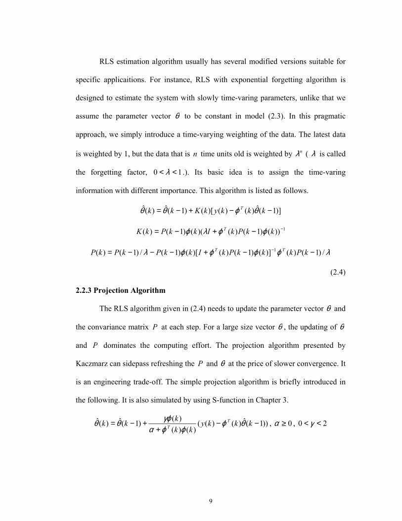
RLS estimation algorithm usually has several modified versions suitable for

specific applicaitions. For instance, RLS with exponential forgetting algorithm is

designed to estimate the system with slowly time-varing parameters, unlike that we

assume the parameter vector θ to be constant in model (2.3). In this pragmatic

approach, we simply introduce a time-varying weighting of the data. The latest data

is weighted by 1, but the data that is n time units old is weighted by ( nλ λ is called

the forgetting factor, 1<0 < λ .). Its basic idea is to assign the time-varing

information with different importance. This algorithm is listed as follows.

)]1(ˆ)()()[()1(ˆ)(ˆ −−+−= kkkykKkk T θϕθθ

1))()1()()(()1()( −−+−= kkPkIkkPkK T ϕϕλϕ

λϕϕϕϕλ /)1()()]()1()()[()1(/)1()( 1 −−+−−−= − kPkkkPkIkkPkPkP TT

(2.4)

2.2.3 Projection Algorithm

The RLS algorithm given in (2.4) needs to update the parameter vector θ and

the convariance matrix P at each step. For a large size vector θ , the updating of θ

and P dominates the computing effort. The projection algorithm presented by

Kaczmarz can sidepass refreshing the P and θ at the price of slower convergence. It

is an engineering trade-off. The simple projection algorithm is briefly introduced in

the following. It is also simulated by using S-function in Chapter 3.

))1(ˆ)()(()()(

)()1(ˆ)(ˆ −−+

+−= kkkykk

kkk TT θϕ

ϕϕαγϕθθ , 0≥α , 20 << γ

9

2.3 Control Algorithm

2.3.1 A Linear Controller of General Structure

The process model is described in (2.1) as

))()()(()()( 0011 dtvdtuzBtyzA −+−= −−

Assume that the polynomials and are co-prime, i.e. they do not have

any common factors. Furthermore, is monic. That is, that the coefficient of

the highest power is unity.

)( 1−zA

A

)( 1−zB

)( 1−z

A general linear controller can be described by

)()()()()()( 111 tyzStuzTtuzR c−−− −= (2.5)

where ) , and T are polynomials in the back shift operator .

This controller consists of a feedforward with the transfer operator

)( 1−zR ( 1−zS )( 1−z 1−z

)()(

1

1

−

−

zRzT and a

feedback with the transfer operator )()(

1

1

−

−

zRzS . It thus has two degrees of freedom. A

block diagram of the closed-loop system is illustrated in the following figure 3.

)()()()()()( 111 tyzStuzTtuzR c−−− −=

)()(

1

1

−

−

zAzB

u

v

ycuProcess Controller

Figure 3: A General Linear Controller with Two Degrees of Freedom

10

From equations (2.2) and (2.5), we can obtain the following equations for the closed-

loop system.

)()()()()(

)()()()()()()(

)()()( tvzSzBzRzA

zRzBtuzSzBzRzA

zTzBty c ++

+= (2.6)

)()()()()(

)()()()()()()(

)()()( tvzSzBzRzA

zSzBtuzSzBzRzA

zTzAtu c +−

+= (2.7)

Thus, the closed-loop characteristic polynomial is (for simplicity, the operator is

omitted)

z

BSARAc += (2.8)

The key idea of the controller design is to specify the desired closed-loop

characteristic polynomial as a design parameter. By solving the Diophantine

equation (2.8), the polynomials

cA

R and can be obtained. The closed-loop

characteristic polynomial fundamentally determines the property and the

performance of the closed system. The Diophantine equation (2.8) always has

solutions if the polynomial and

S

cA

A B are co-prime as required. And the solution may

be poorly conditioned if the polynomials have factors that are very close. The

method to solve the Diophantine equation is presented in the Appendix.

2.3.2 Model Following

The Diophantine equation (2.8) determines only the polynomials R and .

Other conditions must be introduced to calculate the polynomial

S

T in the controller

(2.5). To do this, we require that the response from the command signal to the output

follow the model

11

)()( tuBtyA cmmm = (2.9)

From equation (2.6), the following condition

m

m

c AB

ABT

BSARBT ==+

(2.10)

must hold. It then follows from the model-following condition (2.10) that the

response of the closed-loop system to command signal is as specified by the model

(2.9).

Based on the model-following condition, some constructive conclusions can

be deduced. Equation (2.10) implies that there are cancellations of factors of BT and

. Factorize the polynomial cA B as

−+= BBB (2.11)

where +B is a monic polynomial whose zeros are stable and so well damped that

they can be canceled by the controller and −B corresponds to the unstable or poorly

damped factors that cannot be canceled. Since −B remains unchanged, it thus holds

that −B must be a factor of . Therefore mB

'mm BBB −= (2.12)

Since +B is canceled, it must be a factor of . Furthermore, it follows from

equation (2.10) that, is also a factor of . The closed-loop characteristic

polynomial thus can be rewritten as

cA

cAmA

cA

omc AABA += (2.13)

12

Since and cA B have the common factor +B , it follows form equation (2.8) that it

must be also a factor of R . Hence

'RBR += (2.14)

The Diophantine equation (2.8) then can be simplified as

''com AAASBAR ==+ − (2.15)

Substituting equation (2.11), (2.12) and (2.13) into equation (2.10), there holds

om ABT '= (2.16)

2.3.3 Compatibility Condition

To have a control law that is causal in the discrete-time case, we must impose

the following conditions upon the polynomials in the control law (2.5).

RS degdeg ≤ (2.17)

RT degdeg ≤ (2.18)

In the case of no constraints on the degree of the polynomial, the Diophantine

equation (2.8) has many solutions because if *R and are two specific solutions,

then so are

*S

MBRR += * (2.19)

MASS −= * (2.20)

where M is an arbitrary polynomial with any degree. Since there are so many

solutions, it is desirable to seek the solution that gives a controller with the lowest

degree, i.e. the minimum-degree controller. Given deg , it then follows

from equation (2.8) that

BA deg>

13

AAR c degdegdeg −= (2.21)

From equation (2.20), we can always find a solution in which the degree of S is at

most . This is defined as the minimum-degree solution to the Diophantine

equation (2.8). The condition thus implies that

1deg −A

RS degdeg ≤

1deg2deg −≥ AAc (2.22)

From equation (2.16), the condition implies that RT degdeg ≤

0degdegdegdeg dBABA mm =−≥− (2.23)

It implies that the time delay of the model must be at least as large as the time delay

of the process. It is natural that to get a solution in which the controller has the

lowest possible degree. Meanwhile it is reasonable to require that there is no extra

delay in the controller. It means that the polynomials R , and S T have the same

degrees. Then, we have the following algorithm.

Minimum-degreee Pole Placement (MDPP)

Data: Polynomials and A B .

Specification: Polynomials , and . mA mB oA

Compatibility Conditions:

deg AAm deg=

deg BBm deg=

deg 1degdeg −−= +BAAo

'mm BBB −=

Step 1: Decompose B as −+= BBB

14

Step 2: Solve the diophantine equation below to get 'R and with

.

S

AS degdeg <

mo AASBAR =+ −'

Step 3: From 'RBR += and T , and compute the control signal from '0 mBA=

the control law

SyTuRu c −=

In this theis, we only consider one special case where no zeros are canceled.

Then we have 1=+B , BB =− , and BBm β= ,where )1(/)1( BAm=β , and

, T1degdeg −= AAo oAβ= . The Diophantine equation in Step 2 becomes

moc AAABSAR ==+

15

CHAPTER 3 SIMULATION OF ADAPTIVE CONTROL SYSTEMS

In this chapter, we simulate the RLS estimator algorithm and the MDPP

controller algorithm by developing the S-function code in MATLAB. S-function is a

powerful tool which enables us to add our customrized algorithm block into the

Simulink models. We will discuss what the S-function is and how to code with it.

We will also give a couple of simulation models for the adaptive control systems by

using the S-function later on.

3.1 Introduction to S-function

3.1.1 What Is an S-function

When we create a Simulink model by drawing a block diagram, an S-function

is generated with the same name as the model by the Simulink automatically and

internally. This S-function is the agent Simulink interacting with for simulation and

analysis. Though it is hidden from view, we can call it from the command line like

any other MATLAB function. We can sidestep this process by writing an S-function

by ourselves. S-functions can be written using MATLAB or C. C language S-

functions are compiled as MEX-files (MATLAB Executable files) using the mex

utility described in the Application Program Interface Guide.

In most basic sense, S-functions are simply MATLAB functions using a

special calling syntax that enables us to interact with Simulink’s equation solvers.

This interaction is very similar to the interaction that takes place between the solvers

and built-in Simulink blocks. The form of an S-function is very general and can

16

accommodate continuous, discrete, and hybrid systems. As a result, nearly all

Simulink models can be described by S-functions. S-functions are incorporated into

Simulink models by using the S-Function block in the Nonlinear Block sublibrary.

We can use the S-Function block’s dialog box to specify the name of the underlying

S-function, as illustrated in the figure 4.

3.1.2 When to Use an S-function

The most common use of S-functions is to create custom Simulink blocks.

We can use S-functions for a variety of applications, including:

• Adding new general purpose blocks to Simulink

• Incorporating existing C code into a simulation

• Describing a system as a mathematical set of equations

• Using graphical animations (see the inverted pendulum demo, penddemo)

An advantage of using S-functions is that we can build a general purpose block that

we can use many times in a model, varying parameters with each instance of the

block and integrating with our own analysis and simulation routines.

3.1.3 How S-functions Work

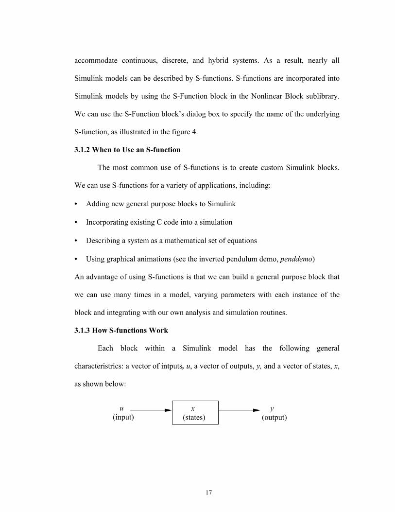
Each block within a Simulink model has the following general

characteristrics: a vector of intputs, u, a vector of outputs, y, and a vector of states, x,

as shown below:

y (output)

u (input)

x (states)

17

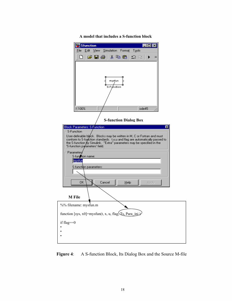
M File

S-function Dialog Box

A model that includes a S-function block

%% filename: mysfun.m function [sys, x0]=mysfun(t, x, u, flag, Ts, Para_ini ) if flag==0 • • •

Figure 4: A S-function Block, Its Dialog Box and the Source M-file

18

The state vector may consist of continuous states, discrete states, or a combination of

both. The mathematical relationships between the inputs, outputs, and the states are

expressed by the following equations:

),,( uxtfy o= (output)

),,( uxtfx dc =& (derivative)

),,(1

uxtfx udk=

+ (update)

where dc xxx +=

In M-file S-functions, Simulink partitions the state vector into two parts: the

continuous states and the dircrete states. The continuous states occupy the first part

of the state vector, and the discrete states occupy the second part. For blocks with no

states, x is an empty vector. In MEX-file S-functions, there are two separate state

vectors for the contnuous and discrete states.

Simulink makes repeated calls during specific stages of simulation to each

block in the model, directing it to perform tasks such as computing its outputs,

updating its discrete states, or computing its derivatives. Additional calls are made at

the beginning and end of a simulation to perform initialization and termination tasks.

The figure 5 illustrates how Simulink performs a simulation. First, Simulink

initializes the model; this includes initializing each block, and each S-functions.

Then Simulink enters the simulation loop, where each pass through the loop is

referred to as a simulation step. During each simulation step, Simulink executes the

S-function block. This continues until the simulation is complete. Simulink makes

repeated calls to S-functions in the model. During these calls, Simulink calls S-

19

function routines (also called methods), which perform tasks required at each stage.

These tasks include:

• Initialization — Prior to the first simulation loop, Simulink initializes the S-

function. During this stage, Simulink:

⇒

⇒

⇒

⇒

Initializes the SimStruct, a simulation structure that contains information about

the S-function.

Sets the number and size of input and output ports.

Sets the block sample time(s).

Allocates storage areas and the sizes array.

• Calculation of next sample hit — If a variable step integration routine is selected,

this stage calculates the time of the next variable hit, that is, it calculates the next

stepsize.

• Calculation of outputs in the major time step — After this call is complete, all the

output ports of the blocks are valid for the current time step.

• Update discrete states in the major time step —In this call, all blocks should

perform once-per-time-step activities such as updating discrete states for next

time around the simulation loop.

• Integration — This applies to models with continuous states and/or nonsampled

zero crossings. If your S-function has continuous states, Simulink calls the output

and derivative portions of your S-function at minor time steps. This is so

Simulink can compute the state(s) for your S-function. If your S-function (C

MEX only) has nonsampled zero crossings, then Simulink will call the output

20

and zero crossings portion of your S-function at minor time steps, so that it can

locate the zero crossings.

Figure 5: How Simulink Performs Simulation

21

3.1.4 A Simple Example of S-function

Consider a single-input, two-output set of state-space equations

BuAxx +=&

DuCxy +=

where

−−

−=

03.203.262.09.2

003.0A ; ; ; ;

=

001

B

−

=131011

C

=

10

D

=

111

0x

This can be represented both as an Simulink model including an state-space block

and a model including an S-function block, repectively in the next figure.

Figure 6: 2 Equivalent Simulink Models

22

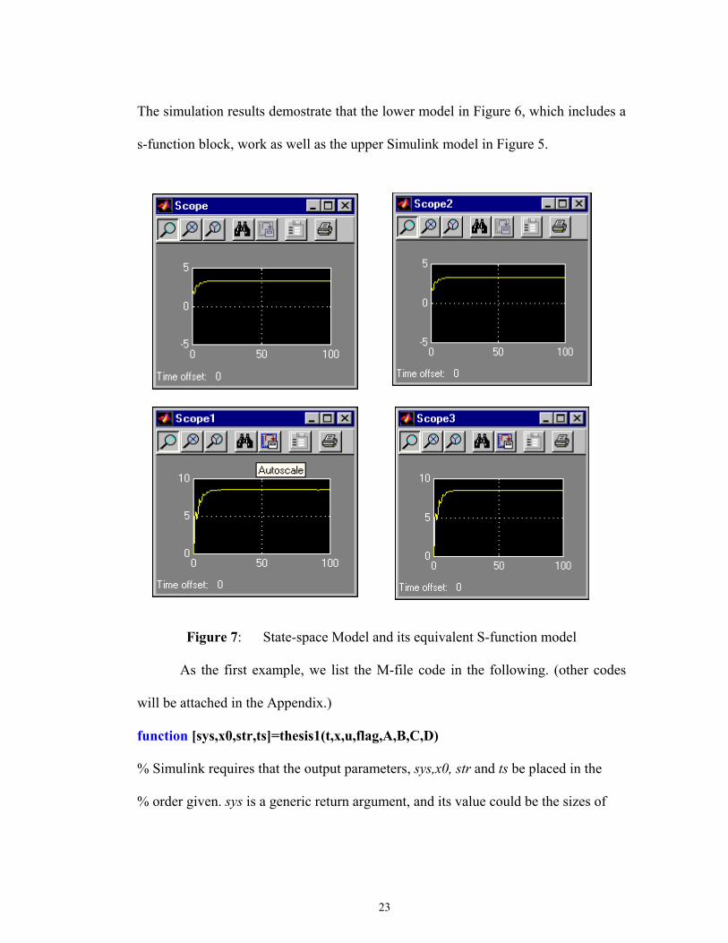
The simulation results demostrate that the lower model in Figure 6, which includes a

s-function block, work as well as the upper Simulink model in Figure 5.

Figure 7: State-space Model and its equivalent S-function model

As the first example, we list the M-file code in the following. (other codes

will be attached in the Appendix.)

function [sys,x0,str,ts]=thesis1(t,x,u,flag,A,B,C,D)

% Simulink requires that the output parameters, sys,x0, str and ts be placed in the

% order given. sys is a generic return argument, and its value could be the sizes of

23

% parameters, the state derivatives or the S-function output, depending on the flag

% options. For example, for flag=3, sys contains the S-function outputs.

% x0 is the initial state value (an empty vector if there are no states in the system). x0

% is neglected, except when flag=0.

% str is reserved for future use. S-functions must set this to the empty matrix, [].

% ts is a two column matrix containing the sample times and offsets of the block.

% thesis1 is the S-function name.

% The first four inputs parameters, which Simulink passes to the S-function, must be

% the variables t, x, u and flag. t, x and u are the current time, current state vector

% and current input vector respectively. flag is the parameter that controls the

% S-function routines at each simulation stage.

% A, B, C and D are the additional input parameters of the S-function. They could be

% inputted in the dialog box of S-function block as shown in Figure 3.

switch flag,

% flag could have value of 0, 1, 2, 3, 4, and 9. Different values determine distinct

% routines of S-function at each simulation stage. The flag options available in

% Simulink are listed in the table 1.

case 0

[m,n]=size(D);

% m is the number of outputs, n is the number of inputs;

sys=[length(A),0,m,n,0,any(D~=0)];

% For a flag=0 call, sys contains the following information vital to simulation.

24

S-function Routine Description

flag=1 Calculates the derivatives of the continuous state variables.

flag=2 Updates discrete states.

flag=3 Calculates the outputs of the S-function.

flag=4 Calculates the next sample hit for a discrete update.

flag=9 Performs any necessary end of simulation tasks.

Table 1: S-function Routines and Descriptions

sys(1) Number of Continuous States.

sys(2) Number of Discrete States.

sys(3) Number of Inputs.

sys(4) Number of Outputs.

sys(5) Number of Sample times.

sys(6) Flag for direct feedthrough.

x0=[1;1;1];

% The initial state value.

case 1

sys=A*x+B*u;

% Return the states derivatives, xDOT.

case 3

sys=C*x+D*u;

% Return system output, y.

25

otherwise

sys=[];

% In this example, no need to return anything, since this is a continuous system. It

% does not apply to other cases.

end

3.2 Simulation of RLS Estimator

The RLS estimator presented in Section 2.2.2 is simulated by using S-

function under Simulink here. We include an S-function block defined by an M-file

S-function code into an Simulink model, and excite the plant to be estimated with 1

Hz square wave. A couple of typical examples illustrate how we program the code

and set up the additional input parameters of the S-function in the dialog box, and

demonstrate the validity of the RLS estimation algorithm.

3.2.1 Plant Model and Estimation Algorithm

The plant to be estimated is in the general form as below

)()()( 1

11

−

−−− =

zDzNzzG

d

p (3.1)

where

d is the time delay, n . dm +≥

, deg[ . mm zzzN −−− +++= βββ K1

101 )( mzN =− )]( 1

, deg[ nn zzzD −−− +++= αα K1

11 1)( nzD =− )]( 1

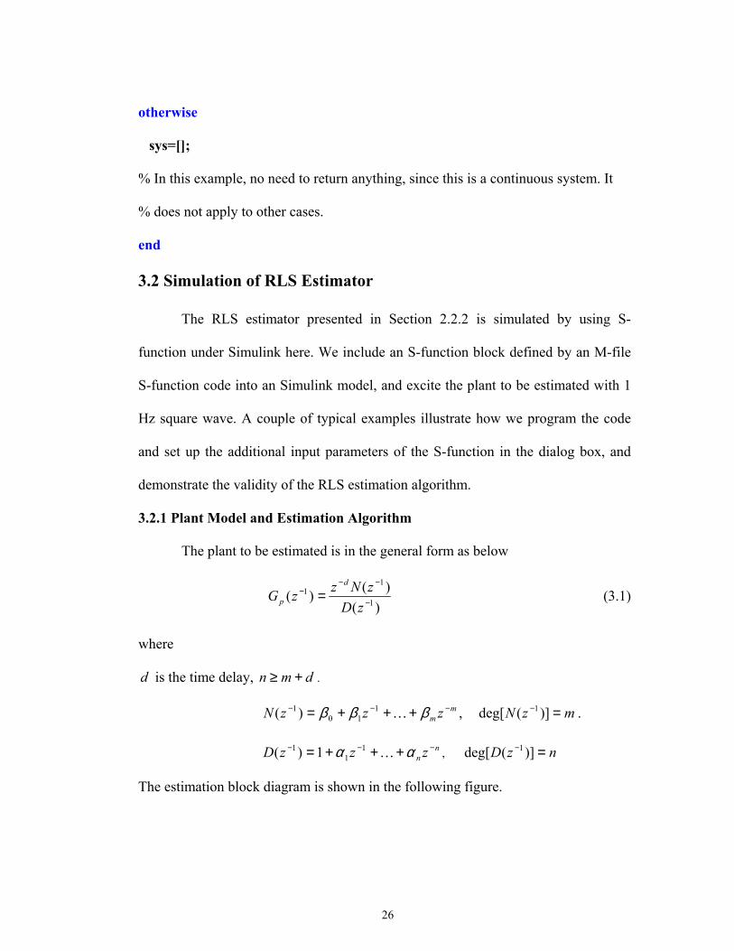
The estimation block diagram is shown in the following figure.

26

dz −n

n

mm

zzzz−−

−−

++++++ααβββ

L

L1

1

110

1

Estimator

)(ku )( dku −

Plant

)(ky

Figure 8: Estimation Block Diagram

Assuming that u and are the input and the output of the plant, respectively

we can write the plant model as below

)(k )(ky

)()1()()()( 10 nkykymdkudkuky nm −−−−−−−++−= ααββ LL (3.2)

or in the form of vector

)()()( kkky T θϕ= (3.3)

where

1)1()](),2(),1(),(),1(),([)( ×++∈−−−−−−−−−−−= mnT Rnkykykymdkudkudkuk LLϕ

1)1(2110 ],,,,,[)( ×++∈= mnT

nm Rk αααβββθ LL

The estimation algorithm is the same as the estimator presented in section 2.2.2.

)]1(ˆ)()()[()1(ˆ)(ˆ −−+−= kkkykKkk T θϕθθ

1))()1()()(()1()( −−+−= kkPkIkkPkK T ϕϕϕ

)1()()]()1()()[()1()1()( 1 −−+−−−= − kPkkkPkIkkPkPkP T ϕϕϕϕ

3.2.2 Simulation Experiments

In simulation, we use a data structure of matrix form as shown below.

(Referring to the MATLAB code in Appendix.)

27

28

Only three parameters d , m and n are needed to estimate the unknown parameters.

1. 6065.06065.1

0902.01065.0)( 2 +−+=zz

zzGp ;

)(zGp could be rewritten as 21

111

6065.06065.110902.01065.0)()( −−

−−−

+−+==

zzzzzGzG pp . Then

1=d , 1=m and 2=n . As the first example in this section, we show the Simulink

block diagram in Figure 9, the S-function dialog box in Figure 10 and the experiment

results displayed in the scopes of Figure 11..

2. 43211

12.067.081.06.011)( −−−−

−

−+−−=

zzzzzGp

It is easy to see that 0=d , 0=m and 4=n . Totally 5 unknown parameters need to

be estimated.

Parameters 0β 1α 2α 3α 4α

True Value 1 -0.6 -0.81 0.67 -0.12

Time=3s 1 -0.6 -0.81 0.67 -0.12

−−

−−−−

−−−

++++++

++

++

)2()()()(

)1()()()(

)1()()()()()()()(

)1)(1(1)1(

1

)1(2211

)1(1110

tytptpt

tytmdtut

dtutptptdtutptpt

mnmnmnn

m

mn

mn

L

MMOMM

MOM

MOM

MMOMM

L

L

α

αβ

ββ

( )tθ ( )P t ( )tϕ

)0(θ̂ 0P

1=m

2=n

M-file S-function code is attached in the Appendix

Initial Value Initial ValueTs=1s

Figure 9: S-function Dialog Box of Example 1

Figure 10: Simulink Block Diagram of Example 1

29

Figure 11: Simulation Results of Example

3. 445.009.01.1

27.02.1)( 23

2

++−++=

zzzzzzpG ;

)(zGp could be rewritten as 321

2111

445.009.01.1127.02.11)()( −−−

−−−−

++−++==

zzzzzzzGz pp

3=

G .

It holds that d , and n . Totally 6 unknown parameters need to be

estimated.

1= 2=m

30

Parameters 0β 1β 2β 1α 2α 3α

True Value 1 1.2 0.27 -1.1 0.09 0.445

Time=50s 1 1.991 0.2694 -1.1009 0.0915 0.4442

Time=500s 1 1.991 0.2694 -1.1009 0.0915 0.4442

4. 3679.03679.1

2642.03769.0)( 2 +−+=zz

zzpG

)(zGp could be rewritten as 21

111

3679.03679.112649.03679.0)()( −−

−−−

+−+==

zzzzzGz pp

1 2=

G .

Similarly we find that , and n and totally 4 unknown parameters

need to be estimated. In this example, however, we use the projection algorithm to

estimate the parameters.

1=d =m

Parameters 0β 1β 1α 2α

True Value 0.3679 0.2642 -1.3679 0.3679

Time=100s 0.3678 0.2675 -1.3645 0.3645

Time=500s 0.3678 0.2675 -1.3648 0.3648

31

3.3 Simulation of MDPP Controller

The MDPP control law presented in 2.3.4 is simulated by using S-function

under the Simulink in this section. We program 3 S-functions in M-file to estimate

the unknow process parameters, to calculate the controller parameters and to

implement the control law. The S-functions are programed in an open way so that it

applies to a general process model. Given the degree of the polynomials of the

process model and the reference model parameters, the system will be simulated

automatically. We only need pay attention to the selection of some intial values of

the unknown parameters. A second order and third order process are chosen to

illustrate the simulation procedure. The method to solve the Diophantine equation is

also discussed.

3.3.1 Simulation Steps

Data: Give the reference model in the form of a desired closed-loop pulse transfer

operator and a desired polynomial . mm AB / oA

Step 1: Estimate the coefficients of the polynomials and A B in equation (2.1) using

the RLS method given in 2.2.2.

Step 2: Using the polynomials and A B estimated in step 1, apply the MDPP

method presented in 2.3.4 . The polynomials R , and S T of the controller are then

obtained by solving the Diophantine equation (2.7).

Step 3: Compute the control action from equation (2.4), that is

)()()( tSytTutRu c −=

Repeat steps and 3 at each sampling period.

32

3.3.2 Solving the Diophantine Equation with Euclid's Algorithm

In order to compute the control law, we need to solve the following

Diophantine equation

cABSAR =+ (3.4)

The equation is linear in the polynomial of R and . A solution to the equation

existes if and

S

A B are coprime. However, the equation has many solutions. For

example, assuming that *R and are solutions, then and

are also solutions, where W is an arbitrary polynomial. A specified

solution can be achieved by imposing some constraints on the general solutions.

Since a controller must be causal, the constraint condition must hold.

The condition will restrict the number of solutions significantly. Here, we adopt

Euclid's algorithm to solve the equation.

*S BWRR += *

Rdeg≤

AWSS −= *

Sdeg

This algorithm finds the greatest common divisor of two polynomials

and

D A

B . If one of the polynomials, say , is zero, then is equal to . If this is not the

case, the algorithm follows. Let and and iterate the equations

A

AA =0 BB =0

nn BA =+1

nn AB =+1 mod nB

until . The greatest common divisor is then . Similar to the case that

when and

01 =+nB

A

nBD =

B are numbers, modA B means the reminder when is divided by A

B when and A B are polynomials. Bachtracking, we find that can be expressed

as

D

33

DBYAX =+ (3.5)

where the polynomials X and Y can be found by keeping track of div in

Euclid's algorithm. This establishes the link between Euclid's algorithm and the

Diophantine equation. The extended Euclidean algorithm gives a convenient way to

determine

nA nB

X and Y as well as the minimum-degree solutions U and V to

0=+ BVAU (3.6)

we can rewrite equation and as

=

=

0D

BA

VUYX

BA

F (3.7)

The matrix can thus be viewed as the matrix, which performs row operations on

to give [ . A convenient way to find is to observe that

F

[ TBA ] ]TD 0

=

VUYXD

BA

VUYX

01001

The extended Euclidean algorithm can be expressed as follows: start with the matrix

=

1001

BA

M

If we assume that deg , then calculate Q divBA deg≥ A= B , multiply the second

row of M by Q , an subtract from the first row. Then apply the same procedure to

the second row and repeat until the following matrix is obtained.

VUYXD

0

By using the extended Euclidean algorithm it is now straightforward to solve

the Diophantine equation (3.4) . cABSAR =+

34

This is done as follows: Determine the greatest common divisor and the

associated polynomials

D

X , Y , and V using the extremed Euclidean algorithm.

To have a solution to equation (3.4), must divide . A pariticular solution is

given by

U

D cA

cXAR =* div D

cYAS =* div D

and the general solution is

WURR += *

WVSS += *

where is an arbitrary polynomial. The minimum-degree solution is obtained by

choosing W divV . This implies that modV .

W

*S−= *SS =

By equating coefficients of equal order , the Diophantine equation given by

equation (3.4) can be written as a set of linear equations:

−

−

=

−

+

−

−

−

−

12,

1,

,

11,

1

0

1

1

221

111

2312

121

1

0000

0

0100

100001

nc

nc

nnc

c

n

n

nn

nnn

nn

a

aaa

aa

s

sr

r

ba

bbaaabbaa

bbaabba

b

M

M

M

M

LL

MOOMMOOM

OO

OMOM

OMMOMM

OO

MOMO

LL

If the time delay of the plant is , then . The matrix on the left-

hand side is called the Sylverster matrix. It occurs frequently in applied mathematics.

d 0110 === −dbbb

35

It has the property that it is nonsingular if and only if the polynomials and A B do

not have any common factors.

2−.2642

2786

)4966+z

)1−3842

3.3.3 Two Simulation Examples

For the model of Example 4 in section 3.2.2 1

211

367903679.11.03769.0)( −

−−−

+−+=

zzzzzpG .

We specify the reference model as , where mm AB /

; 4966.03205.12 +−= zzAm

.02642.03769.0

4966.03205.111

10

21 =+

+−=+++

=bb

aa mmβ ;

)2642.03769.0(*2786.0 +== zBBm β ;

; 8.0+= zAo

Following the simulation steps in section 3.3.1, we solve the Diophantine

.03205.1)(8.0()2642.03769.0()3679.03679.1( 22 −+=+++− zzSzRzz

and thus obtain the polynomials R , and S T as follows

8042.0)( += zzR

3842.01173.0)( += zzS

T 2229.02786.0)( += zz

Finally, we obtain the control law

(.0)(1173.0)1(2229.0)(2786.0)1(8042.0)( −−−++−−= tytytutututu cc

The simulation process is illustrated by the following block diagram Figure 11. In

this diagram, the S-function block "estimator" estimates the process parameters, i.e.

Step 1; the S-function block "contr_calc" is to solve the Diophantine equation and to

36

get the polynomials R , and S T , i.e. Step 2; the S-function block "controller"

computes the control law.

Figure 12: Simulation Block Diagram of A Second Order System

The output of the system is shown in the following Figure 13.

Figure 13: Output of A 2-ord System

37

321

2111

445.009.01.1127.02.11)( −−−

−−−−

++−++=

zzzzzzzGp

mB /

is the model of Example 3 in section

3.2.2. We specify the reference model as , where mA

)2.0)](4.06.0()][4.06.0([ +−−+−= zjzjzAm

= 104.028.023 ++− zzz

1555.027.02.11

104.028.011)1()1(

≈++

++−==BAmβ

0420.01866.01555.0 2 ++== zzBBm β

32.04.0)8.0)(4.0( 2 −−=−+= zzzzAo

Following the simulation steps in section 3.3.1, we need to solve the Diophantine

equation

)()27.02.1()()445.009.01.1( 223 zSzzzRzzz +++++−

)104.028.0)(32.04.0( 232 ++−−−= zzzzz

and we get the polynomials R , and S T as follows

2460.06419.0)( 2 −−= zzzR

2822.06003.03419.0)( 2 +−= zzzS

0498.00622.01555.0)( 2 −−= zzzT

Finally we get the control law in the vector form as

38

−−−−−−−−

−−−

−−−−−=

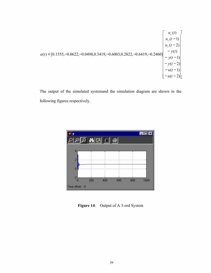
)2()1()2()1(

)()2()1(

)(

]2460.0,6419.0,2822.0,6003.0,3419.0,0498.0,0622.0,1555.0[)(

tututyty

tytutu

tu

tu

c

c

c

The output of the simulated systemand the simulation diagram are shown in the

following figures respectively.

Figure 14: Output of A 3-ord System

39

Figure 15: Simulation Block Diagram of A Third Order System

40

CHAPTER 4 ROBUSTNESS ANALYSIS AND SIMULATION

In previous sections, we mainly used S-function to implement MDPP

adaptive algorithm. And we show that adaptive control can be very useful and can

give good closed-loop performance. It is attributed to the adpative behavior of the

controller that it changes its paramtets, not the structer, according to the changing

dynmacis of the system. However, that does not mean that adaptive control is the

universal tool that should always be used. How about its robustness property? Many

papers examine the robustness of existing adaptive algorithms to unmodeled

dynamics and disturbance. The adpative controller itself is able to adjust its

parameters to the varying environments adaptively. In this sense, the adaptive

controller has the robustness to some degree. But the design guideline of adaptive

controller is extremely different from the idea of robust controller design. Charles E.

Rohrs's paper [4] robustness of continuous-time adaptive control algorithms in the

presence of unmodeled dynamics spurred much discussion in the adaptive control

community in the past years. That is the motivation for us to study the robustness in

this chapter.

4.1 Frequency Analysis of the Convergent Adaptive Controller

In this section, Bode plot technique is utilized to analyze the stability margin

of the system. We introduce unmodeled dynamics with peak value at the crossover

frequency of the system and unity magnitude in the low frequency. The simulation

41

results show that the adpative controller failes to cope with some unmodeled

dynamics.

4.1.1 Stability Margin

We choose the original plant model as

7241.00344.15.0)( 2 +−

+=zz

zzGp

This model has a pair of complex poles at 0.5172+j0.6757 and 0.5172-j0.6757 and a

zero at -0.5. It has slow response and large overshot as shown below.

In order for the feedback system to have zero tracking error for the step input, and

have zero response at high frequency, we add one more pole at 1, and one more zero

at –1. Thus, the overall plant model will be

7241.07585.10344.25.05.1)( 3

2

−+−++=

zzzzzzGp (4.1)

For this composite plant model, we use MDPP algorithm to design an adaptive

controller. The desired pole location for the closed-loop model is , 4.02.0 j+

42

4.02.0 j− , , and . This model have

better step response (shorter setting time and smaller overshoot.). It is illustrated

below.

75.0− j2069.05172.0 +− j2069.05172.0 −−

Figure 16: Step Response of Adaptive Control System

43

The adaptive control system block diagram is shown in the following figure. When

the controller parameters converge to their normal value, we obtain the following

controller from the output of the block "contr_calc_3ordT" in the Figure 17.

)()1448.04828.04667.0()()4737.04537.1( 22 tuzztuzz c++=++

− (4.2) )()7792.065.19561.1( 2 tyzz +−

Figure 17: Adaptive Control System

According to the control law (4.2), we have the equivalent controller block diagram

shown in the Figure 18.

For the convenience of analysis, we omit the feedforward part in the above figure.

Then we get the open-loop transfer function )()()()(

zRzAzSzB . By using the MATLAB

command "dbode", we can obtain the bode plot in Figure 19.

44

Figure 18: Adaptive Controller

Figure 19: Bode Plot of the Adaptive Control System

45

From Figure 19, we can find that the gain margin and the phase margin are about

5dB and 10 respectively. And the crossover frequency is around 2 rad/sec. With

such a small stability margin, the adpative control system unlikely to maintain

stability in presence of unmodeled dynamics at the crossover frequency range.

o

4.1.2 Adaptive Controller Under Unmodeled Dynamics

In order to check the robustness of the adaptive controller, we intentionally introduce

some unmodeled dynamics into the plant. We choose the plant as model (4.1)

7241.07585.10344.2

5.05.1)( 3

2

−+−++=

zzzzzzpG

and the unmodeled dynamics as

6674.01179.0

2739.08375.05.01)( 2

2

+−−+−+=

zzzzkzumG

where takes different values. k

The unmodelled dynamics can effect the control performance, even destablize the

system. The following experiments demostrate how the unmodelled dynamics

introduced make the system unstable. It implies that the adaptive control scheme has

relatively small stability margin, compared with robust control mehtods. The

adaptive behavior itself does not suffice to guarantee its stability under some

unmodelled dynamics or noise with much energy.

46

)1( ∆+ kunmodeled dynamics

Figure 20: Adaptive Controller Under Unmodeled Dynamics

1) . The unmodeled dynamics destablize the system. 5.0=k

Figure 21: System Output

47

The frequency response of the unmodeled dynamics is shown below

Figure 22: Frequency Response of Unmodeled Dynamics

2) k . The system remains stable. 48.0=

Figure 23: System Output

48

The frequency response of the unmodeled dynamics is shown below

Figure 24: Frequency Response of Unmodeled Dynamics

4) . The system is stable,too. ( in the next page) 45.0=k

Figure 25: System Output

49

The frequency response of the unmodeled dynamics is shown below.

Figure 26: Frequency Response of Unmodeled Dynamics

4.1.3 Classic Feedback Controller

Compared with the adaptive controller in the above, the following simulation

shows that classic feedback controller provides a better performance, even with a

larger size of unmodeled dynamics.

Figure 27: Feedback Controller Under Unmodeled Dynamics

50

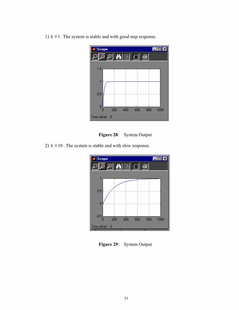
1) k . The system is stable and with good step response. 1=

Figure 28: System Output

2) k . The system is stable and with slow response. 10=

Figure 29: System Output

51

4.2 Noise Contamination

The basic idea of adaptive controller design is to estimate the plant on-line, so that

the controller can change its parameters to adapt to the changing environments.

Therefore a robust estimator in an adaptive control system plays a key role. Besides

the unmodeled dynamics introduced to the system, we also add some noise signal to

the estimator to test its estimation accuracy.

1) Adding noise to the plant output;

The magnitude of square wave from the signal generator is 1.0, and the band-limited

noise power is 0.8, the sine wave magnitude is 0.8.The block diagram is as below.

Noise Signal

Figure 30: Type 1 Noise Signal Contamination

The estimated parameters are shown in the following scopes. We can find that only

small error exist.

52

True Value is 1.0 True Value is 1.5

True Value is 0.5 True Value is –2.0344

True Value is 1.7585 True Value is –0.7241

Figure 31: Estimation Under Noise Signal (1)

53

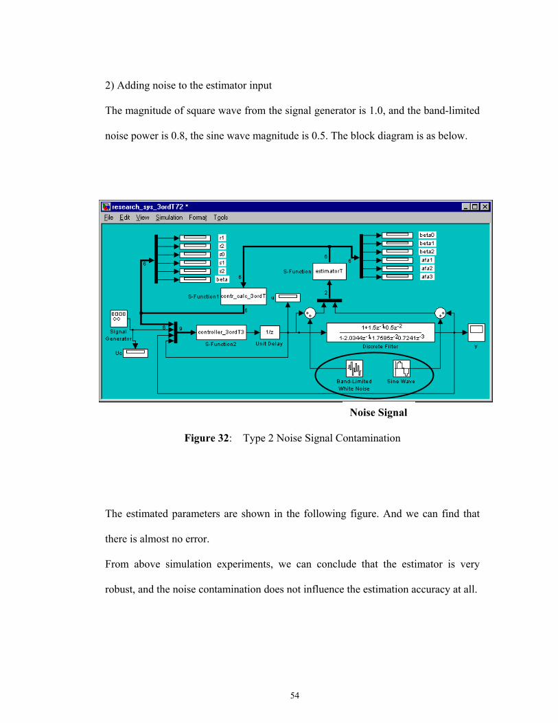
2) Adding noise to the estimator input

The magnitude of square wave from the signal generator is 1.0, and the band-limited

noise power is 0.8, the sine wave magnitude is 0.5. The block diagram is as below.

Noise Signal

Figure 32: Type 2 Noise Signal Contamination

The estimated parameters are shown in the following figure. And we can find that

there is almost no error.

From above simulation experiments, we can conclude that the estimator is very

robust, and the noise contamination does not influence the estimation accuracy at all.

54

True Value = 1.0 True Value = 1.5

True Value = 0.5True Value = –2.0344

True Value = 1.7585 True Value = –0.7241

Figure 33: Estimation Under Noise Signal (2)

55

REFERENCES

[1] K.J. strom and B. Wittenmark, "Adaptive Control", Addison-Wesley, 1995

[2] Thomas Kailath, Linear Systems, Prentice-Hall, 1980

[3] G.C. oodwin and K.S. Sin, "Adaptive Filtering, Prediction and Control", Prentice-Hall, 1984

[4] C.E. Rohrs, L. alavani, M. thans and G. tein, "Robustness of Continuous Time Adaptive Control Algorithms in the Presence of Unmodeled Dynamics", IEEE Trans. Auto. Control, Vol. 30, pp881-889, 1985

[5] P.P. Khargonekar and R.Orgeta, "Comments on the Robust Stability Analysis of Adaptive Controllers Using Normalizations", IEEE Trans. Auto. Control, Vol. 34, pp478-479, 1989

[6] L. Praly, "Robustness of Model Rreference Adaptive Control", in Proc. III Yale Workshop on Adaptive Systems, pp224-226, 1983

[7] P.A. Ioannou and K.S. Tsakalis, "A robust direct adatpive controller", IEEE Trans. Auto. Control, Vol. 31, pp1033-1043, 1986

[8] G. ao and P. oannou, "Robust Adaptive Control—A Modified Scheme", Int. J. Control, Vol. 54, pp241-256, 1992

[9] P. oannou and J. un, "Robust Adaptive Control", Prentice-Hall, 1996

[10] P. oannou and J. un, "Theory and Design of Robust Direct and Indirect Adaptive Control Schemes", Int. J. Control, Vol. 47, pp775-813, 1988

[11] D.W. Clarke, E. osca and R. attolini, "Robustness of An Adaptive Predictive Controller", IEEE Trans. Auto. Control, Vol. 39, pp1052-1056, 1994

[12] Bellman, R, "Adaptive Control----A Guided Tour", Princeton University Press, 1961

[13] Tsypkin, Y.Z, "Adaption and Learning in Automatic Systems", Academic Press, New York, 1971

56

APPENDIX SIMULATION PROGRAMS

Program 1

% filename: estimatorT.m

% this program is to estimate an unknown procee with Least-square method;

% the plant to be estimated is in the form of

% P[z^(-1)]=[z^(-d)*Num[z^(-1)]]/Den[z^(-1)];

% Num[z^(-1)]=beta_0+beta_1*z^(-1)+beta_2*z^(-2)+...+beta_m*z^(-m);

% deg(Num)=m;

% Den[z^(-1)]=1+afa_1*z^(-1)+afa_2*z^(-2)...+afa_n*z^(-n); deg(Den)=n;

function [sys,x0]=estimatorT(t,x,u,flag,ts,Para_ini,p0,m,n)

% ts=sampling time;

% Para_ini=the initial value of the parameters to be estimated;

% p0=the initial value of the convariance matrix;

% m, n=the order of Num[z^(-1)] and Den[z^(-1)], respectively;

index1=n+m+1;

% the number of the parameters to be estimated;

index2=index1^2;

% the number of the elements of P(t) matrix;

index3=index1+index2;

p1=p0*eye(index1,index1);

% the initial value of the P(t) matrix;

p2=zeros(index1,1);

57

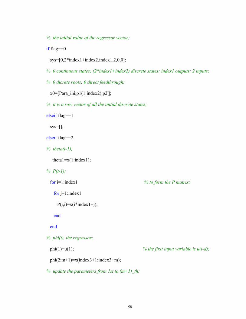
% the initial value of the regressor vector;

if flag==0

sys=[0,2*index1+index2,index1,2,0,0];

% 0 continuous states; (2*index1+index2) discrete states; index1 outputs; 2 inputs;

% 0 dicrete roots; 0 direct feedthrough;

x0=[Para_ini,p1(1:index2),p2'];

% it is a row vector of all the initial discrete states;

elseif flag==1

sys=[];

elseif flag==2

% theta(t-1);

theta1=x(1:index1);

% P(t-1);

for i=1:index1 % to form the P matrix;

for j=1:index1

P(j,i)=x(i*index1+j);

end

end

% phi(t), the regressor;

phi(1)=u(1); % the first input variable is u(t-d);

phi(2:m+1)=x(index3+1:index3+m);

% update the parameters from 1st to (m+1)_th;

58

phi(m+2:index1)=x(index3+m+2:index3+index1);

% keep parameters from (m+2)_th to index1_th unchanged;

phi=phi';

% to estimate the plant parameters with Least-square method;

temp1=P*phi;

temp2=inv(1+temp1'*phi);

P=P-temp1*temp2*temp1';

theta=theta1+P*phi*(u(2)-phi'*theta1);

% to update the phi vector;

phi(m+3:index1)=phi(m+2:index1-1);

% update parameters from (m+2)_th to index1_th;

phi(m+2)=-u(2);

% to output sys for recursive calculation;

sys=[theta',P(1:index2),phi'];

elseif flag==3

sys=x(1:index1)';

elseif flag==4

sys=ceil(t/ts+ts/1e8)*ts;

else sys=[];

end

59

Program 2

% filename: Contr_calc_3ordT.m

% this program is to calculate the 3_order controller parameters by use of STR

% algorithm;

% the reference model is represented by the s-function input parameters;

% no process zeros are canceled;

function [sys,x0]=contr_calc_3ord(t,x,u,flag,ts,para_ini,am1,am2,am3,ao1,ao2,n)

% ts=the sampling time;

% para_ini=the initial values of the controller parameters;

% am1,am2,am3,bm0,bm1,bm2=the reference model parameters;

% ao1,ao2=parameters of Ao;

% Ao=a factor of the closed-loop characteristic polynomial Ac=Ao*Am;

% n=the order of the reference model or the plant;

if flag==0

sys=[0,6,6,6,0,0];

% 0 continuous states; 6 discrete states; 6 outpus; 6 inputs;

% 0 discretes roots; 0 direct feedthrough;

x0=para_ini; % 6*1 row vector;

elseif flag==1

sys=[];

elseif flag==2

b0=u(1); b1=u(2); b2=u(3); a1=u(4); a2=u(5); a3=u(6);

60

% parameters initialization;

Coeff_B=[b0,b1,b2];

Coeff_A=[a1,a2,a3];

Coeff_AoAm=conv([1 am1 am2 am3],[1 ao1 ao2]);

%[R,S]=dio_solver(n,Coeff_A,Coeff_B,Coeff_AoAm);

[R,S]=dio_solverT(n,1,Coeff_A,Coeff_B,Coeff_AoAm(2:6));

% call a function to solve the Diophantine equations;

x(1)=R(1);

x(2)=R(2);

x(3)=S(1);

x(4)=S(2);

x(5)=S(3);

x(6)=(1+am1+am2+am3)/(b0+b1+b2); % beta

sys=x';

elseif flag==3

sys=x(1:6);

% 1st output=r1, R(z)=z^2+r1*z+r2;

% 2nd output=r2, R(z)=z^2+r1*z+r2;

% 3rd output=s0, S(z)=s0*z^2+s1*z+s2;

% 4th output=s1, S(z)=s0*z^2+s1*z+s2;

% 5th output=s2, S(z)=s0*z^2+s1*z+s2;

% 6th output=beta, T(z)=beta*Ao(z);

61

elseif flag==4

sys=ceil(t/ts+ts/1e8)*ts;

else sys=[];

end

Program 3

% filename: controller_3ordT.m;

% this program is to implement the STR algorithm;

function [sys,x0]=controller_3ordT(t,x,u,flag,ts,ao1,ao2)

% ts=the sampling time;

% ao1,ao2=parameter of Ao, Ao is a factor of the closed-loop characteristic

% polynomial Ac=Ao*Am;

if flag==0

sys=[0,5,1,9,0,6];

% 0 continuous states; 5 discrete states; 1 output; 9 inputs; 0 discrete roots; 3 direct

% feedthrough;

x0=[1,0,0,0,0];

elseif flag==1

sys=[];

elseif flag==2

xk=x(1:5);

% xk=[Uc(t),Uc(t-1),Uc(t-2),-y(t),-y(t-1),-y(t-2)-u(t-1),-u(t-2)]

62

xk(2)=xk(1); % update the xk vector;

xk(1)=u(7);

xk(4)=xk(3);

xk(3)=-u(8);

xk(5)=-u(9);

sys=xk';

elseif flag==3

xxp=[u(6)*ao1,u(6)*ao2,u(4),u(5),u(2)];

% u(6)=beta, T(z)=beta*Ao(z);

% u(5)=s2, S(z)=s0*z^2+s1*z+s2;

% u(4)=s1, S(z)=s0*z^2+s1*z+s2;

% u(3)=s0, S(z)=s0*z^2+s1*z+s2;

% u(1)=r1, R(z)=z^2+r1*z+r2;

% v u(2)=r2, R(z)=z^2+r1*z+r2;

sys=xxp*x+u(6)*u(7)-u(3)*u(8)-u(1)*u(9);

elseif flag==4

sys=ceil(t/ts+ts/1e8)*ts;

else sys=[];

end

63

Program 4

% filename: dio_solverT.m

% this program is to solve a Diophantine Equation;

% call form: [Coeff_R,Coeff_S]=dio_solverT(n,d,Coeff_A,Coeff_B,Coeff_AoAm)

% n=deg[A(z)];

% d=time delay, n-d=deg[B(z)];

% A(z)R(z)+B(z)S(z)=Ao(z)Am(z);

% A(z)=z^n+a1*z^(n-1)+a2*z^(n-2)+...+an, deg[A(z)]=n, MONIC POLYNOMIAL

% B(z)=b0*z^(n)+b1*z^(n-1)+b2*z^(n-2)+...+bn, b0=b1=b2=...=b_d-1=0,

% deg[B(z)]=n-d;

% R(z)=z^(n-1)+r_1*z^(n-2)+...+r_(n-1), deg[R(z)]=n-1, MONIC POLYNOMIAL;

% S(Z)=s_0*z^(n-1)+s_1*z^(n-2)+...+s_(n-1), deg[S(z)]=n-1 <==s_0~=0;

% Ao(z)Am(z)=z^(2n-1)+gama_1*z^(2n-2)...+gama_(2n-1)

% deg[Ao(z)Am(z)]=2n-1, MONIC POLYNOMIAL;

% Ao(z)=z^(n-1)+ao_1*z^(n-2)+...+ao_(n-1),

% deg[Ao(z)]=n-1, MONIC POLYNOMIAL;

% Am(z)=z^(n)+am_1*z^(n-1)+...+am_n, deg[Am(z)]=n, MONIC POLYNOMIAL;

% Ao(z)Am(z) can be specified by the verctor [gama_1, gama_2, ..., gama_(2n-1)]

% or by the two vectors

% [ao_1, ao_2, ..., ao_(n-1)] and [am_1, am_2, ..., am_n] respectively;

function [Coeff_R,Coeff_S]=dio_solverT(n,d,Coeff_A,Coeff_B,Coeff_AoAm)

% Coeff_A=[a1,a2,...an];

64

% Coeff_B=[b0,b1,b2,...bn];

% Coeff_AoAm=[gama_1,gama_2,...,gama_(2n-1)];

% to format the matrix M composed of the coefficients of A(z) and B(z)

% M is a (2n-1)*(2n-1) Matrix;

degA=length(Coeff_A);

degB=length(Coeff_B)-1;

if d~=(degA-degB) disp('Error in degrees of A and B!')

end

A=Coeff_A;

B=[zeros(1,d),Coeff_B]; % b0=b1=...=b_d-1=0;

Arolling=[1,A,zeros(1,n-2)];

Brolling=[B,zeros(1,n-2)];

M(:,1)=Arolling';

for i=2:n-1

M(:,i)=[0;M(1:2*n-2,i-1)];

end

M(:,n)=[Brolling(2:2*n-1),0]';

M(:,n+1)=Brolling';

for i=n+2:2*n-1

M(:,i)=[0;M(1:2*n-2,i-1)];

end

M;

65

if det(M)<1e-5

disp('A(z) and B(z) are not coprime!')

M;

end

Ac=Coeff_AoAm-[A,zeros(1,n-1)];

para=inv(M)*Ac';

Coeff_R=para(1:n-1);

Coeff_S=para(n:2*n-1);

66

VITA

Zhongshan Wu was born in China on October 21, 1974. He studied control

and systems at Northeastern University and achieved the degree of Bachelor of

Science in Eletrical Engineering on July 6, 1996. He then worked in the Research

Center of Automation at Northeastern University. He entered the master's program in

the Department of Electrical and Computer Engineering at Louisiana State

University in the spring of 2000. Now he is a candidate for the degree of Master of

Science in Electrical Engineering. In the meantime, he is studying toward a doctorate

degree in electrical engineering at Louisiana State University.

67