Simulation Studies on Effects of Dual Polarisation and ... · SIMULATION STUDIES ON EFFECTS OF DUAL...

Simulation Studies on Effects of Dual Polarisation and Directivity of Antennas on the Performance of MANETs Sharma, R. Submitted version deposited in CURVE March 2016 Original citation: Sharma, R. (2014) Simulation Studies on Effects of Dual Polarisation and Directivity of Antennas on the Performance of MANETs. Unpublished PhD Thesis. Coventry: Coventry University M. S. Ramaiah School of Advanced Studies. Copyright © and Moral Rights are retained by the author. A copy can be downloaded for personal non-commercial research or study, without prior permission or charge. This item cannot be reproduced or quoted extensively from without first obtaining permission in writing from the copyright holder(s). The content must not be changed in any way or sold commercially in any format or medium without the formal permission of the copyright holders. Some materials have been removed from this thesis due to third party copyright. Pages where material has been removed are clearly marked in the electronic version. The unabridged version of the thesis can be viewed at the Lanchester Library, Coventry University.

CURVE is the Institutional Repository for Coventry University http://curve.coventry.ac.uk/open

http://curve.coventry.ac.uk/open

Coventry University / M.S. Ramaiah School of Advanced Studies – Doctoral Programme

SIMULATION STUDIES ON EFFECTS OF

DUAL POLARISATION AND

DIRECTIVITY OF ANTENNAS ON THE

PERFORMANCE OF MANETs

Rinki Sharma

A thesis submitted in partial fulfilment

of the University’s requirements

for the Degree of Doctor of Philosophy

NOVEMBER 2014

Coventry University Research Carried out at

M. S. Ramaiah School of Advanced Studies

2

CERTIFICATE

This is to certify that the Doctoral Dissertation titled “Simulation Studies

on Effect of Dual Polarisation and Directivity of Antennas on the

Performance of MANETs”is a bonafide record of the work carried out by

Mrs. RINKI SHARMA in partial fulfilment of requirements for the

award of Doctor of Philosophy Degree of Coventry University

November-2014

Dr.Govind R .Kadambi Director of Studies M.S.Ramaiah School of Advanced Studies, Bangalore Dr. Yuri A. Vershinin Supervisor Coventry University, UK

iii

ACKNOWLEDGEMENTS

I take this opportunity to express my thanks to all those who contributed in many ways to

the success of this work. First and foremost, I thank my Director of Studies Dr. Govind R.

Kadambi for his guidance, encouragement, patience and support. He took time out of his busy

schedule for our discussions. I thank him for his time and effort to go through my thesis, and for

his valuable suggestions which helped in shaping this thesis to its present state. His dedication

towards his work is an inspiration for many.

I thank Dr. Yuri Vershinin, my CU supervisor, for his constant encouragement to publish

my work. He kept a check on the progress of my work and always responded to my mails

without any delays. He also invited me to work in laboratory at the Coventry University to work

in under his supervision.

I thank Dr. Peter White from Coventry University for visiting every year and patiently

listening to my presentations. His suggestions helped me to carry on my work in the right

direction.

I want to thank Dr. Steve Bate who was my supervisor at Coventry University. His

suggestion and inputs helped me in initial stages of my research. I thank him for spending his

time reading my long mails and giving feedback about my progress.

I am grateful to my husbandMr. Mukundan K. N. for his moral and technical support.

We had long and fruitful discussions about design, implementation and performance of the

presented work. He made many sacrifices because of my work and counselled me to carry on

when I wanted to give up. Without his support this work would not have seen the light of day.

I thank my parents Mr. O.P. Sharma and Mrs. Kusum Sharma, my brother Dr. Rahul

Sharma and my sister Mrs. Richa Sharma for teaching me to dream and work to accomplish my

dreams. I thank them for their constant love and support throughout my life. I am grateful to

them for putting up with my outbursts and still stand by me.

I express my profound gratitude to my in-laws Mr. K.S. Narasimhachar, Mrs. Suguna

B.V., Ms. S. Radhamani and Ms. K.S. Prabhamani for being cooperative during the tenure of

iv

my Ph.D. They understood my busy schedules and ensured that I am not disturbed during my

work. I thank my brother-in-law Mr. Muralikrishna K. N. for all his support during my Ph.D.

I thank my PRP committee panel members Dr. M.D. Deshpande and Prof. N.D.

Gangadhar for their valuable inputs and suggestions during the course of my work.

I thank the Vice Chancellor of M. S. Ramaiah University of Applied Sciences Dr. S. R.

Shankapal for providing us with facilities and environment that promotes research.

I take this opportunity to thank all my Colleagues, Acquaintances and Students at M. S.

Ramaiah University of Applied Sciences who directly or indirectly helped me in bringing this

work to successful completion.

I thank God for being with me all the time and walking me through this journey of life.

v

TABLE OF CONTENTS

TABLE OF CONTENTS ............................................................................................................v

LIST OF TABLES ......................................................................................................................x

LIST OF FIGURES ................................................................................................................. xii

NOMENCLATURE .................................................................................................................. xx

LIST OF ABBREVIATIONS................................................................................................ xxiii

ABSTRACT .........................................................................................................................xxvii

CHAPTER 1 ...............................................................................................................................1

1 Introduction ......................................................................................................................1

1.1 Introduction and Motivation ......................................................................................1

1.2 Research Questions ...................................................................................................6

1.3 Objectives of the Thesis.............................................................................................8

1.4 Organisation and Outline of the Thesis ......................................................................9

CHAPTER 2 ............................................................................................................................. 12

2 Mobile Ad-Hoc Networks (MANETs) ............................................................................ 12

2.1 Introduction ............................................................................................................. 12

2.2 Wireless Local Area Networks (WLANs) ................................................................ 13

2.3 Characteristics of MANETs ..................................................................................... 14

2.4 Challenges Faced by MANETs ................................................................................ 15

2.5 Physical Layer in MANETs ..................................................................................... 16

2.5.1 Received Power Computation for Free-Space and Two-Ray Ground Propagation

Models ............................................................................................................................ 17

2.5.2 Relevance of Friis’ Transmission Formula for Directional Antenna ..................... 20

2.5.3 Ranges Related to Wireless Medium .................................................................... 21

2.5.4 Types of Antenna ................................................................................................. 22

2.5.5 Antenna Characteristics ....................................................................................... 26

2.5.6 Benefits of using Directional Antenna in MANETs .............................................. 28

2.5.7 Power Control with Directional Antenna in MANETs .......................................... 30

2.5.8 Use of Dual Polarised Directional Antenna in Wireless Networks ........................ 33

2.5.9 Channel Model .................................................................................................... 37

2.6 MAC Layer in MANETs ......................................................................................... 38

vi

2.6.1 Introduction to the Hidden Node Problem ............................................................ 38

2.6.2 Survey of Methods for Handling Hidden Node Problem....................................... 39

2.6.3 IEEE 802.11 DCF Mechanism ............................................................................. 40

2.6.4 Introduction to the Exposed Node Problem .......................................................... 42

2.6.5 Directional Antenna to Reduce the Exposed Node Problem ................................. 43

2.6.6 Introduction to the Problem of Directional Exposed Node .................................... 44

2.6.7 Survey of Methods to Overcome Exposed Node Problem .................................... 44

2.6.8 Deafness due to Directional Antenna ................................................................... 48

2.6.9 Survey of Solutions to Overcome Deafness .......................................................... 49

2.6.10 MAC Layer Modifications to Incorporate Directional Antennas ........................... 52

2.7 Network Layer in MANETs .................................................................................... 53

2.7.1 Different Approaches of Routing in MANETs ..................................................... 54

2.7.2 Multipath Routing in MANETs ............................................................................ 57

2.7.3 Different Types of Multipath Routes .................................................................... 59

2.8 Vehicular Ad-Hoc Networks (VANETs) ................................................................. 62

2.9 Conclusion .............................................................................................................. 63

CHAPTER 3 ............................................................................................................................. 65

3 Mitigation of Interference through Dual Polarisation ...................................................... 65

3.1 Introduction ............................................................................................................. 65

3.2 Interference in Wireless Networks ........................................................................... 65

3.3 Use of Dual Polarised Directional Antenna to Mitigate Interference ........................ 71

3.4 Conclusion .............................................................................................................. 83

CHAPTER4 .............................................................................................................................. 84

4 Novel Scheme for Handling the Corruption of Broadcast Packets due to Hidden Terminal

Problem .................................................................................................................................... 84

4.1 Introduction ............................................................................................................. 84

4.2 Need for Handling Corruption of Broadcast Packets due to Hidden Node Problem for

Efficient Multipath Routing ................................................................................................... 84

4.3 A Novel Scheme for Handling Corruption of Broadcast Packets due to Hidden Node

Problem ................................................................................................................................ 86

vii

4.4 Simulation and Analysis of Proposed Method for Handling Corruption of Broadcast

Packets for Discovery of Neighbour Nodes ........................................................................... 97

4.5 Conclusion ............................................................................................................ 111

CHAPTER 5 ........................................................................................................................... 112

5 Avoidance of Exposed Node and Deafness using Dual Polarised Directional Antenna

based Medium Access Control (DPDA-MAC) ........................................................................ 112

5.1 Introduction ........................................................................................................... 112

5.2 Dual Polarised Directional Antenna based Medium Access Control (DPDA-MAC)

Protocol .............................................................................................................................. 112

5.2.1 Hardware Description of Antenna to Support Proposed Protocol ........................ 113

5.2.2 Sequence of Transmission of Packets in DPDA-MAC ....................................... 116

5.2.3 Flowchart for DPDA-MAC ................................................................................ 118

5.3 Avoidance of Directional Exposed Node and Deafness with DPDA-MAC ............ 128

5.4 Results and Discussion .......................................................................................... 130

5.4.1 Effect of Variation in Density and Mobility of Nodes on Throughput Achieved by

DPDA-MAC, SPDA-MAC and CSMA/CA with Varying Rate of Packet Transmission .. 134

5.4.2 Effect of Variation in Density and Mobility of Nodes on Per-Hop Delay Achieved

by DPDA-MAC, SPDA-MAC and CSMA/CA with Varying Rate of Packet Transmission ..

.......................................................................................................................... 154

5.4.3 Comparison of Performance of DPDA-MAC, SPDA-MAC and CSMA/CA with

Node Density of 100 Nodes per Unit Area ....................................................................... 172

5.4.4 Comparison of the Performance of DPDA-MAC and SPDA-MAC .................... 180

5.5 Conclusion ............................................................................................................ 183

CHAPTER 6 ........................................................................................................................... 186

6 Dual Polarised Directional Antenna based Multipath Routing Protocol (DPDA-MRP) . 186

6.1 Introduction ........................................................................................................... 186

6.2 Design of Dual Polarised Directional Antenna based Multipath Routing Protocol

(DPDA-MRP) ..................................................................................................................... 187

6.2.1 Route Discovery in DPDA-MRP........................................................................ 188

6.2.2 Route Maintenance in DPDA-MRP.................................................................... 197

viii

6.3 Formation of Routing Table and Multiple Route Discovery with Mobility of Nodes ...

.............................................................................................................................. 199

6.4 Route Disjointness in DPDA-MRP ........................................................................ 202

6.4.1 Communication over Link and Node Disjoint Routes ......................................... 205

6.4.2 Communication over Routes with Common Node .............................................. 207

6.4.3 Communication over Routes with Common Link ............................................... 209

6.4.4 Communication over Orthogonal Polarisation with Common Nodes and Links .. 210

6.5 Conclusion ............................................................................................................ 211

CHAPTER 7 ........................................................................................................................... 213

7 Performance Analysis of DPDA-MRP, SPDA-MRP and DSR ...................................... 213

7.1 Introduction ........................................................................................................... 213

7.2 Effect of Variation in Density and Mobility of Nodes on PDR Achieved by DPDA-

MRP, SPDA-MRP and DSR with Varying Rate of Packet Transmission ............................. 216

7.2.1 Analysis of Variation in PDR of DPDA-MRP .................................................... 216

7.2.2 Analysis of Variation in PDR of SPDA-MRP .................................................... 223

7.2.3 Analysis of Variation in PDR of DSR ................................................................ 229

7.3 Effect of Variation in Density and Mobility of Nodes on Throughput Achieved by

DPDA-MRP, SPDA-MRP and DSR with Varying Rate of Packet Transmission ................. 235

7.3.1 Analysis of Variation in Throughput of DPDA-MRP ......................................... 236

7.3.2 Analysis of Variation in Throughput of SPDA-MRP .......................................... 243

7.3.3 Analysis of Variation in Throughput of DSR...................................................... 250

7.4 Comparison of PDR Achieved with DPDA-MRP, SPDA-MRP and DSR with Node

Density of 100 Nodes per Unit Area .................................................................................... 255

7.5 Comparison of Throughput Achieved with DPDA-MRP, SPDA-MRP and DSR with

Node Density of 100 Nodes per Unit Area........................................................................... 259

7.6 Comparison of Throughput Achieved by DPDA-MRP and SPDA-MRP ................ 262

7.7 Conclusion ............................................................................................................ 264

CHAPTER 8 ........................................................................................................................... 266

8 Conclusions and Future Work ....................................................................................... 266

8.1 Introduction ........................................................................................................... 266

8.2 Summary ............................................................................................................... 266

ix

8.3 Conclusion ............................................................................................................ 267

8.3.1 Physical Layer ................................................................................................... 268

8.3.2 MAC Layer ........................................................................................................ 269

8.3.3 Network Layer ................................................................................................... 271

8.4 Suggestions for Future Work ................................................................................. 272

8.4.1 Suggestions for Improvement in Physical Layer ................................................. 273

8.4.2 Suggestions for Improvement in MAC layer ...................................................... 274

8.4.3 Suggestions for Improvement in Network Layer ................................................ 274

REFERENCES ....................................................................................................................... 276

APPENDIX 1.......................................................................................................................... 296

A1.1 Introduction ........................................................................................................... 296

A1.2 Simulators Considered for Implementation and Their Limitations ......................... 296

A1.3 Details of the Developed Simulation Tool ............................................................. 298

A1.4 Packet Exchange and Processing ........................................................................... 302

A1.5 Architecture of the Developed Simulation Tool ..................................................... 305

A1.6 Validation of the Developed Simulation Tool ........................................................ 306

APPENDIX 2.......................................................................................................................... 311

APPENDIX 3.......................................................................................................................... 312

x

LIST OF TABLES

Table 3-1 Scenario Specification to Study Interference .............................................................. 67

Table 3-2 Beam Orientation of Transmitting and Receiving Nodes in 32 Nodes Scenario ......... 75

Table 3-3 Scenario Specification for Dual Polarised Communication ........................................ 76

Table 4-1 Example of Neighbour Table ..................................................................................... 87

Table 4-2 Scenario Specifications to Study Performance of Broadcast Corruption Handling

Scheme ..................................................................................................................................... 99

Table 4-3 Standard Deviation with respect to Mean for Number of Nodes Missed during Node

Discovery ................................................................................................................................ 106

Table 4-4 Standard Deviation with respect to Mean for Total Time Taken for Neighbour Node

Discovery ................................................................................................................................ 110

Table 5-1 Timeout Values for Different Frames ...................................................................... 127

Table 5-2Scenario Specifications for Performance Analysis of MAC Protocols ....................... 133

Table 5-3 Standard Deviation with respect to Mean for DPDA-MAC Throughput ................... 139

Table 5-4 Standard Deviation with respect to Mean for SPDA-MAC Throughput ................... 146

Table 5-5 Standard Deviation with respect to Mean for CSMA/CA Throughput ...................... 152

Table 5-6 Standard Deviation with respect to Mean for DPDA-MAC Per-Hop Delay ............. 159

Table 5-7 Standard Deviation with respect to Mean for SPDA-MAC Per-Hop Delay .............. 165

Table 5-8 Standard Deviation with respect to Mean for CSMA/CA Per-Hop Delay ................. 171

Table 6-1 Scenario Specifications for Simulations to Analyse Route Discovery and RT

Formation with DPDA-MRP ................................................................................................... 200

Table 6-2 Routing Table Entries at Node 0 for Nodes 8 and 2 at 80ms .................................... 202

Table 6-3 Routing Table Entries at Node 0 for Nodes 8 and 2 at 660ms .................................. 202

Table 6-4 Scenario Specifications for Simulations Carried out to Study Disjointness of Routes

............................................................................................................................................... 205

Table 7-1 Scenario Specifications for Simulations to Study the Performance of DPDA-MRP,

SPDA-MRP and DSR ............................................................................................................. 215

Table 7-2 Standard Deviation with respect to Mean for DPDA-MRP PDR .............................. 222

Table 7-3 Standard Deviation with respect to Mean for SPDA-MRP PDR .............................. 228

Table 7-4 Standard Deviation with respect to Mean for DSR PDR .......................................... 234

Table 7-5 Standard Deviation with respect to Mean for DPDA-MRP Throughput ................... 241

xi

Table 7-6 Standard Deviation with respect to Mean for SPDA-MRP Throughput .................... 248

Table 7-7 Standard Deviation with respect to Mean for DSR Throughput ................................ 254

xii

LIST OF FIGURES

Figure 2-1 Two-Ray Ground Reflection Model ......................................................................... 19

Figure 2-2 Radiation Pattern of an Omnidirectional Antenna (Blake 2000) ............................... 23

Figure 2-3 Radiation Pattern of a Directional Antenna .............................................................. 24

Figure 2-4 Directional Antenna Beamforming and Null Steering ............................................... 25

Figure 2-5 Beams in a Switched Beam Antenna ........................................................................ 25

Figure 2-6 Steered Beam Antenna ............................................................................................. 26

Figure 2-7 Beamwidth of an Antenna (Blake 2000) ................................................................... 26

Figure 2-8 Vertical Polarisation (Chilukuri 2012) ...................................................................... 27

Figure 2-9 Horizontal Polarisation (Chilukuri 2012) .................................................................. 27

Figure 2-10 Two State Markov Channel Model ......................................................................... 37

Figure 2-11 Hidden Node Problem ............................................................................................ 38

Figure 2-12The CSMA/CA Mechanism .................................................................................... 41

Figure 2-13 Exposed Node Scenario .......................................................................................... 43

Figure 2-14 Exposed Node Avoidance using Directional Antenna ............................................. 43

Figure 2-15Exposed Node in Presence of Directional Communication ...................................... 44

Figure 2-16Scenario for Deafness ............................................................................................. 48

Figure 3-1 Scenario with Non-Interfering Nodes ....................................................................... 68

Figure 3-2 Signal at Physical Layer with Non-Interfering Nodes ............................................... 68

Figure 3-3 Number of Packets Sent and Received with Non-Interfering Nodes ......................... 69

Figure 3-4 Scenario with Interfering Nodes ............................................................................... 69

Figure 3-5 Signal at Physical Layer with Interfering Nodes ....................................................... 70

Figure 3-6 Number of Packets Sent and Received with Interfering Nodes ................................. 71

Figure 3-7 Orientation of Switched Beams in Qualnet ............................................................... 73

Figure 3-8 Directional Communication without Interference among Nodes ............................... 74

Figure 3-9 Communication among Different Transmitter-Receiver Pairs ................................... 77

Figure 3-10 Packets Sent and Received for Directional Communication of Nodes over VP when

Transmitters of First and Second Links are not in Interference Range of Each Other ................. 78

Figure 3-11 Directional Communication where Transmitter of First Link Interferes with

Transmitter of Second Link ....................................................................................................... 79

xiii

Figure 3-12 Packets Sent and Received for Directional Communication of Nodes over VP when

Transmitters of First and Second Links are Placed Within Interference Range of Each Other .... 80

Figure 3-13 Packets Sent and Received for Directional Communication of Nodes over

Orthogonal Polarisations with Transmitters of First and Second Links Placed Within Interference

Range of Each Other ................................................................................................................. 82

Figure 4-1 Flowchart to Overcome Hidden Node Problem ........................................................ 89

Figure 4-2 Flowchart to Overcome Hidden Node Problem (Continued) ..................................... 90

Figure 4-3Case 1 for Broadcast Packet Corruption due to Hidden Node Problem ...................... 91

Figure 4-4Timing Diagram for Case 1 ....................................................................................... 92





Figure 4-9 Case 4 for Broadcast Packet Corruption due to Hidden Node Problem ..................... 96

Figure 4-10 Timing Diagram for Case 4(a) ................................................................................ 96

Figure 4-11 Timing Diagram for Case 4(b) ............................................................................... 97

Figure 4-12Number of Neighbour Nodes Missed when Broadcast Packets are Transmitted at 2

Mbps ....................................................................................................................................... 103

Figure 4-13 Number of Neighbour Nodes Missed when Broadcast Packets are Transmitted at

11Mbps ................................................................................................................................... 104

Figure 4-14 Number of Neighbour Nodes Missed when Broadcast Packets are Transmitted at

54Mbps ................................................................................................................................... 105

Figure 4-15Total Time Taken for Neighbour Node Discovery for 1 Attempt ........................... 107

Figure 4-16Total Time Taken for Neighbour Node Discovery for 2 Attempts ......................... 108



Figure 4-19 Total Time Taken for Neighbour Node Discovery for 5 Attempts ........................ 110

Figure 5-1 Hardware Description of Antenna (Scheme 1) ........................................................ 113

Figure 5-2 Hardware Description of Antenna (Scheme 2) ........................................................ 114

Figure 5-3 Hardware Description of PIFA Antenna(Kadambi and Sullivan 2003) ................... 115

Figure 5-4Sequence of Packet Transmission in DPDA-MAC .................................................. 118

xiv

Figure 5-5 Flowchart of the Transmitter using DPDA-MAC ................................................... 122

Figure 5-6 Flowchart of the Transmitter using DPDA-MAC (Continued) ................................ 123

Figure 5-7Flowchart of the Receiver for DPDA-MAC ............................................................ 125

Figure 5-8Directional Exposed Node Problem Avoidance with DPDA-MAC .......................... 128

Figure 5-9Deafness Avoidance with DPDA-MAC .................................................................. 129

Figure 5-10 Variation in Throughput with Node Density at Different Values of Node Mobility

for DPDA-MAC at1 Packet per Second .................................................................................. 135


for DPDA-MAC at 5 Packets per Second ................................................................................ 136


for DPDA-MAC at 15 Packets per Second .............................................................................. 137




for SPDA-MAC at1 Packet per Second ................................................................................... 142


for SPDA-MAC at 5 Packets per Second ................................................................................. 143

Figure 5-16Variation in Throughput with Node Density at Different Values of Node Mobility for

SPDA-MAC at 15 Packets per Second .................................................................................... 144


SPDA-MAC at 25 Packets per Second .................................................................................... 145


CSMA/CA at 1 Packet per Second .......................................................................................... 149


CSMA/CA at 5 Packets per Second ......................................................................................... 150


CSMA/CA at 15 Packets per Second ....................................................................................... 151


for CSMA/CA at 25 Packets per Second ................................................................................. 152

Figure 5-22 Variation in Per-Hop Delay with Node Density at Different Values of Node Mobility

for DPDA-MAC at 1 Packet per Second .................................................................................. 155

xv


for DPDA-MAC at 5 Packets per Second ................................................................................ 156





Figure 5-26Variation in Per-Hop Delay with Node Density at Different Values of Node Mobility

for SPDA-MAC at 1 Packet per Second .................................................................................. 161


for SPDA-MAC at 5 Packets per Second ................................................................................. 162


for SPDA-MAC at 15 Packets per Second ............................................................................... 163


for SPDA-MAC at 25 Packets per Second ............................................................................... 164


for CSMA/CA at 1 Packet per Second ..................................................................................... 167


for CSMA/CA at 5 Packets per Second ................................................................................... 168





Figure 5-34 Variation in Throughput against Node Mobility for Different Rates of Packet

Transmission at 54 Mbps and 100 Nodes per Unit Area .......................................................... 173


Transmission at 11Mbps and 100 Nodes per Unit Area ........................................................... 174


Transmission at 2 Mbps and 100 Nodes per Unit Area ............................................................ 175

Figure 5-37Variation in Per-Hop Delay against Node Mobility for Different Rates of Packet


xvi





Figure 5-40 Comparison of Throughput Achieved by DPDA-MAC and SPDA-MAC for Varying

Node Density at Different Rates of Packet Transmission ......................................................... 181

Figure 6-1 Overall Flowchart for DPDA-MRP ........................................................................ 189

Figure 6-2 DPDA-MRP Route Discovery at Original Source .................................................. 191

Figure 6-3 DPDA-MRP Flowchart for Intermediate Node ....................................................... 193

Figure 6-4DPDA-MRP Flowchart for Intermediate Node (Continued) .................................... 194

Figure 6-5 Route Discovery at Ultimate Destination Nodes ..................................................... 195

Figure 6-6 FSM for Route Discovery Mechanism ................................................................... 196

Figure 6-7 Route Maintenance in DPDA-MRP ........................................................................ 198

Figure 6-8 FSM for Route Maintenance in DPDA-MRP ......................................................... 199

Figure 6-9 Initial Node Placement ........................................................................................... 201

Figure 6-10 Node-Disjoint Routes ........................................................................................... 203

Figure 6-11 Link-Disjoint Routes ............................................................................................ 203

Figure 6-12 Routes with Common Nodes using Dual Polarised Communication ..................... 204

Figure 6-13 Routes with Common Links using Dual Polarised Communication ...................... 204

Figure 6-14 Node-Disjoint and Link-Disjoint Routes .............................................................. 206

Figure 6-15 Timeline for Per Hop Exchange of Packets for Node-Disjoint and Link-Disjoint

Routes ..................................................................................................................................... 206

Figure 6-16 Simultaneous Communication over Orthogonal Polarisations for Node-Disjoint and

Link-Disjoint Routes ............................................................................................................... 207

Figure 6-17 Routes with Common Node ................................................................................. 207

Figure 6-18 Timeline for Per Hop Exchange of Packets for Routes with Common Node ......... 208

Figure 6-19 Simultaneous Communication over Orthogonal Polarisations for Routes with

Common Nodes ...................................................................................................................... 208

Figure 6-20 Communication over Common Link .................................................................... 209

Figure 6-21 Timeline for Per Hop Exchange of Packets for Common Link .............................. 209

Figure 6-22 Simultaneous Communication over Orthogonal Polarisations for Common Link .. 210

xvii

Figure 6-23 Communication over Common Nodes and Links .................................................. 210

Figure 6-24 Timeline for Per Hop Exchange of Packets over Common Nodes and Links ........ 211

Figure 6-25 Simultaneous Communication over Orthogonal Polarisations for Common Nodes

and Links ................................................................................................................................ 211

Figure 7-1 Variation in PDR with Node Density at Different Values of Node Mobility for

DPDA-MRP at1 Packet per Second ......................................................................................... 217


DPDA-MRP at 5 Packets per Second ...................................................................................... 218


DPDA-MRP at 15 Packets per Second .................................................................................... 219


DPDA-MRP at 25 Packets per Second .................................................................................... 221

Figure 7-5 Variation in PDR with Node Density at Different Values of Node Mobility for SPDA-

MRP at 1 Packet per Second ................................................................................................... 224


MRP at 5 Packets per Second .................................................................................................. 225


MRP at 15 Packets per Second ................................................................................................ 226

Figure 7-8Variation in PDR with Node Density at Different Values of Node Mobility for SPDA-

MRP at 25 Packets per Second ................................................................................................ 227

Figure 7-9 Variation in PDR with Node Density at Different Values of Node Mobility for DSR at

1 Packet per Second ................................................................................................................ 230

Figure 7-10 Variation in PDR with Node Density at Different Values of Node Mobility for DSR

at 5 Packets per Second ........................................................................................................... 231


at 15 Packets per Second ......................................................................................................... 232


at 25 Packets per Second ......................................................................................................... 233


for DPDA-MRP at1 Packet per Second ................................................................................... 237

xviii


for DPDA-MRP at 5 Packets per Second ................................................................................. 238


for DPDA-MRP at 15 Packets per Second ............................................................................... 239


for DPDA-MRP at 25 Packets per Second ............................................................................... 240


for SPDA-MRP at 1 Packet per Second ................................................................................... 243


for SPDA-MRP at 5 Packets per Second ................................................................................. 244


for SPDA-MRP at 15 Packets per Second ............................................................................... 246


for SPDA-MRP at 25 Packets per Second ............................................................................... 247


for DSR at 1 Packet per Second ............................................................................................... 250


for DSR at 5 Packets per Second ............................................................................................. 251


for DSR at 15 Packets per Second ........................................................................................... 252


for DSR at 25 Packets per Second ........................................................................................... 253

Figure 7-25 Variation in PDR against Node Mobility for Different Rates of Packet Transmission

at 54 Mbps and 100 Nodes per Unit Area ................................................................................ 256


at 11Mbps and 100 Nodes per Unit Area ................................................................................. 257


at 2 Mbps and 100 Nodes per Unit Area .................................................................................. 258

Figure 7-28Variation in Throughput against Node Mobility for Different Rates of Packet


xix

Figure 7-29Variation in Throughput against Node Mobility for Different Rates of Packet




Figure 7-31 Comparison of Throughput Achieved by DPDA-MRP and SPDA-MRP for Varying

Node Density at Different Rates of Packet Transmission ......................................................... 263

Figure A1 Top Level Implementation of the Developed Simulator .......................................... 298

Figure A2 Processing of Data Exchanged over Vertical and Horizontal Polarisations .............. 305

Figure A3 Architecture of the Developed Simulation Tool ...................................................... 305

Figure A4 Scenario with Non-Interfering Nodes ..................................................................... 306

Figure A5 Portion of Log File for Scenario with Non-Interfering Nodes ................................. 307

Figure A6 Number of Packets Transmitted with Non-Interfering Nodes .................................. 307

Figure A7 Number of Packets Transmitted with Non-Interfering Nodes .................................. 308

Figure A8 Scenario with Interfering Nodes ............................................................................. 308

Figure A 9 Portion of Log Files for Scenario with Interfering Nodes ....................................... 309

Figure A 10 Number of Packets Received with Interfering Nodes ........................................... 309

xx

NOMENCLATURE

Units

µs Microsecond

dB Decibel

dBi Decibel-isotropic

dBm Decibel-milliwatts

GHz Gigahertz

kbps Kilo bits per second

m Meter

m2 Meter square

m/s Meters per Second

Mbps Mega bits per second

ms Millisecond

s Second

W Watt

W/m2 Watt per meter square

V/m Volts per meter

sr Steradian

W ⋅ sr−1 Watt per steradian

Symbols Pr Power delivered to the receiver

Pt Transmitter power

𝑃𝑃𝑑𝑑 Power flux density

𝑑𝑑 Distance between transmitting and receiving nodes

𝑑𝑑0 Reference distance

𝑃𝑃𝑑𝑑𝑑𝑑 Power density of real antenna

𝑃𝑃𝑑𝑑𝑑𝑑 Power density of an isotropic antenna

𝑃𝑃 Radiated power

Gt Gain of transmitting antenna

Gr Gain of receiver antenna

xxi

E Electric field

𝐸𝐸𝑇𝑇𝑇𝑇𝑇𝑇 Total electric field

𝐸𝐸𝐿𝐿𝑇𝑇𝐿𝐿 Direct Line of Sight component of electric field

𝐸𝐸𝑔𝑔 Ground reflected component of electric field

Er Reflected component of electric field

Ei Incident component of electric field

𝐸𝐸0 Electric field in free space

ht Height of transmitter antenna

hr Height of receiver antenna

𝑘𝑘 Constant

𝐷𝐷𝑡𝑡 Directivity of transmitting antenna

𝐷𝐷𝑟𝑟 Directivity of receiving antenna

𝑈𝑈 Radiation intensity of an antenna

𝑈𝑈𝑜𝑜 Radiation intensity of an isotropic antenna

𝐴𝐴𝑒𝑒 Effective area of the antenna

e Efficiency of antenna

λ Signal wavelength

𝛺𝛺 Projected solid angle of an antenna

Ri Interference range

TSNR Threshold SNR

θ Antenna beamwidth beam angle, elevation

𝜙𝜙 Azimuth

° Degree

D Directivity of antenna

CWmin Minimum value of contention window time slots

CWmax Maximum value of contention window time slots

Gd Gain of directional antenna

Go Gain of omnidirectional antenna

δ Difference in transmission power

𝑃𝑃(𝑐𝑐) Power radiated in desired polarisation (co-polar signal)

xxii

𝑃𝑃(𝑥𝑥) Power transferred to the polarisation orthogonal to the desired polarisation (cross-

polar component)

𝜒𝜒 Lognormally distributed random variable

a constant with value much smaller than 1

µc Mean

π Pi

σc Standard deviation

xxiii

LIST OF ABBREVIATIONS

ACK Acknowledgement

AoA Angle of Arrival

AODV Ad-hoc On-demand Distance Vector

AODVM AODV Multipath

AOMDV Ad-hoc On demand Multipath Distance Vector

AP Access Point

BER Bit Error Rate

BMAC Beamformed Medium Access Control

BS Base Station

BT Busy Tone

BT-DMAC Busy Tone-Directional Medium Access Control

BTMA Busy Tone Multiple Access

CDP Corruption Detection Pulse

CDR-MAC Circular Directional RTS MAC

CGSR Clusterhead Gateway Switch Routing

CHAMP Caching and Multipath Routing Protocol

CPDMAC Cooperative Polarisation Directional Medium Access Control

CPR Cross-Polarisation Ratio

CRC Cyclic Redundancy Check

CRCM Circular RTS and CTS MAC

CRTS Circular RTS

CRDMAC Circular Ready To Receive Directional Medium Access Control

CSMA/CA Carrier Sense Multiple Access/Collision Avoidance

CTS Clear To Send

CW Contention Window

CWmax Maximum Contention Window

CWmin Minimum Contention Window

DBTMA Dual Busy Tone Multiple Access

DBTMA/DA Dual Busy Tone Multiple Access with Directional Antenna

DCF Distributed Coordination Function

xxiv

DCTS Directional Clear To Send

dCTS Directional CTS

DDR Distributed Dynamic Routing

DIFS Distributed Coordination Function-Inter Frame Space

DMAC Directional Medium Access Control

DMAC-NT Directional Medium Access Control using NAV Table

DMAC-PDX Directional Medium Access Control using Polarisation Diversity

Extension

DMAP Directional Medium Access Protocol

DNAV Directional Network Allocation Vector

DoA Direction of Arrival

DPDA Dual Polarised Directional Antenna

DPDA-MAC Dual Polarised Directional Antenna based Medium Access Control

DPDA-MRP Dual Polarised Directional Antenna based Multipath Routing Protocol

dRTS Directional RTS

DSDV Destination Sequenced Distance Vector

DSDMAC Dual-Sensing Directional Medium Access Control

DSR Dynamic Source Routing

DtD-MAC Directional-to-Directional Medium Access Control

DVCS Directional Virtual Carrier Sensing

DVCS Directional Virtual Carrier Sensing

EMRP Energy aware Multipath Routing Protocol

EIRP Effective Isotropic Radiated Power

FAMA Floor Acquisition Multiple Access

FAST Full-duplex Attachment System

FSM Finite State Machine

GPS Global Positioning System

HP Horizontal Polarisation

ID Identifier

IEEE Institute of Electrical and Electronics Engineers

ISM Industrial, Scientific and Medical

xxv

IFA Inverted F Antenna

LOS Line Of Sight

Link ID Link Identifier

LP Listening Phase

MAC Medium Access Control

MACA Multiple Access Collision Avoidance

MACA-BI Multiple Access Collision Avoidance- By Invitation

MACAW Multiple Access Collision Avoidance for Wireless-LANs

MANET Mobile Ad hoc Network

MIMO Multiple Input Multiple Output

NAV Network Allocation Vector

NCDMAC Nested Circular Directional Medium Access Control

NLOS Non-Line Of Sight

NT Neighbour Table

oCTS Omnidirectional CTS

OLSR Optimised Link State Routing

OTS Object To Send

oRTS Omnidirectional RTS

OPDMAC Opportunistic Directional MAC

PCD-MAC Power Controlled Directional Medium Access Control

PCF Point Coordination Function

PDR Packet Delivery Ratio

PHY Physical Layer

PH-DMAC Physical layer aware Directional Medium Access Control

PIFA Planar Inverted F Antenna

QoE Quality of Experience

QoS Quality of Service

RAD Random Assessment Delays

RERR Route Error

RI-BTMA Receiver Initiated- Busy Tone Multiple Access

RREP Route Reply

xxvi

RREQ Route Request

RSSI Received Signal Strength Indicator

RT Routing Table

RTS Request To Send

RTR Ready To Receive

SIFS Short Inter Frame Space

SIR Signal to Interference Ratio

SINR Signal to Interference and Noise Ratio

SMF Simplified Multicast Forwarding

SMR Split Multipath Routing

SNR Signal to Noise Ratio

SPDA Single Polarised Directional Antenna

SPDA-MAC Single Polarised Directional Antenna based Medium Access Control

SPDA-MRP Single Polarised Directional Antenna based Multipath Routing Protocol

STL Standard Template Library

SYN-DMAC Synchronized Directional Medium Access Control

TORA Temporally-Ordered Routing Algorithm

ToneDUDMAC Tone Dual Channel Directional Medium Access Control

ToneDMAC Tone Directional Medium Access Control

TT Token Tone

TTL Time-To-Live

VP Vertical Polarisation

Wi-Fi Wireless Fidelity

WLAN Wireless Local Area Network

ZD-MPDSR Zone-Disjoint Multi-Path Dynamic Source Routing

ZHLS Zone-based Hierarchical Link State

ZRP Zone Routing Protocol

xxvii

ABSTRACT

In the purview of efficient communication in MANETs for enhanced data rates and reliable

routing of information, this thesis deals with dual polarised directional antenna based

communication. This thesis proposes a dual polarised directional communication based cross-

layer solution to mitigate the problems of interference, exposed nodes, directional exposed

nodes, and deafness, and to achieve efficient routing of information. At the physical layer of

network protocol stack, this thesis proposes the use of dual polarised directional antenna for the

mitigation of interference. Use of dual polarised directional communication at the physical layer

calls for appropriate modifications in the functionality of MAC and network layers. At the MAC

layer, the DPDA-MAC protocol proposed in this thesis achieves mitigation of the problems of

exposed nodes, directional exposed nodes and deafness, by using dual polarised directional

antenna at physical layer. At network layer, the DPDA-MRP protocol presented in this thesis

facilitates the discovery of multiple routes between the source and destination nodes to route

information in accordance with the desired dual polarised directional communication. To achieve

efficient dual polarised directional communication and routing of information, it is essential to

maintain well populated Neighbour Table (NT) and Routing Table (RT). This thesis proposes a

novel Corruption Detection Pulse (CDP) based technique to handle corruption of broadcast

packets such as Link ID and RREQ arising due to hidden node problem. Since the nodes

participating in the formation of MANETs have limited battery energy, the protocols proposed in

this thesis are featured with a provision for dynamic power control to achieve energy efficient

communication. Nodes maintain Received Signal Strength Indicator (RSSI) information in the

NT, which along with the information of node location is used in the formulation of decision

logic of dynamic power control. Through numerous simulation studies, this thesis demonstrates

the benefits of dual polarised directional communication to enhance the performance of

MANET. The design principles, benefits and conceptual constraints of proposed DPDA-MAC

protocol are analysed with SPDA-MAC and CSMA/CA, while those for DPDA-MRP are

analysed with SPDA-MRP and DSR through performance metrics of throughput, Packet

Delivery Ratio (PDR) and per hop delay. The thesis also analyses the impact of variations of

channel capacity, node density, rate of packet transmission and mobility of nodes on the

performance of the proposed and conventional protocols invoked in MANETs.

1

CHAPTER 1

1 Introduction

1.1 Introduction and Motivation

Wireless communication has become an integral part of modern daily life as it provides ease of

communication while on the move. The ever increasing popularity of wireless communication

paved way for different standards for wireless network technologies. The most popular standard

which is followed to establish Wireless Local Area Networks (WLANs) is the IEEE 802.11

standard. The first IEEE 802.11 standard was introduced in the year 1997 (Hiertz et al. 2010).

Since then, extensive research has been pursued to enhance the data rates and throughput of these

networks to improve the Quality of Service (QoS) and Quality of Experience (QoE). According

to IEEE 802.11 standards, wireless networks can be established either as infrastructure based or

infrastructure less ad-hoc networks (Forouzan 2007). While the nodes in infrastructure based

network communicate through Access Point (AP) or Base Station (BS), in ad-hoc networks,

nodes communicate directly without using services of AP or BS (Forouzan 2007). Absence of

AP or BS allows for easy and fast deployment of ad-hoc networks. Ease of deployment without

investing in infrastructure has made ad-hoc networks popular among system developers and

users. Ad-hoc networks can also be deployed during situations of emergency such as natural

disasters to establish communication between rescue teams and among the victims to enable

communication and provide healthcare in the absence of infrastructure such as AP or BS. Mobile

Ad-hoc Networks (MANETs) are the ad-hoc networks established among mobile nodes where

nodes can move within an area and keep communicating with other nodes (possibly mobile) in

the same network. Due to the absence of AP or BS, the task of routing of information rests with

the nodes that form the network. In MANETs, all the participating nodes act as source, sink or

router of information (Macker and Corson 2004). All the nodes maintain routing tables to

support multihop communication between source and destination nodes which may not be

located within the direct communication range of each other. However, routes may break due to

mobility of nodes. Multihop communication can also lead to drop in throughput of a wireless

network, as noted in (Li et al. 2001).Interference is another cause for degradation in performance

of wireless networks (Jain et al. 2005)and (Padhye et al. 2005).

2

IEEE 802.11 based ad-hoc networks mainly use omnidirectional antenna for communication

(Gossain et al. 2005) and (Kumar, Arunan and Balakrishnan 2003). Use of omnidirectional

antenna leads to interference among nodes communicating over wireless medium due to lack of

provision for spatial reuse. The packets exchanged by nodes over the wireless network are prone

to corruption due to the problem of hidden nodes (Kumar, Arunan and Balakrishnan 2003). To

avoid this, the IEEE 802.11 standard uses Carrier Sense Multiple Access/Collision Avoidance

(CSMA/CA) technique to access the wireless medium (IEEE LAN/MAN Standards Committee

1999). However, the CSMA/CA mechanism leads to the problem of exposed nodes due to

omnidirectional communication (Shukla, Chandran-Wadia and Iyer 2003). To overcome the

problem of exposed nodes and interference, many researchers (Sánchez,Giles, and Zander 2001),

(Huang et al. 2002), (Nasipuri,Li and Sappidi2002), (Choudhury et al. 2002) and (Takai et al.

2002) have proposed the use of directional antennas. The use of directional antennas eases the

problems of exposed nodes and interference through higher spatial reuse. However, use of

directional antenna gives rise to the problem of deafness (Gossain et al. 2004). In addition, the

problem of exposed nodes still persists within the directional communication range of two

communicating nodes, and is also known as the problem of directional exposed nodes (Takata,

Bandai and Watanabe 2005).

To achieve higher throughput and enhanced performance of the networks, this thesis presents the

use of polarisation and directivity of antenna to deal with the problems of interference, exposed

nodes, directional exposed nodes and deafness. Robust and reliable routing of information is

essential for MANETs which are comprised of mobile nodes. To achieve these requirements, it is

essential to incorporate changes in Physical, Medium Access Control (MAC) and Network layers

of the protocol stack.

This thesis introduces the concept of dual polarisation to enhance the performance of MANETs

by dealing with the problems of interference, exposed nodes, directional exposed nodes and

deafness. With dual polarisation, a single channel operating with the vertical and horizontal

polarisations which are orthogonal to each other acts as two separate communication channels.

Nodes can use either one or both the polarisations simultaneously, to communicate with each

3

other. While polarisation is a characteristic of both omnidirectional and directional antennas,

when used with directional antennas, it helps in combating the problems of interference, exposed

nodes and directional exposed nodes more efficiently due to better spatial reuse of directional

antennas.

MANETs were initially designed to make use of omnidirectional antennas. Therefore, the

CSMA/CA method which is used to access the medium is also designed keeping omnidirectional

communication in view. With the introduction of dual polarised directional communication,

method of access to medium also needs to be changed. This thesis proposes the Dual Polarised

Directional Antenna based Medium Access Control (DPDA-MAC) protocol. The eventual goal

of MANETs is robust and reliable routing of information among the nodes. With a promise of

dual polarised directional communication, method of routing of information also needs to be

designed such that it complies with the changes incorporated in physical and MAC layers. This is

achieved by the proposed Dual Polarised Directional Antenna based Multipath Routing Protocol

(DPDA-MRP) for MANETs. DPDA-MRP is a multipath routing protocol which discovers

multiple routes from source to destination nodes so that in case one path breaks due to mobility

of node, alternate path can be used for routing of information. In order to discover multiple

routes in the network, nodes exchange broadcasts to maintain NTs. These broadcasts are

transmitted omnidirectionally, and may get corrupted over the wireless medium due to hidden

node problem. To overcome this problem, this thesis presents a novel technique to handle the

corruption of broadcast packets which occurs due to hidden node problem. Nodes in MANETs

have limited source of energy. A method of optimal power control for energy efficiency in

MANETs is also discussed. The performance of the proposed protocols is analysed through

simulations and compared with that of existing protocols.

Need for interference mitigation and increased throughput of MANETs

As explained in (Jennifer, Liu and Chlamtac 2004) and (Macker and Corson 2004),wireless

being an unguided medium, signals get deteriorated due to interference leading to lower

throughput of network. Coupled with limited available bandwidth, wireless networks perform

poorly when compared to their wired counterparts. Presence of mobile nodes causes frequent

breakage of routes in MANETs, leading to further deterioration in performance of the network.

4

MANET is established between the nodes which are within communication range of each other,

without the support of any infrastructure (AP or BS). While this provides ease of establishment

of ad-hoc network, lack of infrastructure increases processing load on the participating nodes. In

the absence of infrastructure, participating nodes in the network need to perform routing of

information. To facilitate routing, nodes need to exchange many different control packets and

maintain routing tables. This further increases traffic on wireless network which has only limited

available bandwidth. Need for enhancing the performance of wireless networks calls for research

aimed at interference mitigation and increase network throughput in MANETs. Use of

directional antenna is one such solution to mitigate interference in MANETs (Ramanathan et al.

2005). As stated in (Ramanathan et al. 2005), antenna beamforming facilitates reduced

interference by virtue of narrower beamwidth. Successful employment of directional antenna in

MANETs to exploit its benefits requires changes not only in physical layer, but also in MAC and

network layers of network protocol stack. MANETs operate according to IEEE 802.11 standard

for wireless networks, which uses CSMA/CA for accessing the wireless medium. However,

CSMA/CA was designed considering omnidirectional communication between network nodes.

Therefore, incorporating directional communication required appropriate modifications in

existing CSMA/CA. It is proved in (Choudhury et al. 2002), (Li et al. 2005) and (Yamamoto and

Yamamoto 2007) that the use of directional antenna helps in mitigating the problems of

interference and exposed nodes in MANETs. However, mere use of directional antenna does not

mitigate the problem of exposed nodes completely. The Authors in (Wang, Fang and Wu 2005)

and (Capone, Martignon and Fratta 2008) have observed the presence of exposed node problem

even in the presence of directional antennas. Researchers also observed that use of directional

communication causes the problems of deafness and directional exposed nodes. The problem of

directional exposed nodes is clearly explained in (Takata, Bandai and Watanabe 2005) and (Hou

et al. 2005).The problem of deafness which is caused due to directional communication was

identified and explained in (Gossain et al. 2004) and (Takata, Bandai and Watanabe 2005).

Though many solutions have been proposed to mitigate these problems, those solutions

concentrate only on one of the problems and do not provide a solution to solve these problems

collectively. Also, most the available solutions are based only on individual layers of network

protocol stack and do not offer a cross-layer approach to overcome these problems and efficient

operation of the network. Hence, it is essential to formulate a solution which can overcome

5

simultaneously the problems of interference, exposed nodes, deafness and directional exposed

node. This thesis proposes to exploit the polarisation characteristics of antennas to overcome the

problems of interference, exposed nodes, deafness and directional exposed nodes in MANETs.

In the proposed solution, the two orthogonal polarisations (vertical and horizontal) of an antenna

are used for simultaneous directional communication between nodes in the network. To

incorporate dual polarised directional communication in physical layer, a MAC layer protocol

called Dual Polarised Directional Antenna based Medium Access Control (DPDA-MAC) is

proposed.

Routing in MANETs

Due to the absence of an AP or BS, nodes in MANETs are required to perform the routing of

information between source and destination nodes not located within the communication range

of each other. Therefore, in MANETs, all the nodes can act as the source, sink or router of

information. Use of intermediate nodes to route information between source and destination

nodes requires multihop communication. MANETs require multihop communication where

nodes can act as routers as well. However, mobility of nodes leads to route breakages and

degradation of network throughput. Therefore, it is essential to propose an efficient routing

protocol to satisfy the requirements of QoS and performance of MANETs.

Routing protocols in MANETs can be categorised into proactive, reactive and hybrid routing

protocols based on the method of route discovery (Abolhasan, Wysocki and Dutkiewicz 2004).

Some routing protocols discover only one path/route between source and destination nodes. Such

routing protocols are called unipath routing protocols. However, routes are prone to breakages

due to mobility of nodes. Therefore, some routing protocols discover multiple paths between

source and destination nodes, so that in case of failure of the initially established path, alternate

path can be used for routing of information (Meghanathan 2010). This makes the process of

routing more robust and reliable in MANETs.

To support dual polarised directional communication at physical layer and exploit the benefits of

the same while routing of information, it is essential that establishment of routes takes place

6

keeping available polarisation into consideration. This thesis proposes the Dual Polarised

Directional Antenna based Multipath Routing Protocol (DPDA-MRP).

Handling corruption of packets due to hidden node problem

Hidden node problem is a characteristic of wireless networks due to which two nodes not in

range of each other (hidden from each other) try to simultaneously communicate with a third

node, leading to corruption of packets at the third node (Kumar, Arunan and Balakrishnan 2003).

For efficient routing of information this thesis proposes DPDA-MRP wherein nodes maintain

and constantly update their NTs and RTs. For this, the nodes broadcast Link ID and Route

Request (RREQ) packets. The packets transmitted by multiple hidden nodes simultaneously,

may get corrupted, leading to incomplete NTs and RTs. This thesis proposes a Corruption

Detection Pulse (CDP) based method for handling the corruption of broadcast packets to obtain

well populated NTs and RTs for efficient dual polarised directional communication based

multipath routing.

Provision for dynamic control of transmitter power

Use of dual polarised directional communication can significantly reduce interference among

nodes. However, to reduce the interference further, nodes can support dynamic control of

transmission power. The transmission power should be maintained such that the signal strength

at the receiver should not be low enough to result in breakage of link. In addition, signal strength

should not be high to cause interference. To facilitate both the avoidance of link breakage as well

as the interference, nodes maintain RSSI in NT. Nodes participating in formation of MANETs

have limited battery power. Dynamic power control at a node will result in adaptive and efficient

utilisation of battery power, thus leading to larger time period of operation of nodes, without

recharging. Work carried out as part of this thesis only provides a provision for optional dynamic

power control. The simulations carried out for this work and the results presented in this thesis

do not incorporate dynamic power control. In future, the implemented protocol can be extended

to incorporate dynamic power control for energy efficient communication.

1.2 Research Questions

Efficient physical layer, MAC layer and network layer techniques which can enhance the

performance of MANETs in terms of throughput, Packet Delivery Ratio (PDR) and per hop

7

delay thus achieving high QoS and QoE, are essential for effective utilisation of limited

bandwidth of wireless channel. The essence of dual polarised directional communication is to

mitigate the effects of interference, problems of exposed nodes, directional exposed nodes and

deafness, to enable the nodes in the network to efficiently use available bandwidth and achieve

high network throughput. Transmissions over wireless medium are prone to corruption and

hence there is need for a mechanism that can effectively handle corruption of packets due to

hidden node problem. Another research aspect of equal significance is the robust and reliable

routing of information in MANETs, where routes are prone to breakages due to the presence of

mobile nodes. An efficient mechanism to utilise limited bandwidth of wireless channel and

overcome the problems of interference, exposed nodes, directional exposed nodes and deafness,

along with a robust and reliable mechanism to route information in MANETs is essential for

efficient communication in MANETs. Absence of such mechanisms will eventually lead to

either degradation of performance or failure of network itself due to network congestion and link

breakages resulting from mobility of nodes.

Based on the above research perspectives, this thesis addresses the following questions,

1. What are the modifications needed in the existing Physical layer of conventional

MANET protocol stack to incorporate the concept of Dual Polarised Directional Antenna

(DPDA) based communication to mitigate the interference and realise better space reuse?

2. With the modified Physical layer to support DPDA based concept of communication, will

it be possible to develop a DPDA-MAC protocol in MAC layer to mitigate the problems

of exposed nodes, directional exposed nodes and deafness?

3. Is it possible to develop a method for efficient handling of corruption of broadcast

packets caused due to hidden node problem, to develop a well populated neighbour table

and routing table to facilitate efficient routing of information from source to destination

nodes?

8

4. With the modified physical and MAC layers, can a DPDA based Multipath Routing

Protocol (DPDA-MRP) be developed in network layer to facilitate the discovery of

multiple routes between the source and destination nodes to route information in

accordance with the DPDA based communication, to arrive at a cross layer solution in

MANETs?

5. Is it possible to develop a scheme to impart the feature of dynamic transmission power

control to the arrived cross-layer solution of MANET for energy efficient dual polarised

directional communication?

6. Will it be possible for the arrived cross-layer solution to handle the conceptual constraints

of hidden node, exposed node, deafness, density of nodes and mobility of nodes to result

in reliable routing of information from source and destination nodes of a realistic

MANET scenario?

1.3 Objectives of the Thesis

This thesis envisages to address the answers to the above listed research questions through

the realisation of the following objectives,

1. To study the effects of Dual Polarised Directional Antenna (DPDA) to enhance the

performance parameters (Bit Error Rate, Interference, Deafness, Power consumption and

Efficiency) of simulated Mobile Ad hoc NETworks (MANETs)

2. To simulate the MANET scenarios for avoidance of interference, exposed node, deafness,

efficient use of power and multipath routing

3. To study the effects of dual polarisation on the efficiency of simulated MANET system

by minimising the problem of interference

4. To study the effects of dual polarisation on the efficiency of simulated MANET system

by avoiding the problem of exposed nodes

9

5. To study the effects of the exchange of Link ID information on the problem of deafness

of a node caused by the directional antenna

6. To study the effects of the exchange of Received Signal Strength Indicator (RSSI)

information among nodes for efficient use of system power

7. To arrive at an appropriate protocol for robust and efficient multipath routing system

1.4 Organisation and Outline of the Thesis

A succinct description of the organisation of the chapters of the thesis is as follows.

Chapter 2 Mobile Ad-hoc Networks (MANETs)

This chapter discusses the characteristics of MANETs and the associated challenges. The

characteristics of physical, MAC and network layers are explained in detail, and the issues faced

by MANETs in these layers are also discussed. Available solutions in the existing literature to

overcome these issues are presented. The benefits and drawbacks of the solutions in existing

literature are discussed in detail. This chapter introduces the problems of hidden nodes, exposed

nodes and deafness, which the dual polarised directional communication based solution

presented in this thesis aims to solve.

Chapter 3 Mitigation of Interference through Dual Polarisation

This chapter presents the physical layer aspects of the proposed scheme. In this chapter, the

benefits of employing dual polarised directional communication to mitigate interference among

nodes in MANETs are presented along with the results of simulations. This chapter aims to

present the proof of concept that in directional communication with orthogonal polarisations,

interference among nodes located within interference range of each other can be drastically

reduced.

Chapter 4 Novel Scheme for Handling the Corruption of Broadcast Packets Exchanged for

Discovery of Neighbour Nodes

One of the objectives of this thesis is to develop a multipath routing protocol which is compatible

with dual polarised directional communication. To establish multiple paths between source and

10

destination nodes, it is essential that all the nodes in the network maintain well populated NTs

and RTs. To maintain NTs and RTs, nodes broadcast Link ID information and frames for

establishment and maintenance of routes. However, these broadcasts may get corrupted due to

hidden node problem. This chapter presents a novel scheme to handle the corruption of broadcast

packets which are exchanged for establishment of NT and routing of information. The

performance of the proposed method is tested through simulations.

Chapter 5 Avoidance of Exposed Node and Deafness using Dual Polarised Directional

Antenna based Medium Access Control (DPDA-MAC)

This chapter presents the MAC layer solution to support dual polarised directional

communication over MANETs. The design and functionality of DPDA-MAC protocol are

presented in this chapter. Detailed explanation is provided on how the proposed DPDA-MAC

mitigates the problems of exposed nodes and deafness. The performance of the proposed

protocol is studied through simulations in terms of throughput and per-hop delay at different

values of mobility of nodes, density of nodes and channel capacity. The performance of DPDA-

MAC is compared with that of the Single Polarised Directional Antenna based Medium Access

Control (SPDA-MAC) protocol which carries out directional communication over only one

polarisation and IEEE 802.11 based CSMA/CA which carries out omnidirectional

communication over single polarisation.

Chapter 6 Dual Polarised Directional Antenna based Multipath Routing Protocol (DPDA-

MRP)

Eventual goal of any network is reliable routing of information. Routing is the functionality of

network layer. This chapter presents the design and functionality of the proposed multipath

routing protocol called DPDA-MRP. DPDA-MRP is a hybrid routing protocol, which discovers

multiple routes between source and destination nodes, to achieve robust and reliable

communication despite the mobility of nodes. Nodes using DPDA-MRP for routing of

information are capable of dual polarised communication, thus supporting simultaneous

communication with two different nodes over orthogonal polarisations.By virtue of dual

polarised directional communication, DPDA-MRP can be categorised as a non-disjoint and zone-

11

disjoint multipath routing protocol. The functionality of DPDA-MRP is validated through

simulations.

Chapter 7 Performance Analysis of DPDA-MRP, SPDA-MRP and DSR

The performance of the proposed DPDA-MRP is measured through simulations in terms

throughput and PDR for different values of mobility of nodes, density of nodes and channel

capacity. The performance of DPDA-MRP is compared with that of SPDA-MRP which is a

multipath routing protocol for directional communication with single polarisation and Dynamic

Source Routing (DSR) which is a multipath routing protocol for omnidirectional communication

with single polarisation.

Chapter 8 Conclusion and Future Work

This chapter summarises the research findings of this thesis. It also presents possible avenues for

continuation and extension of the scope of the proposed research.

12

CHAPTER 2

2 Mobile Ad-Hoc Networks (MANETs)

2.1 Introduction

Wireless communication is an integral part of exchanging information. Wireless network

technologies have gained tremendous popularity due to ease of installation and support for node

mobility. IEEE 802.11 standard based Wi-Fi (Wireless Fidelity) networks, also known as

Wireless Local Area Networks (WLANs) find applications in establishing indoor and outdoor

wireless networks (Anastasi, Conti and Gregori 2004). Mobile Ad-hoc Networks (MANETs) are

also IEEE 802.11 based wireless networks which are established when different mobile nodes

come within communication range of each other. MANETs do not have central coordinator or

AP, and all the nodes are responsible for routing of information. With nodes being mobile,

MANETs face additional challenges while trying to offer efficient network services (Macker and

Corson 2004).

This chapter covers fundamental concepts related to physical, MAC and network layer

characteristics of MANETs. An introduction to infrastructure and ad-hoc WLANs is presented.

As the focus of this thesis is MANETs, it is essential to discuss the characteristics of MANETs

and challenges faced by these networks. Physical layer plays an important role in reliable

communication over ad-hoc networks. This thesis emphasises on the importance of using dual

polarised directional antennas for communication in MANETs. To accomplish the same, it is

required to be familiar with different characteristics of antennas, communication with directional

antenna, benefits and challenges of directional communication in MANETs, power control and

use of Dual Polarised Directional Antennas (DPDA) in MANETs. Methods used for access to

the medium are crucial in deciding the performance of the network. Hidden node problem is

prevalent in wireless networks, leading to corruption of packets and deterioration of performance

of the network. To overcome this problem, IEEE 802.11 standard uses CSMA/CA for accessing

the wireless medium (IEEE LAN/MAN Standards Committee 1999). However, CSMA/CA leads

to exposed node problem (Shukla, Chandran-Wadia and Iyer 2003). While the use of directional

communication reduces instances of exposed node problem (Nasipuri, Li and Sappidi 2002), it

leads to another problem known as deafness (Gossain et al. 2004). This chapter discusses the

13

concept of CSMA/CA and problems of hidden nodes, exposed nodes and deafness in detail.

Survey of solution available in the literature to overcome these problems is also presented.

Network layer plays an important role in routing of information over the network. Extensive

research has taken place in the past over routing of information in MANETs. The routing

protocols for MANETs can be mainly classified in three categories namely reactive, proactive

and hybrid (Meghanathan 2010). Detailed explanation about the same is presented in this

chapter. The routing protocols can be capable of discovering single or multiple paths from source

to destination nodes. The routes discovered by multipath routing protocols can belong to

different categories such as node-disjoint, link-disjoint and zone-disjoint (Meghanathan 2010).

Every category has certain advantages and disadvantages which are also discussed in detail.

MANETs, their characteristics, challenges, brief discussion of available methods in literature to

overcome these challenges, their limitations and brief introduction to proposed methods to

overcome the existing challenges are presented in this chapter.

2.2 Wireless Local Area Networks (WLANs)

WLAN is a network of nodes connected through wireless medium over a communication

distance of up to 250m(Bazan and Jaseemuddin 2011), (Subramanian and Das 2010),

(Meghanathan 2010), (Durvy, Dousse and Thiran 2007), (Vassis and Kormentzas 2006), (Seo et

al. 2005), (Choudhury and Vaidya 2004), (Tang and Gerla 2000) and (USRobotics Technical

Report). There are two types of wireless networks, known as Infrastructure and Ad-hoc

Networks (Forouzan 2007).

Infrastructure networks: Infrastructure networks are those which consist of an AP. In such

networks, the nodes communicate with each other through the AP. The AP also acts as the router

for the network. When nodes go to sleep mode, AP buffers the data for such nodes and delivers it

when the nodes come back to wake up mode. In infrastructure networks, workload of nodes

reduces as the AP handles functionalities such as maintaining connectivity between the nodes

and routing of information. Even if nodes go to sleep mode, their data is buffered at the AP

which is later delivered to the respective nodes. This helps in energy efficient operation of the

network (Forouzan 2007).

14

Ad-hoc Networks: These networks are also known as Infrastructureless Networks due to the

absence of an AP. In such networks, nodes need to carry out the functionality of router. If the

source and destination nodes are not within the communication range of each other, then the

intermediate nodes need to act as routers. To achieve this, the nodes use routing protocols and

maintain routing tables. In ad-hoc networks, the functionality and duty cycle of the nodes are

higher than that of the nodes in Infrastructure Networks. The ad-hoc network formed with

mobile nodes is called as Mobile Ad-hoc Network (MANET) (Forouzan 2007). This thesis

focuses on enhancing the performance of MANETs.

2.3 Characteristics of MANETs

As MANETs are established over wireless medium, they have characteristics common to

wireless networks and also those specific to ad hoc networking. Some of the most important

characteristics of MANETs are as follows:

Infrastructureless networks: MANETs are temporary networks formed arbitrarily among the

nodes within communication range of each other. These networks do not require any Base

Station (BS) or AP to establish the network. Therefore, these networks are easy, fast and

economical to establish (Anastasi, Conti and Gregori 2004).

Multihop routing: Due to lack of any infrastructure, all the nodes participating in formation of

MANET need to act as source, sink and router of information. Therefore, if the source and

destination nodes are not within communication range of each other, intermediate nodes need to

forward the data from sender to receiver nodes. This leads to data being forwarded through

multiple hops to the destination; a phenomena, also known as multihop routing (Macker and

Corson 2004).

Dynamic network: In MANETs, network is established among mobile nodes. Therefore, some

nodes which are a part of the network at one point in time, may not be part of the network at

some other time. This also leads to breakage of routes, leading to need for route re-establishment

(Macker and Corson 2004).

15

Energy constrained: As the participating nodes in MANETs are mobile, they depend on the

limited battery power available to them for communication and processing (Feeney 2004).

Limitations due to wireless medium: As MANETs are a form of wireless networks, their

operation also gets affected due to the limitations of wireless networks such as interference,

limited bandwidth, corruption of packets, exposed and hidden node problems and lack of data

security. These problems lead to deterioration of network capacity and its efficiency (Jennifer,

Liu and Chlamtac 2004).

2.4 Challenges Faced by MANETs

Due to these characteristics, MANETs may face certain problems such as:

Unreachable nodes due to failure or mobility: As the participating nodes tend to be mobile,

they may move out of the communication range of other nodes. Nodes may also fail to

communicate if their limited battery power gets drained (Jennifer, Liu and Chlamtac 2004) and

(Feeney 2004).

Link failure: Changing conditions of wireless channels and movement of communicating nodes

away from each other can lead to link breakage (Jennifer, Liu and Chlamtac 2004).

Network congestion: With available limited channel bandwidth and computational resources,

network nodes may not be able to process the data as fast as required. This can lead to

congestion in the network, thus deteriorating network performance (Jennifer, Liu and Chlamtac

2004).

Route breakage: As mentioned earlier, nodes in MANETs can act as source, sink or router of

information. If source and destination nodes are not within the communication range of each

other, a route can be established through intermediate nodes wherein, intermediate nodes forward

data from source to destination. As the nodes are mobile, intermediate nodes may move out of

the range of other nodes, thus leading to route breakages. The routing protocol used should be

capable of overcoming such failures (Macker and Corson 2004).

16

Data corruption: Unreliable wireless communication channel, interference and shared medium

may lead to corruption of data packets (Macker and Corson 2004).

The challenges faced by MANETs to offer efficient network services spread over three layers of

the network protocol stack. Physical layer needs to deal with properties of wireless channel,

interference among communicating nodes and variations in signal strength, Signal to Noise Ratio

(SNR) and Bit Error Rate (BER), due to mobility of nodes. It is required to either utilise existing

physical layer mechanisms or propose new mechanisms to overcome these challenges.

Since common wireless medium is shared among different nodes, Medium Access Control

(MAC) and data link layer design play an important role in achieving efficient communication

with acceptable Quality of Service (QoS) for different applications.

Due to absence of an AP or central coordinator and presence of mobility of nodes in MANETs,

routing of information between two nodes not in direct communication range of each other

becomes a challenging task. Routing is one of the principal tasks of network layer, and calls for

network layer design to suit MANET requirements.

To enhance the performance of MANETs, it is required to propose methods to improve existing

physical, data link/MAC and network layer solutions. Operations of these three layers are

interdependent and these layers need to work together to attain efficient network operation and

enhanced network performance.

In the following sections, challenges faced by MANETs in these three layers are studied and

available solutions are discussed. Solutions proposed in this thesis to address some of the stated

challenges are also explained in brief.

2.5 Physical Layer in MANETs

The physical layer in MANETs deals with the transmission and reception of signals over the

wireless medium. Therefore, type of antenna used, signal strength, propagation and pathloss

models, interference and channel capacity play a very important role in physical layer operation

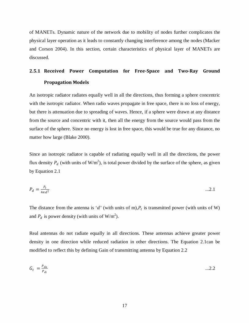
17

of MANETs. Dynamic nature of the network due to mobility of nodes further complicates the

physical layer operation as it leads to constantly changing interference among the nodes (Macker

and Corson 2004). In this section, certain characteristics of physical layer of MANETs are

discussed.

2.5.1 Received Power Computation for Free-Space and Two-Ray Ground

Propagation Models

An isotropic radiator radiates equally well in all the directions, thus forming a sphere concentric

with the isotropic radiator. When radio waves propagate in free space, there is no loss of energy,

but there is attenuation due to spreading of waves. Hence, if a sphere were drawn at any distance

from the source and concentric with it, then all the energy from the source would pass from the

surface of the sphere. Since no energy is lost in free space, this would be true for any distance, no

matter how large (Blake 2000).

Since an isotropic radiator is capable of radiating equally well in all the directions, the power

flux density 𝑃𝑃𝑑𝑑 (with units of W/m2), is total power divided by the surface of the sphere, as given

by Equation 2.1

𝑃𝑃𝑑𝑑 = 𝑃𝑃𝑡𝑡4𝜋𝜋𝑑𝑑2 ...2.1

The distance from the antenna is ‘𝑑𝑑’ (with units of m),𝑃𝑃𝑡𝑡 is transmitted power (with units of W)

and 𝑃𝑃𝑑𝑑 is power density (with units of W/m2).

Real antennas do not radiate equally in all directions. These antennas achieve greater power

density in one direction while reduced radiation in other directions. The Equation 2.1can be

modified to reflect this by defining Gain of transmitting antenna by Equation 2.2

𝐺𝐺𝑡𝑡 = 𝑃𝑃𝑑𝑑𝑑𝑑𝑃𝑃𝑑𝑑𝑑𝑑

...2.2

18

Where, 𝐺𝐺𝑡𝑡 is the gain of transmitting antenna (with units of dBi), 𝑃𝑃𝑑𝑑𝑑𝑑 is the power density of

real antenna (with units of W/m2) and 𝑃𝑃𝑑𝑑𝑑𝑑 is the power density of an isotropic antenna (with units

of W/m2).

Hence, Equation 2.1 can be modified to Equation 2.3 as

𝑃𝑃𝑑𝑑 = 𝑃𝑃𝑡𝑡 𝐺𝐺𝑡𝑡4𝜋𝜋𝑑𝑑2 ...2.3

On the receiving side, the receiving antenna absorbs some of the energy from radio waves that

pass through it. The power extracted from the wave by a receiving antenna depends both on its

physical size and gain (Blake 2000). The effective area (𝐴𝐴𝑒𝑒) of the antenna can be represented by

Equation 2.4 as

𝐴𝐴𝑒𝑒 = 𝑃𝑃𝑟𝑟𝑃𝑃𝑑𝑑

...2.4

Where, 𝐴𝐴𝑒𝑒 is the effective area (with units of m2), and is related to the physical size of the

antenna. 𝑃𝑃𝑟𝑟 is the power delivered to the receiver (with units of W), and 𝑃𝑃𝑑𝑑 is power density

(with units of W/m2).

Combining Equation 2.3 and 2.4 gives Equation 2.5 as

𝑃𝑃𝑟𝑟 = 𝐴𝐴𝑒𝑒𝑃𝑃𝑑𝑑

𝑃𝑃𝑟𝑟 = 𝐴𝐴𝑒𝑒 𝑃𝑃𝑡𝑡 𝐺𝐺𝑡𝑡4𝜋𝜋 𝑑𝑑2 ...2.5

The effective area of receiving antenna can also be represented by Equation 2.6 (Blake 2000)

𝐴𝐴𝑒𝑒 = 𝜆𝜆2𝐺𝐺𝑟𝑟4𝜋𝜋

...2.6

Where,𝜆𝜆 is the wavelength in m (meter) and 𝐺𝐺𝑟𝑟 is the gain of the receiving antenna in dBi.

Combining Equation 2.5 and Equation2.6, the power delivered at the receiver 𝑃𝑃𝑟𝑟 can be

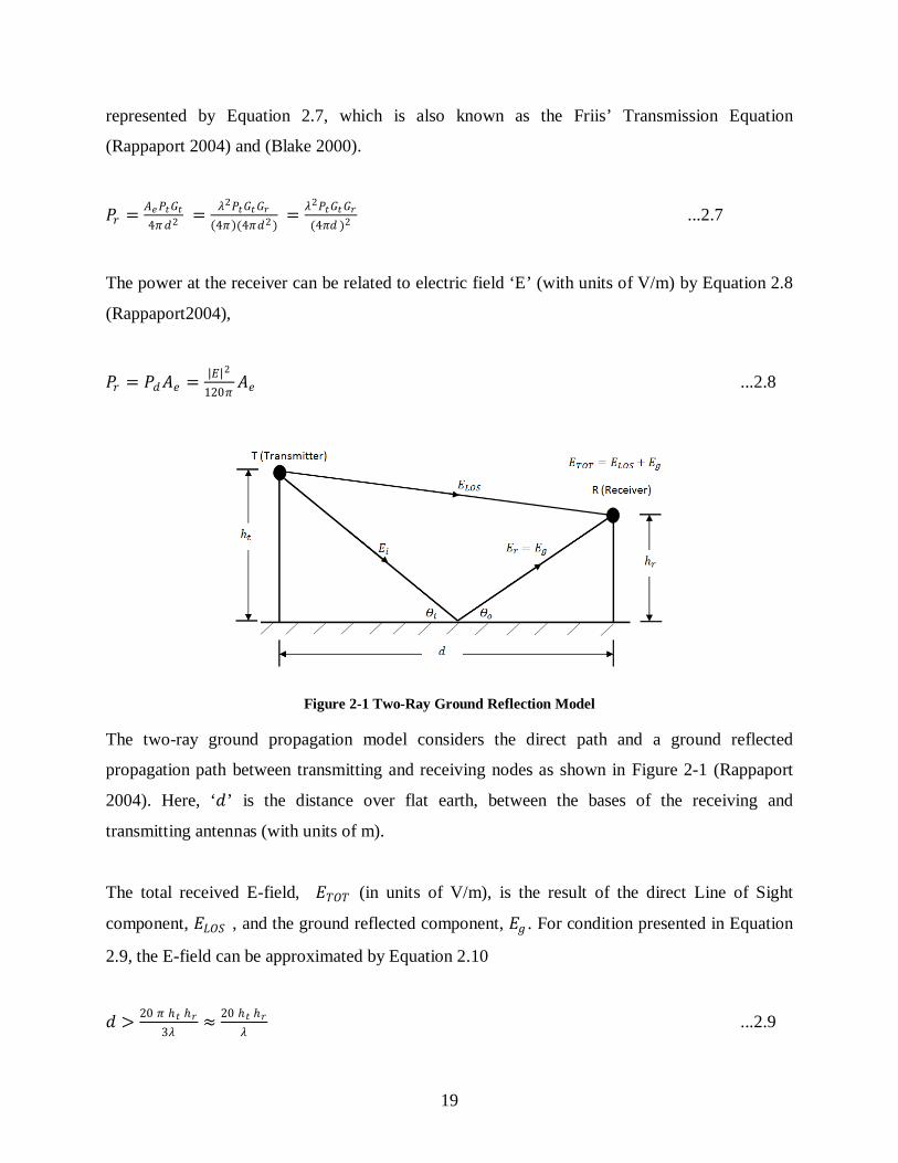
19

represented by Equation 2.7, which is also known as the Friis’ Transmission Equation

(Rappaport 2004) and (Blake 2000).

𝑃𝑃𝑟𝑟 = 𝐴𝐴𝑒𝑒 𝑃𝑃𝑡𝑡 𝐺𝐺𝑡𝑡4𝜋𝜋 𝑑𝑑2 = 𝜆𝜆2𝑃𝑃𝑡𝑡 𝐺𝐺𝑡𝑡 𝐺𝐺𝑟𝑟

(4𝜋𝜋)(4𝜋𝜋𝑑𝑑2 ) = 𝜆𝜆2𝑃𝑃𝑡𝑡 𝐺𝐺𝑡𝑡 𝐺𝐺𝑟𝑟

(4𝜋𝜋𝑑𝑑 )2 ...2.7

The power at the receiver can be related to electric field ‘E’ (with units of V/m) by Equation 2.8

(Rappaport2004),

𝑃𝑃𝑟𝑟 = 𝑃𝑃𝑑𝑑 𝐴𝐴𝑒𝑒 = |𝐸𝐸|2

120𝜋𝜋𝐴𝐴𝑒𝑒 ...2.8

Figure 2-1 Two-Ray Ground Reflection Model

The two-ray ground propagation model considers the direct path and a ground reflected

propagation path between transmitting and receiving nodes as shown in Figure 2-1 (Rappaport

2004). Here, ‘𝑑𝑑’ is the distance over flat earth, between the bases of the receiving and

transmitting antennas (with units of m).

The total received E-field, 𝐸𝐸𝑇𝑇𝑇𝑇𝑇𝑇 (in units of V/m), is the result of the direct Line of Sight

component, 𝐸𝐸𝐿𝐿𝑇𝑇𝐿𝐿 , and the ground reflected component, 𝐸𝐸𝑔𝑔 . For condition presented in Equation

2.9, the E-field can be approximated by Equation 2.10

𝑑𝑑 > 20 𝜋𝜋 ℎ𝑡𝑡 ℎ𝑟𝑟3𝜆𝜆

≈ 20 ℎ𝑡𝑡 ℎ𝑟𝑟𝜆𝜆

...2.9

20

𝐸𝐸𝑇𝑇𝑇𝑇𝑇𝑇 ≈ 2 𝐸𝐸0 𝑑𝑑0𝑑𝑑

2𝜋𝜋ℎ𝑡𝑡 ℎ𝑟𝑟𝜆𝜆𝑑𝑑

≈ 𝑘𝑘𝑑𝑑2 ...2.10

Where, 𝐸𝐸𝑇𝑇𝑇𝑇𝑇𝑇 is measured in V/m,𝑑𝑑0 is the reference distance (with units of m), ‘𝑘𝑘’ is a constant

related to 𝐸𝐸0 (electric field in free space with units of V/m),ℎ𝑡𝑡 is the height of transmitter

antenna (with units of m), ℎ𝑟𝑟 is the height of receiver antenna (with units of m),the wavelength𝜆𝜆

(with units of m) and the distance 𝑑𝑑 (with units of m) between transmitter and receiver.

The received power at a distance ‘𝑑𝑑’ is related to the square of the electric field through Equation

2.8. From the combination of Equations 2.7, 2.8 and 2.10, the received power at a distance ‘𝑑𝑑’

from the transmitter can be expressed as

𝑃𝑃𝑟𝑟 = 𝑃𝑃𝑡𝑡 𝐺𝐺𝑡𝑡𝐺𝐺𝑟𝑟ℎ𝑡𝑡

2ℎ𝑟𝑟2

𝑑𝑑4 ...2.11

Detailed derivation of Equation 2.11 is provided in (Rappaport 2004).

2.5.2 Relevance of Friis’ Transmission Formula for Directional Antenna

The Friis’ Transmission Formula is presented in Equation 2.7, where, 𝐺𝐺𝑡𝑡 and 𝐺𝐺𝑟𝑟 are the gains of

transmitting and receiving antennas respectively. The gain of an antenna is represented as the

product its efficiency and directivity (Shaw 2013), as shown in Equation 2.12.

𝐺𝐺𝑡𝑡 = 𝑒𝑒𝐷𝐷𝑡𝑡and𝐺𝐺𝑟𝑟 = 𝑒𝑒𝐷𝐷𝑟𝑟 ...2.12

Efficiency can be represented as in Equation 2.13

𝑒𝑒 = 𝑅𝑅𝑑𝑑𝑑𝑑𝑑𝑑𝑑𝑑𝑡𝑡𝑒𝑒𝑑𝑑 𝑃𝑃𝑜𝑜𝑃𝑃𝑒𝑒𝑟𝑟𝐼𝐼𝐼𝐼𝐼𝐼𝐼𝐼𝑡𝑡 𝑃𝑃𝑜𝑜𝑃𝑃𝑒𝑒𝑟𝑟

...2.13

The directivity of an antenna is the measure of antenna radiation in a given direction relative to

an isotropic antenna, which radiates uniformly in all the directions. Directivity is defined as the

21

ratio of radiation intensity of the antenna 𝑈𝑈 measured in Watt per steradian (𝑊𝑊 ⋅ 𝑠𝑠𝑟𝑟−1), in a

given direction or in the direction of maximum radiation, to the isotropic radiation intensity

𝑈𝑈𝑜𝑜 (𝑊𝑊 ⋅ 𝑠𝑠𝑟𝑟−1).

For total radiated power 𝑃𝑃, radiation intensity can be represented by Equation 2.14, where, Ω is

the projected solid angle of the antenna measured in steradian (𝑠𝑠𝑟𝑟).

𝑈𝑈 = 𝑃𝑃Ω� (𝑊𝑊 ⋅ 𝑠𝑠𝑟𝑟−1) ...2.14

The radiation intensity of an isotropic antenna can be represented by Equation 2.15, because

isotropic antenna radiates equally well in all the directions.

𝑈𝑈𝑜𝑜 = 𝑃𝑃4𝜋𝜋� (𝑊𝑊 ⋅ 𝑠𝑠𝑟𝑟−1) ...2.15

Therefore, the directivity (𝐷𝐷) of an antenna is represented by Equation 2.16

𝐷𝐷 = 𝑈𝑈𝑈𝑈𝑜𝑜

= �𝑃𝑃Ω

� ⋅ �4𝜋𝜋𝑃𝑃

� = �4𝜋𝜋Ω

� ...2.16

It must be noted from Equation 2.16 that narrower the beam solid angle, higher will be the

directivity of the antenna. Detailed explanation about relevance of Friis transmission formula for

directional antenna is given in (Shaw 2013).

2.5.3 Ranges Related to Wireless Medium

While in wired networks all the nodes are connected with each other through cable to exchange

data, in wireless networks, nodes fall in three following ranges (Xu, Gerla and Bae 2003) and

(Seo et al. 2005):

1. Transmission range: It is also known as communication range. This is the distance

between two nodes within which the nodes can successfully communicate with each

22

other. This range mainly depends on transmission power, receiver sensitivity and channel

attenuation

2. Carrier sensing range: This is the distance over which a node can identify/sense the

presence of a signal in the medium. At this distance, while the signal can be sensed by the

node sensing the medium, it may not be strong enough to be interpreted correctly. This

property is used in IEEE 802.11 MAC to avoid interference and corruption of packets

since a node needs to sense the carrier/medium to be free before signal transmission

3. Interference range: This is the distance within which communication between different

nodes interfere with each other leading to deterioration of the signal. Interference is

generally measured at the receiver

Transmission range and carrier sense range depend on the transmission power and receiver

sensitivity, and can be calculated in advance. However, interference range constantly varies in

MANETs due to mobility of nodes.

The interference range can be calculated based on Equation 2.11, as explained in (Xu, Gerla and

Bae2003). Therefore, the interference range Ri measured in meters (m), can be represented by

Equation 2.17 as,

𝑅𝑅𝑑𝑑 = � 𝑇𝑇𝐿𝐿𝑆𝑆𝑅𝑅𝑘𝑘 × 𝑑𝑑 ...2.17

Where, 𝑑𝑑 is the distance between intended transmitter and receiver node measured in meter

(m), 𝑇𝑇𝐿𝐿𝑆𝑆𝑅𝑅 is the threshold SNR measured in decibel (dB) and 𝑘𝑘 is a constant which represents

how fast the signal decays. This relation is used to measure interference range for

omnidirectional (Xu, Gerla and Bae 2003) and directional (Hong-Ning et al. 2008)

communication.

2.5.4 Types of Antenna

Another important component of the physical layer of nodes in MANET is the antenna which is

used to transmit and receive data over the wireless medium. The antennas used by the nodes in

23

MANETs are mainly of two types (Kumar, Arunan and Balakrishnan 2003) and (Choudhury et

al. 2006)

1. Omnidirectional

2. Directional

Omnidirectional antennas: An isotropic antenna is an ideal antenna which radiates power

equally in all directions. In any plane of dimensional space, the resulting radiation pattern of

isotropic antenna is circular in shape. An omnidirectional antenna is a special case of isotropic

antenna. The radiation pattern of an omnidirectional antenna is circular in shape in only selected

planes of 3D space. A typical omnidirectional radiation pattern of an antenna is shown in Figure

2-2. From the radiation pattern of the omnidirectional antenna, it can be observed that such

antennas radiate uniformly in one plane and the radiated power decreases with elevation angle

above and below the plane. The radiated power drops to zero along the antenna axis, giving it

doughnut shape when viewed from front.

Figure 2-2 Radiation Pattern of an Omnidirectional Antenna (Blake 2000)

This item has been removed due to 3rd Party Copyright. The unabridged version of the thesis can be viewed in the Lanchester Library Coventry University.

24

When a node transmits using omnidirectional antenna, the transmitted signal reaches all the

nodes present within the communication range of the transmitter whether the signal is meant for

all of them or not. This induces interference among the nodes in the network. These antennas are

used for applications where it is required to transmit and receive equally well in all the directions

in a plane. Some of the applications where these antennas are mainly used are radio

broadcasting, wireless computer network communication, base stations, cell phones and cordless

phones (Ramanathan 2004).

Directional antenna: Unlike omnidirectional antennas, directional antennas radiate higher

power in one direction when compared to other directions. These are also called as beamforming

antennas. This capability allows these antennas to increase transmit and receive range in a

particular direction for given power, when compared to omnidirectional antennas (Ramanathan

2004). The radiation pattern of the directional antenna is shown in the Figure 2-3.

As seen from Figure 2-3, radiation pattern of the directional antenna is composed of different

lobes such a main lobe, side lobe and back lobe. Main lobe is the one with highest radiation

intensity, while radiation intensity in side and back lobes is low. Null represents the region with

significantly lesser radiation power. The main lobe is also called as the beam of the antenna and

Θ represents the beam angle in degrees (Ramanathan 2004).

Figure 2-3 Radiation Pattern of a Directional Antenna

Directional antenna increases the transmission and reception range of the antenna and reduces

interference with other nodes as the transmitter can direct its beam in the direction of the

intended receiver (Ramanathan 2004).

25

Figure 2-4 Directional Antenna Beamforming and Null Steering

As seen from Figure 2-4, directional antenna can direct its main lobe (beam) towards intended

receiver node and null towards the interfering node.

Types of Directional Antennas

There are mainly two types of directional antennas namely switched beam and steered beam

(Ramanathan 2004). In case of switched beam antennas, the 360o angular coverage around the

antenna in a plane is divided into equal number of sectors such that each antenna element

transmits or receives in one sector. The antenna sectors are also known as antenna beams. If

there are ‘n’ beams, the beamwidth of each beam would be360 𝑜𝑜

𝐼𝐼.

Figure 2-5 Beams in a Switched Beam Antenna

The Figure 2-5shows a switched beam antenna with 8 beams, each with beam angle of 45o.

Based on the direction of transmission or reception, the antenna chooses an appropriate beam.

26

Figure 2-6 Steered Beam Antenna

In steered beam antennas, there is only one beam that can be steered in any required direction.

As shown in Figure 2-6, these antennas can steer their beams to avoid interaction and

interference from unwanted nodes by steering the main lobe and side lobes away from the

interferer, also known as null steering (Ramanathan 2004).

2.5.5 Antenna Characteristics

Radiation Pattern F (𝜽𝜽, 𝝓𝝓): Radiation pattern is the variation of radiated field of antenna as a

function of Elevation (𝜃𝜃) and Azimuth (𝜙𝜙) angles measured in degrees (Mott 1986) and

(Bellofiore et al. 2002).

Figure 2-7 Beamwidth of an Antenna (Blake 2000)

Beamwidth: It is the angular separation between the -3dB points on either side of the direction

of peak gain of a radiation pattern. Beamwidth of an antenna is measured in degrees. Smaller the


27

beamwidth of an antenna, higher will be its gain (Ramanathan 2004). The 3 dB beamwidth of an

antenna is shown in Figure 2-7.

Figure 2-8 Vertical Polarisation (Chilukuri 2012)

Polarisation: It is defined as the orientation of the electric field of the wave radiated by the

antennas. There are mainly three types of antenna polarisations namely linear, circular and

elliptical. Linearly polarised antennas mainly have vertical and horizontal polarisation. As seen

from Figure 2-8 the orientation of the electric field in vertically polarised antenna is

perpendicular to the ground.

Figure 2-9 Horizontal Polarisation (Chilukuri 2012)

It is shown in Figure 2-9 that the electric field for a horizontally polarised antenna is parallel to

the ground. Vertical and horizontal polarisations are orthogonal to each other. For maximum

possible received power of a communication system, the polarisations of the antennas at two

communicating nodes should be same (Mott 1986) and (Dhande 2009).



28

Gain: The gain of an antenna is the relation between radiation intensity of the antenna in a given

direction to the intensity produced by an isotropic antenna having equal radiation in all the

directions without any losses (Shaw 2013). Gain is measured in dBi.

Directivity D: It is the measure of directionality of the radiation pattern of an antenna. It is the

ratio of power density radiated by an antenna in the direction of strongest radiation to the power

density radiated by an isotropic antenna (Shaw 2013). Directivity is measured in dBi.

2.5.6 Benefits of using Directional Antenna in MANETs

Due to antenna beamforming and increased gain when compared to omnidirectional antennas,

for a given power, directional antennas provide many benefits to MANETs. The benefits of using

directional antennas in MANETs are as follows

1. Reduced interference: As nodes in wireless networks are highly prone to interference,

narrow beamwidth of directional antennas helps in achieving reduced interference among

the nodes in the network. This helps in enhancing performance of the network in terms of

throughput (Saha and Johnson 2004)

2. Spatial reuse: Directional antennas provide better spatial reuse due to antenna

beamforming. This helps in reduced interference among the nodes as well as reduction in

the number of nodes suffering from the problem of exposed nodes, wherein a node

located within communication range of two communicating nodes needs to wait for the

ongoing communication to complete before it can initiate new communication, in order

to avoid corruption of packets. With antenna beamforming the number of nodes

undergoing exposed node problem reduces, thus increasing network efficiency and

capacity by allowing multiple simultaneous communications in the network (Korakis,

Jakllari and Tassiulas 2003). Reduction in exposed node problem with directional

antenna is explained in detail in Section2.6.4

29

3. Increased communication range: Gain of directional antennas is higher than that of

omnidirectional antennas (Choudhury et al. 2002). Due to increased gain and antenna

beamforming, communication range of directional antenna is higher when compared to

omnidirectional antennas for a given input power (Ramanathan 2004)

4. Energy efficiency: As directional antennas provide increased communication range for a

given input power when compared to omnidirectional antennas, for a known

communication range, input power can be reduced when directional antennas are used.

This helps in reducing energy consumption by the node. This feature is very important in

MANETs where the nodes rely on limited battery power while on the move (Ramanathan

2004)

5. Reduced latency: In MANETs, when two nodes need to communicate with each other, it

may be required for the message to pass through intermediate nodes. While the

intermediate nodes help in forwarding of message, they induce per hop delay leading to

increased end-to-end delay. With increased communication range, nodes using

directional antennas can communicate over longer distances thus avoiding certain or all

intermediate nodes to send the message to the receiver node. This helps in achieving

reduced network latency and enhanced network efficiency (Saha and Johnson 2004)

6. Increased security: Directional antennas provide resistance against jamming attacks.

Also, due to increased communication range, nodes using directional antennas acquire

reduced dependence on intermediate nodes for communication. This helps in avoiding the

data being passed through malicious nodes(Hu and Evans 2004), (Lu et al. 2008) and (Lu

et al. 2010)

7. Increased throughput of network: When directional antenna is used during reception of

signals, it reduces interference due to neighbouring transmitters. This leads to higher

value of Signal to Interference and Noise Ratio (SINR) of the packet being received. If

the SINR of the received packets is below certain threshold, then it cannot be correctly

detected at the receiver, leading to reduction in throughput of the network. As the packets

30

received at the nodes using directional antenna have higher SINR, it can be concluded

that use of directional antenna helps in increasing the throughput of the network when

compared to omnidirectional antennas (Nasipuri, Li and Sappidi2002)

It is proved by (Choudhury et al. 2002), that (𝐺𝐺𝑑𝑑 × 𝐺𝐺𝑑𝑑 ≥ 𝐺𝐺𝑑𝑑 × 𝐺𝐺𝑜𝑜 = 𝐺𝐺𝑜𝑜 × 𝐺𝐺𝑑𝑑 ≥ 𝐺𝐺𝑜𝑜 × 𝐺𝐺𝑜𝑜),

where, 𝐺𝐺𝑑𝑑 is the gain of directional antenna (measured in dBi) and 𝐺𝐺𝑜𝑜 is the gain of

omnidirectional antenna (measured in dBi). Hence, it can be inferred that while trying to

establish communication, two nodes operating in omnidirectional mode may fall out of the

communication range of each other as the product of their gains is smaller than the case where at

least one or both nodes operate in directional mode. The product of gains of two communicating

nodes, such that both the nodes communicate using directional antenna is highest when

compared to the cases where one or both nodes use omnidirectional antennas. Communication

between two nodes is termed as directional communication when both the nodes (transmitter and

receiver) communicate using directional antenna such that transmitting beam of the transmitting

and receiving nodes points towards each other (Takata, Bandai and Watanabe 2005).

2.5.7 Power Control with Directional Antenna in MANETs

Another important feature that the physical layer of a node in MANET deals with is transmitter

and receiver power (Shaw 2013). From Friis’ transmission formula relations given in Equation

2.7, the following relations hold true,

𝑃𝑃𝑟𝑟 ∝ 𝑃𝑃𝑡𝑡 , 𝐺𝐺𝑡𝑡 𝑑𝑑𝐼𝐼𝑑𝑑 𝐺𝐺𝑟𝑟 , while 𝑃𝑃𝑟𝑟 ∝ 1𝑑𝑑

If directional antenna is used at both receiver and transmitter, then increased gain (when

compared to omnidirectional antenna) provides increased signal power at the receiver. This in

turn helps in achieving better signal strength and enhanced QoS at the receiver. Also, keeping

receiver and transmitter power constant, increased gain at the transmitter due to use of

directional antenna, enables the transmitter signal to cover longer communication range.

Therefore, in order to achieve an aprior range, the transmitter power can be reduced. This helps

in conservation of battery power which is a limited source of energy in mobile nodes.

31

As the nodes participating in MANET communication depend upon limited battery resources,

transmission power control can be utilised to reduce energy consumption at the nodes

(Ramanathan 2004). By doing this, range of directional antenna can be reduced such that it is just

enough to communicate with the required node. Apart from energy conservation, transmission

power control also helps in reducing interference among transmitting nodes located within the

communication range of each other. Dynamic power control feature can allow a node to either

decrease or increase the transmission power to maintain communication links (Ramanathan

2004). As nodes participating in MANET communication are mobile, transmitter can reduce its

transmission power if the communicating nodes are near/well within the maximum

communication range of each other. This helps in conserving energy at the transmitting node. If

the nodes being mobile, start moving away from each other, then the transmitting node can

increase its transmission power to avoid the disruption of communication link. If transmission

power needs to be increased to maintain communication links among mobile nodes, energy

consumption at the node can increase (Ramanathan 2004).

The most crucial task of implementing power control in MANETs is to estimate the required

transmission power which can guarantee just adequate SINR for the packet at the receiver. As

the nodes in MANETs may keep moving constantly, the required SINR at the receiver also keeps

changing constantly (Ramanathan 2001).

Many researchers have studied power control in MANETs using directional antenna. Two of the

most popular power control schemes have been proposed in (Ramanathan 2001) and (Arora,

Krunz, and Muqattash2004). These schemes are also adopted by many other protocols for power

control in ad-hoc networks. In the paper (Ramanathan 2001) a MAC protocol is proposed which

employs adequate power control while using directional antenna on per-packet basis. It is

demonstrated through simulation results that use of directional antenna with power control helps

in enhancing throughput of network and energy conservation when compared to omnidirectional

antenna. In the proposed MAC protocol of (Ramanathan 2001), the RTS and CTS packets are

transmitted with maximum transmission power, while data and acknowledgement packets are

transmitted using power control. When a node receives the RTS packet, it computes the

difference between minimum required SINR (SINRmin) and SINR with which the RTS is

32

received. This difference is sent to the transmitter through CTS packet. Based on this

information, the transmitter reduces transmission power for the data packet by a value of the

difference minus a margin of δ dB, which does not exceed the maximum transmission power

level of the transmitter. This helps in achieving the SINR measured at the receiver to be δ dB

higher than SINRmin. The value of δ dB is chosen such that it is sufficient to combat the risk of

packet error due to unexpected interference, fading and node mobility, while avoiding wastage of

transmitter power. This method is also adopted in (Nasipuri, Li, and Sappidi 2002), to achieve

power control while using directional antennas.

The Directional Medium Access Protocol (DMAP) proposed in (Arora, Krunz, and Muqattash

2004) also employs power control. In this protocol, the control and data packets are exchanged

over different channels. While RTS is transmitted omnidirectionally, CTS transmission takes

place directionally. The RTS packet is transmitted omnidirectionally with a fixed initial

transmitter power, by the transmitter. The transmitter computes transmit power such that it is just

enough to overcome path loss and interference and yet is sufficient to achieve required SINR at

the receiver.

In the transmission power control algorithm proposed by (El-Osery et al. 2004), each node

appends its transmission power in the data packet. On receiving this data packet, the receiver

node computes Signal to Interference Ratio (SIR) of the received data packet and calculates the

new transmission power. Every node also maintains a table containing node IDs and their

respective transmission powers. The entries in this table are constantly updated as network is

composed of mobile nodes and its topology changes constantly.

It must be noted that the methods to achieve power control where RTS/CTS packets are

transmitted at maximum transmission power while data and acknowledgement packets are

transmitted with reduced transmission power will lead to asymmetry in communication range.

Similarly, omnidirectional transmission of RTS/CTS packets and directional transmission of data

and acknowledgement packets can also lead to corruption of packets due to asymmetry in gain

and thus asymmetry in communication range as discussed in (Nasipuri et al. 2000) and

(Subramanium and Das 2010).

33

The dual polarised directional communication based DPDA-MAC and DPDA-MRP presented in

this thesis, provide a provision for optional dynamic power control. The nodes maintain location

information of neighbour nodes and RSSI of the broadcast packets received from them in the

Neighbour Table (NT) (as shown in Table 4-1) and can use this information for optional

dynamic power control to achieve energy efficient communication. This feature is optional, and

can be used by nodes in a MANET for energy efficient communication. In the simulations

carried out in Chapters 4, 5, 6 and 7, dynamic power control is not implemented. The simulation

results presented in these chapters do not incorporate dynamic power control. However, in

future, the implemented DPDA-MAC and DPDA-MRP protocols can be upgraded to incorporate

dynamic power control by using information available in NT, for energy efficient

communication.

2.5.8 Use of Dual Polarised Directional Antenna in Wireless Networks

As mentioned in Section2.5.5, polarisation of an electromagnetic wave is defined as the

orientation of the electric field vector. An antenna can have different polarisations such as

circular, elliptical, vertical and horizontal. In this thesis vertical and horizontal polarisations, also

known as linear polarisation, of an antenna are used to deal with the problem of interference,

deafness and exposed nodes. An efficient multipath routing protocol is also proposed using dual

polarised directional antenna.

Antennas typically generate electromagnetic waves which are either vertically or horizontally

polarised. Polarisation is a characteristic of both directional and omnidirectional antennas. Direct

path between transmitter and receiver nodes can preserve the original polarisation of the

wave/signal, thus maintaining the polarisation of the signal with which it was transmitted and

while it was received. Therefore, two communicating nodes must be tuned to same polarisation

(either vertical or horizontal) (Khalid et al. 2011). However, the polarisation of a wave/signal

changes while it propagates through the wireless medium, as it undergoes reflection, refraction,

diffraction and scattering. This leads to cross-coupling or depolarisation wherein some of the

energy of the propagating signal gets transferred to the orthogonal polarisation component. Ratio

of the power in desired polarisation to that transferred in the orthogonal polarisation is known as

34

the Cross-Polarisation Ratio (CPR), measured in dB. CPR for a vertically or horizontally

polarised signal can be represented through the Equation 2.18 (Khalid et al. 2011)

𝐶𝐶𝑃𝑃𝑅𝑅 = 𝑃𝑃(𝑐𝑐)

𝑃𝑃(𝑥𝑥 ) …2.18

Where, 𝑃𝑃(𝑐𝑐) represents the power radiated in desired polarisation (co-polar signal) and 𝑃𝑃(𝑥𝑥)

represents the power transferred to the polarisation orthogonal to the desired polarisation (cross-

polar component).

While travelling through the medium, a signal gets deteriorated due to pathloss, scattering,

interference, mismatch between polarisations of transmitter and receiver and depolarisation. In

case of directional antennas, transmitter-receiver beam pointing error also leads to deterioration

of signal. Relation between CPR and distance travelled by the signal can be represented by

Equation 2.19.

𝐶𝐶𝑃𝑃𝑅𝑅 = 𝑑𝑑−𝑑𝑑 𝜒𝜒 …2.19

Where, d is the distance measured in meters, a is a constant with value much smaller than 1, 𝜒𝜒 is

a lognormally distributed random variable having µc mean with units of dB and σc standard

deviation with units of dB (Khalid et al.2011).

In (Khalid et al. 2011), the concept of polarisation diversity is used to enhance the performance

of MANETs. In the Cooperative Polarisation Directional Medium Access Control (CPDMAC)

protocol proposed in (Khalid et al. 2011), nodes use directional communication and adapt the

polarisation which offers least interference while communicating with other nodes. Therefore, if

two nodes are communicating over vertical polarisation, other two nodes present within the

range of communicating nodes can choose to communicate over horizontal polarisation to avoid

interference while communicating simultaneously. While the nodes can dynamically choose

appropriate polarisation for communication, they can use only one polarisation (either vertical or

horizontal) at a time. The vertical and horizontal polarisations are considered as two separate

orthogonal channels which can be used for simultaneous communication without causing

35

interference. It is mentioned in (Khalid et al. 2011) that channel orthogonality is maintained for a

distance of 50m-200m in Line Of Sight (LOS) settings for ad-hoc networks while for Non-LOS

(NLOS) settings, orthogonality is reduced due to multipath effects, leading to a CPR of around

8-15dB. For switching between available polarisations, the nodes are required to be equipped

with two linearly polarised antennas with a PIN-diode circuit which is used to switch between

required polarisations. The time taken by the PIN-diode circuit to switch between the two

polarisations is in the order of a few nanoseconds, which is negligible (Khalid et al. 2011).

In this thesis, Dual Polarised Directional Antenna (DPDA) is used for communication between

nodes in a MANET. The proposed concept of dual polarisation is different from polarisation

diversity in CPDMAC. In CPDMAC a node uses one polarisation (either vertical or horizontal

polarisation) at a particular time, while in the proposed dual polarisation method, a node is

capable of using both the polarisations (vertical and horizontal) simultaneously. Therefore, while

a node is communicating with one node using vertical polarisation, it can simultaneously

communicate with another node using horizontal polarisation. This method is explained in detail

in Chapters 5 and 6.

Directional Medium Access Control using Polarisation Diversity Extension (DMAC-PDX) is

proposed in (Yildirim and Liu 2007) for wireless communication in 60GHz band. The authors

use the polarisation characteristic of an antenna to detect the presence of direct path between

transmitter and receiver nodes. In case of the presence of direct path between transmitting and

receiving nodes, the signal polarisation remains same, while signal polarisation changes in case

of reflected paths.

The effect of antenna directivity and polarisation diversity on enhancing the communication

range and throughput of vehicular networks is studied in (Zaggoulos, Nix andHalls2010). For

this study, the authors used vehicles installed with 2x2 MIMO system with a pair of dual-

polarised directional antennas. The studies included different combinations of antenna directivity

and polarisations on the transmitter and receiver nodes. For example, when directional antenna is

used at transmitter and receiver nodes, the polarisation is varied as +/- 45 degree, both vertical

and vertical-horizontal. Similar experiments are carried out with omnidirectional antenna as well.

36

From the experiments, it is concluded that orthogonally polarised directional devices outperform

all other configurations to achieve highest throughput of network.

The concept of polarisation diversity is also used in IEEE 802.11n based MIMO systems to

overcome the ‘Keyhole Effect’, (Vella and Zammit 2010). The effect of polarisation diversity on

the throughput of IEEE 802.11n based MIMO systems is studied. In this study, the authors have

established networks using WLAN standard based hardware in indoor environment. From the

experimental results it is observed that throughput of the network almost doubles when

polarisation diversity is used. Similar study for IEEE 802.11n based MIMO systems is carried

out for long distance outdoor environments in (Paul et al. 2011), where high gain directional

antenna and polarisation diversity are used to study variation in network performance. The study

reveals that by using directional antenna with polarisation diversity, maximum network

throughput is obtained up to a communication distance of 800m in outdoor environments.

Another study on MIMO system utilises bidirectional dual polarised antenna to study the

polarisation behaviour in corridor environment (Keowsawat et al. 2009).

From the above cited research studies, it is observed that the antenna polarisation has been

successfully exploited in wireless networks to achieve high throughput of network. In

polarisation diversity, a node adaptively chooses an appropriate polarisation to have

communication with other node in order to avoid interference with ongoing transmissions of the

neighbouring nodes. However, at any given time, a node can only use one chosen polarisation to

communicate with another node.

In this thesis, the concept of dual polarisation is proposed wherein, a node cannot only choose an

appropriate polarisation to avoid interference with ongoing communication, but also can use

different polarisations to communicate with different nodes simultaneously. Therefore, for

example, while Node A can communicate with Node B using vertical polarisation, Node A can

simultaneously communicate with Node C using horizontal polarisation. This helps in achieving

enhanced network performance and efficiency. This concept of DPDA is used to propose DPDA-

MAC protocol to deal with the problem of exposed node and deafness in MANETs. As efficient

routing is crucial in MANETs, DPDA based Multipath Routing Protocol called DPDA-MRP is

37

also proposed in this thesis. Apart from these two protocols, this thesis proposes a method to

avoid corruption of broadcast packets due to hidden node problem. These broadcast packets are

used to populate neighbour tables which are further used for multipath routing.

2.5.9 Channel Model

On transmission over wireless networks, signals have to deal with different characteristics of the

wireless medium such as interference due to other nodes, pathloss, fading, shadowing, reflection,

refraction, diffraction and scattering. These different phenomena have different characteristics

and affect the signals differently. As all these effects are present in the wireless medium, the end

effect of these different phenomena is modeled as an error probability model for a particular

amount of information, such as number of packets or bits (Boukerche and Bononi 2004) and

(Halford and Chugg 2011).

One such method used to model the probability of error in the physical medium is known as the

Gilbert-Elliot Error Model. This model is used to study the effects of errors introduced during

packet transmission over the wireless medium. The simplest Gilbert-Elliot Error Model is a

Markov chain based channel model which was introduced by Edgar Gilbert and E.O. Elliot to

explain the burst error patterns present is wireless transmission channel. This is a Markov chain

based two state model, as shown in Figure 2-10. The channel model has two states, good and

bad. While good state determines the probability of transmitting the information correctly over

the transmission channel, the bad state denotes the probability of transmitting the information

with error.

Figure 2-10 Two State Markov Channel Model

The Gilbert-Elliot model has been extensively used for simulation of IEEE 802.11 networks. The

technical report titled ‘A Gilbert-Elliot Bit Error Model and The Efficient Use in Packet Level

38

Simulation’, by Technical University Berlin, Telecommunication Network Group, 1999, uses the

Gilbert-Elliot model for simulation of IEEE 802.11 networks.

2.6 MAC Layer in MANETs

The MAC layer in MANETs is concerned with accessing the wireless medium which is shared

among multiple nodes. Characteristics of wireless medium are different from that of wired

medium. While in wired medium, all the nodes are connected to each other through cable, in

wireless networks nodes may not be in each other’s communication range. Nodes in MANETs

are prone to hidden node and exposed node problems (Forouzan 2007).

Traditionally, nodes in MANETs communicate using omnidirectional antenna. Many researchers

have proved the role of directional antennas in enhancing the performance and efficiency of

MANETs. However, use of directional antennas introduces the problems of directional exposed

nodes and deafness. In this section, the problems of hidden nodes, exposed nodes, directional

exposed nodes and deafness are explained. Survey of solutions to overcome these problems is

presented and drawbacks of existing solutions are also discussed.

2.6.1 Introduction to the Hidden Node Problem

In a wireless network, two nodes not within carrier sensing range of each other and unaware of

each other’s presence (hidden from each other) trying to simultaneously communicate with a

third node, may pave way for corruption of packets.

Figure 2-11 Hidden Node Problem

As shown in Figure 2-11, Nodes A and C try to simultaneously communicate with Node B.

Nodes A and C are within the range of Node B and not within the range of each other. Therefore,

39

Nodes A and C are ‘hidden’ from each other. If Nodes A and C simultaneously transmit a data

packet to Node B, then the packets may get corrupted at B, thus leading to an unsuccessful

communication attempt. The nodes may retransmit the broadcast packets. Even then, there are

chances that corruption of packets may take place again. This leads to waste of network

bandwidth and battery energy of nodes. It is essential to solve the hidden node problem, as for

omnidirectional communication; there can be an average of 𝟏𝟏. 𝟑𝟑𝟑𝟑𝑹𝑹𝟐𝟐hidden nodes for any node,

where, R is the transmission range of the node in meters and σ represents the number of nodes

uniformly distributed per unit area (Jayasuriya et. al. 2004).

Many solutions have been proposed to avoid such corruption of packets due to hidden node

problem. A survey of these solutions is presented in Section 2.6.2.

2.6.2 Survey of Methods for Handling Hidden Node Problem

Some of the methods to handle the hidden node problem proposed in literature require two

separate channels for control and data packets. Protocols based on Busy Tone Multiple Access

(BTMA), such as Dual BTMA (DBTMA) by (Haas and Deng 2002) and Receiver Initiated-

BTMA (RI-BTMA) by (Wu and Li 1987) require a message channel and a busy-tone channel.

These solutions require dividing limited available bandwidth into separate control and data

channels, where control channel may not be used as much as the data channel. It is also required

to ensure that the control and data channels do not interfere with each other. Such protocols lead

to increased hardware cost and implementation complexity.

There are Multiple Access Collision Avoidance (MACA) based protocols such as MACA-By

Invitation (MACA-BI) by (Talucci, Gerla and Fratta 1997), MACA for Wireless-LANs

(MACAW) by (Bhargavan et al. 1994) and Floor Acquisition Multiple Access (FAMA) by

(Garcia and Fullmer 1999). Apart from these, there is IEEE 802.11 Distributed Coordination

Function (DCF) based Carrier Sense Multiple Access/Collision Avoidance (CSMA/CA) protocol

explained in Section2.6.3, which is the most common protocol used in wireless networks. None

of these protocols have studied the possibility of corruption of the very first packet transmitted,

without reservation of the medium. While authors in (Talucci, Gerla and Fratta 1997) have

40

briefly discussed about the possibility of corruption of RTS frames due to hidden terminal

problem, their main work deals with corruption of data packets.

While many researchers have worked on broadcasting techniques, most of the work discusses

schemes for rebroadcasting. In one of the paper authored by (Williams and Camp 2002), it is

observed that for avoidance of corruption of broadcast packets due to hidden terminal problem,

exchange of RTS/CTS/Data/ACK is bandwidth expensive and difficult to coordinate. The

authors have also pointed out that the process of clear channel assessment alone is incapable of

preventing corruption of packets due to hidden terminal problem, and an appropriate method is

required to be devised to handle corruption of broadcast packets due to hidden node problem.

The authors present ‘Jitter and RAD’ scheme, where Random Assessment Delays (RAD) at

different nodes attempting to access the communication channel, corruption of broadcast packets

due to hidden node problem. Most of the other literature surveyed in (Williams and Camp 2002)

proposes to limit the number of rebroadcasts. Some of the methods to handle broadcast related

problems are Simplified Multicast Forwarding (SMF) (Macker and Team 2008), Dominant

Pruning (Lim and Kim 2000), Multi-point Relay (Qayyum, Viennot and Laouiti 2000), Scalable

Broadcasting (Peng and Liu 2000) and Ad-hoc Broadcast Protocol (Peng and Liu 2001). All

these protocols require that every node has information about its two hop neighbours. These

protocols require extra transmission overhead, particularly in dense networks, as pointed out in

(Sardouk et al. 2007). Some papers such as (Alagar, Venkatesan and Cleaveland 1995),(Pagani

and Rossi 1997) and (Pagani and Rossi 1999) also suggest the exchange of acknowledgements

for reliable broadcasting, but it can lead to further increase in network traffic, contention and

corruption of packets.

2.6.3 IEEE 802.11 DCF Mechanism

The IEEE 802.11 standard offers the Carrier Sense Multiple Access / Collision Avoidance

(CSMA/CA) mechanism. The IEEE 802.11 standard specifies the physical and MAC layer

functionality for Wireless Local Area Networks (WLANs). In the MAC layer specification, two

types of medium access techniques are mentioned. These are as follows (IEEE LAN/MAN

Standards Committee 1999):

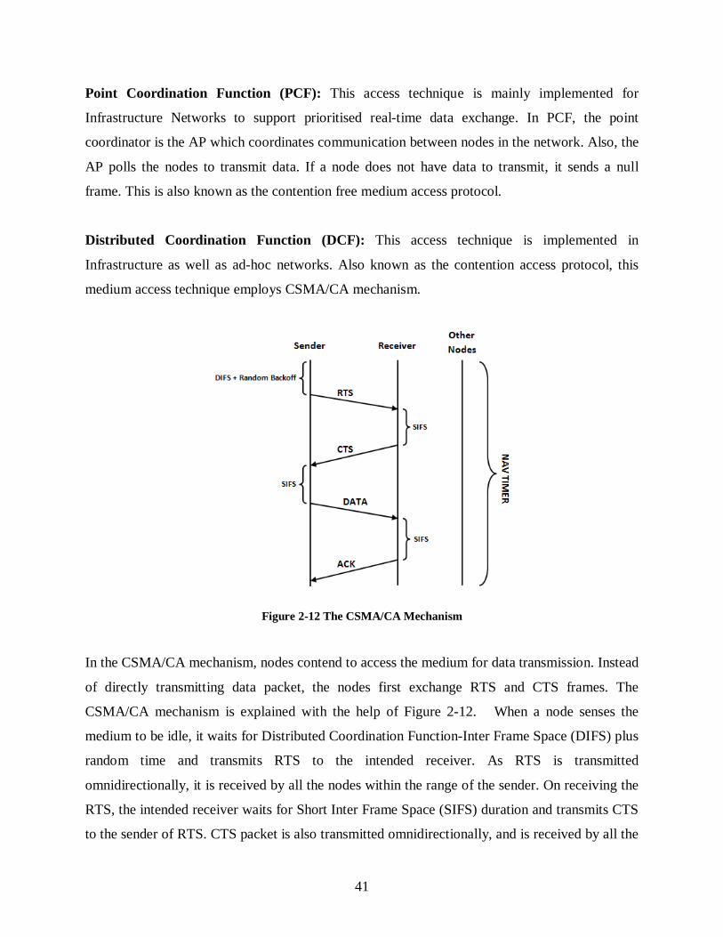
41

Point Coordination Function (PCF): This access technique is mainly implemented for

Infrastructure Networks to support prioritised real-time data exchange. In PCF, the point

coordinator is the AP which coordinates communication between nodes in the network. Also, the

AP polls the nodes to transmit data. If a node does not have data to transmit, it sends a null

frame. This is also known as the contention free medium access protocol.

Distributed Coordination Function (DCF): This access technique is implemented in

Infrastructure as well as ad-hoc networks. Also known as the contention access protocol, this

medium access technique employs CSMA/CA mechanism.

Figure 2-12 The CSMA/CA Mechanism

In the CSMA/CA mechanism, nodes contend to access the medium for data transmission. Instead

of directly transmitting data packet, the nodes first exchange RTS and CTS frames. The

CSMA/CA mechanism is explained with the help of Figure 2-12. When a node senses the

medium to be idle, it waits for Distributed Coordination Function-Inter Frame Space (DIFS) plus

random time and transmits RTS to the intended receiver. As RTS is transmitted

omnidirectionally, it is received by all the nodes within the range of the sender. On receiving the

RTS, the intended receiver waits for Short Inter Frame Space (SIFS) duration and transmits CTS

to the sender of RTS. CTS packet is also transmitted omnidirectionally, and is received by all the

42

nodes in the vicinity of the intended receiver. Based on values of Network Allocation Vector

(NAV) duration present in RTS and CTS frames, other nodes in the vicinity of sender and

receiver start their NAV timers. During this period no other node can initiate communication,

and therefore, corruption of packets due to hidden node problem is avoided.

On receiving the CTS frame, the intended transmitter waits for SIFS duration and transmits data

packet. When the data packet is received successfully, the receiver node waits for SIFS duration

and transmits acknowledgement (ACK). Other nodes in the vicinity of communicating nodes

wait for the ongoing communication to complete based on NAV timer and sense the medium to

be idle. When the medium is sensed idle, the nodes again contend to access it by waiting for

DIFS+ Random Backoff and transmit RTS frame. The sequence of RTS, CTS, Data and ACK

exchange repeats. The DIFS period is 50 µs and SIFS period is 10 µs. Before sending RTS, a

node waits for 50 µs + random time. The random time is measured through Contention Window

(CW) having 31-2013 slots, each 20 µs long (IEEE LAN/MAN Standards Committee 1999) and

(Forouzan 2007).

It must be noted that the CSMA/CA mechanism does not solve the hidden node problem

completely, as the RTS frames simultaneously transmitted from two nodes may get corrupted

due to hidden node problem (Talucci, Gerla and Fratta 1997).

2.6.4 Introduction to the Exposed Node Problem

The CSMA/CA mechanism leads to the exposed node problem (Jayasuriya et al. 2004).This

problem is explained through the scenario presented in Figure 2-13. When two nodes

communicate, other nodes in their vicinity are not allowed to initiate communication till the

NAV timer for ongoing communication expires. As shown in Figure 2-13, Nodes A and B make

use of omnidirectional antenna for communication. Node C is located within the communication

range of Node A, while Node D is located within the communication range of Node B.

While the communication between Nodes A and B takes place, Nodes C and D need to wait for

NAV duration of ongoing communication before they can initiate communication. In this

scenario, Nodes C and D are said to be exposed nodes.

43

Figure 2-13 Exposed Node Scenario

The exposed node problem degrades throughput and efficiency of the network due to delays

among nodes in accessing the medium (Jayasuriya et al. 2004).

Many researchers have proposed the use of directional antenna to overcome interference and

exposed node problem. In (Srisathapornphat and Shen 2003), the authors have studied the

probability of successful RTS-CTS exchange with directional and omnidirectional antennas.

They have proved that the probability of successful transmissions is highest when both RTS and

CTS transmissions are carried out using directional antenna.

2.6.5 Directional Antenna to Reduce the Exposed Node Problem

Occurrence of exposed node problem due to the use of omnidirectional antenna is presented in

Figure 2-13of Section2.6.4. The instances of exposed node problem can be reduced with the use

of directional antenna (Huang et al. 2002). As explained through Figure 2-14, Nodes A and B

make use of directional antenna for communication. Nodes C and D do not fall within the range

of Nodes A and B, and do not get affected by ongoing communication between Nodes A and B.

Figure 2-14 Exposed Node Avoidance using Directional Antenna

44

This enables Nodes C and D to communicate without waiting for Nodes A and B to terminate

ongoing communication. This helps in enhancing the efficiency and performance of the network.

2.6.6 Introduction to the Problem of Directional Exposed Node

It must be noted that while instances of exposed node problem can be reduced by using

directional antennas, it cannot be completely eliminated. If any node falls within the directional

communication range of two nodes, it needs to wait for ongoing communication to end before it

can initiate communication with some other node.

Figure 2-15 Exposed Node in Presence of Directional Communication

In the scenario presented in Figure 2-15, while Nodes A and B communicate using directional

antenna, Node C becomes exposed node and cannot initiate communication with Node D. This is

known as the problem of directional exposed nodes. The problem of directional exposed nodes

is presented in detail in (Takata, Bandai and Watanabe 2005). The authors define a directional

exposed node as a node which is within directional range of a transmitting node and its

omnidirectional sensing range overlaps with directional transmission range of the transmitting

node.

2.6.7 Survey of Methods to Overcome Exposed Node Problem

The exposed node problem has been identified by many researchers while aiming towards

enhancing the Quality of Service (QoS) in wireless networks. The presence of hidden and

exposed node problems degrades network performance of IEEE 802.11 multihop communication

networks (Xu and Saadawi 2001) and (Egbogah, Shi and Fapojuwo 2011). It is observed by (Xu

and Saadawi 2001) that if the number of nodes getting affected by exposed node problem is not

minimised using an appropriate method, the network bandwidth remains underutilised. The

45

authors have also pointed out that in multihop communication, presence of exposed nodes

degrades the performance of the network drastically. Authors suggest reducing the sensing range

of nodes to minimise the occurrence of exposed node problem. However, this method may lead

to more instances of packet corruption in the network due to asymmetry is sensing and

transmission range.

Dual Busy Tone Multiple Access (DBTMA) scheme proposed by (Haas and Deng 2002) and

Receiver-Initiated Busy-Tone Multiple Access (RI-BTMA) scheme proposed by (Wu and Li

1987) are used to overcome the exposed node problem by using busy tones. A method that

allows the nodes participating in an IEEE 802.11 DCF based network to first identify that they

are experiencing exposed node problem and then schedule their transmissions opportunistically

along with other simultaneous transmissions is proposed by (Shukla, Chandran-Wadia and Iyer

2003). The ongoing communication is called primary. An exposed node tries to adjust its

transmission such that they do not interfere with primary transmissions to achieve increased

channel utility. This method is difficult to implement as adjusting the transmissions to avoid

interference on wireless network of mobile nodes is difficult due to dynamic nature of the

network. To eliminate the overhead and exposed node problem caused by RTS/CTS exchange

(Chan and Liew 2006) have proposed physical carrier sensing approach based on MAC

addresses of nodes. A protocol to overcome exposed problem is suggested by (Yeh et al. 2003),

which uses Request To Send (RTS), Object To Send (OTS) and Clear To Send (CTS) frames and

separate control and data channels to overcome exposed node problem. Use of dual channel and

token passing is proposed by (Lu, Fan and Hao 2006) to mitigate the exposed node problem. All

the nodes use separate data and control channels for data and control packet exchange

respectively. Apart from that, nodes use Busy Tone (BT) to avoid other nodes from informing

about absence of token and Token Tone (TT) to allow the nodes having the token join network

communication. With this method, when one pair of nodes exchanges data packets over data

channel, another pair of nodes within the range of first pair can use control channel to exchange

RTS/CTS frames; provided they hold the token. The methods which involve use of separate

control and data channels or tones to mitigate exposed node problem lead to complex transceiver

design. It is also required to ensure that separate channels for control, data or tone information do

not interfere with each other.

46

Power control to mitigate the exposed node problem is proposed by (Zhou and Nettles 2005) and

(Jiang and Liew 2008). The authors have observed that the cause of exposed node problem is

higher carrier sensing range. Therefore, they have proposed power control to shrink the carrier

sensing range, so that the number of nodes affected due to exposed node problem is reduced.

However, as stated earlier, such schemes may lead to more instances of packet corruption due to

asymmetry in carrier sensing and transmission range. Physical layer coding based methods are

also proposed to overcome the problems of hidden and exposed nodes. An attachment coding

and attachment sense based method to combat the problems of hidden and exposed nodes is

presented in (Wang, Wu and Hamdi 2012). The Full-duplex Attachment System (FAST)

proposed in (Wang, Wu and Hamdi 2012) is composed of attachment coding implemented in

physical layer to exchange control information, which is used by attachment sense at MAC layer

to identify the nodes experiencing hidden and exposed node problem. Based on the information

available through attachment sense nodes make decision to access the channel.

Another method to overcome the exposed node problem is the use of directional antenna, which

is supported by many researchers. As observed from Figure 2-13, when omnidirectional antenna

is used, Nodes C and D have to defer communication because of ongoing communication

between Nodes A and B. However, when directional antennas are used, as shown in Figure 2-14,

Nodes C and D can communicate even when the communication between Nodes A and B is in

progress. From the results obtained through simulations carried out in these (Nasipuri, Li and

Sappidi 2002), (Choudhury et al. 2002) and (Takai et al. 2002), it is observed that the use of

directional antenna reduces the instances of exposed node, makes it less severe and increases

spatial reuse. Some of the research work proposing the use of directional antenna to mitigate

exposed node problem is presented here. It is recommended by (Sánchez, Giles and Zander

2001) to use directional transmission for RTS and CTS exchange to reduce the number of

exposed nodes. As an extension to DBTMA, authors in (Huang et al. 2002) proposed

DBTMA/DA which adapts DBTMA to directional communication. The authors prove that the

use of directional antenna along with dual tones, further reduces the occurrence of exposed node

problem and increase the channel capacity. A switched beam directional antenna is used to

exchange RTS, CTS, data, acknowledgement and busy tones, directionally. Use of directional

47

antennas to alleviate the exposed node problem is also supported by (Li et al. 2005). The authors

propose directional exchange of RTS and CTS packets to reduce exposed node problem and

increase capacity of the network. The proposed scheme is tested on wireless mesh networks. To

further prove that the use of directional antenna reduces exposed node problem, (Yamamoto and

Yamamoto 2007) have implemented the Directional Virtual Carrier Sensing (DVCS) proposed

by (Takai et al. 2002), and studied its performance through simulations. Through simulations, the

authors have proved that the use of directional antenna drastically improves throughput of

network by decreasing the instances of exposed nodes and interference.

While it has been proved by available methods in the literature that the use of directional

antennas reduces instances of exposed node problem, it must be noted that the directional

antennas do not mitigate exposed node problem completely. The nodes that fall within the

directional beam of two nodes communicating using directional antenna still experience exposed

node problem. In the experiments carried out for multihop communication using directional

antennas in (Huang et al. 2002), the authors observed that in multihop communication, exposed

node problem suppresses concurrent transmission, even in the presence of directional antenna.

This suppression overhauls the benefits obtained by spatial reuse achieved by using directional

antenna. The occurrence of exposed nodes within the directional beam of communicating nodes

is termed as the Directional Exposed Node Problem in (Takata, Bandai and Watanabe 2005). The

exposed node problem in the presence of directional antennas is clearly explained in (Wang,

Fang and Wu 2005). The authors have proposed Synchronised Directional MAC (SYN-DMAC)

protocol to overcome problems occurring due to use of directional antenna such as directional

hidden and exposed nodes, deafness and head-of-line blocking. However, achieving

synchronised communication in wireless network with mobile nodes is a challenging task.

Another method to overcome the directional exposed node problem is presented in (Hou et al.

2005). In this the authors have proposed to control beam-width, beam-orientation and power

level of the directional antenna. The Authors in (Capone, Martignon and Fratta 2008) have

observed the presence of exposed node problem in the presence of directional antennas. While

the authors have not proposed any solution to overcome the directional exposed node problem in

particular, the Power Controlled Directional Medium Access Control (PCD-MAC) protocol

48

proposed in (Capone, Martignon and Fratta 2008) may overcome this problem through power

control.

2.6.8 Deafness due to Directional Antenna

While the use of directional antenna helps in reducing instances of exposed node and

interference, it leads to another problem known as deafness. The problem of deafness occurs due

to the use of directional antenna. Deafness is caused when a transmitting node repeatedly tries to

send RTS to a destination node, but the destination node does not respond with CTS because it

has formed a directional beam away from the transmitting node (Gossain et al. 2004).

In the scenario shown in Figure 2-16, Node A is communicating with Node B using directional

antenna. Node C being unaware of ongoing communication between Nodes A and B tries to

establish communication link with Node A and sends RTS to it. Since Node A is pointing its

beam towards Node B, Node A does not respond to RTS. Node C waits for CTS, increases

backoff time and retransmits RTS to Node A. However, Node A is deaf towards RTS sent by

Node C. In this process, Node C wastes battery power and network capacity by retransmitting

RTS. The problem of deafness is explained in detail in (Takata, Bandai and Watanabe 2005).

According to the explanation given in (Takata, Bandai and Watanabe 2005), a transmitting node

faces the problem of deafness if the directional beams of the transmitter and its intended receiver

do not overlap, because the intended receiver has formed its beam away from the transmitting

node.

Figure 2-16 Scenario for Deafness

From the above discussion, it is evident that while directional antennas enhance network

performance and efficiency by reducing interference and exposed nodes, the problems of

interference and exposed nodes still exist in the network. Further, use of directional antenna

introduces the problem of deafness in the network.

49

2.6.9 Survey of Solutions to Overcome Deafness

While the use of directional antenna brings in many advantages to MANETs, one of the principal

limitations of using directional antenna is the problem of deafness. As deafness leads to waste of

network resources and adversely affects the network performance, many protocols have been

proposed in literature to deal with the problem of deafness.

To avoid deafness, some authors propose that either RTS, or CTS or both can be transmitted

omnidirectionally to make nodes in the vicinity aware about ongoing communication, while data

and acknowledgement packets can be transmitted directionally to exploit the advantages of

directional antenna. Directional Medium Access Protocol (DMAP) with power control proposed

in (Arora, Krunz and Muqattash 2004) uses omnidirectional RTS and directional CTS

transmission, Beamformed Medium Access Control (BMAC) proposed in (Fakih, Diouris and

Andrieux 2006) uses directional RTS and omnidirectional CTS exchange, while Directional

Medium Access Control using NAV Table (DMAC-NT) protocol proposed in (Jung, Lee and

Han 2009) uses omnidirectional exchange of RTS-CTS and directional exchange for data and

acknowledgement. To detect ongoing communications, nodes use omnidirectional carrier

sensing. While these solutions mitigate deafness, they lead to hidden node problem due to

asymmetry in gains of directional and omnidirectional antennas. The problems arising due to

asymmetry in gain are discussed in (Choudhury et al. 2002), (Subramanium and Das 2010) and

(Abdullah, Cai, and Gebali 2012).To avoid these problems arising due to asymmetry in gain,

authors in (Nasipuri et al. 2000), (Huang et al. 2002), (Choudhury and Vaidya 2004), (Lee et al.

2006) and (Subramanium and Das 2010) have suggested to keep the communication range of

directional and omnidirectional antenna same. To achieve this, the authors have suggested to

reduce the transmission power for the directional transmission. As specified by the authors, this

method not only overcomes the problems arising due to asymmetry in gain of directional and

omnidirectional antennas but also conserves energy at the directional transmitter. These papers

have assumed the gains of directional and omnidirectional antennas as same, to overcome the

problems arising due to asymmetry in gain of directional and omnidirectional antennas.

To deal with deafness the Directional Medium Access Control (DMAC) protocol is proposed

(Ko, Shankarkumar and Vaidya 2000). It is assumed that all the nodes know each other’s

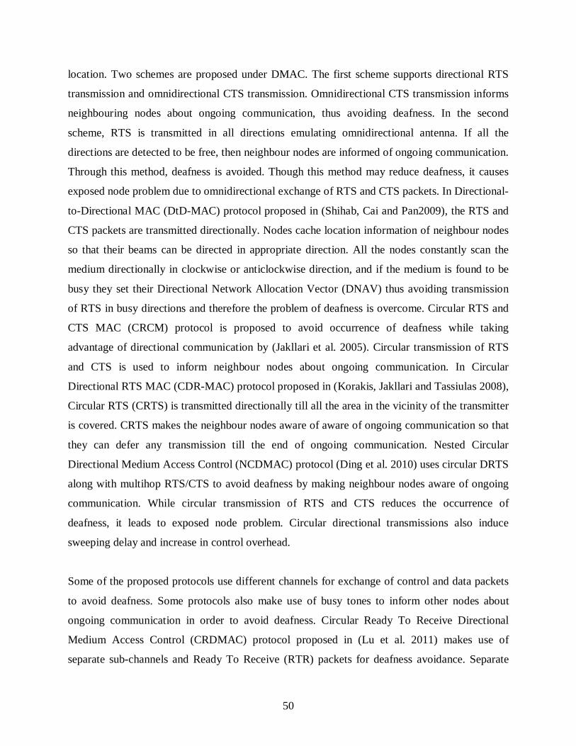
50

location. Two schemes are proposed under DMAC. The first scheme supports directional RTS

transmission and omnidirectional CTS transmission. Omnidirectional CTS transmission informs

neighbouring nodes about ongoing communication, thus avoiding deafness. In the second

scheme, RTS is transmitted in all directions emulating omnidirectional antenna. If all the

directions are detected to be free, then neighbour nodes are informed of ongoing communication.

Through this method, deafness is avoided. Though this method may reduce deafness, it causes

exposed node problem due to omnidirectional exchange of RTS and CTS packets. In Directional-

to-Directional MAC (DtD-MAC) protocol proposed in (Shihab, Cai and Pan2009), the RTS and

CTS packets are transmitted directionally. Nodes cache location information of neighbour nodes

so that their beams can be directed in appropriate direction. All the nodes constantly scan the

medium directionally in clockwise or anticlockwise direction, and if the medium is found to be

busy they set their Directional Network Allocation Vector (DNAV) thus avoiding transmission

of RTS in busy directions and therefore the problem of deafness is overcome. Circular RTS and

CTS MAC (CRCM) protocol is proposed to avoid occurrence of deafness while taking

advantage of directional communication by (Jakllari et al. 2005). Circular transmission of RTS

and CTS is used to inform neighbour nodes about ongoing communication. In Circular

Directional RTS MAC (CDR-MAC) protocol proposed in (Korakis, Jakllari and Tassiulas 2008),

Circular RTS (CRTS) is transmitted directionally till all the area in the vicinity of the transmitter

is covered. CRTS makes the neighbour nodes aware of aware of ongoing communication so that

they can defer any transmission till the end of ongoing communication. Nested Circular

Directional Medium Access Control (NCDMAC) protocol (Ding et al. 2010) uses circular DRTS

along with multihop RTS/CTS to avoid deafness by making neighbour nodes aware of ongoing

communication. While circular transmission of RTS and CTS reduces the occurrence of

deafness, it leads to exposed node problem. Circular directional transmissions also induce

sweeping delay and increase in control overhead.

Some of the proposed protocols use different channels for exchange of control and data packets

to avoid deafness. Some protocols also make use of busy tones to inform other nodes about

ongoing communication in order to avoid deafness. Circular Ready To Receive Directional

Medium Access Control (CRDMAC) protocol proposed in (Lu et al. 2011) makes use of

separate sub-channels and Ready To Receive (RTR) packets for deafness avoidance. Separate

51

sub-channels are used for exchange of data and control packets. Circular directional transmission

of RTR takes place over the control sub-channel to inform neighbour nodes about end of

ongoing communication so that nodes can start RTS transmission to the mentioned Node ID.

Dual-Sensing Directional Medium Access Control (DSDMAC) protocol (Abdullah, Cai and

Gebali 2012), uses two types of busy-tone signals, BT1 and BT2 to solve hidden node and

deafness problems. These busy tones are transmitted by the pair of communicating nodes in the

direction of all possible transmitter and receiver nodes. Some more protocols which use busy

tones to avoid deafness are Busy Tone-Directional Medium Access Control (BT-DMAC) by

(Dai, Ng and Wu 2007), Tone Dual Channel Directional Medium Access Control

(ToneDUDMAC) by (Lee et al. 2006), ToneDMAC proposed by (Choudhury and Vaidya 2004)

and Dual Busy Tone Multiple Access using Directional Antenna (DBTMA/DA) proposed by

(Huang et al. 2002). Main disadvantage of tone based protocols is that these protocols require

separate channels for transmission of tones and data. This leads to increased cost and complex

implementation.

Some other methods which do not rely on tones or circular transmission of RTS/CTS are also

proposed in literature. Opportunistic Directional MAC (OPDMAC) protocol by (Bazan and

Jaseemuddin 2011), proposes the use of Listening Phase (LP) for data transmission. Listening

phase is the period during which nodes listen to the medium in omnidirectional mode. Forcing a

node to transmit in this phase spares it from consequences of deafness. The Baseline MAC

protocol proposed in (Swaminathan, Noneaker and Russell 2012) supports the use of sectored

antenna instead of switched beam antenna for avoidance of deafness. Physical layer aware

Directional Medium Access Control (PH-DMAC) protocol, proposed by (Hadjadj-Aoul and

Naït-Abdesselam 2008) uses physical layer information such as Direction of Arrival (DoA) to

mitigate deafness. Signal to Interference plus Noise Ratio (SINR) is used to detect corruption of

RTS packets and check occurrence of deafness problem.

A survey of existing solutions to overcome the problem of deafness is provided in (Sharma et al.

2014). From the survey, it is observed that none of the solutions in existing literature have used

the characteristic of dual polarisation to deal with the problem of deafness. In this thesis, DPDA-

MAC protocol is proposed which uses dual polarised directional antenna to reduce network

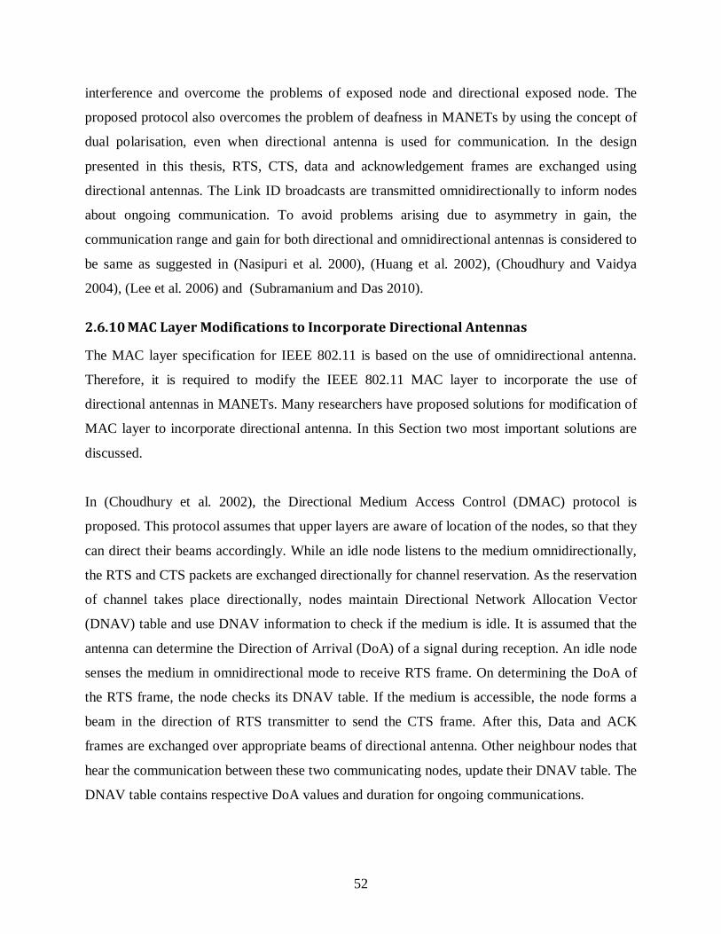
52

interference and overcome the problems of exposed node and directional exposed node. The

proposed protocol also overcomes the problem of deafness in MANETs by using the concept of

dual polarisation, even when directional antenna is used for communication. In the design

presented in this thesis, RTS, CTS, data and acknowledgement frames are exchanged using

directional antennas. The Link ID broadcasts are transmitted omnidirectionally to inform nodes

about ongoing communication. To avoid problems arising due to asymmetry in gain, the

communication range and gain for both directional and omnidirectional antennas is considered to

be same as suggested in (Nasipuri et al. 2000), (Huang et al. 2002), (Choudhury and Vaidya

2004), (Lee et al. 2006) and (Subramanium and Das 2010).

2.6.10 MAC Layer Modifications to Incorporate Directional Antennas

The MAC layer specification for IEEE 802.11 is based on the use of omnidirectional antenna.

Therefore, it is required to modify the IEEE 802.11 MAC layer to incorporate the use of

directional antennas in MANETs. Many researchers have proposed solutions for modification of

MAC layer to incorporate directional antenna. In this Section two most important solutions are

discussed.

In (Choudhury et al. 2002), the Directional Medium Access Control (DMAC) protocol is

proposed. This protocol assumes that upper layers are aware of location of the nodes, so that they

can direct their beams accordingly. While an idle node listens to the medium omnidirectionally,

the RTS and CTS packets are exchanged directionally for channel reservation. As the reservation

of channel takes place directionally, nodes maintain Directional Network Allocation Vector

(DNAV) table and use DNAV information to check if the medium is idle. It is assumed that the

antenna can determine the Direction of Arrival (DoA) of a signal during reception. An idle node

senses the medium in omnidirectional mode to receive RTS frame. On determining the DoA of

the RTS frame, the node checks its DNAV table. If the medium is accessible, the node forms a

beam in the direction of RTS transmitter to send the CTS frame. After this, Data and ACK

frames are exchanged over appropriate beams of directional antenna. Other neighbour nodes that

hear the communication between these two communicating nodes, update their DNAV table. The

DNAV table contains respective DoA values and duration for ongoing communications.

53

Directional Virtual Carrier Sensing (DVCS) mechanism is proposed in (Takai et al. 2002). This

mechanism is composed of mainly three functionalities: Angle of Arrival (AoA) caching, beam

locking and unlocking, and DNAV. During AoA caching, all the nodes maintain AoA cache for

their neighbour nodes whenever they detect any signal from the neighbour nodes. For beam

locking, when a node receives the RTS frame from its neighbour, it adapts its beam pattern to

achieve maximum received power. It locks the beam pattern to transmit CTS to the node. On

receiving CTS, the RTS transmitter also locks its beam in the appropriate direction. On the

completion of communication, these beam patterns are unlocked. While the communication

between two nodes takes place, other nodes use DNAV to maintain the NAV timer. Using this

DNAV timer, other nodes in the network check the completion of ongoing communication and

access the medium accordingly.

2.7 Network Layer in MANETs

One of the primary tasks carried out by the network layer in MANETs is routing. Due to

dynamic nature and absence of infrastructure, routing plays an important role in the operation of

MANETs. Extensive research has been carried out in this area, and many routing protocols have

been proposed for the same. This section discusses different approaches and design choices for

development of routing protocols, and significance of multipath routing in MANETs.

While developing the routing protocols for MANETs, it is essential to keep the characteristics of

MANETs in consideration. Some of the main characteristics that must be considered while

designing a routing protocol for MANETs are as explained below (Belding-Royer 2004):

Multihop routing: As all the nodes in MANET need to participate in routing of information due

to absence of any infrastructure, the designed routing protocol must be capable of discovering

multihop paths between source and destination nodes.

Less processing and control overhead: The participating nodes may have limited battery

energy and computational resources. Also, wireless medium has limited bandwidth. Therefore, it

is required that the computational complexity of the designed protocol should be less and only

necessary control packets are exchanged between the nodes for establishment and maintenance

of routes.

54

Node mobility maintenance: As MANETs are established from mobile nodes, network

topology may constantly keep changing. The designed protocol must consider the change in

network topology. Based on this, the protocol can be designed to either establish routes only on

demand or by constantly exchanging routing table updates.

Loop-free routing: While establishing the route from a source to destination, it is very

important that loop-free routes are established between the nodes. Loop-free routing ensures that

a node does not occur in the established path multiple times. In case a loop is present in the

established path, the packets traverse the path multiple times and may get dropped without

reaching the destination, if the Time-To-Live (TTL) value reaches zero. With limited available

bandwidth of wireless medium, such packets lead to congestion of network and deterioration of

network performance.

Minimum latency: Time taken for establishment of routes and their recovery due to broken

routes must be low. Lack of these capabilities can lead to packet drops and time delays in

arriving at the destination.

2.7.1 Different Approaches of Routing in MANETs

While there are different approaches for routing in MANETs, principal approaches are Proactive,

Reactive and Hybrid routing. Proactive routing protocols are also known as Table-driven routing

protocols as the nodes using such protocols maintain latest routes to different destinations by

periodically exchanging routing tables with other nodes in the network. Reactive routing

protocols are also known as on-demand routing protocols as the nodes using these protocols

initiate discovery and establishment of routes only when required. Hybrid routing protocols are a

combination of reactive and proactive approaches. In this section, these routing approaches, their

advantages and disadvantages are discussed in detail.

Proactive Routing: As the name suggests, nodes using proactive routing protocols maintain

routing tables, whether there is any data to exchange or not. The nodes constantly exchange

routing table updates with their neighbour nodes according to predefined periods and maintain

55

routes to other nodes in the network. Due to the characteristic of exchanging routing tables

periodically to maintain the routes, these protocols are also named as table-driven routing

protocols. As the routes are always available, whenever the application layer of source node

needs to transmit data to a destination node, the network layer selects appropriate route to the

destination node from source node. Therefore, there is negligible delay in route establishment

and data transfer from node to the medium. Some of the examples of proactive routing protocols

are Clusterhead Gateway Switch Routing (CGSR) (Chiang et al. 1997), Destination Sequenced

Distance Vector (DSDV) (Perkins and Bhagwat 1994), and Optimised Link State Routing

(OLSR) (Jacquet et al. 2001).

As proactive routing protocols constantly exchange routing tables and maintain latest routes,

latency in route establishment is negligible. However, as the nodes participating in the network

are mobile, established routes may become invalid frequently. This can lead to frequent

exchange of routing updates among the nodes, leading to increased control overhead in the

network. Such frequent exchanges of control packets also lead to early exhaustion of limited

battery power available with the nodes. Therefore, use of proactive routing protocols is preferred

in the networks where nodes are either stationary or less mobile, in order to avoid route updates.

Proactive routing protocols are also preferred to be used for low latency applications over

MANETs to overcome the delay for route establishment (Belding-Royer 2004).

Reactive Routing: Unlike proactive routing protocols, nodes using reactive routing protocols

carry out discovery and establishment of routes only when data exchange needs to take place.

Therefore, with reactive protocols, nodes do not need to exchange periodic routing updates. Due

to this characteristic of initiating route discovery only when required, these protocols are also

known as on-demand routing protocols. As establishment of routes starts only when data needs

to be exchanged, delay is experienced between the time the data is ready at the application layer

and by the time it is transmitted to the medium by lower layers. For route discovery, network is

flooded with route request packets by the source and intermediate nodes till the route request

packet reaches the required destination. On receiving the route request packet, destination node

sends route reply to the original source through the intermediate nodes. Some of the examples of

reactive routing protocols are Ad-hoc On-demand Distance Vector routing (AODV) (Perkins,

56

Belding-Royer and Das 2003), Dynamic Source Routing (DSR) (Johnson, Maltz and Broch

2001) and Temporally-Ordered Routing Algorithm (TORA) (Park and Corson 1997).

As reactive protocols do not require exchange of periodic route updates, number of control

packets transmitted by the nodes is much lesser when compared to proactive routing protocols.

This helps in reducing protocol overhead and therefore achieving efficient use of available

bandwidth. Absence of periodic exchange of routing updates also reduces the consumption of

limited battery power available with the nodes. As route discovery is initiated only when

required, there are less instances of routes becoming stale due to mobility of nodes. However,

excessive flooding of route request packets can lead to network congestion. To avoid this, many

reactive routing protocols use controlled flooding wherein, if an intermediate node has already

forwarded a route request packet, it will not forward it again. All these characteristics make

reactive protocols useful for applications which do not particularly require low latency (Belding-

Royer 2004).

Hybrid Routing: Hybrid routing combines the advantages of both reactive and proactive routing

protocols. These protocols help in achieving higher scalability of network wherein, the nodes in

close proximity are capable of working together to reduce the overhead in route discovery.

Hybrid routing protocols generally use location information of nodes for routing of information.

Routes to nearby or neighbour nodes are established proactively, while routes to nodes located

far away from the source are discovered reactively. Some of the hybrid routing protocols are

Zone Routing Protocol (ZRP) (Haas, Pearlman and Samar2002), Zone-based Hierarchical Link

State (ZHLS) (Joa-Ng and Lu 1999) and Distributed Dynamic Routing (DDR) (Nikaein, Labiod

and Bonnet 2000).

As hybrid routing protocols combine the advantages of both proactive and reactive routing

protocols, they are capable of achieving higher efficiency and scalability of network when

compared to only proactive or only reactive approaches. In hybrid protocols, number of

rebroadcasting nodes is reduced as all the nodes already form neighbour tables by virtue of

mechanism of proactive routing. Therefore, only far off nodes need to be discovered using route

request broadcasts in accordance with mechanism of reactive routing. Also, nodes with highly

57

populated neighbour tables serve as the most suitable nodes for route discovery. Hybrid routing

protocols are generally preferred for most of the applications, as they offer advantages of both

reactive and proactive routing protocols (Belding-Royer 2004).

2.7.2 Multipath Routing in MANETs

Multipath routing involves establishment of multiple paths/routes between the source and

destination nodes. Most of the routing protocols discover only single path from a particular

source node to required destination node. While the route discovery process adopted by these

protocols is simple, in case the established route breaks or becomes non-functional, re-discovery

of routes needs to be initiated. Instead of this, if the routing protocol is designed such that it

discovers multiple paths from source to destination nodes, there will always be backup routes

available in case one route breaks. For this, nodes maintain a route cache with multiple route

entries for a particular destination node. The source node may either use all the paths

simultaneously to carry out load sharing or may use the best path out of all the discovered paths

as primary path. Therefore, in case the primary path breaks, source node can use other available

paths for routing of information to the destination node (Lee and Gerla 2000). Benefits of

multipath routing are as follows:

1. Robustness and reliability: As the source node maintains multiple paths to the

destination, in case one path breaks due to dynamic nature of MANETs, other backup

paths can be considered for data transmission without hindering the ongoing

communication. This helps in achieving robust and reliable data communication in the

network (Lee and Gerla 2000)

2. Load sharing: With multiple available paths, a source node can use all the paths

simultaneously for transmission of data to the destination. Multiple streams of data can be

transmitted over different paths simultaneously. This avoids overloading of nodes in

single path and drop of data due to congestion in one path (Mueller, Tsang and Ghosal

2004)

3. Increased aggregate bandwidth: As wireless networks have limited bandwidth, data

transmission over single path may not achieve efficient use of available bandwidth. By

58

transmitting data over multiple paths simultaneously, nodes get benefitted from increased

aggregate bandwidth which enhances performance of network (Mueller, Tsang and

Ghosal 2004)

4. Reduced end-to-end delay: With parallel data transmission over multiple paths, the time

taken by data packets at source node to reach the destination, also termed as latency or

end-to-end delay reduces drastically. Reduced end-to-end delay increases the efficiency

and performance of the network (Mueller, Tsang and Ghosal 2004)

5. Reduced energy consumption: By sharing the network traffic load among different

nodes which are part of different paths between source and destination nodes, it is

ensured that particular set of nodes belonging to the best path do not get overloaded. If

the nodes get overloaded, they tend to exhaust their battery energy faster. Such nodes

lead to reduced lifetime of the overall network. Multipath routing enhances the network

lifetime by ensuring that traffic load is distributed among multiple nodes in the network

(Mueller, Tsang and Ghosal 2004)

While there are many advantages of multipath routing, it is associated with certain challenges

which are listed below:

1. Complex route discovery: The process of route discovery and maintenance in multipath

routing is complex when compared to that in unipath routing as it is required to discover

multiple loop free paths between the nodes (Belding-Royer 2004). Many protocols also

prefer the discovered paths to be node-disjoint or link-disjoint as explained in Section6.4

of Chapter 6, which further adds to the complexity of route discovery procedure

(Meghanathan 2010)

2. Interference among multiple paths: While multipath routing gives freedom to carry out

parallel data transmission over different paths, it can lead to interference between

transmissions on adjacent paths. This can cause degradation of network performance by

limiting the maximum achievable throughput (Saha et al. 2003) and (Waharte and

Boutaba 2006)

59

2.7.3 Different Types of Multipath Routes

Multipath routes can be mainly of four types:

1. Node-disjoint: Node-disjoint routes are the ones which have no nodes in common, other

than the source and destination nodes. Therefore, in case of node failure only the route

comprising that particular node gets affected, while other routes still remain functional.

Node-disjoint routes are also known as totally disjoint routes, and provide highest degree

of fault tolerance. These routes present the maximum aggregate resources, because

neither nodes nor links are shared among different paths. However, in a sparse network,

as the inter-node distance increases, it becomes difficult to discover node-disjoint routes

(Waharte and Boutaba 2006). An example of node-disjoint routes is shown in Figure

6-10of Chapter 6. It can be seen from Figure 6-10that none of the nodes (other than the

source and destination nodes) in available multiple paths are common. Examples of node-

disjoint routing protocols are AODV Multipath (AODVM) (Ye, Krishnamurthy and

Tripathi 2003) and Energy aware Multipath Routing Protocol (EMRP) (Li et al. 2005)

2. Link-disjoint: Link-disjoint routes are the ones which may have common nodes, but do

not have common links. As link-disjoint routes may share common nodes, failure of one

node affects all the routes which have this node in common. When compared to node-

disjoint routes, link-disjoint routes provide lesser aggregate resources due to the presence

of common nodes between different routes. Common nodes in different routes need to

operate for longer duration and handle higher load when compared to other nodes. This

leads to higher energy consumption of nodes, increasing the chances of node failure

leading to failure of multiple routes (Meghanathan 2010). Examples of link-disjoint

routes are Split Multipath Routing (SMR) protocol (Lee and Gerla 2001) and Ad-hoc On

demand Multipath Distance Vector (AOMDV) routing protocol (Marina and Das

2001).An example of link-disjoint routes is shown in Figure 6-11 of Chapter 6

3. Non-disjoint: Non-disjoint routes share common nodes and links. Therefore, in case

these common nodes or links between multiple routes fail, all the associated routes stop

functioning. Due to this, non-disjoint routes provide least aggregate resources and fault-

tolerance, when compared to node-disjoint or link-disjoint routes. It has been observed in

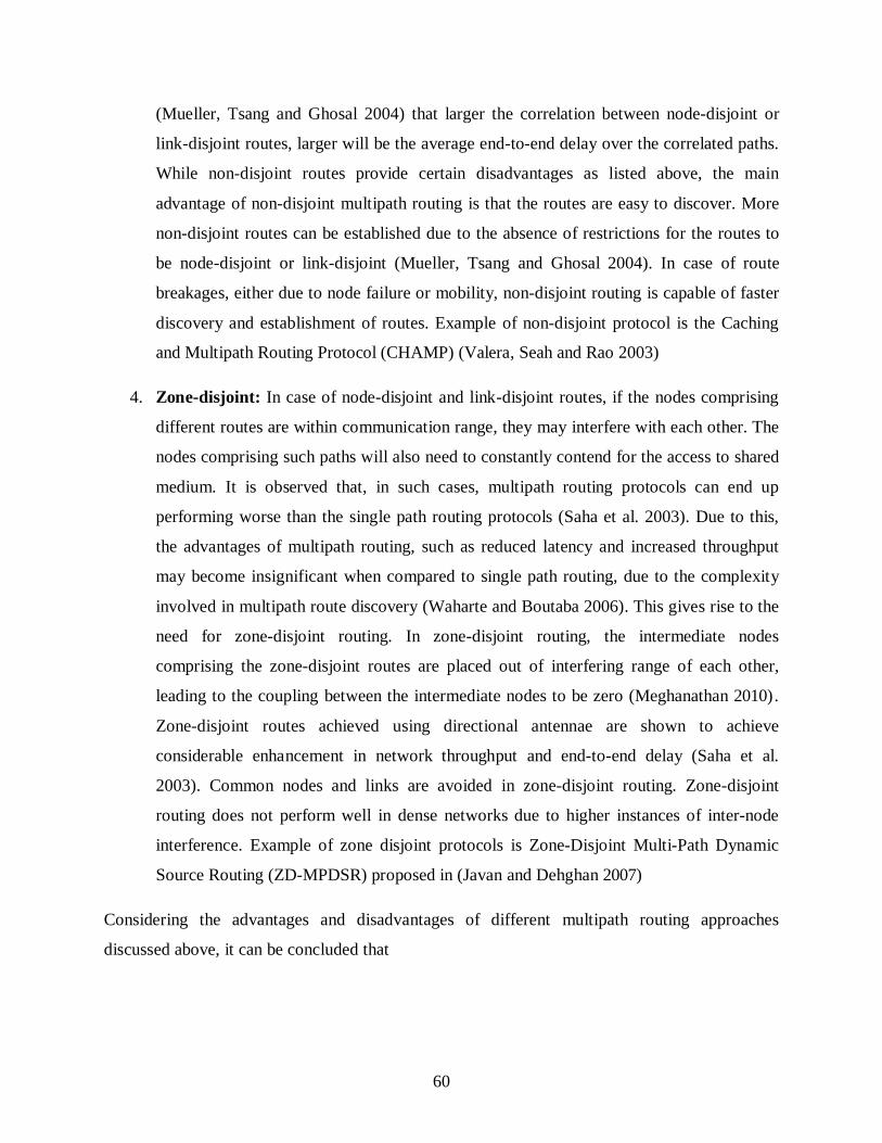
60

(Mueller, Tsang and Ghosal 2004) that larger the correlation between node-disjoint or

link-disjoint routes, larger will be the average end-to-end delay over the correlated paths.

While non-disjoint routes provide certain disadvantages as listed above, the main

advantage of non-disjoint multipath routing is that the routes are easy to discover. More

non-disjoint routes can be established due to the absence of restrictions for the routes to

be node-disjoint or link-disjoint (Mueller, Tsang and Ghosal 2004). In case of route

breakages, either due to node failure or mobility, non-disjoint routing is capable of faster

discovery and establishment of routes. Example of non-disjoint protocol is the Caching

and Multipath Routing Protocol (CHAMP) (Valera, Seah and Rao 2003)

4. Zone-disjoint: In case of node-disjoint and link-disjoint routes, if the nodes comprising

different routes are within communication range, they may interfere with each other. The

nodes comprising such paths will also need to constantly contend for the access to shared

medium. It is observed that, in such cases, multipath routing protocols can end up

performing worse than the single path routing protocols (Saha et al. 2003). Due to this,

the advantages of multipath routing, such as reduced latency and increased throughput

may become insignificant when compared to single path routing, due to the complexity

involved in multipath route discovery (Waharte and Boutaba 2006). This gives rise to the

need for zone-disjoint routing. In zone-disjoint routing, the intermediate nodes

comprising the zone-disjoint routes are placed out of interfering range of each other,

leading to the coupling between the intermediate nodes to be zero (Meghanathan 2010).

Zone-disjoint routes achieved using directional antennae are shown to achieve

considerable enhancement in network throughput and end-to-end delay (Saha et al.

2003). Common nodes and links are avoided in zone-disjoint routing. Zone-disjoint

routing does not perform well in dense networks due to higher instances of inter-node

interference. Example of zone disjoint protocols is Zone-Disjoint Multi-Path Dynamic

Source Routing (ZD-MPDSR) proposed in (Javan and Dehghan 2007)

Considering the advantages and disadvantages of different multipath routing approaches

discussed above, it can be concluded that

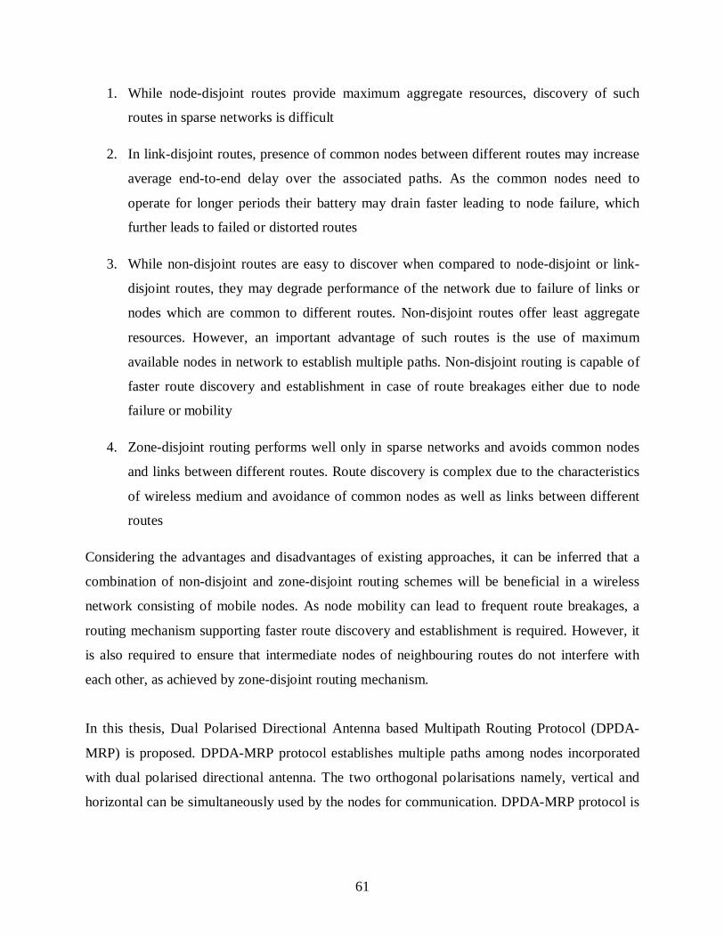
61

1. While node-disjoint routes provide maximum aggregate resources, discovery of such

routes in sparse networks is difficult

2. In link-disjoint routes, presence of common nodes between different routes may increase

average end-to-end delay over the associated paths. As the common nodes need to

operate for longer periods their battery may drain faster leading to node failure, which

further leads to failed or distorted routes

3. While non-disjoint routes are easy to discover when compared to node-disjoint or link-

disjoint routes, they may degrade performance of the network due to failure of links or

nodes which are common to different routes. Non-disjoint routes offer least aggregate

resources. However, an important advantage of such routes is the use of maximum

available nodes in network to establish multiple paths. Non-disjoint routing is capable of

faster route discovery and establishment in case of route breakages either due to node

failure or mobility

4. Zone-disjoint routing performs well only in sparse networks and avoids common nodes

and links between different routes. Route discovery is complex due to the characteristics

of wireless medium and avoidance of common nodes as well as links between different

routes

Considering the advantages and disadvantages of existing approaches, it can be inferred that a

combination of non-disjoint and zone-disjoint routing schemes will be beneficial in a wireless

network consisting of mobile nodes. As node mobility can lead to frequent route breakages, a

routing mechanism supporting faster route discovery and establishment is required. However, it

is also required to ensure that intermediate nodes of neighbouring routes do not interfere with

each other, as achieved by zone-disjoint routing mechanism.

In this thesis, Dual Polarised Directional Antenna based Multipath Routing Protocol (DPDA-

MRP) is proposed. DPDA-MRP protocol establishes multiple paths among nodes incorporated

with dual polarised directional antenna. The two orthogonal polarisations namely, vertical and

horizontal can be simultaneously used by the nodes for communication. DPDA-MRP protocol is

62

a combination of non-disjoint and zone-disjoint routing mechanisms, which is explained in

Chapter 6.

2.8 Vehicular Ad-Hoc Networks (VANETs)

Vehicular Ad hoc Networks (VANETs) are a subclass of MANETs, wherein, vehicles are the

mobile nodes forming a network. Both MANETs and VANETs are characterised by movement

and self-organisation of the participating nodes. However, the characteristics exhibited by

VANETs are different from those of MANETs. While MANETs are formed by nodes having un-

controlled or random mobility patterns, VANETs are formed by vehicles whose movements are

restricted due to factors such as traffic, traffic regulations and road course (Yousefi, Mousavi and

Fathy 2006) and (Li and Wang 2007). Apart from the difference in mobility patterns, the

MANETs and VANETs also vary in communication protocol. While communication between

nodes in MANETs is based on IEEE 802.11 a/b/g standards (Burton 2009) and their

enhancements, the nodes in VANETs are required to communicate based on the North

American, Dedicated Short Range Communication (DSRC) standard which uses IEEE 802.11p

standard to enable wireless communication between the nodes (Yousefi, Mousavi and Fathy

2006). Also, unlike the nodes in MANETs, the nodes in VANETs (vehicles) are not subjected to

energy constraints and restrictions in computing capabilities (Fiore et al. 2007) and (Yousefi,

Mousavi and Fathy 2006).

The critical aspect of simulation study of VANETs is the need for mobility models and road

topologies that can simulate real behaviour of vehicular traffic (Fiore et al. 2007). Hence, mere

increasing the speed of MANET nodes to match vehicular speeds will not be sufficient to study

the performance of VANETs. Therefore, this thesis concentrates on simulation studies of

MANETs alone, to simulate walking and running speed of humans having random mobility

patterns. While the proposed dual polarised directional antenna based communication can be

applied to VANETs as well, the simulation study of VANETs will require different mobility

models, road topologies and communication standard. In future, the study of performance of the

proposed dual polarised directional antenna based communication can be extended to VANETs.

63

2.9 Conclusion

This chapter is aimed to present an introduction to MANETs, their characteristics, challenges,

brief review of available methods in literature to overcome these challenges and their limitations.

Three layers of network protocol stack, that play significant role in the operation and

performance of MANETs are the physical, MAC and network layers.

Physical layer in MANETs is responsible for transmission and reception of signals exchanged

between the nodes communicating over wireless medium. Different ranges in wireless medium

under which nodes may fall such as transmission, carrier sensing and interference ranges are

discussed, along with the importance of power control, to avoid interference as well as link

outage. The concept of threshold SNR and its importance in identifying whether the nodes fall

within transmission, carrier sensing or interference range of each other are explained in detail.

Physical layer deals with different types of antennas used for communication and their

characteristics. In this chapter, characteristics of omnidirectional and directional antennas are

presented. Among directional antennas, switched beam and steered beam antennas are

considered for study. Antenna characteristics such as gain of antenna, radiation pattern,

beamwidth, directivity and polarisation of the antenna are discussed in detail. Benefits of

directional communication and power control in MANETs are also covered in this chapter.

Present schemes for avoidance of interference among the nodes in MANETs by using directional

antenna and power control are also discussed. Many researchers have appreciated the role of

antenna polarisation and directional communication for avoidance of interference in MANETs.

This chapter clearly distinguishes the role of dual polarised directional antenna in MANETs, vis-

a-vis its current utility in polarisation diversity.

Method used for access to the medium plays a significant role in deciding performance of the

network. The existing IEEE 802.11 based CSMA/CA protocol used in MANETs for controlling

access to the medium is explained and problems such as hidden nodes, exposed nodes and

deafness are discussed in detail. Directional antennas help in overcoming the problem of exposed

nodes in MANETs. However, use of directional antenna requires changes in existing IEEE

802.11 based CSMA/CA mechanism. The current schemes for modifications to MAC layer to

incorporate directional antennas are discussed. While use of directional antenna helps in

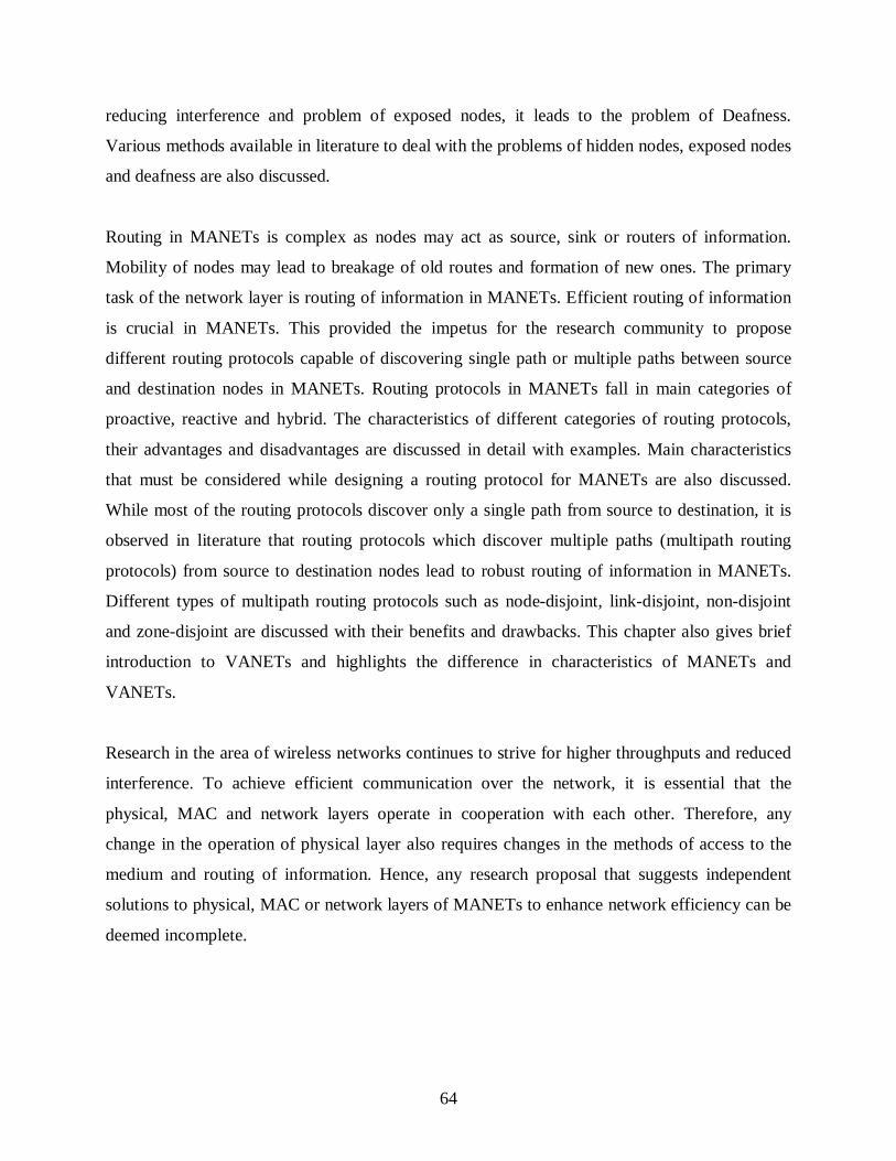
64

reducing interference and problem of exposed nodes, it leads to the problem of Deafness.

Various methods available in literature to deal with the problems of hidden nodes, exposed nodes

and deafness are also discussed.

Routing in MANETs is complex as nodes may act as source, sink or routers of information.

Mobility of nodes may lead to breakage of old routes and formation of new ones. The primary

task of the network layer is routing of information in MANETs. Efficient routing of information

is crucial in MANETs. This provided the impetus for the research community to propose

different routing protocols capable of discovering single path or multiple paths between source

and destination nodes in MANETs. Routing protocols in MANETs fall in main categories of

proactive, reactive and hybrid. The characteristics of different categories of routing protocols,

their advantages and disadvantages are discussed in detail with examples. Main characteristics

that must be considered while designing a routing protocol for MANETs are also discussed.

While most of the routing protocols discover only a single path from source to destination, it is

observed in literature that routing protocols which discover multiple paths (multipath routing

protocols) from source to destination nodes lead to robust routing of information in MANETs.

Different types of multipath routing protocols such as node-disjoint, link-disjoint, non-disjoint

and zone-disjoint are discussed with their benefits and drawbacks. This chapter also gives brief

introduction to VANETs and highlights the difference in characteristics of MANETs and

VANETs.

Research in the area of wireless networks continues to strive for higher throughputs and reduced

interference. To achieve efficient communication over the network, it is essential that the

physical, MAC and network layers operate in cooperation with each other. Therefore, any

change in the operation of physical layer also requires changes in the methods of access to the

medium and routing of information. Hence, any research proposal that suggests independent

solutions to physical, MAC or network layers of MANETs to enhance network efficiency can be

deemed incomplete.

65

CHAPTER 3

3 Mitigation of Interference through Dual Polarisation

3.1 Introduction

As the wireless medium is unguarded, simultaneous occurrence of transmissions between nodes

may lead to interference. Interference between the nodes increases with increase in density of

nodes in the network. Inter-node interference leads to corruption of data, which further leads to

drop of packets at the receivers resulting in deterioration of overall performance of the network.

MANETs operate in 2.4 GHz frequency band which is an Industrial, Scientific and Medical

(ISM) band permitted for unlicensed operation. As the ISM band is allocated for unlicensed

operations, interference experienced in such bands is high due to large number of devices

accessing the medium for communication (Chiasserini and Rao 2003) and (Sikora and Groza

2005). Therefore, it becomes essential to utilise methods and techniques that can help in

mitigation of interference, thus enhancing the performance of the network.

This chapter presents the benefits of using dual polarised directional communication to mitigate

interference among nodes present in MANET. Use of directional communication over

orthogonal polarisations helps in achieving increased spatial reuse, thus allowing multiple nodes

to carry out simultaneous communication without interference. Through the simulations carried

out using Qualnet simulator, it is shown that spatial reuse achieved through the use of dual

polarised directional communication helps in reducing inter-node interference and increasing the

performance of the network.

3.2 Interference in Wireless Networks

As studied in Section 2.5.3 of Chapter 2, the nodes in a wireless network fall within three

different ranges of each other, namely, interference range, carrier sensing range and transmission

range. When two nodes are within the interference range of each other, they deteriorate each

other’s signals, leading to degradation in network performance. Due to mobility of nodes,

interference conditions between nodes of MANET change constantly.

66

Interference due to other nodes in the network is measured at the receiver node. The relation

given in Equation 2.17, of Chapter 2 is used to measure interference range for omnidirectional

(Xu, Gerla and Bae 2003) and directional (Hong-Ning et al., 2008) communication. For

MANETs, the threshold SNR (TSNR) is usually considered to be 10 dB (Xu, Gerla and Bae

2003). For two-ray ground model value of the constant k is 4 (Xu, Gerla and Bae 2003). The

nodes communicating over IEEE 802.11 based MANETs can communicate up to a distance of

250 m or above (Bazan and Jaseemuddin 2011), (Subramanian and Das 2010), (Meghanathan

2010), (Durvy, Dousse and Thiran 2007), (Vassis and Kormentzas 2006), (Seo et al. 2005),

(Choudhury and Vaidya 2004),(Tang and Gerla 2000) and (USRobotics Technical Report).

However, for dual polarised communication, channel orthogonality is maintained for a maximum

distance of 200 m only, in Line Of Sight (LOS) settings for ad-hoc networks (Khalid et al. 2011).

Therefore, for the proposed dual polarised directional communication, the maximum

communication distance chosen for simulations is 200 m.

With value of 𝑇𝑇𝐿𝐿𝑆𝑆𝑅𝑅 = 10 dB and 𝑘𝑘 = 4 (for two-ray ground model) and 𝑑𝑑 = 200 m for IEEE

802.11 based wireless networks, the interference range can be calculated as given in Equation

3.1

𝑅𝑅𝑑𝑑 = √104 × 200 = 1.778 × 200 = 355.65 ...3.1

Therefore, to receive signals with value of SNR above threshold, it is required that the distance

between intended receiver and interferer nodes should be greater than 355.65 m. If the intended

receiver and interferer nodes are located closer than 355.65 m, then the SNR of the received

signal is below threshold SNR and the received signal is discarded. This leads to degradation in

network performance and waste of network bandwidth.

The variation in network performance, by varying the distance between receiver and interferer

nodes is studied through simulations in Qualnet. The scenario shown in Figure 3-1has two pairs

of communicating nodes. The scenario is developed based on specifications given in Table 3-1.

For two pairs of communicating nodes 4 nodes are used in the scenario. As observed from the

scenario, Nodes 1 and 2 communicate, with Node 1 being the transmitter and Node 2 the

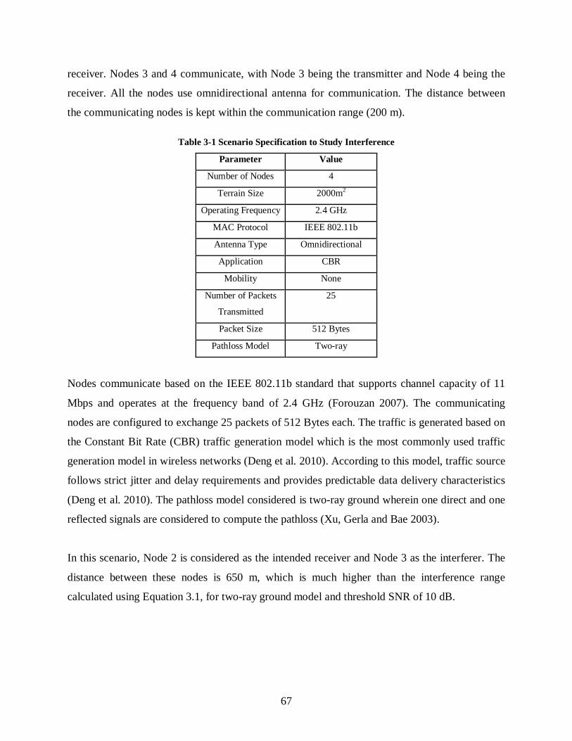
67

receiver. Nodes 3 and 4 communicate, with Node 3 being the transmitter and Node 4 being the

receiver. All the nodes use omnidirectional antenna for communication. The distance between

the communicating nodes is kept within the communication range (200 m).

Table 3-1 Scenario Specification to Study Interference

Parameter Value

Number of Nodes 4

Terrain Size 2000m2

Operating Frequency 2.4 GHz

MAC Protocol IEEE 802.11b

Antenna Type Omnidirectional

Application CBR

Mobility None

Number of Packets

Transmitted

25

Packet Size 512 Bytes

Pathloss Model Two-ray

Nodes communicate based on the IEEE 802.11b standard that supports channel capacity of 11

Mbps and operates at the frequency band of 2.4 GHz (Forouzan 2007). The communicating

nodes are configured to exchange 25 packets of 512 Bytes each. The traffic is generated based on

the Constant Bit Rate (CBR) traffic generation model which is the most commonly used traffic

generation model in wireless networks (Deng et al. 2010). According to this model, traffic source

follows strict jitter and delay requirements and provides predictable data delivery characteristics

(Deng et al. 2010). The pathloss model considered is two-ray ground wherein one direct and one

reflected signals are considered to compute the pathloss (Xu, Gerla and Bae 2003).

In this scenario, Node 2 is considered as the intended receiver and Node 3 as the interferer. The

distance between these nodes is 650 m, which is much higher than the interference range

calculated using Equation 3.1, for two-ray ground model and threshold SNR of 10 dB.

68

Figure 3-1 Scenario with Non-Interfering Nodes

The results obtained at the physical layer for the same scenario are presented in Figure 3-2. From

the obtained results shown in Figure 3-2, it is observed that Nodes 2 and 4, which are receivers

for both the communication pairs receive equal number of signals at the physical layer.

(a) Signals received at Nodes 2 and 4 (b) Signals received with errors

Figure 3-2 Signal at Physical Layer with Non-Interfering Nodes

This denotes that all the signals arrived at the physical layer are above the threshold SNR of 10

dB and none of the signals arriving at any of the two receivers (Nodes 2 and 4) are erroneous.

While Nodes 1 and 3 are transmitters, it is observed that received signals are present at these

nodes also (Figure 3-2 a), though number of signals received at Nodes 1 and 3 are much smaller

than the number of signals received by the receivers. Received signals are present at transmitting

nodes also because in Qualnet, the communicating nodes exchange certain control signals such

as MAC control signals or periodic heartbeat signals, which are received by both transmitting

and receiving nodes.

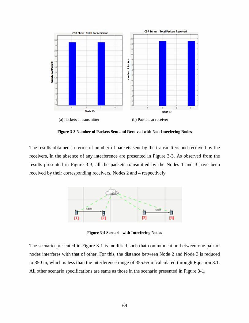
69

(a) Packets at transmitter (b) Packets at receiver

Figure 3-3 Number of Packets Sent and Received with Non-Interfering Nodes

The results obtained in terms of number of packets sent by the transmitters and received by the

receivers, in the absence of any interference are presented in Figure 3-3. As observed from the

results presented in Figure 3-3, all the packets transmitted by the Nodes 1 and 3 have been

received by their corresponding receivers, Nodes 2 and 4 respectively.

Figure 3-4 Scenario with Interfering Nodes

The scenario presented in Figure 3-1 is modified such that communication between one pair of

nodes interferes with that of other. For this, the distance between Node 2 and Node 3 is reduced

to 350 m, which is less than the interference range of 355.65 m calculated through Equation 3.1.

All other scenario specifications are same as those in the scenario presented in Figure 3-1.

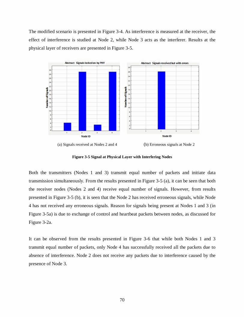
70

The modified scenario is presented in Figure 3-4. As interference is measured at the receiver, the

effect of interference is studied at Node 2, while Node 3 acts as the interferer. Results at the

physical layer of receivers are presented in Figure 3-5.

(a) Signals received at Nodes 2 and 4 (b) Erroneous signals at Node 2

Figure 3-5 Signal at Physical Layer with Interfering Nodes

Both the transmitters (Nodes 1 and 3) transmit equal number of packets and initiate data

transmission simultaneously. From the results presented in Figure 3-5 (a), it can be seen that both

the receiver nodes (Nodes 2 and 4) receive equal number of signals. However, from results

presented in Figure 3-5 (b), it is seen that the Node 2 has received erroneous signals, while Node

4 has not received any erroneous signals. Reason for signals being present at Nodes 1 and 3 (in

Figure 3-5a) is due to exchange of control and heartbeat packets between nodes, as discussed for

Figure 3-2a.

It can be observed from the results presented in Figure 3-6 that while both Nodes 1 and 3

transmit equal number of packets, only Node 4 has successfully received all the packets due to

absence of interference. Node 2 does not receive any packets due to interference caused by the

presence of Node 3.

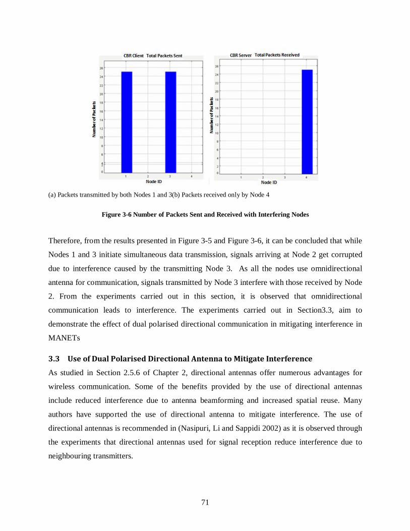
71

(a) Packets transmitted by both Nodes 1 and 3(b) Packets received only by Node 4

Figure 3-6 Number of Packets Sent and Received with Interfering Nodes

Therefore, from the results presented in Figure 3-5 and Figure 3-6, it can be concluded that while

Nodes 1 and 3 initiate simultaneous data transmission, signals arriving at Node 2 get corrupted

due to interference caused by the transmitting Node 3. As all the nodes use omnidirectional

antenna for communication, signals transmitted by Node 3 interfere with those received by Node

2. From the experiments carried out in this section, it is observed that omnidirectional

communication leads to interference. The experiments carried out in Section3.3, aim to

demonstrate the effect of dual polarised directional communication in mitigating interference in

MANETs

3.3 Use of Dual Polarised Directional Antenna to Mitigate Interference

As studied in Section 2.5.6 of Chapter 2, directional antennas offer numerous advantages for

wireless communication. Some of the benefits provided by the use of directional antennas

include reduced interference due to antenna beamforming and increased spatial reuse. Many

authors have supported the use of directional antenna to mitigate interference. The use of

directional antennas is recommended in (Nasipuri, Li and Sappidi 2002) as it is observed through

the experiments that directional antennas used for signal reception reduce interference due to

neighbouring transmitters.

72

While directional antennas can enhance network performance by reducing interference, the

performance of the network can be improved further by exploiting the polarisation characteristic

of an antenna. As studied in Section 2.5.5 of Chapter 2,antenna typically generates

electromagnetic waves with the electric field oriented either parallel or perpendicular to the

direction of propagation. These are called as horizontally or vertically polarised waves

respectively. The electromagnetic waves in these polarisations are orthogonal to each other. If

two pairs of neighbouring nodes communicate using directional antennas with orthogonal

polarisations, interference between the two communication links can be avoided, thus enabling

simultaneous communication among two pairs of neighbouring nodes, without interference. The

communication links using two orthogonal polarisations can be considered as two independent

channels which can be used for exchange of data simultaneously, without interference. This

helps in enhancing the performance and efficiency of the network. Signals transmitted over

wireless medium undergo reflection, refraction, scattering, and diffraction, leading to

depolarisation. However, as stated in (Khalid et al. 2011), in Line of Sight (LoS) settings in

wireless networks, channel orthogonality is maintained for distances of up to 50m-200m. Use of

dual polarised antennas for data communication in wireless networks is documented in (Yildirim

and Liu 2007) and (Khalid et al. 2011). The methods proposed in these papers use polarisation

diversity for enhancing network performance.

In this thesis, the concept of dual polarisation is proposed, wherein, a node can either use single

polarisation at a time or simultaneously use two orthogonal polarisations for communication.

This helps in reducing deterioration of signal due to interference while providing two

simultaneous non-interfering channels for nodes to communicate. In this section, the effect of

dual polarised directional antennas in mitigating interference is studied and analysed through

simulations in Qualnet simulator. Qualnet offers two types of directional antenna

implementations; one is a steerable directional antenna and other is that of a switched beam

antenna. In this study, the switched beam antenna is used. The switched beam antenna

implemented in Qualnet is composed of eight directional beams covering 360o as shown in

Figure 3-7. Based on the location of receiver, the transmitter chooses the appropriate beam

pointing in the direction of the receiver.

73

However, at a time a node can use only one directional beam pointing towards the receiver.

Based on this implementation of switched beam directional antenna, the scenarios are developed

to study the effect of dual polarised directional antennas on interference in ad-hoc networks.

Figure 3-7 Orientation of Switched Beams in Qualnet

The scenario presented in Figure 3-8 consists of 32 nodes with directional beams for

communication. In all, there are 16 communication links distributed equally along 8 beams of the

switched beam antenna. Along each directional beam, there are two communication links. As the

switched beam antenna implementation in Qualnet has eight beams, Nodes 9, 17, 1, 29, 13, 25, 5

and 21 use directional beams numbered 0, 1, 2, 3, 4, 5, 6 and 7 respectively to communicate with

their respective receivers.

The beam numbers marked in Figure 3-8 show the beam orientation of the transmitters for

corresponding communication links. Therefore, the link marked ‘Beam 0’ states that the

directional beams of transmitters (Nodes 9 and 11) are directed along beam 0. Same explanation

holds good for other beam numbers over other communication links also. In Figure 3-8, the two

transmitting nodes with their directional antennas oriented along beam 0 are Nodes 9 and

11.Nodes 9 and 10 form the first communication link, with Node 9 being the transmitter and

Node 10 being the receiver

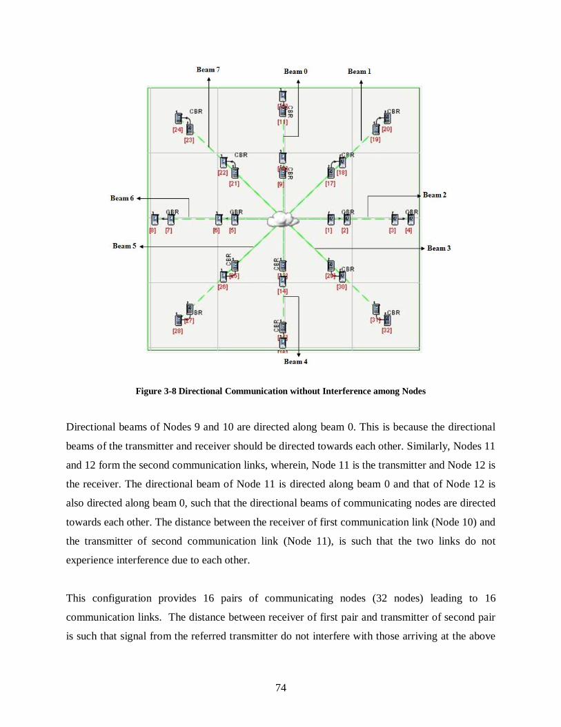
74

Figure 3-8 Directional Communication without Interference among Nodes

Directional beams of Nodes 9 and 10 are directed along beam 0. This is because the directional

beams of the transmitter and receiver should be directed towards each other. Similarly, Nodes 11

and 12 form the second communication links, wherein, Node 11 is the transmitter and Node 12 is

the receiver. The directional beam of Node 11 is directed along beam 0 and that of Node 12 is

also directed along beam 0, such that the directional beams of communicating nodes are directed

towards each other. The distance between the receiver of first communication link (Node 10) and

the transmitter of second communication link (Node 11), is such that the two links do not

experience interference due to each other.

This configuration provides 16 pairs of communicating nodes (32 nodes) leading to 16

communication links. The distance between receiver of first pair and transmitter of second pair

is such that signal from the referred transmitter do not interfere with those arriving at the above

75

mentioned receiver. An analogous explanation for the entire scenario shown in Figure 3-8 is

described through Table 3-2.

Table 3-2 Beam Orientation of Transmitting and Receiving Nodes in 32 Nodes Scenario

Beam

Number

First Communication Link Second Communication Link

Transmitting

Node

Receiving

Node

Transmitting

Node

Receiving

Node

0 9 10 11 12

1 17 18 19 20

2 1 2 3 4

3 29 30 31 32

4 13 14 15 16

5 25 26 27 28

6 5 6 7 8

7 21 22 23 24

The specifications of the scenario depicted in Figure 3-8 are given in Table 3-3. The switched

beam directional antenna model in Qualnet supports 8 directional beams, however, a node can

use only directional beam at a time. To demonstrate the possibility of directional communication

on 8 directional beams and to study the effect of interference communicating nodes, 32 nodes are

used to establish 16 communication links. These 16 communication links are distributed equally

along 8 beams of the switched beam directional antenna, details for which are provided in the

Table 3-2. In Qualnet, the default transmission range for 802.11b radio is set to 250 m (Takai,

Martin and Bagrodia 2001). The distance between the communicating nodes (transmitter and its

intended receiver) is configured as 200 m for reasons discussed in Section 3.2. These nodes are

placed on a terrain of size 3400 m2.

All the nodes communicate at 2.4 GHz and the communication between them is based on the

IEEE 802.11b standard that provides channel capacity of 11 Mbps (Forouzan 2007). The nodes

communicate directionally using switched beam directional antenna with beams oriented

according to Figure 3-7.

76

Table 3-3 Scenario Specification for Dual Polarised Communication

Parameter Value

Number of Nodes 32

Terrain Size 3400m2

Operating Frequency 2.4GHz

MAC Protocol IEEE 802.11b

Antenna Type Directional

Antenna Polarisation Vertical/Horizontal

Application CBR

Number of Packets

Transmitted

2000


Packet Interval 10ms

Data Rate 50 kbps

Transmitter Power 15dBm

Mobility None

The transmitting node generates data traffic based on the CBR traffic generation model.

According to this model, traffic source follows strict jitter and delay requirements and provides

predictable data delivery characteristics (Deng et al. 2010). The transmitter transmits 2000

packets of 512 Bytes each. The rate of data transmission is 50 kbps and interval between each

packet transmission is 10 ms. The transmission power of the transmitting nodes is set to 15 dBm

as it is the typical transmission power of nodes in Wireless LAN (USRobotics Technical Report).

The nodes in these scenarios are stationary.

Directional communication can be carried out over orthogonal polarisations (vertical and

horizontal). However, for the scenarios presented in Figure 3-8 and Figure 3-9, all the nodes

communicate using vertical polarisation. While Figure 3-8 presents the placement of nodes,

Figure 3-9 shows occurrence of communication between nodes in first and second

communication links over different directional beam orientations. The direction of arrow shows

the direction of data from transmitter to receiver, for different communication links.

77

Figure 3-9 Communication among Different Transmitter-Receiver Pairs

The beam number corresponds to the direction of orientation of the beam at the transmitter, as

explained for Figure 3-8. The scenario in Figure 3-9 demonstrates simultaneous communication

between all the pairs of transmitter and receiver nodes. 2000 packets are transmitted by the

transmitters of all the communication links to their respective receivers. The simulation results

obtained for this scenario are presented in Figure 3-10. The obtained results show that all the

packets sent by the transmitters have arrived at their respective receivers due to absence of

interference among the nodes.

In order to demonstrate the benefits of dual polarised directional communication, the node

placement in the scenario presented Figure 3-8 is changed to place the nodes within interfering

range of each other. The modified scenario is presented in Figure 3-11. As stated earlier, the

communicating nodes in scenarios presented in Figure 3-8 and Figure 3-9, use same polarisation

(vertical polarisation) for communication, leading to interference between nodes of first and

second communication links. The scenario in Figure 3-11 is then modified such that while the

nodes communicating over first communication link use vertical polarised directional antenna

78

for communication, the nodes in second communication link use horizontally polarised

directional antenna for communication.

(a) Number of packets transmitted (b) Number of packets received

Figure 3-10 Packets Sent and Received for Directional Communication of Nodes over VP when Transmitters

of First and Second Links are not in Interference Range of Each Other

The difference in performance when nodes belonging to first and second communication links

communicate over single polarisation and when they communicate over orthogonal polarisations

can be observed from the results presented in Figure 3-12 and Figure 3-13.

The scenario in Figure 3-8 is further modified to place the nodes within interference range, such

that the transmitter of second communicating link interferes with the receiver of the first

communicating link as shown in Figure 3-11. This is true for all the communication links

oriented along the direction of all the beam numbers.

79

Figure 3-11 Directional Communication where Transmitter of First Link Interferes with Transmitter of

Second Link

For this, the transmitter of the second communication link is placed in between the transmitter

and receiver of first communication link such that the two links operate along the same beam

pointing angle. With such placement of nodes, the directional beams of transmitters of first and

second communication links overlap, leading to interference. Specifications of scenario remain

same as those given in Table 3-3. Results for packets transmitted and received for this scenario

are shown in Figure 3-12.

From the results presented in Figure 3-12, it is observed that while 2000 packets (as mentioned

in Table 3-3) were transmitted, all the packets have not reached any of the receivers of the two

communication links oriented along the beam pointing angle of designated beam numbers. The

number of packets received at second receiver (receiver of second communication link) is less

than those received at the first receiver (receiver of first communication link).

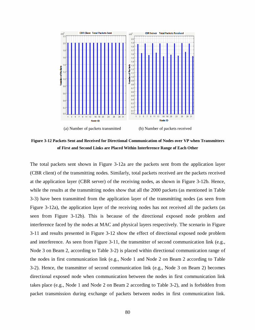
80


Figure 3-12 Packets Sent and Received for Directional Communication of Nodes over VP when Transmitters

of First and Second Links are Placed Within Interference Range of Each Other

The total packets sent shown in Figure 3-12a are the packets sent from the application layer

(CBR client) of the transmitting nodes. Similarly, total packets received are the packets received

at the application layer (CBR server) of the receiving nodes, as shown in Figure 3-12b. Hence,

while the results at the transmitting nodes show that all the 2000 packets (as mentioned in Table

3-3) have been transmitted from the application layer of the transmitting nodes (as seen from

Figure 3-12a), the application layer of the receiving nodes has not received all the packets (as

seen from Figure 3-12b). This is because of the directional exposed node problem and

interference faced by the nodes at MAC and physical layers respectively. The scenario in Figure

3-11 and results presented in Figure 3-12 show the effect of directional exposed node problem

and interference. As seen from Figure 3-11, the transmitter of second communication link (e.g.,

Node 3 on Beam 2, according to Table 3-2) is placed within directional communication range of

the nodes in first communication link (e.g., Node 1 and Node 2 on Beam 2 according to Table

3-2). Hence, the transmitter of second communication link (e.g., Node 3 on Beam 2) becomes

directional exposed node when communication between the nodes in first communication link

takes place (e.g., Node 1 and Node 2 on Beam 2 according to Table 3-2), and is forbidden from

packet transmission during exchange of packets between nodes in first communication link.

81

Hence signals transmitted by transmitter of first communication link (e.g., Node 1 on Beam 2) to

receiver of first communication link (e.g., Node 2 on Beam 2) are not corrupted due to the

transmitter of second communication link (e.g., Node 3 on Beam 2). However, when the

transmitter of second communication link (e.g., Node 3 on Beam 2) transmits to receiver of

second communication link (e.g., Node 4 on Beam 2), its directional beam is pointed towards the

receiver of second communication link (e.g., Node 4 on Beam 2). At this instance if transmitter

of first communication link (e.g., Node 1 on Beam 2) tries to access the medium it finds the

medium to be idle because it is not placed within directional communication range of the

transmitter of second communication link (e.g., Node 3 on Beam 2). This is because directional

beam of transmitter of second communication link (e.g., Node 3 on Beam 2) is formed away

from the transmitter of first communication link (e.g., Node 1 on Beam 2). Therefore, transmitter

of first communication link (e.g., Node 1 on Beam 2) does not face the directional exposed node

problem. During this instance, if transmitter of first communication link (e.g., Node 1 on Beam

2) also transmits, then the signals from the transmitter of second communication link (e.g., Node

3 on Beam 2) and transmitter of first communication link (e.g., Node 1 on Beam 2) interfere

leading to corruption of packets on both the communication links. That is why; second

communication link is more prone to interference and corruption of packets when compared to

first communication link. Therefore, the packets received by the receiver of second

communication link (e.g., Node 4 on Beam 2) are lesser than those received by the receiver of

first communication link (e.g., Node 2 on Beam 2). Hence, it can be concluded that due to

interference and problem of directional exposed node between two communication links

operating along an identical beam pointing angle, network performance has deteriorated. It must

be noted that in the scenarios presented in Figure 3-8 and Figure 3-11, all the nodes

communicate using same polarisation (VP). While this does not matter in the scenario where

nodes are placed such that they do not interfere with each other, number of packets received

drops when the nodes are placed such that they interfere with each other. The scenario shown in

Figure 3-11 is modified to prove that the use of orthogonal polarisations for communication

among the nodes located within interference range of each other helps in mitigating interference

and enhancing network performance.

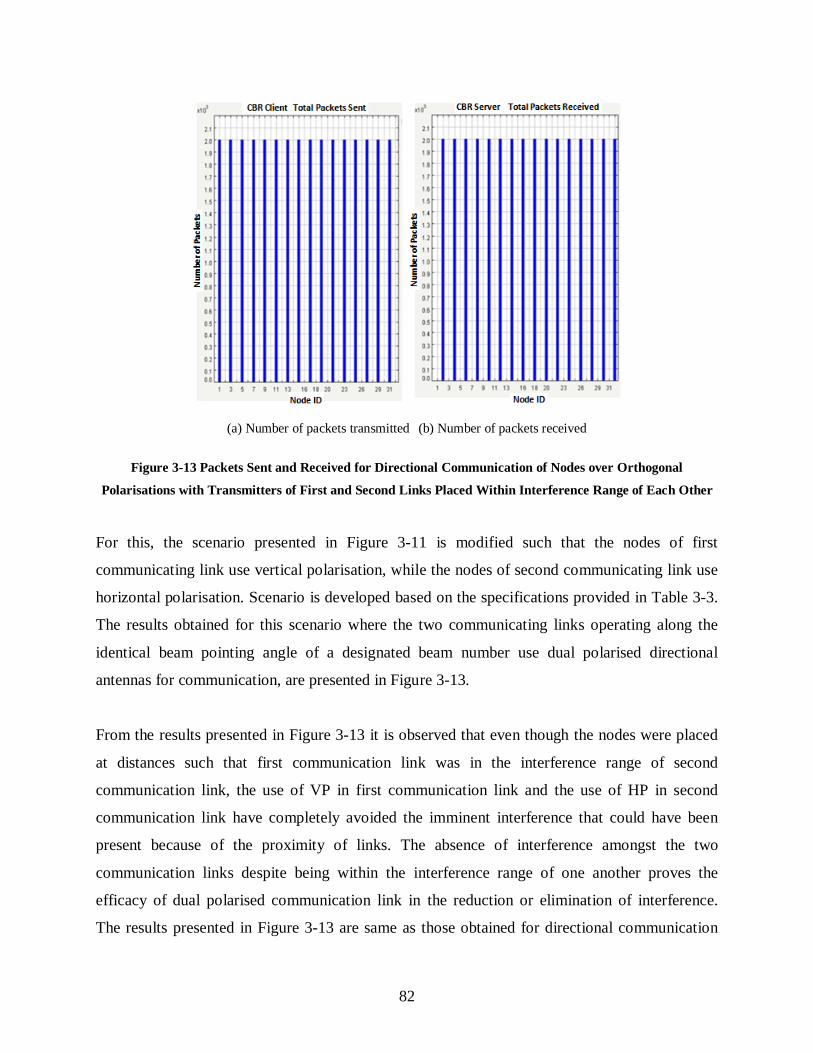
82


Figure 3-13 Packets Sent and Received for Directional Communication of Nodes over Orthogonal

Polarisations with Transmitters of First and Second Links Placed Within Interference Range of Each Other

For this, the scenario presented in Figure 3-11 is modified such that the nodes of first

communicating link use vertical polarisation, while the nodes of second communicating link use

horizontal polarisation. Scenario is developed based on the specifications provided in Table 3-3.

The results obtained for this scenario where the two communicating links operating along the

identical beam pointing angle of a designated beam number use dual polarised directional

antennas for communication, are presented in Figure 3-13.

From the results presented in Figure 3-13 it is observed that even though the nodes were placed

at distances such that first communication link was in the interference range of second

communication link, the use of VP in first communication link and the use of HP in second

communication link have completely avoided the imminent interference that could have been

present because of the proximity of links. The absence of interference amongst the two

communication links despite being within the interference range of one another proves the

efficacy of dual polarised communication link in the reduction or elimination of interference.

The results presented in Figure 3-13 are same as those obtained for directional communication

83

scenario where the nodes of the two communication links are placed such that they do not

interfere with each other. Therefore, it can be concluded that by using dual polarisation, the 16

communication links present in the scenario can operate independent of each other even if the

nodes are placed in interfering range of each other, and even if there are two communication

links along the same beam pointing angle.

3.4 Conclusion

Increased density of nodes in MANETs causes inevitable shortcoming of interference amongst

the nodes, leading to the deterioration of overall performance of the network. Therefore,

mitigation and minimisation of interference among the communicating nodes of MANET are

important tasks. Hence, it becomes essential to overcome interference among nodes in the

network. This chapter has emphasised the importance of Dual Polarised Directional Antenna

(DPDA), to mitigate interference among the nodes in the network. To study the effect of DPDA

in mitigating interference among nodes, simulation studies are carried out in Qualnet. To study

the communication among nodes operating along the beam pointing angles of 8 different

directional beams, 16 pairs of communication links are established with 32 nodes. From the

simulations, it is observed that when the nodes located within interfering range of each other

communicate using the same polarisation (vertical), they undergo interference leading to

corruption of signals at the receiver and drop of corrupted packets. However, when

communicating pair of nodes located within interference range of each other use orthogonal

polarisations, it is observed that the signals at the receiver nodes are not corrupted. From the

simulation study it is observed that when interfering communication links are configured to use

orthogonal polarisations, they virtually operate independent of each other, thus enhancing

performance of the network. This simulation demonstrates that dual polarised directional

communication can help in mitigating interference among the nodes and thus enhances network

performance.

84

CHAPTER4

4 Novel Scheme for Handling the Corruption of Broadcast Packets due to Hidden

Terminal Problem

4.1 Introduction

Routing plays a vital role in establishing communication between the nodes in a MANET.

Depending on the application and requirement, single path or multiple paths can be established

between source and destination nodes. As multipath routing provides reliability, robustness and

efficiency to network communication (Meghanathan 2010), prime goal of this thesis is to

develop an efficient multipath routing protocol for MANETs. However, the first step towards

implementing an efficient multipath routing protocol is extensive neighbour discovery, to

facilitate the establishment of unique multiple paths between the nodes. For extensive neighbour

discovery, nodes exchange broadcast packets consisting of information useful for efficient

network communication and routing. These broadcast packets are exchanged omnidirectionally

to ensure that they reach all the nodes in the vicinity, simultaneously. However, these packets

experience corruption due to a characteristic of wireless networks, known as the hidden terminal

problem or hidden node problem.This chapter presents a method to handle corruption of

broadcast packets due to hidden node problem. The hidden node problem is explained and its

effect on the nodes in the network is analysed. The importance and need of methods to handle

this problem are emphasized. The proposed method to handle corruption of broadcast packets

due to hidden node problem is explained in detail. The performance of the proposed method is

analysed through simulations. From simulations it is observed that the proposed method

overcomes the problem of corruption of broadcast packets and helps in thorough neighbour

discovery, thus developing exhaustive Neighbour Table (NT) to be used for multipath routing

and efficient network communication. The hidden node problem is discussed in Section 2.6.1.

4.2 Need for Handling Corruption of Broadcast Packets due to Hidden Node

Problem for Efficient Multipath Routing

Routing is an essential task in MANETs. With mobility of nodes, exchange of data between any

two nodes requires that the network nodes be aware of routes to carry required information from

one node to another. This makes the nodes in the network act as source, sink or router of

information. Exchange of broadcast packets is an elementary operation of any routing protocol.

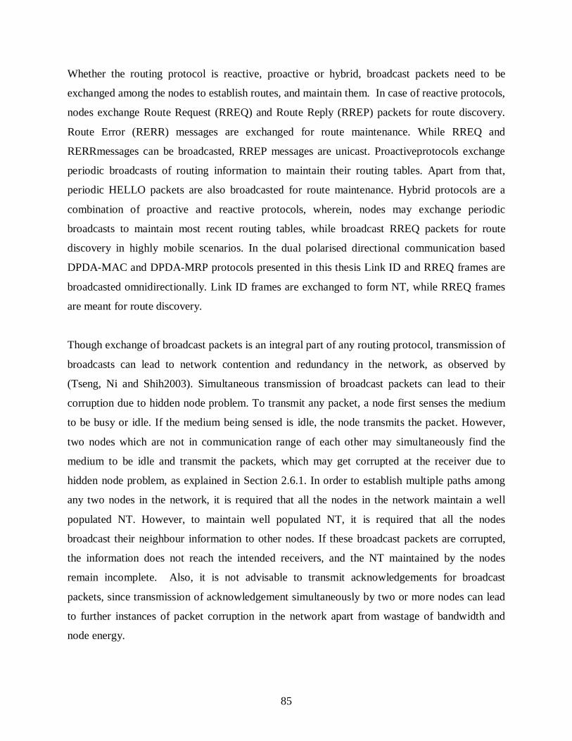
85

Whether the routing protocol is reactive, proactive or hybrid, broadcast packets need to be

exchanged among the nodes to establish routes, and maintain them. In case of reactive protocols,

nodes exchange Route Request (RREQ) and Route Reply (RREP) packets for route discovery.

Route Error (RERR) messages are exchanged for route maintenance. While RREQ and

RERRmessages can be broadcasted, RREP messages are unicast. Proactiveprotocols exchange

periodic broadcasts of routing information to maintain their routing tables. Apart from that,

periodic HELLO packets are also broadcasted for route maintenance. Hybrid protocols are a

combination of proactive and reactive protocols, wherein, nodes may exchange periodic

broadcasts to maintain most recent routing tables, while broadcast RREQ packets for route

discovery in highly mobile scenarios. In the dual polarised directional communication based

DPDA-MAC and DPDA-MRP protocols presented in this thesis Link ID and RREQ frames are

broadcasted omnidirectionally. Link ID frames are exchanged to form NT, while RREQ frames

are meant for route discovery.

Though exchange of broadcast packets is an integral part of any routing protocol, transmission of

broadcasts can lead to network contention and redundancy in the network, as observed by

(Tseng, Ni and Shih2003). Simultaneous transmission of broadcast packets can lead to their

corruption due to hidden node problem. To transmit any packet, a node first senses the medium

to be busy or idle. If the medium being sensed is idle, the node transmits the packet. However,

two nodes which are not in communication range of each other may simultaneously find the

medium to be idle and transmit the packets, which may get corrupted at the receiver due to

hidden node problem, as explained in Section 2.6.1. In order to establish multiple paths among

any two nodes in the network, it is required that all the nodes in the network maintain a well

populated NT. However, to maintain well populated NT, it is required that all the nodes

broadcast their neighbour information to other nodes. If these broadcast packets are corrupted,

the information does not reach the intended receivers, and the NT maintained by the nodes

remain incomplete. Also, it is not advisable to transmit acknowledgements for broadcast

packets, since transmission of acknowledgement simultaneously by two or more nodes can lead

to further instances of packet corruption in the network apart from wastage of bandwidth and

node energy.

86

Therefore, to implement an efficient multipath routing protocol, it is important to first handle the

corruption of broadcast packets that occurs due to hidden node problem. This helps in discovery

of maximum number of neighbours by any node to establish multiple paths to a destination. In

this chapter, a survey of methods to handle hidden node problem is provided. This is followed by

explanation of the proposed method to handle corruption of broadcast packets due to hidden

node problem accompanied with simulation results and analysis.

4.3 A Novel Scheme for Handling Corruption of Broadcast Packets due to Hidden

Node Problem

This section presents a novel method for handling the corruption of broadcast packets due to

hidden node problem. For operation of DPDA-MAC protocol each node transmits Link ID

broadcasts to inform about its presence, polarisation, idle/busy status and node location to other

nodes. These Link ID broadcasts are used for populating the NT. Well populated NT also help in

discovery of multiple routes between source and destination nodes and efficient multipath

routing. This exchange of Link ID broadcasts is also used to calculate the Received Signal

Strength Indicator (RSSI) value at the receiver, for corresponding node. The measured RSSI can

be used for optional dynamic power control. The Link ID broadcast packets are designed to

contain 2 Bytes long checksum field to indicate corruption of packets at the receiver. The

proposed method uses a Corruption Detection Pulse (CDP) for handling corruption of broadcast

packets due to hidden terminal problem. When a node receives a corrupted broadcast packet with

invalid CRC, it transmits a CDP.

The contents of the Broadcast packets areSelf Node ID (address of the node transmitting the

broadcast), Horizontal polarisation ID (status of horizontal polarisation), Vertical polarisation ID

(status of vertical polarisation), Horizontal NAV (NAV duration at horizontal polarisation),

Vertical NAV (NAV duration at vertical polarisation), X and Y Coordinates and Checksum. The

length of the broadcast frame is 208 bits.Whenever a node receives a broadcast packet with valid

CRC, it populates its NT with information about transmitter of the broadcast packet. This NT

isfurther used to establish multiple paths between source and destination nodes forproper

operation of the proposed DPDA-MAC and DPDA-MRP. An example NT is shown in Table

4-1.

87

Table 4-1 Example of Neighbour Table

Node

ID

Neighbour

Node ID

Neighbour Node

Status

Polarisation

Status

NAV

Time

(ms)

RSSI

(dBm)

Neighbour Node

Coordinates (m)

1 2 2,2 Hf 0 -79.0

0,240 2,3 Vb 30 -79.0

1 5 5,1 Hb 70 -81.0

0,0 5,10 Vb 65 -81.0

1 9 9,9 Hf 0 -77.0

240,240 9,9 Vf 0 -77.0

1 6 6,4 Hb 20 -82.0

240,0 6,6 Vf 0 -82.0

An example of a NT for Node 1 with its neighbour nodes being 2, 5, 9 and 6 is presented in

Table 4-1. The neighbour node status column presents the idle or busy status of the neighbour

nodes. Under polarisation status, ‘f’ stands for free and ‘b’ stands for busy. For example, for

neighbour Node 2, entry (2, 2) with polarisation status Hf shows that in horizontal polarisation,

Node 2 is idle, therefore, Network Allocation Value (NAV) value is zero, while (2, 3) with Vb

shows that in vertical polarisation Node 2 is busy communicating with Node 3 with a NAV of 30

ms; meaning that the ongoing communication will continue for next 30 ms.The sixth column

provides the RSSI measured at the receiver of broadcast packet. The last column provides

position coordinates of neighbour nodes. This information is used to direct the beam of

directional antenna in appropriate direction and calculate RSSI (presented in sixth column) using

Friis transmission formula, explained in Section 2.5.1 of Chapter 2. For Node 9, the entry shows

that Node 9 is idle for both vertical and horizontal polarisations. Therefore, NAV for Node 9 in

both the polarisations is 0. The sixth column provides the RSSI measured at Node 1 for Node 9.

The last column provides the position coordinates of Node 9. As the broadcast packets are

transmitted omnidirectionally in same polarisation (vertical), there are chances that these packets

get corrupted at the destination nodes due to hidden node problem. Such corrupted packets are

discarded at the receivers and are not used to populate the NT. This leads to incomplete NT,

which can further lead to incomplete RT. Performance of the proposed DPDA-MAC and

DPDA-MRP protocols degrade due to incomplete NT and RT.Therefore, it is highly important to

88

ensure development of an exhaustive NT containing most recent information about the

polarisation of neighbour node, its NAV and RSSI information. The proposed method to handle

broadcast packet corruption helps in achieving the same.

When a node receives a broadcast packet with corrupted CRC, it discards the received data and

without waiting for a backoff time, it immediately transmits a CDP of 8µs duration. The duration

of CDP is configured as 8µs because it is observed in (Shih et al., 2009) and (Yang and Vaidya

2002) that a tone/pulse with a minimum duration of 5µs can be easily detected by the nodes in

the wireless network. Multiple nodes that detect a corrupted broadcast packet can transmit CDP

simultaneously, which may overlap. The transmitter of the broadcast packets senses the medium

for one broadcast packet transmission time. This is the time it takes for the broadcast packet to

travel in the medium. It can vary with varying channel bit rate.As the length of broadcast frame

is 208 bits, time taken for the broadcast packet to travel the medium with channel capacity of 2

Mbps is 104 µs. For the medium with channel capacity of 11 Mbps the time taken for the

broadcast packet to travel the medium is 19 µs and it reduces to 4µs when capacity of the

channel is increased to 54 Mbps. Whenever a node detects a 5µs long pulse, it considers that

corruption of broadcast packet has taken place. When a transmitter detects the presence of CDP

in the medium immediately after transmission of broadcast packet, it retransmits the broadcast

packet.However, there needs to be a limit on the number of rebroadcasts. As demonstrated in

(Tseng et al. 2002), rebroadcasting 3 to 4 times provide a good tradeoff between connectivity

and congestion. It is observed that number of broadcasts limited to 3 to 4, provides good

connectivity and reachability, while not leading to network congestion.

The proposed method for handling corruption of broadcast packets due to hidden terminal

problem is explained through the flowchart in Figure 4-1 and Figure 4-2. A node intending to

transmit first senses the medium to be idle or busy. When the medium becomes idle, the node

transmits the broadcast packet. After transmission of broadcast packet the transmitter switches to

receive mode.

89

Figure 4-1 Flowchart to Overcome Hidden Node Problem

Start

Transmitter senses the medium

Is medium busy?

No

DIFS + Random delay Yes

Carrier idle ?

Yes

Transmit Broadcast

Transmitter switches to receive mode

Neighbour nodes receive broadcast

A B

No

90

Figure 4-2 Flowchart to Overcome Hidden Node Problem (Continued)

If the neighbour nodes of the transmitter receive the broadcast packet without corruption, then

the transmission of the broadcast packet is considered to be successful. However, if the received

broadcast packet is corrupted, the receiving node switches to transmitting mode and transmits

CPD. On receiving CDP, the transmitter of broadcast packet tries to retransmit the broadcast

A B

Packet corrupted?

Success

Receiver sends CDP without backoff

Transmitter receives CDP and increments retransmission

counter

Retransmission limit reached? Abort

Increment backoff delay

No Yes

Yes

No

91

packet. For this, it first increments the retransmission counter and checks if retransmission limit

has reached. If the retransmission limit has reached, the transmitter aborts the transmission.

Otherwise, it increments the backoff delay and again waits for the medium to be idle before

transmission of the broadcast packet.

The proposed method for handling the corruption of broadcast packets can be analysed for four

different cases. All these cases assume static nodes and symmetric links. The presence of two-

way arrows between nodes indicates the presence of symmetric communication link between the

nodes, while absence of the arrows represents absence of communication link.

Case 1

In Figure 4-3, bidirectional link exists between Nodes A-B, C-D and C-E implying that the nodes

are within communication range of each other. Nodes D and E are in communication range of

Node C.

Figure 4-3Case 1 for Broadcast Packet Corruption due to Hidden Node Problem

If Nodes D and E transmit a broadcast packet simultaneously, or their transmission overlaps in

time, then there is a possibility of corruption of these packets at C, due to hidden node problem.

On detecting packet corruption, Node C immediately transmits CDP, without any backoff delay.

On detecting CDP immediately after broadcast transmission, Nodes D and E try to retransmit the

broadcast packet with increased backoff limit.

The sequence of events is displayed in the Figure 4-4along with their timing information. As

seen from the timing diagram, Node D transmits the broadcast packet at 34.632 ms, and Node E

transmits the broadcast packet at 34.693 ms. As their transmissions overlap in time, corruption of

broadcast packets is detected at Node C, at 34.737 ms. On detecting a corrupted broadcast frame,

92

Node C transmits CDP without backoff. On detecting CDP in the medium, Nodes D and E

increase their backoff period and retransmit the broadcast packet. Details about increase of

backoff period are presented in Section 4.4.

Figure 4-4Timing Diagram for Case 1

As mentioned earlier, after transmission of broadcast packet, transmitter waits for another

broadcast frame transmission time. If the node receives CDP within this time, it retransmits the

broadcast packet, otherwise it ignores the CDP. With every retry, the transmitting node increases

the backoff period by 10µs. In the given scenario, if Nodes A and C transmit simultaneous

broadcasts, there will be no packet corruption at any of the nodes.

Case 2

Case 2 is presented in Figure 4-5, where symmetric communication links exist between Nodes E-

A, B-A, B-C, and C-D. There is no communication link between Nodes A and C, Nodes E and

B, Nodes D and B. The scenario presented in this case is different from that presented in Case 1

since the aim to include this scenario is to show how the nodes which have received the

broadcast packet correctly in first transmission itself, react to retransmission of broadcast.


93

In this case, if Nodes A and C transmit a broadcast packet simultaneously, or their transmission

overlaps in time, then Node B may detect corrupted broadcast packet, while Nodes E and D may

receive the broadcasts without corruption. Immediately after detecting a corrupted packet, Node

B transmits a CDP. Since Nodes E and D are not within the communication range of Node B,

they do not get affected by the CDP transmitted by Node B.

While Nodes A and C try to retransmit the broadcast packet with increased backoff, Nodes E and

D use correctly received broadcast packet to populate their NT. Retransmitted broadcast packets

are again received by Nodes E and D, used for updating the NT information again.


As seen from the timing diagram presented in Figure 4-6, Nodes D and E receive uncorrupted

broadcast packets twice from Nodes C and A respectively. Every time a broadcast packet is

received, it is used to update the NT.

Case 3

In Case 1 and Case 2 presented in Figure 4-3 and Figure 4-5 respectively, only one node detects

corruption of broadcast packets and transmits CDP. Case 3 for broadcast packet corruption due

to hidden node problem where multiple nodes detect corruption of broadcast packets and

transmit CPD is presented in Figure 4-7. Here, bidirectional links exist between Nodes F-A, A-E,

A-B, A-D, E-B, B-D, E-C, B-C, D-C and C-G. Nodes E, B and D are in the communication

94

range of each other and that of Nodes A and C. Nodes F and G are only within the

communication range of Nodes A and C, respectively. Nodes A and C are not in range of each

other. When Nodes A and C transmit a broadcast packet simultaneously, corruption of broadcast

packet can be experienced at Nodes E, B and D, due to hidden node problem.

However, if Nodes G and F transmit the broadcast packet simultaneously, there will be no packet

corruption, and Nodes A and C can populate their NT accordingly. After identifying the

corrupted packet, Nodes E, B and D transmit CDP of 8µs duration, without any backoff. The

CDPs transmitted by Nodes E, B and D may overlap, due to processing and propagation delays.

Whenever a node listens to CDP of minimum 5µs duration immediately after broadcast

transmission, it retransmits the broadcast packet with increased backoff.


Therefore, after sensing the CDP transmitted by Nodes E, B and D, Nodes A and C try to

retransmit the broadcast packets with increased backoff time. The sequence of events with timing

information for Case 3 is presented in Figure 4-8.

From the timing diagram it is observed that when Nodes A and C broadcast simultaneously,

Nodes E, B and D detect corrupted broadcast packets, while Nodes F and G receive their

respective broadcast packets correctly to update their NT. On detecting packet corruption, Nodes

E, B and D transmit CDP which may overlap.

95


On detecting CDP of minimum duration of 8µs, Nodes A and C retransmit broadcast packet with

increased backoff. Nodes F and G receive the retransmitted broadcast packets again and use

them to update NT.

Case 4

In Case 1, 2 and 3, it is studied how corruption of broadcast packets is detected and broadcast

packets are retransmitted to form and maintain most recent NT. It is observed that transmission

of CDP helps in neighbour discovery to maintain well populated NT. However, transmission of

CDP without backoff can cause corruption of ongoing reception of broadcast packets by other

nodes. This leads to more CDP transmissions by receivers of corrupted broadcast packets. Case 4

discusses this possibility in detail through the scenario presented in Figure 4-9.

In the scenario illustrated in Figure 4-9, bidirectional links exist between Nodes A-E, A-B, E-B,

B-C, B-D and C-D. Nodes A and E are within the communication range of each other and that of

Node B. Similarly, Nodes C and D are also within the communication range of each other and

that of Node B. When Nodes A and C transmit a broadcast packet, it may corrupt at Node B. On

receiving a corrupted packet, Node B transmits CDP. In this scenario, there are two possibilities

for Nodes E and D.

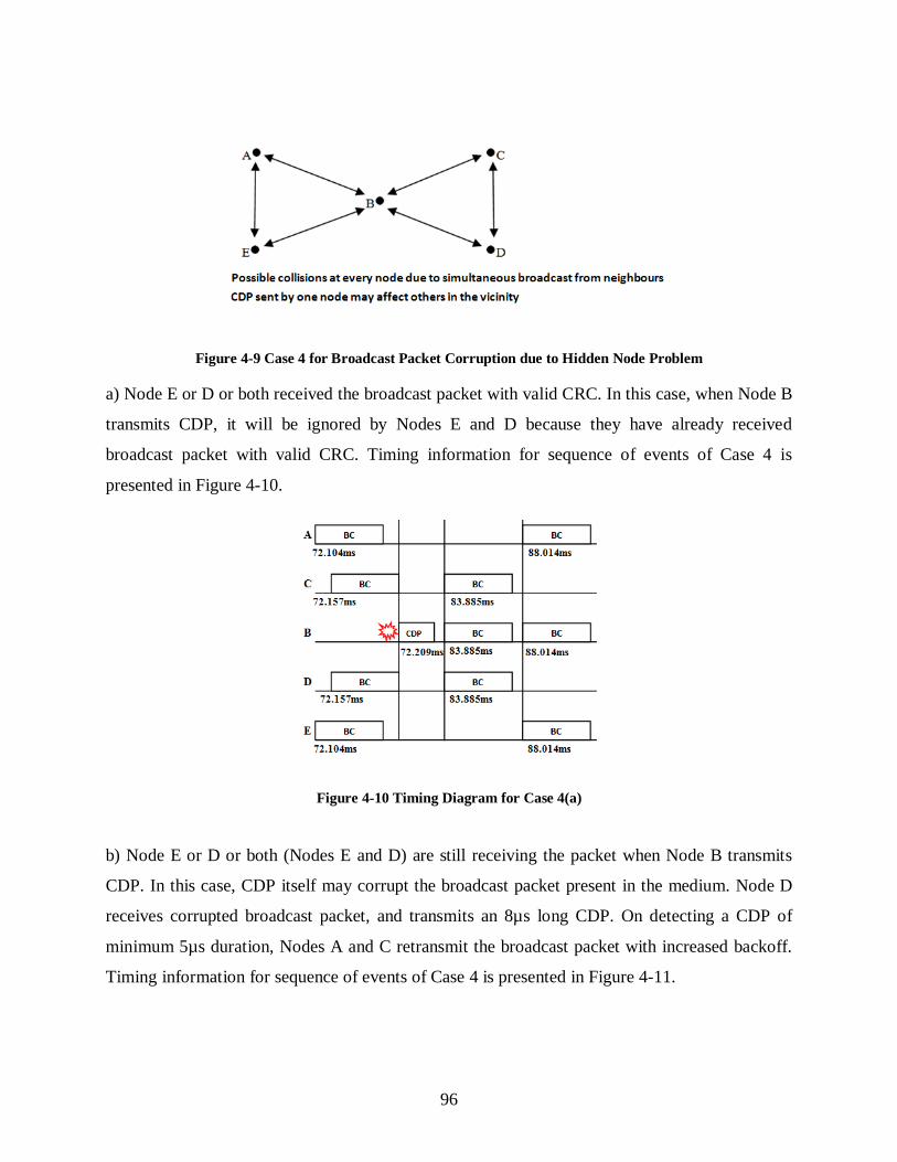
96

Figure 4-9 Case 4 for Broadcast Packet Corruption due to Hidden Node Problem

a) Node E or D or both received the broadcast packet with valid CRC. In this case, when Node B

transmits CDP, it will be ignored by Nodes E and D because they have already received

broadcast packet with valid CRC. Timing information for sequence of events of Case 4 is

presented in Figure 4-10.

Figure 4-10 Timing Diagram for Case 4(a)

b) Node E or D or both (Nodes E and D) are still receiving the packet when Node B transmits

CDP. In this case, CDP itself may corrupt the broadcast packet present in the medium. Node D

receives corrupted broadcast packet, and transmits an 8µs long CDP. On detecting a CDP of

minimum 5µs duration, Nodes A and C retransmit the broadcast packet with increased backoff.

Timing information for sequence of events of Case 4 is presented in Figure 4-11.

97

Figure 4-11 Timing Diagram for Case 4(b)

It must be noted that in this case, the CDP affects the network communication negatively. This

can be perceived as the drawback of the proposed technique.

4.4 Simulation and Analysis of Proposed Method for Handling Corruption of

Broadcast Packets for Discovery of Neighbour Nodes

The proposed scheme to handle corruption of broadcast packets while neighbour discovery is

simulated using a simulator developed in C++ (details of the developed simulator are presented

in Appendix 1), and performance of the simulated scheme is tested. All the nodes in a MANET

transmit periodic broadcast packets to notify about their presence in the network to their

neighbours. As stated earlier, the principal aim of developing this scheme is to ensure efficient

neighbour node discovery for operation of the dual polarised directional antenna based proposed

DPDA-MAC and DPDA-MRP protocols. To establish dual polarised directional antenna based

communication, nodes need to broadcast information about their free and busy polarisation,

NAV duration for busy polarisation, coordinates of node for directional communication, apart

from self node ID and checksum. Corruption of broadcast packets leads to incomplete NT.

Nodes that could not be discovered due to corruption of broadcast packets transmitted by them

are termed as ‘missed nodes’. If a node fails to discover all its neighbours as a result of

corruption of broadcast packets due to hidden node problem, then an efficient multipath routing

protocol cannot be developed.

98

Before transmitting the broadcast packet over the wireless medium, a node first senses the

medium to be idle. If the medium is not idle, node waits for the medium to become idle. When

the medium becomes idle, node waits for 50µs plus a random interval of time. Contention period

is decided based on random number generated between minimum and maximum number of time

slots for contention. Minimum value of CW time slots (CWmin) is 31, while maximum value

(CWmax) is 1023. The duration of each time slot of CW is 20µs (IEEE 802 LAN/MAN Standards

Committee 1999). A random value is generated between 31 and 1023 to decide the number of

time slots for Contention Window (CW). After every failed attempt, the transmitter increases the

backoff by 10 µs. Therefore, for the very first attempt, waiting period for a node after idle

channel sensing is given by Equation 4.1.

50𝜇𝜇𝑠𝑠 + 20𝜇𝜇𝑠𝑠 × (𝑟𝑟𝑑𝑑𝐼𝐼𝑑𝑑(31,1023)) ...4.1

For every retry, the transmitter increases the backoff period by 10µs. Therefore, ‘n’ being the

number of reattempts, the waiting period for every backoff is given by Equation 4.2.

50𝜇𝜇𝑠𝑠 + (𝐼𝐼 × 10𝜇𝜇𝑠𝑠) + 20𝜇𝜇𝑠𝑠 × (𝑟𝑟𝑑𝑑𝐼𝐼𝑑𝑑(31,1023)) ...4.2

where, ‘n’ varies from 1 to 4.

To test and verify the proposed scheme, simulations are carried out based on the scenario

specifications are presented in Table 4-2. These simulations are carried out in a simulator

implemented in C++. The details of the developed simulator are presented in Appendix 1. The

scenario aims to study the effect of increase in density of nodes on the instances of corruption of

Link ID broadcasts due to hidden terminal problem and test the performance of the proposed

scheme. To achieve this, the terrain size is kept constant to 1000 x 1000 m2, while increasing the

number of nodes in the network. The nodes in the network are placed in grid topology. Grid

topology is used for this study because it includes all the cases covered in Section 4.3. Keeping

the terrain size same (1000 x 1000 m2), grid size is represented as (n x n) where ‘n’ varies from 6

to 25 in steps of one. Therefore, the minimum number of nodes in the network is 36 and

maximum number of nodes is 625.

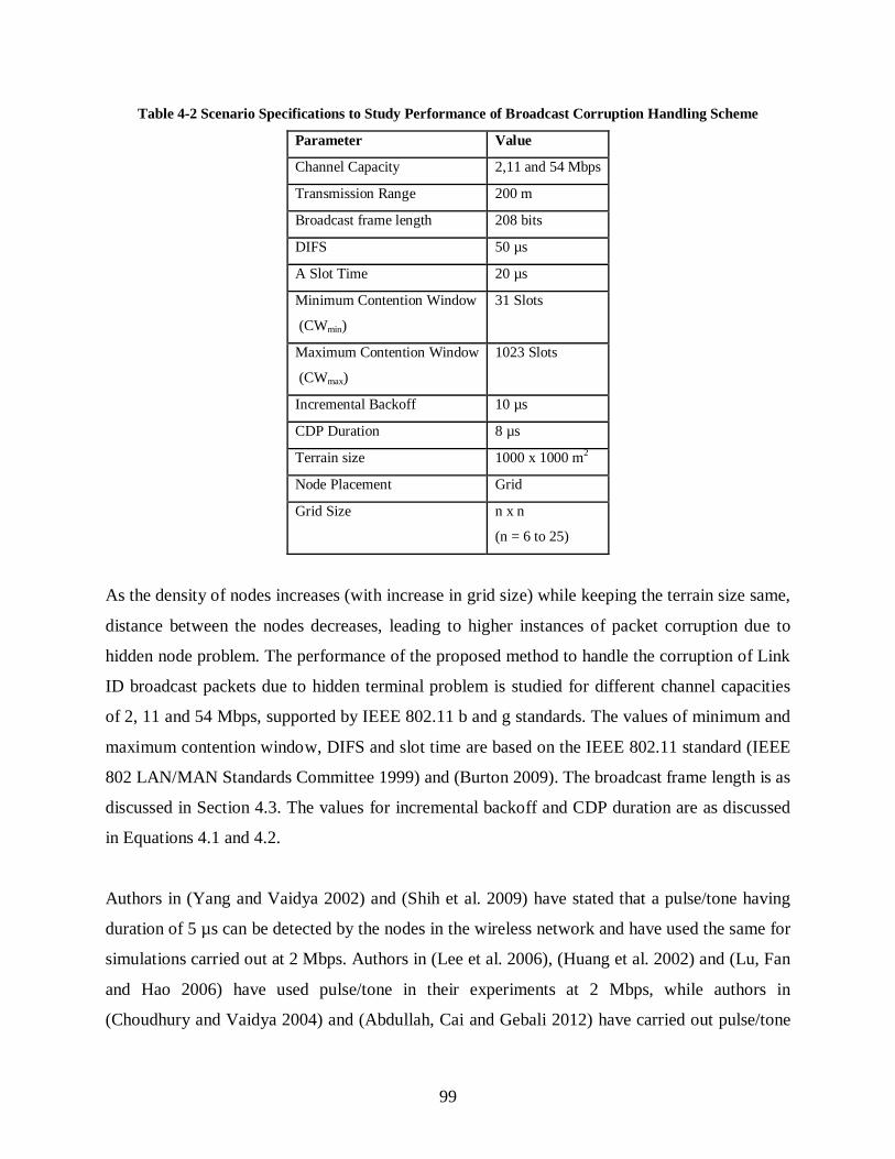
99

Table 4-2 Scenario Specifications to Study Performance of Broadcast Corruption Handling Scheme

Parameter Value

Channel Capacity 2,11 and 54 Mbps

Transmission Range 200 m

Broadcast frame length 208 bits

DIFS 50 µs

A Slot Time 20 µs

Minimum Contention Window

(CWmin)

31 Slots

Maximum Contention Window

(CWmax)

1023 Slots

Incremental Backoff 10 µs

CDP Duration 8 µs

Terrain size 1000 x 1000 m2

Node Placement Grid

Grid Size n x n

(n = 6 to 25)

As the density of nodes increases (with increase in grid size) while keeping the terrain size same,

distance between the nodes decreases, leading to higher instances of packet corruption due to

hidden node problem. The performance of the proposed method to handle the corruption of Link

ID broadcast packets due to hidden terminal problem is studied for different channel capacities

of 2, 11 and 54 Mbps, supported by IEEE 802.11 b and g standards. The values of minimum and

maximum contention window, DIFS and slot time are based on the IEEE 802.11 standard (IEEE

802 LAN/MAN Standards Committee 1999) and (Burton 2009). The broadcast frame length is as

discussed in Section 4.3. The values for incremental backoff and CDP duration are as discussed

in Equations 4.1 and 4.2.

Authors in (Yang and Vaidya 2002) and (Shih et al. 2009) have stated that a pulse/tone having

duration of 5 µs can be detected by the nodes in the wireless network and have used the same for

simulations carried out at 2 Mbps. Authors in (Lee et al. 2006), (Huang et al. 2002) and (Lu, Fan

and Hao 2006) have used pulse/tone in their experiments at 2 Mbps, while authors in

(Choudhury and Vaidya 2004) and (Abdullah, Cai and Gebali 2012) have carried out pulse/tone

100

based simulations at 11 Mbps. However, minimum required duration for pulse/tone is not

mentioned in these papers. Authors in (Haas and Deng 2002) have stated that the delay in

detection of pulse/tone is a characteristic of communication hardware. Therefore, based on the

information obtained from available literature, in the simulations carried out in this thesis,

pulse/tone with minimum duration of 5 µs is taken as benchmark for all data rates (2, 11 and 54

Mbps), with belief that when a pulse/tone with duration of 5 µs can be detected at 2 Mbps, it will

be long enough to be easily detected by nodes in wireless network at 11 and 54 Mbps as well.

However, as pointed in (Haas and Deng 2002), the delay in detection of pulse/tone is a

characteristic of communication hardware. Therefore, in practical systems or simulations where

these characteristics of communication hardware are known, the pulse duration can be varied

accordingly.

MANETs are highly dynamic temporary networks, which are established between mobile nodes

that may join the network briefly and leave after carrying out required communication, or due to

node mobility. Some of the applications of MANETs comprise of establishing Infrastructureless

network during emergency or rescue operations, temporary networks to exchange data in

meetings or conferences and data exchange between vehicles (VANETs) (Macker and Corson

2004). Therefore, most likely, MANETs will be networks of mixed type comprising of devices

with network interface cards (NICs) that could support 2 Mbps, 11 Mbps and 54 Mbps, as in a

temporary and dynamic network like MANET, it is difficult to ensure or control participation of

devices that support only 2 Mbps or only 11 Mbps or only 54 Mbps. In such case, a CDP

transmitted by a device with NIC supporting 54 Mbps should also be sensed by the device

supporting 2 Mbps / 11 Mbps, and vice-versa. Hence, in the simulations carried out in this thesis

the duration of CDP is configured to be same (8 µs) for all values of channel capacity (2 Mbps,

11 Mbps and 54 Mbps).The duration of CDP is kept as 8 µs for easy computation and

implementation. In simulation, the CDP is implemented as a packet with its size varying with

data rate, such that the packet duration of 8 µs can be accounted for. Therefore, at 2 Mbps the

CDP is 2 Bytes long, at 11 Mbps the CDP is 11 Bytes long and at 54 Mbps it is 54 Bytes long.

Computation of CDP duration at 2 Mbps is shown through Equation 4.3. Let ‘𝑥𝑥’ be the size of

the pulse to achieve duration of 8 µs. Then, at 2 Mbps, the size of the pulse can be computed as

101

2 ×106

1= 𝑥𝑥

8×10−6 ∴ 𝑥𝑥 = (2 × 8) Bits or 2 Bytes ...4.3

Similarly, the size of pulse at 11 Mbps can be computed as 11 Bytes and that at 54 Mbps can be

computed as 54 Bytes.

Because of mixed specification of devices participating in practical MANETs, long slot time of

20 µs and corresponding DIFS, SIFS times are used (Burton 2009). Therefore, for simulation of

MANETs carried out in this work slot time of 20 µs, SIFS of 10 µs, DIFS of 50 µs and

contention window (31, 1023) is used for all values of channel capacity (2 Mbps, 11 Mbps and

54 Mbps) (Burton 2009).

As specified in (Burton 2009), Short slot time of 9 µs can be configured and used only if it is

ensured that all the participating nodes support 802.11g standard (which is difficult to ensure in a

dynamic network like MANET). Such networks where all participating nodes would support

802.11g standard can use shorter slot times and interframe spaces thus achieving enhanced

network throughput when compared to mixed network (comprising of devices supporting

802.11, 802.11b and 802.11g standards).

The performance of the proposed scheme is compared with that of IEEE 802.11 DCF, wherein

there is no concept of transmission of CDP by the receiving node on detecting a corrupted

packet. The results obtained with single transmission attempt, (Attempt 1) do not include the

concept of CDP transmission. In case of corruption of broadcast packets transmitted in Attempt

1, the proposed method of broadcast corruption handling takes place (transmission of CDP) and

broadcast packets are retransmitted with increased backoff. To limit the number of rebroadcasts,

the maximum retry limit is set to 4. Therefore, every node can retransmit the broadcast packets 4

times at the most. These attempts are represented as Attempts 2, 3, 4 and 5. The performance of

the proposed scheme is tested in terms of the number of neighbours discovered, as that is the

primary goal of the proposed scheme. Based on the scenario specifications given in Table 4-2,

the results are plotted as Number of Neighbour Nodes Missed vs. Number of Nodes present in

the network, for different transmission attempts and varying channel capacities. These results are

presented based on the NT entries of nodes with varying node densities. As the nodes are

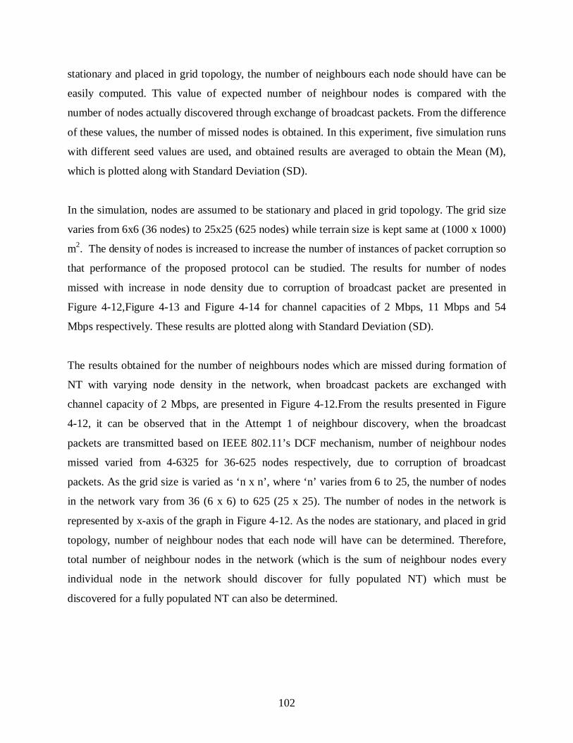
102

stationary and placed in grid topology, the number of neighbours each node should have can be

easily computed. This value of expected number of neighbour nodes is compared with the

number of nodes actually discovered through exchange of broadcast packets. From the difference

of these values, the number of missed nodes is obtained. In this experiment, five simulation runs

with different seed values are used, and obtained results are averaged to obtain the Mean (M),

which is plotted along with Standard Deviation (SD).

In the simulation, nodes are assumed to be stationary and placed in grid topology. The grid size

varies from 6x6 (36 nodes) to 25x25 (625 nodes) while terrain size is kept same at (1000 x 1000)

m2. The density of nodes is increased to increase the number of instances of packet corruption so

that performance of the proposed protocol can be studied. The results for number of nodes

missed with increase in node density due to corruption of broadcast packet are presented in

Figure 4-12,Figure 4-13 and Figure 4-14 for channel capacities of 2 Mbps, 11 Mbps and 54

Mbps respectively. These results are plotted along with Standard Deviation (SD).

The results obtained for the number of neighbours nodes which are missed during formation of

NT with varying node density in the network, when broadcast packets are exchanged with

channel capacity of 2 Mbps, are presented in Figure 4-12.From the results presented in Figure

4-12, it can be observed that in the Attempt 1 of neighbour discovery, when the broadcast

packets are transmitted based on IEEE 802.11’s DCF mechanism, number of neighbour nodes

missed varied from 4-6325 for 36-625 nodes respectively, due to corruption of broadcast

packets. As the grid size is varied as ‘n x n’, where ‘n’ varies from 6 to 25, the number of nodes

in the network vary from 36 (6 x 6) to 625 (25 x 25). The number of nodes in the network is

represented by x-axis of the graph in Figure 4-12. As the nodes are stationary, and placed in grid

topology, number of neighbour nodes that each node will have can be determined. Therefore,

total number of neighbour nodes in the network (which is the sum of neighbour nodes every

individual node in the network should discover for fully populated NT) which must be

discovered for a fully populated NT can also be determined.

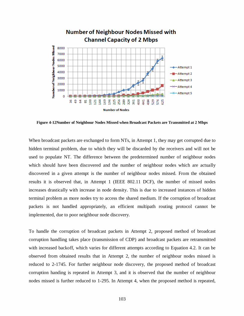
103

Figure 4-12Number of Neighbour Nodes Missed when Broadcast Packets are Transmitted at 2 Mbps

When broadcast packets are exchanged to form NTs, in Attempt 1, they may get corrupted due to

hidden terminal problem, due to which they will be discarded by the receivers and will not be

used to populate NT. The difference between the predetermined number of neighbour nodes

which should have been discovered and the number of neighbour nodes which are actually

discovered in a given attempt is the number of neighbour nodes missed. From the obtained

results it is observed that, in Attempt 1 (IEEE 802.11 DCF), the number of missed nodes

increases drastically with increase in node density. This is due to increased instances of hidden

terminal problem as more nodes try to access the shared medium. If the corruption of broadcast

packets is not handled appropriately, an efficient multipath routing protocol cannot be

implemented, due to poor neighbour node discovery.

To handle the corruption of broadcast packets in Attempt 2, proposed method of broadcast

corruption handling takes place (transmission of CDP) and broadcast packets are retransmitted

with increased backoff, which varies for different attempts according to Equation 4.2. It can be

observed from obtained results that in Attempt 2, the number of neighbour nodes missed is

reduced to 2-1745. For further neighbour node discovery, the proposed method of broadcast

corruption handing is repeated in Attempt 3, and it is observed that the number of neighbour

nodes missed is further reduced to 1-295. In Attempt 4, when the proposed method is repeated,

104

this number falls to 1-16, and by Attempt 5, all the nodes are able to discover all their neighbour

nodes. In all the attempts, maximum undiscovered neighbour nodes occur with highest node

density. This is because high node density leads to more instances of hidden terminal problem.

Therefore, in the simulated scenario, when broadcast packets are transmitted with channel

capacity of 2 Mbps, it takes 46 ms-259 ms for all nodes to discover all their neighbour nodes,

and it also implies the end of Attempt 5. When the proposed method of broadcast corruption

avoidance by transmission of CDP is used (in Attempts 2, 3, 4 and 5), it is observed that the

number of nodes missed reduces drastically. Therefore, using the proposed method, fully

populated NTs can be attained for efficient multipath routing.

Figure 4-13 Number of Neighbour Nodes Missed when Broadcast Packets are Transmitted at 11Mbps

The simulation is repeated with transmission of broadcast packets for channel capacities of 11

Mbps and 54 Mbps, and results are presented in Figure 4-13 and Figure 4-14 respectively. As

observed from the results presented in Figure 4-13, at 11 Mbps the number of neighbour nodes

missed in Attempt 1 vary from 2-1362 and it drops to 1-79 in Attempt 2. In Attempt 3, almost all

neighbour nodes are discovered. During Attempt 4 fully populated NTs are attained for efficient

multipath routing. At 11 Mbps it takes 42 ms-177 ms for all the nodes to discover all their

neighbour nodes by the end of Attempt 5.

105

Figure 4-14 Number of Neighbour Nodes Missed when Broadcast Packets are Transmitted at 54Mbps

Similarly, from results presented in Figure 4-14 it is observed that when broadcast packets are

transmitted with channel capacity of 54 Mbps, the number of neighbour nodes missed in Attempt

1 vary from 1-189 while after Attempt 2 all the nodes successfully discover all their neighbour

nodes. At 54 Mbps it takes 40ms-143ms for all the nodes to discover all their neighbour nodes

by the end of fifth attempt. It is worth noticing that number of neighbour nodes missed with

channel capacity of 2 Mbps is highest and that with channel capacity 54 Mbps is least. This is

because when channel capacity is less, the broadcast packet is present in medium for long

because it is transmitted slower than when channel capacity is high, thus increasing the chances

of packet corruption. Higher instances of corruption of broadcast packets over links with lower

channel capacity increases the number of neighbour nodes missed during discovery of neighbour

nodes in the network. From the results presented in Figure 4-12, Figure 4-13 and Figure 4-14 it is

observed that many neighbour nodes remain undiscovered in first attempt of node discovery.

Hence, next attempt with the proposed method for handling corruption of broadcast packets is

carried out. This method involves transmission of CDP and retransmission of broadcast packets

that underwent corruption.

The values of standard deviation (SD) with respect to mean (M) are presented in Table 4-3, for

different values of channel capacity and node density (number of nodes). To keep the length of

the table concise these values are presented only for Attempt 1 and Attempt 5, for selected values

106

of node density. However, standard deviation is indicated for all values of node density for

results presented in Figure 4-12, Figure 4-13 and Figure 4-14.

Table 4-3 Standard Deviation with respect to Mean for Number of Nodes Missed during Node Discovery

Number

of

Nodes

2 Mbps 11 Mbps 54 Mbps

Attempt 1 Attempt 5 Attempt 1 Attempt 5 Attempt 1 Attempt 5

M SD M SD M SD M SD M SD M SD

36 4 3.9 0 0 2 4 0 0 1 2 0 0

100 33 7.8 0 0 5 9.1 0 0 1 2 0 0

196 311 29 1 1 36 26.8 0 0 14 7 0 0

324 1102 151 3 5.8 254 101 0 0 94 56.2 0 0

484 3766 319 6 11 700 243 0 0 132 72.2 0 0

625 6325 357 13 4.4 1362 266 1 0 189 71 0 0

From Figure 4-12, Figure 4-13 and Figure 4-14, and Table 4-3it is observed that standard

deviation is more when density of nodes is high. This is because at higher node density, more

nodes try to access the shared medium leading to more instances of packet corruption and

random backoff delays. Also, the standard deviation is high in first attempt and reduces with

consecutive attempts. This is because in consecutive attempts only the nodes whose

transmissions got corrupted in previous attempts participate in retransmission. This trend is

observed over all the values of channel capacities (2 Mbps, 11 Mbps and 54 Mbps).

The total time taken to discover all the possible neighbour nodes for different grid sizes is

presented in Figure 4-15to Figure 4-19for 1 to 5 attempts respectively, along with standard

deviation. The total time taken for discovery of neighbour nodes for first attempt, with varying

channel capacity is presented in Figure 4-15. The first attempt does not include transmission of

CDP on detection of a corrupted packet at the receiver, while all other attempts incorporate the

proposed method transmission of CDP on detection of corrupted packet and retransmission of

broadcast packets which underwent corruption.

107

Figure 4-15Total Time Taken for Neighbour Node Discovery for 1 Attempt

For a network of nodes placed in grid topology with grid size ‘n x n’, where ‘n’ is varied from 6

to 25, total time taken for neighbour node discovery when broadcast packets are transmitted with

varying channel capacity is measured. From the obtained results shown in Figure 4-15, it is

observed that as the node density increases, total time taken for node discovery increases over all

the channel bit rates. This is expected because with increase in grid size and node density,

contention for shared medium and number of neighbour nodes to be discovered increases. From

the results presented in Figure 4-15, it is seen that the total time taken for neighbour node

discovery with channel capacity of 2 Mbps varies from 46ms-143ms as node density increases

from 36-625 due to increase in grid size, as explained earlier. Similarly, total time taken for

neighbour node discovery with channel capacity of 11Mbps varies from 42ms-136ms. With

channel capacity of 54Mbps the total time taken for neighbour discovery varies from 40ms-

134ms.The total time taken when discovery of neighbour nodes is carried out for two attempts is

presented in Figure 4-16. When neighbour node discovery is carried out over channel capacity of

2 Mbps, total time taken for node discovery increases with increase in number of nodes, and

varies from 47 ms for 36 nodes to 213 ms for 625 nodes. For neighbour node discovery carried

out over channel capacity of 11 Mbps, the time varies from 43 ms for 36 nodes to 173 ms for 625

nodes. For channel capacity of 54 Mbps, the total time taken for neighbour node discovery varies

from 40 ms for 36 nodes to 143 ms for 625 nodes.

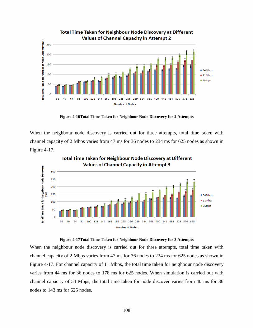
108

Figure 4-16Total Time Taken for Neighbour Node Discovery for 2 Attempts

When the neighbour node discovery is carried out for three attempts, total time taken with

channel capacity of 2 Mbps varies from 47 ms for 36 nodes to 234 ms for 625 nodes as shown in

Figure 4-17.


When the neighbour node discovery is carried out for three attempts, total time taken with

channel capacity of 2 Mbps varies from 47 ms for 36 nodes to 234 ms for 625 nodes as shown in

Figure 4-17. For channel capacity of 11 Mbps, the total time taken for neighbour node discovery

varies from 44 ms for 36 nodes to 178 ms for 625 nodes. When simulation is carried out with

channel capacity of 54 Mbps, the total time taken for node discover varies from 40 ms for 36

nodes to 143 ms for 625 nodes.

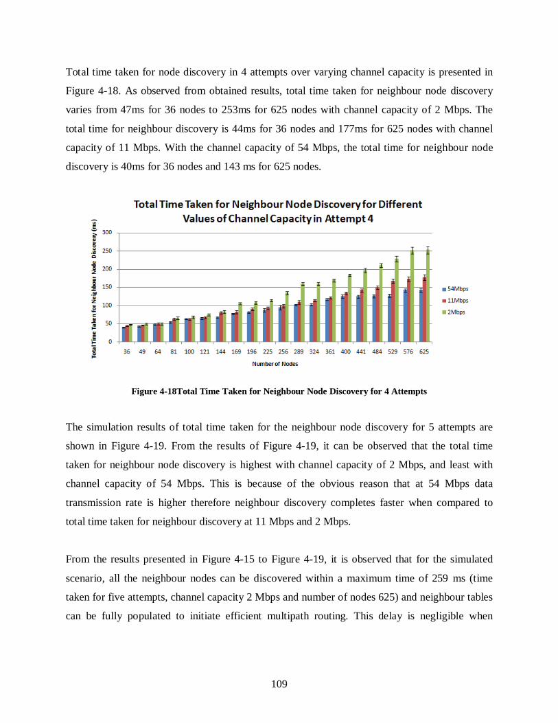
109

Total time taken for node discovery in 4 attempts over varying channel capacity is presented in

Figure 4-18. As observed from obtained results, total time taken for neighbour node discovery

varies from 47ms for 36 nodes to 253ms for 625 nodes with channel capacity of 2 Mbps. The

total time for neighbour discovery is 44ms for 36 nodes and 177ms for 625 nodes with channel

capacity of 11 Mbps. With the channel capacity of 54 Mbps, the total time for neighbour node

discovery is 40ms for 36 nodes and 143 ms for 625 nodes.


The simulation results of total time taken for the neighbour node discovery for 5 attempts are

shown in Figure 4-19. From the results of Figure 4-19, it can be observed that the total time

taken for neighbour node discovery is highest with channel capacity of 2 Mbps, and least with

channel capacity of 54 Mbps. This is because of the obvious reason that at 54 Mbps data

transmission rate is higher therefore neighbour discovery completes faster when compared to

total time taken for neighbour discovery at 11 Mbps and 2 Mbps.

From the results presented in Figure 4-15 to Figure 4-19, it is observed that for the simulated

scenario, all the neighbour nodes can be discovered within a maximum time of 259 ms (time

taken for five attempts, channel capacity 2 Mbps and number of nodes 625) and neighbour tables

can be fully populated to initiate efficient multipath routing. This delay is negligible when

110

compared to the advantages attained by discovery of multiple paths between different nodes for

efficient multipath routing of data packets.

Figure 4-19 Total Time Taken for Neighbour Node Discovery for 5 Attempts

Table 4-4 Standard Deviation with respect to Mean for Total Time Taken for Neighbour Node Discovery

Number

of

Nodes

2 Mbps 11 Mbps 54 Mbps

Attempt 1 Attempt 5 Attempt 1 Attempt 5 Attempt 1 Attempt 5


36 46 2.3 47 1.8 42 1 44 1.6 40 0.5 40 1.2

100 63 3.2 68 3.8 58 2.6 63 3 57 1.6 63 1.8

196 80 5.9 105 4.3 79 4.4 90 3.8 78 3.1 82 2.2

324 104 7.5 156 6.3 100 5.5 114 5.7 100 4 102 5

484 132 8 211 6.8 116 6.6 150 6.4 112 4.4 126 5.5

625 143 13 259 10 136 7.2 177 7.9 134 5.5 143 5

The values of Standard Deviation (SD) with respect to Mean (M) for total time taken for node

discovery are presented in Table 4-4.Here, the Mean (M) represents the values of total time taken

for neighbour node discovery, which are plotted in Figure 4-15 and Figure 4-19. From the

standard deviation of the results presented in Figure 4-15 to Figure 4-19, and Table 4-4it is seen

that standard deviation increases with increase in node density. This is because at higher node

density, more nodes try to access the shared medium leading to more instances of random

backoff delays. It is also observed that among all the values of channel capacity, standard

111

deviation is highest for 2 Mbps and lowest for 54 Mbps. This is because the total time taken for

packet transfer is high at lower values of channel capacity. This trend is observed for all the five

attempts.

4.5 Conclusion

This chapter presented a novel method for handling the corruption of broadcast packets due to

hidden node problem. Broadcast packets are exchanged among the nodes in the network for

discovery of neighbour nodes and to form NT. A well populated NT facilitates efficient

discovery of multiple paths between different nodes for multipath routing. The proposed method

to handle corruption of broadcast packets uses CDP to indicate corruption, leading to

retransmission of broadcast packets. Performance of the proposed method is studied through

simulations for different values of node density and channel capacity. From the results obtained

through simulations, it is observed that the number of nodes missed increases with increase in

node density, since higher node density leads to more instances of hidden node problem.

Simulations are carried out for channel capacities of 2 Mbps, 11 Mbps and 54 Mbps. From the

obtained results, it is observed that highest instances packet corruption occur at channel capacity

of 2 Mbps and packet corruption is least at channel capacity of 54 Mbps. The number of

neighbour nodes missed is highest when broadcasts are transmitted over a channel of 2 Mbps

capacity and it is least when broadcasts are transmitted over a channel of 54 Mbps capacity. On

detection of corruption of broadcast packets, broadcasts are retransmitted for up to 5 attempts. In

the developed scenario with 625 nodes, it is observed that with channel capacity of 2 Mbps, it

takes 49-259 ms for all the nodes to discover all possible neighbours. With channel capacity of

11 Mbps, all the nodes discover all their neighbours within 42-177 ms, while at channel capacity

of 54 Mbps all neighbour nodes are discovered within 40-143 ms. Efficient neighbour node

discovery facilitating well populated NTs achieves efficient multipath routing for robust and

reliable communication in wireless networks. With the proposed method, it takes only a tolerable

delay to accomplish well populated NTs. These well populated NTs can be used to discover

multiple routes between nodes in MANETs for efficient multipath routing. From the various

parameters considered in the simulation which is reasonably realistic, all the neighbour nodes

can be discovered within a maximum time of 259 ms.

112

CHAPTER 5

5 Avoidance of Exposed Node and Deafness using Dual Polarised Directional Antenna

based Medium Access Control (DPDA-MAC)

5.1 Introduction

As discussed in Chapters 2 and 3, directional antennas bring significant improvement in

performance of MANETs with higher spatial reuse. While the use of directional antennas in

MANETs has proved rewarding, these antennas introduce new problems in operation of network.

Two such problems are deafness and directional exposed node. In this chapter, solution to deal

with these problems using dual polarised directional antenna is provided. The presently used

IEEE 802.11 based CSMA/CA mechanism to access the wireless medium is designed for

omnidirectional communication. Therefore, it is required to make changes in the existing

CSMA/CA mechanism to incorporate dual polarised directional communication in MANETs.

The Dual Polarised Directional Antenna based Medium Access Control (DPDA-MAC) protocol

is presented to enable dual polarised directional communication in MANETs and to deal with the

problems of directional exposed node and deafness. Performance of the proposed protocol is

tested through simulations. It is observed that with the use of dual polarised directional antenna,

the instances of directional exposed node problem and deafness can be significantly reduced,

thus enhancing the performance of MANETs.

In this chapter, the proposed DPDA-MAC protocol is presented and its ability to handle

directional exposed node problem and deafness is explained. Simulation results and their

analysis demonstrate the ability of DPDA-MAC to reduce occurrence of the problems of

directional exposed node and deafness, thus enhancing the performance of the network.

5.2 Dual Polarised Directional Antenna based Medium Access Control (DPDA-MAC)

Protocol

The proposed DPDA-MAC protocol is based on the ability of nodes to communicate using either

vertical or horizontal or both vertical and horizontal polarisations simultaneously. The nodes

exchange broadcast packets carrying information about free or busy polarisations and their NAV,

as explained in Section 4.3 of Chapter 4. Based on this information, all nodes develop a NT with

polarisation status, NAV duration, location information and RSSI of signal received from the

113

sender of broadcast packet. Example of NT and detailed explanation of its contents is presented

in Table 4-1inSection 4.3 of Chapter 4.

5.2.1 Hardware Description of Antenna to Support Proposed Protocol

This section presents the possible schemes of antenna which can be implemented in hardware to

support the functionality of the proposed dual polarised directional communication. Three

different schemes and their hardware description is presented through Figure 5-1,Figure 5-2 and

Figure 5-3.

Figure 5-1 Hardware Description of Antenna (Scheme 1)

The hardware description of Scheme 1 is presented in Figure 5-1. This scheme comprises of a

Monopole antenna and an IFA (Inverted-F Antenna) Monopole antenna for omnidirectional

communication in vertical and horizontal polarisations respectively. A dual polarised directional

antenna with ports for vertical and horizontal polarisations is also present. This is one dual

polarised directional antenna with two feeds, one for horizontal polarisation and other for vertical

polarisation.

The antenna model for the proposed dual polarised directional communication is capable of

operating in four modes. These modes are directional horizontal (Directional H-Polarisation),

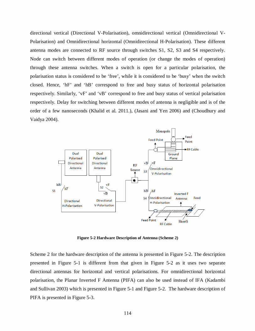
114

directional vertical (Directional V-Polarisation), omnidirectional vertical (Omnidirectional V-

Polarisation) and Omnidirectional horizontal (Omnidirectional H-Polarisation). These different

antenna modes are connected to RF source through switches S1, S2, S3 and S4 respectively.

Node can switch between different modes of operation (or change the modes of operation)

through these antenna switches. When a switch is open for a particular polarisation, the

polarisation status is considered to be ‘free’, while it is considered to be ‘busy’ when the switch

closed. Hence, ‘hF’ and ‘hB’ correspond to free and busy status of horizontal polarisation

respectively. Similarly, ‘vF’ and ‘vB’ correspond to free and busy status of vertical polarisation

respectively. Delay for switching between different modes of antenna is negligible and is of the

order of a few nanoseconds (Khalid et al. 2011.), (Jasani and Yen 2006) and (Choudhury and

Vaidya 2004).

Figure 5-2 Hardware Description of Antenna (Scheme 2)

Scheme 2 for the hardware description of the antenna is presented in Figure 5-2. The description

presented in Figure 5-1 is different from that given in Figure 5-2 as it uses two separate

directional antennas for horizontal and vertical polarisations. For omnidirectional horizontal

polarisation, the Planar Inverted F Antenna (PIFA) can also be used instead of IFA (Kadambi

and Sullivan 2003) which is presented in Figure 5-1 and Figure 5-2. The hardware description of

PIFA is presented in Figure 5-3.

115

Figure 5-3 Hardware Description of PIFA Antenna(Kadambi and Sullivan 2003)

To support the proposed dual polarised communication, antenna can operate in modes belonging

to different polarisations (horizontal and vertical) simultaneously. Therefore, simultaneous

directional or omnidirectional communication can take place over orthogonal polarisations.

However, at a given time, only one mode (directional or omnidirectional) in a particular

polarisation is used. Therefore, at a given time either omnidirectional or directional operation can

take place in vertical polarisation; and same holds true for operation over horizontal polarisation.

This is to avoid interference between directional or omnidirectional communication over same

polarisation.

In the proposed protocol, the broadcast packets such as Link ID and RREQ are transmitted and

received omnidirectionally to avoid circular directional or multidirectional transmission of

broadcast packets (which are meant for all the neighbour nodes of the transmitter). This is

because circular directional or multidirectional transmission of broadcast packets will lead to

increased overhead, because with 8 beams in switched beam antenna, copies same packet will

need to be transmitted 8 times (once over every beam) (Takata, Bandai and Watanbe 2005). For

omnidirectional exchange of packets, only vertically polarised omnidirectional antenna is used

because vertically polarised omnidirectional antennas are easy to realize when compared to

horizontally polarised omnidirectional antennas (Quan et al. 2012). Between omnidirectional

horizontal polarisation and directional horizontal polarisation, there are very limited designs

which give horizontally polarised omnidirectional antenna (Quan et al. 2012). Scarcity of designs

for horizontally polarised omnidirectional antenna is the reason for not choosing horizontally


116

polarised directional antennas for data communication. In this work, the horizontally polarised

omnidirectional antenna is used only for sensing the medium in horizontal polarisation.

Packets such as RTS, CTS, Data, ACK, RREP and RRER which are meant for particular nodes

are exchanged directionally among concerned nodes. Directional transmission allows to take

advantage of reduced interference and exposed node problem through directional communication

(Ramanathan et al. 2005), and (Nasipuri, Li, and Sappidi 2002), (Choudhary et al. 2002) and

(Takai et al. 2002). As nodes can simultaneously communicate over orthogonal channels, this

dual polarised directional communication also helps in alleviating the problems of deafness and

directional exposed nodes. The directional antennas considered for both the polarisations are

switched beam antennas comprising of eight beams (45° each, covering 360°). When idle (in

both the polarisations or in a particular polarisation), the antenna senses the medium in

omnidirectional mode accordingly (in both the polarisations, or in particular polarisation) as it

does not know the direction from which signal might arrive (Choudhury et al. 2002),(Choudhury

and Vaidya 2004), (Wang, Fang and Wu 2005) and (Subramanium and Das 2010). When a

signal is detected in omnidirectional mode in a particular polarisation, the antenna switches to

directional mode and performs azimuthal scan to determine the beam on which the impinging

signal is maximum (strength of the signal is maximum), and selects this beam to receive rest of

the signal (Subramanium and Das 2010) and (Choudhury and Vaidya 2004). To overcome the

problems arising due to asymmetry in gain (such as hidden terminals) discussed in (Choudhury

et al. 2002), (Subramanium and Das 2010) and (Abdullah, Cai, and Gebali 2012), the range and

gain of both directional and omnidirectional antennas is assumed to be same in (Nasipuri et al.

2000), (Huang et al. 2002), (Choudhury and Vaidya 2004), (Lee et al. 2006) and (Subramanium

and Das 2010). For operation of dual polarised directional communication discussed in this

thesis, the range of directional and omnidirectional communication is kept same to avoid

problems due to asymmetry in gains of (and thus communication range) directional and

omnidirectional communication.

5.2.2 Sequence of Transmission of Packets in DPDA-MAC

The sequence of frames exchanged between communicating nodes, and transmission of

intermediate broadcast packets is presented in Figure 5-4. As observed from Figure 5-4, Node A

117

transmits RTS frame to Node B directionally over the selected polarisation (based on the

information available in NT), to initiate communication with Node B. Appropriate polarisation is

selected by the node based on the information available in its NT. In order to receive the RTS

frame from Node A, Node B should be sensing the medium omnidirectionally in the same

polarisation, as used by Node A for transmission. On receiving RTS from Node A, Node B waits

for SIFS duration of 10µs and responds with CTS frame. The CTS frame is transmitted

directionally to Node A, using same polarisation on which RTS was received.

After exchange of CTS frame, the communication link is considered to be established between

the two nodes (Nodes A and B) on the selected polarisation. To inform other nodes about this

established link, Nodes A and B omnidirectionally transmit broadcast packet carrying Link ID

information in vertical polarisation. Both the nodes wait for DIFS duration of 50µs and some

random time as given in Equation 4.1 and Equation 4.2 of Chapter 4, before transmitting the

broadcast packet omnidirectionally in vertical polarisation. The method of broadcasting,

handling corruption of broadcast packets and contents of the broadcast packet are as explained in

Section 4.3 of Chapter 4. Since RTS and CTS frames are exchanged directionally, these

broadcast packets play an important role in informing neighbouring nodes about ongoing

communication. This helps in mitigating the problem of deafness, while exploiting the benefits

of directional communication. Information in these broadcast packets is used by other nodes to

update their NTs and NAV time. After the transmission of broadcast packet, Node A waits for

SIFS duration of 10µs and transmits the Data packet directionally to Node B. Node B also waits

for SIFS duration of 10µs before acknowledging the reception of Data packet through directional

transmission of acknowledgement to Node A. At the end of the exchange of RTS, CTS, Data

and ACK frames, both the nodes again transmit broadcast packet to inform neighbour nodes

about the end of communication. Before transmitting the broadcast packets, nodes wait for DIFS

duration and random time as given in Equation 4.1 and Equation 4.2. To indicate the end of

ongoing communication, the polarisation over which the communication was taking place is

represented as free, the NAV time of the concerned polarisation is changed to Zero and nodes are

shown as idle nodes in the NT.

118

Figure 5-4Sequence of Packet Transmission in DPDA-MAC

The broadcast frame is always transmitted omnidirectionally over vertical polarisation. All the

other frames such as RTS, CTS, Data and ACK, are transmitted directionally over the selected

polarisation. Before RTS transmission, Node A first waits for the medium to be idle. On sensing

the medium to be idle, it waits for DIFS and random time. The random waiting time is based on

the contention window. This time is represented by Equation 4.1.On receiving RTS, Node B

waits for SIFS duration of 10µs and transmits CTS. While Nodes A and B communicate in one

polarisation, other nodes which are within the communication range of Nodes A and B, wait for

the ongoing communication in that polarisation to end by waiting for NAV duration, before

trying to access the medium. However, if other orthogonal polarisation is available, other nodes

within the communication range of Node A and / or B can communicate in the available

orthogonal polarisation simultaneously in order to exploit the benefits of dual polarisation.

5.2.3 Flowchart for DPDA-MAC

In DPDA-MAC, all the communication links use dual polarised directional antennas. Main aim

of DPDA-MAC is to overcome interference, exposed node problem, directional exposed node

119

problem and deafness in MANETs. When idle, nodes sense the medium omnidirectionally in

both horizontal and vertical polarisations. Broadcast packets are exchanged using

omnidirectional antenna with vertical polarisation. RTS, CTS, Data and ACK packets are

exchanged using directional antenna with appropriate polarisation. Appropriate polarisation is

selected based on multiple factors such as, available polarisation at next hop node, available

polarisation at the source and polarisation being used by neighbour nodes so that orthogonal

polarisation can be used to reduce interference and directional exposed node problem. In case

both the polarisations are available, use of horizontal polarisation is preferred for exchange of

RTS, CTS, Data and ACK frames, in order to avoid interference with broadcast packets which

are exchanged using omnidirectional antenna with vertical polarisation. In case the source node

does not find the required polarisation to be free at the transmitter, then it either waits for the

polarisation to be free at the transmitter based on the NAV time, or it checks if it can initiate

communication over other available polarisation. In case, both the polarisations are not available

for communication, the source node has no choice, but to wait based on NAV information. The

only requirement of DPDA-MAC is that two nodes should be able to use same polarisation to

initiate communication with each other. The flowchart for DPDA-MAC based communication of

transmitter and receiver nodes is shown in Figure5-5, Figure 5-6 and Figure 5-7.The flowchart

for transmission of Broadcast, RTS, CTS, Data and ACK packets, in DPDA-MAC is presented

in Figure5-5 and Figure 5-6. The detailed explanation of the flowchart is as follows.

Exchange Broadcast Packets and Form NT:

Initially, all the nodes exchange broadcast packets, using vertically polarised omnidirectional

antenna. The contents of broadcast packets are explained in Chapter 4. The details about

transmission of broadcast packets and method to handle corruption of packets among them are

also given in Chapter 4. These broadcast packets are used to maintain NT, an example for which

is presented in Table 4-1 of Chapter 4. All the nodes constantly transmit broadcast packets to

inform their neighbour nodes regarding communicating or idle nodes, free or busy polarisation,

NAV time, location information and RSSI. Nodes within the communication range of each other,

maintain a NT in the network layer. Based on this information, the MAC layer decides about the

appropriate polarisation over which required communication can be initiated.

120

Data Transmission:

Initially, if a node is not participating in communication, it continues to sense the network

omnidirectionally in both vertical and horizontal polarisations. This enables the node to receive

communication requests from other nodes from any direction and in any polarisation, when both

the polarisations of the node are free. Omnidirectional sensing of network takes place only over

the polarisation which is free (not being used for directional communication with other node). In

DPDA-MAC, based on the information available in the NT about the next hop, appropriate

polarisation is chosen to directionally transmit the Request-To-Send (RTS) packet to the next

hop node. When a node needs to transmit data to another node in the network which is not in

direct communication range of the source node, the network layer initiates a route discovery

process for establishing a route with the desired destination node. For this, the neighbour nodes

form prospective next hop nodes to establish a route to communicate with the required node. The

process of route discovery and maintenance is carried out according to the Dual Polarised

Directional Antenna based Multipath Routing Protocol (DPDA-MRP), which is explained in

Chapter 6.

Choose Appropriate Polarisation:

DPDA-MAC deals with the communication between two neighbour nodes. Based on the

information available in the NT, transmitter node chooses appropriate polarisation to initiate

communication with the receiver node. The transmitter checks for free polarisation available

with itself and the intended next hop receiver. For this communication, antenna polarisation for

both the communicating nodes must be same.

Chosen Polarisation Available?:

If the transmitter does not find same polarisation to be free at the receiver, it waits for NAV time

for the desired polarisation to be available. It must be noted that, as vertical polarisation is used

for transmission of broadcast packets, in case of availability of both the polarisations, horizontal

polarisation is preferred for data communication in order to avoid interference with broadcast

packets exchanged in vertical polarisation.

121

Tx RTS Using <Pol>:

The chosen polarisation is represented as <Pol> in the flowchart of Figure5-5 and Figure 5-6.

Once appropriate polarisation is chosen, the transmitting node transmits RTS frame directionally

to the intended receiver. The location information available in the NT is used to direct the beam

in the direction of receiver. Since the chosen polarisation is free at the intended receiver, the

receiver should be sensing the medium omnidirectionally in that polarisation, and should be

ready to receive communication request from any direction.

Wait for CTS in <Pol> or Timeout:

After RTS transmission in <Pol>, the transmitter transits to omnidirectional mode to receive the

CTS frame. It senses the medium omnidirectionally in <Pol> for CTS. If the CTS frame is not

received before Timeout period of 110 ms, RTS is retransmitted. The sender tries to retransmit

the RTS frame 5 times. If retransmission limit of 5 tries is reached without receiving CTS, the

transmitter aborts the transmission. It also updates the network and application layers about

aborting the transmission. The node then starts sensing the medium omnidirectionally with now

available polarisation.

Broadcast Link ID Information:

If CTS is received, the establishment of communication link is confirmed. At this point, the

transmitter sends broadcast packet showing <Pol> as busy with specific NAV time and node

with which it is communicating. This makes other neighbour nodes aware of the ongoing

communication and polarisation usage of the nodes. Transmission of this broadcast message

helps in avoiding the problem of deafness at the nodes near the transmitter.

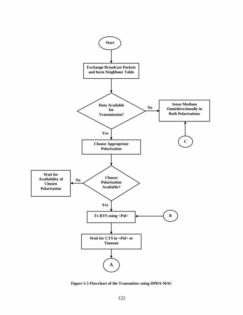
122

Figure 5-5 Flowchart of the Transmitter using DPDA-MAC

Start

Exchange Broadcast Packets and form Neighbour Table

Data Available for

Transmission?

Sense Medium Omnidirectionally in

Both Polarisations

C

No

Choose Appropriate Polarisation

Yes

Chosen Polarisation Available?

No Wait for

Availability of Chosen

Polarisation

Yes

Tx RTS using <Pol>

Wait for CTS in <Pol> or Timeout

A

B

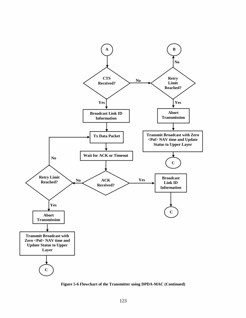
123

Figure 5-6 Flowchart of the Transmitter using DPDA-MAC (Continued)

A B

CTS Received?

Yes

Broadcast Link ID Information

Tx Data Packet

Wait for ACK or Timeout

ACK Received?

No Retry Limit Reached?

Abort Transmission

Transmit Broadcast with Zero <Pol> NAV time and

Update Status to Upper Layer

C

Yes

No

Yes Broadcast Link ID

Information

C

Retry Limit

Reached?

No

Yes

Abort Transmission

Transmit Broadcast with Zero <Pol> NAV time and Update

Status to Upper Layer

No

C

124

Tx Data:

After broadcasting Link ID information, the node directionally transmits data to the receiver

using <Pol>. Before data transmission the node waits for SIFS duration of 10 µs.

Wait for ACK or Timeout:

After directional transmission of data frame over <Pol>, the node transits to omnidirectional

mode in <Pol>and waits for acknowledgement. If the acknowledgement does not arrive till

timeout of 110ms, the node retransmits the data frame. If acknowledgment is not received even

after retransmission limit of 5 is reached, the node aborts the communication.

On aborting the transmission, node updates the upper layers (network and application layers)

about the same. It also transmits broadcast packet omnidirectionally with Zero <Pol> NAV to

inform its neighbour nodes about the availability of <Pol>. This information can be used by

other nodes that wish toinitiate communication with this node. After this, the node switches to

omnidirectional mode and starts sensing the medium for further RTS requests and broadcast

packets.

Flowchart of the Receiver:

The flowchart for the receiver node is presented in Figure 5-7. Different stages in the flowchart

are explained as follows.

Sense medium omnidirectionally in both polarisations:

When a node is idle, it senses the medium omnidirectionally, in that polarisation. Significance of

omnidirectional sensing is to make the node capable of receiving the connection requests from

other nodes in any direction, because the requests are transmitted directionally.

Once the node receives RTS packet on <Pol> from other node, it changes to directional mode to

transmit the CTS frame in the same <Pol>,after SIFS duration of 10 µs.

125

Figure 5-7Flowchart of the Receiver for DPDA-MAC

Start

Sense Medium Omnidirectionally in

Both Polarisations

Received RTS?

Transmit CTS using <Pol>

Yes

No

Transmit Broadcast with Zero <Pol> NAV

time

Tx ACK Data Received?

Broadcast Link ID Information

Wait for Data in <Pol> or Timeout

Retry Limit Reached?

No

No Yes

Transmit Broadcast with Zero <Pol> NAV time and

Update Status to Upper Layer

Yes

126

Transmit CTS using <Pol>:

The node stays in omnidirectional mode till it receives the RTS frame for establishment of

communication link. On receiving the RTS frame on a particular polarisation, it waits for SIFS

duration of 10µs and then transmits CTS frame directionally over the same polarisation to

confirm the establishment of communication link over chosen polarisation with the transmitter of

RTS frame.

Broadcast Link ID Information:

On confirming the establishment of communication link, the receiver node broadcasts Link ID

information omnidirectionally in vertical polarisation after the DIFS duration of 50µs and

random backoff. The Link ID information primarily conveys information about <Pol> busy

status, NAV duration and node with which link is established to the neighbour nodes. This

transmission of the broadcast frame informs the neighbour nodes of the receiver about ongoing

communication in order to avoid deafness at the other nodes.

Wait for Data in <Pol> or Timeout:

After broadcast of Link ID information, the node senses the medium omnidirectionally to receive

data packet by the transmitter. Reception always takes place omnidirectionally as the transmitter

may be mobile and data packet can arrive from any direction.The receiver node waits for the data

packet for a timeout of 110ms. In case timeout is reached; the CTS frame is retransmitted till

retransmission limit of 5 times is over. On receiving the data packet, the receiver node transmits

an acknowledgement frame to the transmitter of data packet. However, if the retransmission limit

is also reached, but data packet does not arrive, the receiver node broadcasts Link ID information

indicating availability of polarisation and NAV duration as Zero.

If data packet does not arrive:

If data packet does not arrive even after retransmission limit for CTS frame is reached, the

receiver considers it to be a broken connection and frees the <Pol>. In order to inform neighbour

nodes about the same, it broadcasts Link ID information with <Pol> as free and NAV time

asZero. The node also updates the upper layers (network and application) about the status.After

127

the polarisation becomes free, the node transits to omnidirectional mode and starts sensing the

medium to receive new communication requests on freed polarisation.

If data packet is received:

On reception of data packet from the transmitter, the receiver node transmits ACK directionally

on <Pol> to the transmitter after SIFS duration of 10µs. After transmission of ACK, the receiver

waits for DIFS duration of 50µs and random backoff, and broadcasts the Link ID information

indicating free <Pol> and Zero NAV time to inform other nodes about completion of

communication. After completion of communication among the nodes, like the transmitter,

receiver node also transits to omnidirectional mode and starts medium sensing to receive new

communication requests on freed polarisation. The timeout values for different frames are listed

in Table 5-1, as follows:

Table 5-1 Timeout Values for Different Frames

SIFS 10µs

DIFS 50µs

ACK Timeout at sender 110ms

CTS Timeout at sender 110ms

Maximum retransmission count 5

In case of corruption of broadcast packets, they are retransmitted with random backoff, at the

occurrence of Corruption Detection Pulse (CDP). The random backoff that each node undergoes

is Equation 4.1 and Equation 4.2 of Chapter 4. It must be noted that all the communication links

use directional antennas, and communication can take place simultaneously in both vertical and

horizontal polarisations. In idle state, nodes sense the medium in omnidirectional mode in both

vertical and horizontal polarisations. Broadcast packets are exchanged over omnidirectional

antenna with vertical polarisation. RTS, CTS, Data and ACK packets are exchanged using

directional antenna with appropriate polarisation. Appropriate polarisation is selected based on

multiple factors such as, available polarisation at the next hop destination, available polarisation

at the source, polarisation being used by neighbour nodes so that opposite polarisation can be

used to reduce interference and overcome directional exposed node problem. In case both the

polarisations are available, use of horizontal polarisation is preferred for exchange of RTS, CTS,

128

Data and ACK frames. This is to avoid interference with broadcast packets which are exchanged

using omnidirectional antenna with vertical polarisation. In case the source node does not find

the required polarisation to be free at the transmitter, then it either waits for the polarisation to be

free at the transmitter based on the NAV time, or it checks if it can initiate communication over

other available polarisation. In case, both the polarisations are not available for communication,

the source node has no choice, but to wait based on NAV information present in its NT. The only

requirement of DPDA-MAC is that two nodes should be able to use same polarisation to initiate

communication with each other.

5.3 Avoidance of Directional Exposed Node and Deafness with DPDA-MAC

As observed from the literature survey, the exposed node problem exists even in the presence of

directional antenna. This section explains how the exposed node problem present even with the

use of directional antenna can be alleviated by using DPDA-MAC by the virtue of dual

polarisation.

Figure 5-8Directional Exposed Node Problem Avoidance with DPDA-MAC

As discussed earlier, broadcast packets are exchanged among nodes to establish NT. The

contents of the broadcast packet include polarisation information about free and busy

polarisations of neighbour nodes, NAV duration at both vertical and horizontal polarisations, and

location of the transmitting node, among other parameters shown in Table 4-1. This information

is used by the nodes to choose appropriate polarisation in order to minimise interference and

mitigate the exposed node problem. It is assumed that all the nodes in the network use antenna

having same gain, therefore communication range of all the nodes remains fixed. From the

information available in the NT, a node can determine its location with respect to its neighbours,

and polarisation related information of the concerned nodes.

129

In the example illustrated in Figure 5-8, Nodes A and B communicate using horizontal

polarisation. Node C, which is present within the communication range of Nodes A and B gets

affected due to NAV on horizontal polarisation because of ongoing communication between

Nodes A and B. Therefore, it chooses to use vertical polarisation to initiate communication with

Node D. This way, simultaneous communication between two different pairs of nodes takes

place without any node being exposed due to other’s communication.

It must be observed that this method of dual polarisation to mitigate the exposed node problem

can also be used when nodes communicate using omnidirectional antenna. However, in this case,

the advantage of spatial reuse provided by the use of directional antennas cannot be utilised.The

problem of deafness, which occurs due to the use of directional antenna can also be handled with

the use of DPDA-MAC. According to DPDA-MAC, the nodes which communicate using

directional antenna broadcast the Link ID information conveying their busy status along with the

polarisation in use immediately after the exchange of RTS-CTS frames. The nodes which are the

neighbours of the communicating nodes become aware of busy or free polarisations through

these broadcasts. Based on the information available in Link ID frame, neighbour nodes

receiving the broadcast can either decide to use the polarisation that is free or wait for the busy

polarisation to become free.

Figure 5-9Deafness Avoidance with DPDA-MAC

The example of avoidance of deafness with the use of DPDA-MAC protocol is presented in

Figure 5-9. In the example shown in Figure 5-9, Nodes A and B communicate using vertical

polarisation. With the broadcast of Link ID information, Node A conveys the busy status of its

vertical polarisation as well as corresponding NAV duration. Since horizontal polarisation of

Node A is free, it senses the medium omnidirectionally in horizontal polarisation. Through Link

ID broadcast from Node A, Node C gets to know that horizontal polarisation of Node A is free.

Therefore, Node C directionally transmits RTS to Node A in horizontal polarisation. After

successfully receiving directional RTS from Node C, Node A transmits CTS frame to Node C in

130

the same polarisation. Thus connection is established between Nodes A and C in spite of Node A

being busy in communicating with Node B, thereby avoiding the occurrence of deafness.

It is to be noted that while DPDA-MAC helps in dealing with the problem of directional exposed

node and deafness, it does not completely eliminate these problems. Since, there are only two

orthogonal polarisations available to be used for simultaneous communication, for one

directional beam, only one more node can be benefitted with avoidance of deafness. For the

avoidance of directional exposed node, as long as nodes utilise the available orthogonal

polarisations such that they do not interfere with each other, nodes get benefitted with the use of

dual polarised directional antenna.

5.4 Results and Discussion

This section presents the results obtained through simulations carried out to study the

performance of three MAC layer protocols namely Dual Polarised Directional Antenna based

Medium Access Control (DPDA-MAC), Single Polarised Directional Antenna based Medium

Access Control (SPDA-MAC) and Carrier Sense Multiple Access / Collision

Avoidance(CSMA/CA). In order to appreciate the importance of using dual polarised directional

communication to enhance performance of the network, it is important to compare the

performance of communication carried out using dual polarised directional antenna with that

carried out using single polarised directional antenna and omnidirectional communication over

single polarisation.

Detailed explanation of design and functionality of DPDA-MAC is given in Section 5.2. The

operation of SPDA-MAC protocol is similar to that of DPDA-MAC protocol except that in

SPDA-MAC protocol nodes use only vertical polarisation for directional communication. Like in

DPDA-MAC, in SPDA-MAC also nodes exchange periodic Link ID broadcasts to maintain NT.

This helps in overcoming the problem of deafness while carrying out directional communication.

However, the use of only one polarisation in SPDA-MAC provides only one channel for

communication. This can adversely affect the throughput of the network because of the absence

of simultaneous communication over orthogonal polarisations. Also, the problem of directional

exposed node (explained in Section 2.6.6) persists with SPDA-MAC due to non availability of

orthogonal polarisation, unlike DPDA-MAC. The sequence of exchange of RTS, CTS, Data and

131

ACK frames along with exchange of intermediate broadcasts in SPDA-MAC is same as that of

DPDA-MAC (shown in Figure 5-4).

The IEEE 802.11 standard uses CSMA/CA as the method to access the wireless medium.

CSMA/CA uses omnidirectional antenna for communication and is explained in Section 2.6.3 of

Chapter 2. Due to the use of omnidirectional antenna over single polarisation, nodes experience

higher instances of problems of exposed nodes and interference when compared those faced with

the use of dual polarised directional antenna.

Since the DPDA-MAC, SPDA-MAC and CSMA/CA protocols deal with accessing the wireless

medium to communicate with the next hop node, the performance of these three protocols is

studied for single hop communication. The simulation results present the performance of these

three MAC layer protocols in terms of throughput and per-hop delay. When performance is

studied for single hop communication, it is observed that all the packets successfully get

transmitted to the next hop within given simulation time. This leads to PDR of 100% for all cases

and all three protocols. Therefore, results for PDR are not plotted.

The significance of this study is to analyse and compare the performance of DPDA-MAC,

SPDA-MAC and CSMA/CA as all these MAC layer protocols have different characteristics.

DPDA-MAC is capable of avoiding the problem of deafness with use of dual polarised

communication and broadcast of Link ID packets. DPDA-MAC uses directional communication

which helps in reducing the instances of nodes undergoing the problem of exposed node. Nodes

may also experience the problem of directional exposed node (explained in Section 2.6.6), which

can be reduced by DPDA-MAC through the use of dual polarisation. SPDA-MAC carries out

directional communication over single polarisation. Therefore, while SPDA-MAC reduces the

number of nodes undergoing the problem of exposed node, it cannot avoid nodes from

experiencing the problem of directional exposed nodes (explained in Section 2.6.6). SPDA-MAC

also broadcasts Link ID information to its neighbour nodes in order to avoid deafness, however,

nodes cannot take advantage of dual polarisation to carry out simultaneous communication over

orthogonal polarisations with two different nodes. CSMA/CA is IEEE 802.11 based method for

accessing the medium. It carries out communication omnidirectionally in single polarisation;

132

therefore, while nodes do not experience the problem of deafness, they undergo the problem of

exposed node. Since communication is carried out over single polarisation only, CSMA/CA

cannot exploit advantages of simultaneous communication over orthogonal communication

channels with the use of dual polarised communication. These different characteristics of DPDA-

MAC, SPDA-MAC and CSMA/CA result in difference of throughput and per-hop delay

achieved by these protocols. This simulation study is aimed at analysing the difference in

throughput and per-hop delay achieved by DPDA-MAC, SPDA-MAC and CSMA/CA at

different values of node mobility, node density and channel capacity.

Simulations are carried out in a simulator developed in C++.The details of the developed

simulator are presented in Appendix 1.The specifications for MANET scenarios used for this

study are given in Table 5-2. Simulations are carried out to study and compare the performance

of DPDA-MAC, SPDA-MAC and CSMA/CA protocols used for access to wireless medium in

MANETs. The nodes in simulated MANET scenarios are placed on a terrain of size 1000x1000

m2. The number of nodes placed in this terrain are varied while keeping the size of the terrain

same, to achieve different values of node density.

The simulations are carried out for different values of node density with 20, 40, 60, 80 and 100

nodes placed per unit area. For a given value of node density, 25% of the total nodes are the

transmitters and another 25% of total nodes are the receivers. Therefore, for 20, 40, 60, 80 and

100 nodes, the number of transmitters and receivers are 5, 10, 15, 20 and 25 respectively.

Therefore, while 50% of the nodes in the network act as source and sink and information, other

nodes can help in routing of information between the communicating nodes. The nodes in the

simulated MANET scenario are placed in random topology and move based on random waypoint

mobility model. The simulations are carried out over values of node mobility being 0 m/s

(stationary nodes), 1 m/s, 2 m/s and 3 m/s with a pause time of 4 s to simulate walking and

running speed of humans. Simulations are carried out for 50 seeds and average of 50 runs is

taken to plot the graphs for different performance parameters. The rate of packet transmission is

varied as 1, 5, 15 and 25 packets per second where each packet carries 1024 Bytes.

133

Table 5-2Scenario Specifications for Performance Analysis of MAC Protocols

Parameter Value

Terrain Size 1000 x 1000 m2

Number of Nodes 20, 40, 60, 80 and 100

Number of Transmitters 05, 10, 15, 20 and 25

(25% of total number of nodes)

Number of Receivers 05, 10, 15, 20 and 25


Node Placement Random

MAC Protocol DPDA-MAC, SPDA-MAC,

CSMA/CA

Node Mobility Random Waypoint

Speed 0, 1, 2, 3 m/s

Pause Time 4s


Packets Per Second 1, 5, 15, 25

Channel Capacity 2, 11 and 54 Mbps

Probability of Error 5%

Simulation Time 100s

Communication Range 200m

Threshold SNR 10 dB

Number of Seeds 50

The rate of packet transmission is increased to study the effect of increase in network load on the

performance on the network. As stated in Section 3.2 of Chapter 3, nodes configured to 802.11

can have transmission range of up to 250 m. However, the range of communication maintained

between the nodes in the simulated scenario is 200m only because channel orthogonality is

maintained for a maximum distance of 200 m only in Line Of Sight (LOS) settings for ad-hoc

networks (Khalid et al. 2011). In practice, the threshold SNR in MANETs is usually set to 10 dB

(Xu, Gerla and Bae 2003). Therefore, threshold SNR of 10 dB is configured for the simulated

scenario. The simulations are carried out for values of channel capacity being 2, 11 and 54 Mbps

(Burton 2009), and probability of error being 5% (Halford and Chugg 2011), (Theodore and

134

Fidelis 2013) and (Hayajneh et al., 2009). Random waypoint mobility model is used because it is

the most popular and frequently used mobility model used in simulation based studies of

MANETs (Bai and Helmy 2004) and (Bettstetter and Wagner 2002).

5.4.1 Effect of Variation in Density and Mobility of Nodes on Throughput Achieved

by DPDA-MAC, SPDA-MAC and CSMA/CA with Varying Rate of Packet

Transmission

Throughput is computed as the number of bits received successfully by the node which is one

hop away from the transmitting node, over the duration of simulation. This section presents the

results and their analysis for throughput achieved by DPDA-MAC, SPDA-MAC and CSMA/CA.

Simulations are carried out based on the specifications given in Table 5-2. Node mobility is an

essential characteristic of MANETs and must be considered while analysing their performance.

Therefore, this study is carried out for different values of mobility of nodes to simulate walking

and running speed of humans. Density of nodes is varied to study the effect of exposed nodes on

the performance of DPDA-MAC, SPDA-MAC and CSMA/CA. Rate of packet transmission and

capacity of channel are essential parameters influencing the performance of a wireless network.

Therefore, this study is carried out for different rates of packet transmission and different values

of channel capacity. The results are plotted along with standard deviation for all the three

protocols.

5.4.1.1 Analysis of the Variation in Throughput of DPDA-MAC

In this section, variation in throughput of the network is studied when DPDA-MAC is used as

the MAC protocol to communicate with next hop node. DPDA-MAC carries out directional

communication over orthogonal polarisations. For this study, the density of nodes is varied from

20 nodes per unit area to 100 nodes per unit area, in steps of 20. Mobility of nodes is varied from

0 m/s (stationary nodes) to 3 m/s in steps of 1 m/s. Throughput is measured for different channel

capacities of 2 Mbps, 11 Mbps and 54 Mbps.

Throughput of DPDA-MAC with Rate of Packet Transmission being 1 Packet per Second

Variation in throughput achieved by DPDA-MAC is studied by varying density and mobility of

nodes. Simulations are carried out for channel capacities of 2 Mbps, 11 Mbps and 54 Mbps,

when rate of packet transmission is 1 packet per second.

135

Variation in throughput is presented for node mobility values of 0 m/s (stationary nodes), 1 m/s,

2 m/s and 3 m/s (Figure 5-10a, b, c and d). From the simulations it is observed that throughput

increases almost linearly with increase in density of nodes. When nodes move at the 3 m/s

throughput with node density of 20 nodes per unit area is 33 kbps and it increases to 177 kbps

with increase in node density to 100 nodes per unit area (Figure 5-10d).

Figure 5-10 Variation in Throughput with Node Density at Different Values of Node Mobility for DPDA-

MAC at1 Packet per Second

Throughput of DPDA-MAC with Rate of Packet Transmission being 5 Packets per Second

Throughput achieved when rate of packet transmission is increased to 5 packets per second is

presented in Figure 5-11. Variation in throughput is presented for different values of node

mobility in Figure 5-11a, b, c and d. When the nodes are stationary (Figure 5-11a), throughput

with 20 nodes per unit area is 182.7 kbps and increases to 907.6 kbps with 100 nodes per unit

(a) (b)

(c) (d)

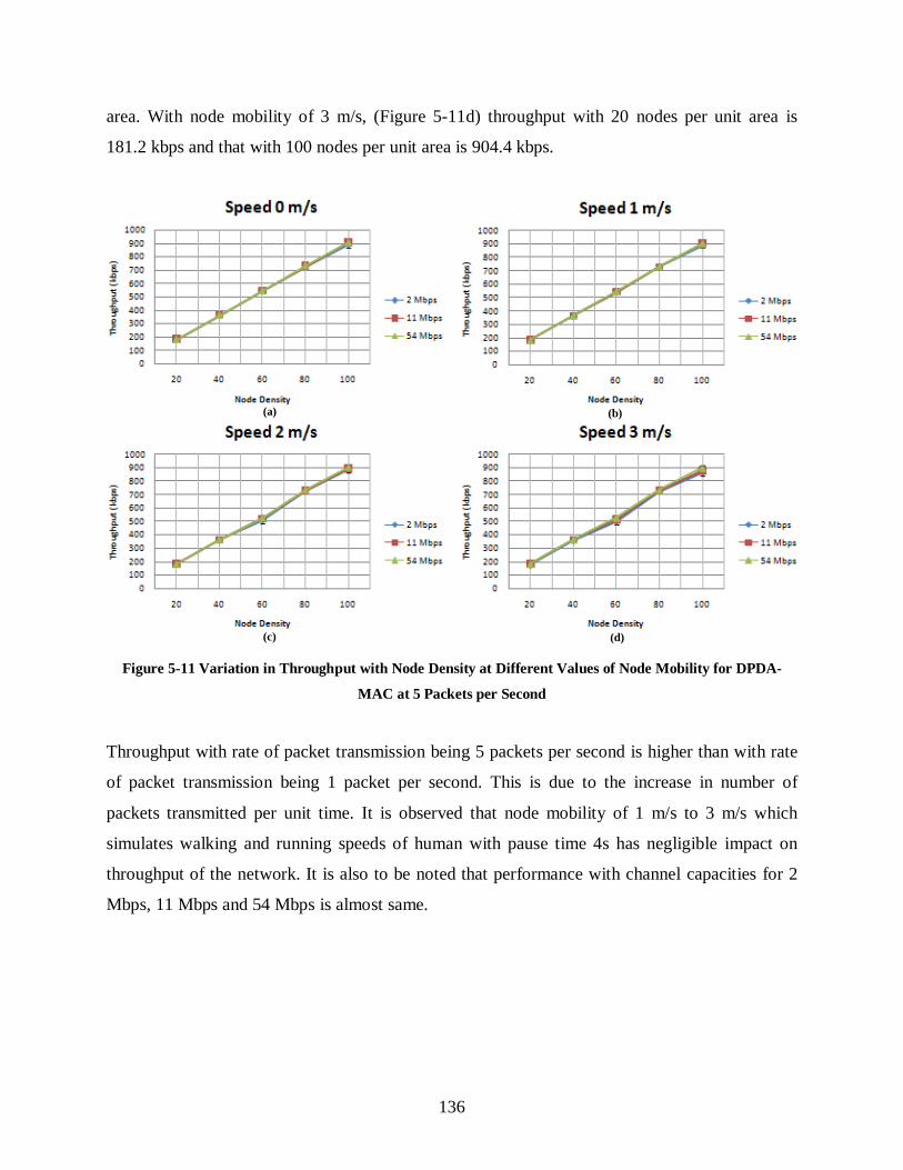
136

area. With node mobility of 3 m/s, (Figure 5-11d) throughput with 20 nodes per unit area is

181.2 kbps and that with 100 nodes per unit area is 904.4 kbps.


MAC at 5 Packets per Second

Throughput with rate of packet transmission being 5 packets per second is higher than with rate

of packet transmission being 1 packet per second. This is due to the increase in number of

packets transmitted per unit time. It is observed that node mobility of 1 m/s to 3 m/s which

simulates walking and running speeds of human with pause time 4s has negligible impact on

throughput of the network. It is also to be noted that performance with channel capacities for 2

Mbps, 11 Mbps and 54 Mbps is almost same.

(a) (b)

(c) (d)

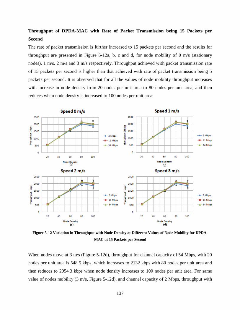
137

Throughput of DPDA-MAC with Rate of Packet Transmission being 15 Packets per

Second

The rate of packet transmission is further increased to 15 packets per second and the results for

throughput are presented in Figure 5-12a, b, c and d, for node mobility of 0 m/s (stationary

nodes), 1 m/s, 2 m/s and 3 m/s respectively. Throughput achieved with packet transmission rate

of 15 packets per second is higher than that achieved with rate of packet transmission being 5

packets per second. It is observed that for all the values of node mobility throughput increases

with increase in node density from 20 nodes per unit area to 80 nodes per unit area, and then

reduces when node density is increased to 100 nodes per unit area.



When nodes move at 3 m/s (Figure 5-12d), throughput for channel capacity of 54 Mbps, with 20

nodes per unit area is 548.5 kbps, which increases to 2132 kbps with 80 nodes per unit area and

then reduces to 2054.3 kbps when node density increases to 100 nodes per unit area. For same

value of nodes mobility (3 m/s, Figure 5-12d), and channel capacity of 2 Mbps, throughput with

(a) (b)

(c) (d)

138

20 nodes per unit area is 546.6 kbps, which increases to 2012.2 kbps for 80 nodes per unit area,

and drops to 1868.4 kbps when node density is increased to 100 nodes per unit area.

Throughput of DPDA-MAC with Rate of Packet Transmission being 25 Packets per

Second

Rate of packet transmission is further increased to 25 packets per second and obtained

throughput is presented in Figure 5-13.



Throughput obtained with transmission rate of 25 packets per second is higher than that obtained

with transmission rate of 15 packets per second. It is observed that variation in mobility of nodes

does not affect the performance drastically.

(a) (b)

(c) (d)

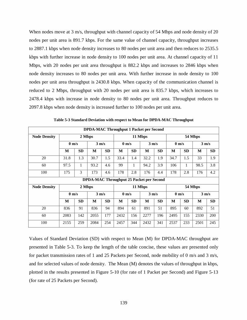
139

When nodes move at 3 m/s, throughput with channel capacity of 54 Mbps and node density of 20

nodes per unit area is 891.7 kbps. For the same value of channel capacity, throughput increases

to 2887.1 kbps when node density increases to 80 nodes per unit area and then reduces to 2535.5

kbps with further increase in node density to 100 nodes per unit area. At channel capacity of 11

Mbps, with 20 nodes per unit area throughput is 882.2 kbps and increases to 2846 kbps when

node density increases to 80 nodes per unit area. With further increase in node density to 100

nodes per unit area throughput is 2430.8 kbps. When capacity of the communication channel is

reduced to 2 Mbps, throughput with 20 nodes per unit area is 835.7 kbps, which increases to

2478.4 kbps with increase in node density to 80 nodes per unit area. Throughput reduces to

2097.8 kbps when node density is increased further to 100 nodes per unit area.

Table 5-3 Standard Deviation with respect to Mean for DPDA-MAC Throughput

DPDA-MAC Throughput 1 Packet per Second

Node Density 2 Mbps 11 Mbps 54 Mbps

0 m/s 3 m/s 0 m/s 3 m/s 0 m/s 3 m/s


20 31.8 1.3 30.7 1.5 33.4 1.4 32.2 1.9 34.7 1.5 33 1.9

60 97.5 1 93.2 4.6 99 1 94.2 3.9 106 1 98.5 3.8

100 175 3 173 4.6 178 2.8 176 4.4 178 2.8 176 4.2

DPDA-MAC Throughput 25 Packet per Second


0 m/s 3 m/s 0 m/s 3 m/s 0 m/s 3 m/s


20 836 91 836 94 894 61 891 51 895 60 892 51

60 2083 142 2055 177 2432 156 2277 196 2495 155 2330 200

100 2155 259 2084 254 2457 344 2432 341 2537 233 2501 245

Values of Standard Deviation (SD) with respect to Mean (M) for DPDA-MAC throughput are

presented in Table 5-3. To keep the length of the table concise, these values are presented only

for packet transmission rates of 1 and 25 Packets per Second, node mobility of 0 m/s and 3 m/s,

and for selected values of node density. The Mean (M) denotes the values of throughput in kbps,

plotted in the results presented in Figure 5-10 (for rate of 1 Packet per Second) and Figure 5-13

(for rate of 25 Packets per Second).

140

Following inferences can be drawn from the results presented in Figure 5-10 to Figure 5-13, and

Table 5-3

1. Throughput increases with increase in the rate of packet transmission. This is expected

because increase in rate of packet transmission leads to increase in the number of packets

propagated into the network

2. At lower rates of packet transmission (1 and 5 packets per second), throughput achieved

at channel capacities of 54 Mbps, 11 Mbps and 2 Mbps is almost same. This is because

when the rate of packet transmission is low (1 and 5 packets per second), channel

capacity of 2 Mbps is also sufficient to carry packets from one node to its next hop.

However, the effect of variation in channel capacity on performance becomes evident at

higher rates of packet transmission (15 and 25 packets per second). As observed from

obtained results, throughput achieved with channel capacity of 54 Mbps is highest and

that achieved with channel capacity of 2 Mbps is lowest

3. Throughput increases with increase in node density. This is because of the increase in the

number of transmitting and receiving nodes which increases the number of packets

exchanged over the network in a given time. This trend of increase in throughput with

increase in node density is observed for lower packet rates of 1 and 5 packets per second.

However, when the packet rates are increased to 15 and 25 packets per second,

throughput increases with increase in node density for up to certain value of node density

and then starts to drop when density of nodes is increased further. This is due to increase

in contention to access the medium and network congestion with increase in density of

nodes

4. Throughput does not change drastically with node mobility. In this scenario, nodes follow

random waypoint mobility model, according to which they move at speeds varying from

0 m/s (stationary nodes) to 3 m/s. For all these values of node mobility, pause time is 4s.

Apart from that, nodes periodically (every 1000ms), exchange Link ID information,

which carries location information of the broadcasting nodes. Based on this information

141

the transmitter can direct its beam towards the receiver without breaking the connection

due to node mobility. Therefore, the considered values of mobility of nodes which are

aimed to simulate walking and running speeds of humans do not affect the performance

of DPDA-MAC drastically for scenario specifications given in Table 5-2

5. From the values of Standard Deviation (SD) with respect to Mean (M) presented in Table

5-3it is seen that standard deviation increases with increase in traffic load on the network.

Traffic load on the network increases with increase in rate of packet transmission and

node density (which leads to increase in the number of communicating nodes).When

traffic load on the network is increased, more packets are exchanged over the shared

medium leading to more instances of random backoff delays among nodes trying to

access the medium. This leads to variation in the number of packets exchanged over the

medium for given duration of simulation. This causes the throughput across different

seeds to vary

6. Standard deviation is less in cases with less traffic load because in such cases medium is

capable of handling the given load and there are lesser instances of random backoff

among nodes to access the shared medium. In cases with lesser traffic load, variation of

throughput across different seeds is less and hence the standard deviation is less in such

cases.

5.4.1.2 Analysis of the Variation in Throughput of SPDA-MAC

This section presents the study and analysis of variation in throughput when SPDA-MAC is used

as the MAC protocol for communication between nodes which are one hop away from each

other. SPDA-MAC carries out directional communication over single polarisation. Results are

presented for different values of density and mobility of nodes, at channel capacity values of 2

Mbps, 11 Mbps and 54 Mbps. Different rates of packet transmission considered for this study are

1, 5, 15 and 25 packets per second, results for which are presented in Figure 5-14 to Figure 5-17

respectively. The density of nodes is varied from 20 nodes per unit area to 100 nodes per unit

area, in steps of 20. Node mobility is varied from 0 m/s (stationary nodes) to 3 m/s, in steps of 1

m/s.

142

Throughput of SPDA-MAC with Rate of Packet Transmission being 1 Packet per Second

The results for throughput of SPDA-MAC when packets are transmitted at a rate of 1 packet per

second are presented in Figure 5-14.

Figure 5-14 Variation in Throughput with Node Density at Different Values of Node Mobility for SPDA-

MAC at1 Packet per Second

From the results presented in Figure 5-14, it is evident that throughput increases with increase in

density of nodes, and variation in mobility of nodes has negligible effect on network

performance. Also, at low packet transmission rate of 1 packet per second, performance with

channel capacity of 2 Mbps is as good as that with channel capacity of 54 Mbps. When nodes

move at 3 m/s (Figure 5-14d) with channel capacity being 54 Mbps, throughput with 20 nodes

per unit area is 34 kbps, and increases to 174.5 kbps with increase in density of nodes to 100

nodes per unit area. This is almost same for different values of channel capacity and node

mobility.

(a) (b)

(c) (d)

143

Throughput of SPDA-MAC with Rate of Packet Transmission being 5 Packets per Second

The rate of packet transmission is further increased to 5 packets per second, and results for the

same are presented in Figure 5-15.

Figure 5-15 Variation in Throughput with Node Density at Different Values of Node Mobility for SPDA-


It is observed that throughput with packet transmission rate of 5 packets per second is higher

than that with packet transmission rate of 1 packet per second. Throughput with node mobility of

3 m/s (Figure 5-15d), channel capacity of 54 Mbps and node density of 20 nodes per unit area is

179 kbps. It increases to 872.4 kbps with increase in node density to 100 nodes per unit area. For

channel capacity of 2 Mbps, throughput with 20 nodes per unit area is 174 kbps and that with

100 nodes per unit area is 854 kbps. From obtained results it is evident that node mobility of 0

m/s to 3 m/s does not affect the performance drastically.

(c) (d)

(a) (b)

144


Variation in throughput is studied with further increase in the rate of packet transmission. For

this study, the rate of packet transmission is increased to 15 packets per second.

Figure 5-16Variation in Throughput with Node Density at Different Values of Node Mobility for SPDA-MAC

at 15 Packets per Second

When 15 packets are transmitted per second, throughput increases with increase in node density

for up to 80 nodes per unit area, and starts to deteriorate when density of nodes is increased

further to 100 nodes per unit area. Increase in mobility of nodes does not affect throughput

drastically. Throughput reduces when capacity of the channel is reduced. With node mobility of

3 m/s (Figure 5-16d), when channel capacity is 54 Mbps, throughput with 20 nodes per unit area

is 500.2 kbps. Throughput increases to 1508.7 kbps with increase in node density of up to 80

nodes per unit area and falls to 1374.7 kbps when node density is further increased to 100 nodes

per unit area. With channel capacity of 2 Mbps, throughput with 20 nodes per unit area is 434.5

kbps, which increases to 1328.7 kbps for node density of 80 nodes per unit area. With node

density of 100 nodes per unit area throughput drops to 1222.5 kbps.

(a) (b)

(c) (d)

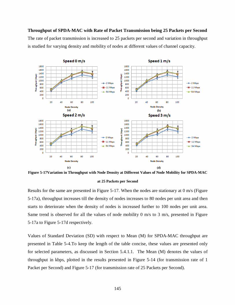
145


The rate of packet transmission is increased to 25 packets per second and variation in throughput

is studied for varying density and mobility of nodes at different values of channel capacity.

Figure 5-17Variation in Throughput with Node Density at Different Values of Node Mobility for SPDA-MAC


Results for the same are presented in Figure 5-17. When the nodes are stationary at 0 m/s (Figure

5-17a), throughput increases till the density of nodes increases to 80 nodes per unit area and then

starts to deteriorate when the density of nodes is increased further to 100 nodes per unit area.

Same trend is observed for all the values of node mobility 0 m/s to 3 m/s, presented in Figure

5-17a to Figure 5-17d respectively.

Values of Standard Deviation (SD) with respect to Mean (M) for SPDA-MAC throughput are

presented in Table 5-4.To keep the length of the table concise, these values are presented only

for selected parameters, as discussed in Section 5.4.1.1. The Mean (M) denotes the values of

throughput in kbps, plotted in the results presented in Figure 5-14 (for transmission rate of 1

Packet per Second) and Figure 5-17 (for transmission rate of 25 Packets per Second).

(a) (b)

(c) (d)

146

Table 5-4 Standard Deviation with respect to Mean for SPDA-MAC Throughput

SPDA-MAC Throughput 1 Packet per Second


0 m/s 3 m/s 0 m/s 3 m/s 0 m/s 3 m/s


20 33 0.8 31.7 0.9 34.3 1 33.5 1 34 1 33 1

60 99 0.9 93.5 1.2 100 1 97.3 1.8 106 1 93.8 1.7

100 173 5.2 173 6.9 178 5 173 5 178 5 175 5

SPDA-MAC Throughput 25 Packet per Second


0 m/s 3 m/s 0 m/s 3 m/s 0 m/s 3 m/s


20 440 52 434 45 508 59 505 55 516 61 510 57

60 1137 62 1047 82 1311 78.6 1216 101 1331 85 1247 111

100 1224 93 1216 100 1372 148 1367 138 1395 155 1372 144

Following inferences can be drawn from the results presented in Figure 5-14 to Figure 5-17, and

Table 5-4

1. With the rate of transmission of packets being 1 and 5 packets per second, throughput

achieved by SPDA-MAC is same as that of DPDA-MAC. This is because at lower rates of

transmission of packets (1 and 5 packets per second) SPDA-MAC is as capable as DPDA-

MAC to transmit the packets. However, difference in the performance of SPDA-MAC and

DPDA-MAC is visible when rate of packet transmission is increased to 15 and 25 packets

per second. At packet transmission rates of 15 and 25 packets per second, throughput

achieved with SPDA-MAC is lesser than that achieved with DPDA-MAC

2. With SPDA-MAC, throughput achieved with the rate of packet transmission being 15

packets per second is same as that achieved with 25 packets per second. It is to be noted

that the number of packets required to be transmitted are the ones that application layer

asks the node to transmit. However, there is a maximum limit for the number of packets

that channel can carry at a given time. Increasing the number of packets to be transmitted

beyond this limit does not make any difference to throughput because the capacity of the

147

channel has already been reached. SPDA-MAC uses single polarisation channel for

communication. The capacity of channel reaches its limit with packet transmission rate of

15 packets per second. Therefore, when the rate of packet transmission is increased to 25

packets per second, no further increase in throughput is observed

3. At low rates of packet transmission (1 and 5 packets per second), performance with channel

capacity of 2 Mbps is as good as 11 Mbps and 54 Mbps. This is because at lower rates of

packet transmission, channel with capacity of 2 Mbps is able to handle the traffic as well as

the channel with capacity of 54 Mbps. However, when the rate of packet transmission is

increased to 15 and 25 packets per second, it is observed that the throughput achieved with

channel capacity of 2 Mbps is lesser than that achieved with channel capacity of 11 Mbps

and 54 Mbps

4. At packet transmission rates of 1 and 5 packets per second, throughput consistently increases

with increase in density of nodes. This is because as the density of nodes increases, number

of transmitters and receivers also increases leading to increase in the number of packets

exchanged over the network. This leads to increase in throughput with increase in density

of nodes in the network. When the rate of packet transmission is increased to 15 and 25

packets per second, throughput increases up to the node density of 80 nodes per unit area,

and then deteriorates when density of nodes is further increased to 100 nodes per unit area.

This is because after certain value of node density (80 nodes per unit area in this case),

network congestion and contention between nodes to access the medium increases, leading

to deterioration of throughput

5. Node mobility does not affect the performance of SPDA-MAC drastically. This is because

the nodes in the simulated MANET scenario move at speeds of 0 m/s (stationary nodes) to

3 m/s, with a pause time of 4s to simulate walking and running speeds of humans. At these

speeds, it is observed that the performance of simulated MANET using SPDA-MAC does

not get affected drastically

148

6. From the values of standard deviation presented in Table 5-4 it is seen that standard

deviation increases with increase in traffic load on the network. This trend is same as that

observed with DPDA-MAC and it is discussed in detail in Section 5.4.1.1.

5.4.1.3 Analysis of the Variation in Throughput of CSMA/CA

This section presents study and analysis of variation in throughput when CSMA/CA is used to

access the medium and communicate with next hop node. CSMA/CA is IEEE 802.11 based

MAC protocol which carries out omnidirectional communication over single polarisation. This

study is also carried out with varying density and mobility of nodes at different values of channel

capacity.

The rates of packet transmission used for this study are 1, 5, 15 and 25 packets per second, for

which results are presented in Figure 5-18, Figure 5-19, Figure 5-20 and Figure 5-21

respectively.

Throughput of CSMA/CA with Rate of Packet Transmission being 1 Packet per Second

Throughput of CSMA/CA with packet transmission rate 1 packet per second is presented in

Figure 5-18. When nodes move at 3 m/s (Figure 5-18 d), for channel capacity of 2 Mbps,

throughput with 20 nodes per unit area is 17 kbps and that with 100 nodes per unit area is 93.7

kbps.

For the same value of node mobility, when capacity of the channel is increased to 54 Mbps,

throughput is 21.3 kbps for 20 nodes per unit area and 95 kbps for 100 nodes per unit area.

Throughput obtained with channel capacity of 2 Mbps is lower than that obtained with 54 Mbps.

It is observed that node mobility does not affect the throughput drastically.

149

Figure 5-18Variation in Throughput with Node Density at Different Values of Node Mobility for CSMA/CA

at 1 Packet per Second

Throughput of CSMA/CA with Rate of Packet Transmission being 5 Packets per Second

The rate of packet transmission is increased to 5 packets per second and results for variation in

throughput are presented in Figure 5-19. It is observed that overall throughput increases with

increase in the rate of packet transmission and with increase in node density.

Throughput obtained with channel capacity of 2 Mbps is much lower than that obtained with

channel capacity of 54 Mbps. This is expected because with increase in the rate of packet

transmission more packets are transmitted in the medium leading to increase in throughput of the

network.

(b) (a)

(c) (d)

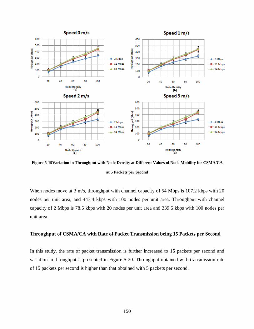
150



When nodes move at 3 m/s, throughput with channel capacity of 54 Mbps is 107.2 kbps with 20

nodes per unit area, and 447.4 kbps with 100 nodes per unit area. Throughput with channel

capacity of 2 Mbps is 78.5 kbps with 20 nodes per unit area and 339.5 kbps with 100 nodes per

unit area.


In this study, the rate of packet transmission is further increased to 15 packets per second and

variation in throughput is presented in Figure 5-20. Throughput obtained with transmission rate

of 15 packets per second is higher than that obtained with 5 packets per second.

(b) (a)

(c) (d)

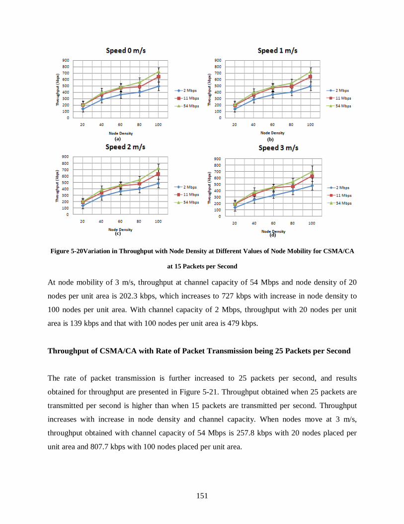
151



At node mobility of 3 m/s, throughput at channel capacity of 54 Mbps and node density of 20

nodes per unit area is 202.3 kbps, which increases to 727 kbps with increase in node density to

100 nodes per unit area. With channel capacity of 2 Mbps, throughput with 20 nodes per unit

area is 139 kbps and that with 100 nodes per unit area is 479 kbps.


The rate of packet transmission is further increased to 25 packets per second, and results

obtained for throughput are presented in Figure 5-21. Throughput obtained when 25 packets are

transmitted per second is higher than when 15 packets are transmitted per second. Throughput

increases with increase in node density and channel capacity. When nodes move at 3 m/s,

throughput obtained with channel capacity of 54 Mbps is 257.8 kbps with 20 nodes placed per

unit area and 807.7 kbps with 100 nodes placed per unit area.

(a) (b)

(c) (d)

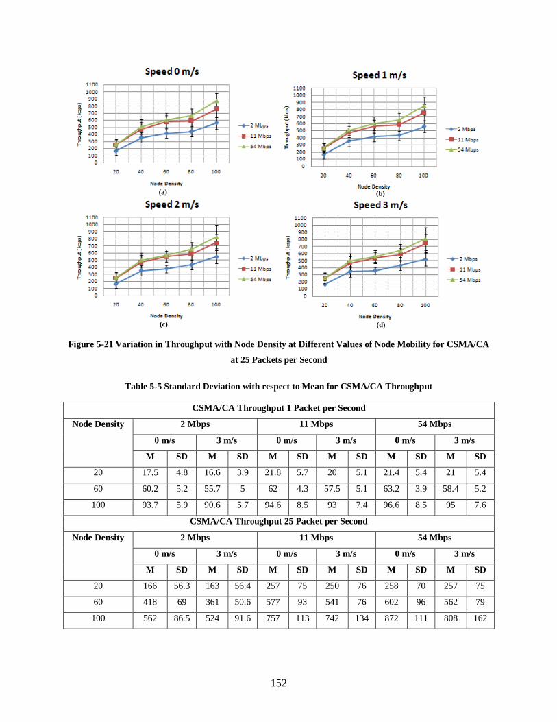
152

Figure 5-21 Variation in Throughput with Node Density at Different Values of Node Mobility for CSMA/CA


Table 5-5 Standard Deviation with respect to Mean for CSMA/CA Throughput

CSMA/CA Throughput 1 Packet per Second


0 m/s 3 m/s 0 m/s 3 m/s 0 m/s 3 m/s


20 17.5 4.8 16.6 3.9 21.8 5.7 20 5.1 21.4 5.4 21 5.4

60 60.2 5.2 55.7 5 62 4.3 57.5 5.1 63.2 3.9 58.4 5.2

100 93.7 5.9 90.6 5.7 94.6 8.5 93 7.4 96.6 8.5 95 7.6

CSMA/CA Throughput 25 Packet per Second


0 m/s 3 m/s 0 m/s 3 m/s 0 m/s 3 m/s


20 166 56.3 163 56.4 257 75 250 76 258 70 257 75

60 418 69 361 50.6 577 93 541 76 602 96 562 79

100 562 86.5 524 91.6 757 113 742 134 872 111 808 162

(a) (b)

(c) (d)

153

Values of Standard Deviation (SD) with respect to Mean (M) for CSMA/CA throughput are



throughput in kbps, plotted in the results presented in Figure 5-18 (for transmission rate of 1


From the results for network throughput achieved by CSMA/CA for different rates of packet

transmission presented in Figure 5-18 to Figure 5-21, following inferences can be made

1. Network throughput increases with increase in node density. This is expected because

increase in density of nodes leads to increase in the number of transmitters and receivers

which further increases the number of packets exchanged in the network. This leads to

increase in the throughput of the network when density of nodes is increased

2. Network throughput increases with increase in rate of packet transmission. Increase in the

rate of packet transmission leads to more packets present in the channel at a given time.

This leads to increase in network throughput

3. At the packet transmission rate of 1 packet per second, throughput achieved with channel

capacity of 2Mbps is almost same as that achieved with 11 Mbps and 54 Mbps. This is

because at the rate of 1 packet per second channel capacity of 2 Mbps is as sufficient as

channel capacity of 11 Mbps and 54 Mbps to carry data packets. However, at higher rates

of packet transmission (5, 15 and 25 packets per second), difference in throughput due to

capacity of channel becomes visible. With packet transmission rates of 5, 15 and 25

packets per second it is observed that the throughput achieved with channel capacity of 2

Mbps is lesser than that achieved with channel capacities of 11 Mbps and 54 Mbps

4. It is observed that throughput does not get affected drastically with variation in node

mobility from 0 m/s (stationary nodes) to 3 m/s and pause time of 4s

154

5. From the values of standard deviation presented in Table 5-5, it is seen that standard

deviation increases with increase in traffic load on the network. This trend is same as that

observed with DPDA-MAC and it is discussed in detail in Section 5.4.1.1.

5.4.2 Effect of Variation in Density and Mobility of Nodes on Per-Hop Delay

Achieved by DPDA-MAC, SPDA-MAC and CSMA/CA with Varying Rate of Packet

Transmission

This section studies and compares the performance of DPDA-MAC, SPDA-MAC and

CSMA/CA in terms of per-hop delay. Per-hop delay is an essential parameter to present the

performance of a MAC protocol. It is measured as the difference in time when a packet is ready

to be transmitted, till it reaches the receiver. Density and mobility of nodes, available capacity of

channel, rate of packet transmission and use of DPDA-MAC, SPDA-MAC or CSMA/CA can

affect the per-hop delay. This parameter can get affected with availability or unavailability of the

medium to be accessed by the nodes for packet transmission when density of nodes, capacity of

channel and rate of packet transmission is varied. Like the study of variation in throughput, for

this study of variation in per-hop delay also, the rate of packet transmission is varied as 1, 5, 15

and 25 packets per second. Values of channel capacity considered for this study are 2 Mbps, 11

Mbps and 54 Mbps. Density of nodes is varied from 20 to 100 nodes per unit area in steps of 20.

Mobility of nodes is varied from 0 m/s (stationary nodes) to 3 m/s, in steps of 1 m/s.

5.4.2.1 Analysis of Variation in Per-Hop Delay of DPDA-MAC

The DPDA-MAC protocol uses orthogonal polarisations for data communication. Periodic

broadcasts are exchanged among the nodes every 1000 ms to update NT. Apart from that, nodes

also broadcast Link ID information after connection establishment (after exchange of RTS-CTS

frames) and successful data transmission (after exchange of Data-ACK frames). These

intermediate broadcasts help in getting information about available or busy polarisation at

neighbour nodes, deafness avoidance, node location information for antenna beamforming and

optional power control and to update NT.

Due to the unique characteristic of DPDA-MAC of carrying out dual polarised directional

communication and broadcast of Link ID information, it becomes essential to study the variation

155

in its performance in terms of per-hop delay with varying density and mobility of nodes, rate of

packet transmission and capacity of channel.

Per-Hop Delay of DPDA-MAC with Rate of Packet Transmission being 1 Packet per

Second

Time taken for transmission of packets from one node to its next hop neighbour (per-hop delay)

is measured for varying density and mobility of nodes, when rate of packet transmission is 1

packet per second. The results for the same are presented in Figure 5-22.

Figure 5-22 Variation in Per-Hop Delay with Node Density at Different Values of Node Mobility for DPDA-

MAC at 1 Packet per Second

When node mobility is 0 m/s (Figure 5-22 a), per-hop delay at 54 Mbps with 20 nodes per unit

area is 60.1 ms, and that with 100 nodes per unit area is 142.4 ms. When node mobility is

increased to 3 m/s (Figure 5-22 d), per-hop delay with 20 nodes per unit area is 60.9 ms and with

100 nodes per unit area it is 145.7 ms. At channel capacity of 2 Mbps and nodes are stationary

(Figure 5-22 a), per-hop delay with 20 nodes per unit area is 77.5 ms and that with 100 nodes per

(a) (b)

(c) (d)

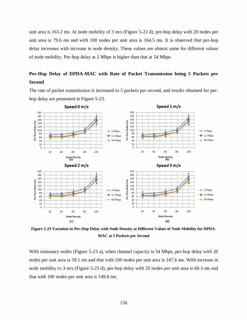
156

unit area is 163.2 ms. At node mobility of 3 m/s (Figure 5-22 d), per-hop delay with 20 nodes per

unit area is 79.6 ms and with 100 nodes per unit area is 164.5 ms. It is observed that per-hop

delay increases with increase in node density. These values are almost same for different values

of node mobility. Per-hop delay at 2 Mbps is higher than that at 54 Mbps.

Per-Hop Delay of DPDA-MAC with Rate of Packet Transmission being 5 Packets per

Second

The rate of packet transmission is increased to 5 packets per second, and results obtained for per-

hop delay are presented in Figure 5-23.



With stationary nodes (Figure 5-23 a), when channel capacity is 54 Mbps, per-hop delay with 20

nodes per unit area is 59.1 ms and that with 100 nodes per unit area is 147.6 ms. With increase in

node mobility to 3 m/s (Figure 5-23 d), per-hop delay with 20 nodes per unit area is 60.3 ms and

that with 100 nodes per unit area is 149.8 ms.

(a) (b)

(c) (d)

157

When capacity of the channel is reduced to 2 Mbps, per-hop delay for stationary nodes (Figure

5-23a) with node density of 20 nodes per unit area is 72.3 ms and that with 100 nodes per unit

area is 170.3 ms. When mobility of nodes is 3 m/s (Figure 5-23d), per-hop delay with 20 nodes

per unit area is 74.4 ms and that with 100 nodes per unit area is 170.8 ms.


Second

The rate of packet transmission is increased to 15 packets per second and results for per-hop

delay are presented in Figure 5-24.



From the obtained results it is observed that per-hop delay increases with increase in node

density and reduction in channel capacity. Slight increase in per-hop delay is observed with

increase in node mobility. At the channel capacity of 54 Mbps, when nodes are stationary

(Figure 5-24a), per-hop delay with 20 nodes per unit area is 59.4 ms and with 100 nodes per unit

area it is 152.1 ms. For node mobility of 3 m/s (Figure 5-24 d), per-hop delay with 20 nodes per

unit area is 59.6 ms and that with 100 nodes per unit area is 153.1 ms. When channel capacity is

(a) (b)

(c) (d)

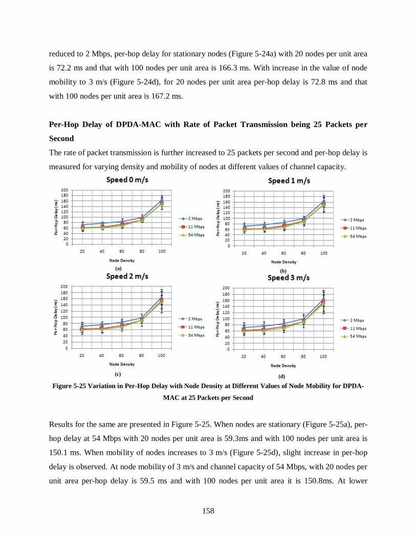
158

reduced to 2 Mbps, per-hop delay for stationary nodes (Figure 5-24a) with 20 nodes per unit area

is 72.2 ms and that with 100 nodes per unit area is 166.3 ms. With increase in the value of node

mobility to 3 m/s (Figure 5-24d), for 20 nodes per unit area per-hop delay is 72.8 ms and that

with 100 nodes per unit area is 167.2 ms.


Second

The rate of packet transmission is further increased to 25 packets per second and per-hop delay is

measured for varying density and mobility of nodes at different values of channel capacity.



Results for the same are presented in Figure 5-25. When nodes are stationary (Figure 5-25a), per-

hop delay at 54 Mbps with 20 nodes per unit area is 59.3ms and with 100 nodes per unit area is

150.1 ms. When mobility of nodes increases to 3 m/s (Figure 5-25d), slight increase in per-hop

delay is observed. At node mobility of 3 m/s and channel capacity of 54 Mbps, with 20 nodes per

unit area per-hop delay is 59.5 ms and with 100 nodes per unit area it is 150.8ms. At lower

(a) (b)

(c) (d)

159

channel capacities of 2 Mbps, when nodes are stationary (Figure 5-25a) and density of nodes is

20 nodes per unit area, value of per-hop delay is 71.3 ms and it increase to 163.3ms when density

of nodes increases to 100 nodes per unit area. When mobility of nodes increases to 3 m/s keeping

channel capacity as 2 Mbps, with 20 nodes per unit area the value of per-hop delay is 71.6 ms

and it increases to 163.6 ms when density of nodes increases to 100 nodes per unit area.

Table 5-6 Standard Deviation with respect to Mean for DPDA-MAC Per-Hop Delay

DPDA-MAC Per-Hop Delay 1 Packet per Second


0 m/s 3 m/s 0 m/s 3 m/s 0 m/s 3 m/s


20 77.5 11 79.6 14.3 64.8 10 66 9.8 60.1 6.1 61 9

60 88.4 7.9 88.9 9.9 75.6 6.6 77 7.4 69 6 70 6.5

100 163 17.4 165 18 150 21 151 19.2 142 17 146 18

DPDA-MAC Per-Hop Delay 25 Packet per Second


0 m/s 3 m/s 0 m/s 3 m/s 0 m/s 3 m/s


20 71.3 11.7 71.6 15.9 62 10.5 62.4 16.7 59.3 9.5 60 9.2

60 84.6 11 84.7 14.2 73.7 9.6 74 17.6 68.8 8.2 69 6.1

100 163 17.6 164 23.7 151 22.7 154 37.8 150 21 151 26

Values of Standard Deviation (SD) with respect to Mean (M) for DPDA-MAC Per-Hop Delay

are presented in Table 5-6.To keep the length of the table concise, these values are presented

only for selected parameters, as discussed in Section 5.4.1.1. The Mean (M) denotes the values

of per-hop delay in ms, plotted in the results presented in Figure 5-22 (for transmission rate of 1


From the results depicted in Figure 5-22 to Figure 5-25, and Table 5-6 following inferences can

be drawn

1. Per-hop delay increases with increase in node density. This is because, with increase in

node density, number of nodes trying to access the medium increases. This gives rise to

increased contention periods among the nodes, leading to increased per-hop delays

160

2. Per-hop delay for different rates of packet transmission for a given node density is almost

same, provided the capacity of the channel remains same. It is measured as the difference

in time when a packet is ready to be transmitted, till it reaches the next hop node. For a

given MAC protocol (DPDA-MAC) this time remains almost constant for different rates

of packet transmission as only one hop communication is considered here

3. The experienced per-hop delay does not change drastically with variation in mobility of

nodes. The variation in mobility of nodes from 0 m/s to 3 m/s with pause time of 4s

which simulates walking and running speed of humans does not affect the performance of

the protocol drastically

4. When capacity of the channel is reduced, value of per-hop delay increases. This is

expected because lesser the capacity of the channel lesser is its capability to carry

information, leading to higher delays

5. From Table 5-6, it is seen that standard deviation increases with increase in node density

because at higher node density, more nodes try to access the medium and may find

medium busy, leading to random backoff delays. This leads to variation in per-hop delay

for packets exchanged between different communicating nodes. More instances of

random backoff delays cause the per-hop delay across different seeds to vary. In some

cases the absolute value of the standard deviation at higher node densities is lesser than at

lower densities. However, when it is expressed as a percentage of its corresponding

mean, the standard deviation with respect to mean is more.

5.4.2.2 Analysis of Variation in Per-Hop Delay of SPDA-MAC

SPDA-MAC protocol uses single polarisation for directional communication. However,

directional communication leads to the problem of deafness. Therefore, like DPDA-MAC,

SPDA-MAC also broadcasts Link ID information periodically for updating NT and avoidance of

deafness. With additional packets exchanged for broadcast of Link ID information, per-hop delay

becomes an essential parameter to determine the performance SPDA-MAC. The variation in per-

161

hop delay with varying node density, mobility and channel capacity for transmission rates of 1,

5, 15 and 25 packets per second is presented in Figure 5-26 to Figure 5-29.

Per-Hop Delay of SPDA-MAC with Rate of Packet Transmission being 1 Packet per

Second

The per-hop delay obtained when SPDA-MAC is used for communication with next hop node at

packet transmission rate of 1 packet per second is presented in Figure 5-26.

Figure 5-26Variation in Per-Hop Delay with Node Density at Different Values of Node Mobility for SPDA-

MAC at 1 Packet per Second

With channel capacity of 54 Mbps, when nodes move at 3 m/s (Figure 5-26 d), per-hop delay

with 20 nodes per unit area is 64.9 ms and with 100 nodes per unit area is 137.6 ms. At channel

capacity of 2 Mbps, per-hop delay with 20 nodes per unit area is 80.8 ms and with 100 nodes per

unit area is 151 ms. From the obtained results it can be observed that per-hop delay increases

with increase in node density and reduction in capacity of the channel. Increase in node mobility

leads to slight increase in per-hop delay.

(a) (b)

(c) (d)

162

Per-Hop Delay of SPDA-MAC with Rate of Packet Transmission being 5 Packets per

Second

Per-hop delay for SPDA-MAC when rate of packet transmission is increased to 5 packets per

second is presented Figure 5-27.



With nodes moving at 3 m/s (Figure 5-27d), and channel capacity being 54 Mbps, per-hop delay

with 20 nodes per unit area is 64.1 ms and it increases to 137.5 ms when density of nodes is

increased to 100 nodes per unit area.

When channel capacity is reduced to 2 Mbps with node mobility of 3 m/s, per-hop delay with 20

nodes per unit area is 75.9ms and it increases to 153.2ms when density of nodes is increased to

100 nodes per unit area.

(a) (b)

(c) (d)

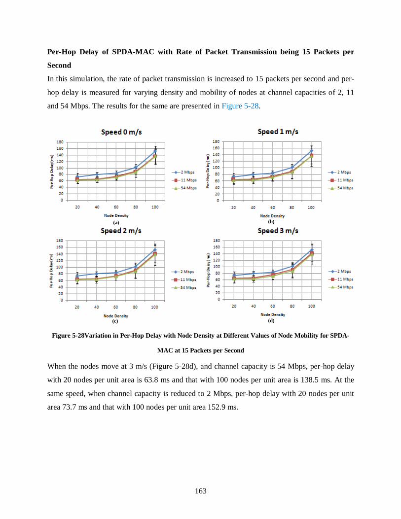
163


Second

In this simulation, the rate of packet transmission is increased to 15 packets per second and per-

hop delay is measured for varying density and mobility of nodes at channel capacities of 2, 11

and 54 Mbps. The results for the same are presented in Figure 5-28.



When the nodes move at 3 m/s (Figure 5-28d), and channel capacity is 54 Mbps, per-hop delay

with 20 nodes per unit area is 63.8 ms and that with 100 nodes per unit area is 138.5 ms. At the

same speed, when channel capacity is reduced to 2 Mbps, per-hop delay with 20 nodes per unit

area 73.7 ms and that with 100 nodes per unit area 152.9 ms.

(a) (b)

(d) (c)

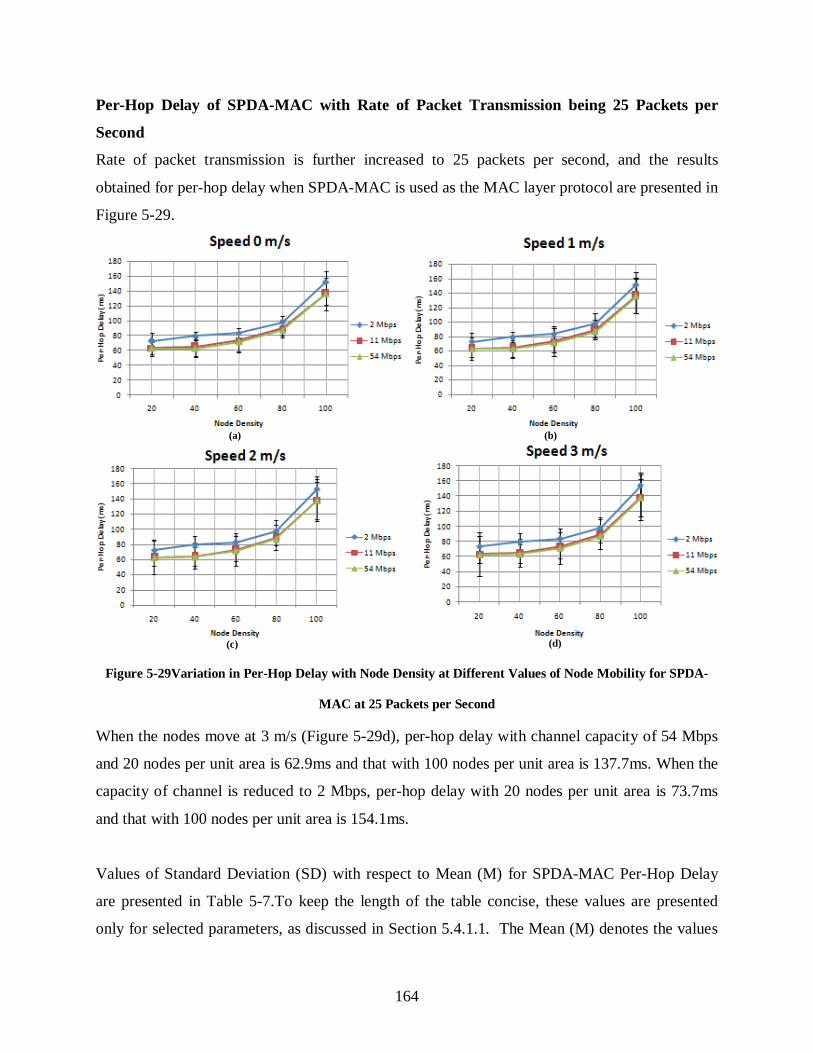
164


Second

Rate of packet transmission is further increased to 25 packets per second, and the results

obtained for per-hop delay when SPDA-MAC is used as the MAC layer protocol are presented in

Figure 5-29.



When the nodes move at 3 m/s (Figure 5-29d), per-hop delay with channel capacity of 54 Mbps

and 20 nodes per unit area is 62.9ms and that with 100 nodes per unit area is 137.7ms. When the

capacity of channel is reduced to 2 Mbps, per-hop delay with 20 nodes per unit area is 73.7ms

and that with 100 nodes per unit area is 154.1ms.

Values of Standard Deviation (SD) with respect to Mean (M) for SPDA-MAC Per-Hop Delay

are presented in Table 5-7.To keep the length of the table concise, these values are presented

only for selected parameters, as discussed in Section 5.4.1.1. The Mean (M) denotes the values

(a) (b)

(c) (d)

165

of per-hop delay in ms, plotted in the results presented in Figure 5-26 (for transmission rate of 1


Table 5-7 Standard Deviation with respect to Mean for SPDA-MAC Per-Hop Delay

SPDA-MAC Per-Hop Delay 1 Packet per Second


0 m/s 3 m/s 0 m/s 3 m/s 0 m/s 3 m/s


20 80.3 12.4 80.8 12.5 64.8 10.2 68.3 10.8 63.2 10.5 65 11.4

60 84.6 7.8 86.6 8 75.3 9.2 76 7 71 8 71.2 6.7

100 150.2 13.8 151 13.9 137.7 15.1 138 17 137.4 16.4 137 16.2

SPDA-MAC Per-Hop Delay 25 Packet per Second


0 m/s 3 m/s 0 m/s 3 m/s 0 m/s 3 m/s


20 72.8 11.4 73.7 13 63.4 11.4 63.5 28.5 62.7 8.1 62.9 11.3

60 83.3 6.6 84 8.3 73.3 16 73.5 23.1 71.3 12.7 71.9 13.5

100 152 14.7 154 17 136.8 15 138.6 30.4 136 21.6 138 24.6

From the results presented in Figure 5-26 to Figure 5-29, and Table 5-7, following inferences can

be drawn

1. Per-hop delay increases with increase in node density. With increased density of nodes,

the number of transmitters trying to access the network also increases. This increases the

contention among nodes to access the medium

2. Value of per-hop delay at different rates of packet transmission is almost same. This is

because, to study the performance of SPDA-MAC, the delay value is calculated only over

one hop. Provided the capacity of the channel is kept same, time taken for a packet to

travel from one node to its next hop remains same regardless of changein the rate of

packet transmission

166

3. Node mobility introduces only slight increase in per-hop delay. Nodes are simulated to

move according to walking and running speed of humans. The value of node mobility is

varied from 0 m/s to 3 m/s with a pause time of 4s. It is observed that at these values of

node mobility performance of the network does not get affected drastically

4. Reducing channel capacity increases per-hop delay. This is expected because capacity of

a channel denotes channel’s ability to carry certain amount of information at a given

time. When capacity of the channel is reduced, the its ability to carry information also

reduces, leading to increase in time taken to carry information from one node to another

5. From the values of standard deviation presented in Table 5-7 it is seen that standard

deviation increases with increase in node density. This trend is same as that observed

with DPDA-MAC and it is discussed in detail in Section 5.4.2.1.

5.4.2.3 Analysis of Variation in Per-Hop Delay of CSMA/CA

CSMA/CA is the IEEE 802.11 based method for medium access control in wireless networks. In

this method, nodes communicate omnidirectionally in Vertical Polarisation (VP).

Omnidirectional communication brings in certain disadvantages such as higher instances of

exposed node problem and increased interference. However, nodes do not experience deafness

with omnidirectional communication. Therefore, with omnidirectional communication in single

polarisation of CSMA/CA, broadcast of Link ID information is not needed at any instance.

Since Link ID information is not broadcasted after exchange of RTS-CTS and Data-ACK

frames, the per-hop delay obtained with CSMA/CA is different from that obtained with DPDA-

MAC and SPDA-MAC protocols. In this section, per-hop delay when CSMA/CA is used as the

MAC layer protocol is presented for varying density and mobility of nodes. The channels with 2,

11 and 54 Mbps capacity are considered for this study. Rates of packet transmission considered

for this study are 1, 5, 15 and 25 packets per second. Results for the same are presented in Figure

5-30 to Figure 5-33.

167

Per-Hop Delay of CSMA/CA with Rate of Packet Transmission being 1 Packet per Second

The results obtained for per-hop delay when CSMA/CA is used as the MAC layer and rate of

packet transmission is 1 packet per second, are presented in Figure 5-30. From the obtained

results it is observed that per-hop delay increases marginally with increase in density of nodes.

Figure 5-30 Variation in Per-Hop Delay with Node Density at Different Values of Node Mobility for

CSMA/CA at 1 Packet per Second

The per-hop delay obtained with channel capacity of 2 Mbps is higher than that obtained with

channel capacity of 54 Mbps. Slight increase in per-hop delay is observed with increase in

mobility of nodes. When the nodes move at 3 m/s (Figure 5-30 d), and capacity of channel is 54

Mbps, per-hop delay with 20 nodes per unit area is 41.6 ms and that with 100 nodes per unit area

is 48.6 ms. With same node mobility, when capacity of channel is reduced to 2 Mbps, per-hop

delay obtained with 20 nodes per unit area is 53.4ms and that with 100 nodes per unit area is

67.7 ms.

(a) (b)

(c) (d)

168

Per-Hop Delay of CSMA/CA with Rate of Packet Transmission being 5 Packets per Second

The rate of transmission is increased to 5 packets per second and results for per-hop delay are

obtained for different values of density and mobility of nodes with varying channel capacity. The

results for the same are presented in Figure 5-31.


CSMA/CA at 5 Packets per Second

When the nodes move at 3 m/s (Figure 5-31d), per-hop delay with channel capacity of 54 Mbps

and node density of 20 nodes per unit area is 42.8 ms and that with 100 nodes per unit area is

48.9 ms.

At same node mobility, when capacity of the channel is reduced to 2 Mbps, per-hop delay with

20 nodes per unit area is 55 ms and that with 100 nodes per unit area is 69 ms. Therefore, it is

observed that per-hop delay increases with increase in node density and reduction in channel

capacity.

(a) (b)

(c) (d)

169

Per-Hop Delay of CSMA/CA with Rate of Packet Transmission being 15 Packets per

Second

The rate of packet transmission is increased to 15 packets per second and results obtained for

per-hop delay when CSMA/CA is used for medium access control are presented in Figure 5-32.



When nodes move at 3 m/s (Figure 5-32d), value of per-hop delay with channel capacity of 54

Mbps and node density of 20 nodes per unit area is 45 ms and that with 100 nodes per unit area

is 50.1 ms. When channel capacity is reduced to 2 Mbps, keeping value of node mobility same,

per-hop delay with 20 nodes per unit area is 56.5 Mbps and that with 100 nodes per unit area

72.8 ms. Therefore, from the obtained results it is observed that per-hop delay with packet

transmission rate of 15 packets per second is higher than that with 5 packets per second. It

increases with increase in node density and reduction in channel capacity. Increase in node

mobility induces marginal increase in per-hop delay for all values in node density and channel

capacities.

(a) (b)

(c) (d)

170

Per-Hop Delay of CSMA/CA with Rate of Packet Transmission being 25 Packets per

Second

In this study, rate of packet transmission is further increased to 25 packets per second and the

results for the same are presented in Figure 5-33.



With nodes moving at 3 m/s (Figure 5-33 d), when capacity of the channel is 54 Mbps and

density of nodes in 20 nodes per unit area, the per-hop delay obtained is 55.5 ms and that with

100 nodes per unit area is 59 ms. At same values of node mobility, when channel capacity of

reduced to 2 Mbps, per-hop delay with 20 nodes per unit area 67.4 ms and that with 100 nodes

per unit area is 80.6 ms. Therefore, it is observed that per-hop delay when 25 packets are

transmitted per second is higher than that obtained when 15 packets are transmitted per second. It

is also observed that per-hop delay increases with increase in node density and reduction in

channel capacity.

(a) (b)

(d) (c)

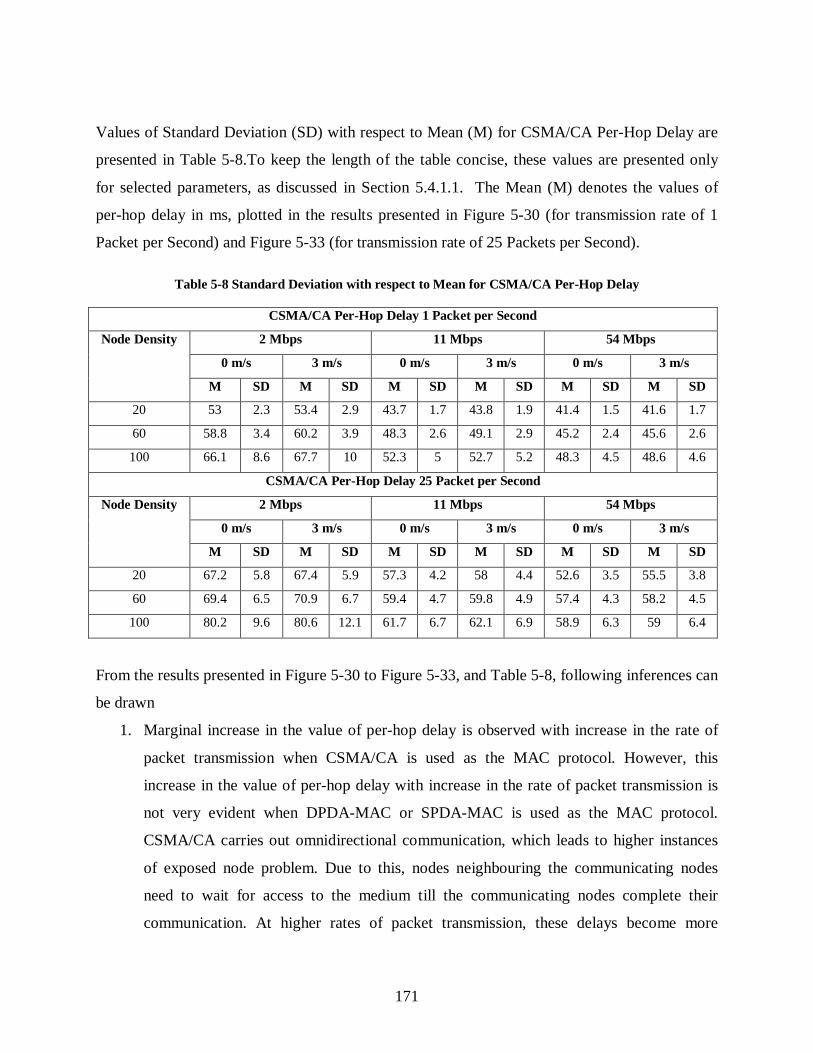
171

Values of Standard Deviation (SD) with respect to Mean (M) for CSMA/CA Per-Hop Delay are



per-hop delay in ms, plotted in the results presented in Figure 5-30 (for transmission rate of 1


Table 5-8 Standard Deviation with respect to Mean for CSMA/CA Per-Hop Delay

CSMA/CA Per-Hop Delay 1 Packet per Second


0 m/s 3 m/s 0 m/s 3 m/s 0 m/s 3 m/s


20 53 2.3 53.4 2.9 43.7 1.7 43.8 1.9 41.4 1.5 41.6 1.7

60 58.8 3.4 60.2 3.9 48.3 2.6 49.1 2.9 45.2 2.4 45.6 2.6

100 66.1 8.6 67.7 10 52.3 5 52.7 5.2 48.3 4.5 48.6 4.6

CSMA/CA Per-Hop Delay 25 Packet per Second


0 m/s 3 m/s 0 m/s 3 m/s 0 m/s 3 m/s


20 67.2 5.8 67.4 5.9 57.3 4.2 58 4.4 52.6 3.5 55.5 3.8

60 69.4 6.5 70.9 6.7 59.4 4.7 59.8 4.9 57.4 4.3 58.2 4.5

100 80.2 9.6 80.6 12.1 61.7 6.7 62.1 6.9 58.9 6.3 59 6.4

From the results presented in Figure 5-30 to Figure 5-33, and Table 5-8, following inferences can

be drawn

1. Marginal increase in the value of per-hop delay is observed with increase in the rate of

packet transmission when CSMA/CA is used as the MAC protocol. However, this

increase in the value of per-hop delay with increase in the rate of packet transmission is

not very evident when DPDA-MAC or SPDA-MAC is used as the MAC protocol.

CSMA/CA carries out omnidirectional communication, which leads to higher instances

of exposed node problem. Due to this, nodes neighbouring the communicating nodes

need to wait for access to the medium till the communicating nodes complete their

communication. At higher rates of packet transmission, these delays become more

172

evident. In case of DPDA-MAC and SPDA-MAC instances of nodes undergoing the

problem of exposed nodes is lesser when compared to CSMA/CA. In DPDA-MAC

instances of nodes undergoing the problem of directional exposed nodes also reduces.

Therefore, variation in per-hop delay with variation in the rate of packet transmission is

not evident with DPDA-MAC or SPDA-MAC when compared to CSMA/CA

2. The value of per-hop delay is observed to increase with increase in node density. This is

mainly because of the increase in network contention due to the increase in number of

transmitters

3. Per-hop delay does not increase with increase in node mobility. This is mainly because

the simulated values of node mobility (walking and running speed of humans) do not

affect the performance of the network drastically. Also, values for only one hop

transmission are considered for this study, which does not get drastically affected due to

node mobility as nodes may not go out of communication range

4. The value of per-hop delay increases with reduction of channel capacity. This is expected

because reducing the capacity of the channel reduces its ability to carry information at a

given time, leading to increase in per-hop delay

5. From the values of standard deviation presented in Table 5-8, it is seen that standard

deviation increases with increase in node density. This trend is same as that observed

with DPDA-MAC and it is discussed in detail in Section 5.4.2.1.

5.4.3 Comparison of Performance of DPDA-MAC, SPDA-MAC and CSMA/CA with

Node Density of 100 Nodes per Unit Area

In Sections 5.4.1 and 5.4.2, performance analysis of the three protocols namely DPDA-MAC,

SPDA-MAC and CSMA/CA was presented, in terms of throughput and per-hop delay. The focus

of these sections was on the individual performance of the three protocols. This section presents

the comparison of throughput of three MAC protocols, when the node density is 100 nodes per

unit area. It is essential to study the difference in the performance of the three MAC protocols

when more nodes try to access the medium at the same time. At 100 nodes per unit area, the

173

number of nodes trying to access the medium is highest. The comparison of obtained throughput

is presented for packet transmission rates of 1, 5, 15 and 25 packets per second, channel

capacities of 54 Mbps, 11 Mbps and 2 Mbps and for node mobility values of 0 to 3 m/s increased

in steps of 1 m/s. Comparison of throughput obtained with three MAC layer protocols, with

channel capacities of 54 Mbps, 11 Mbps and 2 Mbps is presented in Figure 5-34 to Figure 5-36.

The aim of this study is to distinguish between the capabilities of the three routing protocols in

responding to the variation in rates of packet transmission.

5.4.3.1 Comparison of Throughput with Varying Packet Rate and Channel Capacity

for Node Density of 100 Nodes per Unit Area

The results comparing throughput of DPDA-MAC, SPDA-MAC and CSMA/CA are presented in

Figure 5-34a, b, c and d. The mobility of nodes is varied from 0 m/s to 3 m/s in steps of 1 m/s.

This comparison is carried out for node density of 100 nodes per unit area and channel capacity

of 54 Mbps at packet transmission rates of 1, 5, 15 and 25 packets per second.

Figure 5-34 Variation in Throughput against Node Mobility for Different Rates of Packet Transmission at 54

Mbps and 100 Nodes per Unit Area

(a) (b)

(c) (d)

174

From the results illustrated in Figure 5-34a, b, c and d, it is observed that throughput obtained

with DPDA-MAC is the highest, followed by that obtained with SPDA-MAC. Throughput

obtained with CSMA/CA is the least for all values of density and mobility of nodes.

Figure 5-35 Variation in Throughput against Node Mobility for Different Rates of Packet Transmission at

11Mbps and 100 Nodes per Unit Area

At lower transmission rates of 1 and 5 packets per second (Figure 5-34a and b), the difference

between the throughput obtained with DPDA-MAC and SPDA-MAC is very low. However, the

difference in performance of DPDA-MAC, SPDA-MAC and CSMA/CA becomes evident when

rate of packet transmission is increased to 15 packets per second (Figure 5-34 c) and 25 packets

per second (Figure 5-34d). Results for throughput obtained when capacity of the channel is

reduced to 11 Mbps are presented in Figure 5-35a, b, c and d, for different packet transmission

rates of 1, 5, 15 and 25 packets per second. These results show slight degradation in throughput

when compared to that obtained with channel capacity of 54 Mbps. With reduction in channel

capacity to 2 Mbps, further drop in throughput is observed for all the three protocols as observed

from Figure 5-36.Over all the values of channel capacities (2 Mbps, 11 Mbps and 54 Mbps), for

highest traffic load of 25 packets per second, throughput achieved with DPDA-MAC is the

highest, followed by SPDA-MAC. Throughput achieved by CSMA/CA is the least in all the

cases.

(a) (b)

(c) (d)

175



From the obtained results following observations are made

1. Throughput is least with transmission rate of 1 packet per second and highest for

transmission rate of 25 packets per second, for all the MAC protocols. This is as

expected, since increase in the rate of packet transmission increases the number of

packets exchanged over the medium for a given time, thus increasing throughput of the

network

2. Throughput reduces with reduction in channel capacity for all the three MAC protocols.

This is expected because when channel capacity is reduced, ability of the channel to carry

information reduces, leading to deterioration in throughput

3. Node mobility does not affect throughput drastically because nodes are moving at speeds

of 1, 2, and 3 m/s with a pause time 4s for all speeds. Therefore, nodes seldom go out of

(a) (b)

(c) (d)

176

range of each other. Apart from that, nodes exchange broadcast packets periodically

(every 1000 ms). With location information given in broadcast packets every 1000 ms,

transmitters can direct their beams towards the receivers

4. At packet rates of 1 packet per second and 5 packets per second, throughput of DPDA-

MAC and SPDA-MAC is almost same. However, when rate of packet transmission is

increased to 15 and 25 packets per second then DPDA-MAC performs better than SPDA-

MAC and CSMA/CA. This is because SPDA-MAC is able to handle traffic equally well

as DPDA-MAC at low packet transmission rates. However, when rate of packet

transmission is increased, throughput of DPDA-MAC is almost twice of that of SPDA-

MAC. This is because DPDA-MAC can simultaneously use orthogonal polarisations for

data transmission. SPDA-MAC uses only one polarisation for directional communication

leaving it with just one communication channel. Also, nodes can undergo directional

exposed node problem in SPDA-MAC, which is not the case with DPDA-MAC

5. Throughput of CSMA/CA is the least for all rates of packet transmission. This is mainly

because CSMA/CA carries out omnidirectional communication, due to which nodes

undergo the problem of exposed nodes leading to deterioration of performance. With use

of only one polarisation CSMA/CA is virtually left with only one channel for

communication when compared to DPDA-MAC. Therefore, use of omnidirectional

communication over single polarisation leads to low throughput of CSMA/CA when

compared to DPDA-MAC and SPDA-MAC protocols

5.4.3.2 Comparison of Per-Hop Delay with Varying Packet Rate and Channel Capacity

for Node Density of 100 Nodes per Unit Area

This section compares the per-hop delay computed when packets are transmitted from one node

to another node located one-hop away with the use of DPDA-MAC, SPDA-MAC and

CSMA/CA as MAC layer protocols.

177

Figure 5-37Variation in Per-Hop Delay against Node Mobility for Different Rates of Packet Transmission at

54 Mbps and 100 Nodes per Unit Area

Individual results for per-hop delay obtained for the three MAC layer protocols were presented

in Section 5.4.2. This section presents comparison of the per-hop delay obtained with DPDA-

MAC, SPDA-MAC and CSMA/CA for different rates of packet transmission and varying values

of mobility of nodes.

This study is carried out for node density of 100 nodes per unit area, which is the maximum

value of node density considered in this simulation. Results are presented for channel capacities

of 54 Mbps, 11 Mbps and 2 Mbps in Figure 5-37 to Figure 5-39 respectively.

The results for per-hop delay with channel capacity of 54 Mbps and node density of 100 nodes

per unit area for DPDA-MAC, SPDA-MAC and CSMA/CA are presented in Figure 5-37 for

packet transmission rates of 1, 5, 15 and 25 packets per second (Figure 5-37a, b, c and d

respectively). From the obtained results it is observed that the per-hop delay for DPDA-MAC is

highest when compared to that with SPDA-MAC and CSMA/CA.

(a) (b)

(c) (d)

178

Figure 5-38Variation in Per-Hop Delay against Node Mobility for Different Rates of Packet Transmission at

11 Mbps and 100 Nodes per Unit Area

Results for per-hop delay obtained with channel capacity of 11 Mbps for node density of 100

nodes per unit area are presented in Figure 5-38.

An increase in per-hop delay is observed with reduction in channel capacity from 54 Mbps to 11

Mbps. Results for per-hop delay obtained with channel capacity of to 2 Mbps is presented in

Figure 5-39.

Further increase in per-hop delay is observed with reduction in channel capacity to 2 Mbps.

Among all the three protocols, DPDA-MAC has the highest per-hop delay while CSMA/CA has

the least for all the values of channel capacity.

(a) (b)

(c) (d)

179

Figure 5-39Variation in Per-Hop Delay against Node Mobility for Different Rates of Packet Transmission at 2


Following inferences can be drawn from the obtained results for node density of 100 nodes per

unit area:

1. Per-hop delay for DPDA-MAC is the highest, followed by SPDA-MAC. Per-hop delay

for CSMA/CA is the least. The reason for higher per-hop delay of DPDA-MAC and

SPDA-MAC, when compared to CSMA/CA is transmission of Link ID broadcasts after

exchange of RTS-CTS frames before data packets are transmitted to the medium. In

CSMA/CA the concept of Link ID broadcast does not exist, therefore there is no

intermediate broadcast after exchange of RTS-CTS frame and before data transmission,

leading to lower values of per-hop delays when compared to DPDA-MAC and SPDA-

MAC

(a)

(c) (d)

(b)

180

2. Per-hop delay of DPDA-MAC is higher than that of SPDA-MAC. It should be noted that

all Link ID broadcasts take place in vertical polarisation, irrespective of data being

exchanged in vertical or horizontal polarisation. Link ID broadcasts are transmitted after

establishment of connection (exchange of RTS-CTS frames) and before transmission of

data packet. Therefore, even when data packet needs to be transmitted over horizontal

polarisation, it is required to wait for vertical polarisation to be available for Link ID

broadcast to take place, after which transmission of data packet can take place. This adds

to cumulative delays for transmission of packets using DPDA-MAC. In SPDA-MAC all

packets are transmitted over vertical polarisation itself. Hence, per-hop delay experienced

by transmissions with SPDA-MAC is lesser than that experienced by transmissions using

DPDA-MAC

3. Per-hop delay increases with reduction in channel capacity. This is as expected because

when capacity of the channel reduces, its ability to carry information at a given time

reduces. This leads to increase in the value of per-hop delay with reduction in channel

capacity. This trend is observed for all the three MAC protocols

4. The values of node mobility considered for this simulation (0 m/s to 3 m/s) with pause

time of 4 s do not affect the performance of the network in terms of per-hop delay

drastically. Link ID broadcasts carrying information about location of nodes are

exchanged every 1000 ms. Since per-hop delay is measured between two nodes, the

nodes moving at simulated speeds seldom go out of communication range of each other

5.4.4 Comparison of the Performance of DPDA-MAC and SPDA-MAC

Throughput is a critical parameter to analyse the performance of a protocol. The objective of this

thesis is to illustrate the importance of dual polarised directional communication to enhance the

throughput of MANETs. Therefore, this section presents the comparison of throughput obtained

by DPDA-MAC which uses dual polarised directional communication and SPDA-MAC which

carries out directional communication over single polarisation only. The variation in throughput

when DPDA-MAC and SPDA-MAC are used as the MAC layer protocols for communication

among nodes is presented in Figure 5-40.The results are presented for stationary nodes (mobility

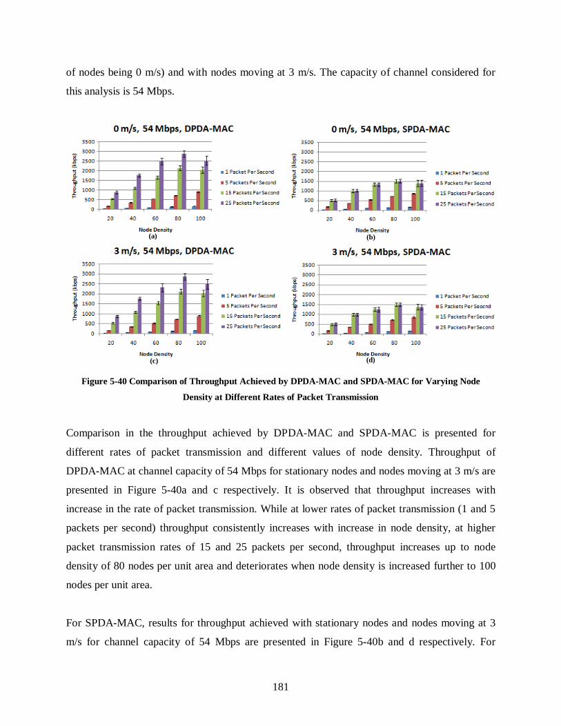
181

of nodes being 0 m/s) and with nodes moving at 3 m/s. The capacity of channel considered for

this analysis is 54 Mbps.

Figure 5-40 Comparison of Throughput Achieved by DPDA-MAC and SPDA-MAC for Varying Node

Density at Different Rates of Packet Transmission

Comparison in the throughput achieved by DPDA-MAC and SPDA-MAC is presented for

different rates of packet transmission and different values of node density. Throughput of

DPDA-MAC at channel capacity of 54 Mbps for stationary nodes and nodes moving at 3 m/s are

presented in Figure 5-40a and c respectively. It is observed that throughput increases with

increase in the rate of packet transmission. While at lower rates of packet transmission (1 and 5

packets per second) throughput consistently increases with increase in node density, at higher

packet transmission rates of 15 and 25 packets per second, throughput increases up to node

density of 80 nodes per unit area and deteriorates when node density is increased further to 100

nodes per unit area.

For SPDA-MAC, results for throughput achieved with stationary nodes and nodes moving at 3

m/s for channel capacity of 54 Mbps are presented in Figure 5-40b and d respectively. For

(a) (b)

(c) (d)

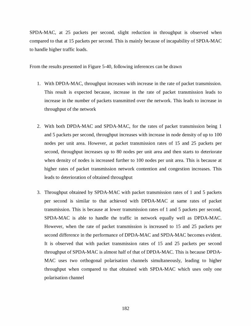
182

SPDA-MAC, at 25 packets per second, slight reduction in throughput is observed when

compared to that at 15 packets per second. This is mainly because of incapability of SPDA-MAC

to handle higher traffic loads.

From the results presented in Figure 5-40, following inferences can be drawn

1. With DPDA-MAC, throughput increases with increase in the rate of packet transmission.

This result is expected because, increase in the rate of packet transmission leads to

increase in the number of packets transmitted over the network. This leads to increase in

throughput of the network

2. With both DPDA-MAC and SPDA-MAC, for the rates of packet transmission being 1

and 5 packets per second, throughput increases with increase in node density of up to 100

nodes per unit area. However, at packet transmission rates of 15 and 25 packets per

second, throughput increases up to 80 nodes per unit area and then starts to deteriorate

when density of nodes is increased further to 100 nodes per unit area. This is because at

higher rates of packet transmission network contention and congestion increases. This

leads to deterioration of obtained throughput

3. Throughput obtained by SPDA-MAC with packet transmission rates of 1 and 5 packets

per second is similar to that achieved with DPDA-MAC at same rates of packet

transmission. This is because at lower transmission rates of 1 and 5 packets per second,

SPDA-MAC is able to handle the traffic in network equally well as DPDA-MAC.

However, when the rate of packet transmission is increased to 15 and 25 packets per

second difference in the performance of DPDA-MAC and SPDA-MAC becomes evident.

It is observed that with packet transmission rates of 15 and 25 packets per second

throughput of SPDA-MAC is almost half of that of DPDA-MAC. This is because DPDA-

MAC uses two orthogonal polarisation channels simultaneously, leading to higher

throughput when compared to that obtained with SPDA-MAC which uses only one

polarisation channel

183

4. In SPDA-MAC, throughput increases when the rate of packet transmission is increased

from 1 packet per second to 5 packets per second. However, throughput achieved with 15

packets per second is almost same as that achieved with 25 packets per second. This is

because with SPDA-MAC which uses only single polarisation for directional

communication the capacity of channel reaches its limit with packet transmission rate of

15 packets per second. Therefore, no further increase in throughput is observed when the

rate of packet transmission is increased to 25 packets per second

5.5 Conclusion

This chapter presents the dual polarised directional communication based MAC layer protocol to

overcome the problem of exposed nodes, directional exposed nodes and deafness in the network.

The existing CSMA/CA protocol, which is designed for omnidirectional communication in

MANETs is modified to enable access to medium with dual polarised directional communication

in MANETs. The proposed mechanism for accessing the medium based on dual polarised

directional communication is called Dual Polarised Directional Antenna based Medium Access

Control (DPDA-MAC). With DPDA-MAC, nodes exchange Link ID broadcasts periodically

when idle (to update NT) and twice during one communication cycle (intermediate broadcasts).

Each communication cycle is composed of exchange of RTS-CTS-Data-ACK frames. The first

transmission of intermediate Link ID broadcast packets takes place after successful exchange of

RTS-CTS frames (connection establishment) to inform the neighbouring nodes about the status

of busy polarisation and its corresponding NAV duration. The second exchange of intermediate

broadcasts takes place after successful exchange of data and corresponding ACK frame to inform

the neighbour nodes about end of ongoing communication and availability of polarisation. Apart

from these intermediate broadcasts, nodes exchange the Link ID broadcasts periodically (after

every 100ms)to keep the NT updated. This exchange of periodic and intermediate Link ID

broadcasts helps in mitigating the problem of directional exposed nodes and deafness. Detailed

design of DPDA-MAC is presented in this chapter.

The performance of the proposed DPDA-MAC protocol is compared with that of SPDA-MAC

which enables single polarised directional communication and CSMA/CA that enables

omnidirectional communication over single polarisation. Intermediate and periodic Link ID

broadcasts are exchanged in DPDA-MAC and SPDA-MAC for mitigation of deafness. However,

184

there is no such exchange of LinkID broadcasts in CSMA/CA. DPDA-MAC protocol can carry

out simultaneous directional communication over two orthogonal polarisations or select an

appropriate polarisation to avoid the problem of exposed nodes, directional exposed nodes and

deafness. This allows DPDA-MAC to achieve high network throughput. SPDA-MAC exchanges

periodic and intermediate Link ID broadcasts to overcome the problem of deafness. However,

SPDA-MAC uses only one polarisation for communication. Therefore, while it is capable of

overcoming the problem of deafness with exchange of Link ID broadcasts, it cannot carry out

simultaneous communication with another neighbour node due to lack of availability of second

orthogonal polarisation channel. CSMA/CA carries out omnidirectional communication leading

to higher interference among neighbour nodes and affecting more nodes with the problem of

exposed nodes. No periodic or intermediate Link ID broadcasts are exchanged among the nodes

in CSMA/CA.

Throughput and per-hop delay are crucial parameters to determine the performance of a MAC

protocol. Performance of DPDA-MAC, SPDA-MAC and CSMA/CA is analysed and compared

for different rates of packet transmission, channel capacities and values of node mobility. The

performance of three protocols is analysed through simulations carried out in a simulator

developed in C++ (details about the same are presented in Appendix 1). The rates of packet

transmission considered for simulation are 1, 5, 15 and 25 packets per second. The nodes in

MANET are configured to move at walking and running speeds of human. Therefore,

performance of MANET is studied for stationary nodes (0 m/s), and nodes moving at 1, 2 and 3

m/s. Mobility of nodes is simulated based on random waypoint mobility model with a pause time

of 4 s. These simulations are carried out for channel capacity value of 2, 11 and 54 Mbps.

Variation in density of nodes also affects the performance of MANET. Therefore, in this study

the density of nodes is varied from 20 nodes to 100 nodes per unit area, in steps of 20. Results

are presented for analysis of the performance of three protocols and reasons for obtained

performance are analysed.

From the obtained results, it is observed that with packet transmission rates of 1 packet per

second, throughput of DPDA-MAC and SPDA-MAC is almost same. However, when the rate of

packet transmission is increased to 5, 15 and 25 packets per second, difference in the

185

performance of DPDA-MAC and SPDA-MAC becomes evident, with throughput of DPDA-

MAC being higher than that of SPDA-MAC. Throughput of CSMA/CA is the least for all values

of channel capacity.

Throughput of CSMA/CA is significantly lower than that of both DPDA-MAC and SPDA-

MAC. It is noted that at transmission rate of 25 packets per second, throughput obtained with

DPDA-MAC is 1129.1 kbps higher than that obtained with SPDA-MAC, and 1693.4 kbps higher

than that obtained with CSMA/CA. While the throughput obtained with DPDA-MAC is the

highest among all the three protocols, DPDA-MAC compromises on per-hop delay due to

transmission of intermediate broadcasts and dual polarised communication. From the obtained

values of per-hop delay it is observed that at packet transmission rate of 25 packets per second,

DPDA-MAC experiences 91.8 ms higher per-hop delay when compared to CSMA/CA, and 13.1

ms higher per-hop delay when compared to that of SPDA-MAC.

For a relative gain of 1129.1 kbps, DPDA-MAC incurs an additional delay of 13.1 ms over

SPDA-MAC. Likewise, the relative additional delay experienced by DPDA-MAC over

CSMA/CA is 91.8 ms for a comparative gain of 1693.4 kbps in the throughput. As discussed in

Section 5.2.1, omnidirectional horizontal polarisation is not used for transmission due to

difficulty in realisation of omnidirectional horizontal antennas (Quan et al. 2012). Therefore,

broadcast packets have to be transmitted omnidirectionally in vertical polarisation. With DPDA-

MAC, even for communication taking place over horizontal polarisation, nodes need to wait for

vertical polarisation to be available for transmission of broadcast packets, leading to increased

per-hop delay in DPDA-MAC. However, with advantage of high throughput achieved with

DPDA-MAC, increased per-hop delay is a price worth paying. It will remain so till appropriate

omnidirectional horizontally polarised antenna models are available which can be used for

omnidirectional transmissions of packets in horizontal polarisation as well. With this,

communication over orthogonal polarisations could be independent of each other, including the

transmission of broadcast frames which need to be transmitted omnidirectionally.

186

CHAPTER 6

6 Dual Polarised Directional Antenna based Multipath Routing Protocol (DPDA-MRP)

6.1 Introduction

The importance of using dual-polarised directional antennas for the avoidance of interference

and deafness in MANETs is emphasised in Chapters 3 and 5. From the results presented in

Chapter 3, it is noticeable that dual-polarised directional antennas play a significant role in

reducing interference among the neighbour nodes in MANET, occurring in the physical layer of

the protocol stack. The problem of deafness which occurs in the Medium Access Control (MAC)

layer is reduced through DPDA-MAC, presented in Chapter 5. Chapters 3 and 5 presented the

importance of dual polarised directional antenna in dealing with the problem of interference and

deafness (occurring at physical and MAC layers respectively), exposed nodes and directional

exposed node, experienced by the nodes in MANETs.

In MANETs, due to absence of infrastructure, participating nodes need to support in routing of

information. For this, nodes use routing protocols to establish routes among multiple nodes to

exchange information. However, with nodes being mobile, these routes often break, leading to

packet drops, and degradation of network performance. Therefore, the method used for routing

of information plays a significant role in the performance of MANETs. Routing takes place in

the network layer of protocol stack.

This chapter presents the Dual-Polarised Directional Antenna based Multipath Routing Protocol

(DPDA-MRP) as the network layer solution for efficient routing of information in MANETs. As

mentioned earlier, routes may break due to mobility of nodes in MANETs. Therefore, a routing

protocol that is capable of maintaining multiple paths among communicating nodes can

contribute to robustness and reliability of the network. Dual-polarised directional antenna helps

in reducing interference, exposed nodes, directional exposed nodes and deafness in the network.

In this chapter, the design and principles of DPDA-MRP are presented and its functionality is

studied through simulation. The DPDA-MRP comprises of two phases: route discovery and route

maintenance. In the route discovery phase, nodes exchange RREQ and RREP packets to discover

187

multiple routes between the nodes in the network. Appropriate route from multiple available

routes is chosen based on least hop count. Appropriate polarisation for communication among

the nodes forming the chosen route is selected based on the information available in NT, which

is formed and updated based on the exchange of Link ID broadcasts. Routes may break in

MANETs due to node mobility. Therefore, route maintenance is an essential functionality for an

efficient routing protocol designed for MANETs. For route maintenance, nodes exchange RERR

packets.

This chapter presents detailed design and functionality of DPDA-MRP. The functionality of

DPDA-MRP is tested for its capability to discover multiple routes between nodes in MANETs

and forming RT, select best route/path based on least hop count, establish new routes/paths in

case the route/path in use breaks due to mobility of nodes, route information by selecting

appropriate polarisation between nodes separated by one hop, based on the information available

in NT. This functionality of DPDA-MRP is tested through simulations.

6.2 Design of Dual Polarised Directional Antenna based Multipath Routing Protocol

(DPDA-MRP)

This thesis proposes the Dual Polarised Directional Antenna based Multipath Routing Protocol

(DPDA-MRP) wherein, nodes use directional antennas in vertical and horizontal polarisations

for efficient routing of information. The operation of DPDA-MRP comprises of two phases

namely route discovery and route maintenance. DPDA-MRP is a hybrid routing protocol where

nodes exchange periodic and intermediate Link ID broadcast to maintain NTs and the source

node initiates route discovery to the destination node whenever required (reactively/on demand).

In the route discovery phase, the source node discovers multiple routes to the destination through

the exchange of RREQ and RREP packets. Out of multiple available paths, it selects the path

with least hop count for communication. Mobility of node may lead to route breakages. In the

route maintenance phase, RERR packets are exchanged among the nodes to inform specific

nodes about route breakages and use of next available best path. The route discovery and route

maintenance phases are explained in detail in Sections 6.2.1 and 6.2.2.

188

6.2.1 Route Discovery in DPDA-MRP

In DPDA-MRP, all the nodes sense the medium omnidirectionally in both the polarisations

(vertical or horizontal), while they communicate using directional antenna in either vertical or

horizontal polarisation. All the broadcasts by the nodes take place using omnidirectional antenna

in vertical polarisation. Therefore, nodes participating in route discovery broadcast the RREQ

packet in vertical polarisation using omnidirectional antenna. Once the RREQ reaches the

intended destination, the intended destination transmits the RREP packet directionally over

appropriate polarisation (using information available in NT) on backward path. DPDA-MRP is

based on Dynamic Source Routing (DSR) protocol. As in DSR, in DPDA-MRP also forwarding

nodes append their Node ID in the RREQ packet. This information is used for backward path

establishment by the destination and intermediate nodes participating in route discovery. In

DPDA-MRP nodes operate in promiscuous mode to maintain their route cache. As the nodes

sense the medium omnidirectionally in both polarisations, whenever they receive a RREP

message, they add it to their respective route cache. This helps in achieving efficient route

discovery and maintenance in a MANET.

In the route discovery phase, RREQ and RREP packets are exchanged to search for multiple

paths between source and destination nodes. The RREQ packet is comprised of source address,

destination address, sequence number (Request ID), hop count to indicate path length

(incremented with each hop) comprising of 160 bits, and address of the node forwarding the

RREQ (hop node ID). The size of the RREQ packet keeps increasing with each hop as every

node forwarding the RREQ appends its node ID to the packet. Therefore the length of the RREQ

packet will be 160 bits + (hop node ID · Number of intermediate nodes). The length of RREP

packet is same as the size of final RREQ length.

The flowchart of DPDA-MRP is presented in Figure 6-1.A node which wishes to communicate

with a node which is not present in its NT broadcasts RREQ using omnidirectional antenna in

vertical polarisation.

189

Figure 6-1 Overall Flowchart for DPDA-MRP

Start

RREQ Broadcast by Source

RREQ Received by Node

Destination Node ID = =

Self Node Id?

Transmit RREP

Yes

Same RREQ Broadcasted

Earlier?

No

Drop RREQ Add Self Node ID to RREQ

Is Destination Node a

Neighbour?

Yes No

Stop

Broadcast Directed Transmission

No Yes

190

All the nodes within the communication range of the sender receive the RREQ. If a node

receiving the RREQ is not the intended destination node, then it first ensures that the same

RREQ packet has not been broadcasted by it before. If the same RREQ packet has been

broadcasted earlier, then the node drops the RREQ, otherwise it appends its own node ID to the

RREQ and broadcasts it. In case the node receiving the RREQ is the intended destination node,

then it transmits RREP to the source node. The RREP is transmitted directionally in appropriate

polarisation based on backward path information obtained from RREQ and available polarisation

of the neighbour node, as mentioned in the NT. While forwarding a RREQ, if a node finds that

the intended destination node is its neighbour (through information present in its NT), then

RREQ is transmitted by the forwarding node to the intended destination using directional

antenna in appropriate polarisation. This helps in exploiting the benefits of the dual polarised

directional antenna by achieving reduced interference, overcoming the exposed node problem,

and efficient use of available spectrum. DPDA-MRP follows controlled flooding, wherein a

RREQ is forwarded by a node only once.

The flowchart for route discovery process at the original source is shown in Figure 6-2. When a

node wishes to transmit data to another node, it first checks its NT to ascertain if the destination

node can be reached directly. Detailed information about the formation of NT is given in Chapter

4. If the destination node is a neighbour, then source node can directly communicate with the

destination node using appropriate polarisation (method of choosing appropriate polarisation is

explained in Chapter 5). If the intended destination node is not a neighbour, then the source node

broadcasts RREQ packet using omnidirectional antenna in vertical polarisation. The RREQ

packet consists of Request ID and Node ID of the sender. After broadcasting the RREQ packet

omnidirectionally in vertical polarisation, the source node transits to listening mode. In this

mode, the node senses the medium omnidirectionally in both (vertical and horizontal)

polarisations till the timeout period expires. Reason for omnidirectional sensing in both

polarisations is that the RREP packet is transmitted directionally in appropriate polarisation. As

the participating nodes can be mobile, the RREP packet can appear from any direction in any

appropriate polarisation. If the RREP is received before RREP timeout of 5 s expires, then the

source node populates its route cache, otherwise it checks if the number of times the RREQ

packet can be rebroadcasted (maximum retransmission events) is reached. The parameter called

191

‘maximum retransmission events’ denotes the maximum number of times a RREQ packet can be

retransmitted.

Figure 6-2 DPDA-MRP Route Discovery at Original Source

Data to Tx

Destination information in

NT ?

Tx Data using D.A. in Appropriate

Polarisation Yes

No

Broadcast RREQ using Omni-Vertical with

Request ID and Node ID

Wait for RREP Omnidirectionally in Both Polarisations or

Timer to Expire

RREP Received?

RREQ Timer Expired?

Maximum Retransmission

Events Reached?

Abort

No

No

Yes

Yes Populate Route Cache

No

Yes

192

In this design, the RREP timeout is 5s and maximum retransmission events for RREQ is 10. The

RREQ packet can be rebroadcasted till the maximum retransmission events are reached. If RREP

is not received even after broadcasting the RREQ packet for maximum retransmission events,

then transmission of RREQ is aborted. The flowchart for route discovery process at an

intermediate node is presented in Figure 6-3 and Figure 6-4. All the nodes sense the medium

using omnidirectional antenna in vertical polarisation. When a node receives a RREQ, it checks

if it is the intended destination node. If yes, then the node prepares RREP packet to be

transmitted to the source node directionally using appropriate polarisation based on information

present in the NT. If this node is not the intended destination then it plays the role of

intermediate node. The intermediate node checks if the intended destination node is its neighbour

by exploring the entries in its NT. If the intended destination node is one hop neighbour of the

intermediate node, then it transmits the RREQ directionally for avoidance of interference and

better spatial reuse. If the intended destination node is not a next hop neighbour of the

intermediate node, then the intermediate node checks if it has forwarded the same request earlier.

For this, the intermediate node checks if its node ID is already present in the RREQ packet and

whether it has forwarded a RREQ packet with same Request ID before. If yes, then the

intermediate node drops this RREQ packet. This ensures loop-free path discovery and controlled

flooding of RREQ. If the intermediate node has not forwarded this RREQ packet before, then it

appends self node ID to the RREQ and broadcasts it using omnidirectional antenna in vertical

polarisation. After transmission of RREQ the node transits to listen mode. In listen mode, the

node waits for the RREP packet omnidirectionally in vertical and horizontal polarisations. On

receiving the RREP packet, the intermediate node updates its route cache by including the route

present in RREP in its route cache and transmits this RREP on backward path using appropriate

polarisation based on information in the NT. The flowchart for route discovery at the intended

destination node is shown in Figure 6-5. All the nodes sense the medium in omnidirectional

mode in both polarisations (vertical and horizontal). On receiving the RREQ packet, the node

checks whether it is the intended destination node. If it is not the intended destination, then the

node acts as an intermediate node, as explained earlier. If the node is the intended destination

node, then it updates its route cache and prepares the RREP packet based on the information

available in the received RREQ packet.

193

Figure 6-3 DPDA-MRP Flowchart for Intermediate Node

Listen in Omni-Vertical

Receive RREQ in Omni-Vertical

Is Destination ID == Self ID?

Check Source ID and Transmit RREP Directionally on

Appropriate Polarisation

Yes

No

Is Destination ID Present in N.T?

Send RREQ Directionally to Avoid

Interference/Corruption

Yes

No

Old Request ID and Self Node ID Present

in RREQ? Drop RREQ

Yes

No

Append Self Node ID to RREQ and Broadcast using

Omni-Vertical

Wait for RREP and Promiscuous RREP Omnidirectionally in Both

Polarisations

A

B

194

Figure 6-4DPDA-MRP Flowchart for Intermediate Node (Continued)

As all the forwarding nodes include their node IDs in the RREQ packet, the intended destination

node uses this information to establish the backward path for RREP. Based on this backward

path information, the intended destination node finds out the next hop node in backward path. It

then checks its NT to find appropriate polarisation which can be used to transmit the RREP to

the next hop node using directional antenna. The RREP packet is then transmitted to the next hop

node using directional antenna in appropriate polarisation. After directional transmission of

RREP, the node transits to listen state where it senses the medium omnidirectionally in both the

polarisations.

On successful route discovery, source node selects the least hop path out of multiple available

paths for data transmission. In case more than one path with same number of hop counts exist,

then the first entry in the routing table is chosen for communication. The data frame consists of

node IDs of all the intermediate nodes for the chosen path, apart from the information available

in the IEEE 802.11 frame.

A

RREP Received? B

Add in Route Cache

Send RREP using DA over Appropriate Polarisation

on Backward Path

Yes

No

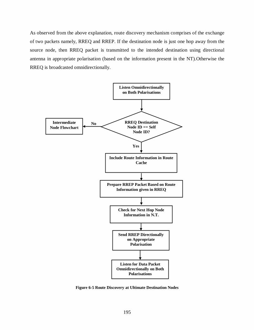
195

As observed from the above explanation, route discovery mechanism comprises of the exchange

of two packets namely, RREQ and RREP. If the destination node is just one hop away from the

source node, then RREQ packet is transmitted to the intended destination using directional

antenna in appropriate polarisation (based on the information present in the NT).Otherwise the

RREQ is broadcasted omnidirectionally.

Figure 6-5 Route Discovery at Ultimate Destination Nodes

Listen Omnidirectionally on Both Polarisations

RREQ Destination Node ID == Self

Node ID?

No Intermediate Node Flowchart

Yes

Include Route Information in Route Cache

Prepare RREP Packet Based on Route Information given in RREQ

Check for Next Hop Node Information in N.T.

Send RREP Directionally on Appropriate

Polarisation

Listen for Data Packet Omnidirectionally on Both

Polarisations

196

Such directional and polarised transmission of RREQ among source and destination node pairs

which are in direct communication range helps in achieving reduced interference and

overcoming exposed node problem for better special reuse of the available spectrum. Similarly,

if an intermediate node finds that the intended destination node is its one hop neighbour, then it

also transmits the RREQ to the destination node directionally in appropriate polarisation.

If the source and destination nodes are not neighbours, then the source node broadcasts the

RREQ omnidirectionally in vertical polarisation. All the intermediate nodes append their node

ID to the RREQ packet. Therefore length of the RREQ packet increases with every hop. No node

transmits the RREQ packet with same request ID twice to ensure loop-free routing. The

information of node IDs of the intermediate nodes is used for route establishment between source

and destination nodes. On receiving the RREQ, the destination node uses the intermediate node

ID information available in the RREQ packet and forms the RREP packet to establish the

backward path. In order to support multipath routing, the destination node sends RREP for every

RREQ received.

Figure 6-6 FSM for Route Discovery Mechanism

The Finite State Machine (FSM) for the route discovery mechanism in DPDA-MRP is presented

in Figure 6-6. As observed from the FSM, when an idle node needs to send data to another node

(destination), it checks if the other node is a neighbour through its NT, or if any route is available

197

in its RT. If the destination node is neither a neighbour, nor any route is available for the same,

then the source node broadcasts RREQ and waits to receive the RREP. If RREP is not received

within the timeout period, the RREQ is retransmitted till retransmission limit is reached. If RREP

is not received even after retransmission limit is reached, the node aborts RREQ transmission

and transits back to idle state. If the node receives the RREP, it updates its route cache.

6.2.2 Route Maintenance in DPDA-MRP

The flowchart for route maintenance in DPDA-MRP is shown in Figure 6-7.Route maintenance

is essential in MANETs because there are chances of route breakage due to mobility of nodes. In

route maintenance phase, nodes exchange RERR packet to inform the source node about route

breakage. The RERR packet is comprised of different fields such as transmitter address (sender

of RERR), receiver address (original source node), node address of next hop in backward path,

sequence number, address of the node which is not reachable and 1 bit field to indicate success

or failure of transmitting the packet on the alternate path (1 on success and 0 on failure). After

route establishment in the route discovery phase, the source node selects minimum hop path as

the best path for data exchange. For communication, nodes exchange RTS, CTS, Data and ACK

frames using directional antenna in appropriate polarisation. This is achieved according to

DPDA-MAC protocol, explained in Chapter 5. Whenever a node transmits or forwards RTS or

Data frame, it waits for CTS or ACK respectively for 110 ms (timeout).

A node transmits the RTS or Data frame using directional antenna in appropriate polarisation and

senses the medium omnidirectionally in same polarisation. If the transmitting node does not

receive expected CTS or ACK till timeout expiration, it checks for next best path to the

destination node in its route cache. The RT is also updated to remove the invalid route from the

RT. If an alternate best path is available, then the transmitting node (intermediate or source) uses

the available alternate path for further communication. If the transmitting node is an intermediate

node, it sends RERR packet to the original source to inform it about route breakage. In this case,

the value of success bit in RERR packet is set to 1 by the intermediate node to inform the

original source node that it could successfully transmit data by using an alternate best path.

198

Figure 6-7 Route Maintenance in DPDA-MRP

The RT is also updated to remove the invalid route from the RT. If an alternate best path is

available, then the transmitting node (intermediate or source) uses the available alternate path for

further communication. If the transmitting node is an intermediate node, it sends RERR packet to

the original source to inform it about route breakage. In this case, the value of success bit in

RERR packet is set to 1 by the intermediate node to inform the original source node that it could

successfully transmit data by using an alternate best path.

Transmit or Forward Data Frame

Listen for CTS/ACK

Timeout Reached?

No

Search Route Cache for Next Best and

Latest Path

Best and Latest Path Available?

Send RERR to Original Source

Directionally with Success Bit OFF

No

Yes

Transmit Data on Best and Latest Available

Path

Send RERR to Original Source

Directionally with Success Bit ON

Yes

199

If the intermediate node fails to find the next best path in its route cache, then it drops the packet

and sends RERR to the original source node with success bit set to 0. It must be noted that RERR

frame is transmitted directionally to avoid interference and achieve better spatial reuse. Also, as

RERR is intended for the original source node, it is not required to be transmitted

omnidirectionally.

Figure 6-8 FSM for Route Maintenance in DPDA-MRP

The FSM for route maintenance in DPDA-MRP is shown in Figure 6-8. When a node receives

RERR frame, it updates its RT and searches the next best path for communication. Data

transmission takes place according to DPDA-MAC protocol explained in Section 5.2 of Chapter

5.

6.3 Formation of Routing Table and Multiple Route Discovery with Mobility of

Nodes

Nodes exchange RREQ, RREP and RERR frames for route discovery and maintenance. All the

nodes maintain RT having multiple routes to nodes which are not their one hop neighbours, and

NT, for nodes which are just one hop away from themselves. An example NT is presented in

Table 4-1 of Chapter 4.

This section presents an example of a RT having multiple routes between source and destination

nodes. Due to mobility of nodes, old routes may become invalid and new routes are formed. To

form RT, a MANET scenario is developed based on the specifications given in Table 6-1.

Simulations are carried out in a simulator developed in C++ and details of the same are presented

in Appendix 1. Main aim of this scenario is to show the formation of RT and change in its entries

with mobility of nodes. Therefore, no data packets are exchanged in this case, and this scenario

200

is not used for performance analysis. Nodes only exchange RREQ and RREP packets for route

discovery based on the proposed DPDA-MRP protocol.

Table 6-1 Scenario Specifications for Simulations to Analyse Route Discovery and RT Formation with DPDA-

MRP

Parameter Value

Channel Bit Rate 11 Mbps

Routing Protocol DPDA-MRP

Communication Range 200 m

Broadcast Frame Length 208 bits

RREQ Frame Length 160 bits +

(hop node ID x no. of

intermediate nodes)

RREP Frame Length Equal to final RREQ frame length

Terrain 500m x 500m

Number of Nodes 9

Node Placement Grid

Inter Node Distance 190m

Mobility Model Random Waypoint Mobility

Speed 3 m/s

Pause Time 0 s

Simulation Time 60 s

Simulation is carried out for channel capacity of 11 Mbps based on IEEE 802.11b standard

(Forouzan 2007). The communication distance is configured to be 200 m for reasons discussed

in Section 3.2. The frame length of broadcast packet is as discussed in Section 4.3. The length of

RREQ and RREP is as discussed in Section 6.2.1. A flat terrain of 500 x 500 m2 is used for

simulation, and 9 nodes are placed in a 3x3 grid topology. Grid topology is used because it is

easy to analyse the paths discovered when nodes are placed in grid topology. Nodes are placed at

a distance of 190 m to ensure that they are within communication range of each other. Random

waypoint mobility model is used for mobility because it is the most popular and frequently used

201

mobility model used in simulation based studies of MANETs (Bai and Helmy 2004) and

(Bettstetter and Wagner 2002). The nodes are simulated to move at a speed of 3 m/s and pause

for 0 s (no pause) to simulate walking and speed of humans. The simulation is run for 60 s to

study the formation of RT and change in its entries with mobility of nodes.

A 9 node scenario based on the specifications given in Table 6-1, is represented in Figure 6-9.

The x and y coordinates of the nodes are mentioned next to the nodes to notify their location. For

example, in Figure 6-9, the x, y coordinates of Node 0 are 0 m and 380 m respectively. As the

communication distance between the nodes is 200 m, all the nodes which are 190 m apart

become each other’s neighbour and can be reached in single hop.

Figure 6-9 Initial Node Placement

The entries of RT for Nodes 8 and 2 at Node 0 are presented in Table 6-2. The RT consists of

information about source node, destination node, number of paths discovered from source to

destination, information about the path and path size (number of hops). As observed from the

Table 6-2, at 5 s, 10 paths are discovered from Node 0 to Node 8, while 6 paths are discovered

from Node 0 to Node 2.

Change in routes due to mobility of nodes can be observed from Table 6-3, which shows the

entries of RT at 40 s. It must be observed from the Table 6-3, that Node 2 is now one hop

neighbour of Node 0 and therefore there are routes present for the same. For communication with

Node 2, Node 0 will refer to the information present in its NT.

202

Table 6-2 Routing Table Entries at Node 0 for Nodes 8 and 2 at 5 s

Source

Node

Destination

Node

Number of

Paths Found

Path(s) Path Size

0 8 10 1-2-5-8

1-4-7-8

1-4-5-8

3-6-7-8

3-4-7-8

3-4-5-8

1-2-5-4-7-8

3-4-1-2-5-8

3-6-7-4-5-8

1-2-5-4-3-6-7-8

3

3

3

3

3

3

5

5

5

7

0 2 6 1-2

3-4-5-2

3-4-1-2

3-4-7-8-5-2

3-6-7-8-5-2

3-6-7-4-5-2

1

3

3

5

5

5

Table 6-3 Routing Table Entries at Node 0 for Nodes 8 and 2 at 40 s

Source Node Destination

Node

Number of

Paths Found

Path(s) Path

Size

0 8 4 4-5-8

2-5-8

4-7-8

1-2-5-8

2

2

2

3

0 2 Entry in Neighbour Table

6.4 Route Disjointness in DPDA-MRP

Most of the multipath routing protocols analysed in the literature discover node-disjoint or link-

disjoint routes. In node-disjoint routes, neither node nor links are shared among different routes.

Therefore, particular sets of nodes and links are exclusively used for communication between a

source-destination pair. However, as reported in (Waharte and Boutaba 2006), when the

networks become sparse, and inter-node distance increases, discovery of node-disjoint paths

becomes difficult. An example of node-disjoint routes is shown in Figure 6-10.

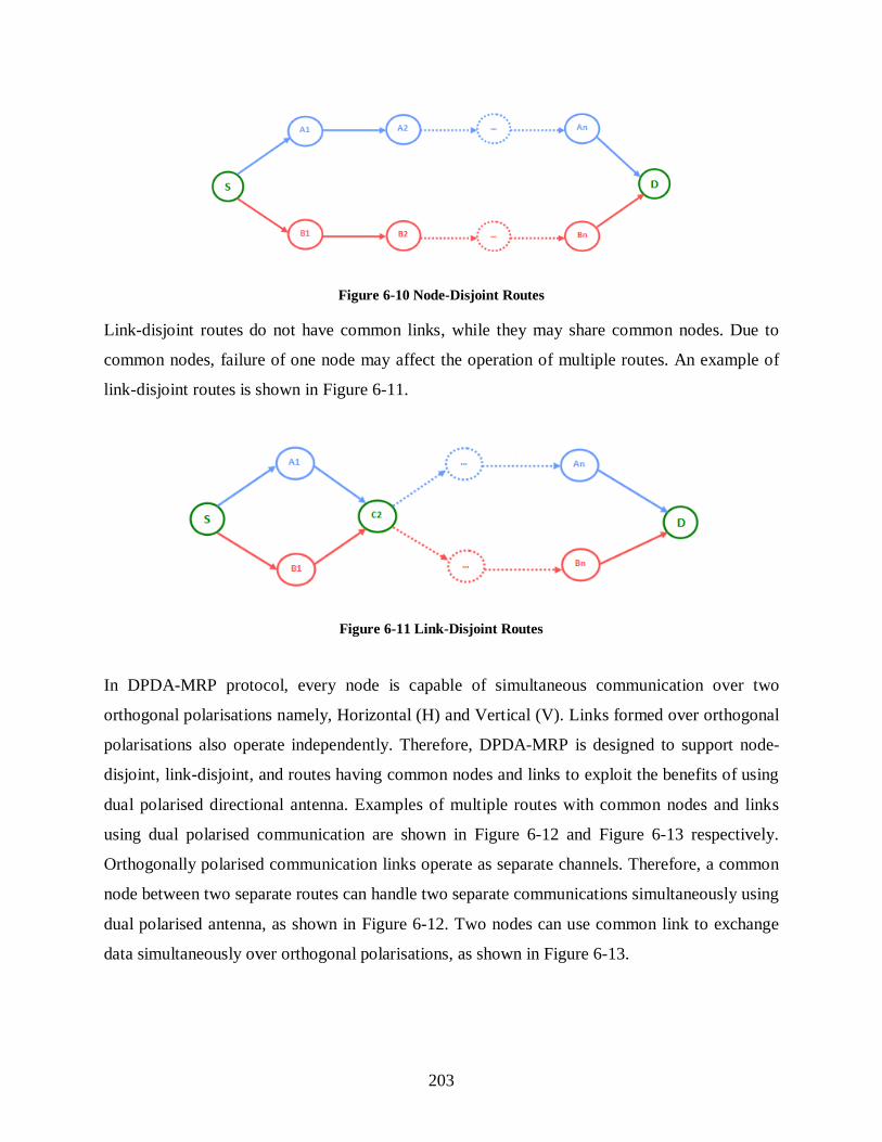
203

Figure 6-10 Node-Disjoint Routes

Link-disjoint routes do not have common links, while they may share common nodes. Due to

common nodes, failure of one node may affect the operation of multiple routes. An example of

link-disjoint routes is shown in Figure 6-11.

Figure 6-11 Link-Disjoint Routes

In DPDA-MRP protocol, every node is capable of simultaneous communication over two

orthogonal polarisations namely, Horizontal (H) and Vertical (V). Links formed over orthogonal

polarisations also operate independently. Therefore, DPDA-MRP is designed to support node-

disjoint, link-disjoint, and routes having common nodes and links to exploit the benefits of using

dual polarised directional antenna. Examples of multiple routes with common nodes and links

using dual polarised communication are shown in Figure 6-12 and Figure 6-13 respectively.

Orthogonally polarised communication links operate as separate channels. Therefore, a common

node between two separate routes can handle two separate communications simultaneously using

dual polarised antenna, as shown in Figure 6-12. Two nodes can use common link to exchange

data simultaneously over orthogonal polarisations, as shown in Figure 6-13.

204

Figure 6-12 Routes with Common Nodes using Dual Polarised Communication

Figure 6-13 Routes with Common Links using Dual Polarised Communication

As mentioned earlier, DPDA-MRP is designed to exploit the benefits of dual polarisation to

attain high data rates and throughput by simultaneous use of orthogonal polarisations. Also, since

there are no restrictions/limitations of discovering node or link-disjoint routes, DPDA-MRP is

fast and more efficient in route discovery when compared to other multipath routing protocols

which look for disjoint routes.

To demonstrate simultaneous communication over vertical and horizontal polarisations on node-

disjoint, link-disjoint and routes having common nodes and links, experiments are conducted

based on scenario specifications given in Table 6-4. These simulations are carried out in a

simulator developed in C++ and details of the same are presented in Appendix 1. Here, 4-8 node

scenarios have been considered to demonstrate simultaneous communication over multiple

routes with different degrees of disjointness by tracing the flow of packets over every hop. These

scenarios are not used for performance analysis. The scenario specifications in Table 6-4 are

same those in Table 6-1, except that nodes in these scenarios are placed manually to enable

formation of node disjoint, links disjoint, routes with common nodes and routes with common

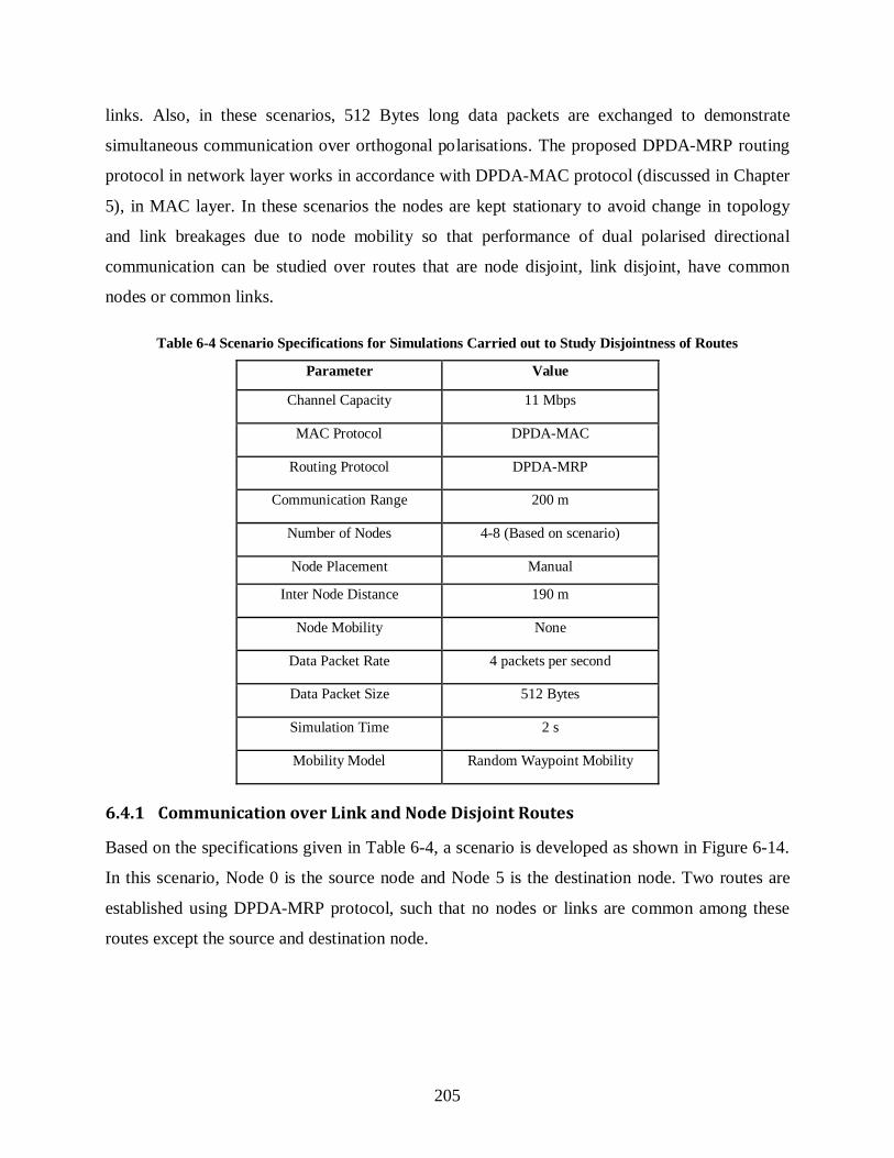
205

links. Also, in these scenarios, 512 Bytes long data packets are exchanged to demonstrate

simultaneous communication over orthogonal polarisations. The proposed DPDA-MRP routing

protocol in network layer works in accordance with DPDA-MAC protocol (discussed in Chapter

5), in MAC layer. In these scenarios the nodes are kept stationary to avoid change in topology

and link breakages due to node mobility so that performance of dual polarised directional

communication can be studied over routes that are node disjoint, link disjoint, have common

nodes or common links.

Table 6-4 Scenario Specifications for Simulations Carried out to Study Disjointness of Routes

Parameter Value

Channel Capacity 11 Mbps

MAC Protocol DPDA-MAC

Routing Protocol DPDA-MRP


Number of Nodes 4-8 (Based on scenario)

Node Placement Manual

Inter Node Distance 190 m

Node Mobility None

Data Packet Rate 4 packets per second

Data Packet Size 512 Bytes

Simulation Time 2 s

Mobility Model Random Waypoint Mobility

6.4.1 Communication over Link and Node Disjoint Routes

Based on the specifications given in Table 6-4, a scenario is developed as shown in Figure 6-14.

In this scenario, Node 0 is the source node and Node 5 is the destination node. Two routes are

established using DPDA-MRP protocol, such that no nodes or links are common among these

routes except the source and destination node.

206

Figure 6-14 Node-Disjoint and Link-Disjoint Routes

Figure 6-15 Timeline for Per Hop Exchange of Packets for Node-Disjoint and Link-Disjoint Routes

Communication over route 0-1-2-5 takes place directionally using horizontal polarisation (H)

and while communication over route 0-3-4-5 takes place directionally using vertical polarisation

(V). Nodes 0 and 5 simultaneously use both the polarisations for directional communication

over both the routes. While Node 0 transmits data directionally over vertical and horizontal

polarisations simultaneously, Node 5 receives data over vertical and horizontal polarisations

simultaneously using directional antenna.

The timeline for per hop exchange of packets over two node-disjoint and link-disjoint paths

using orthogonal polarisations for directional communication between the nodes is shown in

Figure 6-15. From the timeline it is observed that with the use of orthogonal polarisations,

simultaneous exchange of packets can take place over both the polarisations, which can help in

attaining enhanced data throughput.

207

Figure 6-16 Simultaneous Communication over Orthogonal Polarisations for Node-Disjoint and Link-

Disjoint Routes

The overlap in time for communication over two node and link-disjoint routes using orthogonal

polarisations for exchange of information is shown in Figure 6-16. Use of dual polarised

directional antenna helps in overcoming the problems of interference and exposed nodes, thus

enhancing network performance and efficiency.

6.4.2 Communication over Routes with Common Node

The scenario in Figure 6-17 shows two routes with one common node. Here, Node 0 is the

source node and Node 6 is the destination node.

Figure 6-17 Routes with Common Node

Two routes established between the source and destination nodes are 0-2-4-3-6 and 0-1-4-5-6.

Communication over route 0-2-4-3-6 takes place directionally using vertical polarisation (V),

while communication over route 0-1-4-5-6 takes place directionally using horizontal polarisation

(H). Nodes 0, 4 and 6 simultaneously use both the polarisations for dual polarised directional

communication.

208

Figure 6-18 Timeline for Per Hop Exchange of Packets for Routes with Common Node

Figure 6-19 Simultaneous Communication over Orthogonal Polarisations for Routes with Common Nodes

The timeline for simultaneous exchange of packets over two routes is shown in Figure 6-18.

From this information it must be noted that DPDA-MRP exploits the benefits of dual polarised

directional communication even in the presence of common nodes between multiple paths. The

overlap in time for communication carried out over vertical and horizontal polarisations is shown

in Figure 6-19.

From the timing information presented in Figure 6-18 and Figure 6-19, it can be concluded that

while other multipath routing protocols consider the presence of common nodes as a drawback,

for DPDA-MRP this is not the case.

209

6.4.3 Communication over Routes with Common Link

In the scenario shown in Figure 6-20, communication takes place over route 0-2-3 using vertical

polarisation and over route 1-2-3 using horizontal polarisation. Node 2 communicates with Node

3 by simultaneously using orthogonal polarisations over the same communication link.

Figure 6-20 Communication over Common Link

Node 2 receives data from Node 0 over vertical polarisation and that from Node 1 over

horizontal polarisation. It transmits the data received from Node 0 and Node 1 over vertical and

horizontal polarisations respectively to Node 3. In case Nodes 2 and 3 were not capable of dual

polarised directional communication, the link between these nodes could have faced congestion

and Node 2 could have become a bottleneck due to simultaneous traffic from Nodes 0 and 1.

Figure 6-21 Timeline for Per Hop Exchange of Packets for Common Link

The timeline for simultaneous exchange of packets using vertical and horizontal polarisations

over the common link existing between Nodes 2 and 3 is shown in Figure 6-21. The overlap in

time for the communication carried out over common link between Nodes 2 and 3 is presented in

Figure 6-22.Nodes 2 and 3 use dual polarised directional antennas for simultaneous transmission

and reception of information over orthogonal polarisations, without interference.

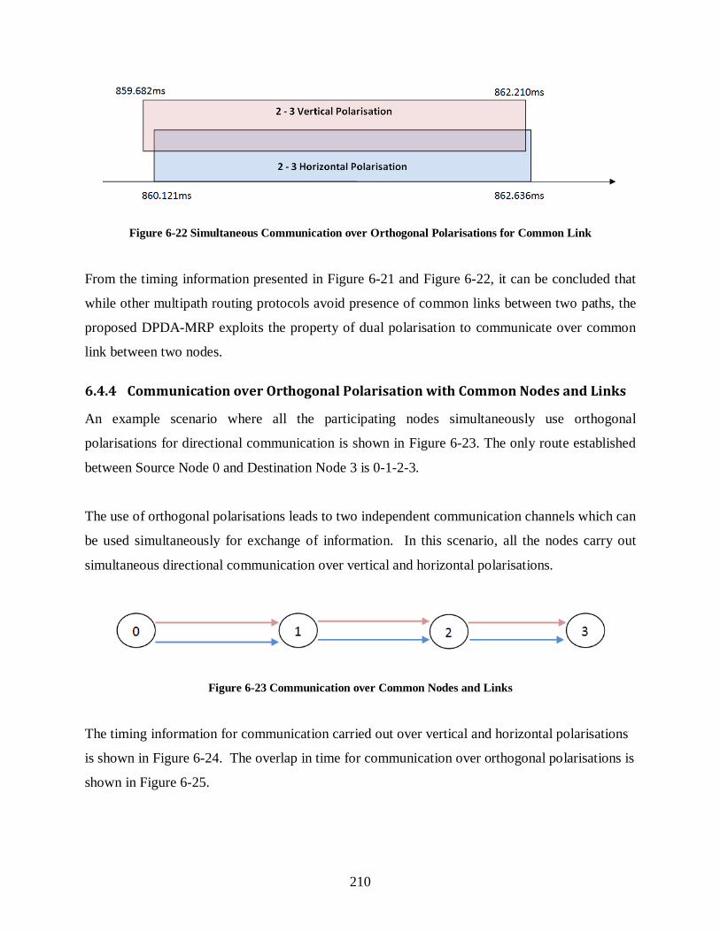
210

Figure 6-22 Simultaneous Communication over Orthogonal Polarisations for Common Link

From the timing information presented in Figure 6-21 and Figure 6-22, it can be concluded that

while other multipath routing protocols avoid presence of common links between two paths, the

proposed DPDA-MRP exploits the property of dual polarisation to communicate over common

link between two nodes.

6.4.4 Communication over Orthogonal Polarisation with Common Nodes and Links

An example scenario where all the participating nodes simultaneously use orthogonal

polarisations for directional communication is shown in Figure 6-23. The only route established

between Source Node 0 and Destination Node 3 is 0-1-2-3.

The use of orthogonal polarisations leads to two independent communication channels which can

be used simultaneously for exchange of information. In this scenario, all the nodes carry out

simultaneous directional communication over vertical and horizontal polarisations.

Figure 6-23 Communication over Common Nodes and Links

The timing information for communication carried out over vertical and horizontal polarisations

is shown in Figure 6-24. The overlap in time for communication over orthogonal polarisations is

shown in Figure 6-25.

211

Figure 6-24 Timeline for Per Hop Exchange of Packets over Common Nodes and Links

Figure 6-25 Simultaneous Communication over Orthogonal Polarisations for Common Nodes and Links

From the time information presented in Figure 6-24 and Figure 6-25, it can be observed that,

unlike other protocols available in literature, the proposed DPDA-MRP can use common nodes

and links to carry out independent simultaneous communication over orthogonal polarisations.

6.5 Conclusion

This chapter presented detailed design of the DPDA-MRP protocol. DPDA-MRP is a multipath

routing protocol based on dual polarised directional communication. It is composed of two

phases namely route discovery phase and route maintenance phase. Since DPDA-MRP supports

discovery of multiple routes between source and destination nodes, it provides robust and

reliable communication against mobility of nodes. DPDA-MRP is a hybrid routing protocol

wherein NT is formed proactively with periodic exchange of broadcast packets and routing

tables are formed reactively through exchange of RREQ, RREP and RERR packets for route

discovery and maintenance. Nodes using DPDA-MRP for routing of information are capable of

dual polarised communication, based on which a node can simultaneously communicate with

212

two different nodes using two orthogonal polarisations. This property renders DPDA-MRP to

support establishment of node-disjoint, link-disjoint, non node-disjoint, non link-disjoint and

routes with common nodes and links. This functionality of DPDA-MRP has been verified

through simulations. With DPDA-MRP, nodes can establish routes over vertical and horizontal

polarisations simultaneously, and there is no need for considering node or link disjointness

during discovery of routes. Through simulations, it is observed that with the help of dual

polarised communication, simultaneous exchange of information can take place over different

routes and links between source and destination nodes in MANET. By virtue of the dual

polarised directional communication, DPDA-MRP can be categorised as a non-disjoint and zone-

disjoint, multipath routing protocol. DPDA-MRP is a multipath routing protocol which is

supported by DPDA-MAC for access to the medium.

213

CHAPTER 7

7 Performance Analysis of DPDA-MRP, SPDA-MRP and DSR

7.1 Introduction

In this chapter, the performance of three routing protocols namely DPDA-MRP, Single Polarised

Directional Antenna based Multipath Routing Protocol (SPDA-MRP) and Dynamic Source

Routing (DSR) is studied. The performance of these protocols is analysed in terms of PDR and

throughput. The results obtained through simulations are presented and analysed.

As discussed in Chapter 6, the proposed DPDA-MRP protocol uses dual polarised directional

antenna for communication between the nodes, along with support for multipath routing.

However, to appreciate the importance of using dual polarised directional antenna for routing of

information, the performance of DPDA-MRP is compared with that of other routing protocols

which use single polarisation based directional communication and single polarisation based

omnidirectional communication. For this, the performance of DPDA-MRP protocol is compared

with that of Single Polarised Directional Antenna based Multipath Routing Protocol (SPDA-

MRP) and Dynamic Source Routing (DSR) protocol (Johnson, Maltz and Broch 2001).

The SPDA-MRP uses directional antenna with only vertical polarisation available for

communication. SPDA-MRP is the network layer extension of SPDA-MAC protocol, which is

explained in Section 5.4 of Chapter 5. Like DPDA-MRP, SPDA-MRP protocol also exchanges

periodic Link ID broadcast packets to maintain NT. The NT maintains information about free

and busy polarisations and their NAV durations. This information is used to overcome the

problem of deafness. However, like in SPDA-MAC, SPDA-MRP uses only one polarisation

(vertical polarisation) for discovery of routes and routing of information in MANETs. Therefore,

while in DPDA-MRP a node can maintain routes and carry out routing of information over both

vertical and horizontal polarisations, in SPDA-MRP nodes maintain routes and carry out routing

of information only in vertical polarisation. The method of discovery of multiple routes between

nodes and their maintenance in SPDA-MRP is same as that of DPDA-MRP.

214

The Dynamic Source Routing (DSR) protocol uses omnidirectional communication in vertical

polarisation.DSR is also a multipath routing protocol which discovers multiple paths between

source and destination nodes reactively. The method of route discovery and maintenance used in

DPDA-MRP and SPDA-MRP is based on DSR. The MAC layer protocol used for DSR is

CSMA/CA which is explained in Section 2.6.3, and its performance is compared with that of

DPDA-MAC and SPDA-MAC in Chapter 5.

While all the protocols support multipath routing, in DPDA-MRP the nodes can communicate

directionally over two orthogonal polarisations (vertical and horizontal). Though nodes in

SPDA-MRP also communicate directionally, it uses only single polarisation (vertical).

Comparative study between DPDA-MRP and SPDA-MRP is aimed to analyse and appreciate the

difference in performance when two polarisations are used for directional communication and

when only one polarisation is used for directional communication. DSR uses omnidirectional

communication over single (vertical) polarisation. Inclusion of DSR in this comparative study is

to highlight the advantages of directional communication over omnidirectional communication

mainly in combating the exposed node problem. Therefore, this study is aimed at analysing the

performance of a network which uses multipath routing protocol with dual polarised directional

communication through DPDA-MRP, single polarised directional communication through

SPDA-MRP and single polarised omnidirectional communication through DSR.

The simulations are carried out in a simulator developed in C++ and details of the same are

presented in Appendix 1. The specifications for different scenarios are shown in Table 7-1. The

scenario specifications in Table 7-1 are same as those in Table 5-2, except for the inclusion of

routing protocols DPDA-MRP, SPDA-MRP and DSR, which work with corresponding MAC

layer protocols (DPDA-MAC, SPDA-MAC and CSMA/CA respectively). Reasons for

considering the parameters for simulation are same as given for Table 5-2.

In the developed scenario, the terrain size is maintained as 1000 x 1000 m2 and the number of

nodes is increased from 20 to 100, in steps of 20 nodes. At different node densities, 25 % of the

nodes are transmitters and another 25% are the receivers, as mentioned in Table 7-1.

215

Table 7-1 Scenario Specifications for Simulations to Study the Performance of DPDA-MRP, SPDA-MRP and

DSR

Parameter Value

Terrain Size 1000 x 1000 m2

Number of Nodes 20, 40, 60, 80 and 100

Number of Transmitters 05, 10, 15, 20 and 25


Number of Receivers 05, 10, 15, 20 and 25


Node Placement Random

Routing Protocol DPDA-MRP, SPDA-MRP, DSR

Node Mobility Random Waypoint

Speed 0, 1, 2, 3 m/s

Pause Time 4s


Packets Per Second 1, 5, 15, 25

Channel Capacity 2, 11 and 54 Mbps

Probability of Error 5%

Simulation Time 100 s


Threshold SNR 10 dB

Number of Seeds 50

The increased density of nodes leads to increase in interference and exposed node problem, and

is used to study the performance of dual-polarised directional antenna based DPDA-MRP, single

polarised directional antenna based SPDA-MRP, and omnidirectional antenna based DSR for

communication between mobile nodes.

Mobility of nodes is based on the random waypoint mobility model and performance of the

protocols is tested with stationary nodes (speed of 0m/s), and nodes moving at speed of 1 m/s, 2

m/s and 3 m/s with a pause time of 4s to simulate walking and running speed of human. Each

data packet is 1024 Bytes (1 kB) long. Rate of packet transmission is varied as 1 packet per

second, 5 packets per second, 15 packets per second and 25 packets per second to study the

216

effect of variation in data rate on performance of the simulated protocols. Simulations are carried

out over different channel capacities of 2 Mbps, 11 Mbps and 54 Mbps. Simulations are carried

out for 50 seeds and average of 50 runs is taken to plot the graphs for different performance

parameters. Performance of the protocols is studied in terms of Packet Delivery Ratio (PDR) and

Throughput. In the following sections, results obtained through simulations are presented and

analysed. The results are presented along with standard deviation for all the three protocols.

7.2 Effect of Variation in Density and Mobility of Nodes on PDR Achieved by DPDA-

MRP, SPDA-MRP and DSR with Varying Rate of Packet Transmission

PDR represents the number of packets retrieved successfully at the receiver over the simulation

time of 100 s. The available channel capacity and number of nodes trying to access the network,

play an important role in the PDR performance achieved by a routing protocol. This section

presents the variation in the PDR achieved by DPDA-MRP, SPDA-MRP and DSR, by varying

the rate of packet transmission, mobility of nodes and density of nodes in a given area. The rate

of packet transmission is varied as 1 packet per second, 5 packets per second, 15 packets per

second and 25 packets per second. For a given rate of packet transmission, performance of the

routing protocols is measured with varying mobility of nodes, density of nodes and capacity of

the communication channel. As mentioned in Table 7-1, mobility of nodes is varied from 0 m/s

to 3 m/s, in steps of 1 m/s. Density of nodes is varied from 20 nodes per unit area to 100 nodes

per unit area, in steps of 20. Three different channel capacities of 2 Mbps, 11 Mbps and 54 Mbps

are used for analysing the performance of the routing protocols.

7.2.1 Analysis of Variation in PDR of DPDA-MRP

This section presents the variation in the performance of DPDA-MRP in terms of PDR. PDR of

DPDA-MRP is studied for the packet transmission rates of 1 packet per second, 5 packets per

second, 15 packets per second and 25 packets per second. PDR is measured with varying node

density. This study presents the effect of varying node density on network performance when

DPDA-MRP is used for routing of information. Density of nodes is varied from 20 nodes per

unit area to 100 nodes per unit area, in steps of 20. Mobility of nodes is varied from 0 m/s

(stationary nodes), to 3 m/s in steps of 1, to simulate the walking and running speed of humans.

The performance of DPDA-MRP is studied at channel capacities of 2 Mbps, 11 Mbps and 54

Mbps.

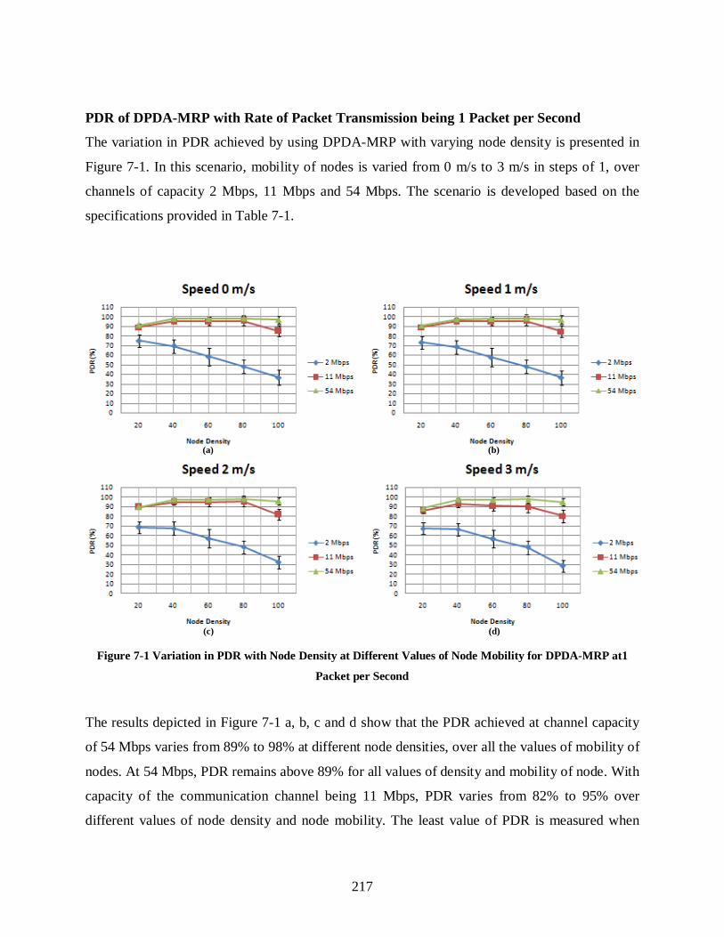
217

PDR of DPDA-MRP with Rate of Packet Transmission being 1 Packet per Second

The variation in PDR achieved by using DPDA-MRP with varying node density is presented in

Figure 7-1. In this scenario, mobility of nodes is varied from 0 m/s to 3 m/s in steps of 1, over

channels of capacity 2 Mbps, 11 Mbps and 54 Mbps. The scenario is developed based on the

specifications provided in Table 7-1.

Figure 7-1 Variation in PDR with Node Density at Different Values of Node Mobility for DPDA-MRP at1

Packet per Second

The results depicted in Figure 7-1 a, b, c and d show that the PDR achieved at channel capacity

of 54 Mbps varies from 89% to 98% at different node densities, over all the values of mobility of

nodes. At 54 Mbps, PDR remains above 89% for all values of density and mobility of node. With

capacity of the communication channel being 11 Mbps, PDR varies from 82% to 95% over

different values of node density and node mobility. The least value of PDR is measured when

(a) (b)

(c) (d)

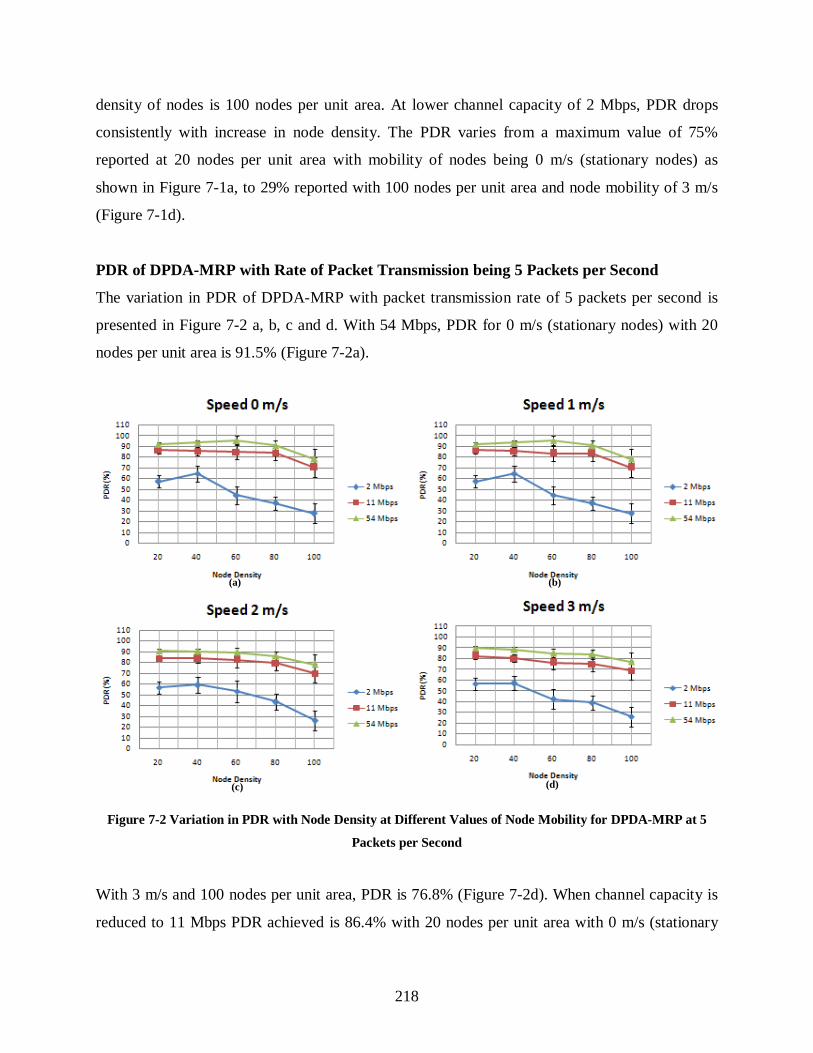
218

density of nodes is 100 nodes per unit area. At lower channel capacity of 2 Mbps, PDR drops

consistently with increase in node density. The PDR varies from a maximum value of 75%

reported at 20 nodes per unit area with mobility of nodes being 0 m/s (stationary nodes) as

shown in Figure 7-1a, to 29% reported with 100 nodes per unit area and node mobility of 3 m/s

(Figure 7-1d).

PDR of DPDA-MRP with Rate of Packet Transmission being 5 Packets per Second

The variation in PDR of DPDA-MRP with packet transmission rate of 5 packets per second is

presented in Figure 7-2 a, b, c and d. With 54 Mbps, PDR for 0 m/s (stationary nodes) with 20

nodes per unit area is 91.5% (Figure 7-2a).

Figure 7-2 Variation in PDR with Node Density at Different Values of Node Mobility for DPDA-MRP at 5

Packets per Second

With 3 m/s and 100 nodes per unit area, PDR is 76.8% (Figure 7-2d). When channel capacity is

reduced to 11 Mbps PDR achieved is 86.4% with 20 nodes per unit area with 0 m/s (stationary

(a)

(c) (d)

(b)

219

nodes) as shown in Figure 7-2a. PDR drops to 68.8% with increase in node density to 100 nodes

per unit area and node mobility being 3 m/s (Figure 7-2d). At channel capacity of 2 Mbps, the

maximum measured PDR is 64.5% when density of nodes is 40 nodes per unit area for mobility

of nodes being 0 m/s and 1 m/s as shown in Figure 7-2a and Figure 7-2b respectively. It drops to

25.8% at node density of 100 nodes per unit area and mobility of 3 m/s as shown in Figure 7-2d.


The performance of DPDA-MRP at transmission rate of 15 packets per second is studied in

terms of PDR by varying the density and mobility of nodes. Results are presented in Figure 7-3.


Packets per Second

At the channel capacity of 54 Mbps, it is observed that PDR first increases with increase in node

density and then drops when density of nodes is increased further for all values of mobility of

nodes. When nodes move at 3 m/s, PDR increases from 49% with 20 nodes per unit area, to

77.7% with 60 nodes per unit area (Figure 7-3 d). With increase in node density to 100 nodes per

(a)

(c) (d)

(b)

220

unit area PDR drops to 54% (Figure 7-3 d).Similar trend is observed with the channel capacity of

11 Mbps for all values of node mobility. When the nodes move at 3 m/s, PDR increases with

increase in node density up to 60 nodes per unit area and then starts to drop. The PDR is 43%

with node density of 20 nodes per unit and increases up to 62.6% for the node density of 60

nodes per unit area at node mobility of 3 m/s (Figure 7-3d). It drops to approximately 49% when

the density of nodes increases to 100 nodes per unit area. When the capacity of channel is

reduced to 2 Mbps, PDR also reduces, as expected. Drop in PDR is also observed with increase

in mobility of nodes. When the nodes move at 3 m/s, PDR increases with increase in density of

nodes from 20 nodes per unit area to 40 nodes per unit area. It reduces consistently with further

increase in node density (Figure 7-3d). While the PDR computed with 20 nodes per unit area is

22.6%, it increases to 31% with node density of 60 nodes per unit area and then drops to 11.8%

for node density of 100 nodes per unit area (Figure 7-3d).


The rate of packet transmission is increased to 25 packets per second to study the effect of

further increase in the rate of packet transmission on the performance of DPDA-MRP in terms of

PDR. The variation in PDR with varying node density, mobility of nodes and channel capacity is

presented in Figure 7-4.

At channel capacity of 54 Mbps, for all values of node mobility, PDR first increases with

increase in node density and then starts to deteriorate when density of nodes is increased further.

When nodes move at 3 m/s (Figure 7-4 d), the PDR measured for the node density of 20 nodes

per unit area is 38.7% and it increases to 57% when node density is increased to 40 nodes per

unit area. With further increase in node density to 100 nodes per unit area, PDR drops to 44%

(Figure 7-4 d).

PDR achieved with the channel capacity of 11 Mbps is less than that of 54 Mbps, which is as

expected. With node mobility of 3 m/s, PDR measured with 20 nodes per unit area is 32.2%.

221


Packets per Second

It improves to 47.3% when density of nodes increases to 80 nodes per unit area (Figure 7-4 d).

When node density increases to 100 nodes per unit area, PDR degrades to 38.3% (Figure 7-4 d).

When channel capacity is reduced to 2 Mbps, PDR constantly degrades with increase in density

of nodes for node mobility of 0 m/s, 1 m/s and 2 m/s. With node mobility of 3 m/s, PDR with 20

nodes per unit area is 17.4% (Figure 7-4 d). It increases slightly to 18.5% for node density of 40

nodes per unit area. With further increase in node density, PDR deteriorates. It drops to 6.4%

with node density of 100 nodes per unit area (Figure 7-4 d).

Values of Standard Deviation (SD) with respect to Mean (M) for DPDA-MRP PDR are


for packet transmission rates of 1 and 25 Packets per Second, node mobility of 0 m/s and 3 m/s,

and for selected values of node density. The Mean (M) denotes the values of PDR (%), plotted

(a)

(d) (c)

(b)

222

in the results presented in Figure 7-1 (for rate of 1 Packet per Second) and Figure 7-4 (for rate of

25 Packets per Second).

Table 7-2 Standard Deviation with respect to Mean for DPDA-MRP PDR

DPDA-MRP PDR 1 Packet per Second


0 m/s 3 m/s 0 m/s 3 m/s 0 m/s 3 m/s


20 75 6.7 67.5 6 89 2.2 86.4 3 91.3 1.1 88.4 1.2

60 58.4 9.3 56.7 9 95.2 4.2 91 5 97.7 2.2 97.3 2.3

100 37 7.7 29 6 85.2 5.9 80.6 6.4 97 4 95 4

DPDA-MRP PDR 25 Packets per Second


0 m/s 3 m/s 0 m/s 3 m/s 0 m/s 3 m/s


20 25.2 6.3 17.4 4.3 38 3.8 32.2 3.2 44.3 3.1 38.7 2.7

60 19 5.7 18.2 5.5 54.7 8.4 44.1 6.8 68.5 7.1 57 6

100 9.8 5.2 6.5 5.6 50.2 12.8 38.4 11.5 55.9 12.4 43.5 13

From the results obtained at different rates of packet transmission (Figure 7-1 to Figure 7-4), and

values of standard deviation in Table 7-2 following inferences can be drawn:

1. PDR obtained at the channel capacity of 54 Mbps is the highest, and that obtained at 2

Mbps is the least. This is as expected, because higher the channel capacity, higher will be

the rate of data transmission, leading to higher PDR

2. Generally, with increase in mobility of nodes, routes break and PDR drops. However,

DPDA-MRP being a multipath routing protocol using orthogonal polarisations for

simultaneous data transmission with availability of backup routes, ensures that there is no

degradation in PDR with mobility of nodes

3. PDR first increases with increase in node density and then deteriorates when density of

nodes is increased further. This is mainly due to the fact that with increase in density of

223

nodes, number of communicating nodes increases leading to increase in PDR. DPDA-

MRP simultaneously uses two orthogonal polarisations for communication. Therefore,

higher the number of active nodes, better is the PDR. However, beyond certain value of

node density network congestion starts, leading to deterioration of PDR

4. PDR reduces with increase in rate of packet transmission. This is because of the increase

in network traffic with increase in packet rate, which can lead to queuing delays at

intermediate hops. This can also give rise to network congestion leading to reduction in

PDR.

5. From the values of standard deviation for PDR presented in Table 7-2 it is observed that

standard deviation increases with increase in traffic load. Traffic load on the network

increases due to increase in rate of packet transmission and node density. High traffic

load on the network increases the instances of random backoff delays among the nodes

trying to access the shared medium. This leads to variation in the number of packets

exchanged over the medium for given duration of simulation, causing the PDR across

different seeds to vary. In cases with less traffic load, standard deviation is less because

in such cases, the medium is capable to handle the traffic. This leads to lesser instances of

random backoff among the nodes trying to access the shared medium. Hence, variation of

PDR across different seeds is less, leading to less standard deviation

6. In some cases the absolute value of standard deviation at high node density is lesser than

that a lower node density. However, when expressed as a percentage of its corresponding

mean, the standard deviation with respect to mean is more.

7.2.2 Analysis of Variation in PDR of SPDA-MRP

In this section, variation in the performance of SPDA-MRP is studied in terms of PDR. The

performance is measured at packet transmission rates of 1 packet per second, 5 packets per

second, 15 packets per second and 25 packets per second. The performance is analysed for

different values of density of nodes to study the effect of varying node density on performance of

the network when SPDA-MRP is used for routing of information. Density of nodes is varied

from 20 nodes per unit area to 100 nodes per unit area, in steps of 20. Mobility of nodes is varied

224

from 0 m/s (stationary nodes), to 3 m/s in steps of 1, to simulate the walking and running speed

of humans. The performance of SPDA-MRP is studied at channel capacities of 2 Mbps, 11 Mbps

and 54 Mbps.

PDR of SPDA-MRP with Rate of Packet Transmission being 1 Packet per Second

The variation in PDR when SPDA-MRP is used with varying density and mobility of nodes at

different channel capacities is presented in Figure 7-5.

Figure 7-5 Variation in PDR with Node Density at Different Values of Node Mobility for SPDA-MRP at 1

Packet per Second

At channel capacity of 54 Mbps, with node mobility of 3 m/s, the PDR obtained with 20 nodes

per unit area is 90.4% and that with 100 nodes per unit area is 35% (Figure 7-5 d).

At 11 Mbps, when nodes move at 3 m/s (Figure 7-5 d), the PDR with 20 nodes per unit area is

87%, and drops to 28% node density is increased to 100 nodes per unit area. With channel

capacity of 2 Mbps, and mobility of 3 m/s, PDR with 20 nodes per unit area is 64.4% and it

reduces to 24.8% with 100 nodes per unit area (Figure 7-5d).

(a)

(c) (d)

(b)

225

PDR of SPDA-MRP with Rate of Packet Transmission being 5 Packets per Second

In this section, the variation in PDR achieved with the use of SPDA-MRP is presented. The PDR

for SPDA-MRP, with increased packet rate of 5 packets per second over different values of

channel capacities is presented in Figure 7-6.


Packets per Second

It is observed that PDR drops consistently with increase in node density for all values of mobility

of nodes. At the channel capacity of 54 Mbps, with node mobility being 3 m/s, the PDR with 20

nodes per unit area is 76.8% and reduces to 26.7% with increase in node density to 100 nodes per

unit area (Figure 7-6d). At the channel capacity of 11 Mbps, when nodes move at 3 m/s, PDR

with 20 nodes per unit area is 72.7% and drops to 22.5% at node density of 100 nodes per unit

area (Figure 7-6d). At channel capacity of 2 Mbps, and node mobility of 3 m/s, the PDR with 20

nodes per unit area is 58.4% and that with 100 nodes per unit area is 6.2% (Figure 7-6d).

(a)

(d) (c)

(b)

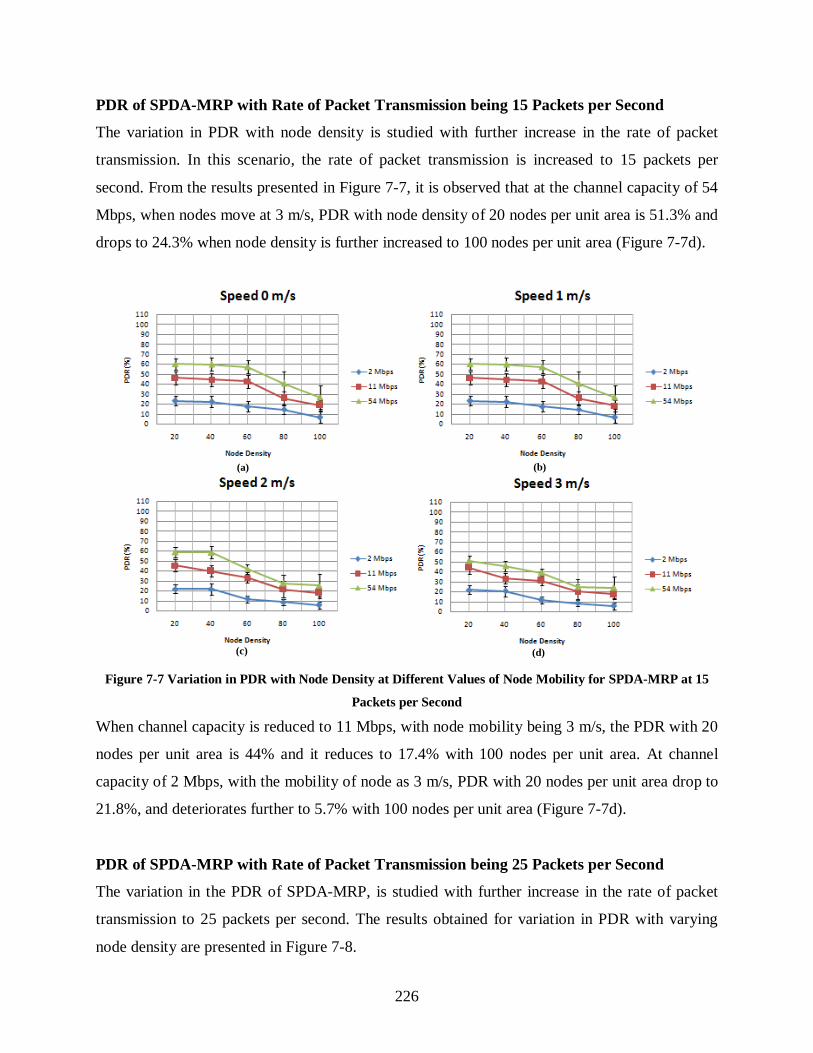
226


The variation in PDR with node density is studied with further increase in the rate of packet

transmission. In this scenario, the rate of packet transmission is increased to 15 packets per

second. From the results presented in Figure 7-7, it is observed that at the channel capacity of 54

Mbps, when nodes move at 3 m/s, PDR with node density of 20 nodes per unit area is 51.3% and

drops to 24.3% when node density is further increased to 100 nodes per unit area (Figure 7-7d).


Packets per Second

When channel capacity is reduced to 11 Mbps, with node mobility being 3 m/s, the PDR with 20

nodes per unit area is 44% and it reduces to 17.4% with 100 nodes per unit area. At channel

capacity of 2 Mbps, with the mobility of node as 3 m/s, PDR with 20 nodes per unit area drop to

21.8%, and deteriorates further to 5.7% with 100 nodes per unit area (Figure 7-7d).


The variation in the PDR of SPDA-MRP, is studied with further increase in the rate of packet

transmission to 25 packets per second. The results obtained for variation in PDR with varying

node density are presented in Figure 7-8.

(a)

(d) (c)

(b)

227

Figure 7-8Variation in PDR with Node Density at Different Values of Node Mobility for SPDA-MRP at 25

Packets per Second

At channel capacity of 54 Mbps, the PDR is 40% with nodes moving at 3 m/s, and node density

being 20 nodes per unit area. PDR increases to 43.6% with 40 nodes per unit area and drops to

19% with 100 nodes per unit area (Figure 7-8d). The increase in PDR when node density

increases to 40 nodes per unit area is due to increase in the number of communicating nodes, due

to increased node density. This increase in the number of communicating nodes along with

higher rate of packet transmission and channel capacity, leads to increase in the PDR. However,

after this limit, PDR starts to drops because SPDA-MRP cannot handle increase in network

traffic. When channel capacity is reduced to 11 Mbps, and nodes move at the speed of 3 m/s,

PDR obtained with 20 nodes per unit area is 29.7% and it drops to 10% for node density of 100

nodes per unit area (Figure 7-8d). With channel capacity of 2 Mbps, and node mobility being 3

m/s, PDR with node density of 20 nodes per unit area is 17%, and it drops to 4.7% when node

density increases to 100 nodes per unit area. Hence it is observed that with channel capacity of

54 Mbps SPDA-MRP can handle high traffic up to 40 nodes per unit area, before degradation of

(a)

(c)

(b)

(d)

228

network performance. Whereas, channel capacities of 11 Mbps and 2 Mbps show constant drop

in PDR with increase in node density (Figure 7-8a, b, c and d).

Table 7-3 Standard Deviation with respect to Mean for SPDA-MRP PDR

SPDA-MRP PDR 1 Packet per Second


0 m/s 3 m/s 0 m/s 3 m/s 0 m/s 3 m/s


20 73.5 9.5 64.4 8.4 89.1 7.3 87.2 7.1 91.8 4.6 90.4 4.5

60 51 9.2 48.7 8.8 74.7 5.2 68.8 4.8 79.2 4.8 75.1 4.6

100 27 8.9 24.8 8.2 33.6 3.4 28.1 4.2 41 3.4 35 6.4

SPDA-MRP PDR 25 Packets per Second


0 m/s 3 m/s 0 m/s 3 m/s 0 m/s 3 m/s


20 19.6 3.9 17.1 3.4 33.6 3 29.8 2.7 46.8 3.7 40.1 3.2

60 14.2 5.5 10.2 3.9 28.2 5.9 22.5 4.7 53.3 6.4 38.7 4.6

100 6 2.6 4.7 2 11 8.8 10 8 20.1 6.7 18.8 6.2

Values of Standard Deviation (SD) with respect to Mean (M) for SPDA-MRP PDR are presented

in Table 7-3. To keep the length of the table concise, these values are presented only selected

parameters, as discussed in Section 7.2.1. The Mean (M) denotes the values of PDR (%), plotted

in the results presented in Figure 7-5 (for rate of 1 Packet per Second) and Figure 7-8 (for rate of

25 Packets per Second).

Following inferences can be drawn from the simulation results presented in Figure 7-5 to Figure

7-8, and Table 7-3:

1. PDR constantly reduces with increase in density and mobility of nodes. Main reason for

this response is that with SPDA-MRP, only single polarisation is available for

communication. Due to this, nodes experience the problem of directional exposed node

and need to wait for the medium to be idle before initiating packet transmission. Also,

increase in node density leads to increase in the number of transmitters contending to

229

access the available channel, causing delays in channel access. This leads to reduction in

achieved PDR over a given simulation time

2. When channel capacity reduces, the ability of the channel to accommodate network

traffic diminishes, leading to degradation in network performance

3. Increase in mobility of nodes leads to slight degradation in PDR because mobility of

nodes leads to breakage of routes. However, since SPDA-MRP is a multipath routing

protocol, availability of backup routes ensures that PDR does not drop drastically

4. When the rate of packet transmission increases, PDR reduces. This is because SPDA-

MRP uses only one polarisation for communication and experiences congestion of

network with increase in network traffic due to increased rate of packet transmission.

5. From the values of standard deviation presented in Table 7-3 it is observed that standard

deviation increases with increase in node density. This trend is same as that observed for

DPDA-MRP, and it is discussed in detail in Section 7.2.1.

7.2.3 Analysis of Variation in PDR of DSR

This section presents the variation in PDR when DSR protocol is used for routing of information

to facilitate multihop communication between the nodes. Variation of PDR is studied for

different rates of packet transmission and varying node density and mobility of nodes. Results

for PDR are analysed for channel capacities of 54 Mbps, 11 Mbps and 2 Mbps.

PDR of DSR with Rate of Packet Transmission being 1 Packet per Second

The variation in PDR, when DSR is used for routing of information is presented in Figure 7-9.

PDR is studied for different values of density and mobility of nodes for channel capacities of 54

Mbps, 11 Mbps and 2 Mbps.

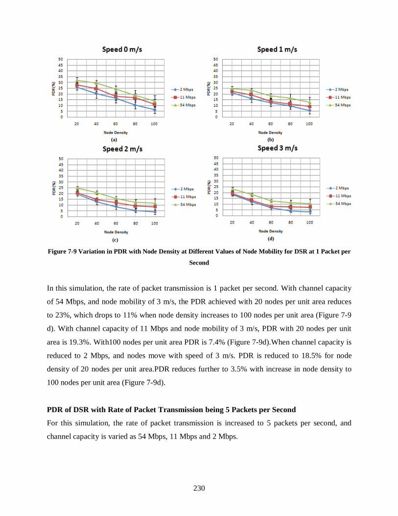
230

Figure 7-9 Variation in PDR with Node Density at Different Values of Node Mobility for DSR at 1 Packet per

Second

In this simulation, the rate of packet transmission is 1 packet per second. With channel capacity

of 54 Mbps, and node mobility of 3 m/s, the PDR achieved with 20 nodes per unit area reduces

to 23%, which drops to 11% when node density increases to 100 nodes per unit area (Figure 7-9

d). With channel capacity of 11 Mbps and node mobility of 3 m/s, PDR with 20 nodes per unit

area is 19.3%. With100 nodes per unit area PDR is 7.4% (Figure 7-9d).When channel capacity is

reduced to 2 Mbps, and nodes move with speed of 3 m/s. PDR is reduced to 18.5% for node

density of 20 nodes per unit area.PDR reduces further to 3.5% with increase in node density to

100 nodes per unit area (Figure 7-9d).

PDR of DSR with Rate of Packet Transmission being 5 Packets per Second

For this simulation, the rate of packet transmission is increased to 5 packets per second, and

channel capacity is varied as 54 Mbps, 11 Mbps and 2 Mbps.

(a) (b)

(d) (c)

231

Figure 7-10 Variation in PDR with Node Density at Different Values of Node Mobility for DSR at 5 Packets

per Second

With 54 Mbps of channel capacity, and node mobility of 3 m/s, PDR is 12% at the node density

of 20 nodes per unit area. PDR drops to 8% when node density is increased to 100 nodes per unit

area (Figure 7-10d). At the channel capacity of 11 Mbps, PDR for nodes moving at 3 m/s, with

20 nodes per unit area is 11%, and that for 100 nodes per unit area is 6.8%. Results for the same

are presented in Figure 7-10d.

As can be seen from the results of Figure 7-10d, when channel capacity is reduced to 2 Mbps,

PDR for nodes moving at a speed of 3 m/s, with 20 nodes per unit area is 8% and drops to 5%

with increase in node density to 100 nodes per unit area.


For these simulations, the rate of packet transmission is increased to 15 packets per second. At

the channel capacity of 54 Mbps, and node mobility of 3 m/s, the PDR obtained with 20 nodes

(a) (b)

(c) (d)

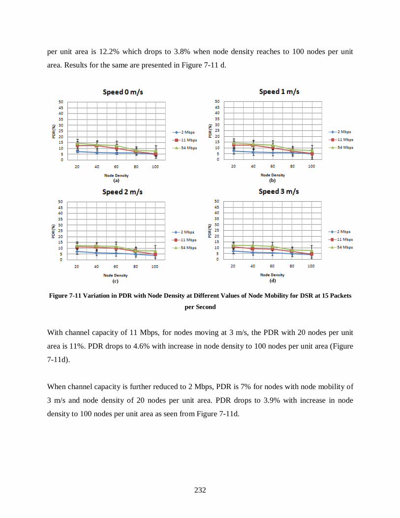
232

per unit area is 12.2% which drops to 3.8% when node density reaches to 100 nodes per unit

area. Results for the same are presented in Figure 7-11 d.


per Second

With channel capacity of 11 Mbps, for nodes moving at 3 m/s, the PDR with 20 nodes per unit

area is 11%. PDR drops to 4.6% with increase in node density to 100 nodes per unit area (Figure

7-11d).

When channel capacity is further reduced to 2 Mbps, PDR is 7% for nodes with node mobility of

3 m/s and node density of 20 nodes per unit area. PDR drops to 3.9% with increase in node

density to 100 nodes per unit area as seen from Figure 7-11d.

(a) (b)

(c) (d)

233


The variation of PDR is studied by varying node density and mobility of nodes at channel

capacities of 54 Mbps, 11 Mbps and 2 Mbps. DSR is used for routing of information with

increased packet transmission rate of 25 packets per second.


per Second

For channel capacity of 54 Mbps, with node mobility of 3 m/s, PDR is 11.7% with 20 nodes per

unit area. PDR reduces to 6% when node density increases to 100 nodes per unit area. For

channel capacity of 11 Mbps, with node mobility of 3 m/s, PDR is 7.6% for 20 nodes per unit

area. PDR drops to 3.9% when node density increases to 100 nodes per unit area. Results for the

simulations are presented in Figure 7-12d.

(a)

(c) (d)

(b)

234

With channel capacity of 2 Mbps, and mobility of nodes being 3 m/s, PDR is 6.6% for 20 nodes

per unit area and it drops to 3.5% with node density of 100 nodes per unit area (Figure 7-12d).

Table 7-4 Standard Deviation with respect to Mean for DSR PDR

DSR PDR 1 Packet per Second


0 m/s 3 m/s 0 m/s 3 m/s 0 m/s 3 m/s


20 25.7 2 18.5 1.5 28 2.2 19.3 1.5 32 2.2 23.1 1.6

60 16.5 4.1 7 1.7 18 3.2 8 1.4 24.5 2.7 13 1.4

100 6.4 3 3.5 1.7 11.2 4.3 7.4 2.8 13.9 4.8 10.7 3.7

DSR PDR 25 Packets per Second


0 m/s 3 m/s 0 m/s 3 m/s 0 m/s 3 m/s


20 7.4 2.8 6.9 2.5 8.6 2.5 7.6 2.2 13.4 2.7 11.7 2.4

60 7 2.5 7 2.8 8 2.5 7.5 2.3 12.4 3.1 11 2.7

100 4 3.2 3.6 3.2 4.6 3.2 3.9 2.7 7.2 5.2 6.5 4.7

Values of Standard Deviation (SD) with respect to Mean (M) for DSR PDR are presented in

Table 7-4. To keep the length of the table concise, these values are presented only selected

parameters, as discussed in Section 7.2.1. The Mean (M) denotes the values of PDR (%), plotted

in the results presented in Figure 7-9 (for rate of 1 Packet per Second) and Figure 7-12 (for rate

of 25 Packets per Second).

From the variation in PDR with node density and mobility, at different rates of packet

transmission, following conclusions can be drawn:

1. PDR deteriorates with increase in node density for all the values of channel capacity.

This is because DSR makes use of omnidirectional antenna for communication, due to

which nodes experience exposed node problem. This problem gets aggravated with

increase in node density. Number of communicating nodes also increases with increase in

235

node density. As a consequence, contention between nodes to access the medium also

increases, leading to delays over multihop communication

2. PDR drops when channel capacity is reduced. This is expected, because with drop in

channel capacity, ability of the channel to handle network traffic reduces, leading to

deterioration in network performance

3. Mobility of nodes also induces drop in PDR at all values of channel capacity. However,

since DSR is also a multipath routing protocol, availability of backup routes in case of

route breakages ensures that the drop in PDR is not drastic across different values of

mobility of nodes

4. PDR drops with increase in rate of packet transmission. This is because unlike DPDA-

MRP, DSR uses single polarisation with omnidirectional antenna. In DSR, with single

polarisation, there is no provision of simultaneous communication over orthogonal

polarisations. With use of omnidirectional antenna, nodes experience the problem of

exposed nodes. When the rate of packet transmission increases, congestion of network

increases, leading to reduced PDR

5. From the values presented in Table 7-4 it is observed that standard deviation increases

with increase in node density. This trend is same as that observed for DPDA-MRP, and it

is discussed in detail in Section 7.2.1.

7.3 Effect of Variation in Density and Mobility of Nodes on Throughput Achieved by

DPDA-MRP, SPDA-MRP and DSR with Varying Rate of Packet Transmission

Throughput is an essential parameter used to evaluate the performance of a network. In the

simulations, throughput is computed as the number of bits received successfully by the

destination node over the duration of simulation.

In this section the throughput achieved by DPDA-MRP, SPDA-MRP and DSR is studied. For

this study, the network scenarios are developed based on the scenario specifications given in

Table 7-1. Simulations are carried out for different values of density and mobility of nodes. Rate

236

of packet transmission is varied to study the performance of the network when different routing

protocols are used for communication. Capacity of the communication channel is also varied to

study how different routing protocols perform with change in capacity of the communication

channel.

7.3.1 Analysis of Variation in Throughput of DPDA-MRP

In this section, variation in throughput of the network is studied when DPDA-MRP is used for

routing of information. The throughput is determined for packet transmission rates of 1, 5, 15

and 25 packets per second.

The performance is analysed for density of nodes varied from 20 nodes per unit area to 100

nodes per unit area, in steps of 20. Mobility of nodes is varied from 0 m/s (stationary nodes), to 3

m/s in steps of 1, to simulate the walking and running speed of humans. The performance of

DPDA-MRP is studied at channel capacities of 2 Mbps, 11 Mbps and 54 Mbps.

Throughput of DPDA-MRP with Rate of Packet Transmission being 1 Packet per Second

The variation in network throughput achieved by the use of DPDA-MRP is studied when the rate

of packet transmission is 1 packet per second. The variation in obtained throughput of DPDA-

MRP, with varying node density and mobility of nodes is presented in Figure 7-13.With nodes

moving at speed of3 m/s and communicating over a channel of 54 Mbps capacity, throughput is

23 kbps at node density of 20 nodes per unit area.

When node density increases to 100 nodes per unit area, the corresponding throughput is 166

kbps (Figure 7-13d).

At the channel capacity of 11 Mbps, the throughput increases from 20 kbps to 150 kbps with

increase in node density of 20 nodes to 100 nodes per unit area.

However, at the channel capacity of 2 Mbps, the increase in throughput with node density is not

significant, as it increases from 12.4 kbps to 39.4 kbps when node density changes from 20 to

100 nodes per unit area (Figure 7-13d).

237


MRP at1 Packet per Second

Throughput of DPDA-MRP with Rate of Packet Transmission being 5 Packets per Second

The variation in the throughput achieved when DPDA-MRP is used as the routing protocol for

communication is studied at different values of density and mobility of nodes. Capacities of

communication channel used for this study are 54 Mbps, 11 Mbps and 2 Mbps. The simulation

results are presented in Figure 7-14.

For the channel capacity of 54 Mbps, network throughput increases with increase in node density

of up to 80 nodes per unit area and then deteriorates when node density is further increased to

100 nodes per unit area. As seen from Figure 7-14d, when nodes move at 3 m/s, throughput with

20 nodes per unit area is 136.8 kbps. It increases to 521.7 kbps with 80 nodes per unit area.

Throughput drops to 351.1 kbps when node density is further increased to 100 nodes per unit

area. At 11 Mbps, when nodes move at 3 m/s, the achieved throughput with 20 nodes per unit

(a) (b)

(c) (d)

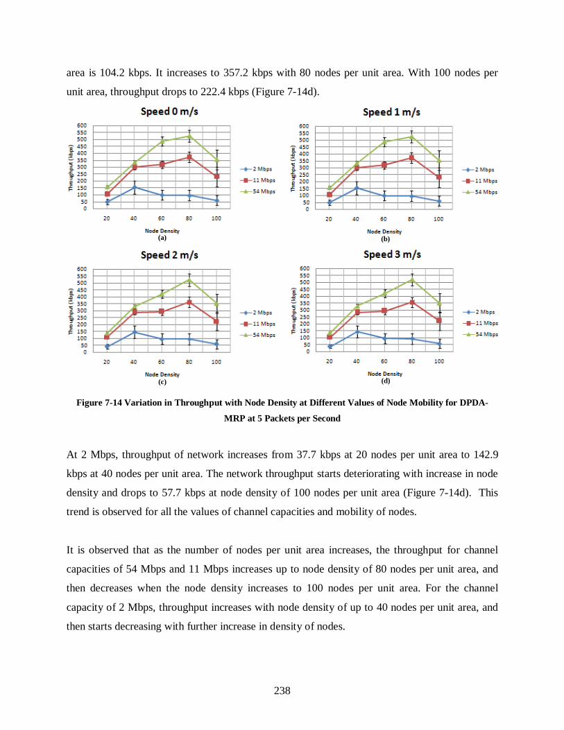
238

area is 104.2 kbps. It increases to 357.2 kbps with 80 nodes per unit area. With 100 nodes per

unit area, throughput drops to 222.4 kbps (Figure 7-14d).


MRP at 5 Packets per Second

At 2 Mbps, throughput of network increases from 37.7 kbps at 20 nodes per unit area to 142.9

kbps at 40 nodes per unit area. The network throughput starts deteriorating with increase in node

density and drops to 57.7 kbps at node density of 100 nodes per unit area (Figure 7-14d). This

trend is observed for all the values of channel capacities and mobility of nodes.

It is observed that as the number of nodes per unit area increases, the throughput for channel

capacities of 54 Mbps and 11 Mbps increases up to node density of 80 nodes per unit area, and

then decreases when the node density increases to 100 nodes per unit area. For the channel

capacity of 2 Mbps, throughput increases with node density of up to 40 nodes per unit area, and

then starts decreasing with further increase in density of nodes.

(c)

(a)

(d)

(b)

239


The rate of packet transmission is increased to 15 packets per second to study its effect on the

throughput when DPDA-MRP is used for communication. The variation in network throughput

obtained by using DPDA-MRP for routing of information at different values of channel capacity

and mobility of nodes is presented in Figure 7-15.



With channel capacity of 54 Mbps, when nodes move at 3 m/s, network throughput increases

from 231.4 kbps with 20 nodes per unit area to 437.2 kbps with 60 nodes per unit area.

Throughput degrades to 271.6 kbps with 100 nodes per unit area (Figure 7-15d). When the

channel capacity is reduced to 11 Mbps, keeping mobility of nodes as same, throughput with

node density of 20 nodes per unit area is 176.4 kbps. It increases to 269.3 kbps when node

density is 60 nodes per unit area and reduces to 153 kbps with increase in node density to 100

nodes per unit area (Figure 7-15d). At the channel capacity of 2 Mbps, with the nodes moving at

3 m/s, throughput with 20 nodes per unit area is 53 kbps. It increases to 99.6 kbps when density

(d) (c)

(b) (a)

240

of nodes is changed to 40 nodes per unit area (Figure 7-15d). Throughput drops to 37.4 kbps

when density of nodes is further increased to 100 nodes per unit area.


In this scenario, the variation in network throughput achieved through DPDA-MRP is studied

when the rate of packet transmission is increased to 25 packets per second. The variation in

network throughput is analysed for varying density and mobility of nodes over different values

of channel capacity. The results are presented in Figure 7-16.



At channel capacity of 54 Mbps and node mobility of 3 m/s, throughput with 20 nodes per unit

area is 218.6 kbps. It increases to 396 kbps for a node density is 60 nodes per unit area (Figure

7-16 d). Throughput drops to 244.8 kbps when node density is increased to 100 nodes per unit

area. At 11 Mbps, with node mobility of 3 m/s, throughput is 178.5 kbps with 20 nodes per unit

area. Throughput increases to 246.1 kbps at 60 nodes per unit area. With further increase in node

(a) (b)

(c) (d)

241

density, throughput starts to degrade and drops to 140.4 kbps with node density of 100 nodes per

unit area (Figure 7-16 d). Throughput achieved with channel capacity of 2 Mbps is the least and

it constantly deteriorates with increase in density and mobility of nodes. When node mobility is 3

m/s, throughput with 20 nodes per unit area is 87.5 kbps which further deteriorates to 33.4 kbps

when node density is changed to 100 nodes per unit area (Figure 7-16 d).

Table 7-5 Standard Deviation with respect to Mean for DPDA-MRP Throughput

DPDA-MRP Throughput 1 Packet per Second


0 m/s 3 m/s 0 m/s 3 m/s 0 m/s 3 m/s


20 15 3.7 12.4 3.8 20.1 0.9 10.8 1 22.4 1 23 1

60 25 6.6 27.4 7.2 106 3.4 101 .32 107 3.4 102 3.2

100 43.4 11.1 39.4 10 150 15 150 15 167 10 166 10

DPDA-MRP Throughput 25 Packets per Second


0 m/s 3 m/s 0 m/s 3 m/s 0 m/s 3 m/s


20 104 32 87.6 26.9 184 37.2 179 36.2 248 25.3 219 22.3

60 92 41.5 63.4 28.7 261 58 246 54.6 439 52.2 396 47.1

100 51 47.2 33.4 31 145 67.7 140 65.4 258 80.6 245 76.4

Values of Standard Deviation (SD) with respect to Mean (M) for DPDA-MRP Throughput are


selected parameters, as discussed in Section 7.2.1. The Mean (M) denotes the values of

throughput in kbps, plotted in the results presented in Figure 7-13 (for rate of 1 Packet per

Second) and Figure 7-16 (for rate of 25 Packets per Second). The results for variation in

throughput when DPDA-MRP is used for routing of information at different rates of packet

transmission are presented in Figure 7-13 to Figure 7-16, and Table 7-5. Following inferences

can be drawn from obtained results

1. The increase of throughput with increase in node density is expected because of the

increase in number of transmitting nodes infusing packets into the channel. However,

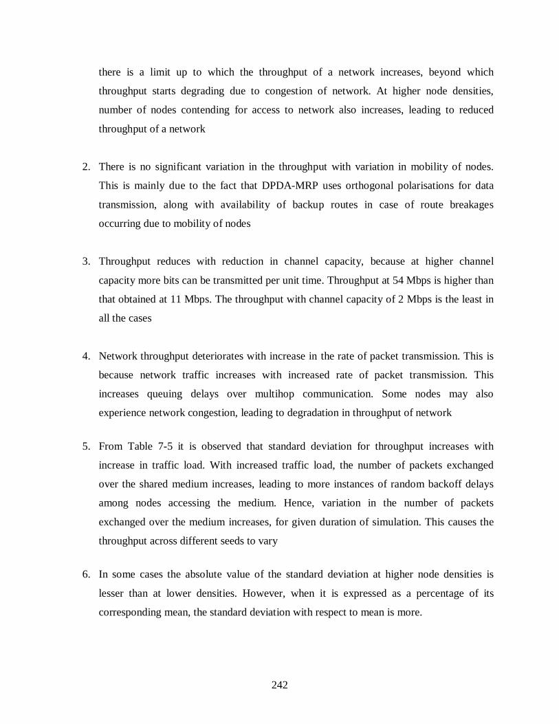
242

there is a limit up to which the throughput of a network increases, beyond which

throughput starts degrading due to congestion of network. At higher node densities,

number of nodes contending for access to network also increases, leading to reduced

throughput of a network

2. There is no significant variation in the throughput with variation in mobility of nodes.

This is mainly due to the fact that DPDA-MRP uses orthogonal polarisations for data

transmission, along with availability of backup routes in case of route breakages

occurring due to mobility of nodes

3. Throughput reduces with reduction in channel capacity, because at higher channel

capacity more bits can be transmitted per unit time. Throughput at 54 Mbps is higher than

that obtained at 11 Mbps. The throughput with channel capacity of 2 Mbps is the least in

all the cases

4. Network throughput deteriorates with increase in the rate of packet transmission. This is

because network traffic increases with increased rate of packet transmission. This

increases queuing delays over multihop communication. Some nodes may also

experience network congestion, leading to degradation in throughput of network

5. From Table 7-5 it is observed that standard deviation for throughput increases with

increase in traffic load. With increased traffic load, the number of packets exchanged

over the shared medium increases, leading to more instances of random backoff delays

among nodes accessing the medium. Hence, variation in the number of packets

exchanged over the medium increases, for given duration of simulation. This causes the

throughput across different seeds to vary

6. In some cases the absolute value of the standard deviation at higher node densities is

lesser than at lower densities. However, when it is expressed as a percentage of its

corresponding mean, the standard deviation with respect to mean is more.

243

7.3.2 Analysis of Variation in Throughput of SPDA-MRP

This section presents the variation in throughput realised through SPDA-MRP for routing of

information. Variation of throughput is studied for different rates of packet transmission, with

increase in density and mobility of nodes. The variation in throughput is analysed over channel

capacities of 54 Mbps, 11 Mbps and 2 Mbps.

Throughput of SPDA-MRP with Rate of Packet Transmission being 1 Packet per Second

The variation in throughput of SPDA-MRP with increase in density of nodes is presented in

Figure 7-17. The results are obtained for different values of node mobility.

Figure 7-17 Variation in Throughput with Node Density at Different Values of Node Mobility for SPDA-MRP

at 1 Packet per Second

At the channel capacity of 54 Mbps, when nodes move at 3 m/s, the throughput with 20 nodes

per unit area is 25.4 kbps. It increases to 79 kbps with 60 nodes per unit area.

(a) (b)

(c) (d)

244

It then drops to 37.7 kbps when node density is further increased to 100 nodes per unit area

(Figure 7-17d). With channel capacity of 11 Mbps, and node mobility of 3 m/s, throughput with

20 nodes per unit area is 19.4 kbps. It increases to 72.8 kbps with increase in node density to 60

nodes per unit area. With further increase in node density to 100 nodes per unit area, the

throughput drops to 32.5 kbps (Figure 7-17d). Reducing the channel capacity to 2 Mbps leads to

degradation in throughput of the network. Configuring the mobility of node as 3 m/s, the PDR

with 20 nodes per unit area is 9.5 kbps. It increases to 20.8 kbps with increase in node density to

60 nodes per unit area. With further increase in node density to 100 nodes per unit area,

throughput drops to 10.7 kbps (Figure 7-17d).

Throughput of SPDA-MRP with Rate of Packet Transmission being 5 Packets per Second

The effect of increasing the rate of packet transmission to 5 packets per second on throughput of

the network is studied with increase in node density.



(b) (a)

(c) (d)

245

Simulated results for the performance of the network in terms of throughput are presented in

Figure 7-18 for different values of node mobility. At the channel capacity of 54 Mbps,

throughput initially increases with increase in node density, and then deteriorates when node

density is increased further. This trend is observed for all the values of mobility of nodes (Figure

7-18a, b, c and d).

When nodes move at 3 m/s, the throughput with node density of 20 nodes per unit area, is 118

kbps. It increases to 124 kbps when node density increases to 40 nodes per unit area. Throughput

deteriorates to 57 kbps when node density is further increased to 100 nodes per unit area. Similar

trend is observed when channel capacity is reduced to 11 Mbps.

With node mobility of 3 m/s, throughput with 20 nodes per unit area is 108.4 kbps, which

increases to 119.6 kbps with increase in node density to 40 nodes per unit area. Throughput

deteriorates with further increase in node density. When node density increases to 100 nodes per

unit area, throughput drops to 38.3 kbps (Figure 7-18d).

When channel capacity is reduced to 2 Mbps, throughput of the network deteriorates drastically

with increase in node density. A similar trend is observed for all values of mobility of nodes.

With node mobility of 3 m/s, throughput with 20 nodes per unit area is 95.4 kbps. It drops to 14

kbps when node density increases to 100 nodes per unit area (Figure 7-18d).


The rate of packet transmission is increased further to 15 packets per second to study its effect on

the performance of SPDA-MRP. The results for variation in throughput with increase in density

and mobility of nodes are presented in Figure 7-19.

At 54 Mbps, throughput initially increases with increase in node density and then starts to

deteriorate when node density is increased further. This trend is observed for all the values of

mobility of nodes (Figure 7-19a, b, c and d). With node mobility of 3 m/s, for 20 nodes per unit

area the throughput is 97.1 kbps and it increases to 105.8 kbps with node density of 40 nodes per

246

unit area. With further increase in node density, throughput starts to deteriorate. Throughput with

100 nodes per unit area drops to 49.3 kbps (Figure 7-19d).



At channel capacity of 11 Mbps, at lower values of node mobility (0 m/s and 1 m/s), throughput

increases up to node density of 40 nodes per unit area. It then deteriorates when node density is

increased further (Figure 7-19a and b). However, with mobility of nodes at 2 m/s and 3 m/s,

throughput drops consistently with increase in node density (Figure 7-19c and d).

Throughput achieved with channel capacity of 2 Mbps is the least. It increases with increase in

node density of up to 40 nodes per unit area, and then drops when node density is increased

further up to 100 nodes per unit area. This trend is noticed for all values of node mobility (Figure

7-19a, b, c and d).

(a) (b)

(c) (d)

247


The effect of further increase in the rate of packet transmission to 25 packets per second on

network throughput when SPDA-MRP is used for routing is also analysed. The results for

variation in network throughput with increase in node density over different values of node

mobility are presented in Figure 7-20.



Throughput with rate of packet transmission being 25 packets per second is lesser when

compared to that achieved when the rate of packet transmission is 15 packets per second. This

degradation in throughput with increase in the rate of packet transmission is observed for all

values of channel capacity (Figure 7-20a, b, c and d).

At 54 Mbps, throughput increases with increase in node density of up to 60 nodes per unit area.

With further increase in node density, throughput starts to deteriorate. This trend is observed for

all the values of mobility of nodes (Figure 7-20a, b, c and d). Throughput reduces with reduction

(a) (b)

(c) (d)

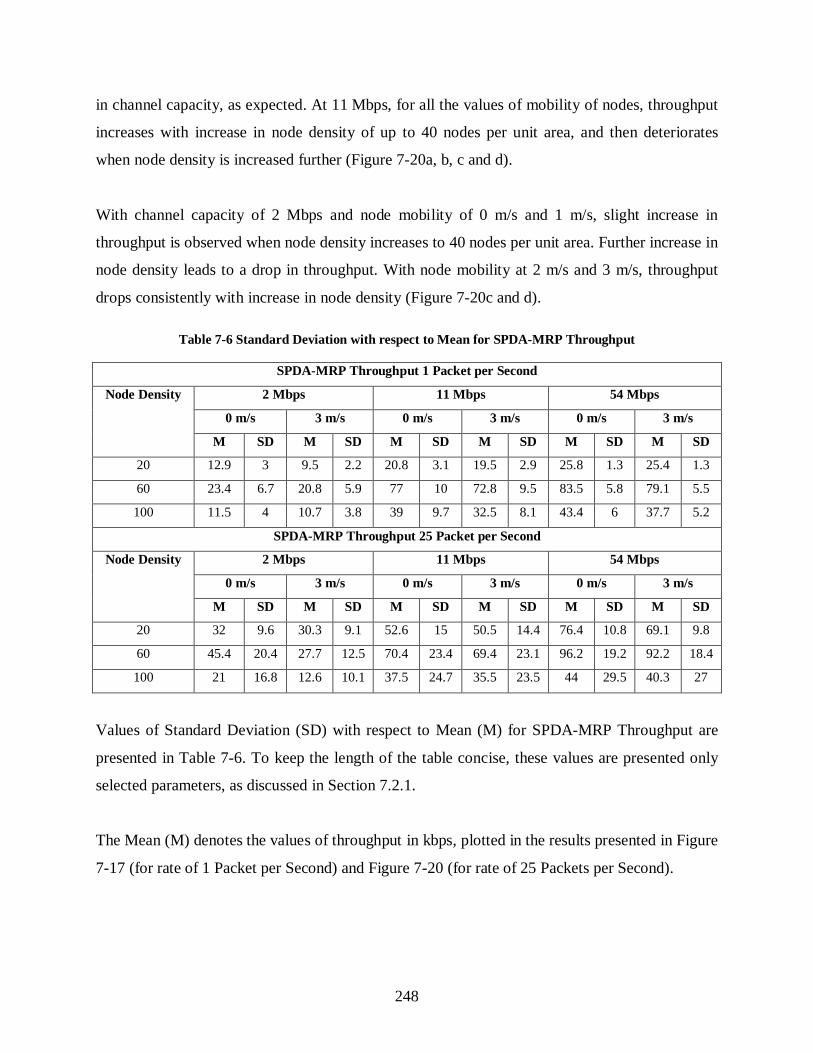
248

in channel capacity, as expected. At 11 Mbps, for all the values of mobility of nodes, throughput

increases with increase in node density of up to 40 nodes per unit area, and then deteriorates

when node density is increased further (Figure 7-20a, b, c and d).

With channel capacity of 2 Mbps and node mobility of 0 m/s and 1 m/s, slight increase in

throughput is observed when node density increases to 40 nodes per unit area. Further increase in

node density leads to a drop in throughput. With node mobility at 2 m/s and 3 m/s, throughput

drops consistently with increase in node density (Figure 7-20c and d).

Table 7-6 Standard Deviation with respect to Mean for SPDA-MRP Throughput

SPDA-MRP Throughput 1 Packet per Second


0 m/s 3 m/s 0 m/s 3 m/s 0 m/s 3 m/s


20 12.9 3 9.5 2.2 20.8 3.1 19.5 2.9 25.8 1.3 25.4 1.3

60 23.4 6.7 20.8 5.9 77 10 72.8 9.5 83.5 5.8 79.1 5.5

100 11.5 4 10.7 3.8 39 9.7 32.5 8.1 43.4 6 37.7 5.2

SPDA-MRP Throughput 25 Packet per Second


0 m/s 3 m/s 0 m/s 3 m/s 0 m/s 3 m/s


20 32 9.6 30.3 9.1 52.6 15 50.5 14.4 76.4 10.8 69.1 9.8

60 45.4 20.4 27.7 12.5 70.4 23.4 69.4 23.1 96.2 19.2 92.2 18.4

100 21 16.8 12.6 10.1 37.5 24.7 35.5 23.5 44 29.5 40.3 27

Values of Standard Deviation (SD) with respect to Mean (M) for SPDA-MRP Throughput are


selected parameters, as discussed in Section 7.2.1.

The Mean (M) denotes the values of throughput in kbps, plotted in the results presented in Figure

7-17 (for rate of 1 Packet per Second) and Figure 7-20 (for rate of 25 Packets per Second).

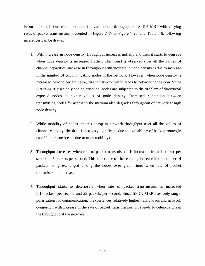
249

From the simulation results obtained for variation in throughput of SPDA-MRP with varying

rates of packet transmission presented in Figure 7-17 to Figure 7-20, and Table 7-6, following

inferences can be drawn:

1. With increase in node density, throughput increases initially and then it starts to degrade

when node density is increased further. This trend is observed over all the values of

channel capacities. Increase in throughput with increase in node density is due to increase

in the number of communicating nodes in the network. However, when node density is

increased beyond certain value, rise in network traffic leads to network congestion. Since

SPDA-MRP uses only one polarisation, nodes are subjected to the problem of directional

exposed nodes at higher values of node density. Increased contention between

transmitting nodes for access to the medium also degrades throughput of network at high

node density

2. While mobility of nodes induces adrop in network throughput over all the values of

channel capacity, the drop is not very significant due to availability of backup routes(in

case if one route breaks due to node mobility)

3. Throughput increases when rate of packet transmission is increased from 1 packet per

second to 5 packets per second. This is because of the resulting increase in the number of

packets being exchanged among the nodes over given time, when rate of packet

transmission is increased

4. Throughput starts to deteriorate when rate of packet transmission is increased

to15packets per second and 25 packets per second. Since SPDA-MRP uses only single

polarisation for communication, it experiences relatively higher traffic loads and network

congestion with increase in the rate of packet transmission. This leads to deterioration in

the throughput of the network

250

5. From values of standard deviation presented in Table 7-6 it is seen that standard deviation

increases with increase in node density. This trend is same as that observed in DPDA-

MRP, and it is discussed in detail in Section 7.3.1.

7.3.3 Analysis of Variation in Throughput of DSR

DSR is a multipath routing protocol which uses omnidirectional antenna and single polarisation

for communication. Performance analysis of DSR is carried out for different rates of packet

transmission, with varying values of density and mobility of nodes. Simulations are carried out

for channel capacities of 54 Mbps, 11 Mbps and 2 Mbps.

Throughput of DSR with Rate of Packet Transmission being 1 Packet per Second

In this set of simulations, DSR is used as the routing protocol for multihop communication

among the nodes. The variation in throughput with different values of node density and mobility

of nodes is presented in Figure 7-21.

Figure 7-21 Variation in Throughput with Node Density at Different Values of Node Mobility for DSR at 1

Packet per Second

(a) (b)

(c) (d)

251

From the simulation results depicted in Figure 7-21, it is observed that throughput deteriorates

with increase in node density for all values of node mobility (Figure 7-21a, b, c and d). Slight

degradation in throughput is observed with increase in node mobility (Figure 7-21a, b, c and d).

Similar response is observed for all the values of channel capacity.

Throughput of DSR with Rate of Packet Transmission being 5 Packets per Second

The effect of increase in rate of packet transmission to 5 packets per second on the throughput of

the network achieved with DSR is studied. The variation in throughput with variation in density

and mobility of nodes for different values of channel capacity is presented in Figure 7-22. From

the simulation results depicted in Figure 7-22, it is observed that throughput achieved with

transmission rate of 5 packets per second is higher than that achieved with transmission rate of 1

packet per second, for all values of mobility of nodes.


Packets per Second

(a) (b)

(c) (d)

252

Throughput reduces with increase in node density. There is slight deterioration in the throughput

with increase in mobility of nodes (Figure 7-22a, b, c and d). These observations hold true for all

values of channel capacity.


The rate of packet transmission is increased to 15 packets per second to study its effect on

network throughput, when DSR is used as the routing protocol. The variation in throughput with

varying values of density and mobility of nodes, at channel capacities of 54 Mbps, 11 Mbps and

2 Mbps is presented in Figure 7-23.


Packets per Second

From the simulation results illustrated in Figure 7-23a, b, c and d. It is observed that for all the

values of channel capacities throughput degrades with increase in node density and mobility of

(a) (b)

(c) (d)

253

nodes. Throughput at the transmission rate of 15 packets per second is lesser than that with the

transmission rate of 5 packets per second for all values of channel capacities.


Rate of packet transmission is further increased to 25 packets per second to study its effect on

network throughput obtained with DSR as the routing protocol. The variation in throughput with

increase in density and mobility of nodes for different values of channel capacity is presented in

Figure 7-24.


Packets per Second

Values of Standard Deviation (SD) with respect to Mean (M) for DSR Throughput are presented

in Table 7-7. To keep the length of the table concise, these values are presented only selected

parameters, as discussed in Section 7.2.1. The Mean (M) denotes the values of throughput in

kbps, plotted in the results presented in Figure 7-21 (for rate of 1 Packet per Second) and Figure

7-24 (for rate of 25 Packets per Second).

(a) (b)

(c) (d)

254

Table 7-7 Standard Deviation with respect to Mean for DSR Throughput

DSR Throughput 1 Packet per Second


0 m/s 3 m/s 0 m/s 3 m/s 0 m/s 3 m/s


20 4.1 1 2.3 0.57 6 1.3 6 1.3 8.7 1.2 7.8 1.1

60 2 0.9 1.2 0.55 3 1.3 2.8 1.2 4.5 1.8 5.6 2.1

100 1 0.7 1 0.75 2 1.4 1.9 1.7 3.1 1.9 2.9 2.4

DSR Throughput 25 Packets per Second


0 m/s 3 m/s 0 m/s 3 m/s 0 m/s 3 m/s


20 4 2.1 3.7 2 9.6 4.6 5.8 2.7 12.5 3.9 12.1 3.7

60 3.5 2.5 3.1 2.1 7.6 5 5 3.3 10.9 6.2 9.3 5.4

100 1.2 1.1 1 0.9 2.7 2.4 2 1.8 7.7 5.6 3.2 3.2

From the simulation results presented in Figure 7-21 to Figure 7-24, and Table 7-7, following

inferences can be drawn about the variation in throughput of the network obtained with DSR:

1. Throughput increases when the rate of packet transmission increases from 1 packet per

second to 5 packets per second. It then drops when the rate of packet transmission is

increased further to 15 and 25 packets per second. The increase in throughput with

increase in rate of packet transmission is due to increase in the number of packets

transmitted per unit time. However, when rate of packet transmission is increased further,

nodes experience congestion in the network due to increase in traffic. This leads to

queuing delays, leading to drop in throughput over multihop communication

2. It is observed that throughput drops with increase in node density for all the values of

channel capacity. With increase in node density, number of communicating nodes also

increases, leading to increase in contention among the transmitting nodes for access to the

medium. The problem of exposed nodes is experienced due to omnidirectional

communication by DSR protocol. The severity of the problem of exposed nodes increases

255

with increased density of nodes, which in turn leads to drop in throughout of the network

over multihop communication

3. Though mobility of nodes induces drop in throughput, the drop is not very severe due to

the availability of multiple alternate routes. In DSR, when throughput reaches minimum

achievable throughput, it does not drop further as throughput has already reached the

minimum possible throughput of 1 kbps

4. Throughput decreases with decrease in channel capacity, as expected.

5. From values presented in Table 7-7it is observed that standard deviation increases with

increase in node density. This trend is same as that observed in DPDA-MRP, and it is

discussed in detail in Section 7.3.1.

7.4 Comparison of PDR Achieved with DPDA-MRP, SPDA-MRP and DSR with Node

Density of 100 Nodes per Unit Area

In Sections 7.2 and 7.3, performance analysis of the three protocols namely DPDA-MRP, SPDA-

MRP and DSR was presented. The focus of these sections was on the individual performance of

the three protocols. This section presents a comparison of the performance of three routing

protocols in terms of PDR, when the node density is 100 nodes per unit area.

At 100 nodes per unit area, the number of nodes trying to access the medium is highest.

Therefore, it becomes important to study the difference in the performance of the three routing

protocols when more nodes try to access the medium at the same time.

The comparison is presented for rates of packet transmission of 1, 5, 15 and 25 packets per

second. Comparison in the performance of the routing protocols is carried out for channel

capacities of 54 Mbps, 11 Mbps and 2 Mbps. The aim of this study is to distinguish between the

capabilities of the three routing protocols in responding to the variation in packet rates.

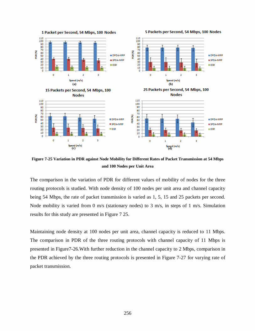
256

Figure 7-25 Variation in PDR against Node Mobility for Different Rates of Packet Transmission at 54 Mbps

and 100 Nodes per Unit Area

The comparison in the variation of PDR for different values of mobility of nodes for the three

routing protocols is studied. With node density of 100 nodes per unit area and channel capacity

being 54 Mbps, the rate of packet transmission is varied as 1, 5, 15 and 25 packets per second.

Node mobility is varied from 0 m/s (stationary nodes) to 3 m/s, in steps of 1 m/s. Simulation

results for this study are presented in Figure 7 25.

Maintaining node density at 100 nodes per unit area, channel capacity is reduced to 11 Mbps.

The comparison in PDR of the three routing protocols with channel capacity of 11 Mbps is

presented in Figure7-26.With further reduction in the channel capacity to 2 Mbps, comparison in

the PDR achieved by the three routing protocols is presented in Figure 7-27 for varying rate of

packet transmission.

(a)

(c)

(b)

(d)

257

Figure 7-26 Variation in PDR against Node Mobility for Different Rates of Packet Transmission at 11Mbps


From the results illustrated in Figure 7-25, Figure7-26 and Figure 7-27, following inferences can

be drawn

1. The PDR achieved by DPDA-MRP protocol is the highest among all the three routing

protocols. In DPDA-MRP orthogonal polarisations are used simultaneously for

directional communication. Transmission over each polarisation can be considered as a

separate channel. Simultaneous use of orthogonal channels for directional communication

also avoids directional exposed node problem, leading to high PDR

2. PDR achieved by SPDA-MRP is lesser than that of DPDA-MRP and greater than that of

DSR. SPDA-MRP uses only one polarisation for directional communication. Availability

of single polarisation channel also leads to directional exposed node problem, leading to

(a) (b)

(c) (d)

258

lower PDR when compared to that achieved with DPDA-MRP. However, directional

communication reduces the instances of exposed node problem when compared

omnidirectional communication. Therefore, SPDA-MRP achieves higher PDR than DSR

3. PDR of DSR is the least when compared to that of DPDA-MRP and SPDA-MRP. DSR

carries out omnidirectional communication over single polarisation, due to which nodes

experience exposed node problem, leading to reduced PDR.

4. PDR reduces with increase in the rate of packet transmission for all the three routing

protocols. With increase in the rate of packet transmission, traffic on the network

increases leading to queuing delays over multihop communication and network

congestion. This leads to drop in PDR with increase in rate of packet transmission

Figure 7-27 Variation in PDR against Node Mobility for Different Rates of Packet Transmission at 2 Mbps


(a) (b)

(c) (d)

259

5. While PDR drops with increase in node mobility for all the three routing protocols, the

drop is not significant. Higher the mobility of the nodes, greater are the chances of route

breakage. Breakage of routes can lead to drop in packets. Packets need to be stored at the

transmitting nodes till new routes are established. This leads to drop in PDR with

increase in mobility of nodes. However, this drop is not significant for any of the three

protocols since all the three are multipath routing protocols and maintain backup routes in

case one route breaks

6. PDR decreases with reduction in the capacity of channel. When capacity of the channel is

reduced, the ability of the channel to handle network traffic diminishes, leading to

degradation in performance

7.5 Comparison of Throughput Achieved with DPDA-MRP, SPDA-MRP and DSR with

Node Density of 100 Nodes per Unit Area

This section compares the throughput achieved through DPDA-MRP, SPDA-MRP and DSR

protocols with varying mobility of nodes and rates of packet transmission.



(a) (b)

(c) (d)

260

The comparison in the performance of these routing protocols is carried out over channels

capacities of 54 Mbps, 11 Mbps and 2 Mbps. Variation in throughput is studied for packet

transmission rates of 1, 5, 15 and 25 packets per second.



The results for comparison of throughput obtained with the three routing protocols when

capacity of the channel is 54 Mbps at different rates of packet transmission are presented in

Figure 7-28.

The difference in throughput of DPDA-MRP, SPDA-MRP and DSR, with different values of

mobility of nodes and rates of packet transmission, when capacity of the channel is reduced to 11

Mbps is presented in Figure 7-29. The difference in throughput of the three routing protocols,

when capacity of the channel is further reduced to 2 Mbps at different rates of packet

transmission and mobility of nodes is presented in Figure 7-30.

(a) (b)

(c) (d)

261



From the results presented in Figure 7-28, Figure 7-29 and Figure 7-30, following inferences can

be drawn

1. Throughput increases initially with increase in the rate of packet transmission up to 5

packets per second. It then reduces when the rate of packet transmission is further

increased to 15 and 25 packets per second. This trend is observed for all the three routing

protocols. Initially, when the rate of packet transmission is increased, network throughput

increases. This is because of the increase in the number of packets transmitted per unit

time. However, when the rate of packet transmission is increased further, nodes

experience congestion of network, leading to drop in throughput of network

2. Throughput of DPDA-MRP is the highest among all the routing protocols. DPDA-MRP

uses two orthogonal polarisations simultaneously for communication. It also mitigates the

(a) (b)

(c) (d)

262

problem of interference, exposed nodes and directional exposed nodes leading to high

network throughput

3. Throughput of SPDA-MRP is lesser than that of DPDA-MRP and higher than that of

DSR. Since SPDA-MRP uses directional antenna for communication, the number of

nodes undergoing exposed node problem reduces at high node density. However, it uses

only one polarisation for communication. SPDA-MRP cannot prevent nodes from

undergoing the problem of directional exposed node. Instances of nodes experiencing the

directional exposed node problem increases at higher values of node density. Also, with

only one polarisation available for communication, throughput achieved by SPDA-MRP

is lesser than that of DPDA-MRP

4. Throughput of DSR is the least among the three routing protocols. DSR uses

omnidirectional communication over single polarisation. Due to this, at high node density

more nodes experience the problem of exposed nodes. With availability of only one

polarisation, throughput of DSR is lesser than that of DPDA-MRP, which has provision

of using orthogonal polarisations simultaneously for communication

5. Slight decrease in throughput is observed with increase in mobility of nodes for all the

three routing protocols. However, all the routing protocols support multipath routing. The

availability of backup routes avoids significant deterioration in performance in case

established route breaks

6. When channel capacity reduces, throughput reduces for all the three routing protocols.

This is expected, because when capacity of the channel is reduced, its ability to handle

network traffic also reduces, leading to deterioration in performance of the network

7.6 Comparison of Throughput Achieved by DPDA-MRP and SPDA-MRP

This section presents the comparison in the performance of DPDA-MRP and SPDA-MRP with

varying node density. These two protocols are chosen for comparison because this thesis

emphasises directional communication with dual polarisation.

263

Node density plays an important role in network performance because available channel

resources are shared among multiple nodes in the network. Therefore, it is essential to study the

effect of variation in node density on the performance of DPDA-MRP and SPDA-MRP routing

protocols. Since the proposed protocol is meant for MANETs, effect of mobility of nodes on the

performance of network also needs to be studied.

Figure 7-31 Comparison of Throughput Achieved by DPDA-MRP and SPDA-MRP for Varying Node Density

at Different Rates of Packet Transmission

The results presented in this section compare the performance of DPDA-MRP and SPDA-MRP

at node mobility of 0 m/s (stationary nodes) and 3 m/s. Throughput is an integral performance

parameter for any protocol. Therefore, in this section the comparison of performance of DPDA-

MRP and SPDA-MRP is carried out in terms of throughput. Channel capacity also plays an

important role in performance of a network. This study considers the channel capacity of 54

Mbps. Rate of packet transmission affects network performance as high rate of packet

transmission can lead to network congestion. Therefore, it is essential to identify appropriate rate

of packet transmission for given values of node density, channel capacity and mobility of nodes.

(a) (b)

(c) (d)

264

Results presented in Figure 7-31 compare the throughput of DPDA-MRP and SPDA-MRP for

different values of node density. The values of mobility of nodes considered for this study are 0

m/s (stationary nodes) and 3 m/s. Nodes communicate over channel with a capacity of 54 Mbps.

The comparison in throughput of DPDA-MRP and SPDA-MRP with stationary nodes (0 m/s) is

shown in Figure 7-31a and Figure 7-31b. The throughput obtained with DPDA-MRP and SPDA-

MRP with nodes moving at 3 m/s is shown in Figure 7-31c and Figure 7-31d. From the results

presented in Figure 7-31a, b, c and d, it is clear that throughput achieved by DPDA-MRP, which

uses orthogonal polarisations for simultaneous directional communication is higher than that

achieved by SPDA-MRP, which uses only one polarisation for directional communication. This

difference in performance becomes more apparent when rate of packet transmission is 5, 15 and

25 packets per second. When rate of packet transmission is 1 packet per second, throughput

achieved by DPDA-MRP is higher than that of SPDA-MRP at node density of 60, 80 and 100

nodes per unit area. This shows that DPDA-MRP is capable of better throughput than SPDA-

MRP even at high density of nodes. While increase in mobility of nodes does not cause drastic

changes in the performance of either DPDA-MRP or SPDA-MRP protocol, throughput achieved

by DPDA-MRP remains higher than that achieved by SPDA-MRP for all values of rates of

packet transmission and at all values of node density, even when nodes move at 3 m/s.

7.7 Conclusion

This chapter presented the analysis of the performance of DPDA-MRP, SPDA-MRP and DSR

protocols. The performance of these three multipath routing protocols is analysed in terms of

PDR and throughput with the help of simulations. The three multipath routing protocols

considered for this study provide services for network layer. These protocols are mainly different

from each other in terms of types of antenna (physical layer parameter) and number of

polarisations used for communication. Due to this, method of accessing the medium also varies.

The corresponding MAC layer protocols for DPDA-MRP, SPDA-MRP and DSR are DPDA-

MAC, SPDA-MAC and CSMA/CA respectively. Performance of DPDA-MAC, SPDA-MAC

and CSMA/CA was analysed in Chapter 5 for different rates of packet transmission, channel

capacities, values for node mobility and node density. Same configuration parameters are used to

study and analyse the performance of DPDA-MRP, SPDA-MRP and DSR. However, unlike

MAC protocols where performance is studied over single hop, the performance of routing

protocols is studied over multiple hops. Throughput is the principal parameter to evaluate the

265

performance of any protocol. Due to the presence of intermediate nodes facilitating routing of

information and mobility nodes, routes may break leading to drop of packets before these

packets can reach the destination node. From the results obtained for PDR of DPDA-MRP,

SPDA-MRP and DSR, it is observed that PDR reduces with increase in rate of packet

transmission for all the three routing protocols. This is attributed to the increase in network

congestion and queuing delays due to increase in traffic load. For channel capacity of 54 Mbps,

node density of 100 nodes per unit area, packet transmission rate of 1 packet per second and

node mobility of 3 m/s, PDR of DPDA-MRP is 60% higher than that of SPDA-MRP and 84%

higher than that of DSR. When rate of packet transmission is increased to 25 packets per second,

keeping all the parameters same, PDR obtained with DPDA-MRP in 25% higher than that of

SPDA-MRP and 38% higher than that of DSR. Throughput of the network initially increases

with increase in rate of packet transmission and then reduces when packet transmission rate is

increased further. From the obtained results it is observed that throughput increases when the rate

of packet transmission is increased from 1 packet per second to 5 packets per second. With

further increase in rate of packet transmission to 15 and 25 packets per second, throughput

deteriorates. Therefore, maximum throughput is obtained with packet transmission rate of 5

packets per second. This trend is observed for all the routing protocols and for all values of

channel capacity. The initial increase in throughput with increase in the rate of packet

transmission is due to the increase in the number of packets transmitted per unit time. However

further increase in the rate of packet transmission leads to increased traffic load on the network,

resulting in increased network congestion. This leads to drop in network throughput. With 5

packets transmitted per unit time, channel capacity of 54 Mbps, node density of 100 nodes per

unit area and mobility of nodes as 3 m/s, throughput for DPDA-MRP is 294.1 kbps higher than

that obtained with SPDA-MRP and 342.5 kbps higher than that obtained with DSR. From the

results of simulations obtained for PDR and throughput, it can be inferred that the throughput

and PDR provided by DPDA-MRP is the highest among three routing protocols considered for

this study.

266

CHAPTER 8

8 Conclusions and Future Work

8.1 Introduction

This chapter is intended to facilitate recapitulation of succinct summary, inferences and technical

conclusions derived out of the undertaken research study of this thesis. The potential scope for

further research to extend and expand the simulation as well as analytical studies of this thesis is

also highlighted.

8.2 Summary

In the past decade numerous researchers have proposed various solutions to enhance the

performance of MANETs. However, most the reported research is aimed towards providing

solutions for efficient routing of information, avoidance of problems of exposed nodes, hidden

nodes and deafness. The solutions proposed to overcome these problems concentrate on MAC

and network layers. Most of the times, the solutions are proposed considering the functionality of

only concerned layer and hence they lack integration of the proposed solution with functionality

of other layers.

This thesis proposes a dual polarised directional communication based cross-layer solution to

mitigate the problems of interference, exposed nodes, directional exposed nodes, and deafness,

and to achieve efficient routing of information. At the physical layer of network protocol stack,

dual polarised directional antenna is used for mitigation of interference. Use of dual polarised

directional communication at the physical layer calls for appropriate modifications in the

functionality of MAC and network layers. At the MAC layer of the protocol stack, the proposed

DPDA-MAC protocol achieves mitigation of the problems of exposed nodes, directional exposed

nodes and deafness, with the help of dual polarised directional antenna at the physical layer. The

DPDA-MRP protocol is proposed to discover multiple routes between source and destination

nodes to route information in accordance with dual polarised directional communication. To

achieve efficient dual polarised directional communication and routing of information, it is

essential to maintain efficient NT and RT. This thesis proposes a novel method to handle

corruption of broadcast packets such as Link ID and RREQ arising due to hidden node problem.

Since the nodes participating in the formation of MANETs have limited battery energy, the

267

proposed solutions also offer a provision for dynamic power control. With the use of dual

polarised directional communication, the proposed solutions are able to achieve high throughput

when compared to conventional directional or omnidirectional communication, without needing

extra bandwidth.

The main contributions of this thesis can be summarised as follows

1. Use of the property of dual polarisation and directional communication for mitigation of

interference between communicating nodes

2. DPDA-MAC protocol for mitigation of exposed node, directional exposed node and

deafness, and to enhance network throughput

3. CDP based method to handle corruption of broadcast packets such as Link ID

information and RREQ to enable formation of well populated NT and RT for efficient

multipath routing

4. DPDA-MRP for efficient multipath routing based on dual polarised directional

communication

5. Enhancement of network throughput through the use of DPDA-MAC and DPDA-MRP

protocols

6. Avoidance of deafness through the exchange of Link ID information even when single

polarised communication is carried out, as in SPDA-MAC

7. Provision for dynamic power control for energy efficient communication through

exchange of RSSI and node location by maintaining the same in NT

8.3 Conclusion

The main contributions of this thesis can be categorised among three layers of the network

protocol stack. These are the physical layer, MAC layer andnetwork layer. The concept of dual

268

polarised directional antenna is applied at the physical layer. In order support dual polarised

directional communication it is required to modify the protocols at MAC layer and network

layer. The proposed DPDA-MAC protocol is designed to allow access to the medium to support

dual polarised directional communication. The DPDA-MRP is a multipath routing protocol

which routes information directionally, on available polarisation. The proposed CDP based

method to handle corruption of broadcast packet allows formation of well populated NT and RT

to support functionality of DPDA-MAC and DPDA-MRP. The conclusive observations,

inferences, implicit and explicit novelties of research findings of this thesis are enlisted in this

section. These are categorised according to the physical, MAC and network layers.

8.3.1 Physical Layer

At the physical layer, the proposed solution emphasises on the importance of Dual Polarised

Directional Antenna (DPDA) to mitigate interference among the nodes in the network.

Following observations are made from simulation studies

1. When the nodes located within interfering range of each other communicate using same

polarisation (vertical), they undergo interference which causes corruption of signals at the

receiver, leading to discarding of corrupted packets. However, when communicating pair

of nodes located within interference range of each other use orthogonal polarisations,

such that two nodes communicate using vertical polarisations while other two nodes

communicate using horizontal polarisation, it is observed that the signals arriving at the

receiver nodes are not corrupted

2. When interfering communication links are configured to use orthogonal polarisations,

they operate independent of each other, thus enhancing throughput performance of the

network

3. The dual polarised directional communication based protocol proposed in this thesis also

provides the provision for optimal dynamic power control through the information about

RSSI and node location maintained in NT. Dynamic power control can help in energy

efficient communication in MANETs. However, transmission power of a node should not

269

be reduced to result in the RSSI to be below the specified sensitivity of the intended

receiver to avoid link outage. In present simulation studies dynamic power control is not

implemented. In future, the proposed dual polarised directional antenna based

communication protocol can be extended to incorporate dynamic power control

From the above observations it can be concluded that the use of DPDA helps in achieving

higher spatial reuse and mitigation of interference in MANETs.

8.3.2 MAC Layer

To support dual polarised directional communication at MAC layer, the DPDA-MAC protocol is

proposed. Performance of DPDA-MAC is studied and analysed in terms of throughput and per-

hop delay. It’s performance is compared with other protocols such as SPDA-MAC and

CSMA/CA protocols. Based on the study, following observations are made

1. Exchange of broadcast packets is essential for formation of efficient NT and RT

2. The proposed method to handle corruption of broadcast packets uses CDP to indicate

packet corruption, leading to retransmission of broadcast packets

3. Through simulations, it is observed that the number of nodes missed increases with

increase in node density, because at higher node density more Link ID broadcasts get

corrupted due to hidden node problem

4. For a given node density, maximum number of packets get corrupted occur at channel

capacity of 2 Mbps and number of corrupted packets is the least at channel capacity of 54

Mbps

5. Number of neighbour nodes missed is highest when broadcasts are transmitted over a

channel of 2 Mbps capacity and it is the least when broadcasts are transmitted over a

channel of 54 Mbps capacity

270

6. Time taken to discover neighbour nodes reduces with increase in channel capacity

7. With channel capacity of 2 Mbps, all the neighbour nodes can be discovered within

tolerable delay of 259 ms. With channel capacity of 11 Mbps it takes 177 ms, and at

channel capacity of with 54 Mbps it takes 143 ms to discover all the neighbour nodes in a

network of 625 nodes

8. Intermediate and periodic Link ID broadcasts are exchanged between the nodes in

DPDA-MAC and SPDA-MAC protocols to mitigate deafness and update NT. No Link

ID broadcasts are exchanged in CSMA/CA

9. With DPDA-MAC protocol, nodes can use either one polarisation at a time or both the

orthogonal polarisations simultaneously for dual polarised directional communication.

With SPDA-MAC protocol, nodes use only vertical polarisation for directional

communication. With CSMA/CA nodes carry out omnidirectional communication in

vertical polarisation

10. Per-hop delay experienced with DPDA-MAC protocol is the highest, followed by that

experienced with SPDA-MAC protocol. The value of per-hop delay experienced with

CSMA/CA is the least among the three MAC layer protocols

11. It is observed that at packet transmission rate of 25 packets per second, DPDA-MAC

experiences 91.8 ms higher per-hop delay when compared to CSMA/CA, and it

experiences 13.1 ms higher per-hop delay when compared to that of SPDA-MAC

12. Per-hop delay of DPDA-MAC is higher than that of SPDA-MAC and it can be easily

justified. Since Link ID broadcasts are transmitted in vertical polarisation, with DPDA-

MAC even if horizontal polarisation is free for data transmission, node needs to wait for

vertical polarisation to be free for transmission of intermediate broadcasts

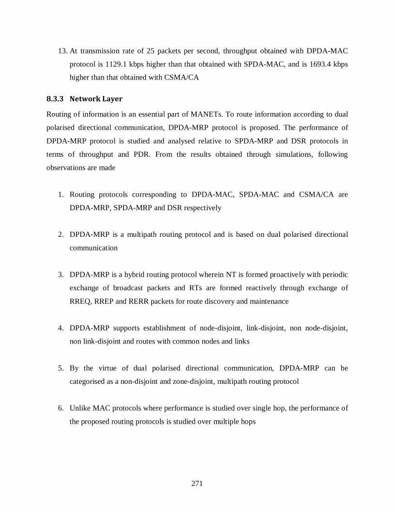
271

13. At transmission rate of 25 packets per second, throughput obtained with DPDA-MAC

protocol is 1129.1 kbps higher than that obtained with SPDA-MAC, and is 1693.4 kbps

higher than that obtained with CSMA/CA

8.3.3 Network Layer

Routing of information is an essential part of MANETs. To route information according to dual

polarised directional communication, DPDA-MRP protocol is proposed. The performance of

DPDA-MRP protocol is studied and analysed relative to SPDA-MRP and DSR protocols in

terms of throughput and PDR. From the results obtained through simulations, following

observations are made

1. Routing protocols corresponding to DPDA-MAC, SPDA-MAC and CSMA/CA are

DPDA-MRP, SPDA-MRP and DSR respectively

2. DPDA-MRP is a multipath routing protocol and is based on dual polarised directional

communication

3. DPDA-MRP is a hybrid routing protocol wherein NT is formed proactively with periodic

exchange of broadcast packets and RTs are formed reactively through exchange of

RREQ, RREP and RERR packets for route discovery and maintenance

4. DPDA-MRP supports establishment of node-disjoint, link-disjoint, non node-disjoint,

non link-disjoint and routes with common nodes and links

5. By the virtue of dual polarised directional communication, DPDA-MRP can be

categorised as a non-disjoint and zone-disjoint, multipath routing protocol

6. Unlike MAC protocols where performance is studied over single hop, the performance of

the proposed routing protocols is studied over multiple hops

272

7. Throughput and PDR provided by DPDA-MRP are the highest among three routing

protocols considered for this study

8. For channel capacity of 54 Mbps, node density of 100 nodes per unit area, packet

transmission rate of 1 packet per second and node mobility of 3 m/s, PDR of; DPDA-

MRP is 95%; SPDA-MRP is 35%; and DSR is 11%. When rate of packet transmission is

increased to 25 packets per second, keeping all other simulation parameters the same,

PDR obtained for DPDA-MRP is 44%, for SPDA-MRP it is 19% and that for DSR is 6%

9. Maximum throughput is obtained with packet transmission rate of 5 packets per second.

This trend is observed for all the three routing protocols and for all values for channel

capacity. The initial increase in throughput with increase in the rate of packet

transmission is due to the increase in the number of packets transmitted per unit time.

However further increase in rate of packet transmission leads to increased traffic load on

the network, resulting in increased network congestion

10. With 5 packets transmitted per unit time, channel capacity of 54 Mbps, node density of

100 nodes per unit area and mobility of nodes as 3 m/s, throughput for DPDA-MRP is

351.1 kbps, for SPDA-MRP it is 57 kbps and for DSR it is 8.6 kbps

8.4 Suggestions for Future Work

Research involves continuous improvement of existing work. Research proposed in this thesis

improves the existing methods and techniques at physical, MAC and network layers of the

protocol stack for enhanced operation of MANETs. However, this research is only an

incremental contribution towards the developmental efforts carried by the research community to

enhance the operation and performance of MANETs.

This section presents some suggestions which can be accommodated to advance this research

further. The suggestions are categorised for physical, MAC and network layers.

273

8.4.1 Suggestions for Improvement in Physical Layer

This thesis presented the use of dual polarised directional communication to combat interference

and increase throughput of the network. The present work can be further enhanced to include

simultaneous communication over multiple channels in orthogonal polarisations. This would

allow another dimension for data communication to reduce interference and increase throughput

of MANETs which face limitation of bandwidth. However, this introduces additional design and

implementation challenges, some of which are mentioned below

1. Antenna design for dynamically switching between channels and polarisations to carry

out successful communication between nodes

2. Nodes carrying out multichannel communication can face the problem of deafness,

wherein one node can send communication request to another node which is tuned to a

different channel and thus deaf towards the requests of first node. A solution to avoid

deafness with multichannel communication needs to be suggested

3. Methods to overcome the problems of hidden and exposed nodes in dual polarisation

based multichannel communication need to be investigated

4. Communication in MANETs takes place over multiple hops. Multihop communication

involves routing of information. To exploit the benefits multichannel communication

over dual polarisation, an appropriate routing protocol should be designed

5. Presently, the implemented solution only provides a provision for power control. The

performance of implemented solution with power control has not been studied through

simulations. In future, the implemented protocol can be extended to incorporate dynamic

power control for energy efficient communication

6. In future, the study of performance of the proposed dual polarised directional antenna

based communication can be extended to VANETs. This will require inclusion of

274

mobility models based on traffic, traffic regulations and road topologies, and DSRC

based IEEE 802.11p communication standard, in the present implementation

7. To gain wider understanding of the effect of change in communication range on the

performance of the proposed protocol, in future, simulations can be carried out for

different values of communication range, and performance of the proposed protocol can

be analysed

With present solution of dual polarised directional communication, in case of deafness, only two

nodes get benefitted with the availability two orthogonal polarisations. In case a third node

wishes to establish communication with a node which is busy communicating with two other

nodes over two different orthogonal polarisations, the third node needs to wait for the

appropriate NAV duration. Incorporation of multichannel communication along with dual

polarisation can provide additional options to avoid more nodes from getting affected with the

problem of deafness.

8.4.2 Suggestions for Improvement in MAC layer

This thesis presented DPDA-MAC protocol for controlling the access to the medium, to support

dual polarised directional communication in MANETs. This protocol involves the exchange of

intermediate Link ID broadcasts, which leads to increase in per-hop delay. Also, as observed

from simulation results, per-hop delay of DPDA-MAC is higher than that of SPDA-MAC. This

can be attributed to the explicit requirement of a node to wait for the availability of vertical

polarisation for transmission of intermediate broadcasts, even if horizontal polarisation is free for

data transmission. The per-hop delay with DPDA-MAC protocol is tolerable when viewed with

the realised advantage of increased throughput. However, a solution which can avoid the delay in

transmission of data packets caused due to transmission of broadcasts only in vertical

polarisation is still desirable for the improved performance of DPDA-MAC protocol.

8.4.3 Suggestions for Improvement in Network Layer

To exploit the benefits of dual polarised directional communication, this thesis proposed DPDA-

MRP. DPDA-MRP is a multipath routing protocol which discovers multiple routes between

source and destination nodes, but uses the one with least number of hops at a time. This protocol

275

can be further enhanced to support load sharing by simultaneous use of multiple paths between

source and destination. For this, it is required to incorporate the following

1. Appropriate load sharing algorithm needs to be designed and implemented

2. Designed load sharing algorithm should consider effects of unavailability of same

polarisation between nodes within communication range in a path, and methods to

overcome the same

3. Effect on load sharing in case of path breakages due to node mobility should be

considered

4. Delays in packet arrival or loss of packets while assembling the packets received from

multiple paths needs to be handled

276

REFERENCES

Abdullah, A. A., Cai, L.,and Gebali, F. (2012) ‘DSDMAC: Dual sensing directional MAC

protocol for ad hoc networks with directional antennas’. IEEE Transactions on Vehicular

Technology, IEEE, Volume 61, Issue 3, 1266-1275.

Abolhasan, M., Wysocki, T., and Dutkiewicz, E. (2004). ‘A review of routing protocols for

mobile ad hoc networks’. Ad hoc networks, Volume 2, Issue 1. Elsewier, 1-22.

Ahmed, N., Ahmed, Z. I., Saikia, S. I., and Hussain, I., (2015), ‘Augmentation of Directional and

Sector Antenna Support in NS2’. In proceedings of IEEE International Conference

onComputational Intelligence and Networks (CINE), 12th - 13th January, Bhubaneshwar,

Odisha, India. IEEE, 68-73.

Alagar, S.,Venkatesan, S., and Cleaveland, J.R. (1995)‘Reliable boradcast in mobile wireless

networks’. In Proceedings of IEEEMilitary Communication Conference (MILCOM’95),

San Diego, CA. IEEE 236-240.

Anastasi, G., Conti, M., and Gregori, E. (2004) ‘IEEE 802.11 ad hoc networks: protocols,

performance and open issues’. In Mobile Ad Hoc Networking. Chapter 3, IEEE Press, 69-

116.

Arora, A., Krunz, M.,and Muqattash, A. (2004) ‘Directional medium access protocol (DMAP)

with power control for wireless ad hoc networks’. In Proceedings of IEEE Global

Telecommunication Coference (GLOBECOM’04), Dallas, Texas, USA, 29 November-3

December. IEEE, Volume 5, 2797-2801.

Bai, F., and Helmy, A., (2004), ‘A survey of mobility models in wireless adhoc networks’. Book

Chapter in Wireless Adhoc and Sensor Networks. Kluwer Academic Publishers, 1-30.

277

Bazan, O.,and Jaseemuddin, M.(2011) ‘On the Design of Opportunistic MAC Protocols for

Multihop Wireless; Networks with Beamforming Antennas’. IEEE Transactions on Mobile

Computing, IEEE, Volume 10, Issue 3, 305-319.

Belding-Royer, E. M. (2004) ‘Routing approaches in mobile ad hoc networks’. In Mobile Ad

Hoc Networks, Chapter 10, IEEE press, 275-300.

Bellofiore, S., Foutz, J., Govindrajalu, R., Bahceci, I., Balanis, C. A., Spanias, A.S., Capone,

J.M., and Doman, T.M. (2002) ‘Smart Antenna System Analysis, Integration and

Performance for Mobile Ad-Hoc Networks (MANETs)’. IEEE Transactions on Antennas

and Wave Propagation, Volume 50, Issue 5,IEEE, 571-581.

Bettstetter, C., and Wagner, C. (2002) ‘The Spatial Node Distribution of the Random Waypoint

Mobility Model’. In WMAN,Volume 11, 41-58.

Bhargavan, V.,Demers, A.,Shenker, S., and Zhang, L. (1994)‘MACAW: A media access

protocol for wireless LANs’. In Proceedings of the conference on Communications

architectures, protocols and applications (SIGCOMM’94), London, UK, 31 August- 2

September. ACM, 212-225.

Black, D. C., Donovan, J., Bunton, B., and Keist, A. (2009), ‘SystemC: From the Ground Up’,

Second Edition : From the Ground Up, Volume 71, Springer Science & Business Media.

Blake, R., (2000) ‘Wireless Communication Technology’. 1st Edition, Delmar Thomson

Learning.

Boukerche, A. and Bononi, L. (2004) ‘Simulation and mobile modelling of wireless, mobile and

ad-hoc networks’. In Mobile Ad Hoc Networks, Chapter 14, IEEE press, 373-409.

Burton, M. (2009) ‘802.11 Arbitration’. In Certified Wireless Network Professional, white paper,

1-24.

278

Capone, A., Martignon, F.,and Fratta, L. (2008)‘Directional MAC and routing schemes for

power controlled wireless mesh networks with adaptive antennas’.Ad Hoc Networks,

Elsevier, Volume 6, Issue 6, Volume 6, Issue 6, 936-952.

Chan, A.,and Liew, S. C. (2006) ‘Merit of PHY-MAC cross-layer carrier sensing: a MAC

address based Physical Carrier Sensing scheme for solving hidden-node and exposed-node

problems in large-scale Wi-Fi networks’. In Proceedings of 31st Annual IEEE Conference

on Local Computer Networks (LCN’06), Tampa, Florida, USA, 14-16 November. IEEE,

871-878.

Chiang, C. C., Wu, H. K., Liu, W.,and Gerla, M. (1997) ‘Routing in clustered multihop, mobile

wireless networks with fading channel’. In Proceedings of IEEE SICON, Volume 97, 197-

211.

Chiasserini, C. F., and Rao, R. R. (2003) ‘Coexistence mechanisms for interference mitigation in

the 2.4-GHz ISM band’. In IEEE Transactions on Wireless Communications, Volume 2,

Issue 5, IEEE, 964-975.

Chilukuri, S. (2012) ‘Design and development of an energy efficient multipath routing protocol

using directional antenna for MANETs’. M.Sc (Engg.) Dissertation in Computer Science

and Networking, Coventry University, UK.

Choudhury, R. R., and Vaidya, N. H. (2004) ‘Deafness: A MAC problem in ad hoc networks

when using directional antennas’. In Proceedings of the 12th IEEE International

Conference onNetwork Protocols (ICNP’04), Berlin, Germany, 5-8 October. IEEE, 283-

292.

Choudhury, R. R., Yang, X., Ramanathan, R., and Vaidya, N. H. (2006) ‘On designing MAC

protocols for wireless networks using directional antennas’. In IEEE Transactions on

Mobile Computing, Volume 5, Issue 5, IEEE, 477-491.

279

Choudhury, R. R., Yang, X., Ramanathan, R.,and Vaidya, N. H. (2002)‘Using directional

antennas for medium access control in ad hoc networks’.In Proceedings of the 8th annual

international conference on Mobile computing and networking (Mobicom’02), Atlanta,

Georgia, USA, 23-28 September. ACM, 59-70.

Dai, H. N., Ng, K. W.,and Wu, M. Y. (2007) ‘A busy-tone based MAC scheme for wireless ad

hoc networks using directional antennas’. In Proceedings of IEEE Global

Telecommunications Conference (GLOBECOM’07), Washington, DC, USA, 26-30

November. IEEE, 4969-4973.

Deng, D. J., Ke, C. H., Chao, H. C., and Huang, Y. M. (2010) ‘On delay constrained CAC

scheme and scheduling policy for CBR traffic in IEEE 802.11 e wireless LANs’. In

Wireless Communications and Mobile Computing, Volume 10, Issue 11, Wiley Online

Library, 1509-1520.

Dhande, P. (2009) ‘Antennas and its Applications’. In DRDO Science Spectrum, 66-78.

Ding, Y., Wang, X., Shen, H.,and Guo, P. (2010) ‘Media Access Control Protocol Based on

Hybrid Antennas in Ad Hoc Networks’. In Proceedings of 7thInternational Conference on

Ubiquitous Intelligence & Computing and Autonomic & Trusted

Computing(UIC/ATC’10), Xi’an, Shaanxi, China, 26-29 October. IEEE, 148-153.

Durvy, M., Dousse, O., and Thiran, P. (2007) ‘Modeling the 802.11 protocol under different

capture and sensing capabilities’. In 26th IEEE International Conference on Computer

Communications, INFOCOM’07. 6-12 May, Anchorage, Alaska, USA. IEEE, 2356-2360.

Egbogah, E., Shi, L., and Fapojuwo, A. (2011) ‘Optimal Hidden Node Area for Enhancing

Routing Protocol Performance in IEEE 802.11 Multihop MANETs’.Journal of Electrical

and Computer Engineering, Hindawi Publishing Corporation, Volume 2011, Article ID

402308, 1-7.

280

El-Osery, A. I., Baird, D., Memon, M., Bruder, S.,and Wedeward, K. (2004) ‘Power control in

ad hoc networks: an overview’. Proceedings of SPIE, Volume 5440, 126-133.

Fakih, K., Diouris, J. F.,and Andrieux, G. (2006) ‘BMAC: beamformed MAC protocol with

channel tracker in MANET using smart antennas’. In Proceedings of the 9th European

Conference on Wireless Technology, Manchester, UK, 10-12 September. IEEE, 185-188.

Feeney, L. M. (2004) ‘Energy-efficient communication in ad hoc wireless networks’. In Mobile

Ad Hoc Networking. Chapter 11, IEEE Press, 301-327.

Fiore, M., Harri, J., Filali, F. and Bonnet, C. (2007) ‘Vehicular mobility simulation for

VANETs’. In Proceedings of the 40th Annual Simulation Symposium, ANSS'07, 26-28

March, Washington, DC, USA. IEEE Computer Society, 301-309.

Forouzan, B. A. (2007) ‘Wireless LANs’. In Data Communication and Networking. Chapter 14,

Networking Series, Tata Mcgraw-Hill, 421-444.

Garcia-Luna-Aceves, J. J.,and Fullmer, C. L. (1999) ‘Floor acquisition multiple access (FAMA)

for packet-radio networks’. Mobile Networks and Applications, Kluwer Academic

Publishers, Volume 4, Issue 3, 157-174.

Gossain, H., Cordeiro, C., Cavalcanti, D.,and Agrawal, D. P.,(2004) ‘The deafness problems and

solutions in wireless ad hoc networks using directional antennas’. IEEE Global

Telecommunications Conference Workshops, Globecom Workshops, Dallas, Texas, USA,

29 November-3 December. IEEE, 108-113.

Gossain, H., Joshi, T., Cordeiro, C., and Agrawal, D. P. (2005). ‘A cross-layer approach for

designing directional routing protocol in MANETs’. In Wireless Communications and

Networking Conference (WCNC’ 2005), 13-17 March, New Orleans, LA, USA, Volume 4,

IEEE, 1976-1981.

281

Haas, Z. J., Pearlman, M. R.,and Samar, P.,(2002) ‘Zone routing protocol for ad-hoc networks’.

draft-ietf-manet-zone-zrp-04. txt.

Haas, Z.J., and Deng, J. (2002) ‘Dual Busy Tone Multiple Access (DBTMA): A Multiple Access

Scheme for Ad Hoc Networks’. IEEE Transactions on Communications, IEEE

Communications Society, Volume 50, Issue 6, 975-985.

Hadjadj-Aoul, Y.,and Naït-Abdesselam, F. (2008) ‘On Physical-Aware Directional MAC

Protocol for Indoor Wireless Networks’. In Proceedings of IEEE Global

Telecommunications Conference (GLOBECOM’08), New Orleans, LA, USA, 30

November - 4 December. IEEE, 1-5.

Halford, T. R., and Chugg, K. M. (2011) ‘The reliability multihop routes with autonomous

cooperation’. In UCSD Information Theory and Applications Workshop (invited), La Jolla,

CA.

Hayajneh, T., Krishnamurthy, P., Tipper, D. and Kim, T. (2009) ‘Detecting malicious packet

dropping in the presence of collisions and channel errors in wireless ad hoc networks’. In

proceedings of IEEE International Conference onCommunications, 2009. ICC'09. IEEE, 1-

6.

Hiertz, G. R., Denteneer, D., Stibor, L., Zang, Y., Costa, X. P., and Walke, B. (2010) ‘The IEEE

802.11 universe’. IEEE Communications Magazine,Volume 48, Issue 1, IEEE, 62-70.

Hong-Ning, D. A. I., Kam-Wing, N. G., Min-You, W. U., and Bo, L. I. (2008) ‘Collision-

Tolerant Transmission with Narrow-beam Antennas’. International Journal of

Communications, Network and System Sciences, Volume 1, Issue 4, Scientific Research

Publishing, 285-385.

Hou, Y. T., Shi, Y., Sherali, H. D.,and Wieselthier, J. E. (2005) ‘Online lifetime-centric multicast

routing for ad hoc networks with directional antennas’. In Proceedings of 24thAnnual Joint

282

Conference of the IEEE Computer and Communications Societies (INFOCOM’05), Miami,

Florida, 13-17 March. IEEE, Volume 1, 761-772.

Hu, L., and Evans, D. (2004) ‘Using Directional Antennas to Prevent Wormhole Attacks’. In

Network and Distributed System Security Symposium (NDSS 2004), San Diego,

California, USA, February 2004, 1-11.

Huang, Z., Shen, C.C., Srisathapornphat, C.,and Jaikaeo, C. (2002)‘A busy-tone based

directional MAC protocol for ad hoc networks’. Proceedings of IEEE Military

Communication Conference (MILCOM’02), Anaheim, CA, 7-10 October. IEEE, Volume

2, 1233-1238.

IEEE 802 LAN/MAN Standards Committee (1999). ‘Wireless LAN medium access control

(MAC) and physical layer (PHY) specifications’. IEEE standard 802.11. IEEE Computer

Society.

Jacquet, P., Muhlethaler, P., Clausen, T., Laouiti, A., Qayyum, A.,and Viennot, L.,(2001)

‘Optimized link state routing protocol for ad hoc networks’. Proceedings of IEEE

International Multi Topic Conference (INMIC’01), Technology for 21st Century, Lahore,

Pakistan, 28-30 December. IEEE, 62-68.

Jain, K., Padhye, J., Padmanabhan, V. N.,and Qiu, L. (2005) ‘Impact of interference on multi-

hop wireless network performance’. Wireless Networks, Springer, Volume 11, Issue 4,

471-487.

Jakllari, G., Broustis, I., Korakis, T., Krishnamurthy, S. V.,and Tassiulas L. (2005) ‘Handling

asymmetry in gain in directional antenna equipped ad hoc networks’. IEEE 16th

International Symposium on Personal, Indoor and Mobile Radio Communications

(PIMRC’05), Berlin, Germany, 11-14 September. IEEE, Volume 2, 1284-1288.

283

Jasani, H., and Yen, K., (2006) ‘Performance Improvement using Directional Antennas in Ad

Hoc Networks’. International Journal of Computer Science and Network Security, Volume

6, Issue 6, 180-188.

Javan, N. T.and Dehghan, M. (2007) ‘Reducing end-to-end delay in multi-path routing

algorithms for mobile ad hoc networks. Mobile Ad-Hoc and Sensor Networks’, Springer

Berlin Heidelberg, Volume 4864, 715-724.

Jayasuriya, A., Perreau, S., Dadej, A., and Gordon, S. (2004)‘Hidden vs exposed terminal

problem in ad hoc networks’. Proceedings of Australian Telecommunication Networks and

Applications Conference (ATNAC’04), Sydney, Australia.

Jennifer, J., Liu, N., and Chlamtac, I. (2004) ‘Mobile ad hoc networking with a view of 4g

wireless: imperatives and challenges’. In Mobile Ad Hoc Networking. Chapter 1, IEEE

Press, 1-45.

Jiang, L.B., and Liew, S. C. (2008) ‘Improving throughput and fairness by reducing exposed and

hidden nodes in 802.11 networks’. In IEEE Transactions on Mobile Computing, Volume 7,

No. 1, 34-49.

Joa-Ng, M.,and Lu, I. T. (1999) ‘A peer-to-peer zone-based two-level link state routing for

mobile ad hoc networks’. IEEE Journal on Selected Areas in Communications, Volume 17,

Issue 8, 1415-1425.

Johnson, D. B., Maltz, D. A.,and Broch, J. (2001) ‘DSR: The dynamic source routing protocol

for multi-hop wireless ad hoc networks’. In Ad Hoc Networking, edited by Charles E.

Perkins, Addison-Wesley, Chapter 5, 139-172.

Jung, S., Lee, S.and Han, K. (2009) ‘A DMAC Protocol to improve spatial reuse by managing

the NAV table of the nodes in VANET’. 2nd International Conference on Computer and

Electrical Engineering (ICCEE’09), Dubai, 28-30 December. IEEE, 387-390.

284

Kadambi, G. R., and Sullivan, J. L. (2003) U.S. Patent No. 6,639,560. Washington, DC: U.S.

Patent and Trademark Office.

Keowsawat, P., Phongcharoenpanich, C., Kosulvit, S., Takada, J. I.,and Krairiksh, M. (2009)

‘Mutual information of MIMO system in a corridor environment based on double

directional channel measurement’. Journal of Electromagnetic Waves and Applications,

Volume 23, Issue 8-9, 1221-1223.

Khalid, M., Le, X. H., Ra, I. H., and Sankar, R. (2011) ‘Polarization-based cooperative

directional mac protocol for ad hoc networks’. Ad Hoc Networks, Elsevier, Volume 11,

Issue 4, 1522-1538.

Ko, Y. B., and Vaidya, N. H. (2000) ‘Location Aided Routing (LAR) in mobile ad hoc

networks’. In Wireless Networks, Springer, Volume 6, Issue 4, 307-321.

Ko, Y. B., Shankarkumar, V.,and Vaidya, N. H. (2000) ‘Medium access control protocols using

directional antennas in ad hoc networks’. Proceedings of 19th Annual Joint Conference of

IEEE Computer and Communication Societies, (INFOCOM’00), Tel Aviv, 26-30 March.

IEEE, Volume 1, 13-21.

Korakis, T., Jakllari, G., and Tassiulas, L. (2003) ‘A MAC protocol for full exploitation of

directional antennas in ad-hoc wireless networks’. In Proceedings of the 4th ACM

international symposium on Mobile ad hoc networking & computing, MOBIHOC ’03,

ACM, 98-107.

Korakis, T., Jakllari, G.,and Tassiulas, L. (2008) ‘CDR-MAC: A protocol for full exploitation of

directional antennas in ad hoc wireless networks’. IEEE Transactions on Mobile

Computing, Volume 7, Issue 2, IEEE Computer Society, 145-155.

285

Kumar, V., Arunan, T., and Balakrishnan, N. (2003) ‘E-span: Enhanced-span with directional

antenna’. In Conference on Convergent Technologies for the Asia-Pacific Region,

TENCON ’03, October15-17, Bangalore, India.IEEE, Volume 2, 675-679.

Lee, E. J., Kang, C. N., Han, D., Yang, D. Y., and Jwa, J. (2006) ‘A Tone Dual-Channel DMAC

Protocol in Location Unaware Ad Hoc Networks’. Communications in Computing, 91-96.

Lee, S. J., and Gerla, M. (2000) ‘AODV-BR: Backup routing in ad hoc networks’. In Wireless

Communications and Networking Confernce, Chicago, USA, 23rd - 28th September.

Volume 3, IEEE, 1311-1316.

Lee, S. J.,and Gerla, M. (2001) ‘Split multipath routing with maximally disjoint paths in ad hoc

networks’. IEEE International Conference on Communication (ICC’01), Helsinki, 11-14

June. IEEE, Volume 10, 3201-3205.

Li, F. and Wang, Y. (2007) ‘Routing in vehicular ad hoc networks: A survey’. In Vehicular

Technology Magazine, Volume 2, Issue 2, IEEE, 12-22.

Li, J., Blake, C., De Couto, D. S., Lee, H. I.,and Morris, R. (2001)‘Capacity of ad hoc wireless

networks’. InProceedings of the 7th Annual International Conference on Mobile

Computing and Networking (Mobicom’01), New York, NY, USA, 61-69.

Li, M., Zhang, L., Li, V. O. K., Shan, X., and Ren, Y. (2005) ‘An energy-aware multipath

routing protocol for mobile ad hoc networks’. ACM Sigcomm Asia, Beijing, 10-12 April.

ACM, 166-174.

Lim, H.,and Kim, C. (2000) ‘Multicast tree construction and flooding in wireless ad hoc

networks’. 3rd ACM International Workshop on Modeling, Analysis and Simulation of

Wireless and Mobile Systems (MSWiM’00), Boston, 20 August. ACM, 61-68.

286

Lu, H., Li, J., Dong, Z.,and Ji, Y. (2011) ‘CRDMAC: An Effective Circular RTR Directional

MAC Protocol for Wireless Ad Hoc Networks’.7th International Conference on Mobile

Ad-hoc and Sensor Networks (MSN’11), Beijing, 16-18 December. IEEE, 231-237.

Lu, X., Fan, G.,and Hao, R. (2006) ‘A dynamic token passing MAC protocol for mobile ad hoc

networks’. International conference on Wireless Communications and Mobile Computing

(IWCMC’06), Vancouver, Canada, 3-6 July. ACM, 743-748.

Lu, X., Wicker, F. D., Towsley, D., and Xiong, Z. (2010) ‘Detection probability estimation of

directional antennas and omni-directional antennas’. Wireless personal communications,

Volume 55, Issue 1, Springer, 51-63.

Lu, X., Wicker, F., Lio, P., and Towsley, D. (2008) ‘Security estimation model with directional

antennas’. In Military Communications Conference, MILCOM ’08, 16-19 November, San

Diego, California. IEEE, 1-6.

Macker, J. P., and Corson, M. S. (2004) ‘Mobile ad hoc networks (MANETs): routing

technology for dynamic wireless networking’. In Mobile Ad Hoc Networking. Chapter 9,

IEEE Press, 255-273.

Macker, J.,and Team, S. (2008) ‘Simplified multicast forwarding for MANET’.Internet draft,

draft-ietf-manet-smf-08.txt,2008.

Marina, M. K.,and Das, S. R. (2001) ‘On-demand multipath distance vector routing in ad hoc

networks’. 9th International Conference on Network Protocols (ICNP’01), Riverside, CA,

USA, 11-14 November. IEEE, 14-23.

Meghanathan, N. (2010) ‘Performance comparison of link, node and zone disjoint multi-path

routing strategies and minimum hop single path routing for mobile ad hoc

networks’.International Journal of Wireless & Mobile Networks (IJWMN), Volume 2002,

Number 4, 13-29.

287

Mott, H. (1986) ‘Polarization in antennas and radar’. Wiley-Interscience, New York, Volume 1.

Mueller, S., Tsang, R.P.,and Ghosal, D. (2004) ‘Multipath routing in mobile ad hoc networks:

Issues and challenges’.In Performance Tools and Applications to Networked Systems.

Springer Berlin Heidelberg, 209-234.

Nasipuri, A., Li, K., and Sappidi, U. R. (2002) ‘Power consumption and throughput in mobile ad

hoc networks using directional antennas’.11thInternational Conference on Computer

Communications and Networks (ICCCN’02), Miami, 14-16 October. IEEE, 620-626.

Nasipuri, A., Ye, S., You, J., and Hiromoto, R. E. (2000) ‘A MAC protocol for mobile ad hoc

networks using directional antennas’. In proceedings of IEEE Wireless Communications

and Networking Confernce, WCNC 2000, Chicago, IL, USA, 23-28 September, IEEE,

Volume. 3, 1214-1219.

Nikaein, N., Labiod, H.,and Bonnet, C. (2000) ‘DDR: distributed dynamic routing algorithm for

mobile ad hoc networks’. 1st ACM international symposium on Mobile ad hoc networking

and computing (MobiHoc’00), Boston, 11 August. IEEE Press, 19-27.

Open SystemC Initiative, (2006), ‘IEEE standard SystemC language reference manual’. IEEE

Computer Society.

Padhye, J., Agarwal, S., Padmanabhan, V. N., Qiu, L., Rao, A.,and Zill, B. (2005) ‘Estimation of

link interference in static multi-hop wireless networks’. In Proceedings of the 5th ACM

SIGCOMM conference on Internet Measurement. USENIX Association. 305-310.

Pagani,E., and Rossi,G.P. (1997) ‘Reliable broadcast in mobile multihop packet networks’.

3rdAnnual ACM/IEEE International Conference on Mobile Computing and Networking

(MobiCom’97), Budapest, 26-30 September. ACM, 34-42.

288

Pagani, E., and Rossi, G.P. (1999) ‘Providing reliable and fault tolerant broadcast delivery in

mobile ad-hoc networks’. Mobile Networks and Applications, Springer, Volume 4, Issue 3,

175-192.

Park, V.,and Corson, M. S. (1997)‘Temporally-ordered routing algorithm (TORA) version 1

functional specification’. Internet-Draft, draft-ietf-manet-tora-spec-00. txt, 2-6.

Paul, U., Crepaldi, R., Lee, J., Lee, S. J., and Etkin, R. (2011) ‘Characterizing WiFi link

performance in open outdoor networks’. 8thAnnual IEEE Communications Society

Conference on Sensor, Mesh and Ad Hoc Communications and Networks (SECON’11),

Salt lake city, 27-30 June. IEEE, 251-259.

Peng, W., and Liu, X. (2000) ‘On the reduction of broadcast redundancy in mobile ad hoc

networks’.1st ACM international symposium on Mobile ad hoc networking and computing

(MobiHoc’00), Boston, 11 August. IEEE Press, 129-130.

Peng, W., and Liu, X. (2001) ‘AHBP: An efficient broadcast protocol for mobile ad hoc

networks’. Journal of Computer Science and Technology, Springer, Volume 16, Number 2,

114-125.

Perkins, C. E., and Bhagwat, P. (1994) ‘Highly dynamic destination-sequenced distance-vector

routing (DSDV) for mobile computers’.ACM SIGCOMM Computer Communication

Review. ACM, Volume 24, Number 4, 234-244.

Perkins, C., Belding-Royer, E. and Das, S. (2003) ‘RFC 3561-ad hoc on-demand distance vector

(AODV) routing’.Internet RFCs, 1-38.

Qayyum, A., Viennot, L., and Laouiti, A. (2000) ‘Multipoint relaying: An efficient technique for

flooding in mobile wireless networks’.Research report RR-3898, INRIA, 1-19.

Qualnet 4.5.1 Wireless Model Library (2008) ‘Abstract PHY Model’. Scalable Network

Technologies, Los Angeles, CA, 62.

289

Quan, X. L., Li, R. L., Wang, J. Y., and Cui, Y. H. (2012) ‘Development of a broadband

horizontally polarized omnidirectional planar antenna and its array for base stations’.

Progress In Electromagnetics Research, volume 128, 441-456.

Ramanathan, R. (2001) ‘On the performance of ad hoc networks with beamforming

antennas’.2nd ACM international symposium on Mobile ad hoc networking & computing

(MobiHoc’01), Long Beach, USA, 4-5 October. ACM, 95-105.

Ramanathan, R. (2004) ‘Antenna beamforming and power control for ad hoc networks’. In

Mobile Ad Hoc Networking. Chapter 5, IEEE Press, 139-173.

Ramanathan, R., Redi, J., Santivanez, C., Wiggins, D., and Polit, S. (2005) ‘Ad hoc networking

with directional antennas: a complete system solution’. In IEEE Journal on Selected Areas

in Communications, Volume 23, No. 3, 496-506.

Rappaport, T.S., (2004) ‘Wireless Communications: Principles and Practice’. 2nd Edition,

Pearson Education, India.

Saha, A. K., and Johnson, D. B. (2004) ‘Routing improvement using directional antennas in

mobile ad hoc networks’. In Global Telecommunications Conference, GLOBECOM'04,

29th November-3rd December, Dallas, Texas, USA. Volume 5, IEEE, 2902-2908.

Saha, D., Toy, S., Bandyopadhyay, S., Ueda, T.,and Tanaka, S. (2003) ‘An adaptive framework

for multipath routing via maximally zone-disjoint shortest paths in ad hoc wireless

networks with directional antenna’.Global Telecommunications Conference

(GLOBECOM'03), San Francisco, 1-5 December. IEEE, Volume 1, 226-230.

Sánchez, M., Giles, T.,and Zander, J. (2001)‘CSMA/CA with beam forming antennas in multi-

hop packet radio’.Swedish Workshop on Wireless Ad Hoc Networks. 63-69.

290

Sardouk, A., Senouci, S.M., Achir, N., and Boussetta, K. (2007) ‘Assessment of MANET

broadcast schemes in the application context of multiplayer video games’.6th ACM

SIGCOMM workshop on Network and system support for games(NetGames’07),

Melbourne, 19-20 September, ACM, 55-60.

Savvides, A., and Srivastava, M. B. (2004) ‘Location discovery’. In Mobile Ad Hoc Networking.

Chapter 8, IEEE Press, 231-254.

Seo, C. E., Leonardo, E. J., Cardieri, P., Yacoub, M. D., Gallego, D. M., and de Medeiros, A. A.

(2005). Performance of IEEE 802.11 in wireless mesh networks. In SBMO/IEEE MTT-S

International Conference on Microwave and Optoelectronics, Brasilia, DF, Brazil. IEEE,

363-367.

Sharma, R., Kadambi, G., Vershinin, Y. A.,and Mukundan, K. N. (2014)‘A survey of MAC layer

protocols to avoid deafness in wireless networks using directional antenna’. In Handbook

of Research on Progressive Trends in Wireless Communications and Networking. Chapter

19, edited by M. A. Matin. IGI Global. Volume 1, 479-517.

Shaw, J. A. (2013) ‘Radiometry and the Friis transmission equation’. In American Journal of

Physics, Volume 81, Issue 1, 33-37.

Shih, K. P., Liao, W. H., Chen, H. C.,and Chou, C. M. (2009) ‘On avoiding RTS collisions for

IEEE 802.11 based wireless ad hoc networks’.Computer Communications, Elsevier,

Volume 32, Issue 1, 69-77.

Shihab, E., Cai, L.,and Pan, J. (2009) ‘A distributed asynchronous directional-to-directional

MAC protocol for wireless ad hoc networks’.IEEE Transactions on Vehicular Technology,

IEEE, Volume 58, Issue 9, 5124-5134.

291

Shukla, D., Chandran-Wadia, L., and Iyer, S. (2003) ‘Mitigating the exposed node problem in

IEEE 802.11 ad hoc networks’. 12th International Conference onComputer

Communications and Networks (ICCCN’03), Dallas, 20-22 October, IEEE, 157-162.

Sikora, A., and Groza, V. F. (2005) ‘Coexistence of IEEE802. 15.4 with other Systems in the 2.4

GHz-ISM-Band’. In Instrumentation and Measurement Technology Conference, IMTC

’05, 16-19 May, Ottawa. Volume 3, IEEE, 1786-1791.

Srisathapornphat, C.,and Shen, C. C. (2003) ‘Energy consumption behavior and performance of

directional virtual carrier sensing schemes’. Wireless Communications and Networking

(WCNC’03), 20 March, New Orleans, IEEE, Volume 3, 1895-1900.

Subramanian, A. P., and Das, S. R. (2010)‘Addressing deafness and hidden terminal problem in

directional antenna based wireless multi-hop networks’.Wireless networks, Kluwer

Academic Publishers, Volume 16, Issue 6, 1557-1567.

Swaminathan, A., Noneaker, D. L.,and Russell, H. B. (2012) ‘The design of a channel-access

protocol for a wireless ad hoc network with sectored directional antennas’. Ad Hoc

Networks, Elsevier, Volume 10, Issue 3, 284-298.

Takai, M., Martin, J., and Bagrodia, R. (2001) ‘Effects of wireless physical layer modeling in

mobile ad hoc networks’. In Proceedings of the 2nd ACM international symposium on

Mobile ad hoc networking & computing, Mobihoc ’01, 4-5 October, Long Beach,

California, USA. ACM, 87-94.

Takai, M., Martin, J., Bagrodia, R.,and Ren, A. (2002) ‘Directional virtual carrier sensing for

directional antennas in mobile ad hoc networks’. 3rd ACM international symposium on

Mobile ad hoc networking & computing (MobiHoc’02). ACM, 183-193.

292

Takata, M., Bandai, M.,and Watanabe, T. (2005) ‘Performance analysis of a directional MAC

protocol for location information staleness in MANETs’.IPSJ Digital Courier, Volume 1,

518-527.

Talucci, F., Gerla, M., and Fratta, L. (1997) ‘MACA-BI (MACA By Invitation) A receiver

Oriented Access Protocol for Wireless Multihop Networks’. 8th IEEE International

Symposium on Personal, Indoor and Mobile Radio Communications (PIMRC’97),

Helsinki, 1-4 September, IEEE, Volume 2, 435-439.

Tang, K., and Gerla, M. (2000) ‘MAC layer broadcast support in 802.11 wireless networks’. In

21st Century Military Communications Conference Proceedings, MILCOM 2000, 22-25

October, Los Angeles, California, Volume 1, IEEE, 544-548.

Theodore, S. K. A., and Fidelis, S. D. (2013) ‘Throughput improved - adaptive CSMA MAC

protocol design with power optimistic for MANET’. In International Journal of

Engineering Science and Innovative Technology (IJESIT), Volume 2, Issue 3, 274-279.

Tobagi,F.A. and Klienrock, L. (1975) ‘Packet switching in radio channels: Part II - hidden

terminal problem in carrier sense multiple-access and busy-tone solution’. IEEE

Transactions on Communication, IEEE, Volume 23, Issue 12, 1417-1433.

Tseng, Y. C., Ni, S. Y., Che, Y. S.,and Sheu, J. P. (2002) ‘The broadcast storm problem in a

mobile ad hoc network’. Wireless Networks, Springer, Volume 8, Issue 2-3, 153-167.

Tseng, Y.C., Ni, S.Y., and Shih, E.Y. (2003) ‘Adaptive approaches to relieving broadcast storms

in a wireless multi-hop mobile adhoc network’. IEEE Transactions on Computers, IEEE,

Volume 52, Issue 5, 545-557.

USRobotics Technical Report, ‘Wireless Networking over Extended Range: Technology options

for optimizing long range wireless connectivity’. USRobotics Website (www.usr.com).

293

Valera, A., Seah, W. K. G.,and Rao, S. V. (2003)‘Cooperative packet caching and shortest

multipath routing in mobile ad hoc networks’. 22nd Annual Joint Conference of the IEEE

Computer and Communications, San Francisco, 30 March-3 April, IEEE, Volume 1, 260-

269.

Vassis, D., and Kormentzas, G. (2006) ‘Throughput analysis for IEEE 802.11 Ad Hoc networks

under the hidden terminal problem’. In IEEE Consumer Communications and Networking

Conference, CCNC’06, 8-10 January, Las Vegas, Nevada, USA. IEEE, 1273-1276.

Vella, J. M.,and Zammit, S. (2010)‘Performance improvement of long distance MIMO links

using cross polarized antennas’.15th IEEE Mediterranean Electrotechnical Conference

(MELECON’10), Valletta, 26-28 April, IEEE, 1287-1292.

Waharte, S.,and Boutaba, R. (2006) ‘Totally disjoint multipath routing in multihop wireless

networks’. International Conference of Communiations (ICC’06), Atlantic City, NJ, 17-20

October, IEEE, Volume 12, 5576-5581.

Wang, J., Fang, Y.,and Wu, D. (2005) ‘SYN-DMAC: A directional MAC protocol for ad hoc

networks with synchronization’. Military Communication Conference (MILCOM’05),

IEEE, Volume 4, 2258-2263.

Wang, L., Wu, K.,and Hamdi, M. (2012) ‘Combating hidden and exposed terminal problems in

wireless networks’. IEEE Transactions on Wireless Communication, Volume 11, Issue 11,

IEEE, 4204-4213.

Williams, B., and Camp, T. (2002) ‘Comparison of broadcasting techniques for mobile ad hoc

networks’. Proceedings of the 3rd ACM international symposium on Mobile ad hoc

networking and computing (Mobihoc'02), ACM, New York, 194-205.

294

Wu, C., and Li, V. (1987) ‘Receiver-initiated busy-tone multiple access in packet radio

networks’. Proceedings of the ACM workshop on Frontiers in computer communications

technology (SIGCOMM’87), ACM, New York, Volume 17, Issue 5, 336-342.

Xu, K., Gerla, M.,and Bae, S. (2003) ‘Effectiveness of RTS/CTS handshake in IEEE 802.11

based ad hoc networks’. Ad Hoc Networks, Elsevier, Volume 1, Number 1, 107-123.

Xu, S.,and Saadawi, T. (2001) ‘Does the IEEE 802.11 MAC protocol work well in multihop

wireless ad hoc networks?’. Communication Magazine, IEEE, Volume 39, Issue 6, 130-

137.

Yamamoto, K. and Yamamoto, M. (2007) ‘Performance Improvement of Ad Hoc Networks by

Deployment of Directional Antenna’.Information and Media Technologies, Volume 2,

Number 3, 907-913.

Yang, X., and Vaidya, N. H. (2002) ‘Priority scheduling in wireless ad hoc networks’. In

Proceedings of the 3rd ACM international symposium on Mobile ad hoc networking &

computing, Mobihoc ’02, Lausanne, Switzerland, June 9-11, ACM, 71-79.

Ye, Z., Krishnamurthy, S. V., and Tripathi, S. K. (2003) ‘A framework for reliable routing in

mobile ad hoc networks’.22ndAnnual Joint Conference of the IEEE Computer and

Communications (INFOCOM’03), 30 March-3 April, IEEE, Volume 1, 270-280.

Yeh, C. H., Zhou, H., Ho, P. H., and Mouftah, H. T. (2003) ‘A variable-radius multichannel

MAC protocol for high-throughput low-power heterogeneous ad hoc networking’.Global

Telecommunication Conference (GLOBECOM’03), 1-5 December, IEEE, Volume 3,

1284-1289.

Yildirim, F., and Liu, H. (2007) ‘Directional MAC for 60 GHz using Polarization Diversity

Extension (DMAC-PDX)’.Global Telecommunications Conference (GLOBECOM'07),

Washington, DC, 26-30 November, IEEE, 4697 - 4701.

295

Yousefi, S., Mousavi, M. S. and Fathy, M. (2006) ‘Vehicular ad hoc networks (VANETs):

challenges and perspectives’. In Proceedings of the 6th International Conference on ITS

Telecommunications, 21-23 June, Chengdu, China. IEEE, 761-766.

Zaggoulos, G., Nix, A.,and Halls, D. (2010)‘Novel antenna configurations for wireless

broadband vehicular communications’. 6th International Conference onWireless and

Mobile Communications (ICWMC), Valencia, 20-25 September, IEEE, 21-26.

Zhou, Y., and Nettles, S. M. (2005) ‘Balancing the hidden and exposed node problems with

power control in CSMA/CA-based wireless networks’. IEEE Wireless Communications

and Networking Conference, New Orleans, LA, USA, 13-17 March, IEEE, Volume 2, 683-

688.

296

APPENDIX 1

A1.1 Introduction

This appendix presents implementation details of the SystemC based simulator developed to

overcome specific shortcomings of commercial/open source network simulators relevant to this

research. The simulators considered for implementation and their limitations are discussed,

which lead to the need for developing the simulator used for work carried out in this thesis.

Components of the developed simulator are explained, along with their functionality.

Implementation details for enabling dual polarised directional communication between the nodes

and processing of messages exchanged between the nodes are presented. Portions of code are

also included to present an insight to the implementation. Scenarios to validate the functionality

of the developed simulator are also presented.

A1.2 Simulators Considered for Implementation and Their Limitations

To simulate dual polarised directional communication, Qualnet simulation tool was considered

because it has been popularly used in existing literature for simulating directional

communication in MANETs (Choudhury et al. 2002), (Xu, Gerla and Bae 2003), (Choudhury

and Vaidya 2004) and (Hadjadj-Aoul and Naït-Abdesselam 2008). On further study of features

of Qualnet simulator it was also observed that Qualnet supports feature of antenna polarisation as

well (Qualnet 4.5.1 Wireless Model Library 2008). Hence, Qualnet was thought to be as the

appropriate choice for carrying out simulations for dual polarised directional antenna. Therefore,

initial simulations to prove interference mitigation when interfering links are configured to

communicate over orthogonal polarisations (presented in Chapter 3) were carried out

successfully using research license of Qualnet version 4.5. However, during these simulations it

was also noticed that in Qualnet, the antenna on a node can be configured to use only one

polarisation at a time, implying that a directional antenna can be configured to work in either

vertical or horizontal polarisation at a time and it cannot be configured to support two orthogonal

polarisations (both vertical and horizontal polarisations) simultaneously, which is an inherent

requirement for operation of the dual polarised directional communication presented in this

thesis. Further into the implementation and through consultations with Qualnet Tech Support it

was learnt that Scalable Network Technologies (SNT), developers of the Qualnet Simulation

297

Tool, have not given access to parts of physical layer models to the users in order to protect their

intellectual property rights. Operation of the proposed dual polarised directional antenna based

DPDA-MAC and DPDA-MRP requires modification to the existing physical layer in Qualnet, to

enable simultaneous use of orthogonal polarisations and dynamic switching of antenna over

different modes of operation. Due to limited access to physical layer models, implementation of

the proposed dual polarised directional antenna based DPDA-MAC and DPDA-MRP protocols

could not be carried out in Qualnet.

To avoid getting into difficulties of limited access to proprietary implementation of commercial

tools, it was planned to explore availability of open source tools for simulation study of the

proposed dual polarised directional antenna based DPDA-MAC and DPDA-MRP protocols. The

Network Simulator - 2 (NS2) is an open source tool which is popular among researchers to carry

out simulations of MANETs (Peng and Liu 2000) and (Valera, Seah and Rao 2003). The

implementation of NS2.34 was studied and explored to check its feasibility to support dual

polarised directional communication. However, it did not have a built in directional antenna

model (Ahmed et al. 2015) and no concept of antenna polarisation was present in the available

antenna models.

Therefore, it was decided to implement a simulator in C++/SystemC that could support

simultaneous communication in orthogonal polarisations (vertical and horizontal). SystemC was

chosen for the following reasons (Black et al, 2009) and (Open SystemC Initiative 2006)

1. SystemC is a set of C++ classes and macros

2. It has notion of time, i.e, it can simulate time

3. Supports multithreaded programming (simulation of concurrent processes)

4. Provides an event-driven simulation kernel in C++

5. Open source, mature and tested

For the developed simulator, SystemC 2.3.0 was used. Details about the developed simulator are

given in Section A.3.

298

A1.3 Details of the Developed Simulation Tool

The schematic for top level implementation of the developed simulation tool is shown in Figure

A1. Here, the environment, medium and mobile node are class objects derived from SystemC’s

sc_module class. These objects are created at the start of the simulation, and stay throughout the

simulation. The packets exchanged in the network are developed as C++ class objects. These are

dynamic objects which are created by the transmitters and passed through the medium to the

receivers, where they are retained till needed.

Environment: The mobile nodes and medium instances are created and connected in the

environment. The number of nodes, their speed and position are decided by the scenario method

which is a member of the environment. The environment class creates multiple instances of

mobile node class to generate multiple mobile nodes based on requirement by the scenario. The

scenario method also calls the hook methods of mobile nodes to initiate packet transmission.

Figure A1 Top Level Implementation of the Developed Simulator

Medium: This class implements functionality of the medium. It has an array of ports that mobile

nodes can attach to transmit and receive packets. This block maintains the information about

location and velocity (speed and direction) of nodes. The X, Y coordinates (position) of nodes

having non-zero speed is updated periodically. Packets transmitted by nodes are first received by

the medium and methods in the medium forward the packets to prospective receiver nodes based

on their distance and direction from the transmitting nodes. The medium checks the factors such

as transmitting node, polarisation of transmission, type of transmission (directional or

omnidirectional), beam number for directional transmission, prospective receivers (based on

distance and direction from receiving node). If a medium finds that receiver thread of a node is

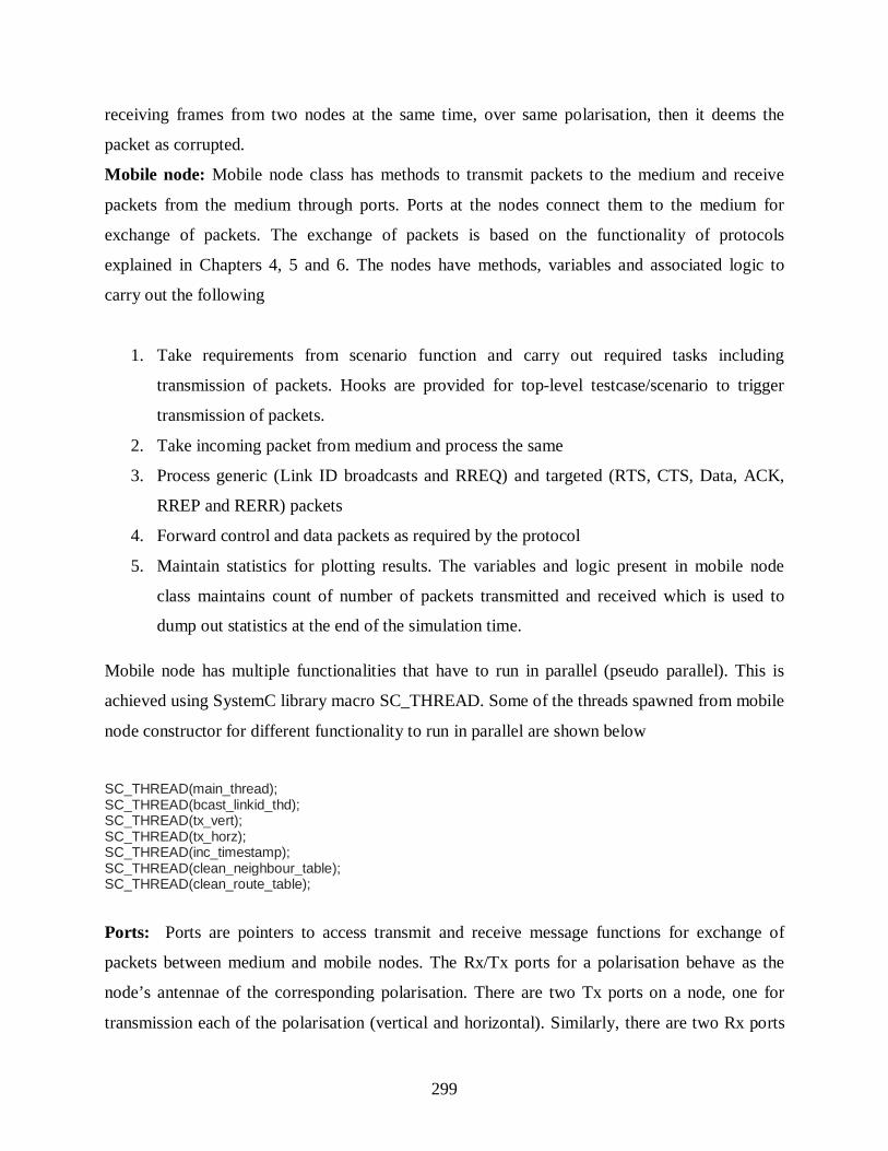
299

receiving frames from two nodes at the same time, over same polarisation, then it deems the

packet as corrupted.

Mobile node: Mobile node class has methods to transmit packets to the medium and receive

packets from the medium through ports. Ports at the nodes connect them to the medium for

exchange of packets. The exchange of packets is based on the functionality of protocols

explained in Chapters 4, 5 and 6. The nodes have methods, variables and associated logic to

carry out the following

1. Take requirements from scenario function and carry out required tasks including

transmission of packets. Hooks are provided for top-level testcase/scenario to trigger

transmission of packets.

2. Take incoming packet from medium and process the same

3. Process generic (Link ID broadcasts and RREQ) and targeted (RTS, CTS, Data, ACK,

RREP and RERR) packets

4. Forward control and data packets as required by the protocol

5. Maintain statistics for plotting results. The variables and logic present in mobile node

class maintains count of number of packets transmitted and received which is used to

dump out statistics at the end of the simulation time.

Mobile node has multiple functionalities that have to run in parallel (pseudo parallel). This is

achieved using SystemC library macro SC_THREAD. Some of the threads spawned from mobile

node constructor for different functionality to run in parallel are shown below

SC_THREAD(main_thread); SC_THREAD(bcast_linkid_thd); SC_THREAD(tx_vert); SC_THREAD(tx_horz); SC_THREAD(inc_timestamp); SC_THREAD(clean_neighbour_table); SC_THREAD(clean_route_table);

Ports: Ports are pointers to access transmit and receive message functions for exchange of

packets between medium and mobile nodes. The Rx/Tx ports for a polarisation behave as the

node’s antennae of the corresponding polarisation. There are two Tx ports on a node, one for

transmission each of the polarisation (vertical and horizontal). Similarly, there are two Rx ports

300

on a node, one for transmission each of the polarisation (vertical and horizontal).The fifth port is

the GPS port through which the mobile node fetches its coordinates from the medium. Authors in

(Ko and Vaidya 2000), (Huang et al. 2002) and (Savvides and Srivastava 2004) have considered

GPS for determination of location of the mobile nodes in MANETs.In medium class, the

tx_msg_function () is used for data transmission from node to medium. The mobile node’s Tx

port is a pointer to medium to access the tx_msg_function (). In mobile node class, there are two

functions to receive message called as rx_msg_start () and rx_msg_end () functions. The Rx port

is a pointer to mobile node to access these functions for reception of data from medium to mobile

node. The GPS port fetches location coordinates of mobile nodes from the medium (through a

global variable node_pos_vel () maintained at the medium). The nodes include this location

information in the Link ID broadcasts to inform their neighbour nodes about their location.

Using this information a NT (Table 4-1) is maintained as explained in Section 4.3. The

neighbour table cleanup thread updates the neighbour table periodically (every 1000 ms). Portion

of code for the same is shown below. Similar logic is used for cleanup of routing table.

void mobile_node :: clean_neighbour_table() {

std::map<node_id_typ , bcast_frame_neighb_table_struct * >::iterator curr , end; base_frame *frame; timestamp_typfrm_time , diff; while(1) {

// wait is a systemc function to implement delay wait(NEIGHBOUR_TABLE_CLEAN_CYCLE_DUR , SC_MS); Logic to check timestamps and remove old entries

} }

Scenario: The specifications of the scenario to be simulated are presented in scenario file. In

scenario parameters such as number of nodes, channel capacity, node mobility, terrain size and

communication distance are provided. An example scenario file is shown below.

// Define number of nodes #define NUM_NODES 20 #define NUM_TXRS 5 #define SEED NUM_NODES #define NUM_PKTS_PER_SECOND 1 #ifndef SCENARIO_H // { #define SCENARIO_H #include "env.h" extern std::vector node_pos_vel; void env::scenario() {

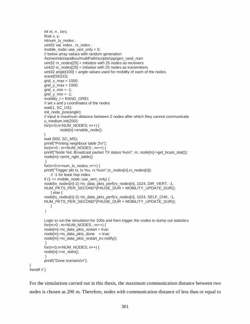
301

int m, n , txrs; float x, y; intnum_tx_nodes ; uint32 val, index , tx_index ; mobile_node::use_vert_only = 0; // below array values with random generation /home/rinki/sandbox/multiPath/scripts/cpp/gen_rand_num uint32 rx_nodes[25] = initialize with 25 nodes as receivers uint32 tx_nodes[25] = initialize with 25 nodes as transmitters uint32 angle[100] = angle values used for mobility of each of the nodes srand(SEED); grid_x_max = 1000; grid_y_max = 1000; grid_x_min = -1; grid_y_min = -1; mobility_t = RAND_GRID; // set x and y coordinates of the nodes wait(1, SC_US); init_node_pos(angle); // input is maximum distance between 2 nodes after which they cannot communicate u_medium.init(200); for(n=0;n<NUM_NODES; n++) {

node[n]->enable_node(); } wait (500, SC_MS); printf("Printing neighbour table 2\n"); for(m=0 ; m<NUM_NODES ; m++) { printf("Node %d, Broadcast packet TX status %u\n", m, node[m]->get_bcast_stat()); node[m]->print_ngbr_table(); } for(n=0;n<num_tx_nodes; n++) { printf("Trigger pkt tx, tx %u, rx %u\n",tx_nodes[n],rx_nodes[n]); // -1 for least hop index if (1 == mobile_node::use_vert_only) { node[tx_nodes[n]-1]->tx_data_pkts_perf(rx_nodes[n], 1024, DIR_VERT, -1, NUM_PKTS_PER_SECOND*(PAUSE_DUR + MOBILITY_UPDATE_DUR)); } else { node[tx_nodes[n]-1]->tx_data_pkts_perf(rx_nodes[n], 1024, SELF_CHK, -1, NUM_PKTS_PER_SECOND*(PAUSE_DUR + MOBILITY_UPDATE_DUR)); }

} Logic to run the simulation for 100s and then trigger the nodes to dump out statistics for(m=0 ; m<NUM_NODES ; m++) { node[m]->tx_data_pkts_restart = true; node[m]->tx_data_pkts_done = true; node[m]->tx_data_pkts_restart_ev.notify(); } for(n=0;n<NUM_NODES; n++) { node[n]->rxr_stats(); } printf("Done scenario\n");

} #endif // }

For the simulations carried out in this thesis, the maximum communication distance between two

nodes is chosen as 200 m. Therefore, nodes with communication distance of less than or equal to

302

200 m can successfully communicate. Nodes placed more than 200 m apart are considered to be

out of range. Reason for choosing communication distance of 200 m is discussed in Section 3.2

of Chapter 3. In this research the communication range for both omnidirectional and directional

communication is configured as 200 m to avoid the problems arising due to asymmetry in gain,

as discussed in Section 5.2.1 of Chapter 5. Random waypoint mobility model is frequently used

mobility model used in simulation based studies of MANETs (Bai and Helmy 2004) and

(Bettstetter and Wagner 2002). This model is implemented to generate mobility of nodes for

walking and running speed of humans.

A1.4 Packet Exchange and Processing

Packets are developed as classes. The mobile nodes create instances of the packets when needed

and transmit them to the medium. All the packets comprise of a size field. Based on the channel

capacity (2, 11 or 54 Mbps), the delay that a packet is supposed to cause is computed. On

reception, the packets are processed (based on the functionality of the protocol discussed in

Chapters 4, 5 and 6) and are used to collect statistics. After this, the packets are destroyed to free

memory space.

Corruption of packets: An array of structures in the medium is used to track the status of all the

Tx/Rx ports connected to the medium. Therefore, the medium class has information about

transmission and reception events taking place at different nodes. Based on this information, the

medium can find out if two simultaneous receptions are taking place at a node in the same

polarisation (receiver thread of a node is receiving frames from two nodes at the same time, over

same polarisation). In such case, the corrupt bit of the packet is set by the medium. Otherwise,

the corrupt bit in the packet will be in default reset state to indicate that the packet is not

corrupted. Similar logic is used to account for interference among nodes to ensure that the SNR

of the received signal is above required threshold. At the end of rx_msg_end () the receiver node

checks if the packet received from the medium is corrupted or not (through status of the corrupt

bit in the packet). The corrupted packets are sent to release ( ) function without processing, for

freeing the memory. The non corrupted packets are sent for further processing and generation of

statistics, based on the protocol design (mentioned in Chapters 4, 5 and 6).

303

Dual polarised directional and omnidirectional communication: Medium has logic to

compute distance between nodes based on the information about their position (maintained in the

medium). For every node in the scenario, medium maintains a list of prospective receiver nodes

(based on their distance and direction with respect to the transmitter) for omnidirectional and

directional communication. For omnidirectional communication, medium maintains an STL

vector for every node. The vector is the list of the nodes that are reachable by the transmitting

node omnidirectionally. The vectors of all the nodes are stored as elements of an array for ease of

handling. Similarly, for directional communication, the medium maintains an STL vector for

every node. Each element of the STL vector is the beam position (corresponding to the node in

the omnidirectional list) that is needed to reach the corresponding communicating node. The STL

vectors of all the nodes are stored as elements of an array for ease of handling. All the eligible

nodes in the corresponding STL vectors of transmitting node, for omnidirectional or directional

communication receive the packet and check if they should process the packet (based on whether

the packet is a broadcast or unicast). While the unicast packets (RTS, CTS, Data, ACK, REEP

and RERR) are exchanged directionally over any polarisation (vertical or horizontal), the packets

meant for broadcasting (Link ID and RREQ) are exchanged omnidirectionally over vertical

polarisation only. Reasons for not using horizontal polarisation for omnidirectional

communication are discussed in Section 5.2.1. Intended receiver nodes process the packet while

unintended receivers discard the packet. Each pair of the Tx/Rx ports behaves as an antenna for

the corresponding polarisation and is used to model both directional and omnidirectional

communication. When a node is idle in a particular polarisation, it senses the medium in all

directions (omnidirectional sensing).

A node carries out a directional or omnidirectional transmission by using a variable in the packet

that is sent to the medium. For directional transmission, the beam position value in the packet is

used. When a node initiates transmission, the medium checks the lists (STL vector of transmitter)

and direction/beam position for the transmission and initiates reception for eligible receiver

nodes by using the appropriate Rx port (directional reception). Based on the processing logic

(protocol), appropriate polarisation is selected for exchange of packets. The implemented

directional antenna model comprises of 8 beams and emulates a switched beam antenna. The

304

logic used for computation of beam position is shown below. The inputs are the X, Y coordinates

of the receiving and transmitting nodes.

uint32 comp_beam_pos_ext (float rx_x, float rx_y, float tx_x, float tx_y) { float x , y ; float angle , degree , temp; uint32 pos; x = (float) rx_x - tx_x ; y = (float) rx_y - tx_y ; angle = atan2f(y , x); // Angle in radians to angle in degress degree = ((float) (360*7)) / ((float) (22*2)) ; // 360 degrees / 2*pi degree = degree * angle; if ((-22.5<=degree) && (22.5>degree)) { pos = 0; } else if ((22.5<=degree) && (67.5>degree)) { pos = 1; } else if ((67.5<=degree) && (112.5>degree)) { pos = 2; } else if ((112.5<=degree) && (157.5>degree)) { pos = 3; } else if ((157.5<=degree) && (180>=degree)) { pos = 4; } else if ((-180<=degree) && (-157.5>degree)) { pos = 4; } else if ((-157.5<=degree) && (-112.5>degree)) { pos = 5; } else if ((-112.5<=degree) && (-67.5>degree)) { pos = 6; } else if ((-67.5<=degree) && (-22.5>degree)) { pos = 7; } return pos; }

Packet processing at the transceiver: The schematic to explain processing of information

exchanged over orthogonal polarisations is shown in Figure A2.For processing of information

exchanged over two orthogonal polarisations using two different sets of Tx/Rx ports (one for

each polarisation), two sets of transceiver queues (buffers) are implemented.

One set of transceiver buffers is for processing of communication taking place over horizontal

polarisation and other set of transceiver buffers is for processing of communication taking place

over vertical polarisation. The upper layers protocols (MAC and routing protocols as explained

in Chapters 4, 5 and 6) decide the source and destination addresses and thus corresponding

transceiver queue. Processing unit comprises of the logic of these MAC and routing layer

protocols based on which, the exchanged packets are processed.

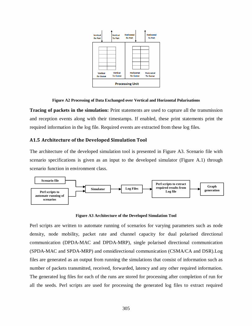
305

Figure A2 Processing of Data Exchanged over Vertical and Horizontal Polarisations

Tracing of packets in the simulation: Print statements are used to capture all the transmission

and reception events along with their timestamps. If enabled, these print statements print the

required information in the log file. Required events are extracted from these log files.

A1.5 Architecture of the Developed Simulation Tool

The architecture of the developed simulation tool is presented in Figure A3. Scenario file with

scenario specifications is given as an input to the developed simulator (Figure A.1) through

scenario function in environment class.

Figure A3 Architecture of the Developed Simulation Tool

Perl scripts are written to automate running of scenarios for varying parameters such as node

density, node mobility, packet rate and channel capacity for dual polarised directional

communication (DPDA-MAC and DPDA-MRP), single polarised directional communication

(SPDA-MAC and SPDA-MRP) and omnidirectional communication (CSMA/CA and DSR).Log

files are generated as an output from running the simulations that consist of information such as

number of packets transmitted, received, forwarded, latency and any other required information.

The generated log files for each of the runs are stored for processing after completion of run for

all the seeds. Perl scripts are used for processing the generated log files to extract required

Scenario file

Simulator Log Files Perl scripts to extract required results from

Log file Graph

generation Perl scripts to automate running of

scenarios

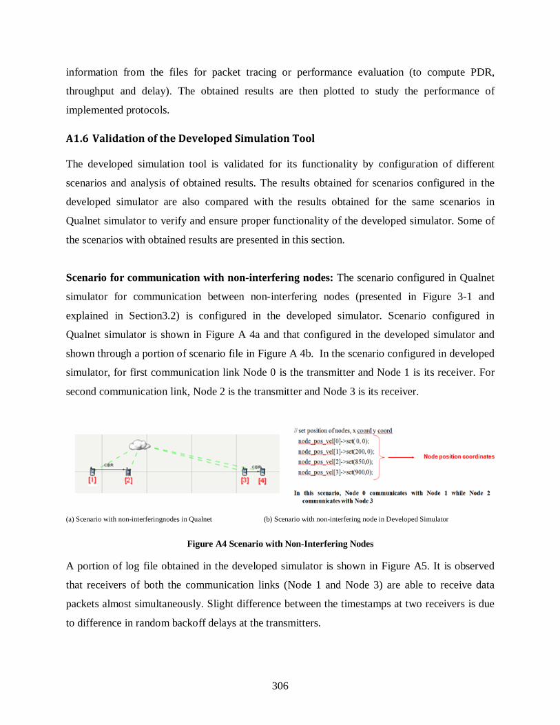
306

information from the files for packet tracing or performance evaluation (to compute PDR,

throughput and delay). The obtained results are then plotted to study the performance of

implemented protocols.

A1.6 Validation of the Developed Simulation Tool

The developed simulation tool is validated for its functionality by configuration of different

scenarios and analysis of obtained results. The results obtained for scenarios configured in the

developed simulator are also compared with the results obtained for the same scenarios in

Qualnet simulator to verify and ensure proper functionality of the developed simulator. Some of

the scenarios with obtained results are presented in this section.

Scenario for communication with non-interfering nodes: The scenario configured in Qualnet

simulator for communication between non-interfering nodes (presented in Figure 3-1 and

explained in Section3.2) is configured in the developed simulator. Scenario configured in

Qualnet simulator is shown in Figure A 4a and that configured in the developed simulator and

shown through a portion of scenario file in Figure A 4b. In the scenario configured in developed

simulator, for first communication link Node 0 is the transmitter and Node 1 is its receiver. For

second communication link, Node 2 is the transmitter and Node 3 is its receiver.

(a) Scenario with non-interferingnodes in Qualnet (b) Scenario with non-interfering node in Developed Simulator

Figure A4 Scenario with Non-Interfering Nodes

A portion of log file obtained in the developed simulator is shown in Figure A5. It is observed

that receivers of both the communication links (Node 1 and Node 3) are able to receive data

packets almost simultaneously. Slight difference between the timestamps at two receivers is due

to difference in random backoff delays at the transmitters.

307

Figure A5 Portion of Log File for Scenario with Non-Interfering Nodes

(a) Packets Transmitted in Qualnet (b) Packets Transmitted in Developed Simulator

Figure A6 Number of Packets Transmitted with Non-Interfering Nodes

Comparison of results obtained for this scenario in Qualnet simulator and in the developed

simulator is shown in Figure A6 and Figure A7. The graph for packets transmitted in Qualnet

(Figure A6 a) is also presented in Figure 3-3 a, and graph for packets received in Qualnet (Figure

A6 b) is also presented in Figure 3-3 b.

Since receiver of first communication link is out of the interference range of transmitter of

second communication link, receivers in both the communication links receive packets

transmitted by their respective transmitters. As seen from Figure A6 and Figure A 7, the results

obtained with developed simulator are same as those obtained with Qualnet simulator.

308

(a) Packets Received in Qualnet (b) Packets Received in Developed Simulator

Figure A7 Number of Packets Transmitted with Non-Interfering Nodes

Scenario for communication with interfering nodes: The scenario for non-interfering node is

modified such that the receiver of first communication link is within interference range of

transmitter of the second communication link.

(a) Scenario with interferingnodes in Qualnet (b) Scenario with interfering node in Developed Simulator

Figure A8 Scenario with Interfering Nodes

This scenario is configured in Qualnet simulator and in the developed simulator. The scenario

configured in Qualnet (Figure A8a) is same as that presented in Figure 3-4 and explained in

Section 3.2. Similar scenario is configured in the developed simulator and shown through a

portion of scenario file in Figure A8b. For the scenario configured in developed simulator, Node

0 is the transmitter and Node 1 is its receiver for first communication link while Node 2 is the

transmitter and Node 3 is its receiver for second communication link. Node 1 and Node 2 are

309

placed within interference range of each other. The portions of DATA and CTS logs (obtained

from the developed simulator) are presented in Figure A9a and Figure A9b respectively. From

the logs it is seen that only Node 3 is able to receive data. This is because Node 1 drops RTS due

interference by Node 2. Therefore, no further exchange of information takes place between Node

0 and Node 1. Result for number of packets transmitted with non-interfering nodes is same as

that for the scenario with interfering nodes (Figure A6) as transmitters of both the

communication links transmit without interference (because they are not within interference

range of each other). However, only the receiver of second communication link is able to receive

the packets from its corresponding transmitter.

(a) DATA Log (b) CTS Log

Figure A 9 Portion of Log Files for Scenario with Interfering Nodes

(a) Packets Received in Qualnet (b) Packets Received in Developed Simulator

Figure A 10 Number of Packets Received with Interfering Nodes

310

A comparison of results obtained for the scenario with interfering nodes in Qualnet simulator and

in the developed simulator is shown in Figure A 10.The graph for packets received in Qualnet

(Figure A 10 a) is also presented in Figure 3-6 b. It is seen that results obtained with the

developed simulator are same as those obtained with Qualnet.

Operation of the developed simulator to support dual polarised directional communication is also

validated through scenarios presented in Section 6.4 of Chapter 6. The developed scenarios along

with their time line values (presented in Figure 6-14 to Figure 6-25) validate the capability of the

nodes to simultaneously communicate over orthogonal polarisations.

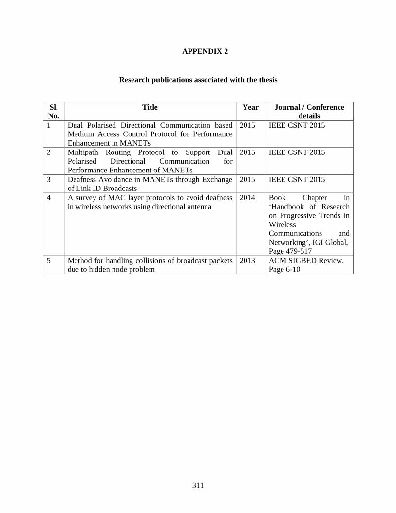
311

APPENDIX 2

Research publications associated with the thesis

Sl. No.

Title Year Journal / Conference details

1 Dual Polarised Directional Communication based Medium Access Control Protocol for Performance Enhancement in MANETs

2015 IEEE CSNT 2015

2 Multipath Routing Protocol to Support Dual Polarised Directional Communication for Performance Enhancement of MANETs

2015 IEEE CSNT 2015

3 Deafness Avoidance in MANETs through Exchange of Link ID Broadcasts

2015 IEEE CSNT 2015

4 A survey of MAC layer protocols to avoid deafness in wireless networks using directional antenna

2014 Book Chapter in ‘Handbook of Research on Progressive Trends in Wireless Communications and Networking’, IGI Global, Page 479-517

5 Method for handling collisions of broadcast packets due to hidden node problem

2013 ACM SIGBED Review, Page 6-10

312

APPENDIX 3

Low Risk Research Ethics Approval Checklist

Simulation Studies on Effects of Dual Polarisation and ... · SIMULATION STUDIES ON EFFECTS OF DUAL...

Documents

Transcript of Simulation Studies on Effects of Dual Polarisation and ... · SIMULATION STUDIES ON EFFECTS OF DUAL...