Combined Navier-Stoke/Direct Simulation Monte Carlo Simulation
Upload
horace-deanCategory
view
215download
0
Simulation
Operations -- Prof. Juran
Operations -- Prof. Juran 2
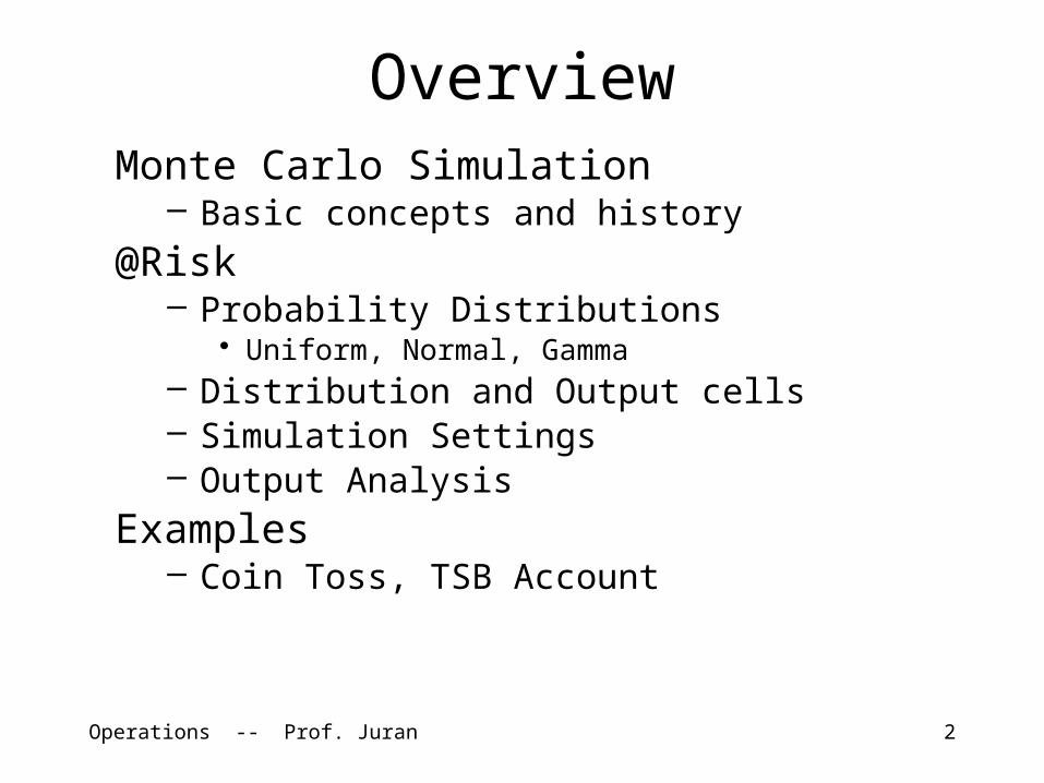
OverviewMonte Carlo Simulation
– Basic concepts and history
@Risk– Probability Distributions
• Uniform, Normal, Gamma– Distribution and Output cells– Simulation Settings– Output Analysis
Examples– Coin Toss, TSB Account
Operations -- Prof. Juran 3
Monte Carlo Simulation
Using theoretical probability distributions to model real-world situations in which randomness is an important factor.
Differences from other spreadsheet models• No optimal solution• Explicit modeling of random variables in
special cells• Many trials, all with different results• Objective function studied using statistical
inference
Operations -- Prof. Juran 4
Operations -- Prof. Juran 5
Operations -- Prof. Juran 6
Operations -- Prof. Juran 7
Operations -- Prof. Juran 8
Operations -- Prof. Juran 9

Operations -- Prof. Juran 10

Operations -- Prof. Juran 11
Origins of Monte Carlo
Stanislaw M. Ulam (1909 - 1984)
Nicholas Metropolis (1915-1999)

Operations -- Prof. Juran 12
Example: Coin Toss
Imagine a game where you flip a coin once. If you get “heads”, you win $3.00 If you get “tails”, you lose $1.00The coin is not fair; it lands on “heads” 35% of the timeWhat is the expected value of this game?
Operations -- Prof. Juran 13
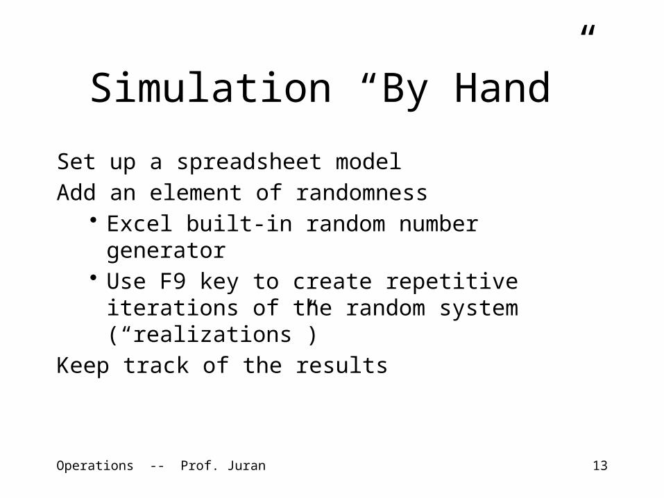
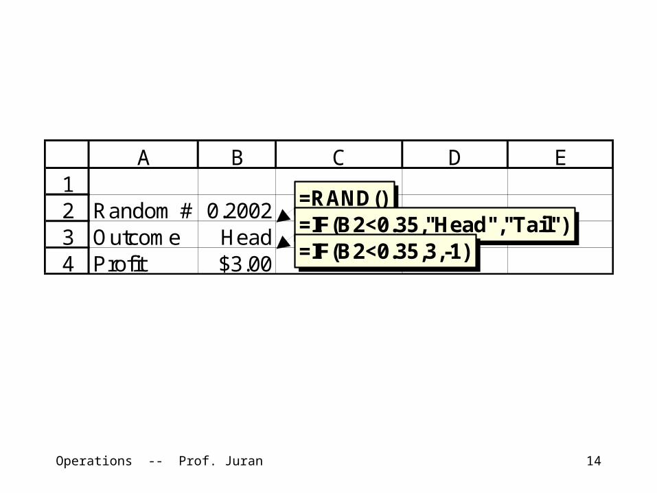
Simulation “By Hand”
Set up a spreadsheet modelAdd an element of randomness
• Excel built-in random number generator• Use F9 key to create repetitive iterations of
the random system (“realizations”)Keep track of the results
Operations -- Prof. Juran 14
1234
A B C D E
Random # 0.2002Outcome HeadProfit $3.00
=RAND()=IF(B2<0.35,"Head","Tail")=IF(B2<0.35,3,-1)
Operations -- Prof. Juran 15
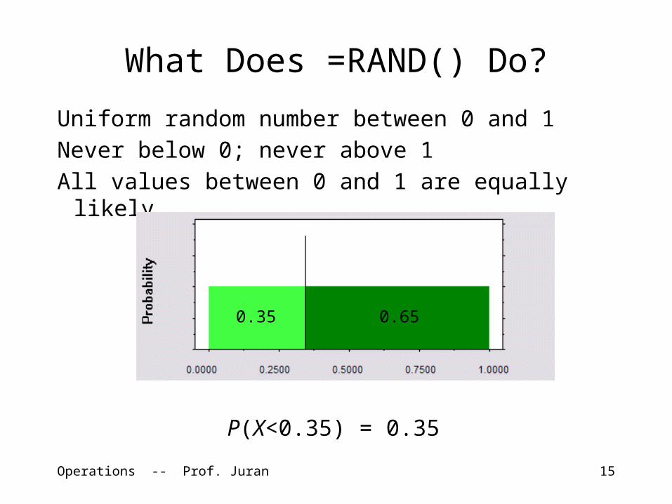
What Does =RAND() Do?
Uniform random number between 0 and 1Never below 0; never above 1All values between 0 and 1 are equally likely
P(X<0.35) = 0.35
0.35 0.65
Operations -- Prof. Juran 16
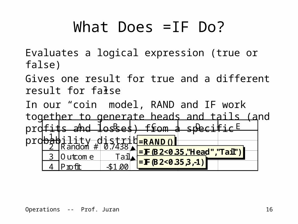
What Does =IF Do?
Evaluates a logical expression (true or false)Gives one result for true and a different result for falseIn our “coin” model, RAND and IF work together to generate heads and tails (and profits and losses) from a specific probability distribution
1234
A B C D E
Random # 0.7438Outcome TailProfit -$1.00
=RAND()=IF(B2<0.35,"Head","Tail")=IF(B2<0.35,3,-1)
Operations -- Prof. Juran 17
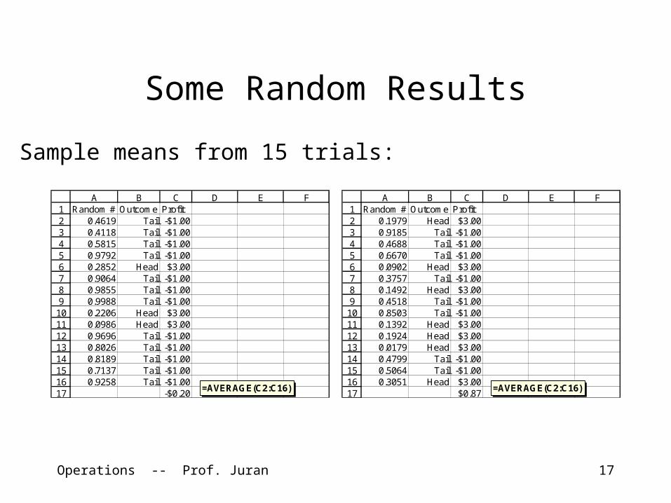
Some Random Results
123456789
1011121314151617
A B C D E FRandom # Outcome Profit
0.4619 Tail -$1.000.4118 Tail -$1.000.5815 Tail -$1.000.9792 Tail -$1.000.2852 Head $3.000.9064 Tail -$1.000.9855 Tail -$1.000.9988 Tail -$1.000.2206 Head $3.000.0986 Head $3.000.9696 Tail -$1.000.8026 Tail -$1.000.8189 Tail -$1.000.7137 Tail -$1.000.9258 Tail -$1.00
-$0.20=AVERAGE(C2:C16)
123456789
1011121314151617
A B C D E FRandom # Outcome Profit
0.1979 Head $3.000.9185 Tail -$1.000.4688 Tail -$1.000.6670 Tail -$1.000.0902 Head $3.000.3757 Tail -$1.000.1492 Head $3.000.4518 Tail -$1.000.8503 Tail -$1.000.1392 Head $3.000.1924 Head $3.000.0179 Head $3.000.4799 Tail -$1.000.5064 Tail -$1.000.3051 Head $3.00
$0.87=AVERAGE(C2:C16)
Sample means from 15 trials:
Operations -- Prof. Juran 18
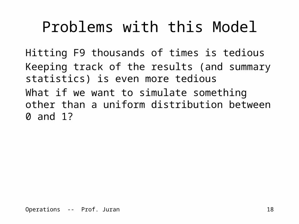
Problems with this Model
Hitting F9 thousands of times is tediousKeeping track of the results (and summary statistics) is even more tediousWhat if we want to simulate something other than a uniform distribution between 0 and 1?
Operations -- Prof. Juran 19
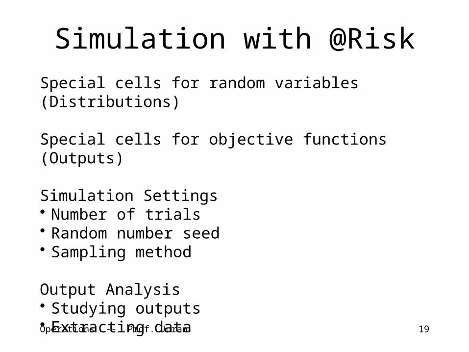
Simulation with @RiskSpecial cells for random variables (Distributions)
Special cells for objective functions (Outputs)
Simulation Settings • Number of trials• Random number seed• Sampling method
Output Analysis• Studying outputs• Extracting data
Operations -- Prof. Juran 20
1234567
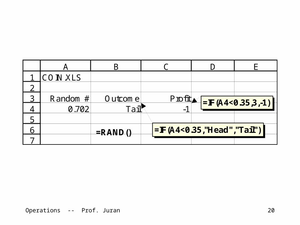
A B C D ECOIN.XLS
Random # Outcome Profit0.702 Tail -1
=RAND() =IF(A4<0.35,"Head","Tail")
=IF(A4<0.35,3,-1)
Operations -- Prof. Juran 21
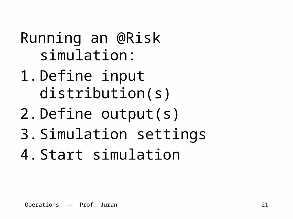
Running an @Risk simulation:1. Define input distribution(s) 2. Define output(s) 3. Simulation settings4. Start simulation
Operations -- Prof. Juran 22
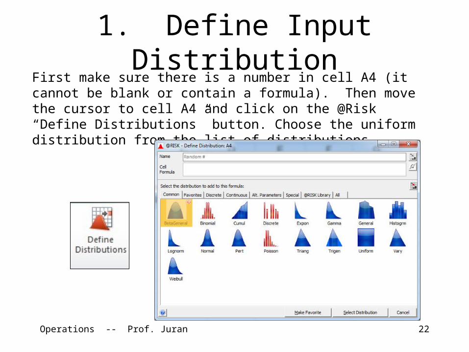
1. Define Input Distribution
First make sure there is a number in cell A4 (it cannot be blank or contain a formula). Then move the cursor to cell A4 and click on the @Risk “Define Distributions” button. Choose the uniform distribution from the list of distributions.
Operations -- Prof. Juran 23
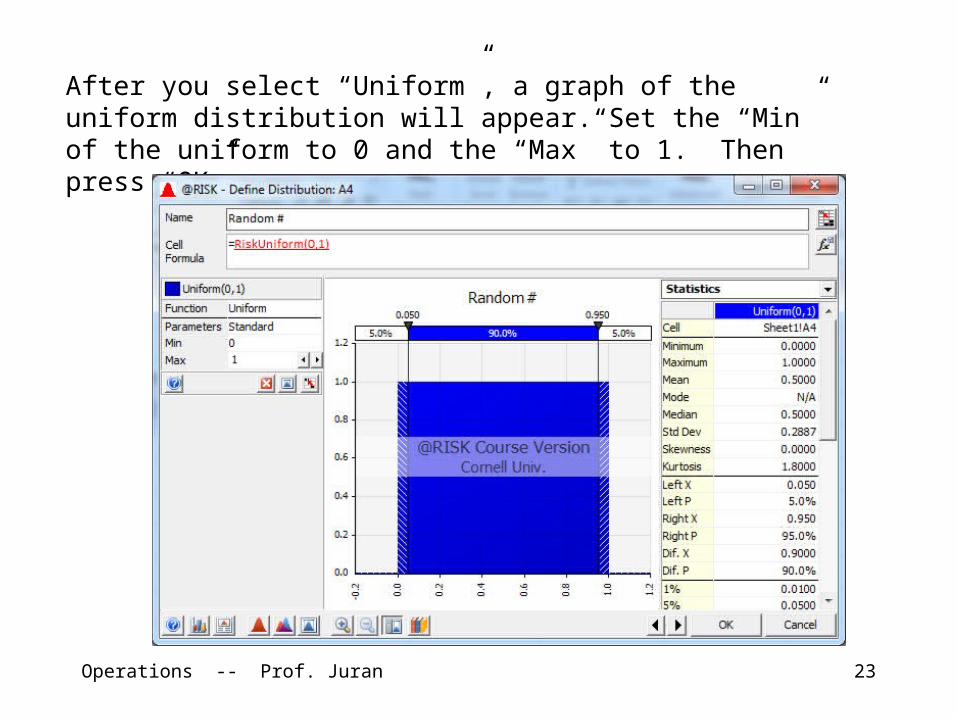
After you select “Uniform”, a graph of the uniform distribution will appear. Set the “Min” of the uniform to 0 and the “Max” to 1. Then press “OK”.
Operations -- Prof. Juran 24
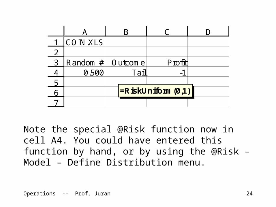
Note the special @Risk function now in cell A4. You could have entered this function by hand, or by using the @Risk – Model – Define Distribution menu.
1234567
A B C DCOIN.XLS
Random # Outcome Profit0.500 Tail -1
=RiskUniform(0,1)
Operations -- Prof. Juran 25
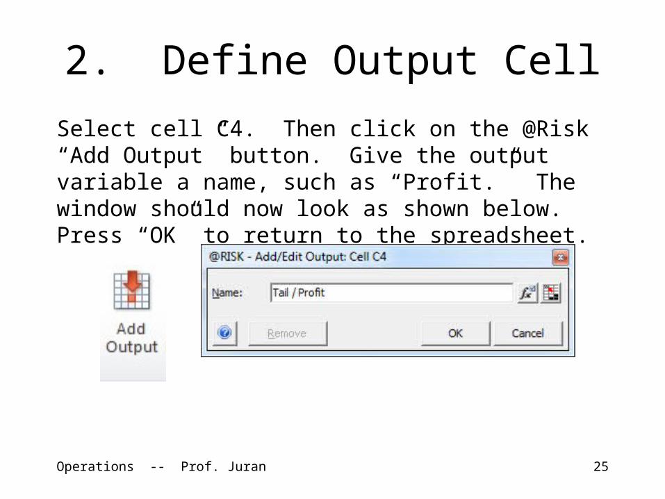
2. Define Output Cell
Select cell C4. Then click on the @Risk “Add Output” button. Give the output variable a name, such as “Profit.” The window should now look as shown below. Press “OK” to return to the spreadsheet.
Operations -- Prof. Juran 26
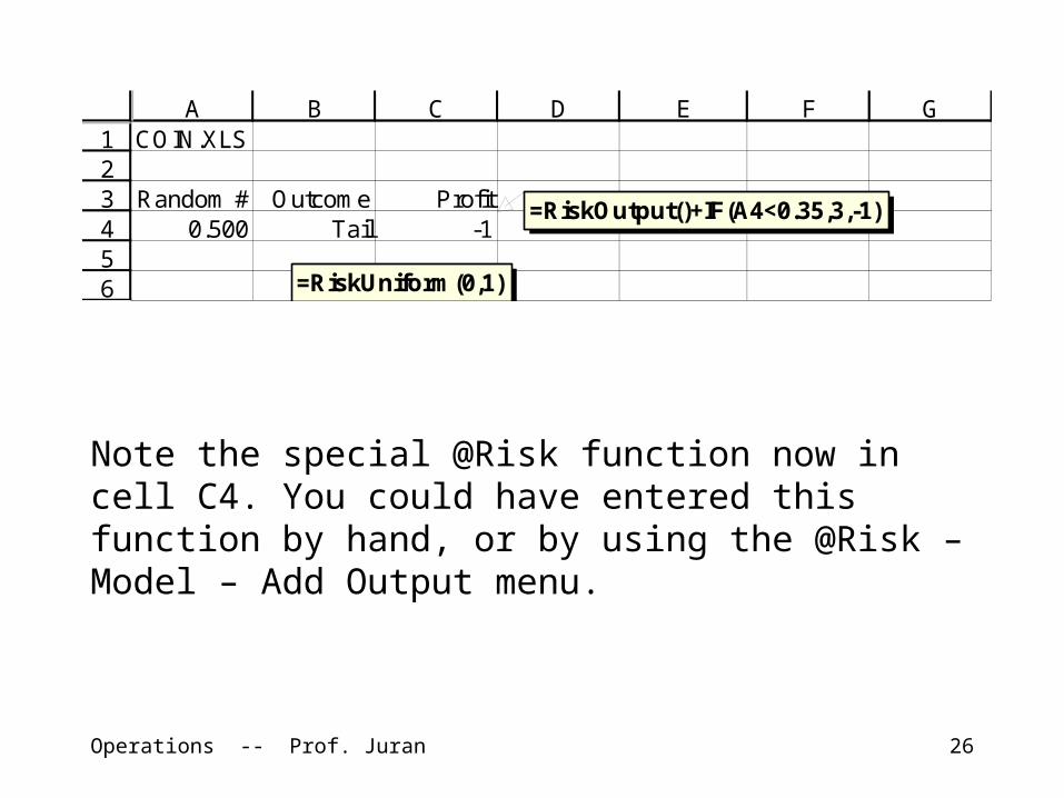
Note the special @Risk function now in cell C4. You could have entered this function by hand, or by using the @Risk – Model – Add Output menu.
123456
A B C D E F GCOIN.XLS
Random # Outcome Profit0.500 Tail -1
=RiskUniform(0,1)
=RiskOutput()+IF(A4<0.35,3,-1)
Operations -- Prof. Juran 27
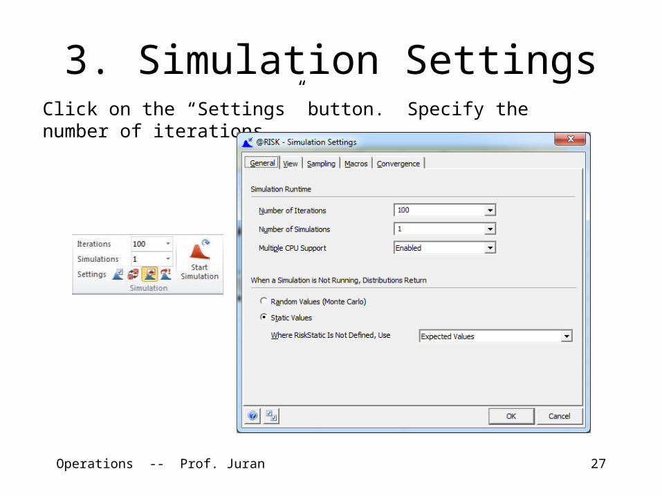
3. Simulation SettingsClick on the “Settings” button. Specify the number of iterations.
Operations -- Prof. Juran 28
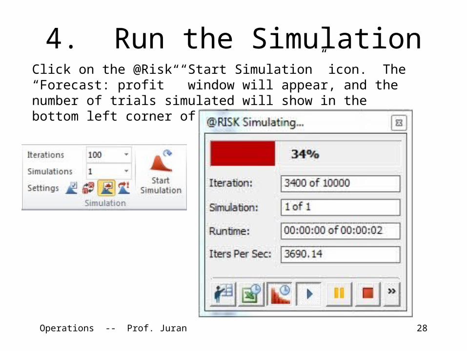
4. Run the SimulationClick on the @Risk “Start Simulation” icon. The “Forecast: profit” window will appear, and the number of trials simulated will show in the bottom left corner of the Excel window.
Operations -- Prof. Juran 29
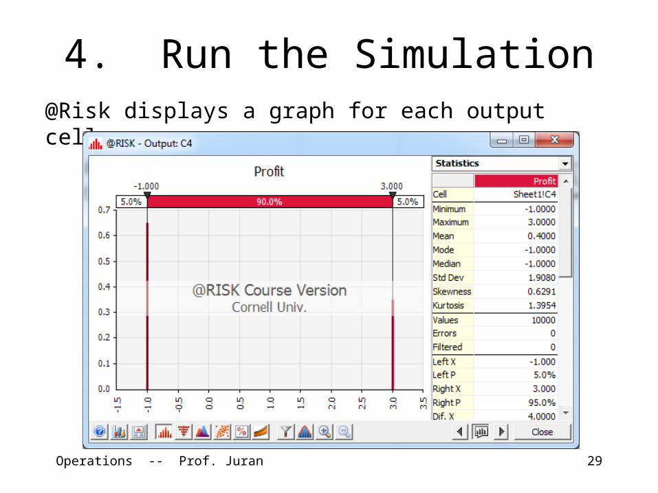
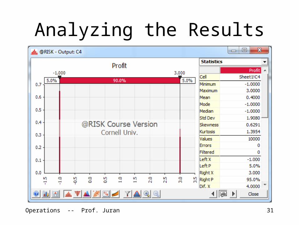
4. Run the Simulation@Risk displays a graph for each output cell.
Operations -- Prof. Juran 30
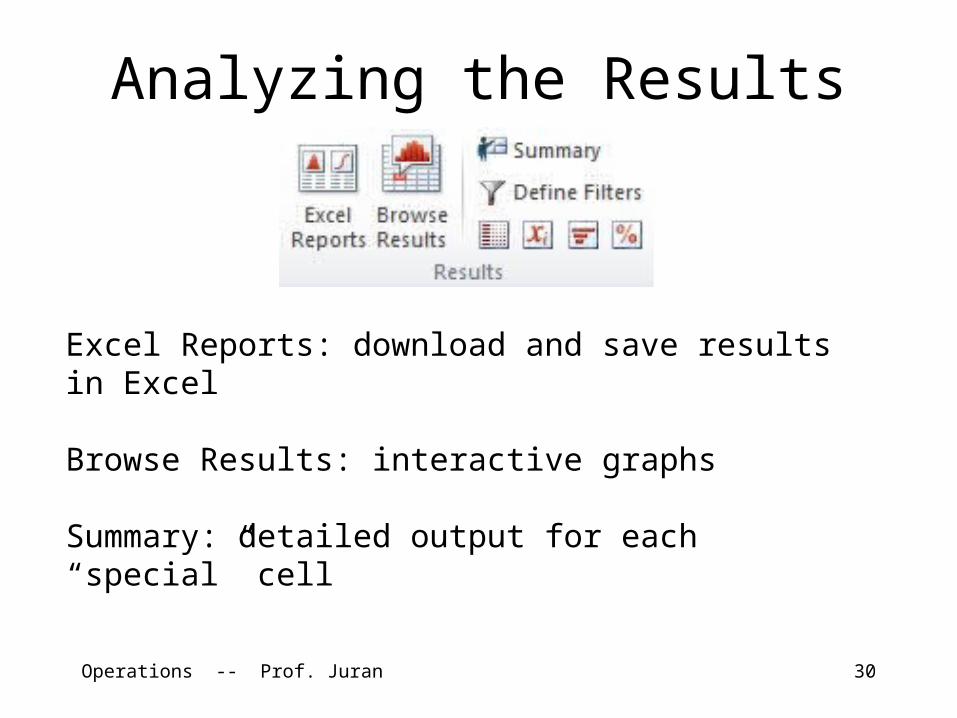
Analyzing the Results
Excel Reports: download and save results in Excel
Browse Results: interactive graphs
Summary: detailed output for each “special” cell
Operations -- Prof. Juran 31
Analyzing the Results
Operations -- Prof. Juran 32
Simulation Results
The 10,000-trial @Risk simulation gives sample mean profit of $0.400. The number $0.400 is only an estimate of the true mean profit from the coin-flipping game.
The standard error of the mean is 0.01908. 𝑠𝑋ത = 𝑠𝑥ξ𝑛
= 1.908ξ10,000
= 0.01908
Operations -- Prof. Juran 33
Simulation ResultsA 95% confidence interval for the true mean profit is approximately:
0.400 1.96(0.01908)
We are 95% confident that the true mean lies somewhere between $0.3626 and $0.4374.
To get a better estimate using simulation, we could increase the number of simulation trials, and continue the simulation run.
Operations -- Prof. Juran 34
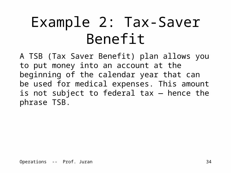
Example 2: Tax-Saver Benefit
A TSB (Tax Saver Benefit) plan allows you to put money into an account at the beginning of the calendar year that can be used for medical expenses. This amount is not subject to federal tax — hence the phrase TSB.
Operations -- Prof. Juran 35
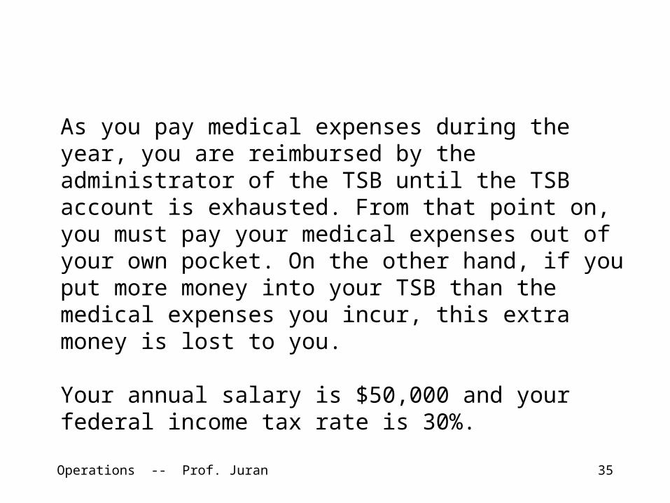
As you pay medical expenses during the year, you are reimbursed by the administrator of the TSB until the TSB account is exhausted. From that point on, you must pay your medical expenses out of your own pocket. On the other hand, if you put more money into your TSB than the medical expenses you incur, this extra money is lost to you.
Your annual salary is $50,000 and your federal income tax rate is 30%.
Operations -- Prof. Juran 36
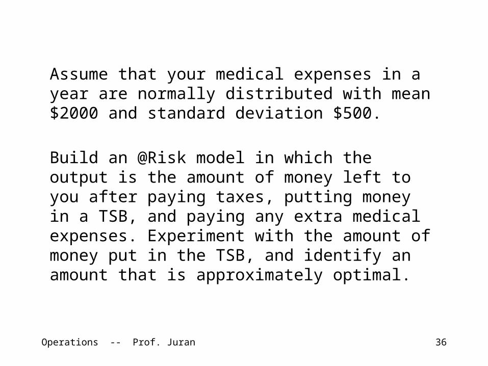
Assume that your medical expenses in a year are normally distributed with mean $2000 and standard deviation $500.
Build an @Risk model in which the output is the amount of money left to you after paying taxes, putting money in a TSB, and paying any extra medical expenses. Experiment with the amount of money put in the TSB, and identify an amount that is approximately optimal.
Operations -- Prof. Juran 37
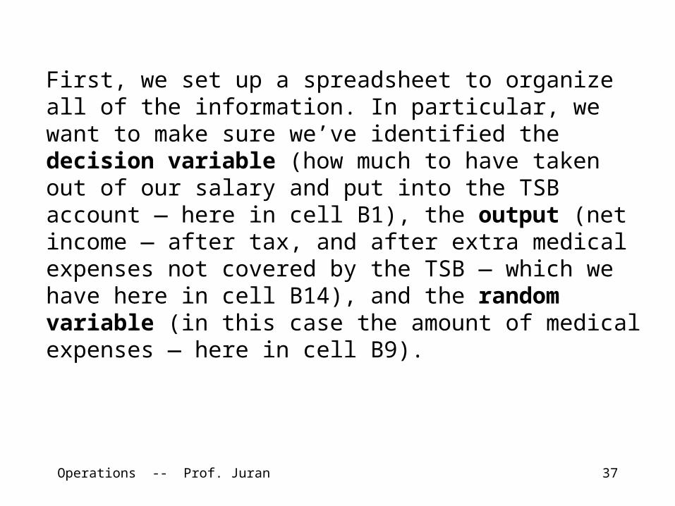
First, we set up a spreadsheet to organize all of the information. In particular, we want to make sure we’ve identified the decision variable (how much to have taken out of our salary and put into the TSB account — here in cell B1), the output (net income — after tax, and after extra medical expenses not covered by the TSB — which we have here in cell B14), and the random variable (in this case the amount of medical expenses — here in cell B9).
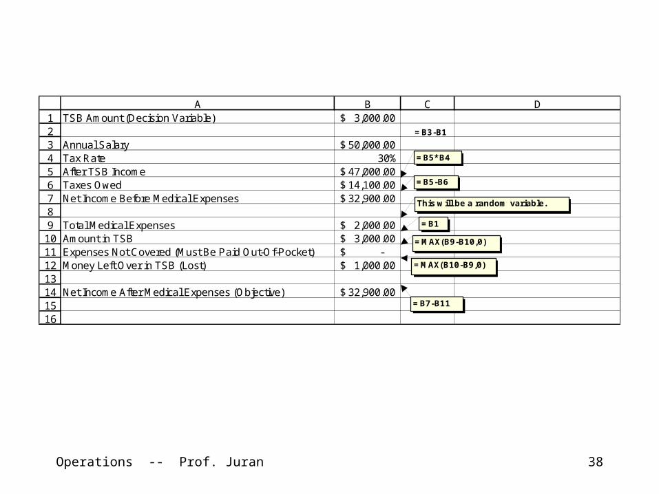
Operations -- Prof. Juran 38
12345678910111213141516
A B C DTSB Amount (Decision Variable) 3,000.00$
Annual Salary 50,000.00$ Tax Rate 30%After TSB Income 47,000.00$ Taxes Owed 14,100.00$ Net Income Before Medical Expenses 32,900.00$
Total Medical Expenses 2,000.00$ Amount in TSB 3,000.00$ Expenses Not Covered (Must Be Paid Out-Of-Pocket) -$ Money Left Over in TSB (Lost) 1,000.00$
Net Income After Medical Expenses (Objective) 32,900.00$
=B3-B1
=B5*B4
=B5-B6
This will be a random variable.
=B1
=MAX(B9-B10,0)
=MAX(B10-B9,0)
=B7-B11
Operations -- Prof. Juran 39
Note (this is important): We will never get a simulation model to tell us directly what is the optimal value of the decision variable (how much to have deducted from our pre-tax pay).
We will try different values (here we have arbitrarily started with $3000 in cell B1) and see how the objective changes.
Through educated trial-and-error, we will eventually come to some conclusion about what is the best amount of money to put into the TSB account.
Operations -- Prof. Juran 40
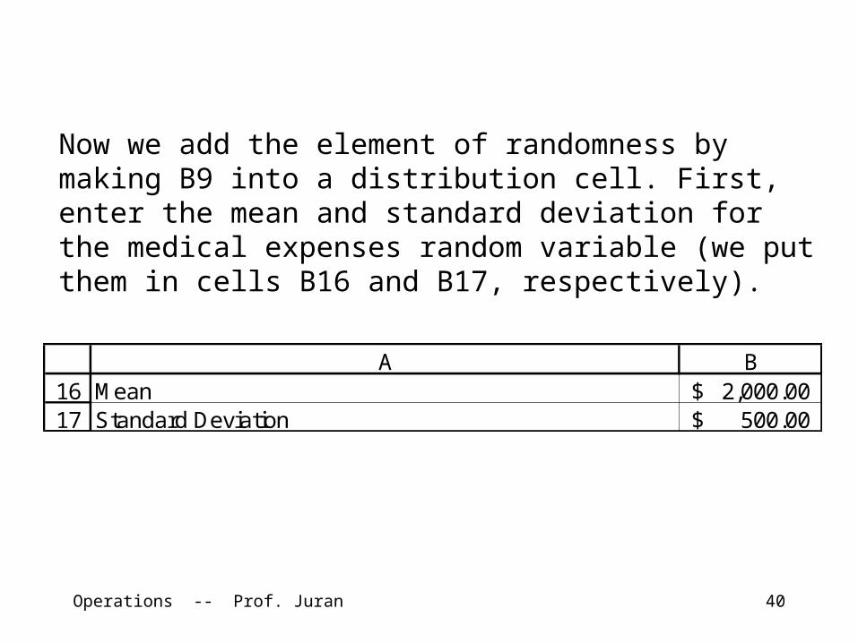
Now we add the element of randomness by making B9 into a distribution cell. First, enter the mean and standard deviation for the medical expenses random variable (we put them in cells B16 and B17, respectively).
1617
A BMean 2,000.00$ Standard Deviation 500.00$
Operations -- Prof. Juran 41
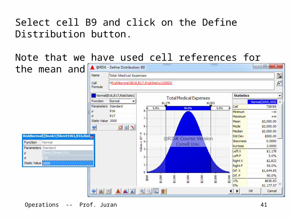
Select cell B9 and click on the Define Distribution button.
Note that we have used cell references for the mean and standard deviation.
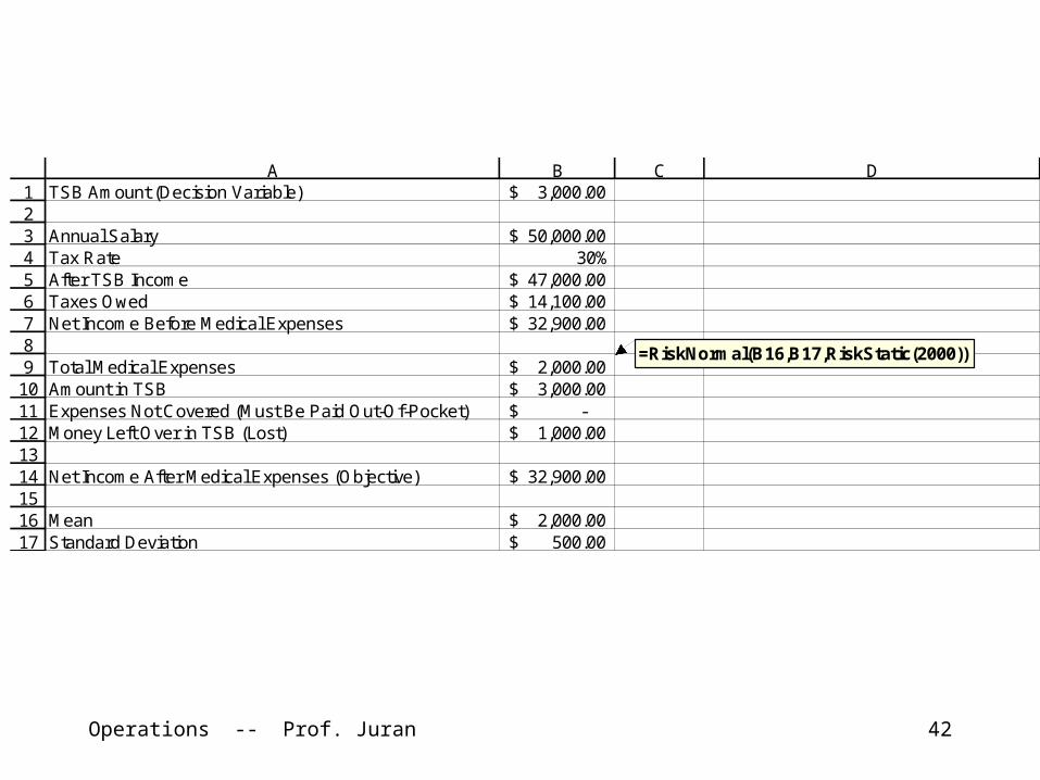
Operations -- Prof. Juran 42
1234567891011121314151617
A B C DTSB Amount (Decision Variable) 3,000.00$
Annual Salary 50,000.00$ Tax Rate 30%After TSB Income 47,000.00$ Taxes Owed 14,100.00$ Net Income Before Medical Expenses 32,900.00$
Total Medical Expenses 2,000.00$ Amount in TSB 3,000.00$ Expenses Not Covered (Must Be Paid Out-Of-Pocket) -$ Money Left Over in TSB (Lost) 1,000.00$
Net Income After Medical Expenses (Objective) 32,900.00$
Mean 2,000.00$ Standard Deviation 500.00$
=RiskNormal(B16,B17,RiskStatic(2000))
Operations -- Prof. Juran 43
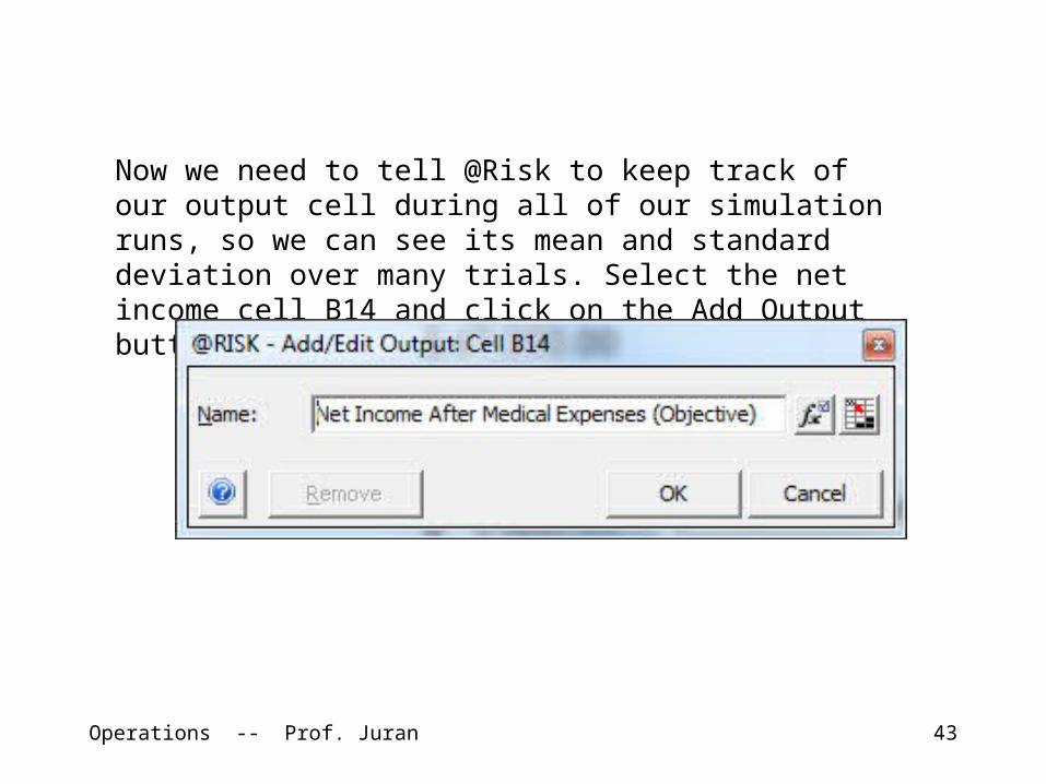
Now we need to tell @Risk to keep track of our output cell during all of our simulation runs, so we can see its mean and standard deviation over many trials. Select the net income cell B14 and click on the Add Output button.
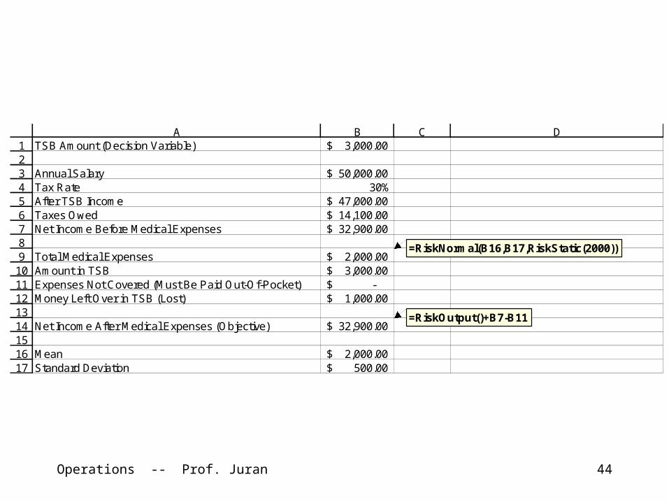
Operations -- Prof. Juran 44
123456789
1011121314151617
A B C DTSB Amount (Decision Variable) 3,000.00$
Annual Salary 50,000.00$ Tax Rate 30%After TSB Income 47,000.00$ Taxes Owed 14,100.00$ Net Income Before Medical Expenses 32,900.00$
Total Medical Expenses 2,000.00$ Amount in TSB 3,000.00$ Expenses Not Covered (Must Be Paid Out-Of-Pocket) -$ Money Left Over in TSB (Lost) 1,000.00$
Net Income After Medical Expenses (Objective) 32,900.00$
Mean 2,000.00$ Standard Deviation 500.00$
=RiskNormal(B16,B17,RiskStatic(2000))
=RiskOutput()+B7-B11
Operations -- Prof. Juran 45
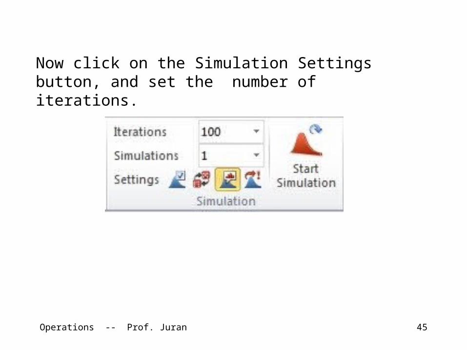
Now click on the Simulation Settings button, and set the number of iterations.
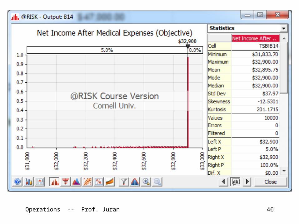
Operations -- Prof. Juran 46
Operations -- Prof. Juran 47
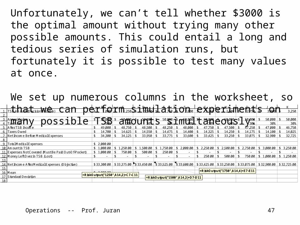
Unfortunately, we can’t tell whether $3000 is the optimal amount without trying many other possible amounts. This could entail a long and tedious series of simulation runs, but fortunately it is possible to test many values at once.
We set up numerous columns in the worksheet, so that we can perform simulation experiments on many possible TSB amounts simultaneously:1
23456789101112131415161718
A B C D E F G H I J KTSB Amount (Decision Variable) 1,000$ 1,250$ 1,500$ 1,750$ 2,000$ 2,250$ 2,500$ 2,750$ 3,000$ 3,250$
Annual Salary 50,000$ 50,000$ 50,000$ 50,000$ 50,000$ 50,000$ 50,000$ 50,000$ 50,000$ 50,000$ Tax Rate 30% 30% 30% 30% 30% 30% 30% 30% 30% 30%After TSB Income 49,000$ 48,750$ 48,500$ 48,250$ 48,000$ 47,750$ 47,500$ 47,250$ 47,000$ 46,750$ Taxes Owed 14,700$ 14,625$ 14,550$ 14,475$ 14,400$ 14,325$ 14,250$ 14,175$ 14,100$ 14,025$ Net Income Before Medical Expenses 34,300$ 34,125$ 33,950$ 33,775$ 33,600$ 33,425$ 33,250$ 33,075$ 32,900$ 32,725$
Total Medical Expenses 2,000.00$ Amount in TSB 1,000.00$ 1,250.00$ 1,500.00$ 1,750.00$ 2,000.00$ 2,250.00$ 2,500.00$ 2,750.00$ 3,000.00$ 3,250.00$ Expenses Not Covered (Must Be Paid Out-Of-Pocket) 1,000.00$ 750.00$ 500.00$ 250.00$ -$ -$ -$ -$ -$ -$ Money Left Over in TSB (Lost) -$ -$ -$ -$ -$ 250.00$ 500.00$ 750.00$ 1,000.00$ 1,250.00$
Net Income After Medical Expenses (Objective) 33,300.00$ 33,375.00$ 33,450.00$ 33,525.00$ 33,600.00$ 33,425.00$ 33,250.00$ 33,075.00$ 32,900.00$ 32,725.00$
Mean 2,000.00$ Standard Deviation 500.00$ =RiskOutput("1250",A14,2)+C7-C11
=RiskOutput("1500",A14,3)+D7-D11
=RiskOutput("1750",A14,4)+E7-E11
Operations -- Prof. Juran 48
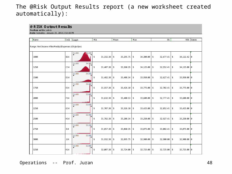
The @Risk Output Results report (a new worksheet created automatically):
@RISK Output ResultsPerformed By: adminDate: Saturday, J anuary 25, 2014 2:54:48 PM
Name Cell Graph Min Mean Max 5% 95% Errors
Range: Net Income After Medical Expenses (Objective)
1000 B14 $ 31,332.38 $ 33,295.75 $ 34,300.00 $ 32,477.41 $ 34,122.42 0
1250 C14 $ 31,407.38 $ 33,360.35 $ 34,125.00 $ 32,552.41 $ 34,125.00 0
1500 D14 $ 31,482.38 $ 33,408.34 $ 33,950.00 $ 32,627.41 $ 33,950.00 0
1750 E14 $ 31,557.38 $ 33,426.10 $ 33,775.00 $ 32,702.41 $ 33,775.00 0
2000 F14 $ 31,632.38 $ 33,400.53 $ 33,600.00 $ 32,777.41 $ 33,600.00 0
2250 G14 $ 31,707.38 $ 33,326.10 $ 33,425.00 $ 32,852.41 $ 33,425.00 0
2500 H14 $ 31,782.38 $ 33,208.34 $ 33,250.00 $ 32,927.41 $ 33,250.00 0
2750 I14 $ 31,857.38 $ 33,060.35 $ 33,075.00 $ 33,002.41 $ 33,075.00 0
3000 J 14 $ 31,932.38 $ 32,895.75 $ 32,900.00 $ 32,900.00 $ 32,900.00 0
3250 K14 $ 32,007.38 $ 32,724.00 $ 32,725.00 $ 32,725.00 $ 32,725.00 0
Operations -- Prof. Juran 49
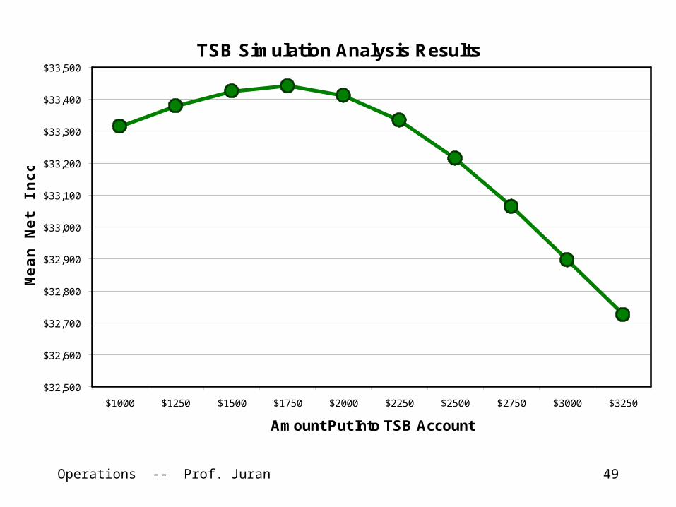
TSB Simulation Analysis Results
$32,500
$32,600
$32,700
$32,800
$32,900
$33,000
$33,100
$33,200
$33,300
$33,400
$33,500
$1000 $1250 $1500 $1750 $2000 $2250 $2500 $2750 $3000 $3250
Amount Put Into TSB Account
Me
an
Ne
t In
co
me
Operations -- Prof. Juran 50
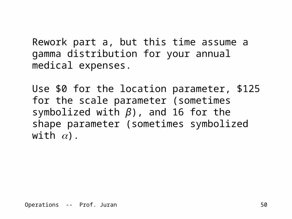
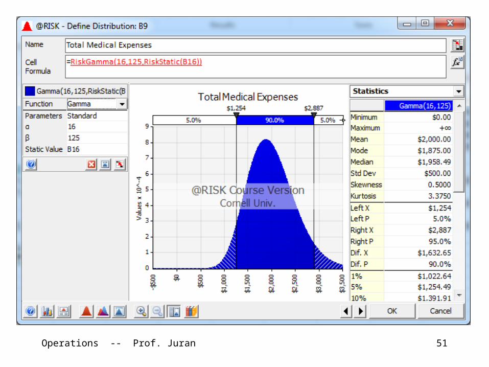
Rework part a, but this time assume a gamma distribution for your annual medical expenses.
Use $0 for the location parameter, $125 for the scale parameter (sometimes symbolized with β), and 16 for the shape parameter (sometimes symbolized with ).
Operations -- Prof. Juran 51
Operations -- Prof. Juran 52
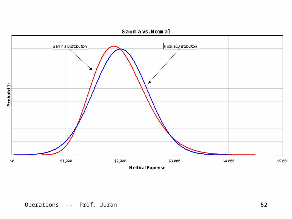
Gamma vs. Normal
$0 $1,000 $2,000 $3,000 $4,000 $5,000
Medical Expense
Pro
ba
bili
ty
Gamma Distribution Normal Distribution
Operations -- Prof. Juran 53
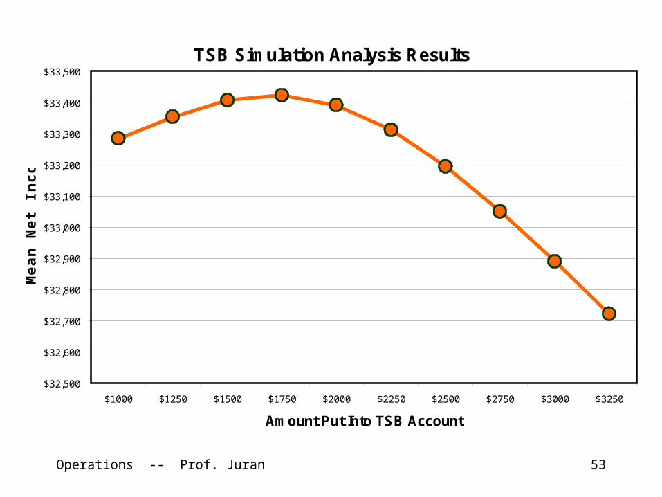
TSB Simulation Analysis Results
$32,500
$32,600
$32,700
$32,800
$32,900
$33,000
$33,100
$33,200
$33,300
$33,400
$33,500
$1000 $1250 $1500 $1750 $2000 $2250 $2500 $2750 $3000 $3250
Amount Put Into TSB Account
Me
an
Ne
t In
co
me
Operations -- Prof. Juran 54
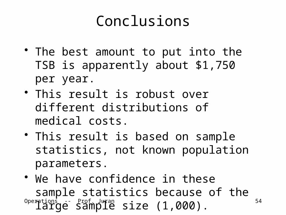
Conclusions
• The best amount to put into the TSB is apparently about $1,750 per year.
• This result is robust over different distributions of medical costs.
• This result is based on sample statistics, not known population parameters.
• We have confidence in these sample statistics because of the large sample size (1,000).
Operations -- Prof. Juran 55
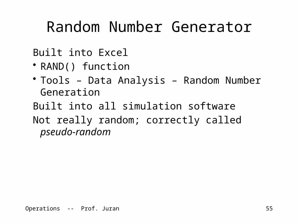
Built into Excel• RAND() function• Tools – Data Analysis – Random Number
GenerationBuilt into all simulation softwareNot really random; correctly called pseudo-random
Random Number Generator
Operations -- Prof. Juran 56
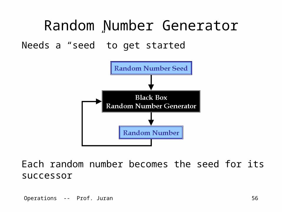
Needs a “seed” to get started
Each random number becomes the seed for its successor
Random Number Generator
Operations -- Prof. Juran 57
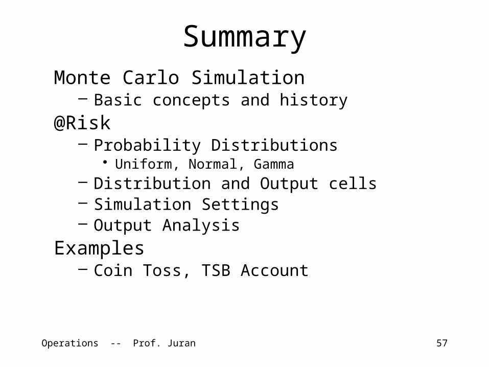
SummaryMonte Carlo Simulation
– Basic concepts and history
@Risk– Probability Distributions
• Uniform, Normal, Gamma– Distribution and Output cells– Simulation Settings– Output Analysis
Examples– Coin Toss, TSB Account