Simulation of Sliding Wear

Tribology International 32 (1999) 71–81www.elsevier.com/locate/triboint

Simulating sliding wear with finite element method

Priit Podra a,*, Soren Anderssonb

a Department of Machine Science, Tallinn Technical University, TTU, Ehitajate tee 5, 19086 Tallinn, Estoniab Machine Elements, Department of Machine Design, Royal Institute of Technology, KTH, S-100 44 Stockholm, Sweden

Received 5 September 1997; received in revised form 18 January 1999; accepted 25 March 1999

Abstract

Wear of components is often a critical factor influencing the product service life. Wear prediction is therefore an important partof engineering. The wear simulation approach with commercial finite element (FE) software ANSYS is presented in this paper. Amodelling and simulation procedure is proposed and used with the linear wear law and the Euler integration scheme. Good care,however, must be taken to assure model validity and numerical solution convergence. A spherical pin-on-disc unlubricated steelcontact was analysed both experimentally and with FEM, and the Lim and Ashby wear map was used to identify the wear mech-anism. It was shown that the FEA wear simulation results of a given geometry and loading can be treated on the basis of wearcoefficient2sliding distance change equivalence. The finite element software ANSYS is well suited for the solving of contactproblems as well as the wear simulation. The actual scatter of the wear coefficient being within the limits of±40–60% led toconsiderable deviation of wear simulation results. These results must therefore be evaluated on a relative scale to compare differentdesign options. 1999 Elsevier Science Ltd. All rights reserved.

Keywords:Wear simulation; FEA; Wear tests; Contact temperature

1. Introduction

The most confident knowledge about the friction pairtribological behaviour can be achieved by making wearexperiments. However, the particular design alternativesneed to be evaluated quickly on a regular in-house rou-tine basis. A massive amount of research has been car-ried out to help designers with that respect.

It has been argued that the dominating parameterscontributing to the sliding wear of a given system arethe loading and the relative sliding of the contact. Thevelocity is determined by the mechanism kinematics.The question of how the system load influences theactual contact stress field is more complicated. The firstrelevant analysis of the stress at the contact of two elasticsolids was presented by Hertz. He regarded the con-tacting bodies as elastic half-spaces and the contactbetween them ellipse-shaped, frictionless and non-con-

* Corresponding author. Tel.:+372-620-33-02; fax:+372-620-31-96.

E-mail addresses: [email protected] (P. Po˜dra), [email protected] (S. Andersson)

0301-679X/99/$ - see front matter. 1999 Elsevier Science Ltd. All rights reserved.PII: S0301-679X(99 )00012-2

forming. This approach has often been used in the con-tact stress calculations.

Wear takes place when surfaces of mechanicalcomponents contact each other. The question of greatpractical importance is, how much of the material willbe lost during the given operation time. The surfaceshapes vary due to their functions, manufacturing toler-ances, etc. and will be changed as a result of wear andplastic deformation. The pressure distribution is thenstrongly dependent on those phenomena. A finiteelement method (FEM) is a versatile tool to solve thestress and strain problems regardless of the geometry ofthe bodies. A FEA program ANSYS 5.0A has been usedin this paper for the contact pressure determination aswell as wear simulation.

2. Wear models

The wear process can be treated as a dynamic process,depending on many parameters and the prediction of thatprocess as an initial value problem. The wear rate maythen be described by a general equation

72 P. Podra, S. Andersson / Tribology International 32 (1999) 71–81

Nomenclature

A apparent contact area (m2)a0 thermal diffusivity (m2/s)D stiffness (N/m)E elastic modulus (Pa)E* normalised elastic modulus (Pa)fFr friction coefficientF load (N)FN normal load (N)H hardness (Pa)HV Vickers hardness (Pa)h wear depth (m)k dimensional wear coefficient (Pa21)K wear coefficientKm thermal conductivity of steel (J/m/s/K)KN contact stiffness (N/m)M time scale factorp normal contact pressure (Pa)p dimensionless normalised pressurePe Peclet numberq0 heat flux (W/m2)Q dimensionless normalised wear rater0 apparent contact area radius (m)rp pin sliding track average radius (m)R pin tip radius (m)R1 torus profile radius of curvature (m)s sliding distance (m)t time (s)T temperature (K)u Nodal displacement (m)v velocity (m/s)v dimensionless normalised velocityV volume wear (m3)x, y Cartesian coordinates (m)a cone angle (°)a12 heat distribution coefficientD difference, incrementj spinning angle (rad)m Poisson ratio

Subscripts

aver averageContact belongs to contactDisc belongs to discflash flash temperaturei sampling point encounterin initialj solution step encounterlim maximum allowedmax maximumPin belongs to pin

dhds

5f (load, velocity, temperature,

material parameters, lubrication, . . . )

whereh is the wear depth (m) ands is the sliding dis-tance (m). Many wear models are available in the litera-ture. Their mathematical expressions vary from simpleempirical relationships to complicated equations relyingon physical concepts and definitions [1]. Specific par-ameters and variables are often involved, valid only for aparticular case and not available in handbooks. Thereforevery few of those models have been used to predict wearin practice.

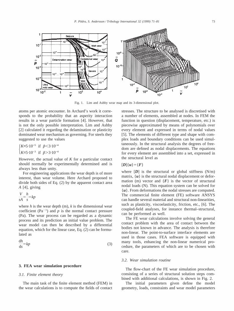
A comprehensive wear classification for steels overthe wide range of loads and sliding velocities was givenby Lim and Ashby [2]. They based their work on simpli-fied wear equations and adjusted them on the basis ofdata from a large number of dry pin-on-disc exper-iments. This work resulted in a wear map, Fig. 1, givingthe contours of wear regimes and the dimensionless wearrateQ as a function of dimensionless normalised press-ure p and dimensionless normalised velocityv, definedas

Q5VAs

, p5FN

AHandv5

vr0

a0

(1)

whereV is the volume wear (m3), A is the apparent con-tact area (m2) and r0 is its radius (m),FN is the normalload (N), H is the hardness (Pa) of softer material incontact,v is the relative sliding velocity (m/s) anda0 isthe material’s thermal diffusivity (m2/s). The wearequations and the parameters used by Lim and Ashbyare shown in Table 1.

The temperature analysis, on which the wear map inFig. 1 was based assumed a simple 1-dimensional heatflow. Further, in the regime in which the flash tempera-tures play an important role on wear, the heat distributioncoefficient was taken to be equal toa12=0.5. If the con-tact flash temperature is above 700°C, the oxidationalwear mechanism will prevail in a steel contact. Belowthis temperature limit, the wear law was proven to belinear with respect to load and independent of velocity.

The most frequently used model is the linear wearequation Q=Kp, where the volume wear rate is pro-portional to the normal load. This model is often referredto as the Archard’s wear law, though its basic form wasfirst published by Holm [3]. The model was based onexperimental observations and written in the form

Vs5K

FN

H(2)

The wear coefficientK was introduced to provideagreement between theory and experiment. Holm treatedit as a constant, representing the number of abraded

73P. Podra, S. Andersson / Tribology International 32 (1999) 71–81

Fig. 1. Lim and Ashby wear map and its 3-dimensional plot.

atoms per atomic encounter. In Archard’s work it corre-sponds to the probability that an asperity interactionresults in a wear particle formation [4]. However, thatis not the only possible interpretation. Lim and Ashby[2] calculated it regarding the delamination or plasticitydominated wear mechanism as governing. For steels theysuggested to use the values

HK=5·10−5 if p,3·10−4

K=5·10−3 if p.3·10−4

However, the actual value ofK for a particular contactshould normally be experimentally determined and isalways less than unity.

For engineering applications the wear depth is of moreinterest, than wear volume. Here Archard proposed todivide both sides of Eq. (2) by the apparent contact areaA [4], giving

VsA

5hs5kp

whereh is the wear depth (m),k is the dimensional wearcoefficient (Pa21) and p is the normal contact pressure(Pa). The wear process can be regarded as a dynamicprocess and its prediction an initial value problem. Thewear model can then be described by a differentialequation, which for the linear case, Eq. (2) can be formu-lated as

dhds

5kp (3)

3. FEA wear simulation procedure

3.1. Finite element theory

The main task of the finite element method (FEM) inthe wear calculations is to compute the fields of contact

stresses. The structure to be analysed is discretised witha number of elements, assembled at nodes. In FEM thefunction in question (displacement, temperature, etc.) ispiecewise approximated by means of polynomials overevery element and expressed in terms of nodal values[5]. The elements of different type and shape with com-plex loads and boundary conditions can be used simul-taneously. In the structural analysis the degrees of free-dom are defined as nodal displacements. The equationsfor every element are assembled into a set, expressed inthe structural level as

[D]{ u} 5{ F}

where [D] is the structural or global stiffness (N/m)matrix, {u} is the structural nodal displacement or defor-mation (m) vector and {F} is the vector of structuralnodal loads (N). This equation system can be solved for{ u}. From deformations the nodal stresses are computed.The commercial finite element (FE) software ANSYScan handle several material and structural non-linearities,such as plasticity, viscoelasticity, friction, etc., [6]. Thecoupled-field analyses, for instance thermal–structural,can be performed as well.

The FE wear calculations involve solving the generalcontact problem with the area of contact between thebodies not known in advance. The analysis is thereforenon-linear. The point-to-surface interface elements areused in those cases. FEA software is equipped withmany tools, enhancing the non-linear numerical pro-cedure, the parameters of which are to be chosen withcare.

3.2. Wear simulation routine

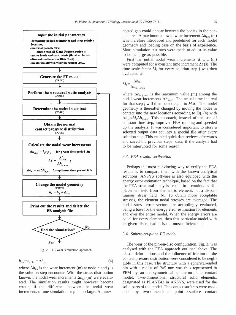
The flow-chart of the FE wear simulation procedure,consisting of a series of structural solution steps com-bined with additional calculations, is shown in Fig. 2.

The initial parameters given define the modelgeometry, loads, constraints and wear model parameters


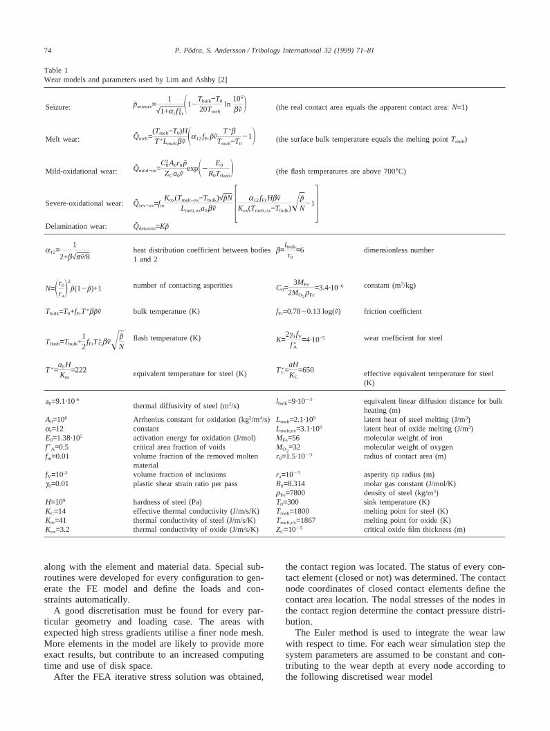
Table 1Wear models and parameters used by Lim and Ashby [2]

pseizure=1

√1+at f2Fr

S12Tbulk−T0

20Tmelt

ln106

bvDSeizure: (the real contact area equals the apparent contact area:N=1)

Qmelt=(Tmelt−T0)HT∗Lmeltbv

Sa12fFrpvT∗b

Tmelt−T0

21DMelt wear: (the surface bulk temperature equals the melting pointTmelt)

Qmild−ox=C2

0A0r0pZCa0v

expS2E0

R0TflashDMild-oxidational wear: (the flash temperatures are above 700°C)

Qsev−ox=fmKox(Tmelt−ox−Tbulk)√pN

Lmelt,oxa0bv 3 a12fFrHbvKox(Tmelt,ox−Tbulk)!

pN

214Severe-oxidational wear:

Delamination wear: Qdelamin=Kp

a12=1

2+b√pv/8b=

lbulk

r0

=6heat distribution coefficient between bodies dimensionless number1 and 2

number of contacting asperities constant (m3/kg)C0=3MFe

2MO2rFe

=3.4·10−6N=Sr0

raD2

p(12p)+1

Tbulk=T0+fFrT∗bpv bulk temperature (K) fFr=0.7820.13 log(v) friction coefficient

flash temperature (K) wear coefficient for steelK=2g0fV

f∗A

=4·10−5Tflash=Tbulk+

12

fFrT∗Cbv! p

N

T∗=a0HKm

=222 T∗C=

aHKC

=650equivalent temperature for steel (K) effective equivalent temperature for steel(K)

a0=9.1·10-6 lbulk=9·1023 equivalent linear diffusion distance for bulkthermal diffusivity of steel (m2/s)

heating (m)A0=106 Arrhenius constant for oxidation (kg2/m4/s) Lmelt=2.1·109 latent heat of steel melting (J/m3)at=12 constant Lmelt,ox=3.1·109 latent heat of oxide melting (J/m3)E0=1.38·105 activation energy for oxidation (J/mol) MFe=56 molecular weight of ironf *

A=0.5 critical area fraction of voids MO2=32 molecular weight of oxygen

fm=0.01 volume fraction of the removed molten r0=1.5·1023 radius of contact area (m)material

fV=10-3 volume fraction of inclusions ra=1025 asperity tip radius (m)g0=0.01 plastic shear strain ratio per pass R0=8.314 molar gas constant (J/mol/K)

rFe=7800 density of steel (kg/m3)H=109 hardness of steel (Pa) T0=300 sink temperature (K)KC=14 effective thermal conductivity (J/m/s/K) Tmelt=1800 melting point for steel (K)Km=41 thermal conductivity of steel (J/m/s/K) Tmelt,ox=1867 melting point for oxide (K)Kox=3.2 thermal conductivity of oxide (J/m/s/K) ZC=1025 critical oxide film thickness (m)

along with the element and material data. Special sub-routines were developed for every configuration to gen-erate the FE model and define the loads and con-straints automatically.

A good discretisation must be found for every par-ticular geometry and loading case. The areas withexpected high stress gradients utilise a finer node mesh.More elements in the model are likely to provide moreexact results, but contribute to an increased computingtime and use of disk space.

After the FEA iterative stress solution was obtained,

the contact region was located. The status of every con-tact element (closed or not) was determined. The contactnode coordinates of closed contact elements define thecontact area location. The nodal stresses of the nodes inthe contact region determine the contact pressure distri-bution.

The Euler method is used to integrate the wear lawwith respect to time. For each wear simulation step thesystem parameters are assumed to be constant and con-tributing to the wear depth at every node according tothe following discretised wear model


Fig. 2. FE wear simulation approach.

hj,n5hj−1,n1Dhj,n (4)

whereDhj,n is the wear increment (m) at noden and j isthe solution step encounter. With the stress distributionknown, the nodal wear incrementsDhj,n (m) were evalu-ated. The simulation results might however becomeerratic, if the difference between the nodal wearincrements of one simulation step is too large. An unex-

pected gap could appear between the bodies in the con-tact area. A maximum allowed wear incrementDhlim (m)was therefore introduced and predefined for each modelgeometry and loading case on the basis of experience.Short simulation test runs were made to adjust its valueto be as large as possible.

First the initial nodal wear incrementsDhin, j,n (m)were computed for a constant time incrementDt (s). Thetime scale factorMj for every solution stepj was thenevaluated as

Mj 5Dhlim

Dhin, j,max

where Dhin,j,max is the maximum value (m) among thenodal wear incrementsDhin,j,n. The actual time intervalfor that stepj will then be set equal toMjDt. The modelgeometry is thereafter changed by moving the nodes incontact into the new locations according to Eq. (4) withDhj,n=Mj Dhin, j,n. This approach, instead of the use ofconstant time step, improved FEA running and speededup the analysis. It was considered important to store aselected output data set into a special file after everysolution step. This enabled quick data reviews afterwardsand saved the previous steps’ data, if the analysis hadto be interrupted for some reason.

3.3. FEA results verification

Perhaps the most convincing way to verify the FEAresults is to compare them with the known analyticalsolutions. ANSYS software is also equipped with theenergy error estimation technique, based on the fact thatthe FEA structural analysis results in a continuous dis-placement field from element to element, but a discon-tinuous stress field [6]. To obtain more acceptablestresses, the element nodal stresses are averaged. Thenodal stress error vectors are accordingly evaluated,being a base for the energy error estimation for elementsand over the entire model. When the energy errors areequal for every element, then that particular model withits given discretisation is the most efficient one.

3.4. Sphere-on-plane FE model

The wear of the pin-on-disc configuration, Fig. 3, wasanalysed with the FEA approach outlined above. Theplastic deformations and the influence of friction on thecontact pressure distribution were considered to be negli-gible in this case. The structure with a spherical-endedpin with a radius ofR=5 mm was thus represented inFEM by an axi-symmetrical sphere-on-plane contactmodel. Two-dimensional structural solid elements,designated as PLANE42 in ANSYS, were used for thesolid parts of the model. The contact surfaces were mod-elled by two-dimensional point-to-surface contact


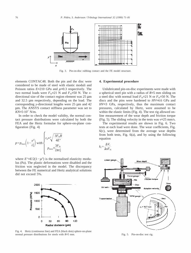
Fig. 3. Pin-on-disc rubbing contact and the FE model structure.

elements CONTAC48. Both the pin and the disc wereconsidered to be made of steel with elastic moduli andPoisson ratiosE=210 GPa andm=0.3 respectively. Thetwo normal loads wereFN=21 N andFN=50 N. Thex-directional size of the contact region element was 25µmand 32.5µm respectively, depending on the load. Thecorrespondingy-directional lengths were 25µm and 42µm. The ANSYS contact stiffness parameter was set toKN=5·107 N/m.

In order to check the model validity, the normal con-tact pressure distributions were calculated by both theFEA and the Hertz formulae for sphere-on-plane con-figuration (Fig. 4)

p5pmaxS12x2

r20D with 5r0=3! 3FNR

4E∗

pmax=3FN

2pr20

whereE∗=E/2(12m2) is the normalised elasticity modu-lus (Pa). The plastic deformations were disabled and thefriction was neglected in the model. The discrepancybetween the FE numerical and Hertz analytical solutionsdid not exceed 5%.

Fig. 4. Hertz (continuous line) and FEA (black dots) sphere-on-planenormal pressure distributions for steels withR=5 mm.

4. Experimental procedure

Unlubricated pin-on-disc experiments were made witha spherical steel pin with a radius ofR=5 mm sliding ona steel disc with normal loadFN=21 N orFN=50 N. Thediscs and the pins were hardened toHV=4.6 GPa andHV=3 GPa, respectively, thus the maximum contactpressures, calculated by Hertz, were assumed to bewithin the elastic limits (Fig. 4). The test rig allowed on-line measurement of the wear depth and friction torque(Fig. 5). The sliding velocity in the tests wasv=25 mm/s.

The experimental results are shown in Fig. 6. Twotests at each load were done. The wear coefficients, Fig.6(c), were determined from the average wear depthsfrom both tests, Fig. 6(a), and by using the followingequation

ki5DVi

DsFN

Fig. 5. Pin-on-disc test rig.


Fig. 6. Pin-on-disc experiment data for steels as a function of sliding distance: (a) pin wear depth; (b) friction coefficient; (c) normal contactpressure and wear coefficient; (d) contact flash temperatures.

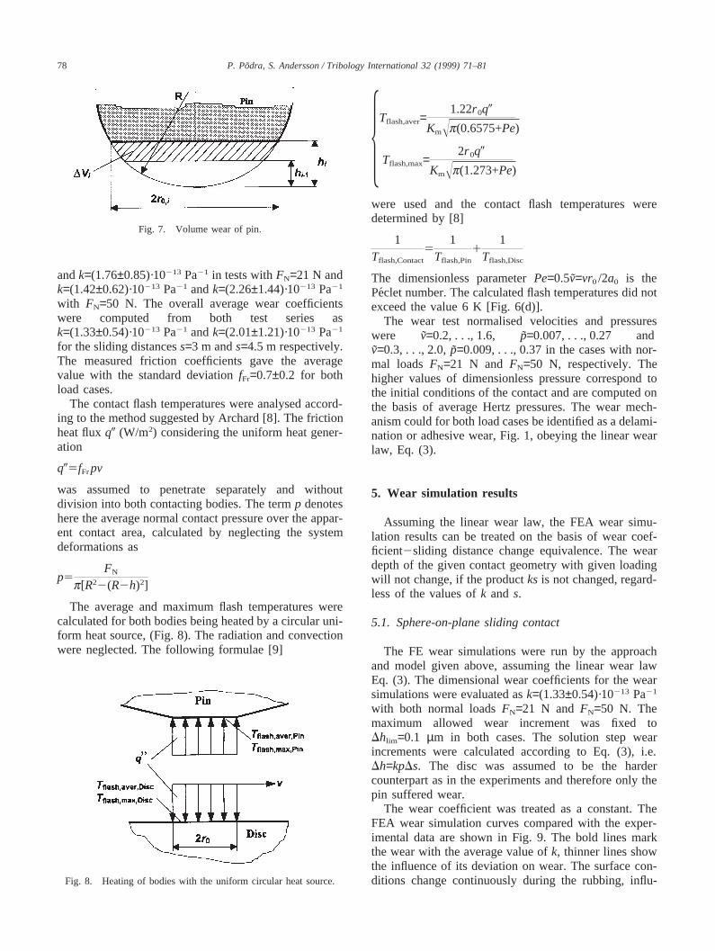
where the volume wear increments were determined bythe formula [7] (Fig. 7)

DVi5p3[h2

i (3R2hi)2h2i−1(3R2hi−1)]

where i$1 is the sampling point number andDs=0.15

m is the sliding distance increment. The discs wereharder than pins and the wear test left no measurableprints on the disc surfaces. The average wear coefficientswere evaluated from experiment data for sliding dis-tancess=3 m ands=4.5 m [Fig. 6(c)]. These values withthe standard deviation werek=(1.25±0.44)·10213 Pa21


Fig. 7. Volume wear of pin.

andk=(1.76±0.85)·10213 Pa21 in tests withFN=21 N andk=(1.42±0.62)·10213 Pa21 andk=(2.26±1.44)·10213 Pa21

with FN=50 N. The overall average wear coefficientswere computed from both test series ask=(1.33±0.54)·10213 Pa21 andk=(2.01±1.21)·10213 Pa21

for the sliding distancess=3 m ands=4.5 m respectively.The measured friction coefficients gave the averagevalue with the standard deviationfFr=0.7±0.2 for bothload cases.

The contact flash temperatures were analysed accord-ing to the method suggested by Archard [8]. The frictionheat fluxq0 (W/m2) considering the uniform heat gener-ation

q05fFrpv

was assumed to penetrate separately and withoutdivision into both contacting bodies. The termp denoteshere the average normal contact pressure over the appar-ent contact area, calculated by neglecting the systemdeformations as

p5FN

p[R22(R2h)2]

The average and maximum flash temperatures werecalculated for both bodies being heated by a circular uni-form heat source, (Fig. 8). The radiation and convectionwere neglected. The following formulae [9]

Fig. 8. Heating of bodies with the uniform circular heat source.

5Tflash,aver=1.22r 0q0

KmÎp(0.6575+Pe)

Tflash,max=2r 0q0

KmÎp(1.273+Pe)

were used and the contact flash temperatures weredetermined by [8]

1Tflash,Contact

51

Tflash,Pin

11

Tflash,Disc

The dimensionless parameterPe=0.5v=vr0/2a0 is thePeclet number. The calculated flash temperatures did notexceed the value 6 K [Fig. 6(d)].

The wear test normalised velocities and pressureswere v=0.2, . . ., 1.6, p=0.007, . . ., 0.27 andv=0.3, . . ., 2.0,p=0.009, . . ., 0.37 in the cases with nor-mal loadsFN=21 N and FN=50 N, respectively. Thehigher values of dimensionless pressure correspond tothe initial conditions of the contact and are computed onthe basis of average Hertz pressures. The wear mech-anism could for both load cases be identified as a delami-nation or adhesive wear, Fig. 1, obeying the linear wearlaw, Eq. (3).

5. Wear simulation results

Assuming the linear wear law, the FEA wear simu-lation results can be treated on the basis of wear coef-ficient2sliding distance change equivalence. The weardepth of the given contact geometry with given loadingwill not change, if the productks is not changed, regard-less of the values ofk and s.

5.1. Sphere-on-plane sliding contact

The FE wear simulations were run by the approachand model given above, assuming the linear wear lawEq. (3). The dimensional wear coefficients for the wearsimulations were evaluated ask=(1.33±0.54)·10213 Pa21

with both normal loadsFN=21 N andFN=50 N. Themaximum allowed wear increment was fixed toDhlim=0.1 µm in both cases. The solution step wearincrements were calculated according to Eq. (3), i.e.Dh=kpDs. The disc was assumed to be the hardercounterpart as in the experiments and therefore only thepin suffered wear.

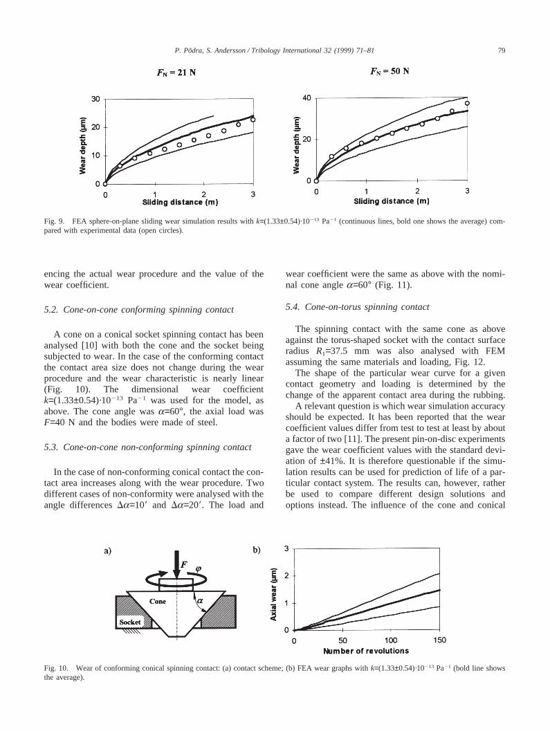
The wear coefficient was treated as a constant. TheFEA wear simulation curves compared with the exper-imental data are shown in Fig. 9. The bold lines markthe wear with the average value ofk, thinner lines showthe influence of its deviation on wear. The surface con-ditions change continuously during the rubbing, influ-


Fig. 9. FEA sphere-on-plane sliding wear simulation results withk=(1.33±0.54)·10213 Pa21 (continuous lines, bold one shows the average) com-pared with experimental data (open circles).

encing the actual wear procedure and the value of thewear coefficient.

5.2. Cone-on-cone conforming spinning contact

A cone on a conical socket spinning contact has beenanalysed [10] with both the cone and the socket beingsubjected to wear. In the case of the conforming contactthe contact area size does not change during the wearprocedure and the wear characteristic is nearly linear(Fig. 10). The dimensional wear coefficientk=(1.33±0.54)·10213 Pa21 was used for the model, asabove. The cone angle wasa=60°, the axial load wasF=40 N and the bodies were made of steel.

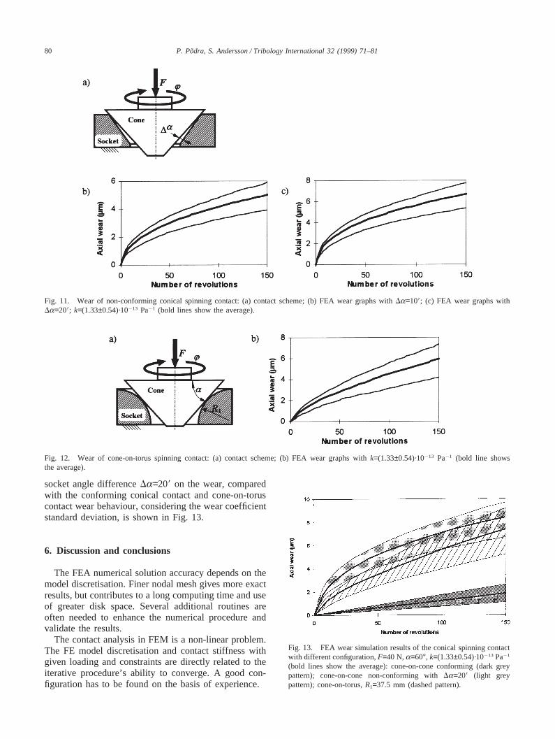
5.3. Cone-on-cone non-conforming spinning contact

In the case of non-conforming conical contact the con-tact area increases along with the wear procedure. Twodifferent cases of non-conformity were analysed with theangle differencesDa=109 and Da=209. The load and

Fig. 10. Wear of conforming conical spinning contact: (a) contact scheme; (b) FEA wear graphs withk=(1.33±0.54)·10213 Pa21 (bold line showsthe average).

wear coefficient were the same as above with the nomi-nal cone anglea=60° (Fig. 11).

5.4. Cone-on-torus spinning contact

The spinning contact with the same cone as aboveagainst the torus-shaped socket with the contact surfaceradius R1=37.5 mm was also analysed with FEMassuming the same materials and loading, Fig. 12.

The shape of the particular wear curve for a givencontact geometry and loading is determined by thechange of the apparent contact area during the rubbing.

A relevant question is which wear simulation accuracyshould be expected. It has been reported that the wearcoefficient values differ from test to test at least by abouta factor of two [11]. The present pin-on-disc experimentsgave the wear coefficient values with the standard devi-ation of ±41%. It is therefore questionable if the simu-lation results can be used for prediction of life of a par-ticular contact system. The results can, however, ratherbe used to compare different design solutions andoptions instead. The influence of the cone and conical


Fig. 11. Wear of non-conforming conical spinning contact: (a) contact scheme; (b) FEA wear graphs withDa=109; (c) FEA wear graphs withDa=209; k=(1.33±0.54)·10213 Pa21 (bold lines show the average).

Fig. 12. Wear of cone-on-torus spinning contact: (a) contact scheme; (b) FEA wear graphs withk=(1.33±0.54)·10213 Pa21 (bold line showsthe average).

socket angle differenceDa=209 on the wear, comparedwith the conforming conical contact and cone-on-toruscontact wear behaviour, considering the wear coefficientstandard deviation, is shown in Fig. 13.

6. Discussion and conclusions

The FEA numerical solution accuracy depends on themodel discretisation. Finer nodal mesh gives more exactresults, but contributes to a long computing time and useof greater disk space. Several additional routines areoften needed to enhance the numerical procedure andvalidate the results.

The contact analysis in FEM is a non-linear problem.The FE model discretisation and contact stiffness withgiven loading and constraints are directly related to theiterative procedure’s ability to converge. A good con-figuration has to be found on the basis of experience.

Fig. 13. FEA wear simulation results of the conical spinning contactwith different configuration,F=40 N,a=60°, k=(1.33±0.54)·10213 Pa21

(bold lines show the average): cone-on-cone conforming (dark greypattern); cone-on-cone non-conforming withDa=209 (light greypattern); cone-on-torus,R1=37.5 mm (dashed pattern).


The integration time step is a critical parameterregarding the reliability of simulation results. Too longsteps cause erratic results and possibly the un-conver-gence of FEA procedure. Too short intervals take toomuch computing time. A simple simulation time stepoptimisation routine was developed, evaluating the inte-gration step duration for every solution step individuallyon the basis of the fixed maximum wear increment.

The wear mechanism must be considered and itschanges must be foreseen during the simulation process.The Lim and Ashby wear map can be used for steels.

Assuming the linear wear law to be valid, the FEAwear simulation results for a given contact geometry anda given load can be treated on the basis of wear coef-ficient2sliding distance change equivalence.

Due to the model simplifications and the real deviationof input data, the FEA wear simulation results should beevaluated on a relative scale to compare different designoptions, rather than to be used to predict the absolutewear life.

References

[1] Meng H-C. Wear modelling: Evaluation and categorisation of wearmodels. Dissertation, University of Michigan, 1994.

[2] Lim SC, Ashby MF. Wear mechanism maps. Acta metall1987;35(1):1–24.

[3] Holm R. Electric contacts. Uppsala: Almqvist and Wiksells Bok-tryckeri AB, 1946.

[4] Archard JF. Wear theory and mechanisms. In: Peterson MB, WinerWO, editors. Wear control handbook. New York: ASME, 1980.

[5] Cook RD. Concepts and applications of finite element analysis.New York: John Wiley and Sons, 1981.

[6] ANSYS User’s manual for revision 5.0, vol. 4, theory. HoustonSwanson Analysis System Inc., 1994.

[7] Spiegel MR. Mathematical handbook of formulas and tables. NewYork: McGraw-Hill Book Company, 1990.

[8] Archard JF. The temperature of rubbing surfaces. Wear1959;2:438–45.

[9] Tian X, Kennedy FE. Maximum and average flash temperatures insliding contacts. Transactions of the ASME, Journal of Tribology1994;116:000–0.

[10] Podra P. FEA wear simulation of a conical spinning contact.Presented at OST-97 Symposium on Machine Design, 22-23 May1997, Tallinn (Estonia).

[11] Rabinowicz E. Wear coefficients—metals. In: Peterson MB,Winer WO, editors. Wear control handbook. New York:ASME, 1980.

Simulation of Sliding Wear

Documents

Transcript of Simulation of Sliding Wear