Power System Dynamic State Estimation With Synchronized Phasor Measurements
Upload
nguyenduongCategory
view
246download
6
Diss. ETH No. 17607
Simulation of Power SystemDynamics using Dynamic
Phasor Models
A dissertation submitted to theSWISS FEDERAL INSTITUTE OF TECHNOLOGY
ZURICH
for the degree ofDoctor of Sciences
presented byTURHAN HILMI DEMIRAY
Dipl. Ing. (TU Wien)born January 14, 1970
citizen of Turkey and USA
accepted on the recommendation ofProf. Dr. Goran Andersson, examiner
Prof. Dr. Aleksandar Stankovic, co-examiner
2008


Contents
1 Introduction 1
1.1 Outline of the Thesis . . . . . . . . . . . . . . . . . . . . 6
1.2 Contributions . . . . . . . . . . . . . . . . . . . . . . . . 7
1.3 List of Publications . . . . . . . . . . . . . . . . . . . . . 7
2 Simulation Framework 9
2.1 Introduction . . . . . . . . . . . . . . . . . . . . . . . . . 9
2.2 Hybrid System Representation . . . . . . . . . . . . . . 11
2.3 Simulation Process . . . . . . . . . . . . . . . . . . . . . 18
2.3.1 Initialization . . . . . . . . . . . . . . . . . . . . 20
2.3.2 Calculation of Continuous Trajectory . . . . . . 21
2.3.3 Event Handling and Consistent Reinitialization . 26
2.4 Automatic Code Generator . . . . . . . . . . . . . . . . 30
2.5 Implementation Issues . . . . . . . . . . . . . . . . . . . 38
2.6 Summary . . . . . . . . . . . . . . . . . . . . . . . . . . 39
3 Modelling of Power Systems 41
3.1 Introduction . . . . . . . . . . . . . . . . . . . . . . . . . 41
3.2 ABC Three-Phase Representation . . . . . . . . . . . . . 43
3.3 Baseband Representation . . . . . . . . . . . . . . . . . 46
3.4 DQ0 Representation . . . . . . . . . . . . . . . . . . . . 49
3.5 Dynamic Phasor Representation . . . . . . . . . . . . . 52
iii

iv Contents
3.6 Summary . . . . . . . . . . . . . . . . . . . . . . . . . . 57
4 Comparative Assessment of Different Modelling Tech-niques 61
4.1 Introduction . . . . . . . . . . . . . . . . . . . . . . . . . 61
4.2 Transmission Line Model . . . . . . . . . . . . . . . . . 63
4.2.1 Dynamic Phasor Model − ABC . . . . . . . . . . 63
4.2.2 Dynamic Phasor Model − DQ0 . . . . . . . . . . 65
4.3 Synchronous Machine . . . . . . . . . . . . . . . . . . . 70
4.3.1 Dynamic Phasor Model − ABC . . . . . . . . . . 71
4.3.2 Dynamic Phasor Model − DQ0 . . . . . . . . . . 78
4.4 Test Cases . . . . . . . . . . . . . . . . . . . . . . . . . . 82
4.4.1 Unbalanced Faults . . . . . . . . . . . . . . . . . 83
4.4.2 Asymmetrical Components . . . . . . . . . . . . 92
4.5 Summary . . . . . . . . . . . . . . . . . . . . . . . . . . 96
5 Dynamic Phasor Model of the DFIG 97
5.1 Introduction . . . . . . . . . . . . . . . . . . . . . . . . . 97
5.2 DFIG Model . . . . . . . . . . . . . . . . . . . . . . . . 99
5.2.1 Drive Train Model . . . . . . . . . . . . . . . . . 99
5.2.2 Induction Machine . . . . . . . . . . . . . . . . . 100
5.2.3 Converter Model . . . . . . . . . . . . . . . . . . 103
5.3 Comparative Assessment of Models . . . . . . . . . . . . 107
5.4 Test Cases . . . . . . . . . . . . . . . . . . . . . . . . . . 108
5.4.1 Balanced Voltage Sag . . . . . . . . . . . . . . . 110
5.4.2 Unbalanced Voltage Sag . . . . . . . . . . . . . . 114
5.5 Summary . . . . . . . . . . . . . . . . . . . . . . . . . . 118
6 Dynamic Phasor Model of the TCSC 119
6.1 Introduction . . . . . . . . . . . . . . . . . . . . . . . . . 119
6.2 Characteristics and Circuit Analysis of TCSC . . . . . . 121
6.3 Steady State Analysis . . . . . . . . . . . . . . . . . . . 124

Contents v
6.4 Fundamental Frequency Dynamic Phasor Model . . . . 130
6.5 Improved Dynamic Phasor Model . . . . . . . . . . . . . 134
6.6 Test Case . . . . . . . . . . . . . . . . . . . . . . . . . . 139
7 Optimization of Numerical Integration Methods for theDynamic Phasors 141
7.1 Introduction . . . . . . . . . . . . . . . . . . . . . . . . . 141
7.2 Linear Multi-step Methods . . . . . . . . . . . . . . . . 143
7.2.1 Error Analysis in Frequency Domain . . . . . . 146
7.2.2 Numerical Stability Analysis . . . . . . . . . . . 147
7.3 Frequency Matched TrapezoidalMethod for Real Signals . . . . . . . . . . . . . . . . . . 148
7.3.1 Error Analysis in Frequency Domain . . . . . . 150
7.3.2 Numerical Stability Analysis . . . . . . . . . . . 152
7.4 Frequency Matched TrapezoidalMethod for Complex Signals . . . . . . . . . . . . . . . . 154
7.4.1 Error Analysis in Frequency Domain . . . . . . 155
7.4.2 Numerical Stability Analysis . . . . . . . . . . . 156
7.5 Test Cases . . . . . . . . . . . . . . . . . . . . . . . . . . 158
7.5.1 Example with Analytic Solution . . . . . . . . . 158
7.5.2 SMIB system . . . . . . . . . . . . . . . . . . . . 159
7.6 Summary . . . . . . . . . . . . . . . . . . . . . . . . . . 163
8 Conclusions and Outlook 165
Bibliography 173
Curriculum vitae 175


Acknowledgements
First of all I would like to express my deepest gratitude to my advisorProf. Dr. Goran Andersson ( Goran Bey ) for giving me the oppor-tunity to write my thesis as a member of his research group. Besideshis excellent guidance and valuable suggestions, I am also grateful forhis positive attitude, encouragement and flexibility as well as for thegranted freedom he gave me to explore different areas of power systems.
A special thanks goes to Prof. Dr. Aleksandar Stankovic for consentingto be the co-examiner and providing a number of valuable commentsand suggestions.
I also wish to thank all my colleagues from the Power System Labora-tory, Antonis, Florian, Michele, Monika, Marija, Marek, the Martins,Matthias, Gaby, Stephan, Gaudenz, Thilo, Christian, Rusejla, Mirjana,Wolfgang and Jost for the pleasant working atmosphere and the lovelysupport they gave me. Our entertaining coffee-breaks and especially the”belly” birthday gift you gave me this year will always remain in mymemory. I am indebted to you all.
Thanks to Andrea Giovanni Beccuti, I had also the opportunity to tastethe great coffee of the Automatic Control Laboratory. Dear Andrea, Ithank you for the close and enjoyable collaboration we had within theframework of HYCON. I am also deeply grateful for your proof-readingof my thesis.
Further, I would like to thank Luigi Busarello and Giatgen Cott fromBCP ( Busarello+Cott+Partner ) for financing this project and thefreedom they granted me during these four years. Especially, I want tothank my Greek sister Tina Orfanogianni Dorn from BCP for the help,support and joy she gave me.
vii

viii Acknowledgements
I am also indebted to my close friends Cem & Pelin Edis, Bulent &Duygu Aydin for their love and support over the years.
Finally, I would like to extend my gratitude to the closest person to me,to my warm-hearted and joyful wife, Handemmm.
Handemmm, I thank you with all my heart for your understanding andthe support you gave me with your pure love.
. . . It is you that this work is dedicated.

Abstract
Computer simulations of electric power systems are an essential partof planning, design and operation in the power industry. Due to theincreased loading of the power systems, the stability has become a con-cern, so that programs for the analysis of the transient behavior of powersystems have become an integral part of system design and control, inorder to maximize the ability of a system to withstand the impact of se-vere disturbances. Generally as large systems are under consideration,simplifying assumptions are often made to facilitate an efficient simula-tion of such large power systems with the so called Transient StabilityPrograms (TSP). In the TSP, the fast electromagnetic transients areneglected and it is assumed that the power transfer takes place at thesystem frequency. The focus in these programs are more on the slowerelectromechanical transients, which have more a system wide effect.However, recent blackouts due to increasingly sensitive operating condi-tions, have created a need for more detailed and comprehensive studies.Such detailed studies including the fast electromagnetic transients aredone with so called Electromagnetic Transient Programs (EMTP). Incontrast to the electromechanical transients, the electromagnetic tran-sients have more a local character so that only a small part of thecomplete power system is usually studied with the EMTP. The simula-tion of the complete power system with the EMTP is computationallyinefficient, since too small simulation step sizes are employed for thecalculation of the fast electromagnetic transients. Hence, the combinedsimulation of the electromagnetic and electromechanical transients is achallenging task.
The aim of this dissertation is to fill the gap between the TSP andEMTP by developing a new simulation tool based on the dynamic pha-sor representation of the power system, which facilitates the combined
ix

x Abstract
simulation of the electromagnetic and electromechanical transients inan accurate, efficient and systematic way. For this purpose, a generaland systematic simulation framework was developed for the simulationof power system transients with the dynamic phasor models of majorpower system components. The accuracy and computational efficiencyof the dynamic phasor model representation were compared with othertraditionally used power system representations. Furthermore, new nu-merical integration algorithms were developed for the accurate and ef-ficient simulation of systems represented by dynamic phasors. The de-veloped prototype of the new simulation tool was implemented in thecommercially used power system analysis program NEPLAN [1].

Kurzfassung
Computersimulationen sind ein essentieller Bestandteil in der Planungund dem Betrieb von elektrischen Energiesystemen. Durch die steigendeAuslastung der elektrischen Netze wird die Stabilitat des Systems zueinem immer wichtigeren Aspekt, so dass Programme zur Analyse vonAusgleichsvorgangen in elektrischen Energiesystemen eine grossere Rol-le bei der Systemplannung und -regelung spielen, um die Widerstands-fahigkeit des Systems im Falle einer grossen Storung zu maximieren.Da normalerweise grosse Systeme betrachtet werden, werden auch oftvereinfachende Annahmen getroffen um eine effiziente Simulation vongrossen elektrischen Netzen mit sogenannten transienten Stabilitatspro-grammen (TSP) zu ermoglichen. In den TSP werden die schnellen elek-tromagnetischen Ausgleichsvorgange vernachlassigt und es wird ange-nommen dass der Leistungstransfer bei der Systemfrequenz stattfindet.Der Schwerpunkt in diesen Programmen liegt mehr auf den langsamerenelektromechanischen Ausgleichsvorgangen. Jedoch haben Systemaus-falle in jungster Vergangenheit das Bedurfnis nach detaillierten und um-fangreicheren Studien erhoht. Fur solch detaillierte Studien werden Pro-gramme zur Simulation der elektromagnetischen Transienten (EMTP)verwendet. Im Gegensatz zu elektromechanischen Ausgleichsvorgangenhaben die elektromagnetischen Vorgange eher lokale Auswirkungen, sodass nur ein kleiner Teil des gesamten Systems mit den EMTP unter-sucht wird. Die Simulation des gesamten Energiesystems mit EMTPist sehr ineffizient, da sehr kleine Schrittweiten fur die Berechnung derschnellen elektromagnetischen Vorgange verwendet werden mussen.
Somit kann man sagen, dass die kombinierte Simulation von elektro-magnetischen und elektromechanischen Ausgleichsvorgangen noch im-mer eine grosse Herausforderung darstellt. Das Ziel dieser Dissertationist die existerende Lucke zwischen den TSP und EMTP zu schliessen,
xi

xii Kurzfassung
indem man basierend auf einer dynamischen Zeigerdarstellung des En-ergiesystems ein neues Simulationsprogram entwickelt, welches die kom-binierte Simulation von elektromagnetischen und elektromechanischenAusgleichsvorgangen in einer genauen, effizienten und systematischenWeise ermoglicht. Fur diesen Zweck wurde mit Modellen von wichtigenNetzkomponenten basierend auf der dynamischen Zeigerdarstellung eineallgemeine und systematische Simulationsumgebung entwickelt. DieGenauigkeit und Effizienz der Modelle wurden mit den herkommlichenModellen verglichen. Daruber hinaus wurden auch numerische Integra-tionsalgorithmen entwickelt, welche fur die genaue und effiziente Simu-lation von Systemen angepasst wurden, die durch dynamische Zeigerdargestellt werden. Der entwickelte Prototyp der Simulationsumge-bung wurde auch in dem kommerziell fur die Planung und Optimierungvon Elektrizitatsnetzen verwendeten Programm NEPLAN [1] imple-mentiert.

Chapter 1
Introduction
The electric power system is today regarded as the most important ofall infrastructure systems built by mankind [2]. Also, other systemssuch as telecommunication, transportation, water supply, etc. are moreor less dependent on a reliable supply of electric power for their properoperation. Consequently, the requirements on the security and relia-bility of the electric power system are very high. Due to the increasedloading of the power systems, the stability has become a concern. Thisis of course accentuated by the recent blackouts in the USA and Europe.In order to achieve the required high level security and reliability, thepower system must be analyzed in detail during planning and operation.The need for simulations in the field of power systems arose already atthe beginning of the 20th century from the impracticability of perform-ing system wide experiments. For this reason, various analytical toolshave been developed to study the dynamic behavior of power systems.Programs for the analysis of the transient behavior of power systemshave become an integral part of system design and control, in order tomaximize the ability of a system to withstand the impact of a severedisturbance.
Time-domain simulation programs are an integral part of the powersystem analysis tools. With the time-domain simulation programs thedynamic response of a power system to disturbances or to changes in thesystem state can be computed by using the appropriate mathematicalmodels and numerical algorithms.
The dynamic phenomena in power systems can be classified into differ-
1

2 Chapter 1. Introduction
10−7 10−5 10−3 10−1 101 103 105
Time (sec)
Electromechanical TransientsElectromagnetic Transients
Lightning
Switching
Stator TransientsSubsynchronous Resonance
Transient Stability
Long term Dynamics
Figure 1.1: Time frame of power system transients
ent time ranges [3]. As depicted in Figure 1.1, the time range of thepower system transients varies from microseconds (Lightning) to hoursand days (Long term dynamics). The overall time range of power sys-tem transients is generally classified into fast electromagnetic transientsand slow electromechanical transients. Thus, the complete power sys-tem can be seen as a coupled electromechanical and electromagneticsystem with a wide range of time constants. There are fast electro-magnetic transients due to the interaction between the magnetic fieldsof inductances and electrical fields of capacitances. Besides, there arealso slower electromechanical transients due to the interaction betweenthe mechanical energy stored in the rotating machines. Generally, dif-ferent time-domain simulation tools are used for studying the differentdynamic phenomena in power systems.
Electromagnetic transient phenomena are usually triggered by changesin the network configuration. Such changes may be due to the closing oropening action of circuit breakers or power electronic equipment, or byequipment failure or faults. These phenomena are more local in char-acter. This fast electromagnetic transients are typically studied withthe Electromagnetic Transients Programs (EMTP) [4]. As fast dynam-

3
ics are of concern, the simulation step size is of the order of tens ofmicroseconds but can even be smaller depending on the type of electro-magnetic phenomenon being studied. Due to the long time constantsassociated with the dynamics of power plants, such as generators andturbines, simplified models of such devices are often sufficient for thetime frame of typical electromagnetic transients studies.
Electromechanical transients are slower transients that are due to theinteraction between the mechanical energy stored in the rotating ma-chines and the electrical energy stored in the electrical network. Amismatch between the mechanical energy and the electrical energy in-volves the oscillation of machine rotors because of an unbalance betweenturbine and generator torques. The analysis of this class of transientsis known as transient stability simulation. Such studies are done withthe so called transient stability programs (TSP) (e.g. SIMPOW [5] ,EUROSTAG [6]). An important assumption for this type of analysisis that the exchange of energy between generators and other dynamicequipment takes place with the electric network remaining at powerfrequency (system frequency). With this assumption, electromagnetictransients cannot be properly represented and are neglected during thesimulation process. This is achieved by using the steady-state phasorrepresentation of the electrical network quantities at the system fre-quency. This approach is referred to as the quasi-steady state approachin the literature. The omission of the fast electromagnetic transientsallows the transient stability simulation programs the use of larger stepsizes. These transient stability programs usually include models of dif-ferent power system components that are appropriate for phenomenathat have characteristic time constants that are about a hundred mil-liseconds or larger. With these simulation programs, very large powersystems could be studied, e.g. interconnected system of Western Europe- UCTE. The phenomena of concern in these studies are quite often sys-tem wide, and the complete system needs in many cases to be includedfor meaningful analysis.
For a long period of time, the electromagnetic transients programs andtransient stability programs have not been unified in a common simu-lation program. Reasons for the separate use of these programs are:
• The objectives of electromagnetic transients analysis and of tran-sient stability analysis are different. In the electromagnetic tran-sients analysis one investigates fast transient phenomena that usu-

4 Chapter 1. Introduction
ally decay rapidly and have no impact on the slower system dy-namics. In the transient stability analysis the aim is to study theimpact of a severe disturbance on the whole power system.
• It is technically possible to perform a transient stability analysisalso in an EMTP. But the required simulation time in an EMTPwould increase drastically due to the following reasons:
– the longer time span of the transient stability simulationscompared with the electromagnetic transients analysis.
– the use of much smaller integration step sizes in an EMTPcompared with the traditional transient stability programs.
– the size of the power system to be simulated in transient sta-bility simulations is much larger than that is typically usedin electromagnetic transients analysis. Because of the lo-cal character of electromagnetic transients due to the higherdamping, the size of the power system is much smaller com-pared with the transient stability analysis.
• Both program types generally use different system representationsfor the modelling of the components and also different integrationmethods to facilitate an efficient simulation of the transient phe-nomena under consideration.
Because of the above mentioned problems, the combined simulation ofthe electromagnetic and electromechanical transients has always been achallenging task.
There are different approaches to overcome this problem. In the sim-ulation program SIMPOW [7], the full network equations and machineequations are described in the DQ0 reference frame which is rotatingwith the system frequency. This representation of the system equa-tions in the DQ0 reference frame increases the simulation efficiency sig-nificantly under balanced conditions, since the variations in the DQ0transformed quantities are much slower than the instantaneous ABCquantities. SIMPOW has two simulation modes, one for electromag-netic and another for electromechanical transients. There is also thepossibility to switch between these modes during the simulation. Suchchanges in the simulation mode become clearly visible with jumps in thestate variables whenever the program switches from the EMTP-modeto the transient stability mode. These artificial jumps may cause e.g.

5
a trip of a protective relay, thereby altering the system configurationincorrectly.
Other approaches combine the electromagnetic and electromechanicalsimulations by representing the full network and machine differentialequations without making the quasi-steady state approximation andsimulate the complete system in the EMTP mode. This is achieved byusing an efficient solution algorithm that is accurate and numericallystable for a wide range of frequencies. Efforts in this direction havebeen reported in [8, 9, 10]. Some important issues related to the workin [9, 10] will be discussed in Chapter 3.
Recent developments, particularly the introduction of more power elec-tronics based equipment e.g. HVDC and FACTS components, also in-crease the need for the detailed time-domain simulation of such devices,since the transient stability programs based on fundamental frequencyphasor modelling techniques cannot directly represent the faster tran-sients characterizing the HVDC and FACTS systems. One approachto overcome this problem, is to model and simulate some parts of thesystem with a detailed full time domain representation and the rest ofthe system in the quasi-steady state representation and interface thedifferent modelling approaches appropriately. In [11, 12], this approachwas used to simulate the HVDC and FACTS transient/dynamic behav-ior in a power system based on an interactive execution of a TSP andan EMTP.
On the other hand efforts have also been made to decrease the lack ofaccuracy of the fundamental frequency phasor models of the FACTS.For this purpose, the concept of generalized averaging method, also re-ferred to as dynamic phasors approach, was proposed in [13] to modelpower electronics based equipment. The main idea behind this methodis to represent the periodical or nearly periodical system quantities notby their instantaneous values but by their time varying Fourier coeffi-cients (dynamic phasors). The variations of the time varying Fouriercoefficients are much slower than the original instantaneous values. Theapplication of this method was then extended to model FACTS devices[14, 15, 16] to increase the accuracy of the fundamental frequency phasormodels. The same approach has also been applied to model electricalmachines under unbalanced conditions [17, 18, 19].
As mentioned previously, the need for a simulation tool which is ableto simulate the electromagnetic and electromechanical transients in an

6 Chapter 1. Introduction
efficient and accurate way is the main incentive of this research project.Hence, the objective of this thesis is to develop a systematic conceptfor the combined simulation of electromagnetic and electromechanicaltransient phenomena. To achieve this goal, a new simulation tool willbe developed which is based on the dynamic phasors representation ofthe power system. A general and systematic simulation framework willbe developed including the appropriate numerical methods to computethe system response represented by dynamic phasors efficiently. Thedynamic phasor models of the major power system components will bedeveloped and implemented in the new simulation tool. The new systemrepresentation with dynamic phasors will be compared systematicallywith other commonly used system representations in the power systemanalysis in terms of accuracy and computational efficiency.
1.1 Outline of the Thesis
Following the introduction, in Chapter 2, a general and systematic sim-ulation framework will be developed for the simulation of power systemtransients, which will then be also used throughout the thesis.
Chapter 3 gives an overview of the different system representations usedin the area of power systems analysis. For the theoretical assessment ofthe simulation performance of these modelling techniques, the differentsystem representations will be examined in the frequency domain.
In Chapter 4, the dynamic phasor models of major power system com-ponents will be derived and their simulation performance will be com-pared to other commonly used model/system representations in termsof accuracy and computational efficiency.
In Chapter 5 the dynamic phasor model of the doubly-fed inductiongenerator (DFIG) will be derived. The derived model will then be usedto study the dynamic response of the DFIG to balanced and unbalancedvoltage sags.
Chapter 6, the dynamic phasor model of Thyristor-Controlled SeriesCapacitor is derived based on previous work done by Mattavelli et al.[14] and the accuracy and simulation efficiency of the model is comparedwith the detailed time domain model and other existing fundamentalfrequency models.

1.2. Contributions 7
The focus in Chapter 7 is on the derivation of methods suitable forthe numerical integration of systems represented by dynamic phasors.This is achieved investigating the numerical integration techniques inthe frequency domain.
Finally Chapter 8 concludes the thesis by summarizing and discussingthe most important achievements and suggesting possible future work.
1.2 Contributions
The main contributions of this PhD studies research work can be sum-marized as follows:
• A new simulation tool has been developed for the combined simu-lation of electromagnetic and electromechanical transients, whichis based on the dynamic phasor representation of the power sys-tem.
• Dynamic phasor models of major power system components, in-cluding the DFIG, have been derived and implemented.
• A systematic comparison of the dynamic phasor approach hasbeen made with the existing power system representations regard-ing accuracy and computational efficiency.
• A new numerical integration method based on the trapezoidalmethod has been developed, which is optimized for the numericalintegration of systems represented by dynamic phasors.
1.3 List of Publications
Publications related to the Topic of the Thesis
[1 ] T. Demiray and G. Andersson, ”Simulation of Power SystemsDynamics using Dynamic Phasor Models” Presented at the Xth
SEPOPE, Florianopolis, Brasil, May-2006
[2 ] T. Demiray and G. Andersson, ”Comparison of the Efficiency ofDynamic Phasor Models Derived from ABC and DQ0 Reference

8 Chapter 1. Introduction
Frame in Power System Dynamic Simulations” Presented at the7th IEE International Conference on Advances in Powers SystemControl, Operation and Management, 30 October - 2 November,Hong Kong, 2006.
[3 ] T. Demiray, F. Milano and G. Andersson, ”Dynamic PhasorModeling of the Doubly-fed Induction Generator under UnbalancedConditions” Presented at the PowerTech Conference, Lausanne,Switzerland, 2007.
[4 ] T. Demiray and G. Andersson, ”Using Frequency-Matched Nu-merical Integration Methods for the Simulation of Dynamic Pha-sor Models in Power Systems” Submitted to the Power SystemComputation Conference PSCC, Glasgow, Scotland, 2008.
Other Publications in the Project
[5 ] A.G. Beccuti, T. Demiray, M. Zima, G. Andersson and M.Morari, ”Comparative Assessment of Prediction Models in Volt-age Control” Presented at the PowerTech Conference, Lausanne,Switzerland, 2007.
[6 ] R.R. Negenborn, A.G. Beccuti, T. Demiray,S.Leirens, G. Damm,B. De Schutter and M. Morari, ”Supervisory Hybrid Model Predic-tive Control for Voltage Stability of Power Networks” Presentedby at the American Control Conference, New York City, USA,July 11-13, 2007.

Chapter 2
Simulation Framework
In this chapter, a general and systematic simulation framework is devel-oped for the simulation of power system transients. The chapter startswith an introduction to the Differential Switched Algebraic State-Resetrepresentation, which is used as a systematic and general mathemat-ical representation for the hybrid dynamic behavior of power systems.Based on this representation a modular and flexible simulation environ-ment will be developed. Important procedures of the simulation processand some implemented tools facilitating the model development for themodeler will be covered in more detail. The chapter ends with a powersystem case study showing the capabilities of the implemented simulationenvironment.
2.1 Introduction
The dynamic behavior of physical systems are often studied with appro-priate simulation programs. Simulation programs consist of appropriatemathematical models describing the relationship between the quantitiesthat can be observed in the system as mathematical relations and nu-merical methods that are used for the numerical calculation of the com-plex system behavior where a closed form analytic solution can not bespecified. In the power system transient analysis, component models canbe described by Ordinary Differential Equations (ODEs), Differential-Algebraic Equations (DAEs) or Partial Differential Equations (PDEs)
9

10 Chapter 2. Simulation Framework
depending on the nature of the study. For example, if the purpose ofthe study is more local and the interest is on the distribution of elec-tromagnetic fields along a transmission line in a power system, then adistributed parameter representation with Partial Differential Equationswill be used as a mathematical representation for the transmission linemodel. If the purpose of the study is the interconnection of the trans-mission line with other components in the system, where interactionbetween electromagnetic fields of different components is of concern,a lumped parameter representation (R,L,C) with Ordinary DifferentialEquations would be sufficient as a mathematical representation. If ourconcern is on slower and more system wide electromechanical transients,even the electromagnetic transients of the transmission line can be ne-glected and its behavior can be described by simple algebraic equations.
Furthermore, the choice of an adequate mathematical model represen-tation also depends on the characteristics of the system under investi-gation and thus of the components which build up the system. For ex-ample, electrical power system is composed by several components thatform a large-scaled system. There are large generation units such ashydro plants, thermal plants having slow continuous dynamic behaviorwith large time constants in order of a few seconds. But there are alsocontrollers such as Automatic Voltage Regulators (AVR) showing fastcontinuous dynamics with time constants in order of fifty milliseconds.Components such as tap changing transformers and protection devicesexhibit also discrete dynamics due to discrete behavior e.g. transformertap positions and protection relay logics. As the whole power systemis interconnected, there is a permanent interaction between these con-tinuous and discrete dynamics. The mathematical representation ofthe models should capture both continuous and discrete nature of thecomponents.
Another important criterion in the selection of the mathematical repre-sentation of a system is the linearity. If all the operators in a mathemat-ical model present linearity, the resulting mathematical model is definedas linear otherwise nonlinear. There are approaches where the nonlinearsystem behavior is approximated by piecewise linear system behavior.In such cases computationally efficient methods and algorithms for lin-ear systems are applied to compute the system behavior. The efficiencyof these piecewise linear approximations depend on the degree of thesystem nonlinearities. Also in power systems there are many sources ofnonlinearities. For example some nonlinearities are inherent to compo-

2.2. Hybrid System Representation 11
nents, like magnetic saturation of iron core or other nonlinearities arein the mathematical relation between the quantities of the system e.g.the relation between active power, voltage magnitude and voltage angleP = V1V2
Xsin (θ1 − θ2).
Accordingly power systems can be described as a large-scale, non-linear system with fast/slow continuous and discrete dynamics.This permanent interaction between continuous and discrete dynamicsmakes power systems an important class of hybrid systems. The usedmathematical representation should be capable of capturing all thesecharacteristics of the power system in a mathematical formulation. Ourfocus in the following section will be on the mathematical system rep-resentation proposed in [20] and [21], which captures all the importantaspects of power systems. This representation will be then used assystem/model representation throughout the thesis.
2.2 Hybrid System Representation
An adequate mathematical representation for power systems shouldcapture the nonlinear continuous and discrete dynamics. Such systems,where the system behavior is governed by both discrete and continuousstates, are called Hybrid systems. In hybrid systems, there is such astrong coupling between these discrete and continuous behavior of thesystem, so that they must be analyzed simultaneously.
Hybrid systems are characterized by:
• continuous and discrete states
• continuous dynamics
• discrete events
• mappings that define the evolution of discrete states at events
Conceptually, a hybrid system can be thought as a directed graph asillustrated in Figure 2.1, where the nodes describe the continuous dy-namic system behavior at a given mode and the edges show the condi-tions and directions of the transition from one system mode to another.If one transition condition is fulfilled, the system jumps from one mode

12 Chapter 2. Simulation Framework
System at Mode 1
System at Mode 2
System at Mode 3System at Mode 4
y1 > 0
y2 < 0 ∨ y4 < 0
y3 == 0
y4 > 0
y5 < 0
Figure 2.1: Directed graph view of a hybrid system
to an other and remains there, till another transition condition is ful-filled, which takes the system to one other mode. The jumping reflectsthe influence of the discrete event behavior and is dependent both ontrigger condition and the discrete state evolution mapping.
In power systems, the continuous system behavior at different modes canbe described by Differential-Algebraic Equations (DAEs). The discreteevents or switching actions inherent in power systems force the systemto jump to another system mode as illustrated in Figure 2.1, where thecontinuous behavior of the system is described by another set of DAEs.This jump to new set of DAEs can be caused due to a change in adiscrete state variable e.g. tap position of a tap changing transformer.
As proposed in [20] and [21], such a hybrid system behavior can bemodeled by a set of Differential, Switched Algebraic and State Resetequations (DSAR) as given in equations (2.1) - (2.5).
x = f(x, y, z, λ) (2.1)
z = 0 (2.2)
0 = g(0)(x, y, z) (2.3)
0 =
{
g(i−)(x, y, z, λ) ys,i < 0
g(i+)(x, y, z, λ) ys,i > 0i = 1,..., s (2.4)
z+ = hj(x−, y−, z−, λ) yr,j = 0 j = 1,..., r (2.5)

2.2. Hybrid System Representation 13
It can easily be seen, that (2.1) describes the differential equations, (2.3)and (2.4) the so called switched algebraic equations and (2.5) the statereset equations, where
• x are continuous dynamic states
• z are discrete states
• y are algebraic states
• λ are parameters
of the system. The superscript − stands for pre-event values and + forpost event values. At the beginning, the system behavior is describedby the DAE given in (2.1) and (2.3). A transition to another set of DAEtakes place if the corresponding transition condition is fulfilled. Suchtransition conditions are checked by means of so called event variablesys and yr. The ys determine the switching events and yr state resetevents. An event is triggered by an element of ys changing sign and/oran element of yr passing through zero. By switching events, which arecaused by ys sign changes, the functional description of the system ischanged from g(i−)(x, y) to g(i+)(x, y). If we look at the formulation(2.2) and (2.5), we see that the discrete states z are constant betweenevents (z = 0) and at state reset events caused by yr the values ofthe discrete states change according to the state reset functions hj . Atstate reset events, the values of dynamic states x are continuous, whichis most often the case in physical systems. The equations (2.1)-(2.5)capture all the important aspects of a hybrid system.
Large system models are most effectively built using a modular repre-sentation. In a modular representation, the components of the systemare grouped together as subsystems, and then the subsystems are com-bined to build up the complete system. A modular representation canbe designed in a causal or non-causal manner.
In causal modelling, the model behavior is described by a rigid in-put/output relation (e.g. y = f(u)). Causal modelling is like a methodcomputing output values (y) by operating on input values (u). Somevariables of the model are defined as inputs and some as outputs. Theoutput (y) can be calculated if the input (u) is defined. Building systemsby connecting such causal models means using the output of one model

14 Chapter 2. Simulation Framework
as an input to another model. For example, the MATLAB based simu-lation program SIMULINK [22] uses the causal modelling approach.
The major difference between non-causal modelling and causal mod-elling is that there is no distinction between input and output variablesin the non-causal representation. In non-causal modelling, variables areinvolved in equations that must be satisfied, to reflect the componentsbehavior. Systems in non-causal modelling are built by simply con-necting the interface variables of the models. The behavior of such aninterconnected system is defined in terms of the signals that satisfy boththe modules behaviors and the interconnection constraints induced bythe interconnection architecture. One of the advantages of non-causalmodelling is that it allows the modeler to use directly the model equa-tions and variables, meaning that he does not need to specify directlyinput and output signals and their relation in an explicit form. Non-causal modelling also supports component hierarchies, allows the reuseof modelling knowledge in an object-oriented manner, which is the stateof the art in today’s software development. For example, MODELICA[23] uses the non-causal modelling approach.
The DSAR structure allows also a modular and non-causal model repre-sentation, where the component model behavior is described by simplywriting the equations and variables of the component model in the pro-posed form given in (2.1)-(2.5).
With minor modifications and extensions the following structure can beused for a modular component model representation.
xk = fk(xk,yk, zk,λk) (2.6)
zk = 0 (2.7)
0 = g(0)k (xk,yk, zk) (2.8)
0 =
{
g(i−)k (xk,yk, zk,λk) yi
k,s < 0
g(i+)k (xk,yk, zk,λk) yi
k,s > 0i = 1,..., s (2.9)
z+k = h
jk(x
−k ,y
−k , z
−k ,λk) y
jk,r = 0 j = 1,..., r (2.10)
with the following definitions
• xk is a vector of continuous dynamic states of the kth model

2.2. Hybrid System Representation 15
• zk is a vector of discrete states of the kth model
• yk,i are internal algebraic states of the kth model
• yk,s are algebraic states determining the switching events of the
kth model
• yk,r are algebraic states determining the state reset events of the
kth model
• yk,ext are external algebraic states of the kth model, which serveas interface variables to other models
• yk is a vector of all algebraic states of the kth model, which isunion of yk,i, yk,s, yk,r and yk,ext.yk = yk,i ∪ yk,s ∪ yk,r ∪ yk,ext
• λk is a vector of parameters of the kth model
• fk is a vector of differential equations of the kth model
• gk is a vector of algebraic equations of the kth model
• hk is a vector of state reset equations of the kth model
Thus the model is described by defining the variables (xk,yk, zk,λk)of the model and the equations (fk, gk,hk) of the model which mustbe satisfied. But, if it comes to build a system or subsystem consistingof such models, the interface variables of the models must be linkedtogether. Hence, the behavior of such an interconnected system is de-termined in terms of the signals or variables that satisfy both the modelbehaviors and the interconnection constraints induced by the link equa-tions. To illustrate the interconnection or linking concept, we considerthe system depicted in Figure 2.2 consisting of three models, each ofthem having 2 variables and 1 algebraic equation relating these 2 vari-ables together. If we look only at the model equations, we have anunder-determined system with 6 variables (y1,1, y1,2, y2,1, y2,2, y3,1, y3,2)and 3 equations (g1, g2, g3).
g1(y1,1, y1,2) = 0
g2(y2,1, y2,2) = 0
g3(y3,1, y3,2) = 0

16 Chapter 2. Simulation Framework
x = f(x, y, z)z = 0
0 = g(0)(x, y, z)
0 =
{g(i−)(x, y, z)
g(i+)(x, y, z)
ys,i > 0ys,i < 0
}
z+ = hj(x−, y−, z−) yr,j=0
DSAR structure
Model1
Model2
Model2
g1(y1,1, y1,2) = 0
g2(y2,1, y2,2) = 0
g2(y2,1, y2,2) = 0y1,1 y1,2 y2,1y2,2
y3,1 y3,2
y1,1 = y3,1
y1,2 = y2,1
y2,2 = y3,2
Figure 2.2: Illustrative Example of a system consisting of models rep-resented in DSAR structure
The 3 missing equations, to determine the system completely, are givenby the link equations
y1,1 − y3,1 = 0
y1,2 − y2,1 = 0
y2,2 − y3,2 = 0
which are shown as dotted connections in Figure 2.2. Now we have asystem with 6 unknowns and 6 equations, which is a necessary conditionfor the solvability of the system. The link equations are simple linearalgebraic equations. In a system consisting of m models, they can beformulated as
c(y1,ext,y2,ext, ......,ym,ext) = 0
The structure of such a system can be illustrated in a two dimensionalarray as shown in Figure 2.3. The horizontal axis contains all the con-tinuous dynamic states x and algebraic states y. States belonging to the

2.2. Hybrid System Representation 17
x y
f
g
c(y1..y4)
x1 x2 x3 x4 y1 y2 y3 y4
f1(x1, y1)
f2(x2, y2)
f3(x3, y3)
f4(x4, y4)
g1(x1, y1)
g2(x2, y2)
g3(x3, y3)
g4(x4, y4)
c
Figure 2.3: Illustration of the overall System Function Structure
same model are also grouped together. In the vertical axis, the modelequations are listed. First the differential equations f , then the alge-braic equations g followed by the connection equations c are listed. Itcan easily be seen that each model equation is only described by its ownstates e.g. g1(x1, y1). This can be seen as a block diagonal structure inthe two dimensional representation. The overall dependence is finalizedby the connection matrix, which here in this illustrative representationcovers the entire range of y variables. Normally only interface variablesyk,ext of the models are involved in the link equations. This represen-tation, shows a sparse structure. The shaded areas in the Figure showthe maximum possible dependence of the model functions on the modelvariables meaning, if all f and g equations of one model will depend onall dynamic states and algebraic states (x, y), which is normally not thecase. Normally, these equations and also the connection equations aresparse, which is also reflected in the overall structure.
The sparsity of the overall system representation in Figure 2.3 becomes
18 Chapter 2. Simulation Framework
also noticeable in the system matrices used during the numerical calcu-lation of the system trajectory.
In this section, the focus was on the employed hybrid system repre-sentation DSAR, which captures all the important aspects of hybridsystems. The DSAR is general, systematic and allows a modular andobject oriented system representation.
2.3 Simulation Process
In the previous sections, our focus was on a systematic and general sys-tem and model representation. This section deals with the implementa-tion issues of the simulator based on the DSAR model representation.
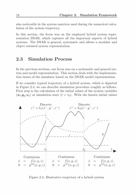
If we consider typical trajectory of a hybrid system, which is depictedin Figure 2.4, we can describe simulation procedure roughly as follows.First step is the calculation of the initial values of the system variables(x0,y0,z0) at simulation start (t = t0). With the known initial values
x = f(x, y, z)0 = g(0)(x, y, z)
x = f(x, y, z)
0 = g(1)(x, y, z)
x = f(x, y, z)0 = g(2)(x, y, z)
z+ = h1(x−, y−, z−) z+ = h2(x
−, y−, z−)DiscreteDiscrete
ContinuousContinuousContinuous
tt1 t2
x
z y
Figure 2.4: Illustrative trajectory of a hybrid system

2.3. Simulation Process 19
of the variables, the continuous system trajectory can be calculated byusing appropriate numerical integration techniques. This continuoussystem trajectory calculation lasts till an event forces the system toswitch to another mode, where the system is described by another setof equations. This so called event handling is a crucial part of hybridsystem simulation. After the correct event handling, the values of thesystem variables in the new mode are calculated at t = t1 and thesevalues are the initial conditions for the new continuous section. Theseprocedures are repeated until the simulation end time is reached. Figure
yes
yes
no
no
Initialization
x0, y0, z0, t0
t < tend End
Calculation of
Continuous trajectory
Event detected
Event handling and
Reinitialization
x+e , y+
e , z+e , te
Figure 2.5: Simplified flow chart of the overall simulation
2.5 shows the simplified flow chart of the overall simulation process,where x+
e , y+e , z
+e denote the calculated post-event values of the system
variables and te the calculated event time.
In the following, the three major tasks of the simulation process will bediscussed, namely:

20 Chapter 2. Simulation Framework
• Initialization
• Calculation of continuous system trajectory
• Event handling and Reinitialization
2.3.1 Initialization
Initialization procedure computes or specifies the initial values of thecontinuous dynamic states x0 and algebraic states y0, which are requiredto start the numerical integration at the very first time step. In theimplemented simulation framework, there are 2 different initializationmodes available:
• Initialization with predefined dynamic states
• Initialization at steady-state
In the Initialization with predefined dynamic states the user supplies theexact initial values of the dynamic states x = x0 and the initial guess ofthe algebraic values y = y0 at t = t0. In this case, as the dynamic statesare predefined, the initial values of algebraic states y0 must satisfy thealgebraic equations g and the connection equations c at t = t0 given as:
0 = g(x0, y)
0 = c(y)
The solution of the this nonlinear equation in y with an iterative Newtonmethod will provide us with the initial values of the algebraic variablesy0. In this case, the system is generally not in steady-state (x 6= 0).
In the initialization mode at steady-state, all derivatives of dynamicstates are set to zero. This means a constraint on x at t = t0 is putnamely x|t=t0 = 0. Now initial values x0 are also unknown and thesolution of the equation
x|t=t0 = 0 = f(x, y)
0 = g(x, y)
0 = c(y)

2.3. Simulation Process 21
after x and y gives the initial values for dynamic states x = x0 andalgebraic states y = y0.
The numerical solution of these nonlinear algebraic equations are per-formed with the Newton-Raphson Method and will be treated in thenext section, as such nonlinear equations and their numerical solutionis also an important task during the calculation of the continuous systemtrajectory.
2.3.2 Calculation of Continuous Trajectory
Now, we will deal with the numerical computation of the continuoustrajectory between events described by a system DAEs.
A system of nonlinear ordinary differential equations such as x = f(x, t)cannot be solved analytically but must be solved numerically [24]. Thebasic concept of a numerical solution algorithm is to approximate thetrue solution of x(t) at a set of time points t0, t1, ....tn by the calculatedvalues x0, x1, ....xn. This approximation is done by advancing the solu-tion from tn to tn+1 = tn +∆tn+1 with integration step size ∆tn+1 andcalculating xn+1 as a function of ∆tn+1, previously calculated statesxn, ..., xn−m and derivatives x(tn), ..., x(tn−m). A generalized formula-tion for such a numerical integration method is:
xn+1 = Ψ (∆tn+1, [xn, xn−1, ..], [f(xn+1), f(xn), ..]) (2.11)
In this formulation, the function Ψ is called Discretization Function ofthe numerical integration method.
For the numerical solution of systems described by DAEs, Gear [25] pro-posed the simultaneous solution approach, where the differential and al-gebraic equations of the system are solved together. The used numericalintegration method discretizes the differential equation at t = tn+1 withthe discretization function Ψ as shown in equation (2.11) and convertsit into a set of nonlinear algebraic equations, which must be satisfied att = tn+1. At t = tn+1 the system variables must satisfy not only thediscretized differential equations but also the algebraic equations g andthe algebraic connection equations c. At t = tn+1, the set of equations,which have to be solved, is given as
xn+1 = Ψ(∆tn+1, xn, ..., xn−m, f(xn+1, yn+1), f(xn, yn)...)
0 = g(xn+1, yn+1)
0 = c(yn+1)

22 Chapter 2. Simulation Framework
After bringing xn+1 to the right side of the equation, the DiscretizedSystem Function at t = tn+1 can be formulated as:
0 = Ψ(∆tn+1, xn, ..., xn−m, f(xn+1, yn+1), f(xn, yn)...) − xn+1
0 = g(xn+1, yn+1)
0 = c(yn+1)
With χ = [xn+1yn+1]T, a vector consisting of all unknown variables
xn+1, yn+1, the expression becomes
F (χ) =
Ψ(∆tn+1, f(xn+1, yn+1), f(xn, yn), ......) − xn+1
g(xn+1, yn+1)c(yn+1)
= 0 (2.12)
In this formulation, the history terms xn, ..., xnm, yn..., yn−m and inte-
gration step size ∆tn+1 are known, xn+1 and yn+1 are unknown. Thecomplete set of discretized system equations F (χ) at t = tn+1 is non-linear and can be solved with Newton-Raphson algorithm. Newton-Raphson method is the standard method used for the numerical solutionof nonlinear algebraic equations and is explained in many text books inmore detail (e.g. [24]). The main idea of the method is illustrated inFigure 2.6 for a one dimensional case f(x) = 0. Starting with an initialguess x0 which is reasonably close to the true solution, the function isapproximated by its tangent line and the intercept of this tangent lineis calculated x1. This intercept is typically a better approximation tothe function’s root than the original guess, and the method is iteratedtill |f(xi)| ≤ ε. At each iteration xi+1 is calculated by
xi+1 = xi −f(xi)
f ′(xi)
where i denotes the iteration counter. In the multidimensional case ofthe discretized system function, this is formulated as
χi+1 = χi − F−1χ (χi)F (χi) (2.13)
If the convergence is reached, we have our solutions for xn+1 and yn+1,at t = tn+1. As shown in (2.13), for solving this set of nonlinear equa-tions F (χ) = 0, we need to evaluate F (χ) (2.12) and the Jacobian Fχ(2.14) at each iteration.
Fχ(χ) =
(Ψf fx − I) (Ψf fy)gx gy0 cy
(2.14)

2.3. Simulation Process 23
f(x)
f(x)
xx0x1x2
Figure 2.6: One iteration of Newton-Raphson method in one dimen-sional case
Independent of the used numerical integration method, a large set ofnon-linear algebraic equations (2.12) has to be solved iteratively at everysimulation time step.
F (χ) (2.12) is dependent on
• the used numerical integration method Ψ.
• the model equations f and g.
• the topology equations c.
In Fχ(χ) (2.14) we need the partial derivatives of
• the used numerical integration method Ψf .
• the models equations fx, fy, gx and gy.
• the topology equations cy
During the simulation process, functions of the numerical integrationmethod (Ψ and Ψf ), the model equations (f , g, fx, fy, gx and gy) andthe topology equations (c, cy) must be evaluated. With such an ab-straction, the simulation framework can be structured in a hierarchicaland object-oriented manner. Figure 2.7 shows the interface between thesimulation kernel and simulated system model. It shows the details of

24 Chapter 2. Simulation Framework
f ,fx,fy,g,gx,gy,h and ys,yr
f ,fx,fy,g,gx,gy,h and ys,yr
f ,fx,fy,g,gx,gy,h and ys,yr
Simulation Kernelc(y),cy
Ψ,Ψf ,Ψ∆t
t,x,y t,x,y
t,x,y
Model1 Model2
Model3
DSAR DSAR
DSAR
y1,1 y1,2 y2,1 y2,2
y3,1 y3,2
Figure 2.7: Model - Simulation Kernel interface
the information exchange between the system model and the simulationkernel.
The choice of the most suitable numerical integration method dependshighly on the characteristics of the simulated system. A combined sim-ulation of transient and long term phenomena in power systems requiresthe solution of a large nonlinear stiff set of differential-algebraic equa-tions. Stiff systems are systems exhibiting a wide-range of time varyingdynamics from very fast to very slow dynamics. Besides accuracy andefficiency, the numerical stability of the used integration method playsa significant role in the simulation of stiff systems. The most commonlyused numerical integration methods, namely the Backward Euler, theTrapezoidal method and Gear’s method, also known as Backward Differ-entiation Formulas (BDF), have been implemented, as they are mainlyused for the solution of systems of stiff ordinary differential equations.The discretization functions Ψ and their partial derivatives of the Back-ward Euler and the Trapezoidal method are given in table 2.1.
Details of the implemented numerical integration methods will be givenin the next chapter. But some of the important properties of the used

2.3. Simulation Process 25
xn+1 = Ψ (xn+1, xn, hn+1) Ψf Ψh
Backward Euler xn + hn+1 fn+1 hn+1 fn+1
Trapezoidal xn +hn+1
2[fn+1 + fn]
hn+1
212
[fn+1 + fn]
Table 2.1: Ψ , Ψf and Ψh of some implemented integration methodswith fn = f (xn) and fn+1 = f (xn+1)
methods can be summarized as follows. The Trapezoidal method is nu-merically stable, but can cause numerical oscillations after mode switch-ings. The Gear’s (BDF) method is a variable order method and thusits region of stability depends on the order of the method. The low (2.and 3.) order the Gear’s (BDF) methods can cause numerical dampingto unstable modes of the physical system and can make them numer-ically stable. For higher (4., 5. and 6.) order Gear’s (BDF) methodsthe opposite phenomena is also possible namely that physically stablemodes near to the imaginary axes become numerically unstable. Butin general, its region of stability is suitable for numerical integration ofstiff systems.
For an efficient and accurate numerical simulation of physical systems,methods and algorithms are required which reduce the overall simula-tion time. Such algorithms try to reduce the overall number of mathe-matical operations needed for the calculation of the approximated sys-tem trajectory. Mostly applied strategies to achieve this computationalefficiency are as follows.
• Automatic Step Size Control
• Application of Dishonest Newton Method in the solution of (2.13)meaning keeping the Jacobian matrix Fχ(χi) constant over someiterations.
• The usage of sparse matrix solution techniques in the solution of(2.13).
It is desirable to use the largest possible integration step size ∆t toadvance the solution from tn to tn+1 while keeping a pre-determinedlevel of accuracy. The largest possible integration step size depends onthe dynamics of the system and on the level of desired accuracy. Ifsystem quantities are varying rapidly the step size should be chosen

26 Chapter 2. Simulation Framework
small enough to come up with these fast dynamics. Conversely, if thequantities are varying much slower the step size should be chosen largeenough to speed up the simulation while keeping the level of accuracy.This automatic step size adjustment is mostly accomplished based onthe local truncation error bounds which is a measure of the desiredaccuracy. Local truncation error ǫT of an integration method is definedas the error introduced at a single step and is measured as the differencebetween the true solution and the calculated solution meaning ǫT =x(tn+1) − xn+1, where x(tn+1) is the true solution and xn+1 is thecalculated solution by the integration method. This automatic step sizecontrol is a crucial requisite for an efficient numerical simulation.
As mentioned previously, independent of the used numerical integrationmethod, the non-linear algebraic equation set (2.12) has to be solvediteratively at every simulation time step. Another commonly appliedstrategy is to reduce the number of operations during the solution of thisnonlinear equation by employing the dishonest Newton method. In thismethod, the Jacobian Fχ is kept constant as long as the convergencerate is below some predefined bound (e.g. three iterations).
The iterative solution of (2.13) requires the solution of a large-scaledlinear equation system A · x = b. For the solution of such large-scaledlinear equation systems, computationally efficient sparse matrix solutiontechniques are applied. In our implementation sparse matrix solutionpackage UMFPACK [26] has been used for solving these linear equa-tions. Usage details of the UMFPACK library can be found in [26].
All of these described strategies increasing the computational efficiencyare implemented in the described simulation framework for the calcula-tion of the continuous system trajectory.
2.3.3 Event Handling and Consistent Reinitializa-
tion
Simulation of hybrid systems is complicated, as the presence of discon-tinuities give rise to changes in the functional form of the system equa-tions. In the DSAR representation, mode transitions are formulatedwith the equations (2.4) and (2.5). After such a change, the system isin a new continuous section, where continuous trajectory is computedby the adequate numerical integration as described in the previous sec-

2.3. Simulation Process 27
tion. When and how this transition from one continuous section to theother one takes place is the key issue in the following part.
Such changes in the functional form of the system equations or modetransitions are triggered by so called events. Such events can occur ata specified time in the future and are called time events. There are alsoevents where the time of occurrence is not known right from the start.These events occur only if some conditions on continuous states aresatisfied. These kind of events are referred as state events. For examplethe tripping of a relay protecting a device from over-current depends onthe current through. Thus the time, when the state event occurs, is notknown before and should be determined during the simulation process.
Accurate simulation requires state events to be located precisely andprocessed in strict time order as the discontinuities resulting from theoccurrence of a state event can drastically change the future evolutionof the overall system behavior. Important aspects of event handlingare presented in [27]. In this section, the implemented event handlingalgorithm is described in more detail.
In general, event handling is done in two stages:
• Event recognition: At this stage, the task is only to detect,whether an event has occurred or not. The event recognitionis warranted by watching the event variables ys and yr of eachmodel during simulation process. A sign change of ys and/orzero crossing of yr should be recognized as an event. Differentdirections of the sign change (from + to - or from - to +) cancause different changes in the functional description.
• Event location: If an event has been detected, the simulationkernel must calculate the exact event time te, where the corre-sponding event variable becomes zero i.e. ys(te) = 0 or yr(te) = 0.
Figure 2.8 shows the typical trajectory of an event variable. To be ableto recognize an event, the simulation engine must keep track of theevent variables. After advancing the solution from tn to tn+1, it shouldcheck whether the event variables have crossed zero or not. If an eventis recognized, the exact time of the event te must be calculated to makethe transition to the new system mode at the correct time instance.After an event has been recognized some intermediate steps must betaken to accomplish the transition to the new system mode.

28 Chapter 2. Simulation Framework
ye
ye
te = tn + ∆te
tn+1
tn
t
∆te
ye(te) = 0
Figure 2.8: Trajectory of an event variable ye crossing zero at te
First step is to calculate the exact event time te. Lets assume we areat t = tn and advance the solution by integrating with step size ∆tn+1
to t = tn+1. We recognize that the event variable ye has changed signin this interval. At t = tn, ye was negative and at t = tn+1 it becomespositive. To compute te, we make a small modification in our discretizedsystem function F (χ) in (2.12). We reformulate our problem saying thatat event time te the event variable ye(te) becomes zero. Thus we add anadditional constraint ye = 0 to the discretized system function F andaugment the unknown variables [xn+1 yn+1]
T with ∆te. The extendeddiscretized system function is referred Fe and is given in (2.15).
Fe(χe) =
Ψ(∆te, f(xn+1, yn+1), f(xn, yn), ......) − xn+1
g(xn+1, yn+1)c(yn+1)ye,n+1
= 0
(2.15)with
χe =
xn+1
yn+1
∆te

2.3. Simulation Process 29
Jacobian of Fe becomes (2.16)
Fe,χ(χe) =
(Ψf fx − I) (Ψf fy) Ψ∆t
gx gy 00 cy 00 0....1.....0 0
(2.16)
The solution of this nonlinear equation set Fe gives the correct step size∆te to reach the exact event time te and at the same time the values ofthe dynamic states x− and algebraic states y− just prior to the event.Thus, it is possible to accomplish the event handling only with minormodifications in the simulation framework.
Fe(χe) = 0 ⇒ te = tn + ∆te , x−(te) , y
−(te)
The overall simulation flow chart is shown in Figure (2.9). It startswith the initialization and the initial values x0 and y0 are computed asdescribed in section 2.3.1. After the initialization, we enter the actualsimulation loop. We advance our solution in the continuous region ac-cording to Section 2.3.2 from [xn, yn] to [xn+1, yn+1] by applying theselected numerical integration method. With these calculated values,we enter the event recognition procedure, where every event variableye, which is a subset of the algebraic variables y, is checked whetherthey have changed sign or crossed zero from step n to n+1. If an eventhas been recognized, an intermediate step is made and (2.15) is solvedto determine the exact event time te. The solution of (2.15) gives alsothe pre-event values x−(te) and y−(te) and thus the current continuoussection can be closed by storing these values te, x
−(te) and y−(te). Theswitch to the new system mode takes place in three steps.
• As formulated in (2.1-2.5), the continuous dynamic states are con-tinuous at events so that post-event values of the dynamic statescan directly given as x+ = x−.
• Then, event values of the discrete states z+ are computed by (2.5)at te with the pre-event values x−, y− and z−.
z+ = hj(x−, y−, z−, λ)
• Then, with these post event values x+ and z+, equation (2.4) issolved for determining the post-event algebraic state values y+.
g(i+)(x+, y+, z+, λ) = 0

30 Chapter 2. Simulation Framework
yes
yes
no
no
Initialization
x0, y0, z0, t0
x+ → x0, y+ → y0, z
+ → z0, te → t0
t < tend End
Calculate Continuous Conditions
Event detected
Compute ∆te, te, x−(te), y
−(te)according to (2.15)
Compute z+ according to (2.5)
Compute y+ according to (2.4)
Figure 2.9: Flow chart of the overall simulation
Thus, all post-event values x+, y+ and z+ are computed, which pro-vide the new initial conditions for the next continuous section. Thesimulation loop lasts till the simulation time t reaches tend.
2.4 Automatic Code Generator
As discussed in the previous sections, the simulation kernel needs themodels to be described in the DSAR structure, and for the numericalsimulation each model has to provide the kernel with the model func-

2.4. Automatic Code Generator 31
tions f , g, h , with their partial derivatives fx, fy, gx, gy and the eventvariables ys, yr for event handling. The described exchange of infor-mation is illustrated in Figure 2.7. As depicted, the models have tocompute the model functions (f, g, h) at a given time (t) and at givenstates (x, y). Definitions of the model descriptors f , g and h are nor-mally known by the modeler. But sometimes the analytical calculationof the required partial derivatives (fx, fy, gx, gy) can be really time con-suming. To ease the model creation for the modeler, an automatic codegeneration tool has been implemented as also proposed in [20]. This toolis referred as Automatic Code Generator (ACG) throughout the thesis.The automatic code generation procedure is described in the following.
Symbolic Definition File
SYMDEF
Automatic CodeAutomatic CodeGenerator - I Generator - II
MATLAB Class
of the model
of the modelof the model
C++ Class
Dynamic Link Library
Figure 2.10: Automatic Code Generator
The modeler simply writes the model equations in the required DSARstructure in a text file called Symbolic Definition File (SYMDEF), bydefining the
• continuous dynamic states x
• discrete states z
• algebraic states y
• event variables yr and ys
• differential equations f

32 Chapter 2. Simulation Framework
• switched-algebraic equations g
• state-reset equations h
The Automatic Code Generator processes the Symbolic Definition Fileof the model and creates, depending on the platform, the model’s MAT-LAB/C++ class source files by using the symbolic toolbox of MATLABfor symbolic manipulation and for the analytical calculation of the par-tial derivatives of the model functions. This process is depicted in Figure2.10. The format of such a Symbolic Definition File and how the userformulates a model in a Symbolic Definition File will be shown in asimple example.
Examples of Symbolic Definition Files
As an example, we will write the models of some important componentsof the power system shown in Figure 2.11 in Symbolic Definition Files.The system comprises one dynamic load model (exponential recovery),one feeder, tap-changing transformer, 3 transmission lines and 4 nodes.The same system can be found also in [20]. First we will formulate
Bus1 Bus2
Bus3 Bus4Line12a
Line12b Trafo
Line34
Feeder
Load
1 : n
Line12a → R = 0 X = 0.65
Line12b → R = 0 X = 0.40625
Line34 → R = 0 X = 0.80
Trafo → Vlow = 1.04 Nmax = 1.1 Ttap = 20.0 Nstep = 0.0125
Feeder → |V | = 1.05 ∠V = 0
Load → P0 = 0.4 Q0 = 0.0 Tp = 5 Tq = 5 As = 0 At = 2 Bs = 0 Bt = 2
Figure 2.11: Example Power System
the first order dynamic exponential recovery load model [28] with con-tinuous dynamics. The dynamic behavior of the load model can be

2.4. Automatic Code Generator 33
described by the following set of Differential Algebraic Equations.
dxpdt
= −xpTp
+ P0 (|V |αs − |V |αt) (2.17)
dxqdt
= −xqTq
+Q0 (|V |βs − |V |βt)
PL =xpTp
+ P0 |V |αt = Vd Id + Vq Iq
QL =xqTq
+Q0 |V |βt = Vd Iq − Vq Id
where
• xp ... Internal load state for active power [p.u.]
• xq ... Internal load state for reactive power [p.u.]
• P0 ... Rated Load Active Power (at 1 p.u. voltage) in [p.u.]
• Q0 ... Rated Load Reactive Power (at 1 p.u. voltage) in [p.u.]
• αs ... Steady-state active power voltage dependency
• αt ... Transient active power voltage dependency
• βs ... Steady-state reactive power voltage dependency
• βt ... Transient reactive power voltage dependency
• Tp ... Active power recovery time constant in [s]
• Tq ... Reactive power recovery time constant in [s]
• V = Vd + j Vq ... Complex voltage of the load bus
• I = Id + j Iq ... Complex load current
• PL ... Active power consumed by the load
• QL ... Reactive power consumed by the load
For the given dynamic load model, the symbolic definition file shown inFigure 2.12. The symbolic definition file has 4 different sections depictedas gray shadings in 2.12.
• Section starting with the label definitions: contains all the vari-ables and parameters of the model.
• In the section starting with the label f equations:, the first orderordinary differential equations f of the model are given, where the[dt()] stands for the derivative operator.

34 Chapter 2. Simulation Framework
• Section starting with the label g equations: comprises all theswitched-algebraic equations g of the model. The g-equationsmust have unique names (e.g. g1, g2, g3).
• And finally, section starting with the label h equations: com-prehends the state reset equations h of the model.
%-----------------------definitions:%-----------------------dynamic_states xp xqdiscrete_statesexternal_states Vd Vq Id Iqinternal_states Vt Ps Pt Qs Qt PLoad QLoadeventsparameters P0 Q0 Tp Tq As At Bs Bt
%-----------------------f_equations:%-----------------------dt(xp) = -xp/Tp + P0*Vt^As - P0*Vt^Atdt(xq) = -xq/Tq + Q0*Vt^Bs - Q0*Vt^Bt
%-----------------------g_equations:%-----------------------g1 = Vt - (Vd^2+Vq^2)^(1/2)g2 = (Vd*Id + Vq*Iq) - (xp/Tp + Pt)g3 = (Vd*Iq - Vq*Id) - (xq/Tq + Qt)
%-----------------------h_equations:%-----------------------
Figure 2.12: Symbolic Definition File of dynamic load model
In the definitions section, different keywords are used to define the cor-rectly the variables and parameters of the model, namely:
• continuous dynamic states ... x ... [dynamic states]
• discrete states ... z ... [discrete states]
• external states ... yext ... [external states]
• internal states ... yi ... [internal states]
• event variables ... yr, ys ... [events]
• parameters ... λ ... [parameters]

2.4. Automatic Code Generator 35
The dynamic load model has only (slow) continuous dynamics. It doesnot have any discrete states (z). In the power systems, the tap changingtransformer is an ideal example of a hybrid model with discrete states.Next, the tap changing transformer will be treated as an example formodelling discrete behavior in symbolic definition file.
The control logic of the tap changing transformer can be described asfollows. As long as the voltage measured at the high-voltage end of thetransformer is within the allowed deadband or the tap is at the upperlimit, the timer is blocked. The timer will start to run if the voltage getsoutside the deadband. If the timer reaches the time set for tap delaying,a tap change will occur and the timer will be reset but not necessarilyblocked. Blocking and resetting of the timer takes place if the voltagemoves back to within the deadband. The symbolic definition file of thetap changing transformer is shown in Figure 2.13.
The difference to the previous load model example is that there arediscrete states (e.g. N and timeron) in the tap changer control logic.The +/− signs in front of event variable gives the direction of the signchange, when the event is triggered. A + sign means, an event will betriggered if the event variable changes sign from − to +. The state-resetequations h calculate the new values of the discrete states dependingon events. For example if the timer was on for Ttap seconds, the eventt until tapchange is triggered and the tap position N is increased byNstep and at the same time the timer is reset (timer+ = 0). Withsuch a formulation, it is possible to capture other discrete and hybridbehavior inherent in the power systems (e.g. control logics of protectiondevices).
After the models are formulated in the symbolic definition files, theyare processed by the automatic code generator and the source codesof the models are created as depicted in Figure 2.10. As a simulationexample, the system in Figure 2.11 is simulated for 200 seconds. After10 seconds, the system is subjected to a disturbance, namely the dashedtransmission line (Line12b) is tripped. Figures 2.14(a)-2.14(d) show thetrajectories of some selected variables of the system calculated by theused simulator. The data for the test system is given in Figure 2.11.At t = 0, the system is at steady state. The initial value of the tapposition is set to 1.0375 (N0 = 1.0375). At t = 10 seconds, Line12ais tripped. Right after the line tripping, the voltages start to drop.The measured voltage on the high-voltage end drops below 1.04 (Figure2.14(a) V3 ≈ 0.98), which is outside the deadband of the tap changer

36 Chapter 2. Simulation Framework
%-----------------------definitions:%-----------------------dynamic_states timerdiscrete_states N timeronexternal_states ed1 eq1 id1 iq1 ed2 eq2 id2 iq2internal_states Vtparameters Vlow Nmax Ttap Nstepevents +insideDB -outsideDB +tapmax_ind -t_until_tapchange
%-----------------------f_equations:%-----------------------dt(timer) = timeron
%-----------------------g_equations:%-----------------------g1 = insideDB - (Vt - Vlow)g2 = outsideDB - (Vt - Vlow)g3 = t_until_tapchange - (Ttap - timer)g4 = tapmax_ind - (N - Nmax + Nstep/2)g5 = ed2 - ed1*Ng6 = eq2 - eq1*Ng7 = id1 + id2*Ng8 = iq1 + iq2*Ng9 = Vt - sqrt(ed2^2 + eq2^2)
%-----------------------h_equations:%-----------------------if insideDB == 0
timer+ = 0timeron+ = 0
end
if outsideDB == 0timer+ = 0timeron+ = 1
end
if tapmax_ind == 0timer+ = 0timeron+ = 0
end
if t_until_tapchange == 0timer+ = 0N+ = N + Nstep
end
Figure 2.13: Symbolic Definition File of tap changing transformermodel

2.4. Automatic Code Generator 37
0 40 80 120 160 200
Time [s]
V3
[pu]
0.90
0.95
1.00
1.05
1.10
(a)
0 40 80 120 160 200
Time [s]
Tap
posi
tion
1.00
1.02
1.04
1.06
1.08
1.10
1.12
(b)
40 80 120 160 200
Time [s]
Tim
eron/off
0
0
0.5
1.0
(c)
40 80 120 160 200
Time [s]
Tim
er[s
]
0
0
5
10
15
20
20
(d)
Figure 2.14: (a) Voltage magnitude at Bus3 V3 (b) Tap position N (c)State of the timer (on/off) (d) Timer
controller. Thus, the timer is reset and starts running (Figure 2.14(c)T imeron/off = 1). During the following 20 seconds (t = 10 → 30)the voltage remains outside the deadband, so that at t = 30 secondsthe tap position N is incremented by Nstep (Figure 2.14(b)) and thetimer is reset (Figure 2.14(d)). This operation causes only a minorincreases in the voltage level, so that after 20 seconds, the tap positionis incremented once more. This increment is applied till t = 110 atevery 20 seconds. At t = 110, the tap position reaches its maximumallowed value Nmax = 1.1 and this blocks the timer and resets it. Thetimer remains blocked till end of the simulation.
This example shows, that the proposed simulation framework is capableof simulating the combined continuous and discrete dynamics inherentin power systems. The described model examples of dynamic load modeland tap changing transformer show, how such continuous and discretebehavior can be formulated in the so called symbolic definition files ina structural way.

38 Chapter 2. Simulation Framework
2.5 Implementation Issues
In the previous sections 2.2-2.3, we focused on the modelling frameworkbased on the DSAR hybrid system representation and important pro-cedures of the simulation process. In following section, the focus will beon some implementational details of the simulator.
The described simulation framework has been implemented in MAT-LAB environment [22] and as a C++ Dynamic Link Library (DLL) inNEPLAN [1]. A DLL is a library that contains code and data that canbe used by more than one program at the same time. By using DLL’s,a program can be modularized into separate components.
There are some important differences between the MATLAB imple-mentation and C++ implementation regarding the used numerical in-tegration methods, event handling algorithms and source codes of themodels.
Numerical Integration
The MATLAB version uses the build-in numerical integration meth-ods ode15s and ode23tb solvers [29]. The ode15s solver is a variableorder solver based on the numerical differentiation formulas (NDFs).Optionally, it uses the backward differentiation formulas (BDFs, alsoknown as Gear’s method). The ode23tb solver is an implementationof TR-BDF2, an implicit Runge-Kutta formula with a first stage thatis a trapezoidal rule step and a second stage that is a backward dif-ferentiation formula of order two. Both methods allow the numericalintegration of differential algebraic equations.
In the C++ version, numerical integration methods such as trape-zoidal method and BDF method are implemented. Additionally socalled matched versions of these methods are also derived and usedfor time domain simulation of power system transients with dynamicphasor models. Details of these methods will be discussed later.
Event Handling
The MATLAB version uses the build-in event handling mechanism[30]. The simulation framework provides a MATLAB interface function,which passes over the required information for event handling, such as:
• the value of the event variable at given time instant.

2.6. Summary 39
• the information whether or not the integration should stop whena sign change is observed in the event variable.
• the desired directionality of the zero crossings.
The C++ version uses the event handling algorithm described in Sec-tion 2.3.3. The main difference is in the determination of zero crossings,which is an integrated part of the numerical integration method in theC++ implementation.
Source Code of the Models
In both MATLAB and C++ versions are realized in an object-oriented manner. In Object-Oriented Programming, there are so calledclasses, which are the prototypes defining the state and behavior of areal-world objects. The mathematical models are mapped to MAT-LAB or C++ classes with model parameters (λ) as properties of theclass, model descriptor functions (f, g, h) and their partial derivatives(fx, fy, gx, gy) as methods of the class.
The simulation kernel in the MATLAB implementation uses directlythe MATLAB code (M-files) of the model classes. In the C++ imple-mentation, an intermediate step is taken and the C++ source codes ofthe model class is compiled into a Dynamic Link Library. The DLL ofthe model supplies all the required interface functions to the simulationkernel during the simulation process.
In both implementations the user can write the model’s MATLABsource file or C++ source file on his own or can also use the ACGtool which creates the corresponding source code automatically by pro-cessing the symbolic definition file of the model as described in Section2.4.
2.6 Summary
In this chapter, the focus was on the simulation framework, which hasbeen used throughout the thesis for the simulation of the models andcase studies.
The implemented simulation framework is based on non-causal mod-elling of systems and models represented by Differential Switched Al-gebraic State-Reset Equations (DSAR) [31], capturing mixed contin-uous and discrete dynamics. In this framework, every model is fully

40 Chapter 2. Simulation Framework
described by the model equations given in the DSAR structure, andmodels are connected together with so called topological links throughtheir interface variables, which can be described by simple linear alge-braic equations. In such a system, the models have to satisfy both themodel equations and the algebraic topology equations.
Important sub-procedures of the simulation algorithm were discussed indetail such as initialization of the system, calculation of the continuoustrajectory between events, and event recognition and event handling.
To facilitate the creation of models for the user, a tool called AutomaticCode Generator has been developed, where the user simply writes themodel equations and the Automatic Code Generator creates, dependingon the platform, the model’s MATLAB/C++ class source files, whichare than used by the simulation kernel for the calculation of the systemtrajectory. Later, a simple power system example was used to demon-strate how models are implemented in the simulation environment andthe simulation example showed that simulator is capable of simulatingthe mixed continuous and discrete behavior of hybrid systems such aspower systems.

Chapter 3
Modelling of Power Systems
So far, our focus was on the implemented simulation framework andthe employed numerical integration techniques for the simulation of thetransient behavior of power systems. These numerical integration tech-niques allow a time-efficient simulation of the system trajectory. An-other important issue affecting the simulation efficiency is the selectionof an adequate system representation for the modelling of the power sys-tem components. In this chapter, the main focus will be on the differentsystem representations used in the area of power systems analysis.
3.1 Introduction
Besides numerical integration techniques, there are other important is-sues directly affecting the simulation performance. Important charac-teristics of power systems allow us to perform useful transformations orto make simplifying approximations, which can enormously increase thesimulation efficiency by keeping the same degree of accuracy.
The complete power system can be seen as a coupled electromechan-ical and electromagnetic system with periodic or nearly periodic sys-tem quantities. There are fast dynamics due to the interaction be-tween the magnetic fields of inductances and electrical fields of capaci-tances in power system components. These fast dynamics are referredas Electromagnetic Transients (EMT). There are also slower dy-namics due to the interaction between the mechanical energy stored in
41

42 Chapter 3. Modelling of Power Systems
the rotating machines and the electrical energy stored in the electricalnetwork. These slower dynamics are referred as ElectromechanicalTransients. Thus, the power system contains a wide range of timeconstants, due to the fast dynamics and slow dynamics. Hence, thecombined simulation of both phenomena is a challenging task.
Electromagnetic Transients Programs (EMTP) [4] and ”EMTP”-likeprograms are generally used for a detailed simulation of such fast elec-tromagnetic transients. Such detailed component models are generallydescribed in the original three-phases (ABC).
One usually made assumption or approximation in power system mod-elling regards the different time scales of the electromagnetic and elec-tromechanical phenomena. In most of the power system studies, thefocus is on the slower electromechanical oscillations, so that the fastelectromagnetic transients of the electrical network are neglected. Insuch studies, electrical network quantities such as voltages, currents andfluxes are represented by their steady-state values at the fundamentalfrequency.
Besides approximations regarding the different time scales of differentphenomena, it is also common to employ different transformations orapproximations leading to more simulation-efficient variable represen-tations. In such cases the maximum occurring frequency in the sys-tem quantities is reduced by transformations or approximations, so thatlarger step sizes can be used during numerical integration of the systemequations.
In the following, starting with the original three-phase ABC represen-tation of the component models and system quantities, we will dis-cuss other commonly used variable representation in DQ0 coordinates,which is based on an orthogonal transformation of the original three-phase quantities. Furthermore, we will introduce the dynamic phasorsapproach based on an adequate Fourier approximation of the systemquantities and use this approach for modelling the power system com-ponents in the developed power system simulator.
The aim of this chapter is to give a general overview of the different vari-able representations used in power system modelling and also to com-pare their simulation performance under different system conditions.For the theoretical assessment of the simulation performance of thesemodelling techniques, we will examine them in the frequency domain.

3.2. ABC Three-Phase Representation 43
A diagram of these different modelling techniques is depicted in Figure3.1.
ABC
Baseband-ABC DQ0
Dynamic Phasors
Dynamic Phasors
Detailed
DetailedDetailedDetailed
Detailed
Reduced
ReducedReducedReduced
Reduced
Transformation
Transformation
Approximation
Approximation
Figure 3.1: Different variable representations used in power systemsmodelling
3.2 ABC Three-Phase Representation
The three-phase ABC model representation with lumped parametersprovides the basis for other model representations. All electrical quan-tities of the electrical network such as voltages, currents etc. and allmodel equations are given in the three-phase (ABC) reference frame.Such models are commonly used in EMTP-like detailed time-domainsimulations.
In the ABC reference frame any kind of equipment can be modelled eas-ily, e.g. power electronic based equipment such as FACTs and HVDC.The main idea of such devices is to modify the electrical energy formby using power electronic devices such as thyristors, IGBTs etc. Fromthe simulation point of view such a power electronic device can be seenas a periodically switched system, where the system behavior is dif-ferently described depending on the on/off status of the components.There are programs like [32], where such power electronic systems aresimulated efficiently by representing the system as a piecewise linearswitched system.

44 Chapter 3. Modelling of Power Systems
Nevertheless in large power systems the representation of network volt-ages and currents in the three-phase ABC reference frame would in-crease the computational burden due to the presence of AC phase quan-tities varying with the power frequency or system frequency (50, 60 Hz)even during steady state conditions.
To show the advantages and disadvantages of this variable representa-tion regarding simulation performance, we take a general three-phasesteady state AC current
iabc(t) =
Ia cos (ωt+ θa)Ib cos (ωt+ θb)Ic cos (ωt+ θc)
(3.1)
with arbitrary magnitudes and phase offsets. As the current source isassumed to be constant, it can be interpreted as the steady-state valueof a current quantity in the system.
Normally in power systems, the three phases of all electrical quantitiessuch as voltages and currents have the important property of beingbalanced and being in positive sequence. This can be formulated as
iabc(t) =
I cos (ωt+ θ )I cos
(ωt+ θ − 2π
3
)
I cos(ωt+ θ + 2π
3
)
(3.2)
With the method of Symmetrical components [33] however, it is possibleto express a set of N unbalanced polyphase quantities as the sum ofamplitude invariant N symmetrical sets of balanced quantities. In thecase of the general three-phase quantity in (3.1), this can be expressedas
iabc(t) = iabc,p(t) + iabc,n(t) + iabc,z(t) (3.3)
with
iabc,p(t) = Ip
cos(ωt+ θp)cos(ωt+ θp − 2π
3 )cos(ωt+ θp + 2π
3 )
iabc,n(t) = In
cos(ωt+ θn)cos(ωt+ θn + 2π
3 )cos(ωt+ θn − 2π
3 )
iabc,z(t) = Iz
cos(ωt+ θz)cos(ωt+ θz)cos(ωt+ θz)

3.2. ABC Three-Phase Representation 45
Figure 3.2 depicts that with the method of symmetrical components, itis possible to express any set of unbalanced three-phase quantities (3.1)as the sum of three symmetrical sets of balanced phasors (3.3). One setof phasors has the same phase sequence as the system (positive sequenceiabc,p), the second set has the reverse phase rotation (negative sequenceiabc,n), and the third set all has the same phase (zero sequence iabc,z).
Positive sequence Negative sequence Zero sequencecomponentscomponentscomponents
ia = ia,p + ia,n + ia,z
ia,p
ia,p
ia,n
ia,n
ia,z
ia,z
ib = ib,p + ib,n + ib,z
ib,p
ib,p
ib,n
ib,n
ib,z
ib,zic = ic,p + ic,n + ic,z
ic,p
ic,p
ic,n
ic,n
ic,z
ic,z
Figure 3.2: Unbalanced set of phasors as a sum of balanced phasors
Regardless if the quantities are balanced or unbalanced quantities, theefficiency of the simulation in the ABC reference frame suffers from theperiodicity due to the presence of AC phase quantities as given in (3.1)and (3.2). The frequency spectrum of power system transients in theABC reference frame contains frequency components which are centeredaround the system frequency ωs. The half-bandwidth of these spectraare generally less than the system frequency. In signal processing suchsignals are called bandpass signals. The frequency content of such abandpass signal is illustrated in Figure 3.3.
The used integration step size in numerical integration is bounded by themaximum step size, while the maximum possible step size for bandlim-ited signals is dictated by the Nyquist criterion with hmax = 1/(2fmax).

46 Chapter 3. Modelling of Power Systems
−ωs ωsω
X(jω)
Figure 3.3: Spectrum of a bandpass signal
Thus, hmax gives the upper bound of the maximum applicable step sizefor a proper simulation. In the case of such bandpass signals the maxi-mum occurring frequency is around the system frequency fs.
3.3 Baseband Representation
In the three-phase ABC representation of the system quantities andequations, the instantaneous signals have been used. These phase quan-tities have generally a bandpass characteristic as illustrates in Figure3.3, where the frequency content of the power system transients are con-centrated only around the system frequency. But in many applications(e.g. modulation techniques in communications) the bandpass signalsare mostly represented by their analytic signal [34].
The basic idea of the analytic representation of bandpass signals is thatthe negative frequency components of the spectrum of a real-valuedfunction do not contain any additional information about the signalso that the negative frequency components can be discarded withoutany loss of information. This is illustrated in Figure 3.4. Generally, theanalytical signal is also frequency shifted to reduce the highest occurringfrequency as illustrated in Figure 3.5.
Mathematically, the analytic signal of a real-valued bandpass signal x(t)is defined by:
xa(t) = x(t) + j x(t)

3.3. Baseband Representation 47
ωsω
Xa(jω)
Figure 3.4: Spectrum of an analytical signal
0ω
Xbb(jω) = Xa(jω − jωs)
Figure 3.5: Spectrum of a baseband signal
where x(t) is the Hilbert transform of x(t). The Hilbert transformx(t) = H{x(t)} of function x(t) can be obtained by the convolution:
x(t) = h(t) ∗ x(t) =
(1
πt
)
∗ x(t)
=1
π
∫ ∞
−∞
x(τ)
t− τdτ =
1
π
∫ ∞
−∞
x(t− τ)
τdτ
The Fourier transform of h(t) is given by
H(jω) = F{h(t)} =
j, for ω < 0,
0, for ω = 0,
−j, for ω > 0,
where F denotes the Fourier transform. The frequency shift of the

48 Chapter 3. Modelling of Power Systems
analytical signal xa(t) is done by
xbb(t) = xa(t) e−jωst (3.4)
where the subscript xbb stands for the baseband representation of theoriginal signal x(t). The signal xbb has all the information about theoriginal signal x(t) which can easily be calculated as
x(t) = ℜ{xbb(t) e
jωst}
(3.5)
With (3.5) and the derivative given as
dx(t)
dt= ℜ
{dxbb(t)
dtejωst + jωsxbb(t) e
jωst
}
(3.6)
the system and component equations can be transformed into a base-band representation.
From a simulation performance point of view, there are advantages touse the baseband quantities for the representation of the system quan-tities. The reduction of the highest frequency makes it possible to uselarger step sizes during numerical integration which makes the simula-tion of power system transients more efficient.
Theoretical details and advantages of this approach for the simulationof power system transients was first studied in [10]. Authors also usedthe baseband representation in the symmetrical components techniquefor analyzing balanced and unbalanced power system transients. In [9],the three phase representation was relaxed and the concept was gener-alized to overcome the three phase limitation. The approach was thenemployed for combined simulation of electromagnetic and electrome-chanical transients. In [10] and [9] the authors refer to the basebandquantities as dynamic phasors. In our context however, the definitionof dynamic phasor is different and will be discussed in Section 3.5.
If the frequency content of the transients are concentrated only aroundthe system frequency, the use of the baseband representation of the sys-tem quantities increases the simulation performance enormously. How-ever, if the spectrum of the transients is not condensed around thesystem frequency, but also around other harmonics, this advantage dis-appears. As the frequency shift applied to the analytical signal is onlyjωs, meaning Xbb(jω) = Xa(jω − jωs), the maximum frequency of thebaseband signal with other harmonics will be higher than with only thespectrum content condensed around the system frequency as illustratedin Figure 3.6.

3.4. DQ0 Representation 49
−3ωs
−3ωs
−2ωs
−2ωs
−ωs
−ωs
0
0
ωs
ωs
+2ωs
+2ωs
+3ωs
+3ωs
ω
ω
X(jω)
Xbb(jω)
Figure 3.6: Illustrative spectrum of a baseband signal with higher har-monics
3.4 DQ0 Representation
Another commonly used variable representation in power systems area isthe DQ0 representation. The DQ0 or Park’s transformation is mainlyemployed in the derivation of model equations of electrical machines[33]. The DQ0 reference frame is generally referred as a reference framerotating with the system frequency. There are some similarities betweenthe DQ0 transformation and the baseband representation outlined in theprevious section.
The purpose of the baseband representation of the ABC phase quantitiesis to reduce the maximum occurring frequency in the system quantitiesand hence to allow the use of larger step sizes during the simulationprocess. In a way, we take advantage of the periodic or nearly periodicbehavior of the system quantities around system frequency. Till nowthe orthogonality of the selected variable representation was not of con-cern. The ABC phase quantities are not orthogonal, but an orthogonalrepresentation of these quantities is also a desirable property.
The DQ0 transformation can be formulated in two steps. The first stepis to obtain an orthogonal representation of the ABC phase quantities.As a second step a frequency shift is applied to obtain the basebandrepresentation of the analytical orthogonal quantities.
Mathematically, the DQ0 or Park’s transformation is given by the fol-
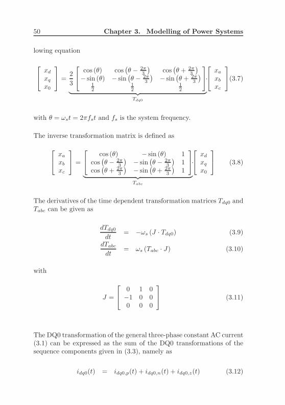
50 Chapter 3. Modelling of Power Systems
lowing equation
xdxqx0
=2
3
cos (θ) cos(θ − 2π
3
)cos(θ + 2π
3
)
− sin (θ) − sin(θ − 2π
3
)− sin
(θ + 2π
3
)
12
12
12
︸ ︷︷ ︸
Tdq0
·
xaxbxc
(3.7)
with θ = ωst = 2πfst and fs is the system frequency.
The inverse transformation matrix is defined as
xaxbxc
=
cos (θ) − sin (θ) 1cos(θ − 2π
3
)− sin
(θ − 2π
3
)1
cos(θ + 2π
3
)− sin
(θ + 2π
3
)1
︸ ︷︷ ︸
Tabc
·
xdxqx0
(3.8)
The derivatives of the time dependent transformation matrices Tdq0 andTabc can be given as
dTdq0dt
= −ωs (J · Tdq0) (3.9)
dTabcdt
= ωs (Tabc · J) (3.10)
with
J =
0 1 0−1 0 00 0 0
(3.11)
The DQ0 transformation of the general three-phase constant AC current(3.1) can be expressed as the sum of the DQ0 transformations of thesequence components given in (3.3), namely as
idq0(t) = idq0,p(t) + idq0,n(t) + idq0,z(t) (3.12)

3.4. DQ0 Representation 51
with
idq0,p(t) = Ip
cos(θp)sin(θp)0
(3.13)
idq0,n(t) = In
cos(2ωst+ θn)− sin(2ωst+ θn)0
(3.14)
idq0,z(t) = Iz
00cos(ωst+ θz)
(3.15)
After the analytical review of the DQ0 transformation and transformedgeneral quantities, we will consider their simulation performance underdifferent system conditions.
One of the advantages in analyzing the power system with symmetricalcomponents in DQ0 reference frame is that under balanced steady-stateoperation the electrical quantities have constant values. If the powersystem is at balanced steady-state, the steady-state current containsonly the positive sequence component idq0,p, which is time independentand constant. For other modes of balanced operation, such as duringelectromechanical oscillations, these quantities vary slowly with time(maximum 2-3 Hz). For balanced operation, the frequency content ofthe transients will be centered around DC, which is also the aim ofthe aforementioned baseband representation. This leads also to fastersimulation times under balanced conditions, as the variation of vari-ables in the DQ0 reference frame are much slower than the originalvariables in the three-phase ABC reference frame or even constant atsteady-state. Therefore in some programs (e.g. SIMPOW [7]) the DQ0transformation is applied to all components in the system. All variablesand equations of the models in the three-phase ABC reference frameare transformed to the DQ0 reference frame.
The DQ0 transformation is a single reference frame transformation asthe reference frame rotates with system frequency. Therefore the sim-ulations in the DQ0 reference frame will be efficient around systemfrequency, which is the case in balanced symmetrical systems.
But if there are unbalanced conditions in the system or other harmon-ics, this efficiency can decrease drastically. If the three-phase current

52 Chapter 3. Modelling of Power Systems
is unbalanced, it contains all three sequence components (idq0,p, idq0,nand idq0,z). Under unbalanced conditions, the frequency content of thetransients will be centered not only around DC but also around 2ωsdue to negative sequence quantities and around ωs due to zero sequencequantities. As mentioned before, this decreases the simulation perfor-mance drastically as the maximum occurring frequency in the basebandsignal is increased. The same disadvantage was also mentioned for thebaseband represented signals in Section 3.3. Unbalanced conditions orasymmetrical components however do not cause such harmonics in theABC reference frame. These harmonics with 2ωs and ωs during un-balanced conditions are inherent to the DQ0 representation of positive,negative, and zero sequence quantities.
3.5 Dynamic Phasor Representation
Irrespective of the chosen variable representation, there is always a pe-riodicity in the system quantities at steady-state. In the ABC repre-sentation the periodicity is with system frequency ωs regardless of thesystem conditions (balanced/unbalanced). In the DQ0 representation,depending on the sequence component of the signal, the negative se-quence quantities have a periodicity with double system frequency 2ωs,zero sequence quantities a periodicity with system frequency ωs. Thepositive sequence quantities are DC-quantities at steady-state, whichbrings significant advantages in simulating symmetrical power systemsunder balanced conditions. The disadvantages of the baseband repre-sentation and the DQ0 representation arise if the frequency content ofthe transformed quantities are not centered around a carrier frequency.In such cases, the baseband signals are not narrow banded but ratherwide banded. In this section, the focus will be on an analytical tool try-ing to overcome this problem by a Fourier approximation of the systemquantities.
The frequency spectrum of power system transients in the ABC refer-ence frame mostly contains frequency components which are centeredaround system frequency ωs. But the usage of power electronic baseddevices such as FACTs or HVDC give rise to other harmonics in thesystem due to the periodically switched mode of operation of these de-vices. In the DQ0 reference frame (even without power electronic baseddevices) high frequency components are not only centered around DC

3.5. Dynamic Phasor Representation 53
−3ωs −2ωs −ωs 0 ωs +2ωs +3ωs
ω
X(ω)
X−3(jω) X
−2(jω) X−1(jω) X0(jω) X1(jω) X2(jω) X3(jω)
Figure 3.7: Illustrative spectrum of power system transients
but also around double system frequency depending on the sequencecomponent (positive,negative or zero sequence). The half-band widthof these spectra is generally less than the system frequency. If the spec-trum of the transients is not condensed around the system frequency,but also around other harmonics, the advantages of baseband represen-tation disappears, as the maximum frequency of baseband signal is alsoincreased. Due to the Nyquist criterion, this has also a direct effect onthe maximum permissible step size during simulation.
In such cases the spectrum of the power system transients can be ap-proximated as illustrated in Figure 3.7 If the frequency contents of thetransients are centered around kωs with their half bandwidth less thanωs, the overall spectrum is a disjunctive combination of the spectraaround kωs (Xk(jω)).
X(jω) =
+∞∑
k=−∞Xk(jω)
As the spectral content Xk(jω) is the frequency shifted version of thebaseband signal Xk(jω), meaning Xk(jω) = Xk(jω− jkωs), the overallspectrum can be expressed as the sum of frequency shifted spectra ofanalytical baseband signals.
X(jω) =
+∞∑
k=−∞Xk(jω − jkωs)
With the inverse transformation from frequency domain to the time

54 Chapter 3. Modelling of Power Systems
domain, the signal x(t) becomes
x(t) =
+∞∑
k=−∞Xk(t) e
jkωst
where Xk(t) is the analytical baseband signal. Thus the signal x(t) isfully defined by the baseband signal Xk(t).
This approach can be also seen as a modified form of the Fourier seriesrepresentation of a periodic signal. A possibly complex valued periodicsignal with period T [ e.g. x(τ) = x(τ − T ) ] can be expressed with aFourier series representation of the form given by
x(τ) =
∞∑
k=−∞Xk e
j k ωs τ
where ωs = 2π/T and Xk is the kth Fourier coefficient in complex form.It is important to note, that as the signal x(τ) is periodic the Fouriercoefficients Xk are time invariant.
In power system steady-state analysis, these Fourier coefficients Xk arealso referred to as phasors. During transients, the system is not in apure periodic but nearly periodic state. The idea is now to extend thisapproach to nearly periodic signals [13] and to approximate x(τ) in theinterval τ ∈ (t − T, t] with a Fourier series representation of the formgiven in (3.16).
x(τ) =
∞∑
k=−∞Xk(t) e
j k ωs τ (3.16)
In this representation, as the signal x(τ) is nearly periodic and sincethe interval under consideration slides as a function of time, the Fouriercoefficients Xk are time varying. This expression can also interpretedas an orthogonal signal expansion of the function x(t) with orthonormalbasis ejkωst. The corresponding coordinate Xk(t) belonging to ejkωst,can be determined by the following inner product of the original signalwith the corresponding basis signal ejkωst
Xk(t) =⟨x(t) , ejkωst
⟩= 〈x(t)〉k
which is determined by
Xk(t) =1
T
t∫
t−T
x(τ) e−j k ωs τdτ (3.17)

3.5. Dynamic Phasor Representation 55
These time varying Fourier coefficients, which are equivalent to the an-alytical baseband signals in the previous representation, are referred toas dynamic phasors. Throughout the thesis, this methodology is calledthe Dynamic Phasors Approach.
In the dynamic phasors approach, we are interested in cases where only afew coefficients provide a good approximation of the original waveform.
x(t) ≈∑
k∈KXk(t) e
j k ωs t (3.18)
where K is the set of Fourier coefficients approximating the originalwaveform. As notation, here lowercase letters x(τ) are used for in-stantaneous variables and uppercase letters Xk(t) for dynamic phasors.Some important properties of dynamic phasors are:
• The relation between the derivatives of x(τ) and the derivatives ofXk(t), which is given in (3.19), where the time argument t has beenomitted for clarity. This can easily be verified by differentiatingthe formula given in (3.16)
⟨dx
dt
⟩
k
=dXk
dt+ j k ωsXk (3.19)
• The product of two time-domain variables equals a discrete timeconvolution of the two dynamic phasor sets of the variables, whichis given in (3.20).
〈x y〉k =
∞∑
l=−∞(Xk−l Yl) (3.20)
• For a complex valued signal x, the relationship between Xk andX−k is given as:
X−k = (X∗)k∗
(3.21)
where X∗k means the conjugate complex of Xk. For a real valued
signal, this property becomes
X−k = Xk∗ (3.22)

56 Chapter 3. Modelling of Power Systems
In the used simulation framework, the continuous dynamic behaviorof the power system components is described by Differential AlgebraicEquations
dx
dt= f(x, y)
0 = g(x, y) (3.23)
Using the appropriate approximations for the dynamic states x andalgebraic states y in (3.16) and the properties (3.19-3.20), we can ap-proximate the set of f and g equations of the model with a new set ofequations and get the definition of the dynamic phasor model in a newset of functions F and G as
dXk
dt= Fk(Xk, Yk) − j k ωsXk
0 = Gk(Xk, Yk) (3.24)
where the dynamic phasors Xk become the new continuous dynamicstates and Yk the new algebraic states.
The dynamic phasors approach offers a numbers of advantages overconventional methods.
+ The selection of set K gives a wider bandwidth in the frequencydomain than the traditional slow quasi-stationary assumptionsused in Transient Stability Programs, where the electromagnetictransients are totally neglected.
+ As the dynamic phasors Xk are all narrow banded baseband sig-nals, they can be numerically computed more efficiently.
+ The time domain simulations of such large systems with period-ically switched power electronic based components not only fea-ture a significant computational burden, but also give little insightinto the problem sensitivities to design controllers or protectionschemes. The dynamic phasors approach also allows an analyti-cal insight into such problems, as it approximates a periodicallyswitched system with a continuous system.
– One disadvantage of the dynamic phasors approach is that thenumber of variables and equations in the phasor dynamics ap-proach (3.24) is higher than in the original equations (3.23), which

3.6. Summary 57
can make the simulation inefficient. But the efficiency gain due toslower variations in the Fourier coefficients is mostly higher thanthe efficiency loss due to the increased number of variables andequations.
The dynamic phasors approach is based on an adequate approximationof the system variables and equations, whereas the DQ0 reference framerepresentation or the analytical baseband representation are based ontransformations. Thus great care must be taken in the selection of theapproximating signal space K to reflect the correct system behavior inthe application of the dynamic phasor approach.
For example in the case of the DQ0 reference frame in (3.12), an appro-priate selection for the approximation would be K = {0, 1, 2} as unbal-anced conditions induce terms with double system frequency (k = 2)in negative sequence and terms with system frequency (k = 1) in zerosequence.
In fact the dynamic phasors approach can be applied to both variablerepresentations in ABC and in DQ0 as the dynamic phasors approachis a general analytical tool. One advantage of the DQ0 based dynamicphasor model is the achieved decoupling of the sequence quantities withK = {0, 1, 2} which is an important property of the DQ0 transforma-tion. In ABC-based dynamic phasor models, this is not the case.
The dynamic phasors approach has been successfully employed to modelelectric machines, FACTS devices and power converters [17, 18, 14, 15].Our aim in this thesis is to use the dynamic phasor representation asa system representation in our simulator where the models are derivedbased on this approach and compare their simulation efficiency andaccuracy to other commonly used modelling techniques.
3.6 Summary
In this chapter, we discussed different variable representations used inpower systems modelling and power systems analysis . The main focuswas on their advantages and disadvantages from the simulation perfor-mance point of view.

58 Chapter 3. Modelling of Power Systems
• Three-phase ABC Representation: The three-phase ABCrepresentation provides a basis for the other derived variable rep-resentations. Important advantages and disadvantages are:
+ As instantaneous quantities are used, any kind of equipmentcan be modelled with this approach (e.g. detailed simulationpower electronic based devices).
+ As it takes the true physical model the simulations are accu-rate.
− For large power systems, the simulations can be inefficient asall components are modelled in detail and the instantaneousquantities are used for simulation.
• Baseband ABC Representation: In this representation, thebandpass real valued instantaneous quantities are transformed tobaseband complex valued quantities, which can be simulated moreefficiently i.e. with larger step sizes. Important advantages anddisadvantages are:
+ As the frequency contents of the quantities are only shiftedin the frequency domain, the models are still accurate.
+ The transformed quantities can be simulated more efficientlyas the variations in the baseband signal are much slower thanin the instantaneous quantities.
− If the frequency content of the instantaneous values are notconcentrated around the system frequency, this latter advan-tage disappears.
• DQ0 Representation: The aim of the DQ0 representation is toobtain an orthogonal and baseband representation of the originalABC quantities.
+ The models in DQ0 reference frame also give accurate results,since these models are derived by a transformation and notan approximation.
+ Simulations with these models are efficient if the system is ina balanced condition. In this case, only the positive sequencenetwork is simulated. The variations of the DQ0 transformedpositive sequence quantities are much slower than the instan-taneous values of the quantities in ABC reference frame, sothat they can be simulated with larger step sizes.

3.6. Summary 59
− However, if the system is in an unbalanced condition, neg-ative and zero sequence components occur in the system,with 2ωs and ωs oscillations. This makes the simulations in-efficient as the step size must be kept small enough to comeup with these oscillations.
− DQ0 transformation is a single reference frame transforma-tion. Thus it is only efficient at fundamental frequency ornear to fundamental frequency. If there are other harmonicsin the system (e.g. due to FACTS devices), this efficiencywill decrease drastically.
• Dynamic phasor models: In the dynamic phasors approach,the quantities are approximated with their time-varying Fouriercoefficients also named dynamic phasors. As these dynamic pha-sors have a baseband characteristic, they can be computed alsoefficiently.
+ The accuracy of the simulation is dependent on the appro-priate selection of Fourier coefficients K.
+ Simulations with phasor dynamics are efficient as we aresimulating Fourier coefficients and their variations are muchslower than the instantaneous values. Thus, simulations arefaster.
+ Dynamic phasors approach applied to power electronic de-vices transform the periodically switched system into a con-tinuous system, so that we gain more analytical insight (e.g.eigenvalue analysis).
− The number of the variables and equations can increase de-pending on the selection of K. This can decrease simulationperformance.
In the next chapter, we will derive the dynamic phasor models of somemajor components and will give a comparative assessment of the simula-tion performance of the described modelling techniques under balancedand unbalanced conditions. The comparison will regard the accuracyand efficiency under different operation conditions of the ABC, DQ0and dynamic phasor models.


Chapter 4
Comparative Assessment of
Different Modelling
Techniques
In the previous chapter we focused on the commonly used system vari-able representations in power system modelling and also introduced thedynamic phasors approach. In this chapter, we will derive the dynamicphasor models of major power system components and compare theirsimulation performance with others in the ABC and DQ0 referenceframe in terms of accuracy and computational efficiency.
4.1 Introduction
Chapter 3 dealt with the conventional system representations in powersystem modelling and analysis. Furthermore, the concept of dynamicphasors has been introduced where the instantaneous system quanti-ties are represented by their time varying Fourier coefficients. Thetheoretical evaluation of these system representations regarding theirsimulation performance under different operating conditions has beendiscussed by looking at their characteristics in the frequency domain.The conclusions we arrived at were more of a qualitative nature. In thisChapter, the aim is to justify these qualitative conclusions with quan-titative values by comparing the accuracy and computational efficiency
61

62 Chapter 4. Comparison of Modelling Techniques
of these modelling techniques in a systematic way. The consistency ofthis systematic comparison is warranted by implementing the differentlyrepresented models of major power system components and simulatingthem under different operating conditions using the same simulationframework. Details of the used simulation environment were given inChapter 2. Figure 4.1 illustrates the described aim of this Chapter.
DifferentModelling Techniques
DifferentOperating Conditions
Comparison ofaccuracy
SameSimulation framework
Comparison ofefficiency
Figure 4.1: Systematic comparison of different modelling techniques
The Chapter is structured as follows. First of all, dynamic phasor mod-els of major power system elements will be derived. In this Chapter,we will focus on the synchronous machine and the transmission linemodels for electromagnetic transients studies, since the used test case(Single Machine Infinite Bus-SMIB) contains these elements. Howeveralso dynamic phasor models of Thyristor-controlled Series Capacitorand Doubly-fed Induction machine are in the scope of the thesis. Thedynamic phasor model of the synchronous machine will be derived inthe conventionally used ABC and DQ0 reference frame.
Besides the detailed models of these components capturing fast elec-tromagnetic and slow electromechanical transients, we will also derivethe so called reduced order models capturing only the slower electrome-chanical transients. These reduced order models are equivalent to the

4.2. Transmission Line Model 63
fundamental frequency models used in transient stability studies.
As a test case, the SMIB system will be used under different operatingconditions namely, balanced and unbalanced conditions. Unbalancedfaults (e.g. single-line to ground fault) and asymmetrical componentswill be treated as unbalanced conditions. Finally the simulation perfor-mance of these dynamic phasor models will be compared with those inABC and DQ0.
4.2 Transmission Line Model
In this section, the dynamic phasor model of a simple transmission linewill be derived, where the equivalent circuit of each phase is representedby series RL branches with different R-L values and no mutual couplingsbetween the three phases. The dynamic phasor models will be based onmodel equations in the the original ABC phases and also in the DQ0reference frame. Hence, we will briefly treat the transmission line modelin the ABC and DQ0 reference frame and then accordingly derive thedynamic phasor models.
4.2.1 Dynamic Phasor Model − ABC
The per unit model equations of the above mentioned transmission linein the original ABC phases yield
dψabcdt
= vabc −Rabc iabc (4.1)
ψabc = Labc iabc (4.2)
with flux, voltage and current vectors
ψabc =[ψa (t) ψb (t) ψc (t)
]T
vabc =[va (t) vb (t) vc (t)
]T
iabc =[ia (t) ib (t) ic (t)
]T
The time argument (t) has been dropped in the electrical quantitiesψabc(t), vabc(t) and iabc(t). The square and diagonal inductance and

64 Chapter 4. Comparison of Modelling Techniques
resistance matrices Rabc and Labc are defined as
Rabc = diag[Ra Rb Rc
]
Labc = diag[La Lb Lc
]
Unequal resistance and inductance values for each phase have been usedto allow implementation of asymmetrical component models. For easeof formulation the mutual inductances have been ignored, but these caneasily be included in the model. Equation (4.1) provides the basis ofthe model equations for the hereafter derived transmission line models.
Now, we want to derive the dynamic phasor model of the transmissionline model given in (4.1). The first step is to decide on the approximat-ing Fourier coefficients set for the behavior of the model under balancedand unbalanced conditions. In other words, we first define the set ofdynamic phasor K in (3.18) used for the approximation.
In the case of the transmission line model given in (4.1) an appropriateselection for K would be K = {1}, since the currents and voltagesin the ABC phases are assumed to be sinusoidal or nearly sinusoidalwith system frequency. With this approximation and the properties(3.19-3.22), the dynamic phasor model of the transmission line in theABC phases with K = {1} from (4.1) can be derived as follows. WithK = {1}, the model equation (4.1) becomes
⟨dψabcdt
⟩
1
= 〈vabc〉1 − 〈Rabc iabc〉1〈ψabc〉1 = 〈Labc iabc〉1
Applying the rules (3.19-3.22) for the derivative and product, yields
d〈ψabc〉1dt
= 〈vabc〉1 −Rabc 〈iabc〉1 − j ωs 〈ψabc〉1 (4.3)
〈ψabc〉1 = Labc 〈iabc〉1 (4.4)
The model given in (4.3-4.4) is the EMT equivalent dynamic phasormodel capturing electromagnetic transients. In transient stability anal-ysis, the network transients are commonly neglected. Neglecting thenetwork transients would mean neglecting the variations in the dynamic
phasor 〈ψabc〉1 by settingd〈ψabc〉1
dt= 0. Thus, the model reflects only

4.2. Transmission Line Model 65
Variable Approximation K = {. . .}ψabc {1}vabc {1}iabc {1}
Parameters Approximation K = {. . .}Rabc constant
Labc constant
Table 4.1: Appropriate approximation for variables and parameters ofthe transmission line model with DPA
the steady state impedance relation between voltage phasor 〈vabc〉1 andcurrent phasor 〈iabc〉1, namely .
〈vabc〉1 = 〈iabc〉1 (Rabc + jωsLabc)
4.2.2 Dynamic Phasor Model − DQ0
Using the DQ0 or Park’s transformation, described in Section 3.4, themodel equations (4.1) can be transformed into the following form usingproperties (3.7) and (3.9)
dψdq0dt
= vdq0 −Rdq0 idq0 − ωs J ψdq0 (4.5)
ψdq0 = Ldq0 idq0 (4.6)
with flux, voltage and current vectors
ψdq0 = Tdq0 ψabc = [ ψd (t) ψq (t) ψ0 (t) ]T
vdq0 = Tdq0 vabc = [ vd (t) vq (t) v0 (t) ]T
idq0 = Tdq0 iabc = [ id (t) iq (t) i0 (t) ]T
J given in equation (3.11) and the time dependent and non-diagonalinductance and resistance matrices Ldq0(θs) and Rdq0(θs), with θs =ωs t and ωs the system frequency. The expression for Ldq0(θs) is givenas
Ldq0 (θs) = Tdq0 (θs) · Labc · Tabc (θs)
=
[Ldq (θs) Ldq,0 (θs)L0,dq (θs) L0
]
(4.7)

66 Chapter 4. Comparison of Modelling Techniques
with the following definitions
Ldq = ℜ{〈Ldq〉0 + 〈Ldq〉2 ej2θs
}(4.8)
Ldq,0 = ℜ{〈Ldq,0〉1 e
jθs}
(4.9)
L0,dq = ℜ{〈L0,dq〉1 e
jθs}
(4.10)
L0 = L0 (4.11)
〈Ldq〉0 =
[Lγ 00 Lγ
]
, 〈Ldq〉2 =1
3
[Lα jLαjLα −Lα
]
〈Ldq,0〉1 =1
3
[2Lβ2jLβ
]
, 〈L0,dq〉1 =1
3
[Lβ jLβ
], 〈L0〉0 = Lγ
Lγ =1
3La +
1
3Lb +
1
3Lc
Lα =2
3La −
1
3Lb −
1
3Lc =
1
3ℜ{
La + Lbej 2π
3 + Lce−j 2π
3
}
Lβ =1
3
√3 (Lc − Lb) =
1
3ℑ{
La + Lbej 2π
3 + Lce−j 2π
3
}
The resistance matrix Rdq0 also has the same form.
After grouping the dq0 coordinates of the quantities xdq0 and parame-ters into xdq and x0 coordinates, the model equations become
dψdqdt
= vdq −Rdq idq −Rdq,0 i0 − ωs J2 ψdq (4.12)
dψ0
dt= v0 −R0,dq idq −R0 i0 (4.13)
ψdq = Ldq idq + Ldq,0 i0 (4.14)
ψ0 = L0,dq idq + L0 i0 (4.15)
with
J2 =
[0 1−1 0
]
(4.16)
It is important to note the periodic time dependence of Ldq due to thee2jθs term and of Ldq,0, L0,dq due to the ejθs term in case of the DQ0transformed asymmetrical transmission line model.
In the case of a symmetrical line with La = Lb = Lc, Ldq0 becomesdiagonal and time independent as Lα = 0, Lβ = 0 and Lγ = La, which

4.2. Transmission Line Model 67
significantly simplifies the model equation (4.12) in the DQ0 referenceframe. Already this simple example shows that the DQ0 transforma-tion is advantageous only in conjunction with symmetrical componentssince asymmetrical conditions in the components induce time dependentparameters.
In the case of a symmetrical transmission line in the DQ0 referenceframe, the model inductance matrix Ldq is constant and diagonal, Ldq,0and L0,dq are zero. Assuming an asymmetrical transmission line, thesemodel inductance matrices will not be constant but time dependent dueto the periodic terms with ejθs , e2jθs as stated in (4.12-4.15). In thiscase for an asymmetrical transmission line the appropriate approxima-tion for the model parameters Ldq, Rdq will be K = {0, 2}, for Ldq,0,L0,dq, Rdq,0, R0,dq it will be K = {1} when deriving the correspondingdynamic phasor model in the DQ0 reference frame.
As discussed in Section 3.4, in the case of unbalanced conditions, whereall three sequence components (positive, negative and zero sequence) arepresent, the DQ0 transformed sequence components will appear withdifferent frequencies in the DQ0 reference frame. Under unbalancedconditions, the frequency content of the positive sequence quantities willbe centered around DC and that of the negative sequence quantities willbe around 2ωs. Both positive and negative sequence components willbe observed in the d and q axis but at different frequencies (i.e. around0 and 2ωs). The zero sequence components will only be observed in the0 axis and at frequencies around ωs.
Hence, in the case of unbalanced conditions, the appropriate set of ap-proximating Fourier coefficients for the transformed phase quantities inthe DQ0 frame are K = {0, 2} for the dq-coordinates and K = {1} forthe 0 -coordinate.
Table 4.2 shows the appropriate set of approximating set of Fouriercoefficients for the dynamic phasor transmission line model in the DQ0reference frame. Since the phase quantities in the DQ0 reference frameare also real valued, the positive indexed dynamic phasors e.g. K ={0, 1, 2} contain all the information about these quantities (3.22).
With the approximations given in Table 4.2 for electrical quantities andmodel parameters, the dynamic phasor model of the transmission line

68 Chapter 4. Comparison of Modelling Techniques
Quantity Condition Approximation K = {. . .}ψdq, vdq, idq Balanced {0}ψ0, v0, i0 Balanced −ψdq, vdq, idq Unbalanced {0, 2}ψ0, v0, i0 Unbalanced {1}Parameter Condition Approximation K = {. . .}Rdq, Ldq Symmetrical {0}R0, L0 Symmetrical {0}
Rdq,0, R0,dq Symmetrical −Ldq,0, L0,dq
Rdq, Ldq Asymmetrical {0, 2}R0, L0 Asymmetrical {0}
Rdq,0, R0,dq Asymmetrical {1}Ldq,0, L0,dq
Table 4.2: Appropriate approximation for variables and parameters ofthe transmission line model with DPA in the DQ0 referenceframe
in the DQ0 reference frame can be given as
⟨dψdqdt
⟩
0
= 〈vdq〉0 − 〈Rdq idq〉0 − 〈Rdq,0 i0〉0 − ωs J2 〈ψdq〉0⟨dψdqdt
⟩
2
= 〈vdq〉2 − 〈Rdq idq〉2 − 〈Rdq,0 i2〉2 − ωs J2 〈ψdq〉2⟨dψ0
dt
⟩
1
= 〈v0〉1 − 〈R0,dq idq〉1 − 〈R0 i0〉1〈ψdq〉0 = 〈Ldq idq〉0 + 〈Ldq,0 i0〉0〈ψdq〉2 = 〈Ldq idq〉2 + 〈Ldq,0 i2〉2〈ψ0〉1 = 〈L0,dq idq〉1 + 〈L0 i0〉1
With the properties regarding the derivative, product and conjugatecomplex of dynamic phasors (3.19-3.22), the dynamic phasor model of

4.2. Transmission Line Model 69
the transmission line yields
d〈ψdq〉0dt
= 〈vdq〉0 − 〈Rdq〉0 〈idq〉0 − 〈Rdq〉2 〈idq〉∗2 − 〈Rdq〉∗2 〈idq〉2
−〈Rdq,0〉1 〈i0〉∗1 − 〈Rdq,0〉∗1 〈i0〉1 − ωs J2 〈ψdq〉0 (4.17)
d〈ψdq〉2dt
= 〈vdq〉2 − 〈Rdq〉2 〈idq〉0 − 〈Rdq〉0 〈idq〉2−〈Rdq,0〉1 〈i0〉1 − ωs J2 〈ψdq〉2 (4.18)
d〈ψ0〉1dt
= 〈v0〉1 − 〈R0,dq〉1 〈idq〉0 − 〈R0,dq〉∗1 〈idq〉2−〈R0〉0 〈i0〉1 (4.19)
〈ψdq〉0 = 〈Ldq〉0 〈idq〉0 + 〈Ldq〉2 〈idq〉∗2 + 〈Ldq〉∗2 〈idq〉2
+〈Ldq,0〉1 〈i0〉∗1 + 〈Ldq,0〉∗1 〈i0〉1 (4.20)
〈ψdq〉2 = 〈Ldq〉2 〈idq〉0 + 〈Ldq〉0 〈idq〉2 + 〈Ldq,0〉1 〈i0〉1 (4.21)
〈ψ0〉1 = 〈L0,dq〉1 〈idq〉0 + 〈L0,dq〉∗1 〈idq〉2 + 〈L0〉0 〈i0〉1 (4.22)
The parameters 〈Ldq〉k, 〈Ldq,0〉k, 〈L0,dq〉k and 〈L0〉k correspond to theexpressions given in (4.8-4.11). Compared with the original model equa-tions in the DQ0 reference frame, the dynamic phasor model inductancesand resistances are constant in contrast to those represented with in-stantaneous quantities in the DQ0 reference frame. However comparedwith dynamic phasor model equations in the ABC reference frame, thedynamic phasor model equations in the DQ0 reference frame are morecomplicated.
In the case of a symmetrical transmission line model, the parameters〈Ldq,0〉1, 〈L0,dq〉1 and 〈Ldq〉2 become zero. This simplifies the modelequations significantly.
d〈ψdq〉0dt
= 〈vdq〉0 − 〈Rdq〉0 〈idq〉0 − ωs J2 〈ψdq〉0 (4.23)
d〈ψdq〉2dt
= 〈vdq〉2 − 〈Rdq〉0 〈idq〉2 − ωs J2 〈ψdq〉2 (4.24)
d〈ψ0〉1dt
= 〈v0〉1 − 〈R0〉0 〈i0〉1 (4.25)
〈ψdq〉0 = 〈Ldq〉0 〈idq〉0 (4.26)
〈ψdq〉2 = 〈Ldq〉0 〈idq〉2 (4.27)
〈ψ0〉1 = 〈L0〉0 〈i0〉1 (4.28)
The formulation of the asymmetrical transmission line dynamic phasor

70 Chapter 4. Comparison of Modelling Techniques
model in the DQ0 components is computationally not that efficient dueto the increased complexity.
The transmission line model defined with the equations (4.12-4.15) is theEMT equivalent model in the DQ0 reference frame with instantaneousvalues. The equivalent fundamental frequency models for transient sta-bility studies assume generally that the fast electromagnetic transientshave decayed and the electrical quantities have reached their steadystate values. The fundamental frequency model derivation is generallyaccomplished by setting the derivative of the electrical quantities equalto zero if the steady state values of these quantities are DC quantities.Hence, this can only be applied to the equations (4.12-4.15) if and onlyif the system is under balanced conditions. Since the system is underbalanced conditions, it will only contain positive sequence components,which get constant in the DQ0 reference frame at balanced steady state.For unbalanced steady state conditions, setting the derivative to zerowill not be valid, since the negative sequence components will have os-cillations with 2ωs and zero sequence components with ωs.
In contrast to the representations with the instantaneous values in theDQ0 reference frame, the steady state values of dynamic phasors in theDQ0 reference frame are constant even under unbalanced conditions.This allows a systematic derivation of reduced order models for transientstability studies, just by setting the derivatives of the dynamic phasorsof the network quantities to zero. Hence the dynamic phasor modelof the transmission line used for transient stability analysis where theelectromagnetic transients are neglected, can be derived by setting thed〈ψdq〉k
dt=
d〈ψ0〉k
dt= 0 in the model equations (4.17-4.19).
4.3 Synchronous Machine
The modelling of synchronous machines has been a primary researchtopic in power system engineering for several years. Today there are alarge number of different models used in different studies. Hence, thechoice of the correct model highly depends on the frequency range of thestudy. In this section, we will base our dynamic phasor model on the thesynchronous machine representation described in Chapter 3 in [33]. Thisrepresentation is commonly used in electromagnetic transients studiesand also in transient stability analysis. In this part of the chapter,

4.3. Synchronous Machine 71
starting with the synchronous machine equations in the ABC and DQ0reference frame, the dynamic phasor model of the synchronous machinewill be derived in both reference frames. In [17] a similar derivation wasmade based on the space vector representation. Here we will use theDQ0 representation of the model equations.
4.3.1 Dynamic Phasor Model − ABC
The synchronous machine under consideration has one damper windingin the D-axis, two damper winding in the Q-axis and a field wind-ing. The notation and formulae for describing the synchronous machinemodel are adopted from [33]. The following assumptions are made forthe model derivation
• The stator currents are assumed to be positive when they flow outof the machine.
• The rotor currents are assumed to be positive when they flow intothe machine.
• The direct axis (d-axis) is centered magnetically in the center ofthe north pole
• The quadrature axis (q-axis) leads the direct axis by 90◦ electricaldegrees in the direction of rotation
The overall set of per unit model equations of the synchronous machineis generally divided into the voltage equations,
1
ωs
dψsdt
= es +Rss is (4.29)
1
ωs
dψrdt
= er +Rrr ir (4.30)
the flux linkages equations between the stator/rotor windings,
ψs = Lss (θr) is + Lsr (θr) ir (4.31)
ψr = Lsr (θr) is + Lrr ir (4.32)

72 Chapter 4. Comparison of Modelling Techniques
and the mechanical equations describing the effect of the unbalancebetween the electromagnetic torque and the mechanical torque.
Te =2√
3
9[ia (ψc − ψb) + ib (ψa − ψc) + ic (ψb − ψa)] (4.33)
dωrdt
=1
2H(Tm−Te −KD ωr) (4.34)
1
ωs
dδrdt
= ωr−1 (4.35)
with the following definitions:
• ψ . . . the vector consisting of the per unit stator and rotor fluxes
• e . . . the vector consisting of the per unit stator and rotor voltages
• i . . . the vector consisting of the per unit stator and rotor currents
• Te . . . the per unit electrical torque
• Tm . . . the per unit mechanical torque
• ωs . . . the system frequency
• ωr . . . the per unit rotor speed
• δr . . . the rotor angle
• θr . . . the angle by which the direct axis leads the A-phase windingin the direction of rotation θr = ωs t+ δr
• R . . . the diagonal per unit resistance matrix
• L . . . the per unit inductance matrix
• H . . . the per unit inertia constant
• KD . . . the per unit damping factor

4.3. Synchronous Machine 73
Analytically one has
ψ = [ ψa ψb ψc︸ ︷︷ ︸
ψs
ψfd ψ1d ψ1q ψ2q︸ ︷︷ ︸
ψr
]T
i = [ −ia −ib −ic︸ ︷︷ ︸
is
ifd i1d i1q i2q︸ ︷︷ ︸
ir
]T
e = [ ea eb ec︸ ︷︷ ︸
es
efd 0 0 0︸ ︷︷ ︸
er
]T
R = diag[ Ra Ra Ra︸ ︷︷ ︸
Rss
Rfd R1d R1q R2q︸ ︷︷ ︸
Rrr
]T
The flux linkage for each generator winding is composed of a linkage dueto the stator windings and a linkage due to the windings on the rotor.Hence, the instantaneous flux linkage can be divided into two parts.
(ψsψr
)
︸ ︷︷ ︸
ψ
=
(Lss (θr) Lsr(θr)
Lrs (θr) Lrr
)
︸ ︷︷ ︸
L(θr)
(isir
)
︸ ︷︷ ︸
i
(4.36)
with Lss, Lrr being the self inductances of the stator and rotor wind-ings and Lsr, Lrs the mutual inductances between the stator and rotorwindings. The self inductances of the stator and rotor windings Lss,Lrr and the mutual inductances between the stator and rotor windingsLsr, Lrs are defined as
Lss =
La,a La,b La,cLb,a Lb,b Lb,cLc,a Lc,b Lc,c
Lrr =
Lf,f Lf,1d Lf,1q Lf,2qL1d,f L1d,1d L1d,1q L1d,2q
L1q,f L1q,1d L1q,1q L1q,2q
L2q,f L2q,1d L2q,1q Lq2q2
Lsr =
La,f La,1d La,1q La,2qLb,f Lb,1d Lb,1q Lb,2qLc,f Lc,1d Lc,1q Lc,2q
Lrs =
Lf,a Lf,b Lf,cL1d,a L1d,b L1d,c
L1q,a L1q,b L1q,c
L2q,a L2q,b L2q,c

74 Chapter 4. Comparison of Modelling Techniques
where the individual inductances are defined as follows:
La,a = Laa0 + Laa2 cos (2θr)
Lb,b = Laa0 + Laa2 cos
(
2θr −4π
3
)
Lc,c = Laa0 + Laa2 cos
(
2θr +4π
3
)
La,b = Lba = Lab0 + Laa2 cos(
2θr +π
3
)
La,c = Lca = Lab0 + Laa2 cos(
2θr −π
3
)
Lb,c = Lcb = Lab0 + Laa2 cos (2θr − π)
Lf,f = Lffd
L1d,1d = L1d
L1q,1q = L1q
L2q,2q = L2q
Lf,1d = L1,df = Lf1d
L1q,2q = L2q,1q = L12q
Lf,1q = Lf,2q = L1q,f = Lf,2q = 0
L1d,1q = L1q,1d = L1d,2q = L2q,1d = 0
La,f = Lf,a = Lafd cos (θr)
Lb,f = Lf,b = Lafd cos
(
θr −2π
3
)
Lc,f = Lf,c = Lafd cos
(
θr +2π
3
)
La,1d = L1d,a = La1d cos (θr)
Lb,1d = L1d,b = La1d cos
(
θr −2π
3
)
Lc,1d = L1d,c = La1d cos
(
θr +2π
3
)
La,1q = L1q,a = −La1q sin (θr)
Lb,1q = L1q,b = −La1q sin
(
θr −2π
3
)
Lc,1q = L1q,c = −La1q sin
(
θr +2π
3
)

4.3. Synchronous Machine 75
La,2q = L2q,a = −La2q sin (θr)
Lb,2q = L2q,b = −La2q sin
(
θr −2π
3
)
Lc,2q = L2q,c = −La2q sin
(
θr +2π
3
)
Since the rotor is rotating with the angular velocity ωr with respect tostator, the self and mutual inductances are not constant and depend onthe electric rotor position θr(t) with respect to the winding of phase A.The stator self inductance matrix Lss consists of a constant term andof a time dependent periodic term varying with 2 θr. The rotor/statormutual inductance matrices Lsr and Lrs are also time dependent andperiodic with θr. The rotor self inductance matrix Lrr is constant.Thus, the overall inductance matrix L can be expressed as
L (θr) = ℜ{(
Lss,0 + Lss,2ej 2 θr Lsr,1e
j θr
Lrs,1ej θr Lrr,0
)}
with
Lss,0 =
Laa0 Lab0 Lab0Lab0 Laa0 Lab0Lab0 Lab0 Laa0
Lrr,0 =
Lffd Lf1d 0 0Lf1d L11d 0 0
0 0 L11q L12q
0 0 L21q L22q
Lrs,1 = −LTsr,1 =
Lafd Lafd e−j 2π
3 Lafd ej 2π
3
La1d La1d e−j 2π
3 La1d ej 2π
3
j La1q j La1q e−j 2π
3 j La1q ej 2π
3
j La2q j La2q e−j 2π
3 j La2q ej 2π
3
Lss,2 = Laa2
1 e−j2π3 ej
2π3
e−j2π3 ej
2π3 1
ej2π3 1 e−j
2π3
Thus, with the equations (4.29-4.35) and the position dependent in-ductance matrix L (θr), the synchronous machine model equations withinstantaneous variables in the ABC reference frame are defined.

76 Chapter 4. Comparison of Modelling Techniques
Our aim is now to derive the dynamic phasor model based on this ABCreference frame representation. The derivation of the dynamic phasormodel requires an appropriate selection of the approximating Fouriercoefficients for the variables and parameters of the model. With ωs setas the fundamental frequency for the dynamic phasor approximationand considering θr(t) = θs(t) + δr(t) = ωs t+ δr(t), the time dependentinductance matrices Lss (θr), Lsr (θr), Lrs (θr) and Lrr can be expressedas
Lss (θr) = ℜ{〈Lss〉0 + 〈Lss〉2 ej2θs
}
Lrs (θr) = ℜ{〈Lsr〉1 ejθs
}
Lsr (θr) = ℜ{〈Lrs〉1 ejθs
}
Lrr (θr) = ℜ{〈Lrr〉0}
with
〈Lss〉0 = Lss,0 , 〈Lss〉2 = Lss,2 ej2δr
〈Lsr〉1 = Lsr,1 ejδr , 〈Lrs〉1 = Lrs,1 e
jδr
〈Lrr〉0 = Lrr
With these approximations, the variations in the inductance matrixL with θr(t) have been reduced to δr(t) during transients. At steadystate, the inductance matrix L becomes constant in the dynamic phasorrepresentation due to the constant rotor angle i.e. δr(t) = 0, whereasin the original three-phase ABC representation, the inductance matrixis still time dependent due to the synchronous speed θr(t) = ωs even insteady state.
Since unbalanced conditions are considered, the appropriate set of ap-proximating Fourier coefficients for stator quantities (denoted with thesubscript s) is Ks = {1} and for the rotor quantities (denoted with thesubscript r) Kr = {0, 2}. Table 4.3 shows the overall set of approxi-mating set of Fourier coefficients for the dynamic phasor model of thesynchronous machine in the ABC reference frame.
With the approximations given in Table 4.3 for the model variables andparameters, and the properties (3.19-3.22), the dynamic phasor modelof the synchronous machine in the ABC reference frame yields

4.3. Synchronous Machine 77
Quantity Approximation K = {. . .}ψs, es, is {1}ψr, er, ir {0, 2}Te, ωr, δr {0, 2}
Tm {0}Parameter Approximation K = {. . .}
Lss {0, 2}Lsr, Lrs {1}
Lrr, Rss, Rrr {0}
Table 4.3: Appropriate approximation for variables and parameters ofthe synchronous machine model with DPA in the ABC ref-erence frame
Voltage Equations:
1
ωs
d〈ψs〉1dt
= 〈es〉1 +Rss 〈is〉1 − j 〈ψs〉1 (4.37)
1
ωs
d〈ψr〉0dt
= 〈er〉0 +Rrr 〈ir〉0 (4.38)
1
ωs
d〈ψr〉2dt
= 〈er〉2 +Rrr 〈ir〉2 − j 2 〈ψr〉2 (4.39)
Flux Linkage Equations:
〈ψs〉1 = 〈Lss〉0 〈is〉1 + 〈Lss〉2 〈is〉∗1 + 〈Lsr〉1 〈ir〉0 + 〈Lsr〉∗1 〈ir〉2 (4.40)
〈ψr〉0 = 〈Lrs〉1 〈is〉∗1 + 〈Lrs〉∗1 〈is〉1 + 〈Lrr〉0 〈ir〉0 (4.41)
〈ψr〉2 = 〈Lrs〉1 〈is〉1 + 〈Lrr〉0 〈ir〉2 (4.42)
Mechanical Equations:
Te =2√
3
9
[
〈ia〉1(〈ψc〉∗1 − 〈ψb〉∗1
)+ 〈ia〉∗1 (〈ψc〉1 − 〈ψb〉1)
+〈ib〉1(〈ψa〉∗1 − 〈ψc〉∗1
)+ 〈ib〉∗1 (〈ψa〉1 − 〈ψc〉1)
+〈ic〉1(〈ψb〉∗1 − 〈ψa〉∗1
)+ 〈ic〉∗1 (〈ψb〉1 − 〈ψa〉1)
]
(4.43)

78 Chapter 4. Comparison of Modelling Techniques
d〈ωr〉0dt
=1
2H(Tm − 〈Te〉0 −KD 〈ωr〉0) (4.44)
d〈ωr〉2dt
=1
2H(−〈Te〉2 −KD 〈ωr〉2) − j 2ωs 〈ωr〉2 (4.45)
1
ωs
d〈δr〉0dt
= (〈ωr〉0 − 1) (4.46)
1
ωs
d〈δr〉2dt
= 〈ωr〉2 − j 2 〈δr〉2 (4.47)
The dynamic phasor model described by the equations (4.37-4.47), cap-tures both electromagnetic and electromechanical transients. In tran-sient stability analysis, the electromagnetic network transients and thethe electromagnetic stator transients are generally disregarded. Theequivalent dynamic phasor model for transient stability analysis canbe derived by setting the stator flux transients to zero in (4.37) i.ed〈ψs〉1dt
= 0.
4.3.2 Dynamic Phasor Model − DQ0
The model equations of the synchronous machine are usually given inthe DQ0 reference frame rotating with the rotor speed ωr. One ofthe main advantages in treating the synchronous machine in the DQ0reference frame rotating the with the rotor speed is that the transformedinductance matrices Lss, Lsr, Lrs and Lrr yield constant terms. Thesame notation and formulae are used as in [33] for the model equations.The overall set of per unit model equations in the DQ0 reference frameare given by
Voltage Equations:
1
ωs
dψdqdt
= erdq +Rdq irdq − ωr J2 ψdq (4.48)
1
ωs
dψ0
dt= er0 +R0 i
r0 (4.49)
1
ωs
dψrdt
= er +Rrr ir (4.50)

4.3. Synchronous Machine 79
Flux Linkage Equations:
ψdq = Ldq irdq + Ldq,r ir (4.51)
ψ0 = L0 ir0 (4.52)
ψr = Lr,dq irdq + Lrr ir (4.53)
Mechanical Equations:
Te = ψd irq − ψq i
rd (4.54)
dωrdt
=1
2H(Tm−Te −KD ωr) (4.55)
1
ωs
dδrdt
= ωr−1 (4.56)
with J2 given in (4.16) and
ψ = [ ψd ψq︸ ︷︷ ︸
ψdq
ψ0 ψfd ψ1d ψ1q ψ2q︸ ︷︷ ︸
ψr
]T
i = [ −ird −irq︸ ︷︷ ︸
−irdq
−ir0 ifd i1d i1q i2q︸ ︷︷ ︸
ir
]T
e = [ erd erq︸ ︷︷ ︸
erdq
er0 efd 0 0 0︸ ︷︷ ︸
er
]T
R = diag[ Ra Ra︸ ︷︷ ︸
Rdq
Ra︸ ︷︷ ︸
R0
Rfd R1d R1q R2q︸ ︷︷ ︸
Rrr
]T
Ldq =
[Ld 00 Lq
]
, Ldq,r =
[Lafd La1d 0 0
0 0 La1q La2q
]
Lr,dq =
Lafd 0La1d 0
0 La1q0 La2q
, Lrr =
Lffd Lf1d 0 0Lf1d L11d 0 0
0 0 L11q L12q
0 0 L12q L22q
The stator voltages and currents in the DQ0 reference frame rotatingwith the rotor speed ωr are interfaced with the network equations repre-sented in the DQ0 reference frame rotating with the synchronous speedωs by the following transformation:
esdesqes0
=
cos(δr) − sin(δr) 0sin(δr) cos(δr) 0
0 0 1
erderqer0
(4.57)

80 Chapter 4. Comparison of Modelling Techniques
When we derive the dynamic phasor model of the synchronous machinein the DQ0 reference frame, the d- and q-axis coordinates of the statorside electrical quantities are approximated by K = {0, 2} due to thepositive (k = 0) and negative (k = 2) sequence components and the0-axis coordinates by K = {1} due to the zero sequence component.The rotor side electrical quantities are approximated by K = {0, 2} aswas the case also in the ABC reference frame. The appropriate set ofthe approximating Fourier coefficients for the variables and parametersof the dynamic phasor model of the synchronous machine in the DQ0reference frame are given in Table 4.4. With the approximations inTable 4.4, the dynamic phasor model equations yield
Quantity Approximation K = {. . .}ψdq, idq, edq {0, 2}ψ0, i0, e0 {1}ψr, ir, er {0, 2}Te, ωr, δr {0, 2}
Tm {0}Parameter Approximation K = {. . .}
Lss, Ldq,r, Lr,dq, Lrr, Rss,Rrr -
Table 4.4: Set of approximations for the variables and parameters ofthe synchronous machine model in the DQ0 reference frame
Voltage Equations:
1
ωs
d〈ψdq〉0dt
=⟨erdq⟩
0+Ra
⟨irdq⟩
0(4.58)
+J2
(〈ωr〉0 〈ψdq〉0 + 〈ωr〉2 〈ψdq〉
∗2 + 〈ωr〉∗2 〈ψdq〉2
)
1
ωs
d〈ψdq〉2dt
=⟨erdq⟩
2+Ra
⟨irdq⟩
2(4.59)
+J2
(〈ωr〉0 〈ψdq〉2 + 〈ωr〉2 〈ψdq〉
∗0
)− j 2 〈ψdq〉2
1
ωs
d〈ψ0〉1dt
= 〈er0〉1 +Ra 〈ir0〉1 − j 〈ψ0〉1 (4.60)
1
ωs
d〈ψr〉0dt
= 〈er〉0 +Rrr 〈ir〉0 (4.61)
1
ωs
d〈ψr〉2dt
= 〈er〉2 +Rrr 〈ir〉2 − j 2 〈ψr〉2 (4.62)

4.3. Synchronous Machine 81
Flux Linkage Equations:
〈ψdq〉0 = Ldq⟨irdq⟩
0+ Ldq,r 〈ir〉0 (4.63)
〈ψdq〉2 = Ldq⟨irdq⟩
2+ Ldq,r 〈ir〉2 (4.64)
〈ψ0〉1 = L0 〈ir0〉1 (4.65)
〈ψr〉0 = Ldq,r⟨irdq⟩
0+ Lrr 〈ir〉0 (4.66)
〈ψr〉2 = Ldq,r⟨irdq⟩
2+ Lrr 〈ir〉2 (4.67)
Mechanical Equations:
〈Te〉0 = 〈ψd〉0⟨irq⟩
0+ 〈ψd〉2
⟨irq⟩∗2
+ 〈ψd〉∗2⟨irq⟩
2
−〈ψq〉0 〈ird〉0 − 〈ψq〉2 〈i
rd〉∗2 − 〈ψq〉∗2 〈i
rd〉2 (4.68)
〈Te〉2 = 〈ψd〉0⟨irq⟩
2+ 〈ψd〉2
⟨irq⟩
0
−〈ψq〉0 〈ird〉2 − 〈ψq〉2 〈i
rd〉0 (4.69)
d〈ωr〉0dt
=1
2H(Tm − 〈Te〉0 −KD 〈ωr〉0) (4.70)
d〈ωr〉2dt
=1
2H(−〈Te〉2 −KD 〈ωr〉2) − j 2ωs 〈ωr〉2 (4.71)
1
ωs
d〈δr〉0dt
= 〈ωr〉0 − 1 (4.72)
1
ωs
d〈δr〉2dt
= 〈ωr〉2 − j 2 〈δr〉2 (4.73)
The equivalent dynamic phasor model for transient stability analysiscan be derived by setting the stator flux transients in the DQ0 reference
frame to zero in (4.58-4.60) i.ed〈ψdq〉0dt
=d〈ψdq〉2dt
=d〈ψ0〉1dt
= 0.
In Section 2.4, the Automatic Code Generator tool was implementedto facilitate the creation of models for the user. This tool has beenextended to facilitate also the creation of the dynamic phasor models.The so called Dynamic Phasor Model Creator takes the model definitionfile of the detailed time domain model in the ABC or DQ0 referenceframe together with the appropriate set of Fourier coefficients for eachstate of the model (e.g. Table 4.4) and creates the model definition file ofthe corresponding dynamic phasor model. This procedure is illustratedin Figure 4.2. All dynamic phasor models of the components discussedin this Section have been created using the described tool.

82 Chapter 4. Comparison of Modelling Techniques
M D Fodel efinition ile
in the ABC or DQOreference frame of the model
Dynamic Phasor Model Generator
Set of approximating Fouriercoefficients for the states
of the model
M D Fodel efinition ile of the Dynamic Phasor Model
in the ABC or DQO reference frame
Figure 4.2: Flow chart of the Tool for creating Dynamic Phasor Models
4.4 Test Cases
In this Section, the aim is to compare the accuracy and computationalefficiency of the different modelling techniques in a systematic way. Forthis purpose, the previously described models i.e.
• detailed time domain models in the ABC reference frame(EMT-ABC)
• detailed time domain models in the DQ0 reference frame(EMT-DQ0)
• dynamic phasor models in the ABC reference frame(DYNPH-EMT-ABC)
• dynamic phasor models in the DQ0 reference frame(DYNPH-EMT-ABC)
of major power system components have been implemented in the simu-lation framework described in Chapter 2. The labels in the parenthesisin the above list will be used as reference to the used modelling tech-nique in the following figures containing the simulation results.
As test case, we have used the Single Machine Infinite Bus (SMIB)system described in [33]. Figure 4.3 shows the single line diagram of thetest system. Simulations have been performed with the detailed modelsfor simulating the electromagnetic transients and with the reduced order

4.4. Test Cases 83
models for transient stability analysis. Comparisons have been doneregarding the accuracy and computational efficiency of these models.As a quantitative evaluation of the computational efficiency of thesemodels, the overall CPU simulation times have been compared. Theevaluation of the accuracy has been done in a more qualitative wayby comparing the plots of the system quantities in the figures, whichseemed to be enough for our purpose.
4.4.1 Unbalanced Faults
In this test case, a single-phase to ground fault occurs at the BUS2 endof the LINE3 at 0.011 seconds and is removed after 0.20 seconds bydisconnecting the line LINE3. Simulations were obtained using Matlab7.1 running on a Intel Pentium IV CPU with 3.80 GHz and 2 GB ofRAM. The trapezoidal method with an absolute tolerance atol = 10−3
and relative tolerance rtol = 10−4 has been used for the numericalintegration of the four test cases.
Detailed Models
Figure 4.4 shows the evolution of the dynamic phasor components 〈Te〉0and 〈Te〉2 of the electrical torque. We observe that the per unit dynamicphasor component with k = 0, i.e. 〈Te〉0, captures the positive sequenceelectrical torque of Te. The dynamic phasor component with k = 2, i.e.〈Te〉2, captures the negative sequence electrical torque of Te. This isonly present during unbalanced conditions which is shown in the zoomedsection of the Figure 4.4.
INFEEDLINE1
LINE2
LINE3
BUS3BUS2
GEN
BUS1
Figure 4.3: Single line diagram of the SMIB system

84 Chapter 4. Comparison of Modelling Techniques
Figures 4.5-4.7 show the evolution of the per unit fault phase current ia,per unit generator phase-A terminal current ia and per unit generatorelectrical torque Te, after the unbalanced fault. In these Figures thecorresponding instantaneous values of the quantities in the simulationswith the dynamic phasor models are used. They can be computed bythe following approximation:
x(t) ≈ ℜ{∑
k∈KXk(t) e
j k ωs t
}
where K represents the set of the approximating Fourier coefficientsused for the particular state or variable. For example the instantaneousvalue of the electrical torque Te simulated with the dynamic phasormodels can be approximated by
Te(t) ≈ 〈Te〉0 + ℜ{〈Te〉2} cos (2ωs t) −ℑ{〈Te〉2} sin (2ωs t)
Table 4.5 shows the required CPU simulation times for the overall sim-ulation with four different modelling techniques. Table 4.5 and Fig-ures (4.5-4.7) allow a fair comparison of the four different modellingtechniques, since simulations have been done with the same simula-tion framework using the same numerical integration technique with thesame degree of numerical accuracy i.e. atol = 10−3 and rtol = 10−4.
EMT-ABC EMT-DQ0 DYNPH-EMT-ABC DYNPH-EMT-DQ0
469.359 [s] 70.468 [s] 11.688 [s] 15.487 [s]
Table 4.5: CPU simulation times of the overall simulation with fourdifferent modelling techniques
If the four modelling techniques are compared regarding accuracy, allresults in Figures (4.5-4.7) are in overall agreement during the wholesimulation interval and also during the interval with the unbalancedsingle phase to ground fault, which is depicted in the zoomed section ofthe plots.
Figure 4.7 depicts the phase-A fault current ifaulta during the fault sim-ulated with four different modelling techniques. Generally the faultcurrent has two distinct components [33], a fundamental frequency com-ponent with a subtransient and a transient period and an unidirectional

4.4. Test Cases 85
Time [s]
〈Te〉 0
,〈T
e〉 2
[pu]
〈Te〉0ℜ{〈Te〉2
}
ℑ{〈Te〉2
}
Time [s]
〈Te〉 0
,〈T
e〉 2
[pu]
〈Te〉0ℜ{〈Te〉2
}
ℑ{〈Te〉2
}
0 0.02 0.04 0.06 0.08 0.1 0.12 0.14 0.16 0.18 0.2
0 0.5 1 1.5 2 2.5
-1.5
-1
-0.5
0
0.5
1
1.5
2
-1
-0.5
0
0.5
1
1.5
Figure 4.4: Overall evolution of the dynamic phasors K = {0, 2} of theper unit electrical torque Te of GEN1 after a single line toground fault at BUS2 simulated with the detailed dynamicphasor models in the ABC reference frame. The zoomedsection shows the evolution during the unbalanced fault.
component which decays exponentially in several cycles. The unidirec-tional component occurs due to fact that stator fluxes cannot changeinstantaneously, so that this produces the dc offset in the phase cur-rents. This dc-component and the fundamental frequency componentof the fault current is also evident in the simulations with the dynamicphasor models.
We can conclude that the accuracy of the modelling techniques arenearly the same in all four cases. But if the comparison is made regard-ing the computational efficiency as shown in Table 4.5, the dynamicphasor models show a better performance than their counter parts with

86 Chapter 4. Comparison of Modelling Techniques
Time [s]
Te
[pu]
EMT-ABCEMT-DQ0DYNPH-EMT-ABCDYNPH-EMT-DQ0
Time [s]
Te
[pu]
0.02 0.04 0.06 0.08 0.1 0.12 0.14 0.16 0.18 0.2
0 0.5 1 1.5 2 2.5
-2
-1
0
1
2
3
-2
-1
0
1
2
3
Figure 4.5: Overall evolution of the per unit field current Te after asingle line to ground fault at BUS2 simulated with the fourdifferent detailed models. The zoomed section shows theevolution during the unbalanced fault.
the instantaneous values.
The instantaneous three-phase ABC models are computationally inef-ficient due to the permanent presence of the AC quantities even atsteady state, so that the highest frequency is always around the systemfrequency ωs, which affects the admissible maximum integration stepsize.
The instantaneous three-phase DQ0 models are computationally moreefficient than the instantaneous three-phase ABC models due to thedominating balanced operating conditions except during the unbalancedfault. After fast transients have decayed, the frequency content of theDQ0 transformed quantities will be located around DC during the bal-

4.4. Test Cases 87
Time [s]
i a[p
u]
EMT-ABCEMT-DQ0DYNPH-EMT-ABCDYNPH-EMT-DQ0
Time [s]
i a[p
u]
0 0.02 0.04 0.06 0.08 0.1 0.12 0.14 0.16 0.18 0.2
0 0.5 1 1.5 2 2.5
-6
-4
-2
0
2
4
-6
-4
-2
0
2
4
Figure 4.6: Overall evolution of the per unit generator terminal currentia after a single line to ground fault at BUS2 simulatedwith the four different detailed models. The zoomed sectionshows the evolution during the unbalanced fault.
anced conditions so that they can be integrated with larger step sizes in-creasing the simulation performance significantly. Due to the increasedcomputational efficiency during balanced conditions, the instantaneousmodels in the DQ0 reference frame are 6 times faster than those in theABC reference frame.
Both dynamic phasor models in the ABC and DQ0 reference frameare faster compared with the models with the instantaneous values.The variations in the dynamic phasors of the system quantities aremuch slower than in the instantaneous values of the quantities and theybecome constant at steady state. This fact does not depend on theselected reference frame. The selected reference has only an impact

88 Chapter 4. Comparison of Modelling Techniques
Time [s]
ifa
ult
a[p
u]
EMT-ABCEMT-DQ0DYNPH-EMT-ABCDYNPH-EMT-DQ0
Time [s]
ifa
ult
a[p
u]
EMT-ABCEMT-DQ0DYNPH-EMT-ABCDYNPH-EMT-DQ0
0.2022 0.2027 0.2032
0.02 0.04 0.06 0.08 0.1 0.12 0.14 0.16 0.18 0.2
4.9
4.92
4.94
4.96
4.98
5
5.02
5.04
-4
-2
0
2
4
6
8
10
12
Figure 4.7: The evolution of the per unit phase-A fault current ifaulta
during the unbalanced fault.
on the selection of the approximating Fourier coefficients. For examplein the DQ0 reference frame, the negative sequence quantities will bepresent with double system frequency in the d- and q-axis, which impliesthe selection of k = 2 for the approximation of the negative sequencequantities. In the ABC reference frame this is achieved with k = 1for all positive, negative and zero sequence components. The decreasedvariations in the dynamic phasors allow the use of larger step sizesduring numerical integration.
The minor performance difference between the dynamic phasor modelsin the ABC and DQ0 reference frame is ascribed to the increased numberof variables in the DQ0 reference frame due to the approximating set ofFourier coefficients K = {0, 1, 2} in the network equations to accountfor unbalanced conditions.

4.4. Test Cases 89
Overall we can say that the simulations with the dynamic phasor mod-els are much faster than with the detailed time domain models whilemaintaining nearly the same degree of accuracy.
Reduced Order Models
In this part, we will use
• reduced order dynamic phasor models in the ABC reference frame(DYNPH-RMS-ABC)
• reduced order dynamic phasor models in the DQ0 reference frame(DYNPH-RMS-DQ0)
for the simulation of the same test case. The labels in the parenthesis inthe above list will be used as reference to the used modelling techniquein the following figures containing the simulation results. Such reducedorder models are generally used for transient stability studies where theelectromagnetic transients in the electrical network are neglected as thefocus is more on the slower electromechanical oscillations.
Figure 4.8 shows the evolution of dynamic phasors 〈Te〉0 and 〈Te〉2 sim-ulated with the reduced order models in the ABC reference frame com-pared with those simulated with the detailed dynamic phasors models.As fast network electromagnetic transients are neglected, the reducedorder dynamic phasor models only capture the slower electromechanicaloscillations (here around 1 Hz), which are also observable in the evo-lution of the 〈Te〉0. The omission of the fast transients appears also inthe overall simulation times which is given in Table 4.6.
Figure 4.9 depicts the phase-A fault current ifaulta during the fault sim-ulated with detailed and reduced order models. Due to the omissionof the stator flux changes in the reduced order dynamic phasor models,the dc-component component of the fault current is not captured inthe simulations with the reduced order models, where the fundamentalfrequency is still evident.

90 Chapter 4. Comparison of Modelling Techniques
Time [s]
〈Te〉 0
[pu]
〈Te〉0 with DYNPH-EMT-ABC
〈Te〉0 with DYNPH-RMS-ABC
Time [s]
〈Te〉 2
[pu]
ℜ{〈Te〉2
}with DYNPH-EMT-ABC
ℜ{〈Te〉2
}with DYNPH-RMS-ABC
ℑ{〈Te〉2
}with DYNPH-EMT-ABC
ℑ{〈Te〉2
}with DYNPH-RMS-ABC
0 0.5 1 1.5 2 2.5
0 0.5 1 1.5 2 2.5
-1.5
-1
-0.5
0
0.5
1
1.5
2
0
0.5
1
1.5
Figure 4.8: Overall evolution of the dynamic phasors K = {0, 2} of theper unit electrical torque Te of GEN1 after a single line toground fault at BUS2 simulated with the detailed dynamicphasor models and the reduced order models in the ABCreference frame.
DYNPH DYNPH DYNPH DYNPH
RMS-ABC RMS-DQ0 EMT-ABC EMT-DQ0
1.61 [s] 1.57 [s] 11.688 [s] 15.487[s]
Table 4.6: CPU simulation times of the overall simulation with dynamicphasor models and reduced order dynamic phasor models

4.4. Test Cases 91
Time [s]
ifa
ult
a[p
u]
DYNPH-EMT-ABCDYNPH-RMS-ABC
0.02 0.04 0.06 0.08 0.1 0.12 0.14 0.16 0.18 0.2-6
-4
-2
0
2
4
6
8
10
Figure 4.9: The evolution of the per unit phase-A fault current ifaulta
during the unbalanced fault simulated with detailed dy-namic phasor models and reduced order dynamic phasormodels.

92 Chapter 4. Comparison of Modelling Techniques
4.4.2 Asymmetrical Components
The aim is now to investigate the simulation performance of the fourdifferent modelling techniques under permanent unbalanced conditionse.g. due to the presence of asymmetrical components in the system.In this test case such an asymmetry in the components is achieved bychanging the phase-A inductance of LINE1 from 0.15 pu to 0.75 pu rightat the beginning of the simulation (t = 0.0001sec). Thus, the system isunder unbalanced conditions during the whole simulation.
Detailed Models
Figure 4.10 shows the evolution of the per unit generator electricaltorque Te for the described scenario simulated with four different mod-elling techniques. We see again an overall agreement in all four resultseven in the zoomed section. If the CPU simulation times are compared,the detailed dynamic phasor models are significantly faster than thedetailed models with the instantaneous values as given in Table 4.7.Under unbalanced conditions and even at steady state the instanta-
EMT-ABC EMT-DQ0 DYNPH-EMT-ABC DYNPH-EMT-DQ0
416.359 [s] 187.25 [s] 3.859 [s] 4.75 [s]
Table 4.7: CPU simulation times of the overall simulation with fourdifferent modelling techniques
neous electrical torque Te will not have only DC component but also acomponent which oscillates with 2ωs. The amplitude of the 2ωs oscil-lation depends on the degree of the asymmetry. The detailed modelswith instantaneous values become computationally cumbersome due tothese permanent oscillations. The performance loss of the DQ0 modelswith instantaneous values compared to the previous test case with anunbalanced fault is ascribed to the permanent existence of unbalancedconditions. In the previous test case, the unbalanced conditions tookonly 0.2 seconds and then the system was back again under balancedconditions for the rest of the simulation, whereas the DQ0 models withinstantaneous values were computationally more efficient.
This drawback disappears if detailed dynamic phasor models are usedinstead. In simulations with the dynamic phasor models, only the enve-lope of these oscillations are simulated, which has much slower variations

4.4. Test Cases 93
Time [s]
Te
[pu]
EMT-ABCEMT-DQ0
DYNPH-EMT-ABCDYNPH-EMT-DQ0
Time [s]
Te
[pu]
EMT-ABCEMT-DQ0DYNPH-EMT-ABCDYNPH-EMT-DQ0
0.1435 0.144 0.1445 0.145
0 0.5 1 1.5 2 2.5
0.96
0.97
0.98
0.99
1
1.01
0.6
0.8
1
1.2
1.4
Figure 4.10: Overall evolution of the per unit field current Te after asingle line to ground fault at BUS2 simulated with thefour different detailed models. The zoomed section showsthe evolution during the unbalanced fault.
and is constant at steady state. This slower variations can be observedin Figure 4.11.
Reduced Order Models
Figure 4.12 shows the evolution of dynamic phasors 〈Te〉0 and 〈Te〉2simulated with the reduced order models in the ABC reference framecompared with those simulated with the detailed dynamic phasors mod-els. The corresponding CPU simulation times are given in Table 4.8.
Both the detailed and reduced dynamic phasor models are able to simu-late asymmetrical conditions in an efficient way. The degree of accuracy

94 Chapter 4. Comparison of Modelling Techniques
Time [s]
〈Te〉 0
,〈T
e〉 2
[pu]
〈Te〉0ℜ{〈Te〉2
}
ℑ{〈Te〉2
}
0 0.5 1 1.5 2 2.5
-0.2
0
0.2
0.4
0.6
0.8
1
Figure 4.11: Overall evolution of the dynamic phasors K = {0, 2} ofthe per unit electrical torque Te of GEN1 after changingthe phase-A inductance from 0.15 [pu] to 0.75 [pu] simu-lated with the detailed dynamic phasor models in the ABCreference frame.
DYNPH DYNPH DYNPH DYNPH
RMS-ABC RMS-DQ0 EMT-ABC EMT-DQ0
0.95 [s] 0.97 [s] 3.859 [s] 4.75[s]
Table 4.8: CPU simulation times of the overall simulation with dynamicphasor models and reduced order dynamic phasor models
of the detailed dynamic phasor models is expectedly higher than the re-duced dynamic phasor models.

4.4. Test Cases 95
Time [s]
〈Te〉 0
,〈T
e〉 2
[pu]
〈Te〉0 DYNPH-EMT-ABC〈Te〉0 DYNPH-RMS-ABCℜ{〈Te〉2
}DYNPH-EMT-ABC
ℜ{〈Te〉2
}DYNPH-RMS-ABC
ℑ{〈Te〉2
}DYNPH-EMT-ABC
ℑ{〈Te〉2
}DYNPH-RMS-ABC
Time [s]
〈Te〉 2
[pu]
0.01 0.02 0.03 0.04 0.05 0.06 0.07 0.08 0.09 0.1
0 0.5 1 1.5 2 2.5
-0.14
-0.13
-0.12
-0.11
-0.1
-0.09
-0.2
0
0.2
0.4
0.6
0.8
1
Figure 4.12: The dynamic phasors K = {0, 2} of the per unit electricaltorque Te of GEN1 after changing the phase-A inductancefrom 0.15 [pu] to 0.75 [pu] simulated with the detailed dy-namic phasor models and the reduced order models in theABC reference frame.

96 Chapter 4. Comparison of Modelling Techniques
4.5 Summary
The aim of this Chapter was to make a systematic and transparentcomparison of the commonly used modelling techniques in the ABCand DQ0 reference frame with dynamic phasor models regarding theiraccuracy and efficiency. The consistency of this systematic comparisonwas warranted by implementing the differently represented models ofmajor power system components and simulating them under differentoperating conditions using the same simulation framework.
For this purpose the dynamic phasor models of the synchronous ma-chine and the transmission line has been derived based on their modelequations in the ABC and DQ0 reference frame. The key point in thederivation of the dynamic phasor models was the appropriate selectionof the Fourier coefficients set K to approximate the model behavior.Depending on the used reference frame, we have used different sets ofcoefficients for the approximation of the system variables.
The focus was more on unbalanced operating conditions. We have firstsimulated a system with symmetrical components with an unbalancedfault. Later, we considered the same system with asymmetrical com-ponents. The two test cases have been simulated and the accuracy andefficiency of the different modelling techniques have been compared witheach other. Simulation results have shown that the detailed dynamicphasor models are significantly more efficient than the detailed modelswith the instantaneous values, whilst keeping the same degree of accu-racy under balanced and unbalanced conditions Thereby the selectedreference frame for the dynamic phasor models did not play a signifi-cant role in the simulation accuracy and efficiency. The key point forderiving dynamic phasor models in different reference frames was theappropriate selection of the Fourier coefficients set K.
Besides detailed electromagnetic simulations, we have also made simu-lations with the so called reduced order models for transient stabilitystudies. Such models have been derived systematically from the de-tailed dynamic phasor models by simply neglecting the fast networktransients. Also these reduced order models were able to simulate theunbalanced conditions in an efficient way.

Chapter 5
Dynamic Phasor Model of the
DFIG
In this Chapter, the dynamic phasor model of the doubly-fed inductiongenerator (DFIG) will be derived. The derived model will be then usedto study the response of the DFIG to balanced and unbalanced voltagesags. The simulation performance of the derived model dynamic phasormodel will be compared with the detailed model in terms of accuracy andcomputational efficiency.
5.1 Introduction
In recent years, wind power generation has become very significant indifferent countries around the world [35]. Due to the increasing windpower penetration, wind farms, like conventional power plants, shouldin the future be considered in the dynamic stability assessment of powersystems.
Special rules and requirements have recently been set for wind powerproduction, regarding for example the behavior of wind generators dur-ing unbalanced conditions [36]. In this respect, a major concern is theresponse to voltage sags that occur at the bus where the wind farm isconnected to the network. So far, wind farms were most often discon-nected if a voltage sag of a significant magnitude occurred. However,
97

98 Chapter 5. Dynamic Phasor Model of the DFIG
new grid regulations impose that wind farms must contribute activelyto grid stability.
To address the wind farm adequacy with respect to contingencies, thefirst step is to set up an accurate model of the wind turbines. In thisChapter, only the variable speed wind turbine with doubly-fed inductiongenerator (DFIG) is considered, as it is expected to be the most commondevice used in future wind farms [37]. The DFIGs are more robust.With DFIGs, speed variation of 30% around synchronous speed can beobtained and also more energy captured from the wind.
Some commercial software packages are able to simulate the electro-magnetical model of wind turbines (e.g. PSCAD, PLECS, Simpow,DigSilent, PSS/E, SimPowerSyms). A comparison of these models canbe found in [38]. The detailed electromagnetical model is adequate forstudying the behavior of a single machine, but the computational bur-den can become cumbersome for studying the behavior of a wind farmthat is typically composed of tens of wind turbines.
On the other hand, electromechanical models are adequate to study thecollective behavior of wind farms. A variety of simplified models fortransient and voltage stability studies have been proposed in the liter-ature [39, 40, 41]. However, electromechanical fundamental frequencymodels are not particularly suitable for studying unbalanced conditions.
Our aim in this Chapter is the use of the dynamic phasor approachfor modelling and studying the behavior of DFIGs. As discussed inprevious chapters, the dynamic phasors provide a suitable frameworkand are able to model accurately unbalanced conditions and, at thesame time, are computationally more efficient than EMTP simulations.
Two studies will be carried out to investigate the wind turbine behaviorduring balanced and unbalanced conditions. These cases are brieflydescribed below:
1. Balanced Voltage sag near to the DFIG bus.
2. Unbalanced Voltage sag near to the DFIG bus.
The responses of the electromagnetical and dynamic phasor models arecompared and discussed for the two cases. The electromechanical fun-damental frequency model behavior is also compared for the balancedvoltage sag case.

5.2. DFIG Model 99
The Chapter is organized as follows. In Section 5.2, starting from thedetailed model equations for the induction machine and converter, theproposed DFIG model is derived using the dynamic phasors approach.Section 5.3 gives a comparative assessment of the derived models. Sec-tion 5.4 comprises simulations with the proposed dynamic phasor anddetailed models following balanced and unbalanced voltage sags. Fur-thermore the accuracy and efficiency of the different models are com-pared with each other.
5.2 DFIG Model
Wind turbines using a DFIG are composed of the following components:
• Wind turbine
• Induction machine
• AC/DC/AC (back-to-back) IGBT-based PWM converter
• Transformer
As shown in Figure 5.1, the stator of the induction machine is connecteddirectly to the grid. The rotor of the induction machine is fed at vari-able frequency through the AC/DC/AC (back-to-back) converter. Thegrid-side of the converter is connected to the grid through a transformer.We start with a detailed description of the mathematical model of thedoubly-fed induction generator. The detailed models of the DFIG com-ponents will be treated in the DQ0 reference frame. However the zerosequence quantities are omitted as no neutral currents are possible dueto the winding connections.
5.2.1 Drive Train Model
As our focus in this Chapter is more on the behavior of the DFIG inrelation to voltage sags, all rotating masses, such as turbine, gearboxand shafts, are lumped together into a single equivalent mass. Elasticshafts and resulting torques are neglected. Thus, the model behavior ofthe drive train is given by the simple swing equation as
dωrdt
=Tm − Te
2H(5.1)

100 Chapter 5. Dynamic Phasor Model of the DFIG
id,s, iq,s
id,r , id,r
id,g, id,g
id, iq
vd, vq
vd,r, vq,r vd,g , vq,g
idc
Grid
vdc
md1 mq1 md2 mq2
Induction Machine
Converter
Transformer
Drive Train
Controller
Figure 5.1: Doubly-fed induction generator scheme.
where Tm is the mechanical torque extracted from the wind, Te is theelectrical torque produced by the induction machine and ωr is the rotorspeed (frequency). Tm is assumed to be constant in our case studies.
The dynamic phasor model equations of the drive train will be derived inthe following subsection together with the induction machine equations.
5.2.2 Induction Machine
Detailed Time Domain Model
The starting point for the derivation of the dynamic phasor model ofthe wound rotor induction machine are the well-known 5th order modelequations in the DQ-reference frame rotating at synchronous speed ωs[33]. With the following definitions:
ψdq,s = [ ψds ψqs ]T , ψdq,r = [ ψdr ψqr ]T
idq,s = [ ids iqs ]T , idq,r = [ idr iqr ]T
vdq,s = [ vds vqs ]T , vdq,r = [ vdr vqr ]T
Rss =
[Rs 00 Rs
]
, Rrr =
[Rr 00 Rr
]
,

5.2. DFIG Model 101
Lss =
[Ls + Lm 0
0 Ls + Lm
]
, Lsr =
[Lm 00 Lm
]
Lrs =
[Lm 00 Lm
]
, Lrr =
[Lr + Lm 0
0 Lr + Lm
]
The per unit model equations of the induction machine in the DQ-reference frame are given by Stator Voltage Equations:
1
ωs
dψdq,sdt
= vdq,s +Rss idq,s + J2 ψdq,s (5.2)
Rotor Voltage Equations:
1
ωs
dψdq,rdt
= vdq,r +Rrr idr + σ J2 ψdq,r (5.3)
Stator and rotor flux linkage equations:
ψdq,s = Lss idq,s + Lsr idq,r (5.4)
ψdq,r = Lrs idq,s + Lrr idq,r (5.5)
Torque equation:
Te = ψqr idr − ψdr iqr (5.6)
Drive train equation:
dωrdt
=Tm − Te
2H(5.7)
with J2 given in (4.16). In the rotor voltage equations σ is referred toas the slip between the synchronous speed ωs and the rotor frequencyωr and is defined as
σ =ωs − ωrωs
(5.8)
The 5th order induction machine model defined by the equations (5.2-5.8) is commonly used in electromagnetic transients studies.
Dynamic Phasor Model
The key point in the derivation of the dynamic phasor models is theappropriate selection of a set of Fourier coefficients Xk in (3.16) for

102 Chapter 5. Dynamic Phasor Model of the DFIG
an adequate approximation of the model behavior. Since unbalancedconditions are of concern, the system will contain both positive andnegative sequence quantities which are respectively mapped as dc andsecond harmonic values in DQ-reference frame. Due to this fact, anappropriate selection for K in (3.16) would be K = {0, 2} for the modelderivation, where dynamic phasors with k = 0 capture positive sequencequantities and the ones with k = 2 negative sequence quantities. Table
Quantity Approximation K = {. . .}ψdq,s, idq,s, vdq,s {0, 2}ψdq,r, idq,r, vdq,r
Te, ωr, σ {0, 2}Tm {0}
Table 5.1: Appropriate approximation for the variables of the inductionmachine derived with dynamic phasors approach in the DQreference frame
5.1 shows the set of approximating Fourier coefficients for the quantitiesof the induction machine. Using the properties for the derivative (3.19)and product (3.20) of dynamic phasors, and setting the fundamentalfrequency for the Fourier approximation ω = ωs in (3.19), the dynamicphasor model of the induction machine becomes:
Stator voltage equations:
1
ωs
d〈ψdq,s〉0dt
= 〈vdq,s〉0 +Rss 〈idq,s〉0 + J2 〈ψdq,s〉0 (5.9)
1
ωs
d〈ψdq,s〉2dt
= 〈vdq,s〉2 +Rss 〈idq,s〉2 (5.10)
+J2 〈ψdq,s〉2 − j 2 〈ψdq,s〉2
Rotor Voltage Equations:
1
ωs
d〈ψdq,r〉0dt
= 〈vdq,r〉0 +Rrr 〈idq,r〉0 + σ J2 〈ψdq,r〉0 (5.11)
1
ωs
d〈ψdq,r〉2dt
= 〈vdq,r〉2 +Rrr 〈idq,r〉2 (5.12)
+σ J2 〈ψdq,r〉2 − j 2 〈ψdq,r〉2

5.2. DFIG Model 103
Stator and rotor flux linkage equations:
〈ψdq,s〉0 = Lss 〈idq,s〉0 + Lsr 〈idq,r〉0 (5.13)
〈ψdq,r〉0 = Lrs 〈idq,s〉0 + Lrr 〈idq,r〉0 (5.14)
〈ψdq,s〉2 = Lss 〈idq,s〉2 + Lsr 〈idq,r〉2 (5.15)
〈ψdq,r〉2 = Lrs 〈idq,s〉2 + Lrr 〈idq,r〉2 (5.16)
Torque and slip equation:
〈Te〉0 = 〈ψqr〉0 〈idr〉0 + 〈ψqr〉2 〈idr〉∗2 + 〈ψqr〉∗2 〈idr〉2 (5.17)
−〈ψdr〉0 〈iqr〉0 − 〈ψdr〉2 〈iqr〉∗2 − 〈ψdr〉∗2 〈iqr〉2
〈Te〉2 = 〈ψqr〉2 〈idr〉0 + 〈ψqr〉0 〈idr〉2 (5.18)
−〈ψdr〉2 〈iqr〉0 + 〈ψdr〉0 〈iqr〉2〈σ〉0 =
ωs − 〈ωr〉0ωs
(5.19)
〈σ〉2 =ωs − 〈ωr〉2
ωs(5.20)
Drive Train equations:
d〈ωr〉0dt
=〈Tm〉0 − 〈Te〉0
2H(5.21)
d〈ωr〉2dt
=−〈Te〉2
2H− j 2ωs〈ωr〉2 (5.22)
In symmetrical systems under balanced condition, the negative sequencequantities with k = 2 will disappear and simplify the model equations.
5.2.3 Converter Model
The converter model depicted in Figure 5.1 consists of two PWM mod-ulated three-legged IGBT-based Voltage Source Converters (VSC) con-nected through a dc link. The converter model with IGBTs includesdetailed representation of the power electronic IGBT converters whichcommonly use a high switching frequency e.g 1620 Hz. An acceptableaccuracy using the detailed converter model can only be achieved bykeeping the integration step size small enough. Hence such detailedmodels are well suited for observing harmonics and control system dy-namic performance over relatively short periods of times (typically hun-dreds of milliseconds). Details of the IGBT-based converters are givenin [42].

104 Chapter 5. Dynamic Phasor Model of the DFIG
Average Model
The back-to-back voltage source converter (VSC) model used here isbased on an average model of the VSC. This model omits the highfrequent switching dynamics of the IGBTs, but preserves the dynam-ics resulting from the control system of the converter and the DC-linkdynamics. This assumption is acceptable, since the PWM modulationfrequency is much higher than the system frequency, so that the switch-ing dynamics can be neglected. With these assumptions, the averageVSC model is given by
vd(1,2) = md(1,2) vdc (5.23)
vq(1,2) = mq(1,2) vdc (5.24)
where md and mq denote the modulation indices of the PWM and arethe control variables of the converter. Furthermore, assuming that wehave a lossless converter and a lossless dc-link, the converter dynamicscan be described by the following equation:
1
ωs
dvdcdt
=1
Cidc =
1
C
(P1 − P2
vdc
)
=1
C(md1 id1 +mq1 i1q −md2 id2 −mq2 iq2) (5.25)
If the dc-link capacitor dynamics are neglected in (5.25), then the equa-tion reflects the active power balance between rotor and grid side. Asimilar average model has been used for the modelling of the unifiedpower flow controller (UPFC) in [15].
The rotor-side and grid-side controllers of the converter are standard PIcontrollers. The rotor-side controller (md1,mq1) regulates the total ac-tive (Pg) and reactive power (Qg) generated by the DFIG by controllingthe rotor voltages vd,r = md,1 vdc and vq,r = mq,1 vdc of the inductionmachine. The total active (Pg) and reactive power (Qg) generated bythe DFIG is illustrated in Figure 5.1. The rotor-side controller equationsare given as:
dxd1dt
= KI,Pg(Pg,ref − Pg) (5.26)
md1 = xd1 +KPg,vdc(Pg,ref − Pg) (5.27)
dxq1dt
= KI,Qg(Qg,ref −Qg) (5.28)
mq1 = xq1 +KP,Qg(Qg,ref −Qg) (5.29)

5.2. DFIG Model 105
with KI and KP being the corresponding integral and proportionalgains of the PI-controllers.
The grid-side controller (md2,mq2) regulates the dc-side voltage vdc andthe q-component of the grid-side current iq,g by controlling the grid sidevoltages vd,g = md,2 vdc and vq,g = mq,2 vdc of the converter. The grid-side controller equations are given as:
dxd2dt
= KI,vdc(Vdc,ref − vdc) (5.30)
md2 = xd2 +KP,vdc(Vdc,ref − vdc) (5.31)
dxq2dt
= KI,iq,g(IQ,ref − iq,g) (5.32)
mq2 = xq2 +KP,iq,g(IQ,ref − iq,g) (5.33)
With the lossless back to back voltage source converter (5.25), the rotor-side controller (5.26-5.29) and the grid-side controller (5.30-5.33) equa-tions, the average model of the converter fully defined.
Dynamic Phasor Model
To derive the dynamic phasor models of the converter, we again haveto specify the set of approximating Fourier coefficients for the convertermodel. Under unbalanced conditions on the ac-side the electrical powerdoes not only have a dc-part but also a component varying with doublesystem frequency due to the negative sequence quantities. Due to thepower balance, these oscillations with double system frequency are alsotransferred to the dc-side. Thus, an appropriate selection forK in (3.16)is K = {0, 2}, where k = 0 is for dc-quantities and k = 2 for the secondharmonic due to the unbalanced conditions on the ac-side.
Quantity Approximation K = {. . .}vdc, id1, iq1, id2, iq,g {0, 2}
md1, mq1 ,xd1, xq1, Pg, Qg {0, 2}md2, mq2 , xd2, xq2 {0, 2}
Table 5.2: Appropriate approximation for the quantities of the con-verter model including the controllers with DPA

106 Chapter 5. Dynamic Phasor Model of the DFIG
With Table 5.2, the dynamic phasor model of the back-to-back voltagesource converter is given as:
C
ωs
d〈vdc〉0dt
= 〈md1〉0 〈id1〉0 + 〈md1〉2 〈id1〉∗2 + 〈md1〉∗2 〈id1〉2 +
〈mq1〉0 〈iq1〉0 + 〈mq1〉2 〈iq1〉∗2 + 〈mq1〉∗2 〈iq1〉2 −
〈md2〉0 〈id2〉0 − 〈md2〉2 〈id2〉∗2 − 〈md2〉∗2 〈id2〉2 −
〈mq2〉0 〈iq2〉0 − 〈mq2〉2 〈iq2〉∗2 − 〈mq2〉∗2 〈iq2〉2 (5.34)
C
ωs
d〈vdc〉2dt
= 〈md1〉2 〈id1〉0 + 〈md1〉0 〈id1〉2 +
〈mq1〉2 〈iq1〉0 + 〈mq1〉0 〈iq1〉2 −〈md2〉2 〈id2〉0 − 〈md2〉0 〈id2〉2 −〈mq2〉2 〈iq2〉0 − 〈mq2〉0 〈iq2〉2 − j 2C 〈vdc〉2 (5.35)
The dynamic phasor model of the rotor side controller yields:
d〈xd2〉0dt
= KI,vdc(Vdc,ref − 〈vdc〉0) (5.36)
d〈xd2〉2dt
= −KI,vdc〈vdc〉2 − j 2ωs 〈xd2〉2 (5.37)
〈md2〉0 = 〈xd2〉0 +KP,vdc(Vdc,ref − 〈vdc〉0) (5.38)
〈md2〉2 = 〈xd2〉2 −KP,vdc〈vdc〉2 (5.39)
d〈xq2〉0dt
= KI,iq,g
(IQ,ref − 〈iq,g〉0
)(5.40)
d〈xq2〉2dt
= −KI,iq,g〈iq,g〉2 − j 2ωs 〈xq2〉2 (5.41)
〈mq2〉0 = 〈xq2〉0 +KP,iq,g
(IQ,ref − 〈iq,g〉0
)(5.42)
〈mq2〉2 = 〈xq2〉2 −KP,iq,g〈iq,g〉2 (5.43)
The dynamic phasor model of the grid-side controller has the samestructure as the rotor-side controller with the corresponding variablesand parameters.

5.3. Comparative Assessment of Models 107
5.3 Comparative Assessment of Models
As also performed in Section 4.4, four different models are compared tostudy the dynamic behavior of the DFIG during balanced and unbal-anced voltage sags. These four different models are as follows:
• Detailed Models
• Fundamental Frequency Models
• Dynamic Phasor Models
• Reduced Order Dynamic Phasor Models
Detailed Models (EMT)
As the detailed model of the induction machine, the full set of the 5th
order induction machine model equations (5.2-5.8) is used, as it capturesboth the fast dynamics due to the electromagnetic transients and theslow dynamics due to electromechanical transients.
The average converter model (5.25) takes the electromagnetic dc-linkdynamics into account but neglects the switching dynamics of the VSC.
As transformer models, we use the transmission line model in the DQ0reference frame discussed in Section 4.2.
Fundamental Frequency Models (RMS)
As these models neglect the electromagnetic transients and capture onlythe slow dynamics due to electromechanical transients, the fast electro-magnetic stator flux changes are omitted. This is achieved by settingddt
= 0 in (5.2). The rotor flux transients (5.3) are still considered.This leads to the well known 3rd order induction machine model usedin transient stability studies.
For the converter, the dc-link dynamics are neglected by setting ddt
= 0in (5.25) and the steady state value of the dc-capacitor voltage is used.The same also holds for the transformer model.
We should emphasize that setting ddt
= 0 in the DQ-reference for steadystate operation in (5.2) and (5.25) is equivalent to omitting the negative

108 Chapter 5. Dynamic Phasor Model of the DFIG
sequence quantities, since only the positive sequence components aredescribed by DC quantities at steady state. Thus, these fundamentalfrequency models can only be used to simulate balanced conditions withsymmetrical components, as they consider only the positive sequencequantities.
Dynamic Phasor Models (DYNPH-EMT)
Dynamic Phasor Models also capture both electromagnetic and elec-tromechanical transients, similarly to the detailed models. This timehowever we do not simulate the instantaneous values of the system quan-tities x(t), but rather their time-varying Fourier coefficients (dynamicphasors) 〈x(t)〉k. The dynamic phasor model equations of the inductionmachine are given in (5.9-5.22) and of the converter in (5.34-5.43).
Reduced Order Dynamic Phasor Models (DYNPH-RMS)
Reduced Order Dynamic Phasor Models capture only the electrome-chanical transients. Stator flux electromagnetic transients of the induc-tion machine are neglected by setting d
dt= 0 in (5.9-5.10).
The dc-link dynamics of the converter are also omitted by setting ddt
= 0in (5.34-5.35).
In contrast to fundamental frequency models, setting ddt
= 0 in (5.9-5.10) and (5.34-5.35) means only neglecting the fast transients in thepositive and negative sequence quantities. These models can still beused for unbalanced conditions and even for asymmetrical components,as they include positive (k = 0) and negative (k = 2) sequence quanti-ties. For the balanced case fundamental frequency models and reducedorder dynamic phasor models are equivalent.
5.4 Test Cases
The accuracy and efficiency of the described models under balanced andunbalanced conditions are compared in the following case study. Thetest case under consideration is depicted in Figure 5.2. It consists ofone DFIG connected to an external grid through a transformer. Theexternal grid is represented as a constant voltage source, which can

5.4. Test Cases 109
DFIG Transformer External
System
Figure 5.2: Test case.
supply balanced and unbalanced voltages in three-phases (ABC). Theper unit parameters of the system are given in Table 5.3.
DFIG Converter & TR-DFIG TRControllers
fs = 50 [Hz] C = 0.5 [pu] R = 0.003 [pu] R = 0.015 [pu]H = 3.00 [s] L = 0.300 [pu] L = 0.150 [pu]Rs = 0.01 [pu] KP,Pg
= 0.01Rr = 0.01 [pu] KI,Pg
= 0.04Ls = 0.10 [pu] KP,Qg
= 0.005Lr = 0.08 [pu] KI,Qg
= 5.000Lm = 3.00 [pu] KP,vdc
= 0.002KI,vdc
= 0.050KP,iq2
= 2.50KI,iq2
= 500.0Vdc,ref = 2.5[pu]Iq,ref = 0.0[pu]Pg,ref = 1.0[pu]Qg,ref = 0.0[pu]
Table 5.3: Parameters of the test system given on the system bases
Simulations were obtained using Matlab 7.1 running on an Intel PentiumIV CPU with 3.80 GHz and 2 GB of RAM. The trapezoidal method withan absolute tolerance atol = 10−3 and relative tolerance rtol = 10−4
has been used for the numerical integration of the test system.

110 Chapter 5. Dynamic Phasor Model of the DFIG
5.4.1 Balanced Voltage Sag
In this case study, a 50% three-phase voltage sag is applied at 0.1 sec-onds and cleared after 3 cycles. The efficiency and the accuracy of theabove mentioned four different models are examined.
Figure 5.3 and 5.4 depict the evolution of the machine electrical torqueTe and the converter capacitor voltage vdc simulated with the detailedmodels (EMT) and detailed dynamic phasor models (DYNPH-EMT).Both results are in an overall agreement during the whole simulationinterval. If the CPU simulation times in Table 5.4 are compared, thedetailed dynamic phasor models (DYNPH-EMT) are faster than thedetailed models with instantaneous values (EMT) while maintainingnearly the same degree of accuracy. Simulation results obtained with
EMT DYNPH-EMT DYNPH-RMS RMS
42.68 [s] 8.65 [s] 1.54 [s] 1.28 [s]
Table 5.4: CPU Simulation times in seconds - Balanced Voltage Sag
the reduced order dynamic phasor models (DYNPH-RMS) and funda-mental frequency models (RMS) are given in Figure 5.5. The Figureshows the evolution of the dynamic phasors 〈Te〉0 and 〈vdc〉0 simulatedwith the detailed dynamic phasor models (DYNPH-EMT), with thereduced order dynamic phasor models (DYNPH-RMS) and the funda-mental frequency models (RMS). As expected, due to the omission ofthe fast electromagnetic transients except for the rotor circuit of the in-duction machine, the simulations with RMS models and DYNPH-RMSmodels are faster than with the DYNPH-EMT models but also lessaccurate.

5.4. Test Cases 111
Time [s]
Te
[pu]
EMTDYNPH-EMT
Time [s]
Te
[pu]
0.16 0.165 0.17 0.175 0.18 0.185 0.19
0 0.5 1 1.5
-0.8
-0.6
-0.4
-0.2
0
0.2
0.4
0.6
-0.5
0
0.5
1
1.5
Figure 5.3: Evolution of the electrical torque Te after a 50% balancedvoltage sag for 3 cycles computed with detailed models(EMT) and detailed dynamic phasor models (DYNPH-EMT).

112 Chapter 5. Dynamic Phasor Model of the DFIG
Time [s]
vdc
[pu]
EMTDYNPH-EMT
Time [s]
vdc
[pu]
0.16 0.165 0.17 0.175 0.18 0.185 0.19
0 0.5 1 1.5
1
1.5
2
2.5
3
0.5
1
1.5
2
2.5
3
Figure 5.4: Evolution of the converter capacitor voltage Vdc after a50% balanced voltage sag for 3 cycles computed with de-tailed models (EMT) and detailed dynamic phasor models(DYNPH-EMT).

5.4. Test Cases 113
replacemen
Time [s]
Te
[pu]
〈Te〉0 - DYNPH-EMT〈Te〉0 - DYNPH-RMS
Te - RMS
Time [s]
vdc
[pu]
〈vdc〉0 - DYNPH-EMT〈vdc〉0 - DYNPH-RMS
vdc - RMS
0 0.5 1 1.5
0 0.5 1 1.5
0.5
1
1.5
2
2.5
3
-0.5
0
0.5
1
1.5
Figure 5.5: Evolution of the electrical torque Te and dc-voltage vdc aftera 50% balanced voltage sag for 3 cycles computed with de-tailed dynamic phasor models (DYNPH-EMT) and reducedorder dynamic phasor models and reduced (DYNPH-RMS).

114 Chapter 5. Dynamic Phasor Model of the DFIG
5.4.2 Unbalanced Voltage Sag
In this case study, a 50% one-phase voltage sag is applied at 0.1 secondsand cleared after 3 cycles. The same efficiency and accuracy comparisonis done as in the test case with the balanced voltage sag. In this casestudy fundamental frequency models (RMS) are omitted, as explainedin Section 5.3 they are not suitable for simulating unbalanced conditions.
The Figures 5.6 and 5.7 show the evolution of the machine electricaltorque Te and the converter capacitor voltage vdc computed with thedetailed models (EMT) and detailed dynamic phasor models (DYNPH-EMT). Table 5.5 shows the required CPU simulation times.
Time [s]
Te
[pu]
EMTDYNPH-EMT
Time [s]
Te
[pu]
0.1 0.15 0.2 0.25
0 0.5 1 1.5
0.2
0.4
0.6
0.8
1
0.2
0.4
0.6
0.8
1
Figure 5.6: Evolution of the electrical torque Te after a 50% unbal-anced voltage sag for 3 cycles computed with detailed mod-els (EMT) and detailed dynamic phasor models (DYNPH-EMT).

5.4. Test Cases 115
Time [s]
vdc
[pu]
EMTDYNPH-EMT
Time [s]
vdc
[pu]
0.1 0.15 0.2 0.25
0 0.5 1 1.5
1.8
2
2.2
2.4
2.6
2.8
1.8
2
2.2
2.4
2.6
Figure 5.7: Evolution of the converter capacitor voltage vdc after a50% unbalanced voltage sag for 3 cycles computed with de-tailed models (EMT) and detailed dynamic phasor models(DYNPH-EMT).
Also in the unbalanced voltage sag case, an overall good match is ob-served between the dynamic phasor model results and detailed modelresults (Figures 5.6 and 5.7). Again, the dynamic phasor models showbetter performance than the detailed models in terms of CPU simu-lation time. As expected, the reduced order dynamic phasor models
EMT DYNPH-EMT DYNPH-RMS
47.26 [s] 11.78 [s] 3.54 [s]
Table 5.5: CPU Simulation times in seconds - Unbalanced Voltage Sag

116 Chapter 5. Dynamic Phasor Model of the DFIG
show the shortest simulation time, but the accuracy is low as fast dy-namics are neglected. In contrast to fundamental frequency models,with the reduced order dynamic phasor models we are able to simulateunbalanced conditions. Figure 5.9 shows the trajectory of the negativesequence electrical torque which is mapped through the dynamic phasor〈Te〉2.
Time [s]
Te
[pu]
〈Te〉0 - DYNPH-RMS
〈Te〉0 - DYNPH-EMT
Time [s]
vdc
[pu]
〈vdc〉0 - DYNPH-RMS
〈vdc〉0 - DYNPH-EMT
0 0.5 1 1.5
0 0.5 1 1.5
1.6
1.8
2
2.2
2.4
2.6
2.8
3
0.2
0.4
0.6
0.8
1
1.2
Figure 5.8: Dynamic Phasors 〈Te〉0 of the electrical torque and 〈vdc〉0of the dc-voltage after a 50% unbalanced voltage sag for3 cycles computed with detailed dynamic phasor models(DYNPH-EMT) and reduced order dynamic phasor modelsand reduced (DYNPH-RMS).

5.4. Test Cases 117
Time [s]
Te
[pu]
ℜ{〈Te〉2
}- DYNPH-RMS
ℜ{〈Te〉2
}- DYNPH-EMT
Time [s]
Te
[pu]
ℑ{〈Te〉2
}- DYNPH-RMS
ℑ{〈Te〉2
}- DYNPH-EMT
0 0.5 1 1.5
0 0.5 1 1.5
-0.8
-0.6
-0.4
-0.2
0
0.2
-0.4
-0.2
0
0.2
0.4
0.6
Figure 5.9: Real and imaginary part of the dynamic phasor 〈Te〉2 after a50% unbalanced voltage sag for 3 cycles computed with de-tailed dynamic phasor models (DYNPH-EMT) and reducedorder dynamic phasor models and reduced (DYNPH-RMS).

118 Chapter 5. Dynamic Phasor Model of the DFIG
5.5 Summary
In this Chapter, the dynamic phasor model of the DFIG has been de-rived. The derived dynamic phasor model is then used to study thedynamic behavior of the DFIG in relation to balanced and unbalancedvoltage sags and results have been compared with the conventional de-tailed DFIG model in terms of accuracy and computational efficiency.Simulations have showed that the dynamic phasor models were able tosimulate the dynamic response of the DFIG to balanced and unbalancedvoltage sags as accurately as the detailed time domain models while de-creasing the required simulation time considerably. Simulations withdynamic phasor models were 4 times faster compared with the detailedtime domain models. We should emphasize that an average model ofthe converter has been used in detailed time domain model. If we haveused the detailed model of the converter with the IGBTs, the simula-tions would take much longer due to the high frequent switchings of theIGBTs.
Simulations have also been performed with the reduced order dynamicphasor models neglecting network transients. These models have beencompared with the fundamental frequency models, which are commonlyused for transient stability studies under balanced conditions. The re-duced order dynamic phasor models were also able to simulate the un-balanced conditions efficiently.

Chapter 6
Dynamic Phasor Model of the
TCSC
In this chapter, the dynamic phasor model of Thyristor-controlled Se-ries Capacitor is derived based on previous work done by Mattavelli et al.[14] and the accuracy and simulation efficiency of the model is comparedwith the detailed time domain model and other existing fundamental fre-quency models.
6.1 Introduction
Thyristor-controlled Series Capacitor (TCSC) is capacitive reactancecompensator which consists of a series capacitor bank in parallel with athyristor-controlled reactor (TCR) in order to provide a smoothly vari-able series capacitive reactance (see Figure (6.1)). The main controlunit of the TCSC is the TCR, which is a static var controller providingfast control over the reactive power using power electronics. By meansof the firing angle of the thyristors the effective inductive reactance canbe controlled and causes rapid reactive power exchange between theTCR and the system. By controlling the TCSC reactance one can com-pensate the line impedance and thus allow increased power flow throughthe line. This fast control of line impedance can be used for dampingpower system oscillations, power flow regulations and mitigating sub-synchronous resonance [43, 44, 45].
119

120 Chapter 6. Dynamic Phasor Model of the TCSC
iL(t)
i(t)
iC(t)C
T1
T2
(TCR)
L
Figure 6.1: Circuit diagram of TCSC
The major focus in this chapter is mainly on the accurate and simula-tion-efficient modelling of the TCSC’s dynamic response. In most ofthe Transient Stability Programs, the TCSC is modelled as a controlledvariable impedance at fundamental frequency [43]. As mentioned inprevious chapters, such fundamental frequency models assume that theelectrical quantities of the components such as voltages and currents canbe approximated by sinusoidal signal at fundamental frequency. Thesemodels give accurate results depending on the operating point. For ex-ample in the case of the TCSC, the validity of this assumption is onlyvalid for a specified range of firing angle, which is the control variable ofthe TCR branch. When fundamental frequency phasor models do notgive accurate results, a full time domain simulation might be needed.However a complete representation of a large power system in an elec-tromagnetic transients program is very difficult and will not normallygive additional information.
The main idea in the following is to use the dynamic phasors approachto improve the accuracy of the TCSC model. Major contributions inthis direction were reported in [14]. In [14] Mattavelli et al. applythe dynamic phasors approach and extend the fundamental frequencymodel of the TCSC by taking into account also the effects of majorharmonics in the fundamental frequency with a steady-state correction.Here, the dynamic phasor model will be derived by directly includingthe major harmonics in the model. To comply with the derivation in[14], the same variable and parameter names are used.
The chapter is organized as follows. First a simple TCSC circuit willbe analyzed to explain the modes of operation and some important pa-rameters. Afterwards, the steady state analysis of the TCSC quantities

6.2. Characteristics and Circuit Analysis of TCSC 121
will allow us to decide, which time varying Fourier coefficients should beincluded in our dynamic phasor model to improve the accuracy of theTCSC model. Then starting with the traditional fundamental frequencymodel, other more detailed dynamic phasor models will be derived in-cluding other harmonics. Finally, the accuracy of the derived TCSCdynamic phasor model will be compared with detailed time domainmodels and with the TCSC dynamic phasor model presented in [14].
6.2 Characteristics and Circuit Analysis of
TCSC
In this section the functionality of the TCSC will be discussed in detail.As depicted in Figure 6.1, the TCSC has a hybrid characteristic due tothe thyristors T1 and T2. The thyristor can be modelled as an idealswitch that closes if the voltage between anode and cathode is positiveand a non-zero gate signal is applied. It opens again if the currentthrough the thyristor recrosses zero. The switchings of the thyristorsare alternated at the system frequency. Hence the time domain modelequations of the per-phase TCSC can be given as
Cdv
dt= iL − i (6.1)
Ldi
dt= q · v (6.2)
where q is a switching function that shows the thyristor status: q = 1if one thyristor is conducting and q = 0 if both thyristors are blocking.The time argument t has been omitted for clarity.
In the following, we recall the mode of operation and some importantparameters of the TCSC referring to the Figures 6.1-6.2(b) under theassumption of having a constant sinusoidal line current at the systemfrequency. Looking at the steady state and transient wave form of thequantities, we observe 5 intervals.
I In the interval [0 ≤ ωt ≤ α] both thyristors block as the gate signalg is zero. The angle α is referred to as the firing angle and is thecontrol variable of the TCSC. In this interval (I) the switching

122 Chapter 6. Dynamic Phasor Model of the TCSC
ωt
i L IL
,v V
,i I
0 π2
π 3π2
2π
−2.0
−1.0
0.0
1.0
2.0
iL
v
i
qξ
σ = σr
α τ
η
g
I II III IV V
(a)
ωt
i L IL
,v V
,i I
0 π2
π 3π2
2π
−1.0
0.0
1.0
iL
vi
qφ
σ = σr + 2φ
α τ
(b)
Figure 6.2: (a) Steady-state and (b) Transient waveforms of iL(t), v(t)and i(t) over one period with reference conduction angleσr = 66◦, with IL = max(iL), V = max(v) and I = max(i)in the interval 0 ≤ ωt ≤ 2π

6.2. Characteristics and Circuit Analysis of TCSC 123
function q is zero and the model is described by:
Cdv
dt= iL (6.3)
i = 0 (6.4)
II At ωt = α, a non-zero gate signal is g applied to the gate ofthyristor T1. As the voltage between anode and cathode is pos-itive, thyristor T1 starts conducting while T2 blocks. T1 con-ducts till the current through T1 recrosses zero, which happens atωt = α+ σ. The angle σ is referred to as the conduction angle, asduring this period the TCR branch conducts. In the interval (II)[α ≤ ωt ≤ α+ σ] the TCR branch conducts, meaning q = 1, andthe model is described by:
Cdv
dt= iL − i (6.5)
Ldi
dt= v (6.6)
III At ωt = α + σ the current through T1 recrosses zero and T1starts blocking again. Now in the interval [α+ σ ≤ ωt ≤ π + α]both thyristors block as in interval (I) and same equations alsohold for interval (III). This lasts till ωt = π + α, where the gatesignal g of T2 becomes again nonzero.
IV At ωt = π + α a non-zero gate signal is g applied to the gateof thyristor T2. As the voltage between anode and cathode ispositive, thyristor T2 starts conducting, while T1 blocks. T2 con-ducts till the current through T2 recrosses zero, which happens atωt = π+α+σ. In the interval (IV) [π + α ≤ ωt ≤ π + α+ σ], T2conducts and same equations in interval (II) also hold for interval(IV).
V At ωt = π + α + σ the current through T2 recrosses zero and T2starts blocking again. Now in the interval [π + α+ σ ≤ ωt ≤ (2π)]both thyristors block as in interval (I & III) and same equationsalso hold for interval (V).
Figure 6.2(a) shows the steady state trajectory of the important quan-tities of the TCSC, namely line current iL, TCR current i and the

124 Chapter 6. Dynamic Phasor Model of the TCSC
capacitor voltage v, under the assumption of a purely sinusoidal linecurrent. At steady state, the conduction angle σ equals to the referenceconduction angle σr, which is given as σr = π − 2α.
As illustrated in Figure 6.2(b), during non-steady-state the conductionangle σ differs from its reference value σr. During transients σ can beapproximated by σ = σr + 2φ, where φ is the angle difference betweenthe peak value of the line current iL and the negative peak value of theTCR current i.
As we can see from the trajectories of the capacitor voltage and TCRcurrent, these quantities are periodic with the system frequency butthey are not purely sinusoidal. For example, at the operating point inthe Figures 6.2(b) and 6.2(a) with σr = 66◦ → α = 57◦, the assumptionof having only fundamental frequency in the capacitor voltage is notvalid any more. An appropriate approach to define roughly the rangeof validity of the fundamental frequency models would be to look atharmonic contents of these quantities in dependence of conduction angleat steady state.
6.3 Steady State Analysis
The steady state harmonic contents of the capacitor voltage v and TCRcurrent i can be calculated with the steady state analytical expressionsindependence of the reference conduction angle σr. For example, thekth steady state harmonic content Vk of the capacitor voltage v yields
Vk(σr) =1
T
T∫
0
v(τ, σr) · e−j k ωs τdτ (6.7)
where the steady state capacitor voltage depends on the reference con-duction angle σr. To calculate the analytical expression for Vk in de-pendence of σr, the analytical expressions for the v and i in intervals(I-V) must be calculated.
Starting with interval (II) where the TCR branch is conducting, theTCSC model is given by the equations (6.5) and (6.6). There are twoboundary conditions in this interval, namely the TCR branch current

6.3. Steady State Analysis 125
must be zero at the beginning and at the end of the conducting interval.
i(ωt = α) = i(π
2− σr
2
)
= 0
i(ωt = τ) = i(π
2+σr2
)
= 0
The analytical solution of this initial value problem with linear differ-ential equations can be calculated using Laplace transform.
C[s V (s) − v+
0
]= IL(s) − I(s) (6.8)
L[s I(s) − i+0
]= V (s) (6.9)
with v+0 = v(0+) and i+0 = i(0+). After replacing V (s) in (6.8) with
(6.9) and v+0 with L
di+
0
dtthe Laplace transform of the TCR current i
becomes
I(s) = IL(s)ω0
2
s2 + ω02
+ i+0s
s2 + ω02
+di+0dt
1
s2 + ω02
with ω0 = 1√LC
. After applying a time shift of π2ω , where the line
current has its peak value, the Laplace transform of the line current iLbecomes
IL(s) = L{i} = L{
sin(
ωt+π
2
)}
=s
s2 + ω2
The inverse Laplace transformation of I(s) yields:
i = L−1 {I(s)} = S (− cos (η ω t) + cos (ω t))
+i+0 cos (η ω t) +
di+
0
dtsin (η ω t)
η ω(6.10)
with η = ω0
ω, S = η2
η2−1 and two unknown variables i+0 anddi
+
0
dt.
Considering the time shifted boundary conditions of the TCR current
i(− σ2ω ) = 0 and i( σ2ω ) = 0, i+0 and
di+
0
dtyield
i+0 = S
(
1 − cos(σr
2
)
cos(η σr
2
)
)
,di+0dt
= 0 (6.11)
After replacing i+0 ,di
+
0
dtin (6.10) with (6.11) and shifting back to the
time origin, the TCR current becomes
i(II) = S
(
sin (ωt) − cos(η(ωt− π
2
))cos(σr
2
)
cos(η σr
2
)
)
(6.12)

126 Chapter 6. Dynamic Phasor Model of the TCSC
With (6.5) the capacitor voltage v is given as
v(II) = S XL
(
cos (ωt) +η sin
(η(ωt− π
2
))cos(σr
2
)
cos(η σr
2
)
)
(6.13)
In the interval (I), the TCR branch is blocking and the model equationsin this interval are given in (6.3-6.4) with the boundary condition re-garding the continuity of the capacitor voltage v(α−) = v(α+), meaningthe capacitor voltage value right at the end interval (I) is equal to thecapacitor voltage value right at the beginning of interval (II). Repeatingagain the same procedure applied previously, v yields
IL(s) = C[s V (s) − v+
0
]⇒
V (s) = XC ωIL(s)
s+v+0
s
L−1
⇒
v(I) = XC −XC cos(ωt) + v+0
And with the boundary condition v(I)(π2 − σr
2 ) = v(II)(π2 − σr
2 ), v+0
yields
v+0 = XC sin(
σr2
) −XC + S XL
(
η cos(σr2
) tan(ησr2
) − sin(σr2
))
Hence the TCR branch current i and capacitor voltage v in interval (I)can be expressed as
i(I) = 0
v(I) = −XC cos (ωt) + S(
XC sin(σr
2
)
−XLη tan(
ησr2
)
cos(σr
2
))
The steady state expressions for i and v in all 5 intervals are given inTable 6.1 and 6.2. With the given steady state expressions, the kth
harmonic content Vk in (6.7) yields
Vk =1
T
[∫ α
ω
0
v(I)(τ, σr)e−j k ωs τdτ +
∫ π−αω
αω
v(II)(τ, σr)e−j k ωs τdτ +
∫ π+αω
π−αω
v(III)(τ, σr)e−j k ωs τdτ +

6.3. Steady State Analysis 127
∫ 2π−αω
π+αω
v(IV )(τ, σr)e−j k ωs τdτ +
∫ 2πω
2π−αω
v(V )(τ, σr)e−j k ωs τdτ
]
Vk =4Ckπk
[
X2C
2 (XC −XL)·
sin(σr(k+1)
2
)
k + 1+
sin(σr(k−1)
2
)
k − 1
+
X2C cos
(σr
2
)cos(k σr
2
) (k tan
(k σr
2
)− η tan
(η σr
2
))
(XC −XL) (η2 − k2)
]
(6.14)
with Ck = (−1)k−1
2 . The fundamental frequency content of the capaci-tor voltage V1 results in
V1 =1
π
[
−XC π +X2C (sin (σr) + σr)
(XC −XL)+
4XC2cos2
(σr
2
) (tan
(σr
2
)− η tan
(η σr
2
))
(XC −XL) (η2 − 1)
]
(6.15)
Harmonic Distortion of kth harmonic (ρk) is defined as.
ρk =|Vk||V1|
(6.16)
As given in (6.14) and (6.15), Vk and V1 are dependent on the referenceconduction angle σr. Figure 6.3 shows the evolution of ρk in dependenceof σr for different harmonics k.
For conduction angle values 0◦ − 40◦ the participation of higher har-monics in steady-state capacitor voltage v quite low. For σr = 40◦
the harmonic distortion factor ρ3 is only around 3.8% and ρ5 around1.87%. This means, v is well approximated by the fundamental phasorcomponent V1.
For conduction angle values 40◦ − 180◦ the participation of higher har-monics become significant. For example for σr = 66◦, which is also theoperating point illustrated in Figures 6.2(a) and 6.2(b), ρ3 is around17.24% and ρ5 around 5.6%. In this case, not only the fundamentalfrequency but also other harmonics should be taken into account.

128
Chapte
r6.
Dynam
icP
haso
rM
odelofth
eT
CSC
i(interval)T (t) Range
i(I)T (t) = 0 ωt ∈ [0, α)
i(II)T (t) = XC
XC−XL
(
sin (ωt) − cos(ρ (ωt−π2 )) cos(σr
2 )cos(ρ σr
2 )
)
ωt ∈ [α, π − α)
i(III)T (t) = 0 ωt ∈ [π − α, π + α)
i(IV )T (t) = XC
XC−XL
(
sin (ωt) +cos(ρ (ωt− 3π
2 )) cos(σr2 )
cos(ρ σr2 )
)
ωt ∈ [π + α, 2π − α)
i(V )T (t) = 0 ωt ∈ [2π − α, 2π)
Table 6.1: Steady-state TCR branch current iT (t) over a period

6.3
.Ste
ady
Sta
teA
naly
sis129
v(interval)(t) Range
v(I)(t) =
[
−XC cos (ωt) +
(XC
2 sin(σs2 )−ρXCXL cos(σs
2 ) tan(ρ σs2 )
XC−XL
)]
ωt ∈ [0, α)
v(II)(t) =
[
XCXL
XC−XL
(
cos (ωt) +ρ cos(σs
2 ) sin(ρ(ωt−π2 ))
cos(ρσs2 )
)]
ωt ∈ [α, π − α)
v(III)(t) =
[
−XC cos (ωt) +
(−XC
2 sin(σs2 )+ρXCXL cos(σs
2 ) tan(ρ σs2 )
XC−XL
)]
ωt ∈ [π − α, π + α)
v(IV )(t) =
[
XCXL
XC−XL
(
cos (ωt) − ρ cos( σs2 ) sin(ρ(ωt− 3π
2 ))cos(ρ σs
2 )
)]
ωt ∈ [π + α, 2π − α)
v(V )(t) =
[
−XC cos (ωt) +
(XC
2 sin( σs2 )−ρXCXL cos( σs
2 ) tan(ρσs2 )
XC−XL
)]
ωt ∈ [2π − α, 2π)
Table 6.2: Steady-state capacitor voltage vs(t) over a period

130 Chapter 6. Dynamic Phasor Model of the TCSC
reference conduction angle σr [◦]
ρk
=|V
k|
|V1|
[%]
k = 3k = 5k = 7k = 9
0◦ 20◦ 40◦ 60◦ 80◦ 100◦ 120◦ 140◦ 160◦ 180◦0
10
20
30
40
50
Figure 6.3: Harmonic distortion factor
6.4 Fundamental Frequency Dynamic Pha-
sor Model
Now, in this section the fundamental frequency TCSC model will bederived using the dynamic phasors approach. As mentioned also in Sec-tion 6.3, in the fundamental frequency model, we assume that all elec-trical quantities are well approximated by their fundamental frequenciesmeaning
i(t) ≈ ℜ{I1(t) e
j ωs t}
v(t) ≈ ℜ{V1(t) e
j ωs t}
With these assumptions the equations (6.1) and (6.2) become
CdV1
dt= IL − I1 − j ωsC V1 (6.17)
LdI1dt
= 〈q v〉1 − j ωs L I1 (6.18)
With properties (3.20) and 3.22, the term 〈q v〉1 is expressed as:
〈q v〉1 = Q0 V1 +Q2 V−1 = Q0 V1 +Q2 V1∗
With equation (3.17), the coefficients Q0 and Q2 of the switching func-

6.4. Fundamental Frequency Dynamic Phasor Model 131
ωt
ξ
ξ − σr
2ξ + σr + 2φ
q(ωt)
1.00
Figure 6.4: Switchng function - q(t)
tion q, shown in Figure 6.4, yield
Q0 = 〈q〉0 =σ
π
Q2 = 〈q〉2 =sin (σ)
πe−j 2 (ξ+φ)
General term for Qk is given as expressed
Qk = 〈q〉k =sin(k σ2
)
k π2
e−j k (ξ+φ) (6.19)
which leads to the final expression for
〈q v〉1 =1
π
(
V1 σ + V1∗ sin (σ) e−2 j (ξ+φ)
)
At steady-state, with dI1dt
= 0, φ = 0, σ = σr and ξ = ψ − π/2, theequation (6.18) leads to standard equivalent inductance Leq of the TCR.
Leq =V1
j ωs I1= L
π
σr − sin (σr)
The derived fundamental frequency models has been implemented in theMATLAB simulation framework described in chapter 2. The detailedtime domain simulation are done with PLECS. PLECS [32] is a toolboxfor high-speed simulations of electrical and power electronic circuitsunder MATLAB/Simulink. To test the dynamic behavior of the TCSC,

132 Chapter 6. Dynamic Phasor Model of the TCSC
we used the same test circuit as in [14] shown in Figure 6.5 with the samedata: C = 176.84µF , L = 6.8mH , iL = IL · sin(ωt), IL = 1kA, ω =2πf , f = 60Hz. The dynamic behavior of the TCSC for changes in theline current magnitude IL and reference conduction angle σr is testedwith the following event sequence given in Table 6.3. The dynamic
iL
C = 176.84µF
L = 6.8mH
Figure 6.5: Test case for TCSC
Interval tfrom[s] tto[s] IL[kA] α[◦] σr [◦]
I 0.0 0.5 1.00 57 66II 0.5 1.0 1.25 57 66III 1.0 1.5 1.00 57 66IV 1.5 2.0 1.00 70 40V 2.0 3.0 1.00 57 66
Table 6.3: Sequence of events
response of capacitor voltage v to the given event sequence in Table 6.3is depicted in Figure 6.6. The response of the fundamental frequencymodel to the same sequence of events is shown in Figure 6.7 denotedas V1. It is also possible to measure the fundamental frequency of theinstantaneous capacitor voltage v depicted in Figure 6.6 by performinga Fourier analysis of the capacitor voltage over a running window ofone cycle of the fundamental frequency of the signal. This measuredfundamental frequency of the capacitor voltage is denoted as V m1 inFigure 6.7. Looking carefully to the different intervals, where we havedifferent operating points regarding reference conduction angle σr andline current IL, we make following conclusions.
– In the intervals where the reference conduction angle is 66◦, thefundamental frequency model does not give satisfactory results

6.4. Fundamental Frequency Dynamic Phasor Model 133
time [s]
Capaci
tor
Voltagev
[kV
]
−40.0
−20.0
0
20.0
40.0
0.0 0.5 1.0 1.5 2.0 2.5 3.0
I II III IV V
Figure 6.6: Capacitor voltage v of the TCSC simulated with PLECS
time [s]
|V1|,|Vm 1|[
kV
]
10.0
20.0
30.0
40.0
50.0
60.0
0.0 0.5 1.0 1.5 2.0 2.5 3.0
|V1|m
|V1|
I II III IV V
Figure 6.7: Measured fundamental frequency component |V1|m of ca-pacitor voltage of the TCSC simulated with PLECS com-pared with |V1| of the dynamic phasor fundamental fre-quency model

134 Chapter 6. Dynamic Phasor Model of the TCSC
even at steady state. This conclusion was determined during thesteady state analysis in the previous section.
– Also the dynamic response in this intervals with σr = 66◦ tochanges in line current amplitude is not accurate regarding thetime constants. The detailed model (V m1 ) shows a slower dynamicresponse to line current amplitude changes in this interval thanthe fundamental frequency model.
+ In the interval σr = 44◦, the fundamental frequency model givessatisfactory results at steady state.
– But the dynamic response in this interval with σr = 40◦ to changesin line current amplitude is also not accurate regarding the timeconstants. The detailed model (V m1 ) shows a slower dynamic re-sponse to line current amplitude changes in this interval than thefundamental frequency model (V1).
The fundamental frequency TCSC model gives satisfactory results onlyif the conduction angle is small. For higher values of σr, the model cannot reflect the participation of higher harmonics even at steady-state.Because of that, we aim to improve our model by including other majorharmonics in the approximation the TCSC dynamic behavior.
After an eigenvalue and participation factor analysis the 4th order modelcan be reduced to a 2nd order model, as the TCR current dynamicphasor I1 has much faster decaying dynamics than the capacitor voltagedynamic phasor V1. Figure 6.8 shows the comparison of the simulationresults with 4th order model (|V1|) and reduced 2nd order model (|V r1 |).As both results are in an overall agrement, the neglect of the TCRcurrent fast dynamics is justified.
6.5 Improved Dynamic Phasor Model
In the derivation of the fundamental frequency model, the assumptionwas made that the all electrical quantities are well approximated by theirfundamental frequencies. As illustrated in Figure 6.3, the participationof the higher harmonics increases in the interval 40◦ ≤ σr ≤ 180◦.Especially the 3rd and 5th harmonics become perceivable. Accordingly

6.5. Improved Dynamic Phasor Model 135
time [s]
|V1|,|Vr 1|[
kV
]
15.0
20.0
25.0
30.0
35.0
0.0 0.5 1.0 1.5 2.0 2.5 3.0
∣∣V r
1
∣∣
|V1|
Figure 6.8: Capacitor voltage of the TCSC
our assumption on the capacitor voltage changes and we assume thatthe capacitor voltage is well approximated by
v(t) ≈ ℜ{V1 (t) ej ωs t + V3(t) e
j 3ωs t + V5(t) ej 5ωs t
}
With these assumptions in (6.1-6.2) the dynamic phasor model of theTCSC becomes
CdV1
dt= IL − I1 − j ωsC V1
LdI1dt
= 〈q v〉1 − j ωs L I1
CdV3
dt= −I3 − j 3ωsC V3
LdI3dt
= 〈q v〉3 − j 3ωs L I3
CdV5
dt= −I5 − j 5ωsC V5
LdI5dt
= 〈q v〉5 − j 5ωs L I5 (6.20)
As the line current is presumed to be sinusoidal at system frequency itsharmonic contents at 3ωs and 5ωs are zero, meaning 〈IL〉3 = 0, 〈IL〉5 =0. With properties (3.20), (3.22) and the assumption on the capacitor

136 Chapter 6. Dynamic Phasor Model of the TCSC
voltage v the terms 〈q v〉1, 〈q v〉3 and 〈q v〉5 are expressed as:
〈q v〉1 = Q0 V1 +Q2 V∗1 +Q∗
2 V3 +Q4 V∗3 +Q∗
4 V5 +Q6 V∗5
〈q v〉3 = Q2 V1 +Q4 V∗1 +Q0 V3 +Q6 V
∗3 +Q∗
2 V5 +Q8 V∗5
〈q v〉5 = Q4 V1 +Q6 V∗1 +Q2 V3 +Q8 V
∗3 +Q0 V5 +Q10 V
∗5 (6.21)
The dynamic phasors Qk of the switching function q are defined as(6.19). Hence the dynamic phasor model is fully described in termsof the time varying Fourier coefficients of the capacitor voltage v, TCRcurrent i and switching function q. As applied in the case of fundamentalfrequency model, the order of the dynamic phasor model can be reducedby neglecting the fast dynamics of the TCR current meaning dI1
dt= 0,
dI3dt
= 0 and dI5dt
= 0. The same test circuit and same sequence of eventshave been used to assess the accuracy of the improved model with 3rd
and 5th harmonics included.
Figures 6.9(a)-6.9(c) show the dynamic response of the TCSC dynamicphasor model. Variables V1, V3 and V5 denote the capacitor voltagedynamic phasors calculated by the model, where variables V m1 , V m3 andV m5 denote measured Fourier coefficients of the instantaneous capacitorvoltage from the detailed time domain simulation. Figure 6.10 shows thesimulated envelope of the capacitor voltage, denoted as V135 = V1+V3+V5. Again looking at the different intervals we come to the followingconclusions.
+ In all intervals the improved dynamic phasor model gives satis-factory results at steady state. In the case with the fundamentalfrequency model this was achived only for small conduction angles(0◦ ≤ σr ≤ 40◦).
+ Also the dynamic response in all intervals to changes in line cur-rent amplitude is accurate regarding the time constants. Boththe detailed model (V m1 , V m3 , V m5 ) and the dynamic phasor model(V1, V3, V5) show similar dynamic response to line current ampli-tude changes .
The improved dynamic phasor model with 3rd and 5th harmonics givesbetter results in all sections (I-V), as it considers the participation ofhigher harmonics as well.
In [14], Mattavelli et al. include also the 3rd and 5th harmonics in themodel derivation. They include the effects of these harmonics in the

6.5. Improved Dynamic Phasor Model 137
time [s]
Voltage
[kV
]
20.0
30.0
40.0
50.0
60.0
0.0 0.5 1.0 1.5 2.0 2.5 3.0
V m1
V1
(a)
time [s]
Voltage
[kV
]
2.0
4.0
6.0
8.0
10.0
12.0
0.0 0.5 1.0 1.5 2.0 2.5 3.0
V m3
V3
(b)
time [s]
Voltage
[kV
]
1.0
2.0
3.0
4.0
0.0 0.5 1.0 1.5 2.0 2.5 3.0
V m5
V5
(c)
Figure 6.9: Measured fundamental frequency component, 3rd and 5th
harmonics (|V1|m, |V3|m, |V5|m) of capacitor voltage of theTCSC simulated with PLECS compared with the |V1|, |V3|and |V5| of the improved dynamic phasor model

138 Chapter 6. Dynamic Phasor Model of the TCSC
time [s]
Voltage
[kV
]
10.0
20.0
30.0
40.0
50.0
60.0
0.0 0.5 1.0 1.5 2.0 2.5 3.0
vV135
Figure 6.10: Capacitor voltage v versus the calculated envelope withthe dynmaic phasor model V135 = V1 + V3 + V5
fundamental frequency meaning
CdV1
dt= IL − I1 − j ωsC V1
LdI1dt
= 〈q v〉1 − j ωs L I1
with
〈q v〉1 = Q0 V1 +Q2 V∗1 +Q∗
2 V3 +Q4 V∗3 +Q∗
4 V5 +Q6 V∗5
But as the Transient Stability Programs can only handle the funda-mental frequency of the quantities, V3 and V5 are approximated by thefundamental frequency V1 and the corresponding harmonic distortionfactors ρk.
V3 = |V1| ρ3(σ) e−j 3ψ
V5 = |V1| ρ5(σ) e−j 5ψ
with ψ = ∠V ∗1 and ρk given in 6.16. With these substitutions 〈q v〉1
becomes a function of V1, Qk ρk and σ. In this way the fundamentalfrequency model is improved including the effects of higher harmonics.
Results achieved for these test cases in [14] and in this chapter are inoverall agreement.

6.6. Test Case 139
6.6 Test Case
To test the improved TCSC dynamic phasor model, Two Area TestSystem in [33] has been slightly modified as shown in Figure 6.11. BUS8has been split into BUS8 and BUS12 and in the line between TCSC hasbeen placed between these nodes. Model Parameters of the system aretaken from [33]. For the TCSC, same parameter set is used as in theprevious Section.
LI 5-6
LI 8-9 B
LI 9-10 LI 10-11LI 6-7
LI 7-8 ALI 8-9 A
TR 1TR 3
TR 2TR 4
GEN 1GEN 3
GEN 2 GEN 4
LOAD 7LOAD 9
C 3 C 9
BUS 5 BUS 11BUS 6BUS 10
BUS 1 BUS 3
BUS 2BUS 4
BUS 9
TCSC
BUS 7 BUS 8
LI 7-8 B
BUS 12
Figure 6.11: Single line diagram of the modified Two Area System
Three simulations have been carried out.First one is the detailed EMTsimulation, where the component models of the two area system hasbeen implemented and simulated with PLECS [32]. Second simulationcontains the fundamental frequency models of all components includingthe fundamental frequency model of the TCSC. The simulations withthe fundamental frequency models of the components has been carriedout in the implemented MATLAB simulation framework. Finally, inthe third simulation, also the fundamental frequency models has beenused except for the TCSC. The fundamental frequency TCSC modelhas been replaced by the improved dynamic phasor model.
In test studies carried out, the simulation starts from steady state op-eration. At t = 0.2 seconds, the firing angle of the TCSC is changedfrom 68.3◦ to 59◦. The firing angle is set back to its original value after0.5 seconds at t = 0.7 seconds.
The evolution of electrical torque Te of synchronous machine GEN1 forall three simulations is depicted in Figure 6.12. The results of EMTsimulation and the one with improved dynamic model of the TCSC arein overall agreement. Simulation results with the fundamental frequencymodel of the TCSC differ from the others.

140 Chapter 6. Dynamic Phasor Model of the TCSC
Time [s]
Te[p
u]
PLECSDYNPH with K={1,3,5}DYNPH with K={1}
Time [s]
Te[p
u]
1.3 1.4 1.5 1.6 1.7 1.8 1.9
0 0.5 1 1.5 2 2.5 3 3.5 4 4.5 5
0.75
0.755
0.76
0.765
0.77
0.775
0.78
0.785
0.79
0.68
0.7
0.72
0.74
0.76
0.78
0.8
DETAILED DYNPH K={1,3,5} DYNPH K={1}
230.2 [s] 19.4 [s] 19.2 [s]
Figure 6.12: Te - Electrical Torque of GEN1 simulated with the detailedEMT model, fundamental frequency model and improveddynamic phasor model of the TCSC with the correspond-ing CPU simulation times
If CPU simulation times are compared, the simulation with the im-proved dynamic phasor TCSC model is much faster than with the de-tailed EMT models by having nearly the same degree of accuracy.

Chapter 7
Optimization of Numerical
Integration Methods for the
Dynamic Phasors
The numerical calculation of the system trajectory is a major part inthe simulation of dynamical systems. Various numerical integrationmethods are applied for the calculation of the trajectory of dynamicsystems. Regardless of the selected variable representation, in mostof the cases, numerical integration techniques such as forward-Euler,backward-Euler, trapezoidal or Gear’s method are employed. This chap-ter focuses on the derivation of methods suitable for the numerical inte-gration of systems represented by dynamic phasors by investigating thenumerical integration techniques in the frequency domain.
7.1 Introduction
Various numerical integration methods are applied for the numericalcalculation of power system dynamics. Regardless of the selected vari-able representation, which have been discussed in Chapter 3, in mostof the cases, numerical integration techniques such as forward-Euler,backward-Euler, trapezoidal, Gear’s method are employed. Generally,in three phase instantaneous value representation for modelling of powersystems, the integration step size is very limited. Even if fast transients
141
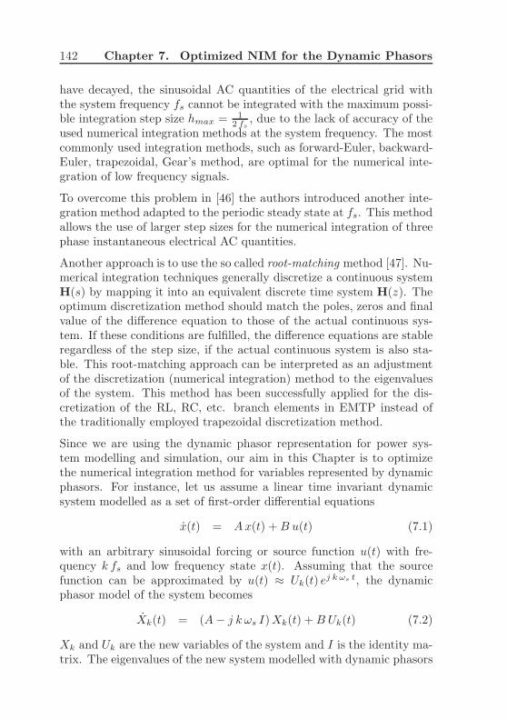
142 Chapter 7. Optimized NIM for the Dynamic Phasors
have decayed, the sinusoidal AC quantities of the electrical grid withthe system frequency fs cannot be integrated with the maximum possi-ble integration step size hmax = 1
2 fs, due to the lack of accuracy of the
used numerical integration methods at the system frequency. The mostcommonly used integration methods, such as forward-Euler, backward-Euler, trapezoidal, Gear’s method, are optimal for the numerical inte-gration of low frequency signals.
To overcome this problem in [46] the authors introduced another inte-gration method adapted to the periodic steady state at fs. This methodallows the use of larger step sizes for the numerical integration of threephase instantaneous electrical AC quantities.
Another approach is to use the so called root-matching method [47]. Nu-merical integration techniques generally discretize a continuous systemH(s) by mapping it into an equivalent discrete time system H(z). Theoptimum discretization method should match the poles, zeros and finalvalue of the difference equation to those of the actual continuous sys-tem. If these conditions are fulfilled, the difference equations are stableregardless of the step size, if the actual continuous system is also sta-ble. This root-matching approach can be interpreted as an adjustmentof the discretization (numerical integration) method to the eigenvaluesof the system. This method has been successfully applied for the dis-cretization of the RL, RC, etc. branch elements in EMTP instead ofthe traditionally employed trapezoidal discretization method.
Since we are using the dynamic phasor representation for power sys-tem modelling and simulation, our aim in this Chapter is to optimizethe numerical integration method for variables represented by dynamicphasors. For instance, let us assume a linear time invariant dynamicsystem modelled as a set of first-order differential equations
x(t) = Ax(t) +B u(t) (7.1)
with an arbitrary sinusoidal forcing or source function u(t) with fre-quency k fs and low frequency state x(t). Assuming that the sourcefunction can be approximated by u(t) ≈ Uk(t) e
j k ωs t, the dynamicphasor model of the system becomes
Xk(t) = (A− j k ωs I)Xk(t) +B Uk(t) (7.2)
Xk and Uk are the new variables of the system and I is the identity ma-trix. The eigenvalues of the new system modelled with dynamic phasors

7.2. Linear Multi-step Methods 143
are shifted by −j k ωs. This frequency shift gives rise to faster oscilla-tions in the step response, which decay in stable systems, depending onthe real part of the eigenvalues. These fast oscillations are inherent todynamic phasor models. As mentioned previously, in the root match-ing method, the poles, zeros and final value of the discrete time systemare matched to those of the actual continuous system. The idea nowis to relax this condition of root-matching and to match the numericalintegration not exactly to the eigenvalues of the dynamic phasors butapproximately to the oscillatory frequencies k ωs of the dynamic phasorsXk.
The Chapter is organized as follows. First a general overview of thenumerical integration techniques will be given with the major focus onthe linear multi-step methods. This is followed by the investigation ofthe numerical integration techniques in the frequency domain, which al-lows us to derive the desired frequency matched discretization methods.The accuracy and efficiency of these derived methods will be comparedwith the traditional numerical integration methods in a simple powersystems example modelled with dynamic phasors.
7.2 Linear Multi-step Methods
Numerical integration techniques generally discretize a continuous sys-tem H(s) by mapping it into an equivalent discrete time system H(z)by using the discretization function (2.11) Ψ. For example a first ordernonlinear ordinary differential equation of the form
x(t) = f(x, t)
is mapped into a discrete time system by using a discretization functiongenerally given as
xn+1 = Ψ (hn+1, [xn, xn−1, ..], [f(xn+1), f(xn), ..])
The discretization function uses the previously computed values of thestate variables and their derivatives to compute approximately the cur-rent value of the state variables. An integration method defined inequation (2.11) must satisfy certain criteria concerning:
• Numerical Accuracy

144 Chapter 7. Optimized NIM for the Dynamic Phasors
• Numerical Stability
• Numerical Efficiency
Numerical Accuracy: An integration method approximates the value atx(tn+1) by the given function Ψ in equation (2.11). The error producedat each step can be defined as |x(tn+1) − xn+1|, under the assumptionthat the numerical solution xn at tn coincides with the real solutionx(tn). This error introduced by advancing the solution from tn to tn+1
in a single step is called also the local truncation error εl. Numericalaccuracy ensures that this error remains bounded during the simulation.Especially for the stationary solution the local truncation error shouldbecome zero.
Numerical Stability: The local error εl incurred at each step should notpropagate to future times. Otherwise the error would increase and thenumerical solution would diverge.
Numerical Efficiency: Major points influencing efficiency of an numer-ical integration algorithm are:
• Number of computational operations in function Ψ at each step.
• Number of executions of Ψ during the simulation, which mainlydepends on the used step size h.
• Memory needed to store the precalculated values needed for theevaluation of Ψ.
After outlining some important criteria for practical numerical integra-tion methods, we will focus on an important class of these methods,namely the linear multi-step methods. The most commonly employednumerical integration techniques such as the forward-Euler, backward-Euler, trapezoidal rule, Gear’s method belong to this family of numeri-cal integration methods [24]. A linear multi-step method’s discretizationfunction Ψ is a linear combination of previously computed values of thestate variables x and their derivatives x.
A multi-step integration method of degree p has the form:
x(tn+1) ≈p∑
i=0
ai x(tn − i h) +
p∑
i=−1
bi x(tn − i h) (7.3)

7.2. Linear Multi-step Methods 145
Methods with b−1 = 0 are called explicit methods, and methods withb−1 6= 0 are called implicit methods. Several methods can be derivedby pre-defining some of the coefficients in (7.3). For example by settinga1 = a2 = a3 = .....ap = 0, we will get Adam’s Methods.
• Adam’s Bashforth Methods (b−1 = 0, p = k − 1)
xn+1 = a0 xn +
p∑
i=0
bi f(xn−i)
• Adam’s Moulton Methods (b−1 6= 0, p = k − 2)
xn+1 = a0 xn +
p∑
i=−1
bi f(xn−i)
where k is defined as the order of the numerical integration method.Adam’s Moulton Methods are implicit methods and therefore they haveto be solved iteratively at every integration step. Iterative methods gen-erally require an initial guess for the solution of nonlinear equations. Agood initial guess reduces the number of required iterations for conver-gence which directly affects the computational efficiency of the method.Such an initial guess e.g. can be calculated by an explicit Adam’s Bash-forth method of the same order.
xpn+1 = a0,p xn + b0,p f(xn) + b1,p f(xn−1) (7.4)
with the coefficients a0,p = 1, b0,p = 32 and b1,p = − 1
2 . This pro-cess is often referred to as a predictor-corrector approach, since Adam’sBashforth method predicts the solution and Adam’s Moulton methodcorrects the solution. The predictor-corrector approach is commonlyemployed in conjunction with local truncation error estimation, whichis then used for an adaptive step-size selection. If a predictor-correctorapproach with same orders k is used the local truncation error can beapproximated as εl(t) = C |xp − x|, with xp the predictor, x the correc-tor solution and C a constant dependent on the order of used method.
Our focus in this section will be on the most frequently used 2nd orderAdam’s Moulton method, known also as trapezoidal method, on whichwe will base our new frequency matched methods. The trapezoidalmethod is also commonly used in the simulation of electromagnetic tran-sients [4]. As our aim is to derive a method which is matched to the

146 Chapter 7. Optimized NIM for the Dynamic Phasors
oscillatory frequencies kωs of the dynamic phasors Xk, it is convenientto investigate the numerical integration techniques in the frequency do-main.
In the case of 2nd order Adam’s Moulton method the time domainapproximation of x(t+ h) is given by the following general expression.
x(t+ h) ≈ a0 x(t) + b−1 x(t+ h) + b0 x(t) (7.5)
or in discrete form
xn+1 = a0 xn + b−1 f(xn+1) + b0 f(xn) (7.6)
In the case of the trapezoidal method the coefficients are a0 = 1 andb0 = b−1 = h
2 . In the following we want to focus on the error analysis inthe frequency domain and numerical stability of the trapezoidal method.
7.2.1 Error Analysis in Frequency Domain
The generalized local truncation error of the 2nd order Adam’s Moultonmethod is given as
εl(t+ h) = x(t+ h) − [a0 x(t) + b−1 x(t+ h) + b0 x(t)] (7.7)
The Laplace transformation of the local truncation error yields
Σl(s)=X(s)(es h − a0 − b−1se
s h − b0s)
︸ ︷︷ ︸
El(s)
(7.8)
Generally the numerical integration methods are optimized for DC sta-tionary solutions meaning that the local truncation error becomes zeroat s = 0 (El(0) = 0). This is also observable in Figure 7.1, which de-picts the frequency response of the local error function El(s) for thetrapezoidal method. The derivation of the trapezoidal method can alsobe accomplished in the frequency domain. The coefficients a0, b−1 andb0 in the general formulation of the 2nd order Adam’s Moulton can alsobe determined from the local error function in the frequency domainEl(s) in such a way, so that the local error function El(s) has a tripleroot at DC (s = 0). This leads to the solution of the following three

7.2. Linear Multi-step Methods 147
f [Hz]
|El(j
ω)|
h = 0.001h = 0.002
-100 -50 0 50 1000
0.01
0.02
0.03
0.04
0.05
Figure 7.1: Error frequency response El(s) of Trapezoidal Method
equations with three unknown coefficients a0, b−1 and b0
El(0) = 1 − a0 = 0 (7.9)
dEl(0)
ds= h− b−1 − b0 = 0 (7.10)
d2El(0)
ds2= h2 − 2 b−1 h = 0 (7.11)
The solution yields the well known coefficients of the trapezoidal methodnamely a0 = 1, b−1 = h
2 and b0 = h2 . Such an investigation of the
local truncation error in the frequency domain opens new possibilitiesto derive new numerical integration methods which are not optimizedat DC but at also other frequencies.
7.2.2 Numerical Stability Analysis
Numerical Stability is one of the most important properties of the nu-merical integration methods. Numerical stability ensures that the localtruncation error remains bounded in subsequent integration steps. Thestandard method for testing numerical stability is to investigate how theeigenvalues of the continuous time system (s) are mapped to the eigen-values of the discrete time system (z). Numerical stable methods mapthe stable eigenvalues of the continuous time system with ℜ{s} < 0to eigenvalues in discrete time system with |z| < 1. For the 2nd orderAdam’s Moulton method, this can be calculated by replacing z = es h

148 Chapter 7. Optimized NIM for the Dynamic Phasors
in (7.8) and solving El(s) = 0 in z yielding
z =a0 + b0 s
1 − b−1 s
Thus, the stability condition becomes
|z| =
∣∣∣∣
a0 + b0 s
1 − b−1 s
∣∣∣∣< 1 (7.12)
In case of the trapezoidal method with pure real coefficients and s =σ + j ω the stability condition yields
(a0 + b0 s) (a0 + b0 s)∗ < (1 − b−1 s) (1 − b−1 s)
∗
1 +h2
4|s|2 + hℜ{s} < 1 +
h2
4|s|2 − hℜ{s}
ℜ {s} < 0
σ < 0
This means, that stable continuous time systems with ℜ{s} < 0 aremapped directly to stable discrete time systems with |z| < 1 regardlessof the selected step size h. Such numerical integration methods mappingstable continuous time systems to stable discrete time systems are calledabsolute stable methods or A-stable methods. Figure 7.2 shows |z| asa function of step size h and ℜ{s}. We also observe that 0 < |z| < 1,which is the condition for numerical stability. After the local truncationerror analysis in the frequency domain and the stability region analysisof the trapezoidal method, the focus in the following sections will beon the frequency matched methods and their error and stability regionanalysis.
7.3 Frequency Matched Trapezoidal
Method for Real Signals
If the trapezoidal method is used for the numerical integration of sinu-soidal electrical AC quantities with system frequency (e.g. 50 Hz), theycannot be integrated with the maximum possible integration step sizedue to the lack of accuracy of the trapezoidal methods at the systemfrequency. As Figure 7.1 shows, the local truncation of the trapezoidal

7.3. Frequency Matched TR-Method for Real Signals 149
h
σ
|z|
00.02
0.040.06
0.08
-100
-50
00
0.5
1
1.5
2
Figure 7.2: Region of Stability (|z| < 1) of the Trapezoidal Method as afunction of the step size h and the real part of the eigenvalueσ = ℜ{s}
method at 50 Hz is much higher than at DC frequencies, so that the stepsize must be kept small enough to achieve the same degree of accuracyat 50 Hz.
To overcome this problem, in [46] the authors propose the use of a newnumerical integration method which is adapted to the periodic steadystate of the electrical AC quantities. With this method, it is possibleto compute the sinusoidal AC state variables with angular frequency ωsat steady state exactly without introducing a local truncation error re-gardless of the selected step size h. This is achieved by investigating thelocal truncation error εl(t) in the frequency domain. The investigationof the local error function in the frequency domain opens new possi-bilities to derive new numerical integration methods yielding minimumlocal truncation error not only at DC but also at other frequencies.The coefficients a0, b−1 and b0 can be calculated in such a way thatthe roots of El(s) in (7.8) are placed at frequencies other than DC. Asstated in [46], the coefficients a0, b−1 and b0 can be calculated in sucha way that the roots of El(s) are placed at −jωs, 0 and jωs. The newcoefficients a0, b−1 and b0 are determined by solving the the following

150 Chapter 7. Optimized NIM for the Dynamic Phasors
three equations.
El(0) = 1 − a0 = 0 (7.13)
El(j ωs ) = ej ωs h − a0 − jb−1 ωs ej ωs h − jb0 ωs = 0 (7.14)
El(−j ωs ) = e−j ωs h − a0 + jb−1 ωs e−j ωs h + jb0 ωs = 0 (7.15)
The solution of (7.13-7.15) yields
a0 = 1 (7.16)
b0 =j
ωs
1 − ej ωs h
1 + ej ωs h=
1
ωstan
(ωs h
2
)
(7.17)
b−1 =1
ωstan
(ωs h
2
)
(7.18)
With equation (7.6) and the new coefficients a0, b−1 and b0 the fre-quency matched trapezoidal method is fully defined. In the following,a local truncation error analysis will be performed on the new methodin the frequency domain.
7.3.1 Error Analysis in Frequency Domain
Figure 7.3 shows the frequency response of the local truncation errorfor the frequency matched trapezoidal method for real variables at ωs =2 π 50 s−1 for different step sizes h. The desired frequency response of
f [Hz]
|El(j
ω)|
h = 0.001h = 0.002
-100 -50 0 50 1000
0.01
0.02
0.03
0.04
0.05
Figure 7.3: Error frequency response El(s) of Matched Trapezoidal forreal variables
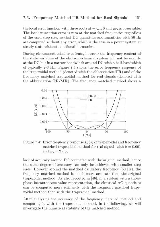
7.3. Frequency Matched TR-Method for Real Signals 151
the local error function with three roots at −jωs, 0 and jωs is observable.The local truncation error is zero at the matched frequencies regardlessof the used step size, so that DC quantities and quantities with 50 Hzare computed without any error, which is the case in a power system atsteady state without additional harmonics.
During electromechanical transients, however the frequency content ofthe state variables of the electromechanical system will not be exactlyat the DC but in a narrow bandwidth around DC with a half-bandwidthof typically 2-3 Hz. Figure 7.4 shows the error frequency response ofthe trapezoidal method (denoted with the abbreviation TR) and of thefrequency matched trapezoidal method for real signals (denoted withthe abbreviation TR-MR). The frequency matched method shows a
f [Hz]
|El(j
ω)|
TR-MRTR
-100 -50 0 50 1000
0.002
0.004
0.006
0.008
0.01
Figure 7.4: Error frequency response El(s) of trapezoidal and frequencymatched trapezoidal method for real signals with h = 0.001and ωs = 2 π 50
lack of accuracy around DC compared with the original method, hencethe same degree of accuracy can only be achieved with smaller stepsizes. However around the matched oscillatory frequency (50 Hz), thefrequency matched method is much more accurate than the originaltrapezoidal method. As also reported in [46], in a system with a three-phase instantaneous value representation, the electrical AC quantitiescan be computed more efficiently with the frequency matched trape-zoidal method than with the trapezoidal method.
After analyzing the accuracy of the frequency matched method andcomparing it with the trapezoidal method, in the following, we willinvestigate the numerical stability of the matched method.

152 Chapter 7. Optimized NIM for the Dynamic Phasors
7.3.2 Numerical Stability Analysis
As discussed in Section 7.2.2, the general condition for numerical sta-bility of the 2nd order Adam’s Moulton method is given in (7.12). Inthe case of the frequency matched trapezoidal method, the coefficientsare also real valued. Thus the stability condition becomes
(a0 + b0 s) (a0 + b0 s)∗ < (1 − b−1 s) (1 − b−1 s)
∗
a20 + b20 |s|2 + 2 b0 ℜ{s} < a2
0 + b−1 |s|2 − 2 b−1 ℜ{s}b0 ℜ{s} < 0
b0 σ < 0
For stable systems (σ < 0) the condition for numerical stability becomes
b0 > 0
1
ωstan
(ωs h
2
)
> 0
k π <ωs h
2< (2 k + 1)
π
2k
fs< h <
2 k + 1
2 fs(7.19)
with k ∈ N. The expression for k = 0, namely h < 12 fs
, reflects theNyquist sampling theorem.
Figure 7.5 depicts |z| as a function of step size h and ℜ{s}. In contrastto the trapezoidal method, the stability range of the frequency matchedtrapezoidal method for real signals is limited. We observe that |z| < 1is only valid for step sizes (h) fulfilling the condition 7.19. However, thestep size can be increased till hmax = 1
2 fsas dictated by the Nyquist
criterion. If the used step size is outside of the valid stability region(e.g. 1
2 fs< h < 1
fs), the stable continuous system is mapped to an
instable discrete time system. Thus the matched trapezoidal methodfor real signals is not an A-stable method.
The described method has been successfully employed for the simulationof power system transients represented with three-phase instantaneousvalues, where the steady state is described by the periodic AC quantities[46]. The same method can also be applied to systems represented bydynamic phasors. In contrast to the three-phase instantaneous values,the dynamic phasor quantities are constant at steady state. Thus, the

7.3. Frequency Matched TR-Method for Real Signals 153
h
σ
|z|
00.02
0.040.06
0.08
-100
-50
00
0.5
1
1.5
2
Figure 7.5: Region of Stability (|z| < 1) of the Trapezoidal Methodmatched at −jωs, 0 and jωs as a function of the step size hand the real part of the eigenvalue σ = ℜ{s}
traditional trapezoidal method (and also other linear multi step meth-ods such as backward Euler or Gear’s Method) can be used for thenumerical integration of dynamic phasor quantities. The dynamic pha-sor representation is a baseband representation so that DC optimized(matched) numerical integration methods are accurate enough after fasttransients have decayed. However as discussed previously, during fasttransients with high frequencies, the trapezoidal method gets inaccurateand inefficient. The main idea of using such a frequency matched nu-merical integration is to increase the simulation accuracy and efficiencyduring the fast transients inherent to the dynamic phasors approachdue to the shift of the eigenvalue’s oscillatory frequency as mentionedin Section 7.1.
The decreased accuracy of the frequency matched method around DCis not that critical, if it is used in conjunction with three-phase instan-taneous values, as they are not DC at steady state but rather periodicwith system frequency fs. However, the use of the frequency matchedmethod in conjunction with dynamic phasors requires a high accuracyaround oscillatory frequencies k ωs and DC.

154 Chapter 7. Optimized NIM for the Dynamic Phasors
In the following Section, we will derive another frequency matchedmethod based again on the trapezoidal method, which is more accu-rate and numerically A-stable.
7.4 Frequency Matched Trapezoidal
Method for Complex Signals
In the previous Section, a method was derived, which is optimized forthe numerical integration of real sinusoidal signals with frequency fs orfrequencies around fs. However as discussed in Section 3.3, real band-pass signals can also be represented by their analytical counterparts,as they contain all the information about the original bandpass signal.The major advantage of using an analytical or complex signal is thatthe bandwidth of the original signal is reduced, as only positive (ornegative) frequency components of the real signal are considered.
The frequency matched trapezoidal method described in the previousSection was derived for the numerical integration of periodic real band-pass signals. In this case the derivation of the frequency matched trape-zoidal method was performed by placing two of the three roots of thelocal error in frequency domain at −j ωs and j ωs as real valued sinu-soidal signals’ spectra with angular frequency ωs are located at thesefrequencies. The representation of the real bandpass signals by theiranalytical counterparts brings one additional freedom in the placing ofthe roots, as the complex signal has only frequency component at posi-tive or negative frequency. Hence, only one root has to be placed at thefrequency j ωs or −j ωs, the remaining two roots can be placed at DC.
In the following, the new method will be derived by using the samemethodology as in previous sections, namely calculation of the coeffi-cients a0, b−1 and b0 in such a way that the two roots of El(s) in (7.8)are placed at DC and one at j ωs. The new coefficients a0, b−1 and b0are determined by solving the the following three equations.
El(0) = 1 − a0 = 0 (7.20)
dEl(0)
ds= h− b−1 − b0 = 0 (7.21)
El(j ωs ) = ej ωs h − a0 − j ωs ej ωs h b−1 − j ωs b0 = 0 (7.22)

7.4. Frequency Matched TR-Method for Complex Signals155
The solution of (7.20-7.22) yields
a0 = 1 (7.23)
b0 =h
2+ j
(1
ωs− h
2cot
(ωs h
2
))
(7.24)
b−1 =h
2− j
(1
ωs− h
2cot
(ωs h
2
))
(7.25)
As a next step, an error analysis will be performed on the new frequencymatched method and will be compared with to antecedently discussedmethods.
7.4.1 Error Analysis in Frequency Domain
Figure 7.6 pictures the frequency response of the local truncation errorfor the frequency matched trapezoidal method for complex variables atωs = 2 π 50 s−1 for different step sizes h. The desired frequency re-
f [Hz]
|El(j
ω)|
h = 0.001h = 0.002
-100 -50 0 50 1000
0.01
0.02
0.03
0.04
0.05
Figure 7.6: Error frequency response El(s) of Matched Trapezoidal forcomplex variables
sponse of the local error function with three roots double root at DCand a single root j ωs is viewable. The local truncation error is zeroat the matched frequencies regardless of the used step size, so that DCquantities and complex periodic quantities with 50 Hz are computedwithout any error. Figure 7.7 shows the error frequency response of thetrapezoidal method (denoted with the abbreviation TR), the frequency

156 Chapter 7. Optimized NIM for the Dynamic Phasors
matched trapezoidal method for real signals (denoted with the abbre-viation TR-MR) and the frequency matched trapezoidal method forcomplex signals (denoted with the abbreviation TR-MC). As expected,
f [Hz]
|El(j
ω)|
TR-MRTR-MCTR
-100 -50 0 50 1000
0.002
0.004
0.006
0.008
0.01
Figure 7.7: Error frequency response El(s) of trapezoidal, frequencymatched trapezoidal methods for real and complex variableswith h = 0.001 and ωs = 2 π 50
placing two roots at DC in the error frequency response El(s) increasedthe accuracy of the method for complex signals compared to the onefor real signals. The frequency matched method for complex signals ismore accurate than the matched method for real signals around DC andalso around j ωs.
Used in conjunction with predictor-corrector approach, the coefficientsof the explicit predictor method (7.4) can be determined in the sameway by placing two roots at DC and one root at j ωs yielding
a0,p=1
b0,p=h
2+
sin (ωsh)
ωs+ j
(h
2
(sin (ωsh)
1 − cos (ωsh)
)
− cos (ωsh)
ωs
)
b1,p=h
2− sin (ωsh)
ωs+ j
(cos (ωsh)
ωs− h
2
(sin (ωsh)
1 − cos (ωsh)
))
7.4.2 Numerical Stability Analysis
Same procedures as in previous sections will be applied to define theregion of stability of the new method. In the case of the frequency

7.4. Frequency Matched TR-Method for Complex Signals157
matched trapezoidal method, the coefficients b0 and b−1 are complexvalued but are also conjugate complex, meaning b−1 = b∗0. With (7.23-7.25), the stability condition becomes
(a0 + b0 s) (a0 + b0 s)∗
< (1 − b−1 s) (1 − b−1 s)∗
a20 + |b0 s|2 + 2ℜ{b0 s} < a2
0 + |b−1 s|2 − 2ℜ{b−1 s}ℜ {b0 s} < −ℜ{b∗0 s}
σ < 0
As in the case of trapezoidal method, this method is also an A-stablemethod mapping stable continuous time systems (ℜ{s} < 0) directlyto stable discrete time systems (|z| < 1) irrespective of the selected stepsize h. Figure 7.8 depicts |z| for the new method as a function of stepsize h and ℜ{s}.
h
σ
|z|
00.02
0.040.06
0.08
-100
-50
00
0.5
1
1.5
2
Figure 7.8: Region of Stability (|z| < 1) of the Trapezoidal Methodmatched at 0, 0 and jωs as a function of the step size h andthe real part of the eigenvalue σ = ℜ{s}
The described frequency matched method for complex signal is numeri-cally stable and has also higher DC accuracy compared with the one forreal signals. Thus, it can also be used in conjunction with the dynamicphasors.

158 Chapter 7. Optimized NIM for the Dynamic Phasors
In the next section, the accuracy and efficiency of these derived fre-quency matched methods will be compared to the traditional trape-zoidal method in two simple examples.
7.5 Test Cases
In the previous sections the focus was on the derivation of the frequencymatched methods. The aim of this section is to compare the accuracyand efficiency of these methods with each other and verify the previouslymade conclusions by simulations. In this section, the derived numericalintegration methods will be used for the simulation of two test sys-tems. As a first example, a system of ordinary differential equationswith known analytic solution will be solved numerically by using thediscussed numerical integration methods. Second example is the SingleMachine Infinite Bus system, which has been also used in Section 4.4.
All three methods use a variable step-size selection algorithm based onthe described local truncation error estimation with predictor-correctorapproach. Simulations were obtained using Matlab 7.1 running on aIntel Pentium IV CPU with 3.80 GHz and 2 GB of RAM.
7.5.1 Example with Analytic Solution
In this case study, the traditional trapezoidal method, frequency match-ed trapezoidal methods for real signals and for complex signal will beused for the numerical integration of a 4th order ordinary differentialequation system, whose analytic solution is also known. The resultsof the three integration methods will be compared regarding accuracyand computational efficiency. The differential equation system underconsideration is given as
x1 = −σ1 x1 − ω1 x2
x2 = −σ1 x2 + ω1 x1
x3 = −σ2 x3 − ω2 x4
x4 = −σ2 x4 + ω2 x3
y1 = x1 + x3
y2 = x2 + x4

7.5. Test Cases 159
with the parameter ω1 = 2 π 3, ω2 = 2 π 60, σ1 = 3, σ2 = 6 and theinitial values x1(0) = 1, x2(0) = 0, x3(0) = 1, x4(0) = 0. The analyticsolution of the initial value problem yields
x1 = cos(ω1 t) e−σ1 t
x2 = sin(ω1 t) e−σ1 t
x3 = cos(ω2 t) e−σ2 t
x4 = sin(ω2 t) e−σ2 t
The system is integrated using the TR, TR-MR (matched at −j ω2, 0and j ω2) and TR-MC (matched at 02 and −j ω2). Figure 7.9 shows theresults of the analytic solution and the numerical solution computedwith three methods discussed in previous sections in the overall simu-lation interval 0 < t < 1.4 and in a zoomed section with the requiredCPU simulation times. In the zoomed section we observe that the TRmethod has lack of accuracy during high frequency oscillations withω2 = 2 π 60, where the frequency matched methods (TR-MR,TR-MC)give almost the accurate results during this fast transients. But if thefast transients have decayed and the system behavior is governed by lowfrequency transients with ω1 = 2 π 3, TR-MR method has less accurateresults. However, the TR-MC method computes the results with highdegree of accuracy during fast and slow transients. Comparison of theoverall CPU simulation times of all three integration methods showsthat the TR-MC is also the fastest method for this simple test case.
7.5.2 SMIB system
The Single Machine Infinite Bus (SMIB) system will be simulated as asimple power system example modelled dynamic phasors approach. Thecomponents of the system are modelled by dynamic phasors and are rep-resented in the original three phases (ABC). Same test case has been alsoused in Section 4.4 for the simulation of unbalanced and asymmetricalconditions with dynamic phasors. The simulated system has overall 40differential and 150 algebraic variables. In this test case, a single-phaseto ground fault occurs at the BUS2 end of the LINE3 at 0.1 secondsand is removed after 0.20 seconds by disconnecting the line. It is im-portant to mention, that the approximating set of Fourier coefficients isselected as K = {1} for the transmission line model and K = {0, 1, 2}for the synchronous machine model, as unbalanced conditions are of

160 Chapter 7. Optimized NIM for the Dynamic Phasors
Time [s]
y1
Analytic
TR
TR-MR
TR-MC
Time [s]
y1
Analytic
TR
TR-MR
TR-MC
0.21 0.215 0.22 0.225
0 0.2 0.4 0.6 0.8 1 1.2
-0.6
-0.4
-0.2
0
-1
0
1
2
Figure 7.9: Analytic solution of y1 compared with numerical solutioncalculated with the three different integration methods andrequired CPU simulation times
concern. The dynamic behavior of the test case is simulated by usingthe trapezoidal method and frequency matched trapezoidal methods forreal and complex signals by using the same degree of accuracy for thethree methods (error tolerance 10−3).
First simulation is done by using the traditional trapezoidal method(TR) for all dynamic phasorsXk. In the second simulation, the dynamicphasors with k = 0 are discretized using TR and with k > 0 using TR-MR with the frequencies matched to −j k ωs, 0 and j k ωs. In the thirdsimulation, the dynamic phasors with k = 0 are discretized using TRand with k > 0 using TR-MC with the frequencies matched to −j k ωsand 02 (with double root at 0).

7.5. Test Cases 161
Time [s]
〈Te〉 0
[pu]
DT
TR
TR-MR
TR-MC
Time [s]
〈Te〉 0
[pu]
DT
TR
TR-MR
TR-MC
0.24 0.26 0.28 0.3 0.32 0.34 0.36
0 0.5 1 1.5 2 2.5
0.2
0.4
0.6
0.8
1
1.2
0
0.5
1
1.5
DT TR TR-MR TR-MC
186.125 [s] 25.410 [s] 49.750 [s] 26.045 [s]
Figure 7.10: Evolution of the positive sequence electrical torque Te,0computed with TR, TR-MR and TR-MC (all with εtol =10−3) compared with the detailed simulation (TR withεtol = 10−6) and required CPU simulation times
Figure 7.10 shows the evolution of the positive sequence electrical torqueTe,0 computed with TR, TR-MR and TR-MC compared with the de-tailed simulation (DT), which is computed with TR method by keepingthe error tolerance quite low (10−6), which ensures an accurate simula-tion. The table in Figure 7.10 shows also the required CPU simulationtimes with different integration methods.
In the zoomed section in Figure 7.10 with fast transients around ωs, thehigher accuracy of the TR-MR and TR-MC methods compared with TR

162 Chapter 7. Optimized NIM for the Dynamic Phasors
method is observable, where the TR-MR and TR-MC methods are inoverall agreement with the detailed simulation results. The increasedaccuracy and efficiency of the TR-MC method at DC ( also at ωs)becomes noticeable in the comparison of the overall CPU simulationtimes. TR-MC method is two times faster than the TR-MR methoddue to its increased accuracy also for DC frequencies and as fast as theTR method in this test case.

7.6. Summary 163
7.6 Summary
In this Chapter, a numerical integration method based on the trape-zoidal method is derived for the simulation of systems modelled withdynamic phasors by minimizing the local truncation error around theoscillatory frequency (kωs) of the dynamic phasors (Xk). This wasachieved by investigating the local truncation error of the trapezoidalmethod in the frequency domain and placing the roots of the error func-tion at the desired matched frequencies −j k ωs, 0 and j k ωs so that thereal sinusoidal signals at k ωs can be computed without any error re-gardless of the selected step size. The use of complex/analytic signalrepresentation facilitated the improvement of the numerical accuracy,efficiency and stability of the derived method by placing a double rootat 0 and only one root at j k ωs or −j k ωs compared with frequencymatched methods used for real signals.
The frequency matched method shows a better performance regard-ing accuracy and efficiency during fast transients with the frequenciesaround kωs than the trapezoidal method. During slow transients withlow frequencies, the frequency matched trapezoidal method for complexsignals is computationally more efficient the trapezoidal method for realsignals, due to its decreased error around DC. Besides its accuracy andefficiency, another important property of the frequency matched methodfor complex signals is its numerical A-stability, where the frequencymatched method for real signals does not have this property.


Chapter 8
Conclusions and Outlook
In this thesis, a new simulation tool has been developed and imple-mented which enables the combined simulation of the electromagneticand electromechanical transients by using the dynamic phasor repre-sentation of the power system and its components. The main ideabehind the dynamic phasors approach is to represent the system quan-tities by their time varying Fourier coefficients. The system quanti-ties have generally a bandpass characteristic with their frequency con-tents centered around the system frequency or multiples of the sys-tem frequency, whereas the time varying Fourier coefficients are base-band/lowpass quantities around DC. Thus the frequency content of thesimulated quantities is decreased, which allows the use of larger stepsizes during simulation process and thus increases the simulation speed.
For this purpose, a systematic and general simulation framework basedon the Differential Switched Algebraic State-Reset (DSAR) representa-tion of hybrid systems, has been developed facilitating a modular andflexible model development. Based on this general simulation frame-work, the dynamic phasor models of major power system components,e.g. synchronous machines, doubly-fed induction generator (DFIG),thyristor-controlled series capacitor (TCSC), etc. have been developedand implemented with the new simulation tool. With the dynamic pha-sors approach, besides the fundamental frequency component also otherharmonics can be included in the model derivation. Such harmonics oc-cur for example in the TCSC model equations due to the periodicalswitchings of the thyristors or also in the electrical machine equations
165

166 Chapter 8. Conclusions and Outlook
in the DQ0 reference frame due to the negative and zero sequence com-ponents during unbalanced conditions. The simulation performance ofthese models regarding accuracy and efficiency has been compared sys-tematically to that traditionally achieved with electromagnetic tran-sients programs. Simulations have shown that the dynamic phasormodels have nearly the same degree of accuracy compared with thedetailed time-domain models if appropriate approximations are madein the model derivation. In terms of computational speed, the dynamicphasor models proved to be more efficient than the detailed time-domainmodels. Simulations with dynamic phasors were 5-10 time faster thanwith the detailed time domain models, by maintaining a high degree ofaccuracy.
The systematic derivation and formulation of the dynamic phasor ap-proach based on their original detailed time-domain models allow alsosome model simplification depending on the nature of study. In this way,reduced order dynamic phasor models have been derived which are in away equivalent to the fundamental frequency models used in transientstability programs neglecting the fast network-side fast electromagnetictransients. With such reduced order dynamic phasor models it waspossible also to include other harmonics in the model derivation like inthe detailed dynamic phasor models but neglect their fast electromag-netic transients. With this systematic and appropriate order reduction,we were able to simulate unbalanced conditions even with fundamentalfrequency equivalent models efficiently.
Numerical integration techniques and algorithms play a significant rolein the simulation of dynamical systems such as power systems. There-fore efforts also have been made on the derivation of methods suitable forthe numerical integration of systems represented by dynamic phasors byinvestigating the numerical integration techniques in the frequency do-main. The derived frequency-matched trapezoidal method for complexsignals increased the accuracy and the efficiency of the simulations withsystems represented by dynamic phasors compared with the commonlyused trapezoidal method.
The prototype of the simulation tool has been implemented in MAT-LAB. The basic steps have been taken to implement the developedmodels and algorithms also in the commercial simulation program NE-PLAN [1] for power system analysis. In NEPLAN, the dynamic phasormodels in the ABC reference frame are implemented.

167
Outlook
The main purpose of the thesis was to develop an appropriate prototypeof a new simulation tool for the simulation of power system dynamicswith the dynamic phasor models of the power system components. Nextstep will be to complete the started integration of the developed simu-lation framework and the derived dynamic phasor models in NEPLAN,which is a full commercial software program for power system analysis.
The future work in the scope of this thesis can include the followingsubjects.
• In terms of existing models, the existing library of dynamic phasormodels should be extended by other commonly used power systemcomponents such as other FACTS devices (SVC, HVDC, UPFC,etc.), detailed transformer models etc. In the derived DFIG dy-namic phasor model, our focus was more on the component itselfand not on the complete wind turbine including also the controls(e.g. pitch control) or protections (e.g. crow bar protection). Thederived DFIG model must be augmented by the commonly usedcontrol and protection models.
• As mentioned in Chapter 1, one commonly applied approach tocombine the accuracy of the EMTP and the computational ef-ficiency of the TSP is to model and simulate some parts of thesystem with a detailed full time domain representation (EMTP)and the rest of the system in the quasi-steady state fundamentalfrequency representation (TSP) and interface the different mod-elling approaches appropriately. The drawback of this approachis that only the fundamental frequency components can be inter-faced in this algorithm and other harmonics are omitted. This ideacan be improved by using the dynamic phasor models instead ofthe fundamental frequency models in this approach as also otherharmonics can also be included in the dynamic phasor models.
• In terms of the numerical algorithms optimized for dynamic pha-sors, the combined usage of the here derived frequency matchedtrapezoidal method for complex signals with traditionally usedmethods such as the Trapezoidal, Gear’s method etc. can fur-ther improve the simulation performance. The frequency matched

168 Chapter 8. Conclusions and Outlook
trapezoidal method for complex signals can be employed right af-ter large disturbances in the system and can be used for the nu-merical integration of the fast oscillations inherent to the dynamicphasor models. But if these fast oscillations have decayed onecould switch back to the traditional methods which are optimizedfor the integration of signals with frequencies near to DC.
• In terms of the numerical algorithms of the simulation framework,the general simulation and modelling framework developed hereis based on the fully implicit and nonlinear representation of thesystem and model equations, so that also the overall numericalintegration is based on implicit and iterative methods. Advantagesof linear systems can be incorporated in the simulation process byemploying computationally more efficient methods for the linearpart of the system.

Bibliography
[1] BCP, “NEPLAN - Power System Analysis Tool,http://www.neplan.ch,” 1988-2007.
[2] S. M. Rinaldi, J. P. Peerenboom, and T. K. Kelly, “Identifying,understanding, and analyzing critical infrastructure interdependen-cies,” Control Systems Magazine, IEEE, vol. 21, no. 6, p. 11, 2001.
[3] P. W. Sauer and M. A. Pai, Power System Dynamics and Stability,1st ed. Prentice Hall, 1997.
[4] H. W. Dommel, “Digital computer solution of electromagnetic tran-sients in single-and multiphase networks,” IEEE Transactions onPower Apparatus and Systems, vol. PAS-88, no. 4, p. 388, 1969.
[5] H. Fankhauser, K. Aneros, A.-A. Edris, and S. Torseng, “Advancedsimulation techniques for the analysis of power system dynamics,”Computer Applications in Power, IEEE, vol. 3, no. 4, pp. 31–36,1990.
[6] J. Astic, A. Bihain, and M. Jerosolimski, “The mixed adams-bdfvariable step size algorithm to simulate transient and long termphenomena in power systems,” Power Systems, IEEE Transactionson, vol. 9, no. 2, pp. 929–935, 1994.
[7] STRI, “SIMPOW - Power System Simulation and Analysis Soft-ware, http://www.stri.se.”
[8] U. Linnert, “Neue Differenzenleitwertverfahren zur Simulation dy-namischer Ausgleichsvorgange mit grossen Schrittweiten,” Archivfur Elektrotechnik, vol. 76, pp. 101–110, 1992.
169

170 Bibliography
[9] S. Henschel, “Analysis of electromagnetic und electromechanicalpower system transients with dynamic phasors,” Ph.D. disserta-tion, University of British Colombia, 1999.
[10] V. Venkatasubramanian, “Tools for dynamic analysis of the gen-eral large power system using time-varying phasors,” InternationalJournal of Electrical Power and Energy Systems, vol. 16, no. 6, p.365, 1994.
[11] R. Adapa and J. Reeve, “A new approach to dynamic analysis of acnetworks incorporating detailed modeling of dc systems. ii. appli-cation to interaction of dc and weak ac systems,” Power Delivery,IEEE Transactions on, vol. 3, no. 4, p. 2012, 1988.
[12] J. Reeve and R. Adapa, “A new approach to dynamic analysis ofac networks incorporating detailed modeling of dc systems. i. prin-ciples and implementation,” Power Delivery, IEEE Transactionson, vol. 3, no. 4, p. 2005, 1988.
[13] S. Sanders, J. Noworolski, X. Liu, and G. Verghese, “Generalizedaveraging method for power conversion circuits,” Power Electron-ics, IEEE Transactions on, vol. 6, no. 2, pp. 251–259, 1991.
[14] P. Mattavelli, G. Verghese, and A. Stankovic, “Phasor dynamicsof thyristor-controlled series capacitor systems,” Power Systems,IEEE Transactions on, vol. 12, no. 3, pp. 1259–1267, 1997.
[15] P. C. Stefanov and A. M. Stankovic, “Modeling of upfc operationunder unbalanced conditions with dynamic phasors,” Power Sys-tems, IEEE Transactions on, vol. 17, no. 2, p. 395, 2002.
[16] A. M. Stankovic, P. Mattavelli, V. Caliskan, and G. C. Verghese,“Modeling and analysis of facts devices with dynamic phasors,” inPower Engineering Society Winter Meeting, 2000. IEEE, vol. 2,2000, p. 1440.
[17] A. Stankovic and T. Aydin, “Analysis of asymmetrical faults inpower systems using dynamic phasors,” Power Systems, IEEETransactions on, vol. 15, no. 3, pp. 1062–1068, 2000.
[18] A. Stankovic, B. Lesieutre, and T. Aydin, “Applications of gener-alized averaging to synchronous and induction machines,” in NorthAmerican Power Symposium, Boston, 1996, pp. 277–282.

Bibliography 171
[19] A. Stankovic, S. Sanders, and T. Aydin, “Dynamic phasors in anal-ysis of unbalanced polyphase ac machines,” IEEE Transactions onEnergy Conversion, vol. 17, no. 1, pp. 107–113, 2002.
[20] I. Hiskens and P. Sokolowski, “Systematic modeling and symboli-cally assisted simulation of power systems,” Power Systems, IEEETransactions on, vol. 16, no. 2, pp. 229–234, 2001.
[21] I. Hiskens and M. Pai, “Trajectory sensitivity analysis of hybridsystems,” IEEE Transactions on Circuits and Systems I: Funda-mental Theory and Applications, vol. 47, no. 2, pp. 204–220, 2000.
[22] MathWorks, “MATLAB - the language of technical computing,visiualization, programming, http://www.mathworks.com,” 1984-2007.
[23] Modelica, “Modeling of complex physical systems,http://www.modelica.org/,” 1997-2007.
[24] M. Crow, Computational methods for electric power systems. CRCPress, 2003.
[25] C. Gear, “The simultaneous numerical solution of differential-algebraic equations.” IEEE Trans. Circuit Theory, vol. CT-18,no. 1, pp. 89–95, 1971.
[26] T. Davis, “UMFPACK, set of routines for solving unsymmetricsparse linear systems,” 2002.
[27] T. Park and P. I. Barton, “State event location in differential-algebraic models,” ACM Trans. Model. Comput. Simul., vol. 6,no. 2, pp. 137–165, 1996.
[28] D. J. Hill, “Nonlinear dynamic load models with recovery forvoltage stability studies,” Power Systems, IEEE Transactions on,vol. 8, no. 1, p. 166, 1993.
[29] F. S. Lawrence, W. R. Mark, and A. K. Jacek, “Solving index-1 daes in matlab and simulink,” SIAM Rev., vol. 41, no. 3, pp.538–552, 1999.
[30] J. H. Taylor, “Rigorous handling of state events in matlab,” in Con-trol Applications, 1995., Proceedings of the 4th IEEE Conferenceon, 1995, p. 156.

172 Bibliography
[31] I. Hiskens and M. Pai, “Hybrid systems view of power system mod-elling,” in Circuits and Systems, 2000. Proceedings. ISCAS 2000Geneva. The 2000 IEEE International Symposium on, vol. 2, 2000,pp. 228–231 vol.2.
[32] Plexim, “PLECS user manual - high-speed simulations of elec-trical and power electronic circuits under matlab/simulink,http://www.plexim.com,” 2007.
[33] P. Kundur, N. J. Balu, and M. G. Lauby, Power system stabilityand control, ser. The EPRI power system engineering series. NewYork: McGraw-Hill, 1994.
[34] S. Haykin, Communication Systems, 2nd ed. New York: Wiley,1983.
[35] R. Z. Muljadi, N. Miller, A. Ellis, and E., “Making connections:Wind generation challenges and progress,” IEEE Power & EnergyMagazine, no. November-December, pp. 26–37, 2005.
[36] P. B. Eriksen, T. Ackerman, H. Abildgaard, P. Smith, and W. Win-ter, “System operation with high wind penetration: The challengesof denmark, germany, spain, and ireland,” IEEE Power & EnergyMagazine, pp. 65–74, 2005.
[37] EWEA, “Wind force 12-a. blueprint to achive 12% of the world’selectricity from wind power by 2020,” European Wind Energy As-sociation, www.ewea.org, Tech. Rep., 2005.
[38] T. Lund, J. Eek, S. Uski, and A. Perdana, “Fault simulation ofwind turbines using commercial simulation tools,” in Proc. FifthInternational Workshop on Large-Scale Integration of Wind Powerand Transmission Networks for Offshore Wind Farms, Glasgow,2005.
[39] J. G. Slootweg, S. W. d. Haan, H. Polinder, and W. L. Kling,“General model for representing variable speed wind turbines inpower system dynamics simulations,” IEEE Transactions on PowerSystems, vol. 18, no. 1, pp. 144–151, 2003.
[40] J. G. Slootweg, H. Polinder, and W. L. Kling, “Representing windturbine electrical generating systems in fundamental frequency sim-ulations,” IEEE Transactions on Power Systems, vol. 20, no. 3, pp.1199–1206, 2005.

Bibliography 173
[41] R. Cano-MarIn, A. Gomez-Exposito, and M. Burgos-Payan, “Windenergy integration in distribution networks: A voltage-stabilityconstrained case study,” in Proceedings of the VI Bulk Power Sys-tem Dynamics and Control, Cortina d’Ampezzo, Italy, 2004.
[42] N. Mohan, T. M. Undeland, and W. P. Robbins, Power Electron-ics:Converters, Applications, and Design. New York: John Wileyand SonsEdition, 1995.
[43] N. G. Hingorani and L. Gyugyi, Understanding FACTS conceptsand technology of flexible AC transmission systems. New York:IEEE Press, 2000.
[44] Y.-H. Song, Flexible ac transmission systems (FACTS). London:The Institution of Electrical Engineers, 1999.
[45] H. A. Othman and L. Angquist, “Analytical modeling of thyristor-controlled series capacitors for ssr studies,” Power Systems, IEEETransactions on, vol. 11, no. 1, p. 119, 1996.
[46] M. Poeller and M. Schmieg, “Exploting multiple time scale prop-erties for fast simulation algorithms,” in Proceedings of the 13thPower Systems Computation Conference, Trondheim, 1999.
[47] N. R. Watson and G. D. Irwin, “Electromagnetic transient simu-lation of power systems using root-matching techniques,” Gener-ation, Transmission and Distribution, IEE Proceedings-, vol. 145,no. 5, p. 481, 1998.


Curriculum vitae
EDUCATION
2004 – 2008 PhD thesis under the supervision ofProf. Dr. Goran Andersson at Power SystemsLaboratory - ETH Zurich
December 2003 Diploma in Electrical Engineeringat Technical University of Vienna, Austria
1989 – 2003 Study of Electrical Engineeringat Technical University of Vienna, Austria
1981 – 1989 Austrian St. George College,Istanbul Turkey
EXPERIENCE
2004 – Present Assistant at Power Systems Laboratory - ETHZurich
2001 – Present Busarello+Cott+Partner AG, Erlenbach Zurich
1993 – 2001 ABB Austria Ltd, Transmission and DistributionDepartment in Vienna
175