Simulation of Plume-Spacecraft Interaction - DiVA - Simple search
94
Transcript of Simulation of Plume-Spacecraft Interaction - DiVA - Simple search


Simulation of Plume-Spacecraft Interaction
MATÍAS WARTELSKI
Master of Science Thesis in Space Physics
Examiner: Prof. Lars Blomberg
Space and Plasma Physics
School of Electrical Engineering
Royal Institute of Technology
Stockholm, Sweden
Supervisors: G. Scremin, C. Theroude
Space Physics pole
Modeling, Tools and Simulation
EADS Astrium SAS
Toulouse, France
XR-EE-SPP 2009:004


iii
Abstract
When the plume of a thruster impinges on spacecraft surfaces and in-struments, the �ow is either in the transitional or the free-molecular regime.The standard method to simulate the transitional regime is Direct SimulationMonte-Carlo, which simulates free-molecular gases too. In order to improveAstrium's capabilities and �exibility for plume-spacecraft interaction analy-sis, the DSMC code DS3V was interfaced with the Astrium tool for thruster'splume computation PLUMFLOW and with a commercial 3D modeler. Thishas allowed Astrium to perform plume impingement analysis in complex con-�gurations such as instrument cavities in the Bepi-Colombo spacecraft.
The Astrium tool SYSTEMA/PLUME uses a simpli�ed and fast approachto perform the same kind of analysis. In order to asses its accuracy, SYS-TEMA/PLUME results were compared with DS3V results in a con�gurationwhere the �ow is in the transitional regime. The SYSTEMA/PLUME approachis based on the assumption that the �ow is in the free-molecular regime so asthe �ow becomes less rare�ed, the results become less accurate. However, bothmethod showed good agreement and the deviation between the predicted plumeimpingement e�ects was less than 15% .

Contents
1 Introduction 1
2 Molecular Gas Dynamics 5
2.1 Introduction . . . . . . . . . . . . . . . . . . . . . . . . . . . . . . . . 5
2.2 The requirement for a molecular description . . . . . . . . . . . . . . 6
2.3 Binary elastic collisions . . . . . . . . . . . . . . . . . . . . . . . . . 6
2.3.1 Momentum and energy considerations . . . . . . . . . . . . . 7
2.3.2 Impact parameters and collision cross-sections . . . . . . . . . 7
2.3.3 Determination of the de�ection angle � . . . . . . . . . . . . 10
2.3.4 The inverse power law model . . . . . . . . . . . . . . . . . . 11
2.3.5 The hard sphere model . . . . . . . . . . . . . . . . . . . . . 11
2.3.6 The variable hard sphere (VHS) model . . . . . . . . . . . . . 12
2.3.7 The variable soft sphere (VSS) model . . . . . . . . . . . . . 13
2.4 Binary inelastic collisions . . . . . . . . . . . . . . . . . . . . . . . . 14
2.4.1 The Larsen-Borgnakke model in a simple gas . . . . . . . . . 15
2.5 Surface interactions . . . . . . . . . . . . . . . . . . . . . . . . . . . . 17
2.5.1 Equilibrium interaction . . . . . . . . . . . . . . . . . . . . . 17
2.5.2 Non-equilibrium interaction . . . . . . . . . . . . . . . . . . . 17
2.6 The Monte-Carlo procedure . . . . . . . . . . . . . . . . . . . . . . . 18
3 DS3V: interfacing of a Direct Simulation Monte-Carlo code foran industrial application 21
3.1 Software overview . . . . . . . . . . . . . . . . . . . . . . . . . . . . . 21
3.2 Simulation method . . . . . . . . . . . . . . . . . . . . . . . . . . . . 23
3.2.1 Molecular model . . . . . . . . . . . . . . . . . . . . . . . . . 23
3.2.2 Mean collision rate: the New Time-Counter (NTC) method . 23
3.2.3 Meshing the �ow �eld space . . . . . . . . . . . . . . . . . . . 25
3.2.4 Time step . . . . . . . . . . . . . . . . . . . . . . . . . . . . . 25
3.2.5 Number of simulated molecules . . . . . . . . . . . . . . . . . 27
3.2.6 Adapting cells . . . . . . . . . . . . . . . . . . . . . . . . . . . 27
3.3 Generation of the 3D geometry �le . . . . . . . . . . . . . . . . . . . 27
3.3.1 Generation of the .raw �le . . . . . . . . . . . . . . . . . . . . 28
3.3.2 Generating the DS3TD.DAT �le . . . . . . . . . . . . . . . . 29
iv

CONTENTS v
3.3.3 Generating the DS3TD.DAT . . . . . . . . . . . . . . . . . . 313.4 Interfacing with �ow �eld . . . . . . . . . . . . . . . . . . . . . . . . 32
3.4.1 Input �les . . . . . . . . . . . . . . . . . . . . . . . . . . . . . 333.4.2 The DS3VPR.EXE routine . . . . . . . . . . . . . . . . . . . 343.4.3 Running a new DS3V simulation . . . . . . . . . . . . . . . . 343.4.4 Division of the domain . . . . . . . . . . . . . . . . . . . . . . 363.4.5 Continue/modify an ongoing simulation . . . . . . . . . . . . 383.4.6 Results output . . . . . . . . . . . . . . . . . . . . . . . . . . 40
4 The SYSTEMA/PLUME approach 414.1 Method overview . . . . . . . . . . . . . . . . . . . . . . . . . . . . . 414.2 Gas-surface interaction . . . . . . . . . . . . . . . . . . . . . . . . . . 42
4.2.1 Interaction model . . . . . . . . . . . . . . . . . . . . . . . . . 424.2.2 Impingement pressure . . . . . . . . . . . . . . . . . . . . . . 424.2.3 Shear stress . . . . . . . . . . . . . . . . . . . . . . . . . . . . 454.2.4 Heat transfer . . . . . . . . . . . . . . . . . . . . . . . . . . . 45
5 Comparison between SYSTEMA/PLUME and DS3V 475.1 Introduction . . . . . . . . . . . . . . . . . . . . . . . . . . . . . . . . 475.2 Simulation hypothesis . . . . . . . . . . . . . . . . . . . . . . . . . . 495.3 Results and analysis . . . . . . . . . . . . . . . . . . . . . . . . . . . 49
5.3.1 Impingement e�ects . . . . . . . . . . . . . . . . . . . . . . . 495.3.2 Plume expansion . . . . . . . . . . . . . . . . . . . . . . . . . 545.3.3 DSMC: �ow �eld disturbance . . . . . . . . . . . . . . . . . . 575.3.4 Conclusion . . . . . . . . . . . . . . . . . . . . . . . . . . . . 60
6 Use of DS3V for plume impingement analysis in an Astriumspacecraft 616.1 Introduction . . . . . . . . . . . . . . . . . . . . . . . . . . . . . . . . 616.2 Hypothesis and simulation method . . . . . . . . . . . . . . . . . . . 616.3 Results . . . . . . . . . . . . . . . . . . . . . . . . . . . . . . . . . . . 63
7 Conclusion 67
A 69
Bibliography 83


Chapter 1
Introduction
Plume impingement on spacecraft surfaces and instruments due to chemical propul-sion is a major concern during attitude control operations. It may cause thermal�uxes, forces, torques and contamination on the spacecraft surfaces and instruments.Consequently, in order to iterate e�ciently during the design phase, it is necessaryto use a tool able of simulating the �ow �eld from the thruster and its interactionswith the spacecraft. The Space Physics section of the Modeling, Tools and Simula-tion (MOS) department in EADS Astrium Satellites in Toulouse is responsible forplume-spacecraft interaction analysis on Astrium spacecrafts. This department isresponsible too for development of the necessary simulation and modeling tools.
In space, the plume of a chemical thruster is a rare�ed gas �ow. The continuumequations, like the Navier-Stokes equations, are not valid under these conditions.The �ow can be modeled as a continuum medium only inside the thruster but farfrom the thruster, when the gas is very rare�ed, it can be assumed that the �ow is inthe free-molecular regime, which means that intermolecular collisions are negligible.In between, not to far from the thruster, the plume is in the transitional regime(0:1 < Kn < 10): intermolecular collisions can not be neglected but continuumequations are still not valid.
As mentioned by Wemho� [1], the standard method to model �uid �ow in thetransitional regime is Direct Simulation Monte-Carlo (DSMC). The �ow is simulatedby some thousands or millions of representative molecules and their velocity andposition are stored at each time step. The intermolecular and boundary collisionsare simulated with the Monte-Carlo random method.
Before this work, the Space Physics department used two di�erent tools to evalu-ate plume-spacecraft interaction. The �rst tool, SYSTEMA/PLUME [11], assumesthat the �ow is not disturbed by the solid surfaces so impingement can only beevaluated on surfaces in the direct �eld of view of the thruster because the �ow doesnot go round solid boundaries; also, the plume-structure interaction is assumed tooccur in the free-molecular regime. The second tool, MC3D [13], is a DSMC code.Its main disadvantage is that it only accepts solid geometry with straight lines sothis code is not usable in most of real industrial cases.
1

2 CHAPTER 1. INTRODUCTION
The goal of the �rst part of this internship was to �nd a DSMC software withthe following characteristics:
- it should model accurately 3D �ows in the transitional regime
- it should evaluate �ow-surface interaction (thermal �ux, number �ux, forces,torques and �ow disturbance)
- it should accept any solid geometry regardless of complexity
- it should be fast and �exible enough for an industrial context. The longestcalculation should last for no more than a few days
- it should be possible to interface it with the PLUMFLOW tool [12] used inAstrium to compute the �ow �eld of a chemical thruster
There are four DSMC codes recurrently used by agencies and used as standards:the DSMC Analysis Code (DAC), the MONACO2d/3d and DS2V/DS3V mentionedby Wemho� [1] and the SMILE code used by ESA, [7] and [3]. The DS3V code,developed by Professor G.A. Bird, was the only one that could easily be obtainedand it was also found to meet all the requirements listed before. DS3V is the 3Dextension of the 2D version DS2V, which has already shown good agreement withexperimental data, see [4] and [5], and is a reference code used, among others, byNASA [2].
This lead us to the second part of this internship: to create the interface betweenDS3V and PLUMFLOW. This was done by writing FORTRAN routines that readthe �ow �eld properties computed by PLUMFLOW and write them as input data fora DS3V simulation. The DS3V software was interfaced also with a commercial 3Dmodeler, RHINOCEROS 4.0, in order to import correctly the spacecraft geometry.
Once the interfacing was �nished and validated, the software was required toperform plume-spacecraft interaction analysis for real Astrium spacecraft projects.The method proved to be satisfactory as complex con�gurations, for example con-tamination on instrument cavities, could be analyzed.
Finally, DS3V was compared with SYSTEMA/PLUME on typical Astrium con-�guration of plume impingement. This was done to asses the error induced bySYSTEMA/PLUME in comparison with a more sophisticated approach and also toimprove understanding of physical phenomena.
This document reports about the di�erent steps of the internship: it starts witha presentation of molecular gas dynamics theory with focus on the equations used bythe DSMC method, mainly those for intermolecular collisions and molecular re�ec-tion on solid boundaries. Then the DS3V simulation method is explained togetherwith the interfacing with Astrium tools, which was the core of the internship. Afterthis section, the SYSTEMA/PLUME approach is detailed. The following chapterpresents a study case where SYSTEMA/PLUME and DS3V results were compared.

3
Finally, an application of DS3V to a real industrial study is presented.


Chapter 2
Molecular Gas Dynamics
2.1 Introduction
"A gas �ow may be modeled at either the macroscopic or the microscopic level.The macroscopic model regards the gas as a continuous medium and the descriptionis in terms of the spatial and temporal variations of the familiar �ow properties.The Navier-Stokes equations provide the conventional mathematical model of a gasas a continuum. The macroscopic properties are the dependent variables in theseequations, while the independent variables are the spatial coordinates and time.The microscopic or molecular model recognizes the particulate structure of a gasas a myriad of discrete molecules and ideally provides information of the position,velocity, and state of every molecule at all times. The mathematical model at thislevel is the Boltzmann equation. This has the fraction of molecules in a given locationand state is the only dependent variable. The number of independent variables isincreased by the number of physical variables on which the state depends." Theseare the introductory words of Professor Bird's book "Molecular Gas Dynamics andDirect Simulation of Gas Flows" [6].
The problem with the Boltzmann equation is its mathematical complexity. Tosolve it analytically or by numerical methods requires huge e�orts and is some-times impossible. For example, in the simplest case of a one-dimensional steadymonoatomic gas, the problem becomes three-dimensional. This is the reason whyphysical modeling of a molecular gas is most e�cient than mathematical modeling.If a physical model exists for molecule movement, collisions and interaction withsurfaces, then the behaviour of a number of molecules can be simulated directly.The main limiting factor of this approach is computer resources. Direct simulationmethods are expected to spread in the future as computer capabilities and powerincrease.
5

6 CHAPTER 2. MOLECULAR GAS DYNAMICS
2.2 The requirement for a molecular description
As Bird says, "the macroscopic properties may be identi�ed with the average val-ues of the appropriate molecular quantities at any location of the �ow. They maytherefore be de�ned as long as there are a su�cient number of molecules within thesmallest signi�cant volume of a �ow (...) It must be remembered that the conser-vation equations do not form a determinate set unless the shear stresses and heat�ux can be expressed in terms of the lower-order macroscopic quantities. It is thisconditions, rather that the breakdown of the continuum description, which imposesa limit on the range of validity of the continuum equations. More speci�cally, thetransport terms in the Navier-Stokes equations of continuum gas dynamics fail whengradients of the macroscopic variables become so steep that their scale length is ofthe same order as the average distance traveled by the molecules between collisions,or mean free path." In other words, a macroscopic variable changes in a distance ofthe same order as the average distance travelled by a single molecule without collid-ing with another molecule. Without collisions, the hypothesis of isotropic pressureand temperature in the Navier-Stokes equations break down.
The degree of rarefaction of a gas is expressed through the Knudsen numberwhich is the ratio of the mean free path � to the characteristic dimension L,
(Kn) =�
L: (2.1)
It is more precise to specify a local Knudsen number by de�ning L as the scaleof the local macroscopic gradients,
L =�
@�=@x: (2.2)
When the Knudsen number is very small compared to unity, the scale of macroscopicgradients is big compared to the mean free path, then the transport terms in theNavier-Stokes equations can be de�ned properly and these are valid. On the con-trary, it is traditionally admitted that the Navier-Stokes should not be used whenthe Knudsen number exceeds 0.2.
2.3 Binary elastic collisions
In order to simulate directly molecular movement, a physical model of collisionsbetween molecules is necessary. In dilute gases, which are the major application ofthe DSMC method, the probability of a collision including more than two moleculesis so small that only binary collisions are considered. This chapter deals with elastic
collisions, i.e. collisions without interchange of energy between translational andinternal modes. Inelastic collisions are treated in section 2.4.

2.3. BINARY ELASTIC COLLISIONS 7
2.3.1 Momentum and energy considerations
Consider a collision between two molecules with pre-collision velocities c1 and c2
and masses m1 and m2. The goal is to determine their post-collision velocities c�1
and c�2. Let cr = c1 � c2 be the relative velocity between the molecules and cm the
velocity of their center of mass. Conservation of linear momentum and energy inthe collision lead to equation (2.5) in [6]:
c�1= cm +
m2
m1 +m2
c�r
(2.3)
c�2= cm �
m1
m1 +m2
c�r: (2.4)
As the magnitude of the relative velocity remains unchanged (see equation (2.8)in [6]), and the movement of the center of mass is not a�ected by the collision, thedetermination of the post-collision velocities reduces to the calculation of the changein direction � of the relative velocity vector.
The reduced mass mr is de�ned by
mr =m1m2
m1 +m2: (2.5)
Intermolecular collisions are often created by strong interactions between theforce �elds of the molecules. These force �elds are traditionally assumed to bespherically symmetric and have the typical attraction-rejection form: the force iszero at large distances, weakly attractive at short distances and strongly repulsiveat very short distances. Then the dynamics of the collision are given by the classicaltwo-body problem and summarized by �gure 2.1. It can be shown that the motionof the molecule of mass m1 relative to the molecule of mass m2 is equivalent to themotion of a molecule of mass mr relative to a �xed center of force.
2.3.2 Impact parameters and collision cross-sections
Apart from the velocities of the two molecules, just two other impact parametersare required to completely specify a binary elastic collision between spherically sym-metric molecules. The �rst is the distance of closest approach b of the undisturbedtrajectories in the center of mass frame of reference, see �gure 2.1. The second is theangle � between the collision plane (the pre-collision and post-collision trajectoriesof two molecules having a collision lay all on one plane) and a reference plane, asshown in �gure 2.2.
The parameters b and � give a certain de�ection angle �. The di�erential cross-section �d corresponding to the parameters b and � is de�ned by
�d = b db d� (2.6)
where d is the unit solid angle about the vector c�r. From �gure 2.2,
d = sin� d� d� (2.7)

8 CHAPTER 2. MOLECULAR GAS DYNAMICS
Figure 2.1: Representations of a binary collision: a) Laboratory frame of referenceb) Binary collision in the center of mass frame of reference c) Interaction of thereduced mass particle with a �xed scattering center

2.3. BINARY ELASTIC COLLISIONS 9
Figure 2.2: Impact parameters
so that
� =b
jsin�j
db
d�: (2.8)
The total collision cross-section �T is de�ned by
�T =
Z4�
0
�d = 2�
Z �
0
� sin� d�: (2.9)
The viscosity cross-section �� is de�ned by
�� =
Z4�
0
sin2��d = 2�
Z �
0
� sin3�d�: (2.10)
The component of the post-collision velocity perpendicular to the direction of thepre-collision velocity is crsin�. This integral is used in the Chapman-Enskog theory,see [6], to calculate the coe�cient of viscosity.

10 CHAPTER 2. MOLECULAR GAS DYNAMICS
The momentum transfer cross-section �M , also called di�usion cross-section, isde�ned by
�M =
Z4�
0
(1� cos�)�d = 2�
Z �
0
� (1� cos�)sin� d�: (2.11)
The component of the post-collision velocity perpendicular to the direction of thepre-collision velocity is cr(1� cos�) and this integral is used also in the Chapman-Enskog theory to calculate the di�usion coe�cients.
2.3.3 Determination of the de�ection angle �
In the third frame represented in �gure 2.1, the equation for the angular momentumis
r2 _� = cst = b cr: (2.12)
The energy of a molecule is the sum of its kinetic energy and its potential energy �and it must be equal to the energy at in�nity, where potential energy vanishes, so
1
2mr( _r
2 + r2 _�2) + � = cst =1
2mrc
2r : (2.13)
The potential energy is given by
� =
Z 1
rFdr;
or (2.14)
F = �d�=dr
Solving these equations (see [6]) gives
�A =
Z W1
0
[1�W 2 � �=(1
2mr c
2r)]
�1=2dW (2.15)
where W1 is the positive root of the equation
1�W 2 � �=(1
2mr c
2r) = 0 (2.16)
and W = b=r is a dimensionless coordinate. Finally, it can be seen from �gure 2.1that
� = � � 2�A: (2.17)
In other words, once the force or potential are known, the speci�cation of the impactparameter b allows the de�ection angle to be calculated and this is the last elementneeded to calculate the post-collision velocities. Let ur, vr and wr be the pre-collisionrelative velocity Cartesian coordinates. Then the three components u�r , v
�r and w
�r of

2.3. BINARY ELASTIC COLLISIONS 11
the post-collision relative velocity are given in the same Cartesian frame by equation(2.22) in [6]:
u�r = cos�ur + sin� sin�(v2r + w2r)
1=2;
v�r = cos� vr + sin� (crwrcos�� urvrsin�)=(v2r + w2
r)1=2; (2.18)
w�r = cos�wr � sin� (crvrcos�+ urwrsin�)=(v2r + w2
r)1=2:
A molecular model must be speci�ed to close the equations because the potentialenergy is needed in equation (2.15). This is the last step before being able to computeintermolecular collisions. The molecular model is also necessary to calculate thetotal cross-section, which is needed, as it will be seen later, to calculate the e�ectivecollision frequency. The collision frequency is a key parameter to de�ne the time stepof a simulation. A model always involves some degree of approximation and the goalis to use a model that leads to su�cient agreement between theory and experiment.Only four models that are commonly used in DSMC applications are presented herebrie�y: these are the inverse power law model, the hard sphere model, the variablehard sphere model and the variable soft sphere model.
2.3.4 The inverse power law model
This model is de�ned by
F = �=r�;
� = �=[(� � 1)r��1] (2.19)
where � and � are two constant parameters.From this, the de�ection angle can be calculated. One important practical prob-
lem with this model is that for a �nite � the force �eld extends to in�nity and theintegral in equation (2.9) for the total cross-section diverges. This means that twomolecules are always having a collision, i.e. some kind of interaction. However, mostof these interactions involve extremely slight de�ections because the molecules arefar from each other. In practice, a �nite cut-o� on the force �eld is used so a �nitecross-section can be calculated, but as this cut-o� is arbitrary, the resulting totalcross-section is not suitable for setting the e�ective collision frequency or mean freepath. The inverse power law is the most realistic model from the analytical pointof view. It is therefore useful for analytical studies. However, it is not a suitablemodel for direct simulation of collisions.
2.3.5 The hard sphere model
This is an over-simpli�ed but useful model. The molecules are modeled as hardspheres and they collide, as shown in �gure 2.3, when their distance decreases to
r =1
2(d1 + d2) = d12 (2.20)

12 CHAPTER 2. MOLECULAR GAS DYNAMICS
where d1 and d2 are the diameters of the two molecules. Its main advantages are a�nite cross-section de�ned by
�T = � d212 (2.21)
and an easy calculation of the collision. The scattering from hard sphere moleculesis isotropic in the center of mass frame of reference. In other words, all directionsare equally likely for c�
r.
In the hard sphere model, the viscosity cross-section and di�usion cross-sectionde�ned by equations (2.10) and (2.11), are respectively
�� =2
3�T (2.22)
and
�M = �T : (2.23)
Figure 2.3: Collision geometry of hard sphere molecules
2.3.6 The variable hard sphere (VHS) model
The advantages of the hard sphere model are a �nite cross-section and an isotropicscattering in the center of mass frame of reference. However, this scattering lawis unrealistic. But the main drawback of the hard sphere model is its viscositycoe�cient. According to Bird [6], a molecular model for rare�ed gas �ows should re-produce the viscosity coe�cient of the real gas and also the temperature dependenceof this coe�cient. The viscosity coe�cient of the hard sphere model is proportional

2.3. BINARY ELASTIC COLLISIONS 13
to the temperature to the power 0.5, while real gases have powers of the order of 0.75.The main reason for this lack of accuracy is that the total cross-section, as equation(2.21) shows, is independent of the relative translational energy Et =
1
2mrc
2r . The
real cross-section depends on this relative velocity: because of inertia, the change inthe trajectories decreases when the relative velocity increases, so the cross-sectionmust decrease when cr increases. A variable cross-section is required to match thepowers of the order of 0.75 that are characteristic of real gases. This lead to thevariable hard sphere model (VHS).
The molecule is a hard sphere with a diameter d that is a function of cr, moreprecisely an inverse power law �,
d = dref (cr;ref=cr)� (2.24)
where the subscript ref denotes reference values. For a particular gas, the referencevalues are de�ned by the e�ective diameter at a particular reference temperature.The VHS model combines a �nite cross-section that eases the calculation of collisionswith a realistic temperature exponent of the coe�cient of viscosity. The de�ectionangle is given by
� = 2 cos�1(b=d): (2.25)
Both the inverse power law and the VHS lead, see [6], to a law temperaturedependence of the coe�cient of viscosity such that
� / T! (2.26)
where
! =1
2+ �: (2.27)
in the VHS model and
! =1
2(� + 3)=(� � 1): (2.28)
in the inverse power law model.The coe�cient ! of a real gas is determined experimentally and used to calculate
the exponents � and � such that the inverse power law and the VHS models matchthe real temperature dependency of the viscosity. Finally, for a gas such that � / T!
and with the reference viscosity �ref at the reference temperature Tref , the VHSmodel is given by equation (3.68) in [6],
d =
0@(15=8)(m=�)1=2(k Tref )
!
�(9=2� !)�refE!�1=2t
1A
1=2
: (2.29)
The viscosity and momentum transfer cross-sections are the same as in the hardsphere model.

14 CHAPTER 2. MOLECULAR GAS DYNAMICS
2.3.7 The variable soft sphere (VSS) model
According to Bird [6], there is a de�ciency in the VHS model: the ratio of themomentum to the viscosity cross-section is constant (3/2) but in the inverse powerlaw, which best approaches real gases, this ratio varies with the power law exponent.In response to this problem, the variable soft sphere (VSS) model was introduced.The only di�erence with the VHS model is that the de�ection angle is given by
� = 2 cos�1(b=d)1=� (2.30)
where � is a coe�cient between 1 and 2.Consequently, the viscosity and momentum transfer cross-sections become (equa-
tions (2.37) and (2.38) in [6])
�� =4�
(�+ 1)(�+ 2)�T (2.31)
and
�M =2
(�+ 1)�T : (2.32)
Figure 2.4: VSS model: ratio of viscosity and momentum transfer cross-sections tothe nominal cross-section as a function of the exponent �
According to Bird [6], the VHS, VSS and inverse power law models lead to thesame coe�cient of viscosity, but only the VSS, and not the VHS, leads to the samedi�usion coe�cient as the inverse power law model. Figure 2.4 shows the VSScross-sections as a function of the exponent �.

2.4. BINARY INELASTIC COLLISIONS 15
2.4 Binary inelastic collisions
Polyatomic molecules have rotational energy besides translational energy. Duringcollisions between polyatomic molecules, translational and rotational energies areinterchanged. This kind of collisions are called inelastic. Among all models ofinelastic collisions, the Larsen-Borgnakke model is the most e�cient and accurate,and therefore the most widely used for numerical purposes. For simplicity, only theLarsen-Borgnakke model in a simple gas is presented here because it allows a goodcomprehension of the concept. We refer to [6] for the mathematical generalizationof this model to gas mixtures.
2.4.1 The Larsen-Borgnakke model in a simple gas
This model assumes spherical symmetry between the rotational modes: all rotationsand moments of inertia are equal so in terms of total energy of the molecule, it isthe same to rotate around one axis or the other. The relaxation rate, i.e. the rateat which a particular internal mode with a di�erent temperature tends towards the�nal equilibrium temperature, is controlled by the fraction of collisions that areregarded as inelastic, while the rest of them are regarded as elastic collisions. Thecollision number is the inverse this fraction.
Consider a gas with coe�cient of viscosity proportional to temperature to thepower ! and consisting of molecules with � internal degrees of freedom. In a collisionbetween two molecules 1 and 2, the total translational and internal energies of thecollision pair are
Et = Et;1 + Et;2; (2.33)
Ei = �i;1 + �i;2: (2.34)
The probability, for a collision pair of molecules, of having a total translationalenergy is deduced from equation (5.13) in [6] as
PEt = cstE3=2�!t expf�Et=(kT )g: (2.35)
while the probability of having a total internal energy Ei is deduced from equation(5.17) in [6]
PEi = cstE��1i expf�Ei=(kT )g: (2.36)
Therefore, the probability for a collision pair of having at the same time a totaltranslational energy Et and a total internal energy Ei is
PEt;Ei = PEt � PEi = cstE3=2�!t E��1
i expf�(Et + Ei)=(kT )g: (2.37)
The total energy of the collision pair of molecules is
Ec = Et + Ei (2.38)
16 CHAPTER 2. MOLECULAR GAS DYNAMICS
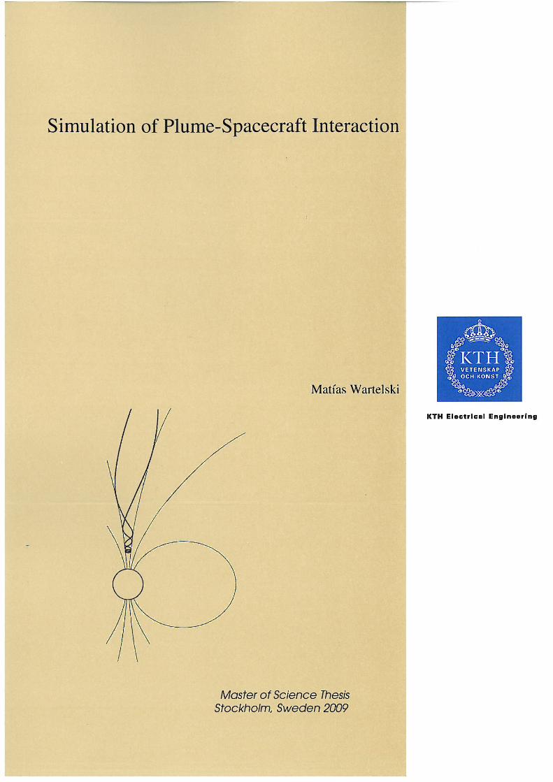
so equation (2.37) can be rewritten in terms of the total and translational energies(the two expressions are equivalent)
PEc;Et = PEt;Ei = cstE3=2�!t (Ec � Et)
��1expf�Ec=(kT )g: (2.39)
Here, the e�ective temperature T is de�ned by the total energy Ec of the collisionpair. This means that in equation (2.39), the exponential depends only on the totalenergy Ec but is independent on how this energy is distributed between translationaland internal energies. As total energy is conserved, the exponential is a constantparameter of the collision.
Consequently, in a collision where the total (and constant) energy is Ec, the prob-ability, for the collision pair, of having a particular value Et of the total translationalenergy can be rewritten, from equation (2.39), as
PEc;Et = cstE3=2�!t (Ec � Et)
��1: (2.40)
The maximum value of this probability is
(PEc;Et)max = cst (3=2� !)3=2�!(� � 1)��1f(� + 1=2� !) + Ecg�+1=2�!: (2.41)
and is obtained whenEt
Ec=
3=2� !
� + 1=2� !: (2.42)
The acceptance-rejection method detailed in section 2.6 can be applied to obtaina value of the post-collision translational and internal energies. A value E�t is chosenat random from the range 0 to Ec. The probability P of E�t is evaluated according toequation (2.40). Then the ratio P=Pmax is evaluated following equation (2.41) andcompared with a random fraction Rf that is generated from a uniform distributionbetween 0 and 1. If the probability ratio is greater than Rf , this value E
�t is employed
for the collision, but a new value is chosen and the process repeated if the ratio isless than Rf . Once a certain value E�t has been accepted, the post-collision internalenergy E�i is deducted as E�i = Ec � E�t . This is how the interchange betweentranslational and internal energy is performed.
The following step is to divide the internal energy between the two molecules.This is done using again the acceptance-rejection method in a similar way. In thisprocess, the post-collision total internal energy E�i is a constant and the probabilityP that molecule 1 has a post-collision internal energy ��i;1 is
P��i;1 = cst (��i;1)�=2�1(E�i � ��i;1)
�=2�1: (2.43)
The maximum probability occurs when the internal energy is equally divided be-tween the two molecules and the ratio P��i;1=Pmax is evaluated from this. Theacceptance-rejection method is again used to divide the post-collision translationalenergy.

2.5. SURFACE INTERACTIONS 17
The post-collision relative speed in the center of mass frame of reference, wherem = m1 = m2, is
c�r = (2E�t =mr)1=2 = 2(E�t =m)1=2: (2.44)
The direction for this speed, i.e. the de�ection due to collision, is chosen at randomfor the VHS and hard sphere models, from equation (2.30) for the VSS model.
2.5 Surface interactions
2.5.1 Equilibrium interaction
There are two models for the interaction of a stationary equilibrium gas with a solidsurface that maintain equilibrium between the surface and the gas. The �rst isspecular re�ection, where the molecular velocity normal to the surface is reversed,while its velocities parallel to the surface remain the same. Specular re�ection is aperfectly elastic interaction because the incident and re�ected molecules have thesame energy. A molecule with mass m, impinging on a surface with a speed u andan angle � to the surface, and being re�ected specularly, transmits to the surface anormal momentum equal to 2musin�. The macroscopic force per unit surface isobtained by calculating the normal momentum �ux, which is an integration of theabove formula over all molecules.
In di�use re�ection, which is the alternative model, the velocity of each moleculeafter re�ection is independent of its initial velocity. The velocities of the re�ectedmolecules as a whole are distributed in accordance with a the temperature of thegas, which must be the same as the surface temperature to be in equilibrium. Theprobability P� for a molecule to be re�ected with an angle � to the surface is
P� = (1=�)sin(�): (2.45)
This probability is maximal for � = �=2, i.e. in the normal direction to the sur-face, and no molecules are re�ected parallel to the surface. The factor 1=� is fornormalization.
When a gas with a free-stream pressure p1 and whose molecules are all re�ecteddi�usely, it can be shown that the e�ective pressure on the surface is
pdiff =2
3p1: (2.46)
2.5.2 Non-equilibrium interaction
The majority of realistic problems involve non-equilibrium interaction of a gas witha solid surface. As soon as the gas have some stream velocity relative to the surface,its stagnation temperature, which rules the gas-surface interaction, di�ers from thestatic temperature of the gas. Also, the surface temperature may di�er from oneof these. Therefore, the gas can not be in equilibrium with the surface and the
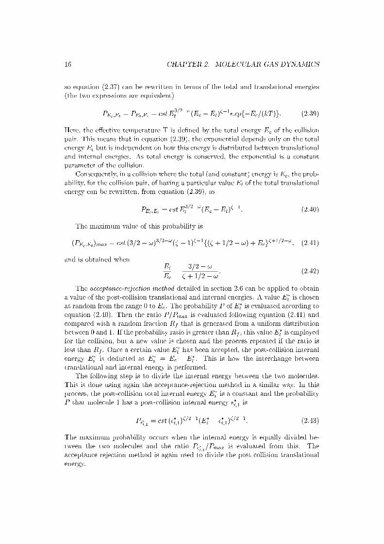
18 CHAPTER 2. MOLECULAR GAS DYNAMICS
distribution function of the incident molecules will di�er from that of the re�ectedmolecules.
The most common models used in engineering contexts for non-equilibrium in-teraction are empirical generalizations of the di�use and specular models.
Firstly, the di�use model is generalized. It is assumed that the incident andre�ected molecules are distributed in accordance with two di�erent temperatures Tiand Tr respectively, while the surface has its own temperature Tw. It is natural tothink that the re�ected gas, in comparison with the incident one, will tend to adjustits temperature to the surface temperature. The extent of this adjustment is givenby the thermal accommodation coe�cient
ac = (qi � qr)=(qi � qw) (2.47)
where qi and qr are respectively the incident and re�ected energy �uxes. qw is theenergy �ux corresponding to di�use re�ection in the equilibrium situation, withTr = Tw. The accommodation coe�cient goes from 0, for no accommodation at all,to 1, for complete thermal accommodation.
An extension of this model is a combination of di�use and specular re�ections.A fraction � of the molecules are re�ected specularly while the rest are re�ecteddi�usely.
2.6 The Monte-Carlo procedure and the
acceptance-rejection method
The Monte-Carlo method refers to a family of computational algorithms that relyon repeated random sampling to compute their results. They are used to simulatephysical and mathematical processes when an analytical solution is not availableand when this kind of probabilistic method will simulate with su�cient accuracythe real solution.
Imagine that one wants to know the value of a variable x after a physical ormathematical process and no analytical solution is available, but the distributionfunction of the variable is known. Assume the availability of a set of successiverandom fractions Rf that are uniformly distributed between 0 and 1. The probabilityfor the variable x of laying between x and x+ dx is given, thanks to the normalizeddistribution function, by
Px = fxdx: (2.48)
If the possible values for the variable x range from a to b, the total probability is
Z b
afxdx = 1: (2.49)
The cumulative distribution function is de�ned as
Fx =
Z x
afxdx: (2.50)

2.6. THE MONTE-CARLO PROCEDURE 19
Then a random value Rf is generated and Fx is set equal to Rf .Consider, for example, the case in which x is uniformly distributed between a
and b. Thenfx = 1=(b� a): (2.51)
andFx = (x� a)=(b� a) = Rf : (2.52)
This leads tox = a+Rf (b� a): (2.53)
This method is called the inverse-cumulative method and can only be used whenequation (2.52) can be inverted to express an explicit function of x.
Consider now the distribution function f 0u for a thermal velocity component inan equilibrium gas,
f 0u = (�=�1=2)expf��2u02): (2.54)
This givesF 0u = 1=2f1 + erf(�u0)g: (2.55)
This expression can not be inverted to express u0 in terms of Rf so the inverse-cumulative methods can not be used. The alternative is to use the acceptance-
rejection method.The distribution function is normalized by its maximum value fmax to give
f 0x = fx=fmax: (2.56)
A value of x is chosen at random from its possible range of values. The corre-sponding function f 0x is calculated and a random value Rf is again generated between0 and 1. The value of x is accepted if f 0x is greater than Rf . Else it is rejected andthe process repeated until a value is accepted.


Chapter 3
DS3V: interfacing of a DirectSimulation Monte-Carlo code foran industrial application
3.1 Software overview
Direct simulation methods model the real gas by a large number of simulatedmolecules in a computer. The position coordinates, velocity components, and in-ternal state of each of the simulated molecules are stored in the computer and aremodi�ed with time as the molecules are simultaneously followed through representa-tive collisions and boundary interactions in simulated physical space. DSMC refersto a family of direct simulation methods that use the Monte-Carlo procedure de-scribed in section 2.6 to simulate some physical phenomena.
The DS3V code has been developed by Graeme A. Bird, Emeritus Professorof Aeronautics at the University of Sydney. He �rst developed 2D and 2D axiallysymmetric DSMC codes and then released a fully 3D version of the method. DS3V2.6 is the latest version. It has been found to match the Astrium requirementsspeci�ed in chapter 1. Consequently, it has been interfaced with Astrium tools andis currently being used for analysis on Astrium spacecraft. Figure 3.1 shows the �lehierarchy during the interfacing procedure.
The simulation starts with the geometry de�nition. The user creates a 3D geom-etry with a 3D modeler; we used RHINOCEROS 4.0. The model is then exportedinto the .raw format, required by DS3V 2.6. After this, the user uses a DS3V inter-face, launched by the executable DS3DG.EXE, to de�ne the properties of all surfacesde�ned by the geometry �le. The two main types of surfaces are solid surfaces and�ow entry (in�ow) surfaces. In�ow surfaces are boundaries that the user employs tointroduce a �ow. They are meshed with triangles and the user can specify di�erent�ow properties in each triangle; this allows the introduction of any �ow. Once thegeometry is completely speci�ed and the in�ow properties (velocity, density, temper-ature) are set, the second DS3V interface, launched by the executable DS3V.EXE,
21

22CHAPTER 3. DS3V: INTERFACING OF A DIRECT SIMULATION
MONTE-CARLO CODE FOR AN INDUSTRIAL APPLICATION
Figure 3.1: File hierarchy for a DS3V simulation
can be used to de�ne the molecular properties (molecular mass, molecular diame-ter, viscosity, number of internal degrees, etc). This includes both molecular andmacroscopic properties of the �ow. Finally, the simulation starts.
Once the DS3V was chosen, the following step of this internship consisted inwriting FORTRAN routines to interface DS3V with PLUMFLOW, which is theAstrium tool that calculates the �ow �eld from a chemical thruster. By readingthe geometry �les, these routines compute the relative position and orientation ofthe in�ow surfaces to the thruster. At the same time, they read the PLUMFLOWoutput �les containing the �ow �eld information. Finally, they input or write the�ow properties (density, pressure, temperature...) in each of the mesh triangles ofthe in�ow surfaces.
Concerning the simulation method, one of its essential approximations is theuncoupling, over a small time step, of the molecular motion and the intermolecular

3.2. SIMULATION METHOD 23
collisions. All the molecules are moved (including the computation of the resultingboundary interactions) over the distances appropriate to this time step, followed bythe calculation of a representative set of intermolecular collisions. The time stepshould be small (for example �ve times smaller) compared with the mean collisiontime.
The Monte-Carlo probabilistic selection of representative collisions is based di-rectly on the relations that form the basis of kinetic theory, see sections 2.3 and 2.4,and on the acceptance-rejection method, see section 2.6.
The physical space is divided in cells used to facilitate the choice of moleculespairs for collisions and also for the sampling of the macroscopic �ow properties.The velocity space information is all contained in the positions and velocities of thesimulated molecules and not in the cells.
The microscopic boundary conditions are speci�ed by the behaviour of the indi-vidual molecules, see section 2.5, and not in terms of the distribution function. TheDSMC method employs simulated molecules of the correct physical size but theirnumber is reduced to a manageable level by regarding each simulated molecule asrepresenting a �xed number of real molecules.
The macroscopic boundary conditions are usually speci�ed as a uniform gas atzero time. The �ow develops from this initial state with time in a physically realisticmanner, rather than by iteration from an initial approximation to the �ow.
3.2 Simulation method
3.2.1 Molecular model
Through the DS3V user's interface, the user speci�es a number of parameters for themolecular model. Regarding elastic collisions, DS3V o�ers the possibility of usingthe hard sphere model described in section 2.3.5, the VHS model of section 2.3.6 orthe VSS model of section 2.3.7. The classical Larsen-Borgnakke model explained inparagraph 2.4.1 is used for inelastic collisions, whose number is controlled by thespeci�cation of a relaxation collision number.
The interaction between the gas and the solid surfaces is computed at the molec-ular level. This means, for example, that to calculate the pressure on the surface,the program calculates the momentum transmitted for each molecule to the wall,instead of using distribution functions and macroscopic properties. The interactionis a combination of specular and di�use re�ections, see 2.5, controlled by the userwho enters the fraction of molecules being re�ected specularly. If some moleculesare re�ected di�usely, the user must also specify the accommodation coe�cient.
3.2.2 Mean collision rate: the New Time-Counter (NTC) method
The mean collision rate � is the inverse of the mean collision time and is given byequation (1.10) in [6]
� = n�T cr (3.1)

24CHAPTER 3. DS3V: INTERFACING OF A DIRECT SIMULATION
MONTE-CARLO CODE FOR AN INDUSTRIAL APPLICATION
where n is the density, �T is the total collision cross-section and the cr is the relativevelocity. A bar over a quantity denotes averaged value over all molecules in thesample. The total number of collisions per unit time and unit volume is therefore
NC =1
2n � � =
1
2n2�T cr (3.2)
where the factor 1/2 is introduced to take into account that a collision involves twomolecules.
The mean free path is the average distance, in the frame of reference movingwith the stream, traveled by a molecule between collisions. It is obtained from themean thermal speed and the mean collision rate
� = c0=� =c0
n�T cr(3.3)
The goal is to �nd a procedure that best approaches this collision rate by beingas e�cient, from the computation point of view, as possible.
The mean value of the product �T and cr is calculated in each cell. Then thenumber of collisions in the cell at each time step would be NC�t. The collision pairswould then be chosen by the acceptance-rejection method using the probability �T cr.This procedure would have a computation time proportional to the total number ofmolecules in the cell.
Consider a cell of volume VC withN simulated or big molecules. If the gas densityat the cell position is n, then each simulated molecule represents FN = nVC=N realmolecules. Then choose a random pair of molecules with a relative speed cr betweenthem and a total cross-section �T . In the frame of reference of the �rst molecule,the second molecule is moving with speed cr. If the �rst molecule happens to fallinside the volume swept by the total cross-section moving at a speed cr, the collisiontakes place. Therefore, the probability P of collision between these two moleculesis given by the ratio between the swept volume mentioned above to the volume ofthe cell,
P = FN�T cr�t=VC (3.4)
The full set of collisions could be calculated selecting all N(N �1)=2 pairs in thecell and computing the collisions with a probability P . This is ine�cient because thenumber of potential collisions is proportional to the square of N and the probabilityP is often very small, so a lot of computation time will be lost computing pairs thatwill not collide. Here is where the NTC procedure appears.
Among all the pairs, the maximum value for �T cr is estimated. This gives themaximum probability for a collision to happen:
Pmax = FN (�T cr)max�t=VC (3.5)
Instead of selecting all possible N(N�1)=2 � N2 pairs, only a fraction 1
2N2Pmax
of pairs is selected. The collision for each of these pairs is computed with theprobability
Pcoll =�T cr
(�T cr)max(3.6)

3.2. SIMULATION METHOD 25
In other words, only a fraction Pmax of the total possible pairs are selected but,as the selected pairs are computed with a probability Pmax times higher, the �nalcollision rate remains the same while the computing procedure has turned muchmore e�cient. Indeed, the number of selected pairs is
1
2N2Pmax =
1
2N2FN (�T cr)max�t=VC =
1
2Nn(�T cr)max�t (3.7)
Therefore, the computing time is linear with N and not N2 as before.
3.2.3 Meshing the �ow �eld space
The 2.6 version of DS3V divides the physical space into two di�erent cell networks.The �rst network is called by Bird "cell system" or "sampling cells" and is
only used for the sampling of the macroscopic properties. In other words, givena cell, DS3V evaluates all the macroscopic properties in this cell by averaging theappropriate quantities over all the simulated molecules contained by this volume cell.So the macroscopic properties have one value in each cell. Therefore, the cell sizeis the space resolution of �ow properties. For this reason, a typical cell dimensionshould be small compared with the distance over which there is a signi�cant changein the �ow properties.
The second network is called "sub-cells system" or "collision cells". When acollision is to be calculated, a molecule for the potential collision is chosen at randomfrom a collision cell. If the number of molecules in the collision cell is less than 30,the nearest molecule is chosen as the potential collision partner. For larger number,a new transient rectangular grid generated in the collision cell and the size of thegrid elements is such that there is approximately one molecule per grid element.When there is more than one molecule in a grid element, the two molecules arechosen as collision partners. These are called the nearest-neighbour procedures.According to Bird [6], they assure that the ratio of the mean separation betweencollision partners one time step before the collision (m.c.s) to the mean free pathm:c:s� is small compared with unity over the �ow �eld, typically less than 0.2.The macroscopic properties are supposed to have no in�uence at the molecular
level. This is not completely true because the "sampling cells" are used to establishthe collision rate.
3.2.4 Time step
The time step should be much less than the mean collision time tcol. In this way,the program would neglect no collisions. However, the mean collision time may varya lot in the di�erent regions of a �ow �eld because it depends on many factors suchas number density and molecules velocity. For this reason, it would not be e�cientto use a single value for the time step over the whole �ow �eld. Consequently, fore�ciency reasons and also to ensure that the parameter m:c:s
� is small compared withunity over the �ow �eld, DS3V 2.6 uses a di�erent time step for each molecule andevery cell.

26CHAPTER 3. DS3V: INTERFACING OF A DIRECT SIMULATION
MONTE-CARLO CODE FOR AN INDUSTRIAL APPLICATION
The mean collision time is calculated and stored in each sample cell. Eachmolecule has its own time step: faster molecules have smaller time steps and vice-versa. Consider a collision pair of molecules 1 and 2 with velocities v1 and v2 andwith molecule time steps �1 and �2 respectively. The maximum separation betweenthe two molecules just before the collision is obtained when they move one towardsthe other with opposite velocities. In the simulation, the molecules do not have acontinuous, but a discretized movement. The position of the molecules previous tothe collision is therefore
d12 = v1 ��t1 + v2 ��t2: (3.8)
It is natural to de�ne the molecular time steps such that all molecules in the samecell travel the same distance during their respective time step so
v1 ��t1 = v2 ��t2 (3.9)
sod12 = 2v1 ��t1: (3.10)
To ensure the condition on the mean separation between collision partners, thefollowing inequation must be veri�ed
m:c:s
�=
d12�
=2v1 ��t1
�� 0:2 (3.11)
or
�t1 �0:1 � �
v1: (3.12)
Therefore, every molecule, with speed v, has a time step �tmol such that
�tmol =0:1 � �
v: (3.13)
and using the mean free path equation (3.3), we obtain
�tmol =0:1
�
c0
v: (3.14)
As c0
v is of the order of unity, the �nal result is
�tmol '0:1
�=
1
10tcol: (3.15)
The overall time variable is advanced in time steps smaller than smallest moleculetime step in the whole �ow �eld. However, only a small fraction of molecules aremoved at each overall time step: those molecules whose corresponding time variablefalls one tenth behind the overall time variable.
On the other side, each collision cell has a time variable that is advanced withsteps equal to the mean collision time in the cell. In a collision cell, only when thecell time variable falls one tenth behind the overall time variable, the collisions arecalculated.

3.3. GENERATION OF THE 3D GEOMETRY FILE 27
3.2.5 Number of simulated molecules
The user is obliged to specify a density for the main �ow stream. This density is usedby DS3V to make a rough evaluation of the scale length of the macroscopic propertiesgradients. This gives the size of the sample cells, which are all equal more or less.From the size of the sample cells, the program evaluates, in average, the minimumnumber density of simulated molecules necessary for a good statistical simulation:the temperature in a cell with only two simulated molecules has no physical sense.Finally, using the maximum allocated RAM and this minimum number density ofsimulated molecules, DS3V determines a �xed ratio of real molecules to simulatedmolecules. This ratio is the number of real molecules represented by each simulatedmolecule.
This ratio, of the order of 1014 to 1018, is more or less uniform over the whole�ow�eld. This is such because the program is intended in principle for studiesof interaction between uniform �ows and solid bodies. Thruster plumes are verydi�erent: the regions close to the plume axis are high-density regions while theregions far are low-density regions. This is problematic because it means that thecells in the dense regions will be over-populated by simulated molecules while thecells in the rare�ed regions will be under-populated. Over-population does notdamage the quality of a DSMC simulation, but it slows it down dramatically. Under-population, on the contrary, will lead to unphysical results because the statistics areof bad quality.
The solution chosen by Bird to overcome this problem is the option "Adapt cells"
3.2.6 Adapting cells
The �ow�eld space is meshed uniformly when the simulation is launched for the �rsttime because there is no data concerning where the dense and the rare�ed regionswill be. On the contrary, this is known once the simulation has been running for acertain time. Consequently, the cells can be adapted in terms of size to include acertain number of simulated molecules and thus provide results with physical sense.In this process, the user can specify the average number of simulated molecules to becontained in each "sample cell" and in each "collision cell" and the program meshesagain the �ow�eld space. Bird [7] recommends 7 molecules per collision cell.
3.3 Generation of the 3D geometry �le
The 3D geometry �le is generated with several steps:
- First the .raw �le is generated. This �le only contains the meshed geometryand in�ow boundaries.
- Then the routine count.exe pre-processes the .raw �le to give it the formatrequired for input of DS3DG.EXE and renames it DS3TD.DAT.

28CHAPTER 3. DS3V: INTERFACING OF A DIRECT SIMULATION
MONTE-CARLO CODE FOR AN INDUSTRIAL APPLICATION
- Finally DS3DG.EXE is run and the user speci�es for each surface if it must beconsidered as solid or in�ow surface.
These three steps are presented in the following paragraphs.
3.3.1 Generation of the .raw �le
Basic steps
In principle, any geometrical form is accepted by DS3V. However, some conditionsmust be respected:
1) The simulation is performed by DS3V in a parallelepiped domain, whoseboundaries are speci�ed by the user in the last step before starting the simulation.The 3D geometry must consist of:
- Closed surfaces: these surfaces must lay completely within the parallelepipeddomain (excepted for in�ow boundaries).
- Open surfaces: these surfaces must start and �nish on the �ow �eld boundaries
2) The surfaces must be meshed with triangles.
3) The FORTRAN routines require that all surfaces names begin by "Object".
4) The 3D geometry must be exported as a .raw �le. In order to do that, every-thing in the 3D model must be suppressed except the meshes.
In�ow surfaces
The entry �ow or in�ow surfaces are the key point of DS3V interfacing with PLUM-FLOW that calculates the �ow �elds of chemical thrusters. These surfaces, like allthe other surfaces de�ning the geometry, are meshed with triangles. The FOR-TRAN routine DS3VPR.EXE, described in �5.2, reads and calculates the centre ofeach in�ow triangle. Then, it reads the properties of the �ow �eld at this loca-tion in the .FLOW �le. Finally, these properties are written for each triangle inthe DS3SD.DAT �le, which is used as input for the DSMC simulation. This allowsDS3V.EXE to simulate a chemical thrusters plume entering the calculation volumethrough the in�ow triangles.
Therefore, the in�ow surfaces must be de�ned in a smart and e�cient way: themesh size determines the scale length of the �ow properties gradients. There aretwo kinds of in�ow surfaces: closed and open surfaces.
3.3. GENERATION OF THE 3D GEOMETRY FILE 29
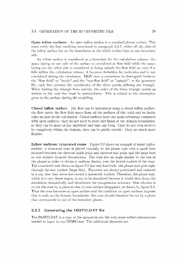
Open in�ow surfaces An open in�ow surface is a standard planar surface. Thismust verify the �rst condition mentioned in paragraph 3.3.1: either all the sides ofthe in�ow surface lay on the boundaries or the whole surface lays on one boundaryside.
An in�ow surface is considered as a boundary for the calculation volume: thespace laying on one side of the surface is considered as �ow �eld while the spacelaying one the other side is considered as being outside the �ow �eld so, even if itfalls within the calculation volume, it becomes forbidden for molecules and is notconsidered during the simulation. DS3V uses a convention to distinguish betweenthe "�ow �eld" or "inside" and the "non-�ow �eld" or "outside": in the geometry�le, each line contains the coordinates of the three points de�ning one triangle.When looking the triangle from outside, the order of the three triangle points aswritten in the .raw line must be anticlockwise. This is related to the orientationgiven to the surface during 3D modelling.
Closed in�ow surface The �ow can be introduced using a closed in�ow surface:the �ow enters the �ow �eld space from all the surfaces of this solid and its insidetakes no part in the calculation. Closed surfaces have one main advantage comparedwith open surfaces: they do not need to start and �nish at the domain boundaries,so they can be more or less anywhere and take any form. They do not even need tobe completely within the domain, they can be partly outside. They are much more�exible.
In�ow surfaces: truncated cones Figure 3.2 shows an example of smart in�owsurface: a truncated cone is placed coaxially to the plume axis with a small basesituated between the thruster ankle point and thruster exit point and the large baseor exit surface situated downstream. The cone has an angle similar to the one ofthe plume in order to obtain a uniform density over the lateral surface of the cone.The truncated cone shown in �gure 3.2 has one drawback: the plume axis goes rightthrough the exit surface (large disc). Thrusters are always positioned and orientedin a way that they never �re toward a spacecraft surface. Therefore, the plume axis,which is a very dense region, is not to be simulated because it would slow down thesimulation dramatically and deteriorate the computation accuracy. One solution isto cut the cone by a plane so that its exit surface disappears, as shown by �gure 3.3.Thus the cone becomes an open surface and the condition on open surfaces imposesthat it ends on the domain boundaries: the cone should therefore be cut by a planethat corresponds to one of the boundary planes.
3.3.2 Generating the DS3TD.DAT �le
The DS3TD.DAT is a copy of the geometrie.raw �le with some added informationsneeded as input to run DS3DG.exe. The additional elements are:

30CHAPTER 3. DS3V: INTERFACING OF A DIRECT SIMULATION
MONTE-CARLO CODE FOR AN INDUSTRIAL APPLICATION
Figure 3.2: Closed in�ow surface: truncated cone
- A line at the top of the �le containing the total number of surfaces.
- For each surface, the number of triangles is written instead of the surface namebeginning with the word "Object".
Basic steps
To generate the DS3TD.DAT �le, the following steps have to be done:
1) The .raw �le containing the 3D geometry is renamed manually "geome-trie.raw". The extension .raw must be kept.
2) This �le has to be copied into the folder containing the FORTRAN count.exeroutine.
3) The routine count.exe is run from a Linux machine.
4) The new �le DS3TD.DAT is generated by count.exe.

3.3. GENERATION OF THE 3D GEOMETRY FILE 31
Figure 3.3: Truncated cone cut open to avoid simulating the dense plume axis
3.3.3 Generating the DS3TD.DAT
The basic steps to generate the DS3TD.DAT �le are the following:
1) The DS3TD.DAT �le is copied into the folder containing the DS3DG.EXEprogram.
2) The DS3DG.EXE program is run in Windows.
3) The user speci�es the number of species in the gas.
4) For each mesh triangle, the user speci�es if it is a "Solid surface triangle withspecies-independent properties" or an "In�ow triangle".
5) a) For an In�ow Triangle, the panel shown in �gure 3.4 will follow. Theuser must only enter the "Fraction of Species" and set the "Flow stop time" to avalue su�ciently high compared with the virtual simulation duration (not the realsimulation time, but the �nal value of the time variable in the simulation). Usuallya few seconds is enough because the time variable does not usually reach 1 second.All the other parameters of the in�ow triangle are �ow �eld information that will

32CHAPTER 3. DS3V: INTERFACING OF A DIRECT SIMULATION
MONTE-CARLO CODE FOR AN INDUSTRIAL APPLICATION
be set automatically by the FORTRAN routine ds3vpr.exe.
Figure 3.4: Input parameters for an In�ow Triangle
b) For a solid surface triangle, the gas-surface interaction parameters (absorp-tivity, specularity,...) are speci�ed.
6) Once the operation is done for all mesh triangles, the �le DS3SD.DAT isgenerated.
3.4 Interfacing with the �ow �eld �le
Figure 3.5 shows an example of plume �ow �eld computed with PLUMFLOW. Tointerface DS3V program with the �ow �eld �le, the following steps have to be done:
- Creation of the input �les (thruster and PARAM.FOR �les).
- Run of the ds3vpr.exe routine.
These two steps are presented in the following paragraphs.

3.4. INTERFACING WITH FLOW FIELD 33
Figure 3.5: PLUMFLOW computation
3.4.1 Input �les
The thruster �le
Figure 3.6 shows an example of thruster �le.
Figure 3.6: Example of thruster �le
The di�erent elements are de�ned as follows:
34CHAPTER 3. DS3V: INTERFACING OF A DIRECT SIMULATION
MONTE-CARLO CODE FOR AN INDUSTRIAL APPLICATION
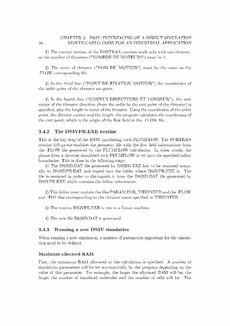
1) The current version of the FORTRAN routines work only with one thruster,so the number of thrusters ("NOMBRE DE MOTEURS") must be 1.
2) The name of thruster ("NOM DU MOTEUR") must be the same as the.FLOW corresponding �le.
3) In the third line ("POINT DE FIXATION MOTEUR") the coordinates ofthe ankle point of the thruster are given.
4) In the fourth line ("COSINUS DIRECTEURS ET LONGEUR"), the unitvector of the thruster direction (from the ankle to the exit point of the thruster) isspeci�ed, plus the length in meter of the thruster. Using the coordinates of the anklepoint, the director cosines and the length, the program calculates the coordinates ofthe exit point, which is the origin of the �ow �eld in the .FLOW �le.
3.4.2 The DS3VPR.EXE routine
This is the key step of the DS3V interfacing with PLUMFLOW. The FORTRANroutine ds3vpr.exe enriches the geometry �le with the �ow �eld informations fromthe .FLOW �le generated by the PLUMFLOW calculation. In other words, theplume from a thruster simulated with PLUMFLOW is set into the speci�ed in�owboundaries. This is done in the following steps:
1) The DS3SD.DAT �le generated by DS3DG.EXE has to be renamed manu-ally to DS3SDPR.DAT and copied into the folder where DS3VPR.EXE is. The�le is renamed in order to distinguish it from the DS3SD.DAT �le generated byDS3VPR.EXE which contains the in�ow information.
2) This folder must contain the �les PARAM.FOR, THRUSTER and the .FLOWand .TO7 �les corresponding to the thruster name speci�ed in THRUSTER.
3) The routine DS3VPR.EXE is run in a Linux machine.
4) The new �le DS3SD.DAT is generated.
3.4.3 Running a new DS3V simulation
When running a new simulation, a number of parameters important for the simula-tion need to be de�ned.
Maximum allocated RAM
First, the maximum RAM allocated to the calculation is speci�ed. A number ofsimulation parameters will be set automatically by the program depending on thevalue of this parameter. For example, the larger the allocated RAM will be, thelarger the number of simulated molecules and the number of cells will be. The

3.4. INTERFACING WITH FLOW FIELD 35
maximum RAM depends on each PC, so each user should �nd out the limitations ofhis own computer. It has to be noted that DS3V 2.6 can only be run on 32 bit PC,so the maximum RAM must be less than 2Gb. Nevertheless, it has been observedthat, in practice, for allocated RAM higher than 1024Mb, the simulation bugs.
However, it is not always worthy to use the maximum possible memory because,although this leads to a more accurate simulation, it also slows down the calculation.
Flow �eld limits
The speci�cation of the "Flow Computation Region" must respect the rules ex-plained in paragraph 1) of section 3.3.1. The window shown in �gure 3.7 is used toset the domain boundaries.
Figure 3.7: Setting the �ow �eld boundaries
Setting the gas properties
The gas properties can be speci�ed by the user by choosing the "Custom Compo-sition" option or set automatically by choosing one of the standard gases. Then,the molecular properties are speci�ed in the DS3V interface, see �gure 3.8(b). The

36CHAPTER 3. DS3V: INTERFACING OF A DIRECT SIMULATION
MONTE-CARLO CODE FOR AN INDUSTRIAL APPLICATION
"Reference diameter of the molecule", the "reference temperature", the "Viscosity-temperature power law" and the "Molecular mass", must be read by the user in the.T07 �le (generated by PLUMFLOW) and they are found in the positions shown in�gure 3.8(a).
Properties of the main stream
DS3V o�ers the user the possibility of simulating a homogeneous stream. However,this option is not used when analyzing plume-spacecraft interaction because theplume of a thruster is never a homogeneous stream. Nevertheless, when DS3Vestimates the number of real molecules represented by a simulated molecule, it usesthe "Main Stream Properties" as reference properties. The most important of theseparameters is the "Number Density". For example, a high number density will makeevery simulated molecule to represent a large number of real molecules. Therefore,the user should specify parameters representative of the plume.
Boundary conditions
The calculation volume is a parallelepiped. The user attributes boundary propertiesto each of the six surfaces de�ning the parallelepiped: they can be outside the �ow,a plane of symmetry, a stream boundary or a vacuum interface.
Initial conditions
There are two main options for the initial conditions: the initial �ow is a vacuumor the reference stream de�ned by the user.
3.4.4 Division of the domain
After setting the parameters, DS3V.EXE enters a calculation phase in which it di-vides the �ow �eld in a number of divisions, sampling cells and collision cells. Thethree steps are the following:
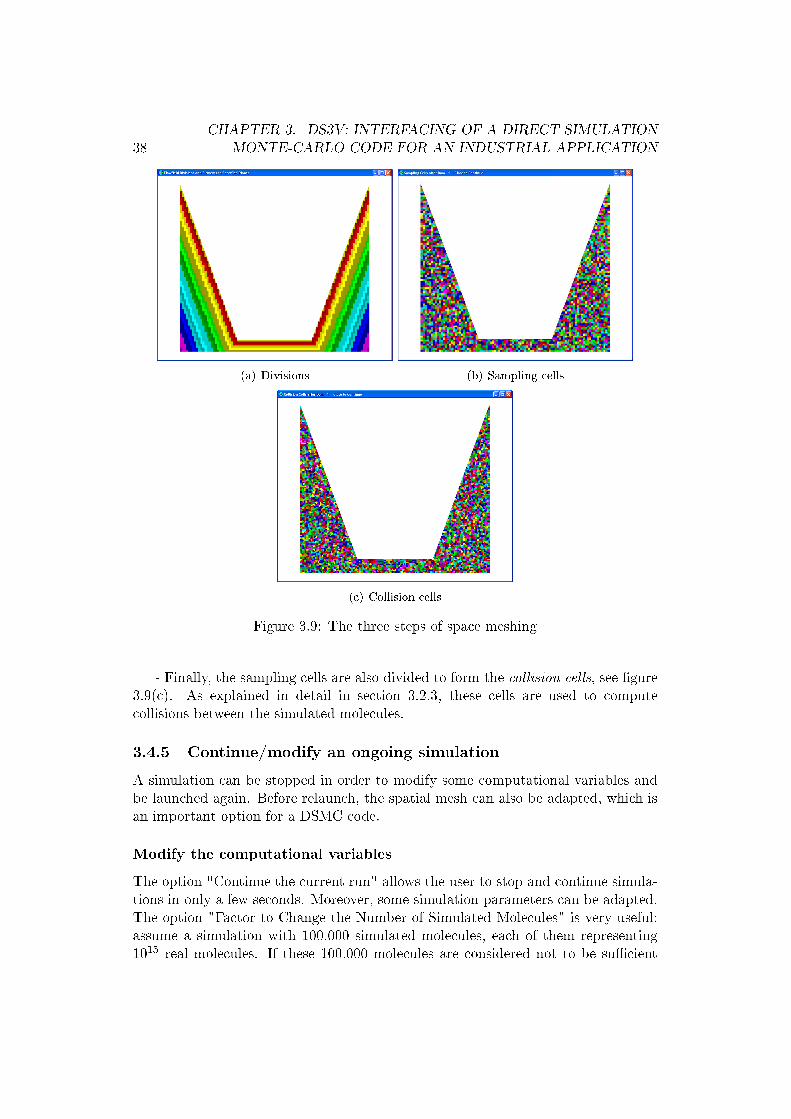
- In the �rst step, DS3V divides the calculation volume in a number of divisions.The colored divisions, see �gure 3.9(a), correspond to �ow �eld regions accessi-ble to molecules and the di�erent colors indicate how far a division is from solidboundaries. This is important for simulation because only in divisions considered tobe su�ciently close to a solid boundary will �ow-surface interaction be computed.The white regions are those laying inside a solid, so these regions are forbidden tomolecules.
- In the second step, the divisions are redivided to form the sampling cells, see�gure 3.9(b), which are used for computation and visualization of �ow macroscopicproperties.

3.4. INTERFACING WITH FLOW FIELD 37
(a) Mean molecular properties in the .T07 �le
(b) DS3V interface for molecular properties input
Figure 3.8: Read and input of the molecular properties
38CHAPTER 3. DS3V: INTERFACING OF A DIRECT SIMULATION
MONTE-CARLO CODE FOR AN INDUSTRIAL APPLICATION
(a) Divisions (b) Sampling cells
(c) Collision cells
Figure 3.9: The three steps of space meshing
- Finally, the sampling cells are also divided to form the collision cells, see �gure3.9(c). As explained in detail in section 3.2.3, these cells are used to computecollisions between the simulated molecules.
3.4.5 Continue/modify an ongoing simulation
A simulation can be stopped in order to modify some computational variables andbe launched again. Before relaunch, the spatial mesh can also be adapted, which isan important option for a DSMC code.
Modify the computational variables
The option "Continue the current run" allows the user to stop and continue simula-tions in only a few seconds. Moreover, some simulation parameters can be adapted.The option "Factor to Change the Number of Simulated Molecules" is very useful:assume a simulation with 100.000 simulated molecules, each of them representing1015 real molecules. If these 100.000 molecules are considered not to be su�cient

3.4. INTERFACING WITH FLOW FIELD 39
to provide an accurate result, the total number of simulated molecules can be mul-tiplied by a factor chosen by the user. For example, a factor of 10 will lead thesimulation to employ 1.000.000 molecules and each of these will now represent 1014
real molecules. On the contrary, if the simulation if too slow because there are toomany simulated molecules, their number can be multiplied by a factor less than 1.
(a) Before adaptation (b) After adaptation
Figure 3.10: Collision cells in a DS3V simulation of a rare�ed gas �ow past a sphere
Cells adaptation
The initial division of the �ow �eld is done with cells of the same size because theprogram does not know how the �ow �eld will look before launching the simulation.Once the simulation has gone for a certain time, there may be regions with higherdensities and others with lower densities. In the high density regions, there willbe a lot of simulated molecules, while the low-density regions will have very few ofthese. However, in both regions the cell size is similar. The option "Adapt Cells andContinue" generates a new cells network in the domain, this time taking into accountthe density distribution. In the high-density regions, the sampling and collisioncells will be small, allowing catching the steep gradients of macroscopic propertieswhile keeping a su�cient number of simulated molecules per cell to assure a goodstatistics. In the low-density regions, the cells must be large to contain a su�cientlyhigh number of simulated molecules. See �gures 3.10(a) and 3.10(b) for an example:

40CHAPTER 3. DS3V: INTERFACING OF A DIRECT SIMULATION
MONTE-CARLO CODE FOR AN INDUSTRIAL APPLICATION
before adaptation, the cells size is uniform. After adaptation, that is no longer true:in the wake, the cells are clearly larger to counteract the low-density while the cellsin the stagnation and shock region are smaller than anywhere else to counteractthe high-density. Adapting the cells is an option that has physical meaning onlywhen the initial simulation has been running su�ciently so that the adaptation isbased on a �rst, although not so accurate, solution of the problem. When adaptingthe cells, the user has to specify the number of molecules per collision cell and thenumber per sampling cell (Bird [7] recommends 7).
3.4.6 Results output
The results can either be visualized using the DS3V visualization options, see �gure3.11, or written in output �les. There are two di�erent output �les, one contains�ow �eld information and another contains information of �ow-surface interaction.
Figure 3.11: DS3V visualization interface

Chapter 4
SYSTEMA/PLUME: a simpli�edapproach for plume impingementanalysis
4.1 Method overview
The SYSTEMA/PLUME tool is used to predict the plume impingement e�ects onany target geometry. The computation is begun with the de�nition of the geometryand location of the thrusters. Then, a plume �ow �eld previously computed by thePLUMFLOW module is selected. The selected thruster �le contains the followingcharacteristics of the plume �ow in the spatial vacuum:
- Physical properties of the gas: viscosity, heat capacity ratio ( ), speci�c heatcapacity and Prandtl number as a function of gas temperature.
- Thermodynamic properties of the plume: velocity, density, pressure, tempera-ture.
This information is used to calculate the e�ects produced by the plume impinge-ment on the spacecraft surfaces. This includes:
- Dynamic e�ects: pressure and shear stresses.
- Thermal e�ects: convective and radiative heat �uxes.
- Contamination: mass �uxes.
This is done by interpolation of the �ow �eld on the solid surface meshes. Themain physical assumption of this method is that the �ow is not modi�ed by the solidsurfaces so the interaction is calculated directly from the �ow properties predicted
41

42 CHAPTER 4. THE SYSTEMA/PLUME APPROACH
by PLUMFLOW at the surface positions. Once the �ow �eld has been interpolated,PLUME employs a number of equations based on the macroscopic �ow properties tocompute the e�ects on the surface. These equations are based on a major physicalassumption: the �ow is in the free-molecular regime. In space, a �ow becomesrare�ed quickly outside the thruster so this hypothesis matches the reality often.
4.2 Gas-surface interaction in the free-molecular regime
4.2.1 Interaction model
The model used, see [13], is an extended version of the combination of di�use andspecular re�ections described in section 2.5.2. A molecule can undergo three di�erentinteractions with a solid wall:- absorption, characterized by the absorptivity , which is the ratio of absorbedmass �ux to the incident mass �ux,- specular re�ection, characterized by the ratio � of specularly re�ected mass �ux tothe re�ected mass �ux,- di�use re�ection, characterized by the accommodation coe�cient ac de�ned insection 2.5.2.In other words, the model assumes that for an incident mass �ux _m,- the fraction _m is absorbed or gets stuck in the surface,- the fraction (1� )� _m is re�ected specularly,- the fraction (1� )(1��) _m is re�ected di�usely with an accommodation coe�cientac.
The absorption is always set to zero because of a lack of experimental data tocharacterize the absorptivity. Consequently, this parameter does not appear in theequations presented in the following paragraphs.
4.2.2 Impingement pressure
The impingement pressure is the e�ective force per unit surface applied to the bodyin the direction normal to the local surface. The absorption phenomenon beingignored here, the transmission of this force occurs through specular or di�use re-�ection of molecules. Under the assumption of free-molecular regime, the re�ectedmolecules from the body travel a very long distance before colliding with anothermolecule. The pressure applied on the surface is the sum of the pressures due to theincident and re�ected gases,
p = pi + pr: (4.1)
It must be remembered that the pressure is the normal momentum �ux to a surface(solid or �ctitious).
The incident molecules are assumed to be those of the equilibrium free-stream,and the corresponding pressure, i.e. the normal momentum �ux counted positively

4.2. GAS-SURFACE INTERACTION 43
when arriving to the surface, is given by equation (4.25) in [6],
pi2�21=�1 =
pip1
= [! exp(�!2) + �1=2f1 + erf(!)g � (1=2 + !2)]=�1=2 (4.2)
where s = c0p2RT1
is the molecular speed ratio and ! = s sin(�) = s cos(�) where
� is the angle of incidence of the stream velocity vector to the surface elementand � = �=2 � � is the angle of the stream velocity vector to the vector normalto the surface, and � = (2RT )�1=2. The subscript 1 is a direct consequence ofthe free-molecular regime assumption: it means that the incident �ow is the localundisturbed �ow.
The re�ected gas is considered �ctitiously as a gas emitted by the surface. Thenormal momentum �ux of this gas is equivalent to a pressure on the solid surfacethanks to the principle of action-reaction. Among the re�ected molecules, a fraction �is re�ected specularly and the rest is re�ected di�usely. The re�ected gas is thereforedivided in two gases with two pressures, so that the pressure of the re�ected gas iswritten as
pr = pr;spec + pr;diff : (4.3)
In specular re�ection, the solid boundary acts as a plane of symmetry, so thespecularly re�ected molecules have the same equilibrium distribution as the incidentmolecules. The pressure is linearly proportional to the gas density, so, as only afraction � out of the total number of incident molecules is re�ected specularly, thepressure of the gas re�ected specularly is
pr;spec = �pi: (4.4)
This means that the total impingement pressure pimp is
pimp = pi + pr;spec + pr;diff = (1 + �)pi + pr;diff : (4.5)
The last step is to express the pressure of the gas re�ected di�usely. This is donein two steps. Firstly, the mass �ux of the specularly re�ected gas is calculated usingthe principle of mass conservation: as no real molecules are absorbed nor emittedby the surface, the net number �ux to the surface element must be zero. Then,the accommodation coe�cient which controls the thermal equilibrium between thegas and the wall provides the temperature Tr;diff of these molecules. Finally, thecorresponding pressure pr is given by equation (4.2) for a stationary gas.
The net number �ux must be zero, so
_Nr;diff = _Ni � _Nr;spec = (1� �) _Ni (4.6)
where dot means time derivative.The incident gas is the free-stream gas, so the incident �ux is given by equation
(4.22) in [6]_Ni =
n12�1=2�1
[exp(�!2) + �1=2!f1 + erf(!)g]: (4.7)

44 CHAPTER 4. THE SYSTEMA/PLUME APPROACH
The di�usely re�ected gas is in a steady state in equilibrium with the wall, soits �ux is given by equation (4.24) in [6]
_Nr;diff =nr;diff
2�1=2�r;diff: (4.8)
The combination of equations (4.6), (4.7) and (4.8) gives the number density of thedi�usely re�ected gas as
nr;diff = (1� �)n1(T1=Tr)1=2[exp(�!2) + �1=2!f1 + erf(!)g] (4.9)
Usually, the accommodation coe�cient is set to 1 and the temperature Tr is thereforeTw. This provides in most cases the worst-case scenario (highest thermal �ux) andaccording to Bird [6], it appears to be adequate for the vast majority of practicalgas �ows. Bird [6] also says that there is no model of gas surface interactions givingTr;diff when � 6= 1 adequate for quantitative studies over a wide range of parameters.An empirical model is needed at this point.
Finally, equation (7.53) in [6] is used to obtain the pressure due to the portionof molecules re�ected di�usely:
pr;diff =nr;diffm
4�2r;diff
= (1� �)n1m
4�2r;diff(T1=Tr)
1=2[exp(�!2) + �1=2!f1 + erf(!)g](4.10)
so
pr;diffp1
=2�21pr;diff
�1
= (1� �)1
2(Tr;diff=T1)1=2[exp(�!2) + �1=2!f1 + erf(!)g]:
(4.11)
The impingement pressure normalized to the free-stream pressure is thus givenby combination of equations (4.5), (4.11) and (4.2) and coincides with equation(7.58) in [6]
pimp=p1 =h(1 + �)��1=2s sin�+ 1=2(1� �)(Tr;diff=T1)1=2
i� exp(�s2 sin2�)
+h(1 + �)(1=2 + s2 sin2�) + 1=2(1� �)(Tr;diff=T1)1=2�1=2s sin�
i��1 + erf(s sin�)
�(4.12)
where, for reminder, ! = s sin�. The terms with (Tr;diff=T1)1=2 are those relatedto di�use re�ection and the others are related to incident and specular re�ection.

4.2. GAS-SURFACE INTERACTION 45
4.2.3 Shear stress
Shear stress is the parallel momentum �ux to the surface. Like with pressure, thetotal shear stress � on the surface is the sum of the incident and re�ected shearstresses �i and �r
� = �i + �r (4.13)
where the re�ected shear stress is the sum of the
�r = �r;spec + �r;diff : (4.14)
For specular re�ection, equations 7.50 in [6] give
�r;spec = ��i (4.15)
so, in the general case where a fraction � of incident molecules are re�ected specularly
�r;spec = ���i: (4.16)
As the re�ected shear stress is zero in di�use re�ection, see equation (7.52) in [6],the total shear stress in our general case is
� = (1� �)�i: (4.17)
The shear stress due to incident molecules is the inward parallel momentum �ux
given by equation (4.26) in [6] as
�2�i=� = s cos� (� Ni=n): (4.18)
The incident number �ux is given by equation (4.7) which, combined with equations(4.18) and (4.17), gives the total shear stress (equation (7.61) in [6]):
�=p1 = ��1=2(1� �)s cos�hexp(�s2sin2�) + �1=2s sin�f1 + erf(s sin�)g
i:
(4.19)
4.2.4 Heat transfer
The total energy �ux is also the sum of the incident and re�ected energy �uxes,
q = qi + qr (4.20)
and again
qr = qr;spec + qr;diff : (4.21)
Like with the pressure, we have
qr;spec = �qi: (4.22)

46 CHAPTER 4. THE SYSTEMA/PLUME APPROACH
The incident thermal �ux is the sum of the inward translational energy �uxand the inward internal energy �ux given by equations (4.27) and (4.30) in [6]respectively. The sum of these expressions gives
�31qi=�1 =1
8�1=2[f2s2+
+ 1
� 1gexp(�s2cos2�)+2�1=2s cos�fs2+
� 1gf1+erf(s cos�)g]:
(4.23)The thermal �ux due to molecules re�ected di�usely can be related to the cor-
responding pressure by combining equations (7.53) and (7.54) in [6] to give:
qr;diff = + 1
� 1
pr;diff
2�1=2�r;diff(4.24)
so using equation (4.11) we obtain
2�31qr;diff�1
= ( + 1
� 1)(1� �)
1
4�1=2Tr;diffT1
[exp(�!2) + �1=2!f1 + erf(!)g]: (4.25)
Therefore, the total energy �ux is
2�31q=�1 =(1� �)=(2�1=2)(
�s2 + =( � 1) +
1
2( + 1)=( � 1)(Tr;diff=T1)
�
�hexp(�s2sin2�) + �1=2s sin�1 + erf(s sin�)
i
�1
2exp(�s2sin2�)):
(4.26)

Chapter 5
Back�ow impingement:comparison betweenSYSTEMA/PLUME and DS3V
5.1 Introduction
As explained in section 4.1, the SYSTEMA/PLUMEmethod assumes that the �ow isnot disturbed by solid structures. This is the main di�erence with the DSMCmethodused in the DS3V code. DS3V simulates real �ow-structure interactions because the�ow itself is modi�ed so the impingement e�ects on the structure depend on howthe structure itself has modi�ed the �ow. From the numerical point of view, theSYSTEMA/PLUME and DSMC methods are completely di�erent. While DSMCsimulates the movement of molecules, SYSTEMA/PLUME employs a number ofequations based on the macroscopic properties to compute the e�ects on the surface.These equations are based on the assumption that the �ow is in the free-molecularregime. When a surface is close to the thruster and the gas is not rare�ed enough,this hypothesis looses legitimacy. As the gas is modeled at the molecular level, theDSMC method makes no assumption concerning the �ow regime so in principle itis valid in the free-molecular, transitional and continuum regime.
All together means that the DSMC method is more accurate than the SYS-TEMA/PLUME approach. However, while a SYSTEMA/PLUME computationtakes some seconds, a DS3V simulation lasts from a few hours to a few days. There-fore, DS3V should only be used when it is clear that SYSTEMA/PLUME doesnot give accurate results. This chapter details a study case where both approacheswere compared in order to evaluate the accuracy of SYSTEMA/PLUME and alsoto understand the physical phenomena that might induce this approach to looseaccuracy.
A recurrent con�guration in Astrium satellites that requires plume impingementanalysis is that of a thruster ankled on one satellite's surface. Usually, the surfaceis a radiator and the magnitude of interest is the thermal �ux. During attitude
47
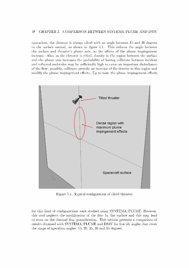
48 CHAPTER 5. COMPARISON BETWEEN SYSTEMA/PLUME AND DS3V
operations, the thruster is always tilted with an angle between 15 and 35 degreesto the surface normal, as shown in �gure 5.1. This reduces the angle betweenthe surface and thruster's plume axis, so the e�ects of the plume impingementincrease. Also, as the thruster is tilted, density in the region between the surfaceand the plume axis increases the probability of having collisions between incidentand re�ected molecules may be su�ciently high to cause an important disturbanceof the �ow: possibly, collisions provoke an increase of the density in this region andmodify the plume impingement e�ects. Up to now, the plume impingement e�ects
Figure 5.1: Typical con�guration of tilted thruster
for this kind of con�gurations were studied using SYSTEMA/PLUME. However,this tool neglects the modi�cation of the �ow by the surface and this may leadto error on the thermal �ux quanti�cation. This section presents a comparison ofresults obtained with SYSTEMA/PLUME and DS3V for �ve tilt angles that coverthe range of operation angles: 15, 20, 25, 30 and 35 degrees.
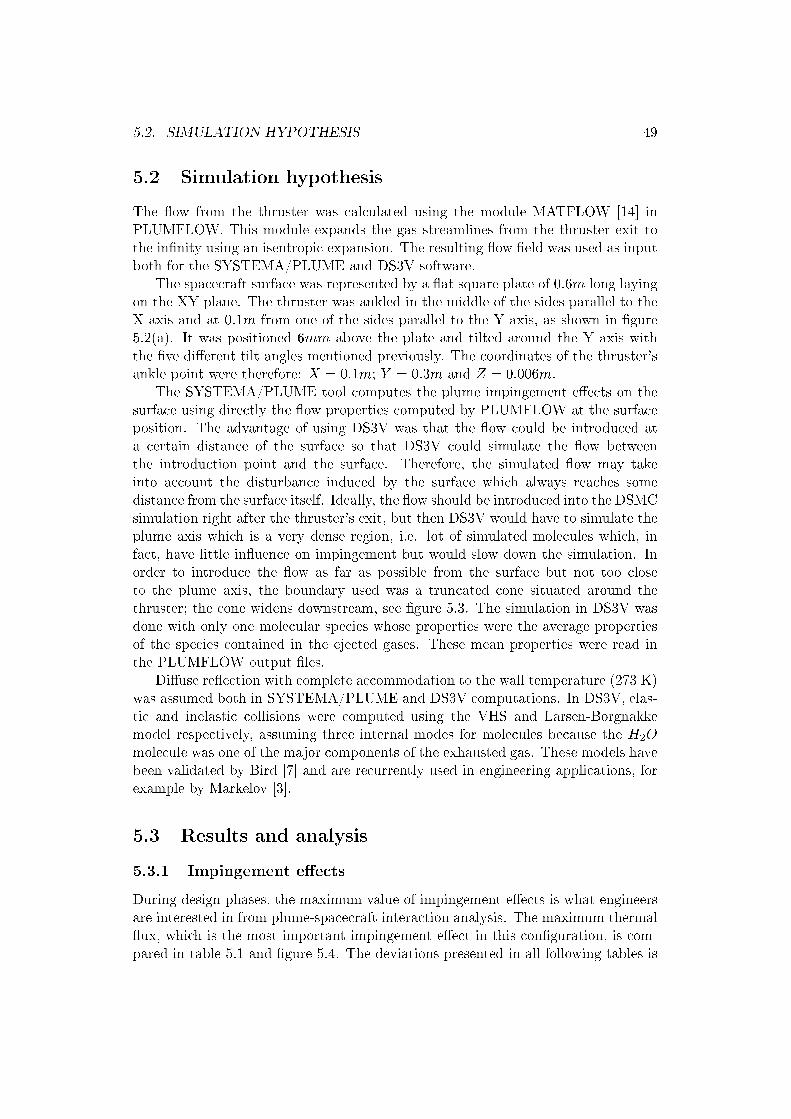
5.2. SIMULATION HYPOTHESIS 49
5.2 Simulation hypothesis
The �ow from the thruster was calculated using the module MATFLOW [14] inPLUMFLOW. This module expands the gas streamlines from the thruster exit tothe in�nity using an isentropic expansion. The resulting �ow �eld was used as inputboth for the SYSTEMA/PLUME and DS3V software.
The spacecraft surface was represented by a �at square plate of 0:6m long layingon the XY plane. The thruster was ankled in the middle of the sides parallel to theX axis and at 0:1m from one of the sides parallel to the Y axis, as shown in �gure5.2(a). It was positioned 6mm above the plate and tilted around the Y axis withthe �ve di�erent tilt angles mentioned previously. The coordinates of the thruster'sankle point were therefore: X = 0:1m; Y = 0:3m and Z = 0:006m.
The SYSTEMA/PLUME tool computes the plume impingement e�ects on thesurface using directly the �ow properties computed by PLUMFLOW at the surfaceposition. The advantage of using DS3V was that the �ow could be introduced ata certain distance of the surface so that DS3V could simulate the �ow betweenthe introduction point and the surface. Therefore, the simulated �ow may takeinto account the disturbance induced by the surface which always reaches somedistance from the surface itself. Ideally, the �ow should be introduced into the DSMCsimulation right after the thruster's exit, but then DS3V would have to simulate theplume axis which is a very dense region, i.e. lot of simulated molecules which, infact, have little in�uence on impingement but would slow down the simulation. Inorder to introduce the �ow as far as possible from the surface but not too closeto the plume axis, the boundary used was a truncated cone situated around thethruster; the cone widens downstream, see �gure 5.3. The simulation in DS3V wasdone with only one molecular species whose properties were the average propertiesof the species contained in the ejected gases. These mean properties were read inthe PLUMFLOW output �les.
Di�use re�ection with complete accommodation to the wall temperature (273 K)was assumed both in SYSTEMA/PLUME and DS3V computations. In DS3V, elas-tic and inelastic collisions were computed using the VHS and Larsen-Borgnakkemodel respectively, assuming three internal modes for molecules because the H2Omolecule was one of the major components of the exhausted gas. These models havebeen validated by Bird [7] and are recurrently used in engineering applications, forexample by Markelov [3].
5.3 Results and analysis
5.3.1 Impingement e�ects
During design phases, the maximum value of impingement e�ects is what engineersare interested in from plume-spacecraft interaction analysis. The maximum thermal�ux, which is the most important impingement e�ect in this con�guration, is com-pared in table 5.1 and �gure 5.4. The deviations presented in all following tables is

50 CHAPTER 5. COMPARISON BETWEEN SYSTEMA/PLUME AND DS3V
(a) Front view
(b) Side view
Figure 5.2: Position of the tilted thruster ankled on a satellited surface
calculated with the DS3V value as reference: xDS3V �xPLUMFLOW
xDS3V.
The �rst important result is that both methods predict the same tendency:the thermal �ux increases when the tilt angle increases. At small tilts, 15 and 20degrees, the error is negligible, while at higher angles, 25, 30 and 35 degrees, theerror is of the order of 10-15% . Nevertheless, 10-15% is a very low and satisfactorydeviation considering that SYSTEMA/PLUME is a very simpli�ed approach whichdi�ers a lot from the DSMC approach. The two methods give very similar thermal�uxes in terms of shape and intensity and this is still true for the �ve tilt angles,

5.3. RESULTS AND ANALYSIS 51
Figure 5.3: Tilted thruster ankled: DS3V simulation boundaries and introductionof the �ow
thruster tilt DS3V SYSTEMA/PLUME Deviation
15° 620 610 -1.6%20° 830 830 0%25° 1130 1260 11.5%30° 1590 1850 16.3%35° 2310 2650 14.7%
Table 5.1: Maximum thermal �ux (W �m�2 � s�1)
compare �gures A.1(a) and A.1(b), A.2(a) and A.2(b), A.3(a) and A.3(b), A.4(a)and A.4(b), A.5(a) and A.5(b). Another important result is that for all tilt angles,except 20°, the distance between the maximum thermal �ux positions predictedwith the two software are smaller than the spatial resolution of the mesh, so it canbe considered that both methods place the maximums at the same position. Oneadditional important thing is that SYSTEMA/PLUME has given worst case resultsfor the thermal �ux; therefore, previous impingement analysis in the back�ow regionhave not underestimated the thermal �ux. All these results are very positive andreinforce our trust in both computational methods.

52 CHAPTER 5. COMPARISON BETWEEN SYSTEMA/PLUME AND DS3V
Figure 5.4: Maximum thermal �ux
thruster tilt DS3V SYSTEMA/PLUME Deviation
15° 5:60 � 1021 4:90 � 1021 13%20° 7:60 � 1021 6:63 � 1021 13%25° 1:10 � 1022 9:51 � 1021 14%30° 1:55 � 1022 1:41 � 1022 9%35° 2:30 � 1022 2:02 � 1022 12%
Table 5.2: Maximum number �ux (molecules �m�2 � s�1)
thruster tilt DS3V SYSTEMA/PLUME Deviation
15° 0.45 0.41 9%20° 0.62 0.58 6%25° 0.83 0.79 5%30° 1.2 1.15 4%35° 1.65 1.72 -4%
Table 5.3: Maximum pressure (Pa)
Figure 5.5 plots the maximum number �ux, at all tilt angles, predicted by bothmethods and table 5.2 gives the deviation with the DS3V value taken as a refer-ence. They both predict an increase of this maximum number �ux as the tilt angleincreases and DS3V gives values 13% higher at all angles except 30 degrees (9% ).
Figure 5.6 plots the maximum pressure which also increases with the angle ac-cording to both methods. Table 5.3 shows that DS3V again predicts higher valuesfor all angles except 35 degrees. As matter of fact, the deviation decreases from

5.3. RESULTS AND ANALYSIS 53
Figure 5.5: Maximum number �ux
Figure 5.6: Maximum pressure
+9% to -4% as the tilt angle increases.Finally, �gure 5.7 plots the maximum shear stress, which also increases with the
angle. However, at all angles, DS3V predicts values around 12% lower, except at 15degrees (3% ), see table 5.4.

54 CHAPTER 5. COMPARISON BETWEEN SYSTEMA/PLUME AND DS3V
thruster tilt DS3V SYSTEMA/PLUME Deviation
15° 0.32 0.33 -3%20° 0.43 0.49 -14%25° 0.63 0.7 -11%30° 0.86 0.97 -13%35° 1.21 1.35 -12%
Table 5.4: Maximum magnitude of shear stress (Pa)
Figure 5.7: Maximum magnitude of shear stress
5.3.2 Plume expansion
In the DS3V calculation, the plume was introduced with a truncated cone, as shownin �gure 5.3. This means that, from the nozzle to the cone surfaces, the plumewas expanded by PLUMFLOW, but from the cone to the spacecraft surface, theexpansion is computed by DS3V, i.e. with the DSMC method. On the contrary, asthe SYSTEMA/PLUME tool computes �ow-surface interaction using the �ow �eldproperties computed by PLUMFLOW at the surface position, the full expansionfrom the nozzle to the surface was done by PLUMFLOW, as shown in �gure 5.8.In other words, even before calculating any �ow-surface interaction, the incident�ow may di�er from one method to the other just due to the di�erent expansionmethods. In this paragraph, comparison between the �ow expanded using DS3Vand PLUMFLOW is presented.
As the goal is to study �ow expansion and not disturbance by the surface, theDS3V expansion was performed exactly as the simulation described in section 5.2with an important di�erence: the solid boundary, i.e. the spacecraft surface, was

5.3. RESULTS AND ANALYSIS 55
(a) Plume expansion in the PLUMFLOW and DS3V computations
(b) DS3V simulation
Figure 5.8: Comparison of plume expansion simulation
removed. In this way, the �ow expands freely from the cone to the surface position,like in the PLUMFLOW computation. Then, by studying the �ow at the formerposition of the spacecraft surface, it could be understood how was the incident �owjust before disturbance due to interaction with the surface. In order to be in the bestconditions to compare this �ow with the �ow used as input by SYSTEMA/PLUMEto compute �ow-surface interaction, a new DS3V simulation was run in the followingway: the plume was introduced a few millimeters before the spacecraft position andthe DS3V computation volume is a parallelepiped just surrounding the spacecraftsurface position, as shown by �gure 5.8(b). Therefore, by looking at the �ow �eldproperties at the spacecraft surface position with the DS3V visualization tools, thetwo expansion approaches could be compared. The comparison was done only with
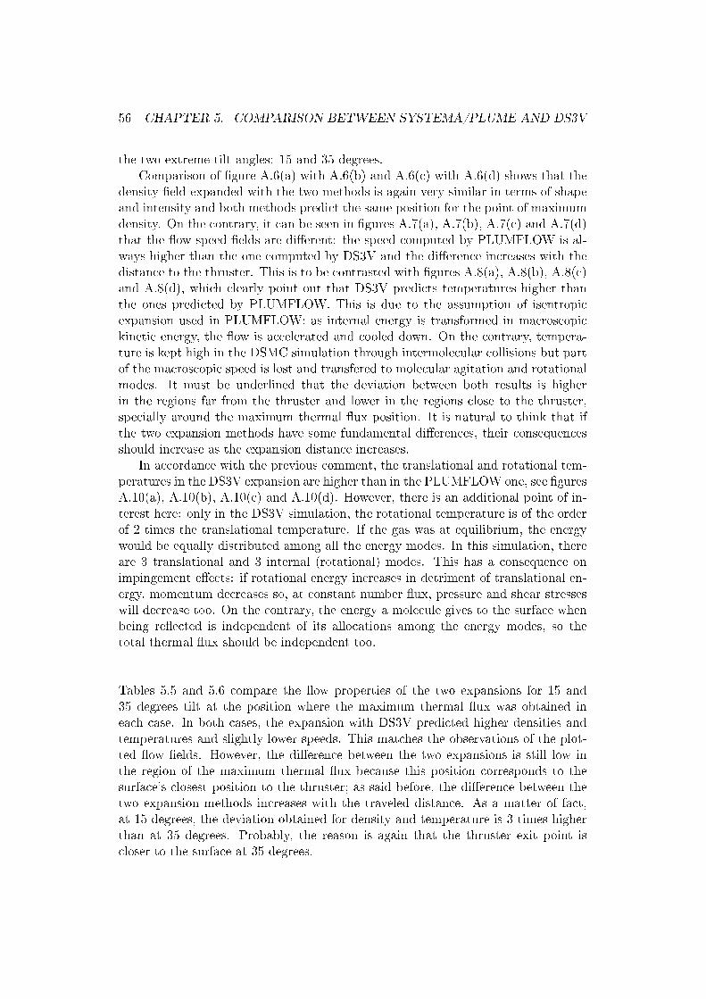
56 CHAPTER 5. COMPARISON BETWEEN SYSTEMA/PLUME AND DS3V
the two extreme tilt angles: 15 and 35 degrees.Comparison of �gure A.6(a) with A.6(b) and A.6(c) with A.6(d) shows that the
density �eld expanded with the two methods is again very similar in terms of shapeand intensity and both methods predict the same position for the point of maximumdensity. On the contrary, it can be seen in �gures A.7(a), A.7(b), A.7(c) and A.7(d)that the �ow speed �elds are di�erent: the speed computed by PLUMFLOW is al-ways higher than the one computed by DS3V and the di�erence increases with thedistance to the thruster. This is to be contrasted with �gures A.8(a), A.8(b), A.8(c)and A.8(d), which clearly point out that DS3V predicts temperatures higher thanthe ones predicted by PLUMFLOW. This is due to the assumption of isentropicexpansion used in PLUMFLOW: as internal energy is transformed in macroscopickinetic energy, the �ow is accelerated and cooled down. On the contrary, tempera-ture is kept high in the DSMC simulation through intermolecular collisions but partof the macroscopic speed is lost and transfered to molecular agitation and rotationalmodes. It must be underlined that the deviation between both results is higherin the regions far from the thruster and lower in the regions close to the thruster,specially around the maximum thermal �ux position. It is natural to think that ifthe two expansion methods have some fundamental di�erences, their consequencesshould increase as the expansion distance increases.
In accordance with the previous comment, the translational and rotational tem-peratures in the DS3V expansion are higher than in the PLUMFLOW one, see �guresA.10(a), A.10(b), A.10(c) and A.10(d). However, there is an additional point of in-terest here: only in the DS3V simulation, the rotational temperature is of the orderof 2 times the translational temperature. If the gas was at equilibrium, the energywould be equally distributed among all the energy modes. In this simulation, thereare 3 translational and 3 internal (rotational) modes. This has a consequence onimpingement e�ects: if rotational energy increases in detriment of translational en-ergy, momentum decreases so, at constant number �ux, pressure and shear stresseswill decrease too. On the contrary, the energy a molecule gives to the surface whenbeing re�ected is independent of its allocations among the energy modes, so thetotal thermal �ux should be independent too.
Tables 5.5 and 5.6 compare the �ow properties of the two expansions for 15 and35 degrees tilt at the position where the maximum thermal �ux was obtained ineach case. In both cases, the expansion with DS3V predicted higher densities andtemperatures and slightly lower speeds. This matches the observations of the plot-ted �ow �elds. However, the di�erence between the two expansions is still low inthe region of the maximum thermal �ux because this position corresponds to thesurface's closest position to the thruster; as said before, the di�erence between thetwo expansion methods increases with the traveled distance. As a matter of fact,at 15 degrees, the deviation obtained for density and temperature is 3 times higherthan at 35 degrees. Probably, the reason is again that the thruster exit point iscloser to the surface at 35 degrees.

5.3. RESULTS AND ANALYSIS 57
Flow property PLUMFLOW DS3V Deviationexpansion expansion
Density (kg=m2) 2:5 � 1018 2:9 � 1018 14%Flow speed (m/s) 2653 2586 -3%
Velocity normal to surface (m/s) 1830 1872 2%Temperature (K) 266 331 20%
Translational temperature (K) 258 204 26%Rotational temperature (K) 273 458 40%
Number �ux (molecules=m2=s) 4:58 � 1021 5:43 � 1021 16%
Table 5.5: Flow properties at the maximum thermal �ux position with a 15° tilt
Flow property PLUMFLOW DS3V Deviation1
expansion expansion
Density (kg=m2) 1:24 � 1019 1:30 � 1019 5%Flow speed (m/s) 2664 2612 -2%
Velocity normal to surface (m/s) 1713 1711 0%Temperature (K) 390 416 6%
Translational temperature (K) 380 286 -33%Rotational temperature (K) 400 546 27%
Number �ux (molecules=m2=s) 2:12 � 1022 2:22 � 1022 5%
Table 5.6: Flow properties at the maximum thermal �ux position with a 35° tilt
In a nutshell, for the con�guration we are studying, even before computing any�ow-surface interaction and the subsequent �ow �eld disturbances, the di�erencein the expansion approach alone leads to deviations from 5 to 20% on �ow proper-ties such as density, temperature and number �ux which have direct in�uence onimpingement e�ects.
5.3.3 DSMC: �ow �eld disturbance
To analyze the �ow �eld disturbance by the presence of the solid surface, it is agood exercise to compare the DS3V simulations with and without solid surface. Thistime, it was more e�cient to visualize the �elds in a XZ plane, i.e. a plane normalto the solid surface. The plane chosen was the plane of symmetry (Y = 0:3m) of thesurface and containing the thruster's axis, see �gure A.11(a). It must be rememberedthat in the simulations with the solid surface, the �ow properties take into accountthe re�ected molecules so it is very di�cult to distinguish between incident andre�ected molecules. For example, in free-molecular regime, intermolecular collisionsare negligible so incident molecules could be treated as a gas and re�ected moleculesas a di�erent gas; however, the program outputs the mean �ow properties in each

58 CHAPTER 5. COMPARISON BETWEEN SYSTEMA/PLUME AND DS3V
cell and this accounts for incident and re�ected molecules.The �rst thing that emerges from comparing �gure A.12(a) with A.12(b) is the
creation of an overpressure on the surface around X = 0:24m (the plate is 0:6mlong). In this region, with the thruster tilted 35°, without surface, the density is ofthe order of 5�10�7kg=m3, while once the surface is immersed in the �ow, the densityincreases to more or less 3:5 � 10�6kg=m3, i.e. 7 times higher. It is natural that thedensity is multiplied by 2 because of the re�ected molecules, but a factor of 7 meansthat a lot of molecules are con�ned in this region through collisions. Comparison of�gures A.11(a) with A.11(b) shows the appearance of an overpressure around thesame region for a 15° tilt as well. However, this time the density is multiplied by afactor of 4 only, instead of 7. The clear reason for this a that the more the thrusteris tilted, the closer it is from the surface. Therefore, the density of the free expanded�ow at the position corresponding to the overpressure in the disturbed �ow case isof the order of 2 � 10�7kg=m3 for 15° and 6 � 10�7kg=m3 for 35°, see �gures A.11(a)and A.12(a). Consequently, there are more collisions in the 35° case and this helpsbuild up a large overpressure.
The supposition about the overpressure being caused by collisions between theincident and re�ected gases is con�rmed by the temperature �elds. Figures A.13(b)and A.14(b) show a sudden increase of temperature up to more than 1000 K thattakes the form of a stream �owing in front of the plate. This hot stream does notappear on the other side of the thruster but most important: the incident �ow has atemperature of no more than 600 K, see �gures A.13(a) and A.14(a) and the di�uselyre�ected gas is fully accommodated to the temperature of the plate (273 K). If therewere no collisions, the temperature would just be the average between these twotemperature, i.e. less than 500 K. It can be concluded that the rise of temperatureup to more than 1000 K is due indeed to collisions that would not occur if therewas no surface. It can also in fact be observed that this hot stream is closer to thesurface when the thruster is tilted 35 degrees than when it is tilted 15 degrees. Thisagain may be attributed to the di�erent position of the thruster: with the large tilt(35°), the re�ected molecules do not need to travel a lot to �nd densities su�cientlyhigh so that the collision probability is high, while with the low tilt (15°), they travelfurther from the surface and closer to the thruster before undergoing intermolecularcollisions. This is proved by the mean collision time �elds. At both tilt angles, themean collision time close to the surface (X = 0:24m) is divided by 10: at 15°, itis of the order of 2 � 10�3sec and 2 � 10�4sec with and without plate respectively(see �gures A.17(a) and A.17(b)), while at 35° it is of the order of 6 � 10�4sec and6 � 10�5sec A.18(a) and A.18(b)). The mean collision time at the most dense pointof the �ve simulations with a surface is plotted in �gure 5.9: it decreases as thethruster comes closer to the surface.
A local Knudsen number was estimated for the �ve tilt angles in the positioncorresponding, for each con�guration, to the maximum thermal �ux and is shownin �gure 5.10. All Knudsen numbers are higher than 0.2, which is the limit of thecontinuum model according to Bird [6], and they are of the order of unity thatindicates that gas in the corresponding region is in the transitional regime and not

5.3. RESULTS AND ANALYSIS 59
Figure 5.9: DS3V simulation: mean collision time in the maximum thermal �uxpoint in function of tilt angle
Figure 5.10: DS3V simulation: local Knudsen number in the maximum thermal �uxpoint in function of tilt angle
in the free-molecular regime yet. The second observation is that there is a cleargap between the two smallest angles, 15° and 20°, and the three largest, 25°, 30°and 35°. This points out that the �ows of the 15° and 20° con�gurations are closerthan the others to the free-molecular regime. In other words, the assumption offree-molecular regime made in SYSTEMA/PLUME is more exact at 15° and 20°tilts than at 25°, 30° and 35°.

60 CHAPTER 5. COMPARISON BETWEEN SYSTEMA/PLUME AND DS3V
These results may explain the impingement e�ects curves: DS3V predicts anumber �ux around 12% higher than SYSTEMA/PLUME at all tilt angles, see table5.2. The pressure is the normal momentum �ux so roughly it is the product of themass �ux (number �ux times the molecular mass) and the mean momentum. Thepressure deviation is clearly reduced in comparison with the number �ux deviationand at 35° the pressure predicted by DS3V is even lower than the one predictedby SYSTEMA/PLUME, see table 5.3. This means that the mean momentum inthe disturbed �ow (DSMC simulation) is lower than the mean momentum beforedisturbance (PLUMFLOW computation) and the tables indicate that this di�erenceis higher at high tilt angles. This can be explained by the fact that the plume �owis stopped by the dense region created by the re�ected molecules. The number �uxin the SYSTEMA/PLUME computation is mainly due to the macroscopic velocityof the gas, while in the DSMC simulation, the number �ux is run, at least partly,by molecular agitation. This explains, too, why DS3V predicts a lower magnitudeof shear stress: in the SYSTEMA/PLUME computation, the shear stress (parallelmomentum �ux) is again run by the parallel macroscopic velocities, while in theDS3V simulation, part of this momentum is transferred to molecular agitation. Asmolecular agitation tends to be isotropic, the parallel momentum �ux decreases.
5.3.4 Conclusion
From a engineering point of view, the most relevant result is that all impingemente�ects predicted by SYSTEMA/PLUME and DS3V have deviations lower than 16%.This is a very satisfactory result because DS3V is a sophisticated and physical ap-proach very di�erent from the simpli�ed and fast SYSTEMA/PLUME method.
A study has been conducted to understand the origin of this di�erence: �rstly,it was observed that the deviation between the �ow properties of the gas expandedwithout surface with PLUMFLOW and DS3V is between 5 and 20%. This deviationincreases as the distance to the thruster increases: therefore, as the thruster is tilteddown (increase of the tilt angle) and brought closer to the surface, the di�erencebetween the impinging �ows at the surface position, before disturbance of the �ow�eld by the surface, decreases.
On the other hand, as the thruster is tilted down, the density of the abovementioned �ow at the surface position increases just because it is closer to thethruster. Consequently, the probability of collision between re�ected and incidentmolecules increases as the thruster is tilted down and the �ow is more disturbedat high (35°) than at low (15°) tilt angles. The estimation of a local Knudsennumber con�rmed that the disturbed gas is in the transitional regime but at smalltilt angles (15° and 20°) it is closer to the free-molecular regime assumed in theSYSTEMA/PLUME approach.
In other words, regarding comparison between the DS3V and SYSTEMA/PLUMEsimulations in the back�ow con�guration, these two phenomena are opposed. The�rst reduces and the second increases the di�erence when the tilt angle increases.

Chapter 6
Use of DS3V for plumeimpingement analysis in anAstrium spacecraft
6.1 Introduction
Plume impingement analysis on the instrument apertures of the Bepi-Colombospacecraft was performed with DS3V. The immediate reason for this was that theinside of the apertures is not in the �eld of view of the thrusters, so the SYS-TEMA/PLUME tool could not be used. An additional reason was that the instru-ments are close to the thrusters so the �ow was suspected to be in the transitionalregime and to be disturbed by solid surfaces. We present brie�y one of this analysisto show an industrial application of the method. Figure 6.1 shows the MercuryTransfer Module (MTM) on top of the Mercury Polar Orbiter (MPO), with hisradiator panel and the apertures for three star trackers. The Bepi-Colombo teamrequested an evaluation of plume-impingement contamination on the star trackerlenses, situated at the bottom of the apertures. The thrusters suspected of contam-inating these lenses are the MTM thrusters 7, 8, 11 and 12, see �gure 6.1, and theMPO thrusters 1, 2, 3 and 4 shown in �gure 6.2. Only the simulation correspondingto the MTM thruster 11 is presented here.
6.2 Hypothesis and simulation method
The simulation starts with the geometry de�nition. In this con�guration, the ra-diator itself was the only structure from the MPO considered as non-super�uousfor the simulation. Therefore, the .STEP (CATIA format) model of the MPO wasimported into RHINOCEROS and everything, except the radiator panel, was sup-pressed. Also, the geometrical details of the radiator that were supposed to haveno in�uence in the results but would complicate the 3D model were eliminated.The goal was to obtain the simplest but realistic model in order to mesh it easily.
61
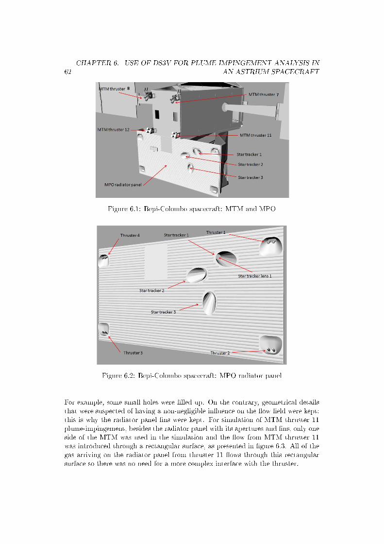
62CHAPTER 6. USE OF DS3V FOR PLUME IMPINGEMENT ANALYSIS IN
AN ASTRIUM SPACECRAFT
Figure 6.1: Bepi-Colombo spacecraft: MTM and MPO
Figure 6.2: Bepi-Colombo spacecraft: MPO radiator panel
For example, some small holes were �lled up. On the contrary, geometrical detailsthat were suspected of having a non-negligible in�uence on the �ow �eld were kept:this is why the radiator panel �ns were kept. For simulation of MTM thruster 11plume-impingement, besides the radiator panel with its apertures and �ns, only oneside of the MTM was used in the simulation and the �ow from MTM thruster 11was introduced through a rectangular surface, as presented in �gure 6.3. All of thegas arriving on the radiator panel from thruster 11 �ows through this rectangularsurface so there was no need for a more complex interface with the thruster.
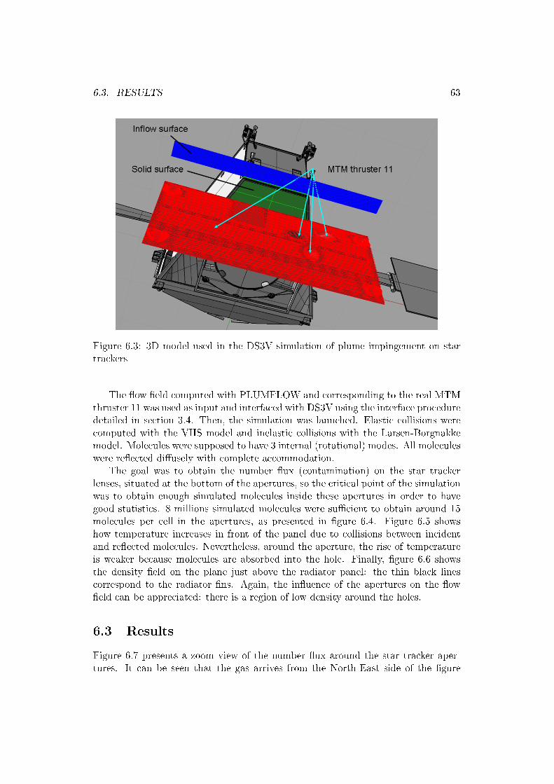
6.3. RESULTS 63
Figure 6.3: 3D model used in the DS3V simulation of plume impingement on startrackers
The �ow �eld computed with PLUMFLOW and corresponding to the real MTMthruster 11 was used as input and interfaced with DS3V using the interface proceduredetailed in section 3.4. Then, the simulation was launched. Elastic collisions werecomputed with the VHS model and inelastic collisions with the Larsen-Borgnakkemodel. Molecules were supposed to have 3 internal (rotational) modes. All moleculeswere re�ected di�usely with complete accommodation.
The goal was to obtain the number �ux (contamination) on the star trackerlenses, situated at the bottom of the apertures, so the critical point of the simulationwas to obtain enough simulated molecules inside these apertures in order to havegood statistics. 8 millions simulated molecules were su�cient to obtain around 15molecules per cell in the apertures, as presented in �gure 6.4. Figure 6.5 showshow temperature increases in front of the panel due to collisions between incidentand re�ected molecules. Nevertheless, around the aperture, the rise of temperatureis weaker because molecules are absorbed into the hole. Finally, �gure 6.6 showsthe density �eld on the plane just above the radiator panel: the thin black linescorrespond to the radiator �ns. Again, the in�uence of the apertures on the �ow�eld can be appreciated: there is a region of low density around the holes.
6.3 Results
Figure 6.7 presents a zoom view of the number �ux around the star tracker aper-tures. It can be seen that the gas arrives from the North-East side of the �gure
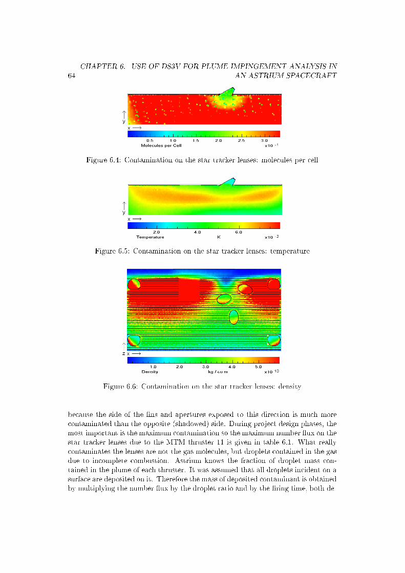
64CHAPTER 6. USE OF DS3V FOR PLUME IMPINGEMENT ANALYSIS IN
AN ASTRIUM SPACECRAFT
Figure 6.4: Contamination on the star tracker lenses: molecules per cell
Figure 6.5: Contamination on the star tracker lenses: temperature
Figure 6.6: Contamination on the star tracker lenses: density
because the side of the �ns and apertures exposed to this direction is much morecontaminated than the opposite (shadowed) side. During project design phases, themost important is the maximum contamination so the maximum number �ux on thestar tracker lenses due to the MTM thruster 11 is given in table 6.1. What reallycontaminates the lenses are not the gas molecules, but droplets contained in the gasdue to incomplete combustion. Astrium knows the fraction of droplet mass con-tained in the plume of each thruster. It was assumed that all droplets incident on asurface are deposited on it. Therefore the mass of deposited contaminant is obtainedby multiplying the number �ux by the droplet ratio and by the �ring time, both de-

6.3. RESULTS 65
pending on the thruster. Finally, the maximum thickness of deposited contaminantgiven in table 6.1 was obtained by summing the contribution of all thrusters. Themain contaminant on the three star trackers was MTM thruster 7. This is partlybecause the apertures are not in the back, but in the front �eld of the thruster andgas molecules fall inside just by traveling directly from the thruster with a parabolictrajectory; they do not need to undergo surface re�ections to reach the apertures.Another reason is that MTM thruster 7 has a high droplet ratio (1.84% ) comparedto the other thrusters, for example MTM thruster 11 (1.43% ). It also �res longer(3846 sec.) than the MPO thrusters (3122 sec.). Thruster 8 has exactly the samecharacteristics as MTM thruster 7 but it is positioned a lot further from the startracker apertures.
Figure 6.7: Contamination on the star tracker lenses due to thruster 11: number�ux
Star tracker lens Maximum Number Flux Maximum Thickness of Deposited(molecules �m�2 � s�1) Contaminant from all Thrusters (�m)
1 1:63 � 1019 6.22 1:97 � 1018 0.33 3:58 � 1018 0.4
Table 6.1: Contaminant deposition on the star tracker lenses


Chapter 7
Conclusion
Bird's DMSC code DS3V was interfaced with Astrium's tool PLUMFLOW, whichcomputes the thruster's plume, and with the commercial 3D modeler RHINOCEROSin order to perform accurate analysis of plume impingement on spacecraft. Thishas already allowed the Space Physics section of the Modeling, Tools and Simula-tion department in Astrium to analyze complex geometry con�gurations in di�erentspacecraft, such as Bepi-Colombo, with a proved simulation method. Moreover,each simulation lasts from a few hours to a few days maximum: this permits themethod to be used with �exibility during design phase and iterate e�ciently withother departments.
The Space Physics section also employs the SYSTEMA/PLUME tool for plume-spacecraft interaction analysis. It is based on a simpli�ed and fast approach whichis supposed to be accurate when the �ow is in the free-molecular regime and the�ow �eld disturbance by solid surfaces is negligible. On the contrary, this approachmay induce error in the transitional regime. In order to quantify this error, SYS-TEMA/PLUME results were compared with DS3V results in a typical Astriumcon�guration where the �ow is in the transitional regime: a thruster's back�owimpingement in the thruster's vicinity. The results were promising: the deviationbetween the plume impingement e�ects predicted by both methods was always lessthan 15% .
However, this deviation might change depending on the con�guration. It issupposed that deviation should decrease as the �ow �eld becomes more rare�ed.Then we think that it is necessary to continue the study and compare both simulationmethods in other con�gurations. The goal is to have a very precise idea of howaccurate is SYSTEMA/PLUME in all typical Astrium con�gurations so one canchoose which simulation method to use.
Also important is to improve PLUMFLOW in order to have less di�erencesbetween PLUMFLOW and DS3V expansions. DS3V can be used to assess theaccuracy of PLUMFLOW.
67


Appendix A
69

70 APPENDIX A.
(a) SYSTEMA/PLUME results
(b) DS3V results
Figure A.1: Comparison of the thermal �ux given by PLUME and DS3V for a tiltof 15 degrees

71
(a) SYSTEMA/PLUME results
(b) DS3V results
Figure A.2: Comparison of the thermal �ux given by PLUME and DS3V for a tiltof 20 degrees

72 APPENDIX A.
(a) SYSTEMA/PLUME results
(b) DS3V results
Figure A.3: Comparison of the thermal �ux given by PLUME and DS3V for a tiltof 25 degrees

73
(a) SYSTEMA/PLUME results
(b) DS3V results
Figure A.4: Comparison of the thermal �ux given by PLUME and DS3V for a tiltof 30 degrees

74 APPENDIX A.
(a) SYSTEMA/PLUME results
(b) DS3V results
Figure A.5: Comparison of the thermal �ux given by PLUME and DS3V for a tiltof 35 degrees

75
(a) 15° tilt: PLUMFLOW expansion (b) 15° tilt: DS3V expansion
(c) 35° tilt: PLUMFLOW expansion (d) 35° tilt: DS3V expansion
Figure A.6: The density �eld at the surface position in a free expansion withoutsolid surface

76 APPENDIX A.
(a) 15° tilt: PLUMFLOW expansion (b) 15° tilt: DS3V expansion
(c) 35° tilt: PLUMFLOW expansion (d) 35° tilt: DS3V expansion
Figure A.7: The �ow speed �eld at the surface position in a free expansion withoutsolid surface

77
(a) 15° tilt: PLUMFLOW expansion (b) 15° tilt: DS3V expansion
(c) 35° tilt: PLUMFLOW expansion (d) 35° tilt: DS3V expansion
Figure A.8: The temperature �eld at the surface position in a free expansion withoutsolid surface

78 APPENDIX A.
(a) 15° tilt: PLUMFLOW expansion (b) 15° tilt: DS3V expansion
(c) 35° tilt: PLUMFLOW expansion (d) 35° tilt: DS3V expansion
Figure A.9: The velocity normal to the surface �eld at the surface position in a freeexpansion without solid surface

79
(a) Translational temperature at 35° tilt:PLUMFLOW expansion
(b) Translational temperature at 35° tilt:DS3V expansion
(c) Rotational temperature at 35° tilt: PLUM-FLOW expansion
(d) Rotational temperature at 35° tilt: DS3Vexpansion
Figure A.10: The translational and rotational temperature �elds at the surfaceposition in a free expansion without solid surface

80 APPENDIX A.
(a) Free expansion (b) Flow disturbed by the surface
Figure A.11: DS3V simulation 15°: density �eld of the free expanded �ow and the�ow disturbed by the solid surface
(a) Free expansion (b) Flow disturbed by the surface
Figure A.12: DS3V simulation 35°: density �eld of the free expanded �ow and the�ow disturbed by the solid surface
(a) Free expansion (b) Flow disturbed by the surface
Figure A.13: DS3V simulation 15°: temperature �eld of the free expanded �ow andthe �ow disturbed by the solid surface
(a) Free expansion (b) Flow disturbed by the surface
Figure A.14: DS3V simulation 35°: temperature �eld of the free expanded �ow andthe �ow disturbed by the solid surface

81
(a) Free expansion (b) Flow disturbed by the surface
(c) Free expansion (d) Flow disturbed by the surface
Figure A.15: DS3V simulation 15°: translational and rotational temperatures �eldsof the free expanded �ow and the �ow disturbed by the solid surface
(a) Free expansion: translational tempera-ture
(b) Flow disturbed by the surface: transla-tional temperature
(c) Free expansion: rotational temperature (d) Flow disturbed by the surface: rotationaltemperature
Figure A.16: DS3V simulation 35°: translational and rotational temperatures �eldsof the free expanded �ow and the �ow disturbed by the solid surface

82 APPENDIX A.
(a) Free expansion (b) Flow disturbed by the surface
Figure A.17: DS3V simulation 15°: mean collision time of the free expanded �owand the �ow disturbed by the solid surface
(a) Free expansion (b) Flow disturbed by the surface
Figure A.18: DS3V simulation 35°: mean collision time of the free expanded �owand the �ow disturbed by the solid surface
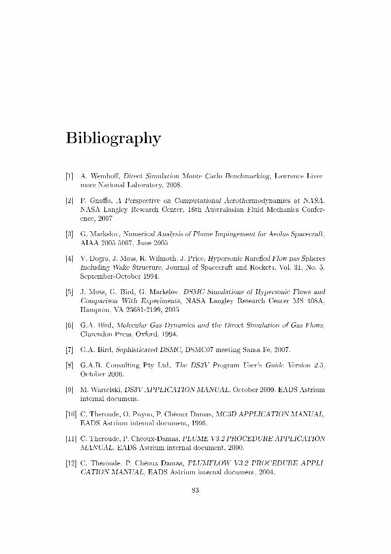
Bibliography
[1] A. Wemho�, Direct Simulation Monte Carlo Benchmarking, Lawrence Liver-more National Laboratory, 2008.
[2] P. Gno�o, A Perspective on Computational Aerothermodynamics at NASA,NASA Langley Research Center, 16th Australasian Fluid Mechanics Confer-ence, 2007
[3] G. Markelov, Numerical Analysis of Plume Impingement for Aeolus Spacecraft,AIAA 2005-5067, June 2005
[4] V. Dogra, J. Moss, R. Wilmoth, J. Price, Hypersonic Rare�ed Flow pas SpheresIncluding Wake Structure, Journal of Spacecraft and Rockets, Vol. 31, No. 5,September-October 1994.
[5] J. Moss, G. Bird, G. Markelov, DSMC Simulations of Hypersonic Flows andComparison With Experiments, NASA Langley Research Center MS 408A,Hampton, VA 23681-2199, 2005
[6] G.A. Bird, Molecular Gas Dynamics and the Direct Simulation of Gas Flows,Clarendon Press, Oxford, 1994.
[7] G.A. Bird, Sophisticated DSMC, DSMC07 meeting Santa Fe, 2007.
[8] G.A.B. Consulting Pty Ltd, The DS3V Program User's Guide Version 2.5,October 2006.
[9] M. Wartelski, DS3V APPLICATION MANUAL, October 2009, EADS Astriuminternal document.
[10] C. Theroude, O. Puyoo, P. Chèoux-Damas, MC3D APPLICATION MANUAL,EADS Astrium internal document, 1996.
[11] C. Theroude, P. Chèoux-Damas, PLUME V3.2 PROCEDURE APPLICATIONMANUAL, EADS Astrium internal document, 2000.
[12] C. Theroude, P. Chèoux-Damas, PLUMFLOW V3.2 PROCEDURE APPLI-CATION MANUAL, EADS Astrium internal document, 2004.
83

84 BIBLIOGRAPHY
[13] C. Theroude, P. Chèoux-Damas, MATPLIMP V3.2 APPLICATION MAN-UAL, EADS Astrium internal document, 2002.
[14] C. Theroude, P. Chèoux-Damas, MATFLOW V3.2 MODULE APPLICATIONMANUAL, EADS Astrium internal document, 2004