Simulation of Patients Routing from an Emergency ... · Simulation of Patients Routing from an...
60
Simulation of Patients Routing from an Emergency Department to Internal Wards in Rambam Hospital Project in “System Analysis and Design” course November 24, 2008 Yulia Tseytlin, Asaf Zviran Course Lecturer: Prof. Michal Penn Academic Advisor: Prof. Avishai Mandelbaum Industry Advisor: Mira Shiloach, Nursing Manager of Internal Wards, Rambam The Faculty of Industrial Engineering and Management Technion - Israel Institute of Technology 1
Transcript of Simulation of Patients Routing from an Emergency ... · Simulation of Patients Routing from an...

Simulation of Patients Routing from an
Emergency Department to Internal Wards
in Rambam Hospital
Project in “System Analysis and Design” course
November 24, 2008
Yulia Tseytlin, Asaf Zviran
Course Lecturer: Prof. Michal Penn
Academic Advisor: Prof. Avishai Mandelbaum
Industry Advisor: Mira Shiloach, Nursing Manager
of Internal Wards, Rambam
The Faculty of Industrial Engineering and Management
Technion - Israel Institute of Technology
1

Acknowledgements
This research project is a requirement of the graduate course “System Analysis and
Design”, in the Faculty of Industrial Engineering and Management, Technion. We wish
to thank the course instructor, Prof. Michal Penn, for her valuable guidance and support
throughout every stage of the work.
The project was carried out under the supervision of Prof. Avishai Mandelbaum. We
would like to express him our gratitude for his valuable help and advice, for sharing his
vast knowledge and experience.
We wish to thank our Rambam advisor Mira Shiloach, nursing manager of the Emer-
gency Department and Internal Wards, for her willingness to assist and share, for her
time and help, and for acquainting us with the key people in the hospital. Our deepest
gratitude goes to Rambam management, especially to Dr. Yaron Bar-El, medical opera-
tions director, who opened for us all the doors that had to be opened. We are thankful
to the staff of the Emergency Department for making our visits to the hospital exciting,
for allowing us to interview them and for sharing their knowledge and thoughts.
Finally, special thanks go to Yariv Marmor for his invaluable help in data analysis.
2

Research Definition and Summary
Problem Definition
The project focuses on the process of patients routing from an Emergency Department
(ED) to four Internal Wards (IW) in Rambam Hospital. The decision in which ward to
hospitalize a patient is made on the basis of a computer program, referred to at the hospi-
tal as the “Justice Table”, which, as its name suggests, is aimed to produce fair allocation
of patients to the wards. But several aspects, like patient Lengths of Stay (LOS) in the
wards, are not taken into account in the Justice Table and that undermines its fairness
and makes us search for other possible routing policies. Besides, waiting times in the
ED from the hospitalization decision till admission to the ward might be quite long, thus
causing overcrowding in the ED and lowering the quality of treatment.
Research Goal
We aim to examine various routing policies in the sense of fairness of the allocation
and operational performance, while accounting for availability of information. We strive
to find out what routing algorithm might be “optimal”: both fair and best-performing.
For that purpose we wish to create a computer simulation model of the process of pa-
tients routing from the ED to the IW in Rambam Hospital, define various fairness and
performance measures to form a single integrated criterion of quality, propose and evalu-
ate various routing policies according to this criterion.
Work Methods
Prior to building a simulation tool, we studied the routing process, both from previ-
ous studies on the subject and from visiting the hospital - conducting observations and
interviews. Later we collected and analyzed empiric quantitative data required for esti-
mating the simulation parameters. Then a generic computer simulation model was built
in Matlab software, matched and validated versus the empiric data. In order to define
an integrated criterion of quality we characterized various fairness criteria (from points-
of-view of wards’ medical and nursing staff, management and patients) and operational
performance measures (average waiting time in the ED before patients’ transfer to the
IW). From there different routing algorithms were deduced, while accounting for avail-
ability of information in the system, and implemented in the simulation. We evaluated
the algorithms according to the optimality criteria and compared them.
3
Results Summary
We propose several routing algorithms, some very intuitive and simple, and some
more complex. The former include Round Robin algorithms - routing according to a
certain predefined order. From the latter we distinguish the occupancy balancing method,
which aims to balance ward occupancies in each moment of routing. It shows very good
performance: low and balanced occupancy rates, short waiting and sojourn times in the
system. However, the occupancy balancing algorithm sends more patients to the fastest
ward which is unfair to its staff. The flow balancing method aims to keep an equal
number of patients per bed per year - it addresses another fairness criterion but causes
longer waits. By adjusting the weights in the weighted algorithm, which combines these
two methods, we can achieve both fairness for the staff and good operational performance.
Additionally, we implement the occupancy balancing method in partial information access
systems (one update per day) with almost no worsening in performance. We conclude that
the proposed weighted algorithm achieves the best performance (in terms of fairness and
minimal weighting time) and may be implemented in partial information access systems,
which is easier to design and implement in hospital settings.
4

Contents
1 Introduction 8
1.1 Rambam Hospital, ED and IW . . . . . . . . . . . . . . . . . . . . . . . . 9
1.2 Routing Process and Justice Table . . . . . . . . . . . . . . . . . . . . . . 10
1.3 Literature Review . . . . . . . . . . . . . . . . . . . . . . . . . . . . . . . . 13
2 Model Description 15
2.1 Data Collection and Analysis . . . . . . . . . . . . . . . . . . . . . . . . . 16
3 Simulation Description 19
3.1 Modules and Design . . . . . . . . . . . . . . . . . . . . . . . . . . . . . . 19
3.2 Model Implementation . . . . . . . . . . . . . . . . . . . . . . . . . . . . . 23
3.3 Validation Versus Empirical Data . . . . . . . . . . . . . . . . . . . . . . . 25
4 Algorithms 29
4.1 Performance Criteria (qualitative) . . . . . . . . . . . . . . . . . . . . . . . 29
4.2 Performance Criteria (quantitative) . . . . . . . . . . . . . . . . . . . . . . 31
4.3 Algorithms description and results . . . . . . . . . . . . . . . . . . . . . . . 33
4.3.1 No Access to System Information . . . . . . . . . . . . . . . . . . . 33
4.3.2 Full Information . . . . . . . . . . . . . . . . . . . . . . . . . . . . . 38
4.3.3 Partial Information . . . . . . . . . . . . . . . . . . . . . . . . . . . 42
4.3.4 Weighted Algorithm . . . . . . . . . . . . . . . . . . . . . . . . . . 44
4.4 Algorithm Comparison . . . . . . . . . . . . . . . . . . . . . . . . . . . . . 47
5 Summary and Conclusions 48
5
6 Limitations and Ideas for Future Research 50
A Routing Process Flow Charts 56
B Arrivals and LOS Empirical Data Analysis 59
List of Figures
1.1 Integrated (Activities - Resources) Flow Chart . . . . . . . . . . . . . . . . 12
2.1 Simulation Model . . . . . . . . . . . . . . . . . . . . . . . . . . . . . . . . 15
2.2 Arrivals to Wards . . . . . . . . . . . . . . . . . . . . . . . . . . . . . . . . 16
3.1 Simulation Infrastructure . . . . . . . . . . . . . . . . . . . . . . . . . . . 20
3.2 System . . . . . . . . . . . . . . . . . . . . . . . . . . . . . . . . . . . . . . 24
3.3 Arrivals to Wards: Validation . . . . . . . . . . . . . . . . . . . . . . . . . 26
3.4 Entrance and Departure Inter-Arrival Times Histograms . . . . . . . . . . 26
3.5 LOS Distribution Validation (LOS in days) . . . . . . . . . . . . . . . . . . 27
3.6 Occupancy (# of occupied beds) Rate Validation . . . . . . . . . . . . . . 28
4.1 RR 1111 Occupancy Rate . . . . . . . . . . . . . . . . . . . . . . . . . . . 34
4.2 RR 1111 Occupancy Standard Deviation . . . . . . . . . . . . . . . . . . . 35
4.3 RR 1111 Sojourn Time . . . . . . . . . . . . . . . . . . . . . . . . . . . . . 35
4.4 RR 3233 Occupancy Rate . . . . . . . . . . . . . . . . . . . . . . . . . . . 36
4.5 RR 3233 Occupancy Standard Deviation . . . . . . . . . . . . . . . . . . . 37
4.6 RR 3233 Sojourn Time . . . . . . . . . . . . . . . . . . . . . . . . . . . . . 37
4.7 IB Occupancy Rate . . . . . . . . . . . . . . . . . . . . . . . . . . . . . . . 38
4.8 IB Occupancy Standard Deviation . . . . . . . . . . . . . . . . . . . . . . . 39
6

4.9 Min-stdev Occupancy Rate . . . . . . . . . . . . . . . . . . . . . . . . . . . 40
4.10 Min-stdev Occupancy Standard Deviation . . . . . . . . . . . . . . . . . . 41
4.11 Min-stdev Sojourn Time . . . . . . . . . . . . . . . . . . . . . . . . . . . . 41
4.12 Partial-Information Occupancy Rate . . . . . . . . . . . . . . . . . . . . . 43
4.13 Partial-Information Occupancy Standard Deviation . . . . . . . . . . . . . 44
4.14 Partial-Information Sojourn Time . . . . . . . . . . . . . . . . . . . . . . . 44
4.15 Weighted Occupancy Rate . . . . . . . . . . . . . . . . . . . . . . . . . . . 46
4.16 Weighted Occupancy Standard Deviation . . . . . . . . . . . . . . . . . . . 47
4.17 Summary Table . . . . . . . . . . . . . . . . . . . . . . . . . . . . . . . . . 48
A.1 Activities Flow Chart . . . . . . . . . . . . . . . . . . . . . . . . . . . . . . 56
A.2 Resources Flow Chart . . . . . . . . . . . . . . . . . . . . . . . . . . . . . 57
A.3 Information Flow Chart . . . . . . . . . . . . . . . . . . . . . . . . . . . . 58
B.1 Compatibility of Arrivals Distribution to Poisson - Sunday . . . . . . . . . 59
B.2 Compatibility of LOS distribution to Log-Normal - Ward A . . . . . . . . 60
List of Tables
2.1 Standard and Maximal Capacity (# beds) of the Internal Wards . . . . . . 17
2.2 LOS (days) in the Internal Wards . . . . . . . . . . . . . . . . . . . . . . . 17
7

1 Introduction
Health care systems in general, and hospitals in particular, represent a very important
part of the service sector. Over the years, hospitals have been successful in using medi-
cal and technical innovations to deliver more effective clinical treatments while reducing
patients’ time spent in the hospital. However, hospitals are typically rife with inefficien-
cies and delays, thus present a propitious ground for many research projects in numerous
science fields, and in the Operations Research field in particular.
A hospital is an institution for health care, which is able to provide long-term patient
stays. Hospitals include numerous medical units specializing each in a different area of
medicine, such as internal, surgery, intensive care, obstetrics, and so forth. In most of the
large hospitals there are several similar medical units operating in parallel. In our project
we focus on an Emergency Department (ED) and its interface with four Internal Wards
(IW) in Rambam Hospital.
The ED deals with immediate threats to health and provides emergency medical ser-
vices. Thus the proper functioning of the ED is of utter importance, and its overcrowding
can cause inability to admit new patients and ambulances diversion. A patient arriving
to the ED undergoes registration, diagnostic testing, basic treatment, and then is either
dismissed or admitted to stay, the latter if doctors decide on hospitalization, in which
case the patient is transferred to the appropriate medical unit. In our project we focus on
admitted patients, specifically on the process from the decision of hospitalization till ad-
mission to the IW. The project continues, in some aspects, the IE undergraduate project
of K. Elkin and N. Rozenberg [8] that was performed in Rambam hospital in 2006-2007.
Elkin and Rozenberg studied meticulously the routing process, and their work provided
us with much of the necessary background.
The main goals of our project are to create a computer simulation model of the pro-
cess of patients routing from the ED to the IW in Rambam Hospital and, with its help,
to examine various routing policies in order to propose an “optimal” one. The project
stages included: (1) Comprehensive study of the process both from [8] and from visiting
Rambam, conducting observations and interviews; (2) Collecting and analyzing the quan-
titative data necessary for the simulation parameters; (3) Building a computer simulation
model in Matlab, matching and validating it versus the empirical data; (4) Characterizing
various fairness criteria (from points-of-view of wards’ medical and nursing staff, manage-
ment and patients) and operational performance measures (average waiting time in the
ED before the transfer), in order to define an “optimal” routing policy; (5) Deducing dif-
ferent routing policies, while accounting for availability of information in the system, and
8

implementing them in the simulation; (6) Evaluating the algorithms versus the optimality
criteria and comparing them.
This project report is structured as follows: first we provide a background on the
hospital, the medical units in question, the process of interest and the problems involved,
and survey the relevant literature. In the next section we describe the model which lays at
the basis of the simulation and the empirical data used to build it. In Section 3 we present
the simulation model: its design, documentation and validation. Then fairness criteria,
routing algorithms and results achieved in the simulation are described. We summarize
these results in Section 5, and present the limitations of the project and ideas for further
research in concluding Section 6.
Remark: We wish to mention that, in the course of the work on the project, the
ED was moved to a temporary location (the Basement) where it will remain for a couple
of years, while its permanent location is renovated and expanded. Most of the data was
collected on the period prior to the move, but, as far as we are concerned, are relevant to
the current situation.
1.1 Rambam Hospital, ED and IW
Rambam Health Care Campus established in 1938, is the largest medical center in
Northern Israel, which serves over two million citizens. With 1000 beds in 36 depart-
ments, 45 medical units, 9 institutes, 6 laboratories and 30 administrative and main-
tenance departments, Rambam delivers the full spectrum of healthcare services. Some
75,000 people are hospitalized at Rambam each year, with another 500,000 treated in
its outpatient clinics and medical institutes. Among the variety of its medical sections,
Rambam has a large Department of Emergency Medicine with a capacity of 40 beds; and
five Internal Wards, denoted from A to E.
The ED receives and treats more than 200 patients daily, and is divided into two
major subunits: Internal and Trauma (surgical and orthopedic patients), each of those is
divided into “walking” and “lying” subunits, according to the state of patients treated
there. An internal patient, whom the ED decides to hospitalize, is directed to one of the
five Internal Wards according to a certain routing policy - and this process is precisely
our focus of interest.
Internal Medicine Departments are responsible for the treatment of a wide range of
internal disorders, providing inpatient medical care to thousands of patients each year.
9

Wards A-D are more or less the same in their medical capabilities - each can treat multiple
types of patients. Ward E, on the other hand, treats only “walking” patients, and the
routing process from the ED to it differs from the one to the other wards (see description
below). In our project we concentrate on the routing process to wards A-D only.
1.2 Routing Process and Justice Table
A patient, whom the ED physician in charge decides to hospitalize in the IW, is
assigned to one of the five wards in the following way: If this is an “independent” walking
patient, usually he or she is assigned to Ward E, otherwise the routing decision is made
on the basis of a computer program, referred to at the hospital as the “Justice Table”.
The program receives a patient’s category (described below) as an input parameter and
returns a ward for the patient (A-D) as an output. As its name suggests, the algorithm is
supposed to do justice with the wards: to make the patients’ allocation to the wards fair.
Below we describe briefly the history of the Justice Table from its inception to nowadays.
Before 1997: Patients’ allocation was decided according to a fixed “table of duty”
of the wards (every day another ward was on duty and had to accommodate all the
incoming patients), but it was subjugated to the wards’ approval - each ward had the
authority to refuse to admit a patient. Consequently, waiting times in the ED until
transfer to the IW were extremely long - 10.5 hours on the average, with 12% of the
patients forced to wait more than 24 hours (!) [16]. This caused a heavy overload on
the ED and hence department’s malfunctioning. In 1995, as part of an overall Rambam
quality program, a dedicated team for improving processes in the ED was founded - its
goal was, in particular, to reduce the ED-IW waiting times. The team [16] proposed a
change in the existing routing policy: a patient’s placement would be determined by an
algorithm named the “Justice Table”, and the authority for patients’ routing would be
taken away from the wards.
Short description of the ‘Justice Table” algorithm: The purpose of the “Justice
Table” was to balance the load among the wards. It was decided to classify patients into
three categories: ventilated - patients that required artificial respiration, special care -
patients whose rate on the Norton scale (a table used to predict if a patient might develop
a pressure ulceration) was below 14, and regular - all other patients. Lengths Of Stay
(LOS) and complexity of treatment varied significantly among those categories, which is
why the Table directed each category independently in order to ensure fair allocation.
For each patients’ category there were “fixed turns” among the wards, namely each ward
received one patient in its turn. In addition to a patient’s classification, the algorithm
10

took into account the size of each ward, but only its static capacity and not the actual
occupancy at the time the routing decision was made.
The current situation: The results of implementing the new routing policy were
very impressive - average waiting time from the decision about hospitalization till moving
the patient to a ward was reduced to 66 minutes [16]. In addition, a significant improve-
ment in other ED processes was measured as well (due to an overload reduction), along
with a higher IW efficiency (more admissions, shorter LOS). But in 2004, the use of the
Justice Table was discontinued, due to software changes in Rambam.
In 2006, adapted to the new software, the Justice Table was reinstated with minor
changes, but its influence grew smaller, as the medical staff had become used to making
placement decisions without the Table. Thus, in the observations that [8] conducted, it
turned out that a significant number of the patients transferred from the ED to the IW
were not routed via the Justice Table.
The process of patients routing: One can fully appreciate the complexity of the
process in the Integrated (Activities - Resources) Flow Chart (see Figure 1.1) and other
flow charts (see Appendix A). We provide here a short description: After a physician in
charge of the ED decides to hospitalize a patient in the IW, a receptionist of the ED runs
the Justice Table. She transfers the output of the Table to the nurse in charge of the
ED, who starts a negotiation process with the chosen ward. If the ward refuses to admit
the patient (for reasons of overloading usually), the two sides appeal to a General Nurse
(appointed by the hospital administration, who is authorized to approve the so-called
“skipping” - allow a ward to skip its turn). If skipping is granted, the secretary runs the
Justice Table again, and the process repeats itself until some ward agrees (or is forced)
to accept the patient.
The next stage of the negotiations is agreeing upon the time at which the patient will
be transferred to his ward. The interests are conflicting: the ED seeks to discharge the
patient as soon as possible in order to be able to accept new ones, and the IW’s wish to
have the move carried out at a time convenient for them. From conversations with nurses
from both sides we learn that, when deciding a patient’s transferral time, the main issue
taken into account (assuming there is an available bed in the ward) is nurses’ and doctors’
availability (they might be unavailable because of treating other patients, shifts changing
or meals, various staff meetings or resuscitation). Another parameter is availability of
necessary equipment and other logistic considerations: for example, preparation for a
“complicated” patient who requires special bed/equipment, or placement near nursing
station, takes a longer time.
11

Figure 1.1: Integrated (Activities - Resources) Flow Chart
ED physician
IW nurse, Help force
Stretcher Bearer
IW nurse in charge
General NurseReceptionistED nurse in
chargeIW
physician
Hospitaliza-tion
decision
Patient allocation request
Transferal time
decision
Patient’s status
updating
Coordination with the IW
Running the Justice Table
Request skipping?
Approve skipping?
Initial measurements
collection
Patient’s transferal
Availability check
Bed preparation
Initial medical check
Yes
No
YesNo
Resource Queue - Synchronization Queue -
Availability check
Ventilated patient
- Ending point of simultaneous processes
Transferal time
decision
“Walking patient” Ward E
Ward E
Ward E
Problems in the current process: The first problem is that, prior to their hospi-
talization, patients often must wait a long time in the ED until they are moved to their
IW. From 182 observations that [8] conducted in May 2007, one sees that the average
waiting time from a decision of a patient’s hospitalization till his admission in the IW
is 97 minutes on average. The longest waiting time is for admission in Ward B (112
minutes), waiting times for admission in the other wards are more or less similar (around
90 minutes). During our visit in the ED we received an impression (from conversation
with the nurse in charge) that the waiting times are longer. We learnt that there exists
an agreement obliging the wards to admit patients within four hours from the decision to
hospitalize them, but in certain cases it takes even longer. Exact data on those waiting
times are not kept in Rambam information systems, thus we could not learn how long the
patients really wait.
12
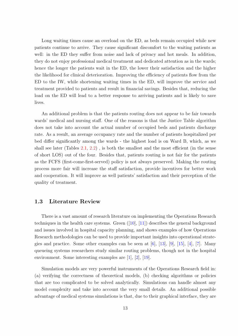
Long waiting times cause an overload on the ED, as beds remain occupied while new
patients continue to arrive. They cause significant discomfort to the waiting patients as
well: in the ED they suffer from noise and lack of privacy and hot meals. In addition,
they do not enjoy professional medical treatment and dedicated attention as in the wards;
hence the longer the patients wait in the ED, the lower their satisfaction and the higher
the likelihood for clinical deterioration. Improving the efficiency of patients flow from the
ED to the IW, while shortening waiting times in the ED, will improve the service and
treatment provided to patients and result in financial savings. Besides that, reducing the
load on the ED will lead to a better response to arriving patients and is likely to save
lives.
An additional problem is that the patients routing does not appear to be fair towards
wards’ medical and nursing staff. One of the reasons is that the Justice Table algorithm
does not take into account the actual number of occupied beds and patients discharge
rate. As a result, an average occupancy rate and the number of patients hospitalized per
bed differ significantly among the wards - the highest load is on Ward B, which, as we
shall see later (Tables 2.1, 2.2) , is both the smallest and the most efficient (in the sense
of short LOS) out of the four. Besides that, patients routing is not fair for the patients
as the FCFS (first-come-first-served) policy is not always preserved. Making the routing
process more fair will increase the staff satisfaction, provide incentives for better work
and cooperation. It will improve as well patients’ satisfaction and their perception of the
quality of treatment.
1.3 Literature Review
There is a vast amount of research literature on implementing the Operations Research
techniques in the health care systems. Green ([10], [11]) describes the general background
and issues involved in hospital capacity planning, and shows examples of how Operations
Research methodologies can be used to provide important insights into operational strate-
gies and practice. Some other examples can be seen at [6], [13], [9], [15], [4], [7]. Many
queueing systems researchers study similar routing problems, though not in the hospital
environment. Some interesting examples are [1], [2], [19].
Simulation models are very powerful instruments of the Operations Research field in:
(a) verifying the correctness of theoretical models, (b) checking algorithms or policies
that are too complicated to be solved analytically. Simulations can handle almost any
model complexity and take into account the very small details. An additional possible
advantage of medical systems simulations is that, due to their graphical interface, they are
13

understandable and useful to medical staff and not only to OR researchers. An interesting
example of simulations in health care can be viewed in Sinreich and Marmor [15], who
created a generic simulation model of an ED.
In order to discuss the various criteria for fairness we had first to obtain some insight
on the notion of fairness (justice and equity are alternative terms) in service systems in
general, and in our process in particular. We have surveyed some of the existing literature
on measuring fairness in queues ([3], [14], [17] are a few examples), which addresses fairness
from the customers point of view (for example, single queue versus multi-queues, or FCFS
versus other queueing disciplines). Different aspects are investigated, but all agree that
FCFS policy is essential for justice perception.
The literature on justice from the servers point of view is concerned with Equity
Theory, according to which the workers perceive the level of justice they are treated with
by comparing their and others ratios of the outcomes from the job and the inputs to the
job. If the outcome/income ratio of the individual is perceived to be unequal to others,
then inequity exists. The larger the inequity the individual perceives (either underreward
or overreward), the more uncomfortable he or she feels and the harder he or she works
to restore equity [12]. In [5] it is shown that in customer service centers, servers’ equity
perception has a positive influence on their performance and job satisfaction.
14

2 Model Description
In order to simulate patients flow from the ED to the four IW’s, we model the process as
a queueing system with four heterogeneous pools of servers, where pools are wards, servers
are beds, and service rates are the reciprocals of average lengths of stay (ALOS). Upon an
arrival to the system, a patient is assigned to one of the four queues (corresponding to the
four wards A-D) according to some routing algorithm, where he or she waits for admission
to the ward. In the ward the patient stays till being discharged - leaving the system.
According to this model (see Figure 2.1), we need to estimate the following parameters
for our simulation: average rate and distribution of arrivals, capacity and LOS distribution
of each ward, and waiting time for admission to the wards. The detailed description of
the chosen model and its parameters follows below; we return to it in Section 3.2 as well.
Figure 2.1: Simulation Model
15

2.1 Data Collection and Analysis
For estimating the model parameters we use empirical data collected by [8] in 2006-
2007 and, mainly, data from the Rambam information system on the years 2004-2007.
Below we describe the data used to estimate the simulation parameters: arrivals to the
system; the IW operational measures: number of beds, LOS; waiting times at the ED for
transfer to the IW.
Arrivals: Due to the extreme complexity of modeling the ED explicitly, we exclude it,
and analyze the system from the point where the decision of hospitalization is made. Thus,
arrivals to the system are patients, whom the ED decides to hospitalize in one of the four
IW (as mentioned earlier, Ward E is currently excluded from the simulation). We do not
model different patient categories in the simulation, hence the arrivals are homogeneous.
Patients arrive according to a time-dependent Poisson process with rate λt. The average
arrival rate varies across the hours of the day, days in a week and months in the year;
we model though only the weekly variation for simplicity (see Figure 2.2). On average 20
patients are hospitalized in wards A-D per day, which is around 15 percent of all patients
arrived to the internal ED. The assumption of Poisson distribution of arrivals to the ED
is commonly used in the literature (see [15], [4]), as these arrivals are unscheduled. We
confirm the compatibility of Poisson distribution with the help of JUMP software (see
example of analysis for Sunday in Figure B.1 in Appendix B).
Figure 2.2: Arrivals to Wards
13
16
19
22
25
Sun Mon Tue Wed Thu Fri Sat
Day of Week
No'
of p
atie
nts
16

Internal Wards: Usually the capacity of each medical unit is measured by its number
of beds (static capacity) and number of service providers - doctors, nurses, administrative
staff and general workers (dynamic capacity). It is common practice to assume that
the latter is proportional to the former; hence usually a unit operational capacity is
characterized by the number of its beds only (see, however, [13]). The overall capacity of
the IW’s (omitting Ward E) is 166 beds, but in overloaded periods wards occupancies can
go beyond this number, due to extra beds that can be placed in corridors. The standard
and maximal static capacity (number of beds) of the wards can be viewed in Table 2.1
below:
Table 2.1: Standard and Maximal Capacity (# beds) of the Internal Wards
Ward A Ward B Ward C Ward D Ward E
Standard capacity 45 30 44 47 24
Maximal capacity 52 35 44 48 27
Maximal to standard ratio 115% 116% 100% 102% 113%
The four wards differ not only in their capacities, but in their service times - Lengths
of Stay - as well. In Table 2.2 we see that Ward B, that is the smallest ward out of the four
(its size is just about 2/3 of the others), has Average Length of Stay (ALOS) significantly
shorter than in the other wards. Distribution of LOS is log-normal - see analysis for one
of the wards in Figure B.2 in Appendix B.
Table 2.2: LOS (days) in the Internal Wards
Ward A Ward B Ward C Ward D
Average 6.845 4.99 6.473 6.472
Standard deviation 7.621 6.398 8.252 7.864
Waiting times As we mentioned earlier, we do not have updated empirical data on
waiting times. Hence we need to estimate them based on qualitative data available to us
and common sense. In classic queueing systems waiting times are caused by unavailability
of servers - a customer in queue waits till some customer in service will leave. As servers
in our process are beds (and not medical or nursing staff), this is not the case here: even
when there are available servers (beds), a customer (a patient) usually is not admitted
to the ward immediately, but waits some time determined by the ward to which he or
17

she is allocated. Thus we divide waiting times into two phases: waiting when there is an
available bed (the so-called “boarding time” that ward staff requires for preparation, as
explained in Section 1.2); and waiting when all the beds are occupied (which is not very
common).
For the first phase, building a reliable model that will account for all the parameters
is not an easy task, particularly, when lacking empirical data. One needs to take into
account various parameters mentioned earlier (nurses and doctors availability, equipment
availability, etc.) which are hard to estimate. From the nurses in the IW we learn
that, generally, waiting time depends on the load the ward staff is subjected to at the
point of allocation time (it makes perfect sense that the higher the load, the smaller
the staff and equipment availability). The ward load can be partially described by its
occupancy rate: the more patients hospitalized in the ward, the busier its staff. Hence we
decide to model the waiting time of patient, who is allocated to Ward i (i ∈ {1, 2, 3, 4}corresponding to A-D) at time t, as an exponentially distributed random variable with
mean θi(t) = 0.5+3.5 ·ρi(t) (in hours), where ρi(t) is occupancy rate (number of occupied
beds divided by the total number of beds) of Ward i at time t.
The idea behind such modeling is as follows: it is reasonable to assume that waiting
times are exponentially distributed (see [8]). It remains to estimate the mean: if the
occupancy of the ward is close to maximal, in our model, patients will wait on average
almost four hours - and this is a maximal time within which a ward is obliged to admit
a patient. We estimate that basic preparations take around half an hour, and then the
higher the occupancy is, the longer the patient will wait. Again we should emphasize
that such modeling is not accurate, but, in our opinion, presents a simple and intuitive
attempt to simulate waiting times while accounting for load on the wards’ staff. The
assumption of dependance of waiting times on occupancy rate, as well as minimal and
maximal times, are derived from conversations with hospital factors; the assumption of
linear dependance is taken for simplicity.
18

3 Simulation Description
One can see that the proposed model is too complex to be analyzed analytically,
especially when using complicated policies for patients routing. In these cases stochastic
simulations can be a very powerful instrument for system performance analysis. With the
help of simulations one calculates various system measures sample paths throughout a long
period of operation and, by analyzing these sample paths, estimates system performance
for different scenarios and policies. We implement the simulation in the Matlab software.
3.1 Modules and Design
The objective of the simulation design is to implement a generic flexible infrastructure
for the simulation, which can be used for a wide variety of system models. This objective
can be divided into the following demands:
• The simulation structure and time advancement mechanism should be insensitive
to the implemented network structure and parameters.
• The simulation should support any network structure imposed by the system’s
model.
• The simulation should support a wide variety of routing and scheduling mechanisms.
• The simulation should support a wide variety of sample mechanisms (distributions).
• The simulation should allow long periods of operation for complex models and still
provide full system and patients histories throughout the operation period.
Another important aspect in simulation design is automation. In order to calculate and
compare system performance for a wide variety of routing policies in finite time, we ought
to implement an automated ability to run, collect data and analyze several policies in one
simulation batch.
The proposed simulation design is composed of three layers, as can be seen in Figure
3.1. We shall describe them from top (Automation and management layer) to bottom
(Network simulation layer).
19

Figure 3.1: Simulation Infrastructure
Automation and management layer: This is the external green layer in Figure
3.1. The purpose of this layer is to automatize the process of building different scenar-
ios, running them through the network simulator (see below), collecting the appropriate
information and analyzing it. A typical management layer operation includes reading
the user scenario requirements from the Main Run process. Scenario parameters include:
system definition (in M. (Matlab) file format, see Scenario simulation layer below), re-
quested priority discipline and routing algorithm. The Main Run feeds each scenario to
the Sym Main process in the Scenario simulation layer which runs the simulation. After
all the scenarios are processed, Main Run activates the Analyze Main process which an-
alyzes the simulation data. Due to the computer memory constraints all of the system’s
and customers’ information during network simulation is saved in excel format files (csv
format), which can then be filtered and analyzed by Analyze Main. The Analyze Main
process produces and saves all the system’s requested statistical data and charts for each
scenario. In this research the scenario data were collected during a system’s operational
time of 10,000 days, and was analyzed after reduction of the first 1,000 days as a warm-up
period (in order to reach steady state). The main processes (each one corresponds to the
Matlab file with the same name) in this layer are:
Main Run - This is the main M. file from which the simulation is executed. A user
inputs the requested batch of runs including systems, routing and priority methods for
each run. This batch of runs then passes on to be processed by the network simulator
sequently. There is no feedback information since the simulator information is saved in
the csv files in the computer Hard-Drive. The information for a typical batch of runs may
20

exceed 1-2 Gbyt.
Analyze Main - From this M. file the simulation analysis is executed. The user inputs
the batch of information to be analyzed, including systems, routing and priority methods.
This batch passes on to be processed by the Analyze Results sequently. The analyzed
information is then gathered and compared.
Analyze Results - This M. file reads all the csv files of each scenario from the spec-
ified location, filters and analyzes the information. The relevant information includes
customers’ entrance time to each object (server/buffer) in the network, and the system
occupancy rate at each time point. From this we can calculate and compare means and
variances of LOS, waiting times for the transfer to the wards, wards occupancy rate, and
so on.
Scenario simulation layer: This is the blue layer in Figure 3.1. The purpose
of this layer is to prepare the requested scenario for the network simulator. The main
process in this layer is the Sym Main. This M. file gets the requested system, routing and
priority from the Main Run, loads the appropriate system data which is saved in Matlab
workspace file format (.mat), sets up the arrival rate vector (which can vary with time),
and the simulation run time and warm-up time.
System definition (.mat file) includes:
• Defining the number of objects or nodes in the system network.
• Defining the role of each node - service station, buffer, entrance node, departure
node.
• Defining connections between the nodes with the help of two matrices. The first
matrix contains precedence constraints, and is denoted as “Fork-Join connections”.
The second matrix contains probabilities according to which routing is done, and is
denoted as “Jackson connections”.
• Defining for each service station the requested amount of servers, service time dis-
tribution, mean and variance.
Network simulation layer: This is the purple layer in Figure 3.1. This layer is the
stochastic network simulation for a specific scenario and system. It receives the requested
scenario and system, simulates system operations throughout long periods of time and
saves system information in the csv format on the computer HD.
21

The simulation operates according to the event-driven methodology. We define event
as the departure time of a customer from one of the system service stations or from
the entrance node (which means entrance to the system). The simulation layer receives
system parameters, including the number of nodes in the system network (node may be
a service station or a buffer) and the connection between the nodes by routing matrices
(Fork-Join and/or Jackson). At each time step of the simulation there occurs a transition
of customers between nodes. There may be two kinds of transitions - customer leaves
service station (after service completion) and enters the following buffer (or buffers for
fork nodes), or customer enters service in some station and leaves the preceding buffer.
After finishing all the current customer transitions, the event vector is updated and the
next time step is set to be the minimum time event (a more detailed definition can be
found below).
Let us define e = [e1, . . . , eN+1] as the event vector, where N is the number of service
stations in the system. ei ∀i ∈ {1, . . . , N} denotes the next customer departure time
from station i, and eN+1 denotes the next departure time from the entrance node - which
means the next customer entrance time to the system. Now let us describe the simulation
operation’s algorithm at each time step:
• Step 1 - Find the customer whose departure1 time is the current step time. There will
be only one departure - the probability of two simultaneous departures is negligible.
Send the departing customer to Routing Manager in order to route him to the
appropriate buffer or buffers2.
• Step 2 - Check all service stations for idle servers - if there is at least one idle server,
try to get another customer to be served. The non-idle condition and priority
disciplines are carried out by the Get Client From Buffer module. Every customer
accepted for a service in one of the service stations, is assigned to the Server module
for calculation of his service duration.
• Step 3 - Update the system and customer’s data and save it to the HD when needed
(if the data exceed certain size on disc). Calculate the new event vector3 e and
define next step time as min(e).
The advantage of this methodology is that the time steps are set adaptively to the
system, in contrast to a fixed-step time, which may miss some of the system events if they
1Remember that customer’s arrival to the system is defined as a departure from the entrance node.2A customer may be routed to more than one buffer at once in the case of fork nodes.3Collect from all of the service stations the next customer departure time - ei ∀i ∈ {1, . . . , N}, and
from the entrance node the next customer arrival - eN+1.
22

are too dense in time. In addition, it can be seen that this simulation implementation is
insensitive to the requested network structure and parameters. Let us describe the main
processes in this layer:
Net Analyze - This is the main simulation engine. Its operation is described above (by
the above three steps). This module’s input is the scenario and system received from Sym
Main, and its output is the csv files which are created throughout the entire simulation’s
operation (this way clearing computer memory during the run) and contain system and
customer information.
Routing Manager - This module is in charge of the routing discipline. The input to this
module is the departure client and the station from which he departs. Then the routing
is performed according to Fork-Join discipline and/or Jackson discipline or by some hard-
coded algorithm. By this variety of options we can perform any routing discipline needed
including Feedback and close-loop algorithms. The change in a customer’s location in the
network is then updated in the network data structure.
Get Client From Buffer - This module is in charge of the non-idle condition and the
priority discipline; its job is to move customers from the preceding buffers to the service
stations, whenever possible. As in the Routing Manager, the priority discipline can be
any given algorithm, including close-loop and time-varying algorithms. In addition every
given station in the system can have its own different priority discipline.
Server - This module generates an appropriate distribution sample for customers’
service duration. The input to this module is the server’s properties, including distribution
type, mean and variance parameters. In our implementation the module can generate
samples for exponential, deterministic and log-normal distributions.
3.2 Model Implementation
First we intended to model the system from customers’ arrival to the ED till their
departure from the wards. However, we soon realized that, in order to have a good
approximation of the customers’ departure process, we need to have a precise model of
the ED, which is extremely complex. Consequently we decided to focus on the transition
process from the decision on hospitalization in the ED till the departure from the wards.
As can be seen in Figure 3.2 the customers’ flow has three main stages:
23

Figure 3.2: System
ED Departure and Routing: The entrance process interarrival distribution is im-
plemented according to empirical data from the ED (see Section 2.1). The entrance
to the simulation is taken to be the ED departure process for hospitalized patients,
meaning patients which were admitted to the wards. Empirical distribution presents a
time-dependent Poisson process, and is implemented according to exp(λ(t)) = 1λ(t)
exp(1).
Therefore x(t) = 1λ(t)
y = − 1λ(t)
log(u), where x is a sample of the non-homogeneous Pois-
son process with rate λ(t), y is a sample of the homogeneous Poisson process with rate 1
and u is a sample of the standard uniform distribution. As can be seen, the sample x(t) is
a function of the current time t according to λ(t), and therefore is updated at each time
step to the appropriate value.
The arriving customers are sent immediately to the Routing Manager module in order
to be routed according to some algorithm as we shall describe in Section 4. The routed
patients then enter the transition stage.
Transition Stage: In this stage all the patients are assigned to a certain ward (cur-
rently patients cannot change wards after the first decision was made). As discussed in
Section 2.1, in order to be admitted to a ward, the patients need to wait in the ED for two
conditions to be fulfilled: first, there should be an available bed for the arriving patient;
24

second, there exists an additional delay caused by nurses’ and doctors’ unavailability. We
learn that the second delay is commonly influenced by the ward’s occupancy, and the
mean wait duration is between one-half hour to four hours. Consequently, this stage is
implemented by two levels of delay - first, after being assigned to ward i (i ∈ {1, . . . , 4})the patient enters a transition “service station” with an infinite number of servers with
exponentially distributed service times with mean θi(t) = 0.5 + 3.5 · ρi(t), where ρi(t) is
the occupancy rate of Ward i at time t. Then the patient enters the ward resource buffer
which enforces the condition of available beds (we consider beds as servers).
Hospitalization in the Wards: After the transition stage the patient is hospitalized
in a ward. As was discussed in Section 2.1, the wards are service stations with a spec-
ified number of servers (beds) whose service time distribution is log-normal with mean
and variance found empirically. We implement the log-normal distribution by using the
relation y = eµ+σ·x, where y is distributed log-normal and x is a sample from standard
normal distribution. For given log-normal parameters {E(y), V ar(y)} - which are given
by the empirical data in Section 2.1 - we can calculate the required normal distribution
parameters µ = eE(y)+V ar(y)/2 and σ =√
eV ar(y) − 1 · eE(y)+V ar(y)/2.
3.3 Validation Versus Empirical Data
After the process of writing and debugging the code is successfully finished, the next
thing to do is to verify that the implementation indeed follows our intentions. Namely,
we should validate the simulation results versus the empirical data - and that is what this
subsection is about.
Arrivals and Departures: The customer arrival is a stochastic process which is im-
plemented in the simulation. Additionally this process is time-dependent, which increases
the implementation complexity4. The customer departure is a stochastic process which is
produced from the arrival process and from the customer flow through the system. The
following tests are statistical tests on the simulation output data whose purpose is to check
the implementation of these processes. First of all we verify that the average number of
arrivals on each day of the week in the simulation equals the empirical average number
of admissions to wards A-D (see Figure 3.3). Second, we wish to verify that the arrivals
distribution is Poisson, or that inter-arrival times distribution is exponential. For that
purpose we examine histograms of inter-arrival times between the sequential entrances
4The problem with time-dependent processes is inaccurate results due to the simulation time-steps;our implementation is designed to overcome this problem.
25
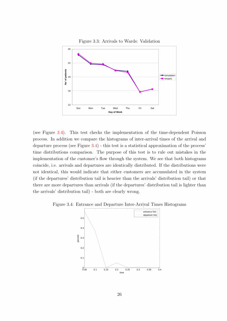
Figure 3.3: Arrivals to Wards: Validation
13
16
19
22
25
Sun Mon Tue Wed Thu Fri Sat
Day of Week
No'
of p
atie
nts
simulationempiric
(see Figure 3.4). This test checks the implementation of the time-dependent Poisson
process. In addition we compare the histograms of inter-arrival times of the arrival and
departure process (see Figure 3.4) - this test is a statistical approximation of the process’
time distributions comparison. The purpose of this test is to rule out mistakes in the
implementation of the customer’s flow through the system. We see that both histograms
coincide, i.e. arrivals and departures are identically distributed. If the distributions were
not identical, this would indicate that either customers are accumulated in the system
(if the departures’ distribution tail is heavier than the arrivals’ distribution tail) or that
there are more departures than arrivals (if the departures’ distribution tail is lighter than
the arrivals’ distribution tail) - both are clearly wrong.
Figure 3.4: Entrance and Departure Inter-Arrival Times Histograms
0.05 0.1 0.15 0.2 0.25 0.3 0.35 0.40
0.1
0.2
0.3
0.4
0.5
time
perc
ent
Entrance and Departure Inter-Arrival Times Histograms
entrance histdeparture hist
26

LOS: Next we check that the time spent in the wards in the simulation equals empiric
LOS. We compare means and standard deviations of LOS, obtained from simulation versus
empirical. We see that the means are very accurate, and standard deviations are accurate
for wards A and D, and slightly less accurate for wards B and C. In addition we test
whether the LOS distribution in the simulation is indeed log-normal. In Figure 3.5 we
compare empiric and simulation LOS histograms for Ward A (for other wards we obtain
similar results).
Figure 3.5: LOS Distribution Validation (LOS in days)\\
0 10 20 30 40 50 600
0.02
0.04
0.06
0.08
0.1
0.12
0.14Ward A LOS Histogram - Simulation Ward A LOS Histogram - Empiric
0
0.02
0.04
0.06
0.08
0.1
0.12
0.14
0 4 8 12 16 20 24 28 32 36 40 44 48 52 56 60
simulation empiric
Ward A Ward B Ward C Ward D
Empiric 6.845 4.990 6.472 6.472 Simulation 6.890 4.966 6.437 6.481
Empiric 7.621 6.398 8.252 7.864 Simulation 7.603 5.618 7.038 7.369
Mean
St.Dev.
Occupancy Rate: This test is more significant than the previous ones: there, as
arrivals and LOS were generated initially with the empirical data, we test mainly that
the implementation of the distribution is correct. Here we check that the logic behind the
simulation works correctly. For testing, we take the routing policy which, as far as we are
concerned, reflects the actual situation in the hospital. As we described in Section 1.2,
the Justice Table algorithm routes according to “fixed turns” among the wards, namely
each ward receives one patient in its turn, while accounting for ward capacities (we denote
such routing RR 3233 and return to it for a detailed explanation in Section 4).
In Figure 3.6 we see that the simulation provides accurate results for wards A and D,
but less accurate results for the other two wards. The explanation for this inaccuracy is
that, first of all, we do not account for different patients categories, while routing in the
Justice Table is done independently for each category. In addition the actual routing is not
27
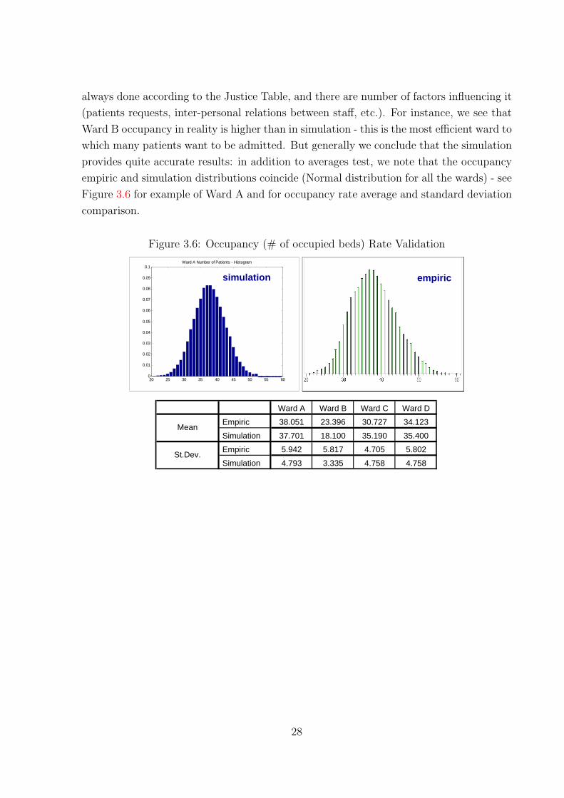
always done according to the Justice Table, and there are number of factors influencing it
(patients requests, inter-personal relations between staff, etc.). For instance, we see that
Ward B occupancy in reality is higher than in simulation - this is the most efficient ward to
which many patients want to be admitted. But generally we conclude that the simulation
provides quite accurate results: in addition to averages test, we note that the occupancy
empiric and simulation distributions coincide (Normal distribution for all the wards) - see
Figure 3.6 for example of Ward A and for occupancy rate average and standard deviation
comparison.
Figure 3.6: Occupancy (# of occupied beds) Rate Validation
20 25 30 35 40 45 50 55 600
0.01
0.02
0.03
0.04
0.05
0.06
0.07
0.08
0.09
0.1Ward A Number of Patients - Histogram
simulation empiric
Ward A Ward B Ward C Ward D
Empiric 38.051 23.396 30.727 34.123
Simulation 37.701 18.100 35.190 35.400
Empiric 5.942 5.817 4.705 5.802
Simulation 4.793 3.335 4.758 4.758
Mean
St.Dev.
28
4 Algorithms
In this section we shall define, implement and compare various algorithms for the
patients routing. We take into account three main concerns when implementing and
testing algorithm performances:
• System performance - Achieving good system performance (minimal waiting and
sojourn time);
• Sociological aspects - Inducing fairness from staff and patients’ points of view on
the system’s operation;
• Control system design - System design should be appropriate to the ability to
access system’s operational information (full continuous access, partial access, no
information).
In Section 4.1 we shall define various performance criteria and in Section 4.2 “trans-
late” them into quantitative measures and deduce a single integrated criterion of quality,
which will be used to estimate and compare algorithm performance. In Sections 4.3 and
4.4 we shall discuss the proposed algorithms and the results they achieved.
4.1 Performance Criteria (qualitative)
In order to evaluate different routing policies and compare them we should define an
optimality criterion. This criterion includes various measures that are mainly divided into
fairness measures and performance measures. We strive to obtain a single quantitative
measure that will aggregate those measures with appropriate weights - we denote it as
the “integrated criterion of quality”.
Possible criteria for fair patient allocation, from alternative points of view, are abun-
dant. We look at various criteria from three main points of view: wards - meaning medical
and nursing staff, patients, and administration or management. Using results of a survey
conducted by [8], in which the staff (nurses, doctors and administration) were asked to
grade the extent of fairness in different routing policies, and common sense, we choose to
focus on the following criteria:
It is obvious that, talking of fairness to nursing staff, one should ensure that each
nurse has the same workload. Seemingly it is the same as to say that each nurse takes
29

care of an equal number of patients. Under the assumption that the number of nurses
is proportional to the standard capacity, this criterion is the same as keeping occupancy
rates equal among the wards. Thus the “wards equal occupancy” is treated as the main
criterion for fair allocation, but is it the only right criterion?
As we saw earlier, ALOS differs significantly across the wards. If we keep the occu-
pancy levels equal, wards with shorter ALOS will have a higher turnover rate - admit
more patients per bed. But the load on the wards staff is not uniform during a patient’s
stay - treatment during the first days of hospitalization requires much more time and
effort from the staff than in following days [8]. Thus, even if the occupancy of the wards
is kept equal, the ward receiving more patients per bed has a larger load on its staff.
Consequently, a ward might develop an interest in prolonging its existing patients’ stay
because, by keeping equal occupancies, it will have to admit less new patients, and thus
reduce its load. Not only do the wards have no incentive to make their processes more
efficient - actually, they have an incentive to become less efficient (prolong their ALOS)-
surely a result that no one wishes to see happening in health care. Then ALOS should be
accounted for in fair routing policies by compensating the faster and more efficient ward.
Hence, besides balancing the load implied by hospitalized patients, we wish to balance
the incoming load (or the flow rate): the number of patients per bed per certain time
unit (for example, per year) should be the same among the wards. This way we account
for the wards’ size and service rates. Besides that, one should take into account time
that passed since each ward received its last patient (it would not make sense to send two
patients in a row to the same ward, as the process of a patient’s admission takes time and
resources). Combining these two criteria, it makes sense to send a patient to the ward
that has not received patients for the longest time, accounting for the wards’ capacities.
Fairness criteria from the patients’ point of view is concerned mainly with waiting time
from hospitalization decision till admission to the ward: we expect it not to vary much
among the patients. Ensuring that each nurse takes care of an equal number of patients
is a criterion of interest here as well, as this way each patient should receive equal quality
of treatment. From the managerial point of view the main fairness criterion is keeping
occupancy rates equal among the wards.
In order to measure how fair each policy is according to a certain criterion, we can use
the standard deviation of the parameter that we wish to balance (see [18], who measured
the fairness of airport schedules in a similar way). For example, for the criterion of
balanced occupancy rates the quantitative measure will be the average standard deviation
of occupancy rate and for the criterion of balanced flow rates it will be the standard
30

deviation of flow rate. In order to measure the fairness for patients, we can use standard
deviation of the waiting time (similar to [3]). See Section 4.2 for quantitative definitions.
As for operational performance criteria, we take as a main measure the waiting time:
for reasons we described above (see Section 1.2) it is important to discharge patients from
the ED efficiently, thus reducing the load on the ED and improving patients’ quality of
treatment. As an alternative performance measure we shall consider the sojourn time in
the system: waiting time together with hospitalization time (LOS). This measure receives
less importance, as lengths of stay in our model are invariant to different routing policies
(while in reality they certainly might, as some policies provide incentives to the wards
to discharge patients quicker, and others on the opposite - interesting point for future
research - see Section 6). Waiting times are significantly smaller than LOS (hours versus
days) thus they do not play much difference in sojourn times.
Summarizing, below are the main criteria that form our integrated criterion of quality:
1. Minimal average standard deviation of occupancy rate of the wards;
2. Minimal standard deviation of number of patients per bed per year (flow rate) in
the wards;
3. Minimal waiting time;
4. Minimal sojourn time;
5. Minimal standard deviation of waiting time of patients;
6. Minimal standard deviation of sojourn time of patients.
In the next subsection we translate the criteria into a quantitative way, and obtain one
weighted optimality criterion.
4.2 Performance Criteria (quantitative)
It is easy to see that the criteria, qualitatively defined above, involve different measures
and contradicting demands on the system performance measures. In order to achieve an
acceptable integrated criterion of quality, we need to define the quantitative measure for
each criterion and calculate an average with adjustments for the relative importance of
each element (weights). Let us define the quantitative representation of the criteria:
31

Indices:
• Wards: i = 1, 2, 3, 4
• Patients: k = 1, 2, . . . , K
• Time: T = {t1, t2, ..., tn} is the set of all event points in the simulation
Parameters:
1. Constant
• N sti - standard capacity (number of beds) of ward i
2. Wards’ staff:
• Li(t) - number of patients admitted in ward i from time 0 till time t
• Ni(t) - number of occupied beds in ward i at time t
• ρi(t) - occupancy rate in ward i at time t: ρi(t) = Ni(t)N sti
• γi(t) - patient flow rate through ward i till time t: γi(t) = Li(t)N sti
• γi - average patient flow rate through ward i per one year: γi = γi(tn)tn/365
• Sd(ρ(t)) =√
13
∑4i=1 (ρi(t)− ρ̄(t))2 - estimated standard deviation of the oc-
cupancy rate (ρ̄(t) =P4
i=1 ρi(t)
4denotes an average occupancy)
• Meant∈T{Sd(ρ(t))} - average standard deviation of the occupancy rate
• Sd(γ) =√
13
∑4i=1 (γi − γ̄)2 - estimated standard deviation of the flow rate
(γ̄ =P4
i=1 γi
4denotes an average flow)
3. Patients:
• w1k - Waiting time of patient k since the decision of his hospitalization till
entrance time to a ward.
• w2k - Total sojourn time of patient k in the system.
• Sd(w1) =√
1K
∑Kk=1 (w1
k − w̄1)2 - estimated standard deviation of the patients’
waiting time, where w̄1 is the average waiting time of all the K patients.
• Sd(w2) =√
1K
∑Kk=1 (w2
k − w̄2)2 - estimated standard deviation of the patients’
sojourn time, where w̄2 is the average sojourn time of all the K patients.
32

Integrated criterion of quality: Next we define the quantitative integrated criterion
of quality (as presented qualitatively in Section 4.1) that we aim to minimize:
G(T ) =α1 ·Meant∈T{Sd(ρ(t))}+ α2 · Sd(γ) + α3 · w̄1+
+ α4 · w̄2 + α5 · Sd(w1) + α6 · Sd(w2),
where αi, i ∈ {1, 2, ..., 6} are relative weights of the criteria (∑6
i=1 αi = 1). The vec-
tor {αi} can have a degenerated version in which αi = 1, for some i ∈ {1, . . . , 6} and
αj = 0,∀j 6= i, meaning only a single criterion is taken into consideration. The choice of
appropriate weights is subjective and may affect the evaluation of the algorithms perfor-
mance.
4.3 Algorithms description and results
Another parameter we need to account for when choosing the routing policy, is the
availability of information in the system in the moment of the routing decision. We look
at three possibilities: no information, meaning that when taking a routing decision we
know only static parameters (standard capacity, ALOS), and the system’s actual state is
unknown to us; full information, meaning that dynamic system parameters, like wards’
occupancy rate, are available to us; and partial information, meaning that we know the
system’s state at some time points (for example, the occupancy in the morning) and we
estimate its state at the decision time based on this information.
4.3.1 No Access to System Information
Round-Robin Policies: The wards accept patients according to a predefined deter-
ministic cycle; this method is very simple to implement and intuitive to comprehend, and
it is widely used in routing policies in various hospitals.
RR 1111
Algorithm Description
According to this policy the wards admit patients in turns, when at each turn the ward
admits a single patient. This method is actually equivalent to the policy that assigns to
the ward that received its last patient the longest time ago, since at each step the ward,
that admits a patient in its turn, has received its last patient the longest time ago. It
can be seen that this policy does not consider the difference in ward capacity nor the
33

difference in ward service times. Consequently, the ward whose capacity is the lowest will
suffer the highest load, which is highly unfair. However, this policy is practiced widely in
hospitals due to its simplicity and non-requirement of computer aid.
Algorithm Results
Figure 4.1: RR 1111 Occupancy Rate
Figure 4.1 shows the occupancy distribution (ρi) of each ward over the entire operational
time (which is 10,000 days not including a 1,000 day warm-up period). It can be seen
that the occupancy distribution is non-standard Normal distribution whose upper barrier
is trimmed by the wards’ maximal capacity, which allows ρi to exceed “1” (occupancies
are calculated with respect to the wards’ standard capacity). We can see that there is a
non-negligible distribution mass5 in the area of ρ = 1 especially in Ward B distribution;
this implies that ward B is overloaded. The table above represents the occupancy mean
and variance of each ward, and the variance in the wards’ occupancy. It shows us as well
that the load on the wards is not balanced and that ward B is overloaded compared to
other wards.
Figure 4.2 represents the distribution of the standard deviation of ward occupancy
- this distribution appears to be log-normal. The smaller the deviation, the more balanced
occupancy rates are among the wards. Thus the important measure here is the mass6
around zero: the larger mass around zero reflects a better balance in the wards load.
When we compare this figure to the appropriate one in other routing algorithms it will
5Distribution mass in the area of ρ = 1 may be defined by∫∞1−ε
f(t)dt, which implies the probabilitythat the load is around or above ρ = 1.
6Distribution mass in the area of zero may be defined by∫ 0+ε
0f(t)dt, which implies the probability
that the occupancy rate standard deviation is around zero.
34

Figure 4.2: RR 1111 Occupancy Standard Deviation
be clear that this method has less mass around zero than the others, again implying
unfairness.
Figure 4.3: RR 1111 Sojourn Time
Figure 4.3 represents the sojourn time distribution of the patients from all the wards. This
measure is an important one for the management, who wishes to supervise the customers’
flow through the system and enforce short sojourn times and low queue length. The
important measure is the mass around zero as well: the more distribution mass around
zero reflects faster customers’ flow through the system. The table above represents the
waiting and sojourn times mean and variance, respectively. By comparing these values
we can measure the effect of the algorithms on the customers’ flow.
35

RR 3233
Algorithm Description
According to this policy the wards admit patients in turns, when at each turn the selected
ward admits a number of patients which is proportional to its standard capacity. Meaning
that the number of patients each ward admits at its turn is derived from the ward standard
capacity divided by the joint largest integer divider which is 15 (recall Table 2.1). This
policy does not consider the difference in wards service times, thus the ward whose service
rate is the lowest will suffer the highest load. This can give the slow wards an incentive
to work faster which is generally good, but perhaps not so appropriate to the health care
system.
Algorithm Results
Figure 4.4: RR 3233 Occupancy Rate
Figure 4.4 shows that there is a non-negligible mass in the area of ρ = 1, especially in Ward
A distribution - this implies that Ward A (which has the lowest ALOS) is overloaded.
The ward which “profits” the most from this policy is Ward B, which, due to its low
capacity and high service rate enjoys a very low load in comparison to other wards. From
the table we can also see that the load on the wards is not balanced.
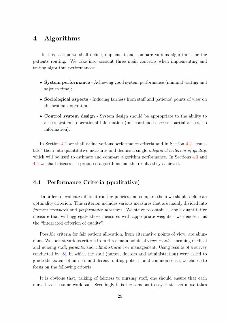
It is easy to see from Figure 4.5 that the load is unbalanced. The peak of the distribution
crossed the value of 0.1, which means that there is more distribution mass above the
Standard Deviation value of 0.1 (∫ ∞
0.1f(t)dt). This performance measure is worse than in
the previous policy.
From Figure 4.6 we can see that this policy makes the patients flow slightly slower: it
36
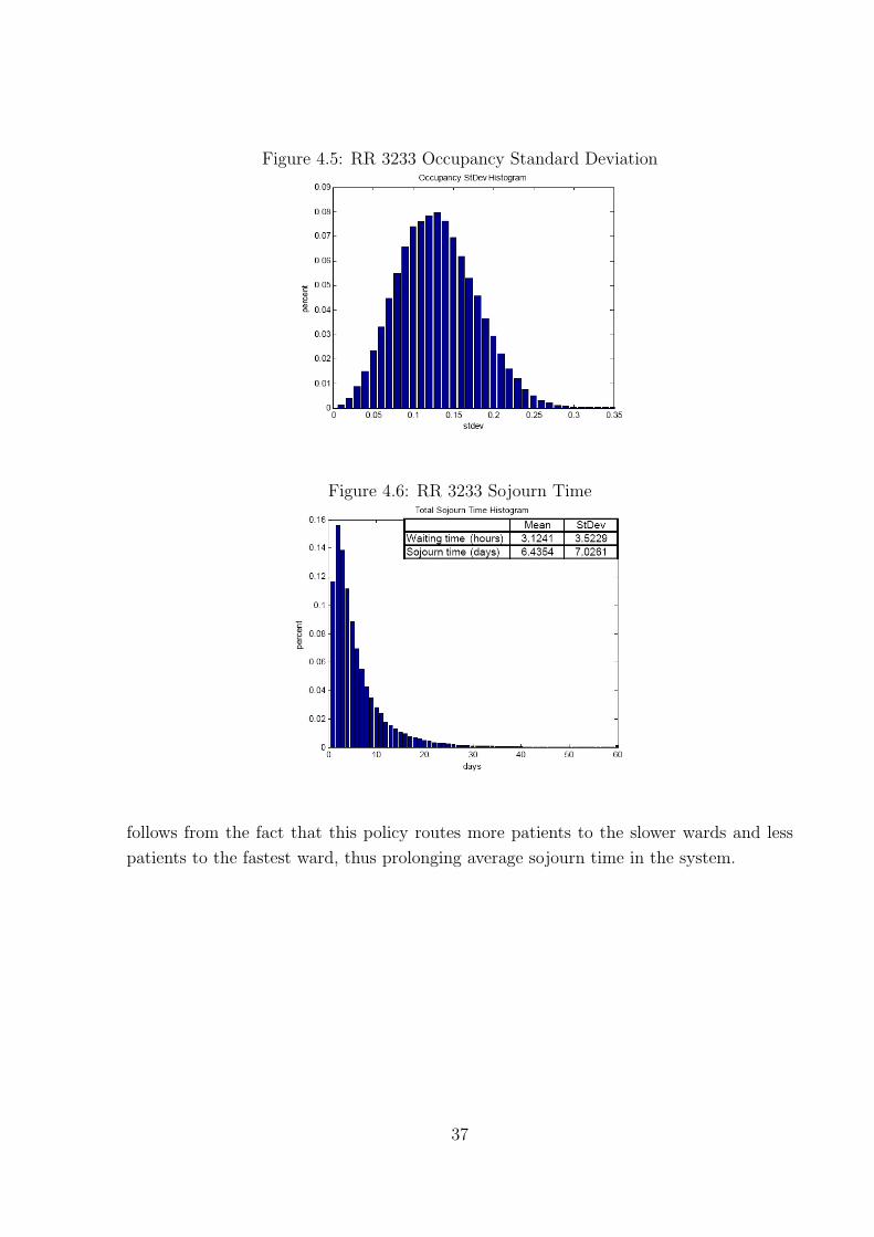
Figure 4.5: RR 3233 Occupancy Standard Deviation
Figure 4.6: RR 3233 Sojourn Time
follows from the fact that this policy routes more patients to the slower wards and less
patients to the fastest ward, thus prolonging average sojourn time in the system.
37

4.3.2 Full Information
Idleness Balancing (IB)
Algorithm Description
In this policy we route a patient to the maximal vacant ward - ward which has maximum
number of available beds. In this way the algorithm aims to keep an equal number of idle
servers in all wards. The selection of k - the ward to receive the next patient, is done
through this simple calculation:
k = argmaxi∈{1,...,4}{vacant(i) = argmaxi∈{1,...,4}{N sti −Ni}i}; (4.1)
In order to understand the expected distribution of the load between the different wards,
let us check the following scenario: The algorithm keeps an equal number of idle servers in
all stations - we denote this number by δ, then for all i ∈ {1, . . . , 4} we receive N sti−Ni =
δ. From this relation we deduce the station load ρi = Ni
N sti= N sti−δ
N sti= 1− δ
N sti. Therefore
we can conclude that the larger wards (bigger N sti) will suffer from larger loads.
Algorithm Results
Figure 4.7: IB Occupancy Rate
Figure 4.7 shows that there is a non-negligible mass in the area of ρ = 1 especially in Ward
A distribution; this implies that Ward A is overloaded. The reason can be explained due
to the ward size and the ward slow service rate in comparison to the other wards. From
the table we can also see that the maximum load is on ward A and the lowest load is on
ward C - the load on the wards is not balanced.
38
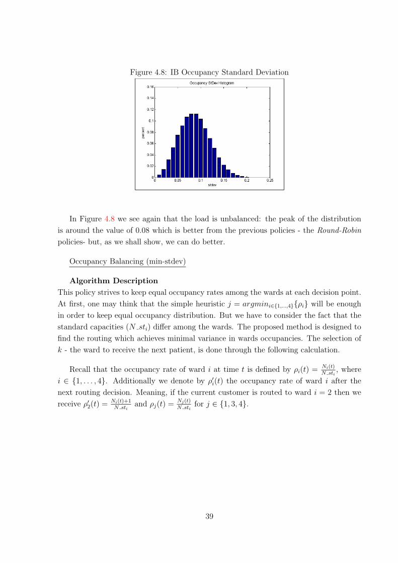
Figure 4.8: IB Occupancy Standard Deviation
In Figure 4.8 we see again that the load is unbalanced: the peak of the distribution
is around the value of 0.08 which is better from the previous policies - the Round-Robin
policies- but, as we shall show, we can do better.
Occupancy Balancing (min-stdev)
Algorithm Description
This policy strives to keep equal occupancy rates among the wards at each decision point.
At first, one may think that the simple heuristic j = argmini∈{1,...,4}{ρi} will be enough
in order to keep equal occupancy distribution. But we have to consider the fact that the
standard capacities (N sti) differ among the wards. The proposed method is designed to
find the routing which achieves minimal variance in wards occupancies. The selection of
k - the ward to receive the next patient, is done through the following calculation.
Recall that the occupancy rate of ward i at time t is defined by ρi(t) = Ni(t)N sti
, where
i ∈ {1, . . . , 4}. Additionally we denote by ρ′i(t) the occupancy rate of ward i after the
next routing decision. Meaning, if the current customer is routed to ward i = 2 then we
receive ρ′2(t) = Ni(t)+1N sti
and ρj(t) =Nj(t)
N stifor j ∈ {1, 3, 4}.
39

Then:k = argmini∈{1,...,4}Var(ρ′i)
s.t
Var(ρ′i) =√
13
∑4j=1 (ρ̄′(t)− ρ′j(t))
2.
ρ̄′(t) =P4
j=1 ρ′j
4.
ρ′i(t) = Ni(t)+1N sti
,
ρ′j(t) =Nj(t)
N st, ∀j 6= i.
(4.2)
where k denotes the ward selected to receive the next patient.
Algorithm Results
Figure 4.9: Min-stdev Occupancy Rate
It can be seen that this method effectively balances the wards’ load. Figure 4.9 shows
that the mass in the area of ρ = 1 is smaller, which means that the probability for the
wards to exceed their standard capacity is much less than in the previous policies. Also
it is clear from the figure that the different ward distributions coincide with each other.
From the table it is also clear that the wards loads under this policy become similar;
the variance between the ward occupation is 0.024 instead of 0.1 or 0.08 in the previous
policies.
It is easy to see from Figure 4.10 that the load is more balanced than before, the peak of
40
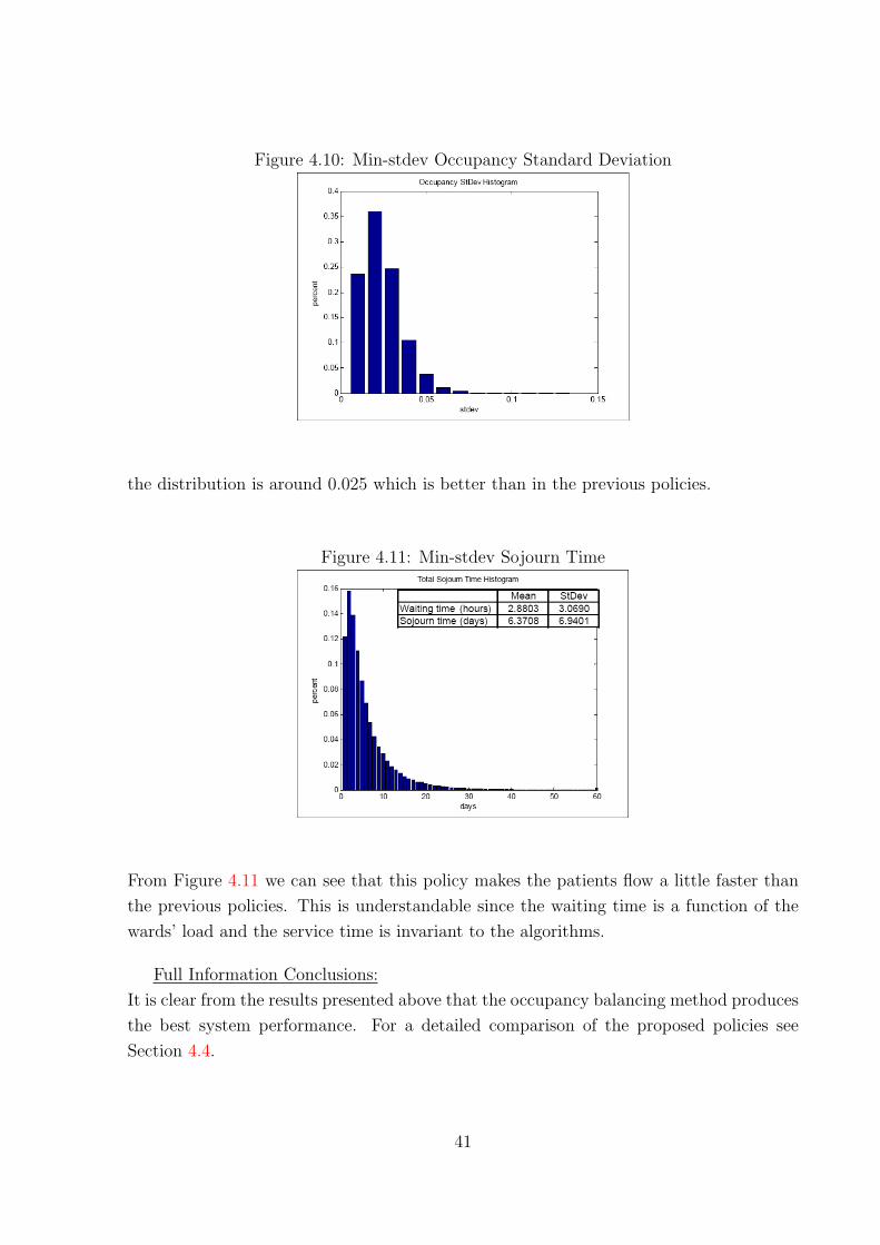
Figure 4.10: Min-stdev Occupancy Standard Deviation
the distribution is around 0.025 which is better than in the previous policies.
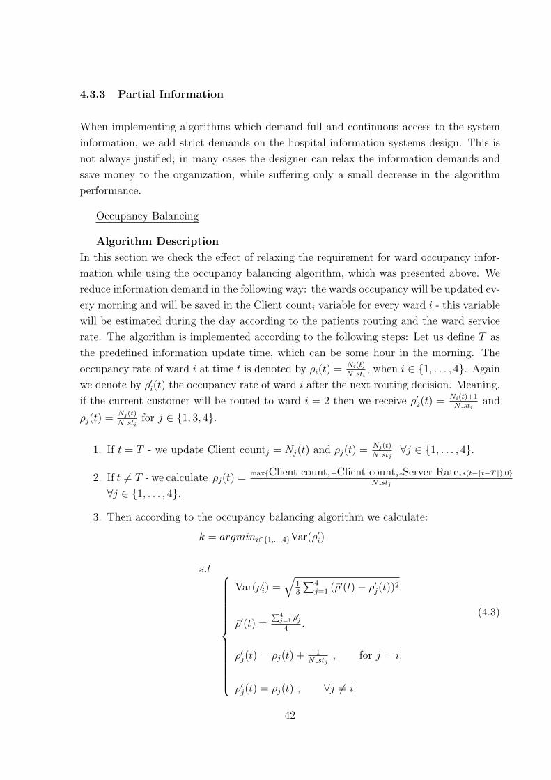
Figure 4.11: Min-stdev Sojourn Time
From Figure 4.11 we can see that this policy makes the patients flow a little faster than
the previous policies. This is understandable since the waiting time is a function of the
wards’ load and the service time is invariant to the algorithms.
Full Information Conclusions:
It is clear from the results presented above that the occupancy balancing method produces
the best system performance. For a detailed comparison of the proposed policies see
Section 4.4.
41
4.3.3 Partial Information
When implementing algorithms which demand full and continuous access to the system
information, we add strict demands on the hospital information systems design. This is
not always justified; in many cases the designer can relax the information demands and
save money to the organization, while suffering only a small decrease in the algorithm
performance.
Occupancy Balancing
Algorithm Description
In this section we check the effect of relaxing the requirement for ward occupancy infor-
mation while using the occupancy balancing algorithm, which was presented above. We
reduce information demand in the following way: the wards occupancy will be updated ev-
ery morning and will be saved in the Client counti variable for every ward i - this variable
will be estimated during the day according to the patients routing and the ward service
rate. The algorithm is implemented according to the following steps: Let us define T as
the predefined information update time, which can be some hour in the morning. The
occupancy rate of ward i at time t is denoted by ρi(t) = Ni(t)N sti
, when i ∈ {1, . . . , 4}. Again
we denote by ρ′i(t) the occupancy rate of ward i after the next routing decision. Meaning,
if the current customer will be routed to ward i = 2 then we receive ρ′2(t) = Ni(t)+1N sti
and
ρj(t) =Nj(t)
N stifor j ∈ {1, 3, 4}.
1. If t = T - we update Client countj = Nj(t) and ρj(t) =Nj(t)
N stj∀j ∈ {1, . . . , 4}.
2. If t 6= T - we calculate ρj(t) =max{Client countj−Client countj∗Server Ratej∗(t−bt−T c),0}
N stj
∀j ∈ {1, . . . , 4}.
3. Then according to the occupancy balancing algorithm we calculate:
k = argmini∈{1,...,4}Var(ρ′i)
s.t
Var(ρ′i) =√
13
∑4j=1 (ρ̄′(t)− ρ′j(t))
2.
ρ̄′(t) =P4
j=1 ρ′j
4.
ρ′j(t) = ρj(t) + 1N stj
, for j = i.
ρ′j(t) = ρj(t) , ∀j 6= i.
(4.3)
42

where k denotes the ward selected to receive the next patient.
4. Finally according to the chosen routing we update:
Client countk = Client countk + 1.
Algorithm Results
It is clear from the following graphs (Figures 4.12, 4.13, 4.14) that the results are similar
to those seen in the full information section. We can see that the partial information
is slightly inferior in the aspects of load balancing and customer flow. These differences
are clear since it is the same method as in the full information case but in that case the
routing decision relies on accurate and updated system information. However the partial
information results are very good in comparison to the full information when considering
the reduction in system complexity and design demands.
Figure 4.12: Partial-Information Occupancy Rate
43

Figure 4.13: Partial-Information Occupancy Standard Deviation
Figure 4.14: Partial-Information Sojourn Time
4.3.4 Weighted Algorithm
From the previous sections it is clear that the occupancy balancing method produces the
best results for partial and full information options. However, as discussed in Section 4.1
and as can be seen (see Section 4.4), this method has a disadvantage manifested in an
uneven number of patients per bed per year among the wards. This problem arises since
the fastest ward receives more patients according to the routing scheme in order to keep
its occupancy similar to the other wards. This effect is unfair and undesired since it will
give the fastest wards an interest in postponing patients’ discharge and prolong ALOS.
Therefore, in order to keep the wards load balanced and simultaneously to be fair to the
fastest ward we need to formulate a weighted algorithm which adjusts by weights the two
conflicting demands.
44

Algorithm Description
First we need to collect information about the patient flow in the wards. In order to do
that we require a vector of counters, which count the number of patients received in ward
i till time t; we shall denote these counters by Li(t). The period of time to accumulate
patient flow can be any long period of time, such as a year or half a year (at the beginning
of the period we set the counters to zero). In order to calculate and compare the patient
flow we shall use the definitions from Section 4.2 - customer flow rate through ward i till
time t is defined by γi(t) = Li(t)N sti
and Sd(γ(t)) denotes the estimated standard deviation
of the flow rate till time t. The method which minimizes Sd(γ(t)) will be referred as
the flow balancing method in the rest of the report. The weighted algorithm is a convex
combination of the two proposed methods: the flow balancing method and the occupancy
balancing method. The combination of the two methods is adjusted by a pair of weights
{α1, α2} which satisfies αi ∈ [0, 1] ∀i ∈ {1, 2}, α1 + α2 = 1.
The complete algorithm formulation is as follows:
Again we denote by ρ′i(t) the occupancy rate of ward i after the next routing decision. In
addition we denote by γ′i(t) the flow to ward i after the next routing decision.
k = argmini∈{1,...,4}(α1 ·√
13
∑4j=1 (ρ̄′(t)− ρ′j(t))
2 + α2 ·√
13
∑4j=1 (γ̄′(t)− γ′
j(t))2)
s.t
ρ̄′(t) =P4
j=1 ρ′j
4.
γ̄′(t) =P4
j=1 γ′j
4.
ρ′j(t) =Nj(t)+1
N stj, for j = i.
ρ′j(t) =Nj(t)
N st, ∀j 6= i.
γ′j(t) =
Lj(t)+1
N stj, for j = i.
γ′j(t) =
Lj(t)
N stj, ∀j 6= i,
(4.4)
where k denotes the ward selected to receive the next patient.
In our work we chose to use {α1, α2} = {0.5, 0.5}; any choice of weights will give differ-
ent importance to each of the criteria, and may change the resulted system performance.
One can expand our work by using gradient descent or Newton’s method algorithms in
45

order to find the weight proportions which assign maximum value to some grade function
that represents system performance. These local optimization search methods can be
applied on the continuous space defined by αi ∈ R[0,1] ∀i ∈ {1, 2}, α1 + α2 = 1, in order
to find the pair of weights which give optimal system performance measures.
Algorithm Results
As can be seen in the graphs (Figures 4.15, 4.16) below, the weighted algorithm keeps the
occupancy rates balanced and also rewards the fastest Ward B, which receives a slightly
less load. This effect compensates the occupancy balancing method’s natural tendency
to send more patients to the fastest ward - on opposite, the slowest ward (Ward A)
receives the highest load which might motivate it to improve its service rate. In addition
the positive effects of the occupancy balancing method are preserved: the occupancy
distribution figure (Figure 4.15) shows that there is little mass in the area of ρ = 1,
which means that the probability for the wards to exceed their standard capacity is low.
From the table we see that the standard deviation of the occupancy rates is 0.056 instead
of 0.024 in the pure occupancy balancing algorithm, which is slightly higher but still
much better than in the other algorithms. From Figure 4.16 we see that the peak of the
distribution is around the value of 0.05 which is still good in comparison to the other
algorithms.
Figure 4.15: Weighted Occupancy Rate
46
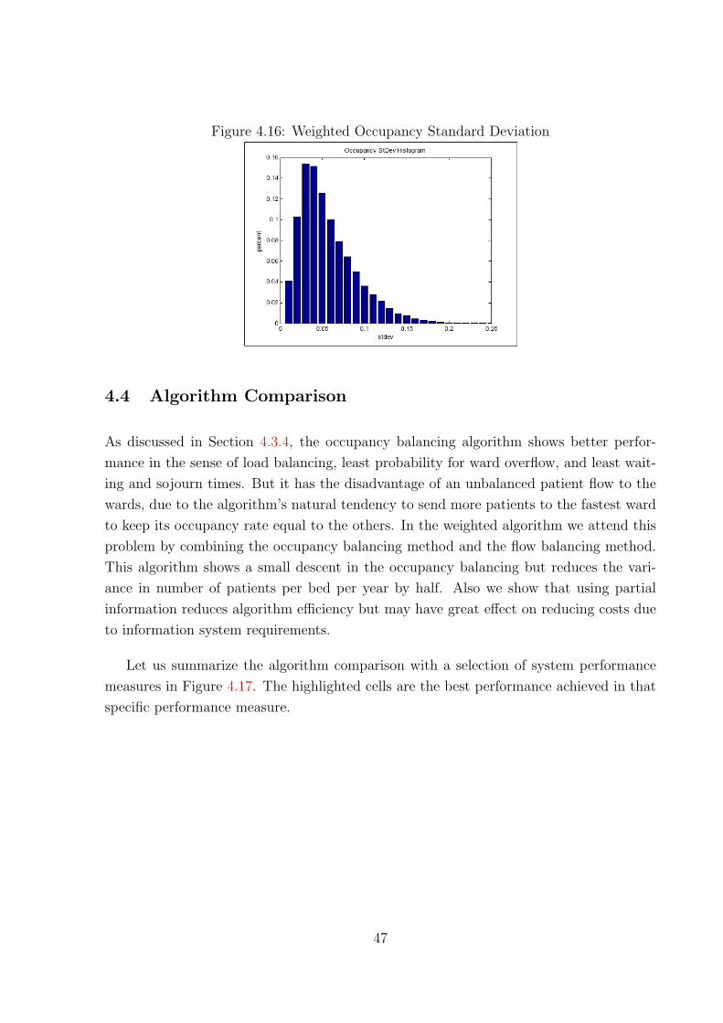
Figure 4.16: Weighted Occupancy Standard Deviation
4.4 Algorithm Comparison
As discussed in Section 4.3.4, the occupancy balancing algorithm shows better perfor-
mance in the sense of load balancing, least probability for ward overflow, and least wait-
ing and sojourn times. But it has the disadvantage of an unbalanced patient flow to the
wards, due to the algorithm’s natural tendency to send more patients to the fastest ward
to keep its occupancy rate equal to the others. In the weighted algorithm we attend this
problem by combining the occupancy balancing method and the flow balancing method.
This algorithm shows a small descent in the occupancy balancing but reduces the vari-
ance in number of patients per bed per year by half. Also we show that using partial
information reduces algorithm efficiency but may have great effect on reducing costs due
to information system requirements.
Let us summarize the algorithm comparison with a selection of system performance
measures in Figure 4.17. The highlighted cells are the best performance achieved in that
specific performance measure.
47
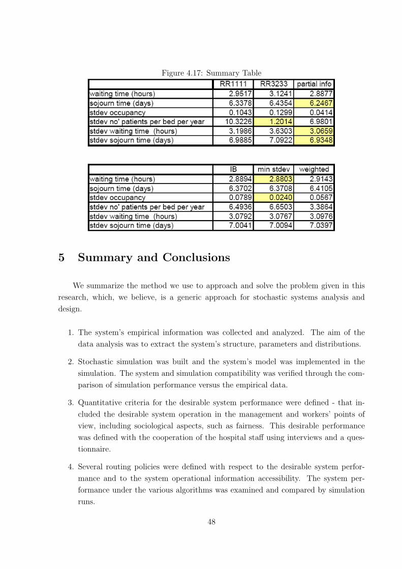
Figure 4.17: Summary Table
5 Summary and Conclusions
We summarize the method we use to approach and solve the problem given in this
research, which, we believe, is a generic approach for stochastic systems analysis and
design.
1. The system’s empirical information was collected and analyzed. The aim of the
data analysis was to extract the system’s structure, parameters and distributions.
2. Stochastic simulation was built and the system’s model was implemented in the
simulation. The system and simulation compatibility was verified through the com-
parison of simulation performance versus the empirical data.
3. Quantitative criteria for the desirable system performance were defined - that in-
cluded the desirable system operation in the management and workers’ points of
view, including sociological aspects, such as fairness. This desirable performance
was defined with the cooperation of the hospital staff using interviews and a ques-
tionnaire.
4. Several routing policies were defined with respect to the desirable system perfor-
mance and to the system operational information accessibility. The system per-
formance under the various algorithms was examined and compared by simulation
runs.
48

5. The planned but undone step in our work was to use some local or global optimality
search methods in order to adjust the algorithms’ parameters to achieve optimal
system performance (see Section 6).
Concluding remarks:
• The occupancy balancing method has shown (Section 4.3) very good performance, in
particular - low probability for overflow (little mass around ρ = 1), shorter waiting
and sojourn times, and balanced occupancy rates.
• However, the occupancy balancing algorithm tends to allocate more patients to the
fastest ward which is unfair to its staff. The flow balancing method is designed to
keep an equal number of patients per bed per year which is fairer but is “bad for
business”, in the sense of longer waits (best-performing policy will be to send more
patients to the fastest ward - see [1]).
• By adjusting the weights in the weighted algorithm, which combines the two pre-
viously mentioned methods, we can achieve system performance which will both
be fair for the staff, and maintain good operational performance. We assigned the
same importance to both methods ({α1, α2} = {0.5, 0.5}), but other weights can be
examined as well.
• Additionally we show that the occupancy balancing method may be implemented in
partial information access systems (one information update per day) with almost no
effect on the performance. The flow balancing method may be clearly implemented
in partial information access since it involves counting the routed patients with no
respect to ward occupancy.
• In summary, the proposed weighted algorithm achieves the best performance and
may be implemented in partial information access systems, which reduces the de-
mands on the design and implementation of the control system.
49
6 Limitations and Ideas for Future Research
When facing the task of modeling complex reality in limited time, we had to allow
relaxations and simplifying assumptions. Clearly, this hurt the accuracy of our results.
However, the created simulation tool is very generic and in future more details may be
added which will depict the process more accurately. Below is a list of the items we
simplified or omitted while building the model, and which can be added and investigated
in further research:
• Different patient categories: As we mentioned earlier, when arriving to the
ED, patients are classified as “walking” and “lying”. In addition, prior to running
the Justice Table they are classified as “regular”, “special care” or “ventilated”.
The load, inflicted on the hospital by patients, varies significantly among different
categories: in LOS, complexity of treatment and waiting times. In our simulation all
patients are the same, describing an “average” patient - this simplifies the routing
and scheduling process, but presents a limitation as well.
• Returning patients: Those are patients who return to the IW’s within a month
from their previous hospitalization there. Such patients present about 14 percent of
all the admissions ([8]) and mostly are placed in the same ward in which they were
hospitalized previously (unless they object to it). Accounting for returning patients
in the routing process will make the simulation closer to reality, and might affect
the results.
• ED modeling: As our goal is to simulate the interface between the ED and the
IW, the simulation begins from the point of hospitalization decision. Thus it does
not show the influence of long waiting times on the ED resources: beds and staff.
Integrating our simulation with the ED simulation tool created by [15] will allow a
better understanding of the whole complex picture.
• Ward E: Ward E differs significantly from the other wards by the type of patients
hospitalized there (only walking , independent patients), turnover rate (more admis-
sions and discharges per day), number of patients treated by one nurse/physician.
Thus routing to Ward E is not done via the Justice Table, and we excluded it
from our study. Nevertheless, it might be interesting to study more deeply fairness
aspects concerning Ward E and present routing algorithms that will include it as
well.
• LOS accounting for routing policies: We model the LOS invariant to different
routing policies, while in reality they certainly might change, as some policies provide
50

incentives to wards to discharge patients quicker and others - the opposite. As well
there may exist a connection between LOS and the load the ward is subjected
to - for example, [7] found that in cardiothoracic surgery workers accelerated the
service rate as load increased. An interesting point for future research might be to
investigate such possible connection in our case and model it in the simulation.
• Waiting times modeling: We modeled waiting times in a quite simple and in-
tuitive way (see Section 2.1), which was not supported by quantitative empirical
data (due to lack of such). By conducting observations in the ED, one can measure
waiting times and try to model them as a function of the load on the wards. “Load”
in its turn, can be defined differently than just the percentage of occupied bed: for
example, account as well for the number of recent admissions and discharges, and
severity of hospitalized patients. In addition, there is a significant psychological fac-
tor in determining waiting times - much of the decisions of where and when to place
a patient are made through internal politics and personal communications between
nurses - which makes modeling waiting times task quite challenging.
• Sensitivity analysis: All the parameters required for a simulation were estimated
based on data from the information systems in Rambam. Needless to say that such
data is not one hundred percent reliable, as it might be subjected to human mistakes
and inaccuracy. As well mistakes may occur during data analysis. Thus one should
perform a sensitivity analysis: test what happens to simulation results when arrival
rate, LOS or waiting times change.
• Optimal search and heuristics: As we mentioned in Section 4.3, in our weighted
algorithm implementation we chose to use equal weights to both of the criteria
({α1, α2} = {0.5, 0.5}). It can be seen that any choice of weight proportions will
give different importance to each of the criteria, and may change the system per-
formance. One can expand our work by using local optimization search methods,
as gradient descent or Newton’s method, in order to find the weight proportions
which give maximum value to some grade function that represents desirable system
performance. Another approach may be to use global optimization search heuristics
as Cross-Entropy and Genetic algorithm.
• Reinforcement Learning (RL): Reinforcement Learning is concerned with vari-
ous methods which enable computers to “learn”. The purpose of the method is to
find a policy that maximizes the expected return - in our terminology this method
may find the routing policy which maximizes the desirable system performance.
During the “learning” process the agent interacts with the environment by a trial
and error search (exploration-exploitation) in order to identify regularities in the
51

rewards received (performance grade function) for the current state and action. RL
operation structure can be viewed in the figure below:
The specific implementation method usually consists of recursive use of Bellman Opti-
mality Equation, as in the Q-learning method described below.
Let us define the following notations:
• xt - system state at time t. In our case it can be {ρi(t), γi(t)} for all i ∈ {1, . . . , 4} .
• at - recommended action at state xt. In our case it is the routing decision (which is
the station index).
• Qt(xt, at)- value function for state xt and action at.
• γ- capitalize value parameter, we demand γ < 1.
• α- stochastic approximation parameter which is needed to ensure convergence of the
iterative calculation in the case of noisy estimation (or any other random sampling).
We demand that α fulfill the following requirements:
1.∞∑i=1
α2 < ∞
2.∞∑i=1
α = ∞
Now our iterative value function is estimated as follows:Qt+1(xt, at) = (1− α) ·Qt(xt, at) + α · [rt + γ ·maxa′ (Qt(xt+1, a
′))];
Qt+1(x, a) = Qt(x, a) ∀(x, a) 6= (xt, at);
(6.1)
52

After convergence of Q(x, a) (we do not define here the convergence criterion), we calculate
the optimal routing policy:
π∗(x) = argmaxa{Q(x, a)} (6.2)
53
References
[1] M. Armony, Dynamic routing in large-scale service systems with heterogeneous
servers, Queueing Systems 51 (2005), 287–329. 1.3, 5
[2] M. Armony and A. Ward, Fair dynamic routing policies in large-scale systems with
heterogeneous servers, Manuscript under review. 1.3
[3] B. Avi-Itzhak and H. Levy, Measuring fairness in queues, Advances in Applied Prob-
ability 36 (2004), 919–936. 1.3, 4.1
[4] R. Bekker and A.M. de Bruin, Time-dependent analysis for refused admissions in
clinical wards, Submitted to AOR-ORAHS’s special volume (2008). 1.3, 2.1
[5] M. Ben-Zrihen, J. Borsher, A. Reiss, and Y. Tseytlin, Behavioral models in customer
service centers, IE&M Undergraduate Project, Technion (2007). 1.3
[6] A.B. Cooper, E. Litvak, M.C. Long, and M.L. McManus, Emergency department
diversion: causes and solutions, Academic Emergency Medicine 8 (2001), 1108–1110.
1.3
[7] K.C. Diwas and C. Terwiesch, The impact of work load on productivity and quality:
an econometric analysis of hospital operations, Manuscript under review (2008). 1.3,
6
[8] K. Elkin and N. Rozenberg, Patients’ flow from the emergency department to the
internal wards, IE&M Undergraduate Project, Technion (2007). 1, 1.2, 1.2, 2.1, 2.1,
4.1, 6
[9] P. Gonzales and C. Herrero, Optimal sharing of surgical costs in the presence of
queues, Mathematical Methods of Operations Research 59 (2004), 435–446. 1.3
[10] L. Green, Capacity planning and management in hospitals, Operations Research and
Health Care (Brandwau et al editors) (2004), 14–41. 1.3
[11] , Using operations research to reduce delays for healthcare, Tutorials in Oper-
ations Research, Informs (2008). 1.3
[12] R.C. Huseman, J.D. Hatfield, and E.W. Miles, A new perspective on equity theory:
the equity sensitivity construct, The Academy of Management Review 12 (1987),
no. 2, 222–234. 1.3
[13] O.B. Jennings and F.d. Vericourt, Nurse-to-patient ratios in hospital staffing: a queu-
ing perspective, Working Paper, Duke University. 1.3, 2.1
54

[14] R.C. Larson, Perspectives on queues: social justice and the psychology of queueing,
Operations Research 35 (1987), 895–905. 1.3
[15] Y. Marmor and D. Sinreich, Emergency departments operations: the basis for de-
veloping a simulation tool, IIE Transactions 37 (2005), no. 3, 233–245. 1.3, 2.1,
6
[16] Rambam Hospital: Report of the Quality Promotion Team, Reducing waiting times
in the emergency department and los in the internal wards, (1997). 1.2
[17] A. Rafaeli, G. Barron, and K. Haber, The effects of queue structure on attitudes,
Journal of Service Research 5 (2002), no. 2, 125–139. 1.3
[18] M.J. Soomer and G.M. Koole, Fairness in the aircraft landing problem, Working
paper. 4.1
[19] T. Tezcan, Optimal control of distributed parallel server systems under the halfin and
whitt regime, Math of OR (2007). 1.3
55

APPENDIX
A Routing Process Flow Charts
Figure A.1: Activities Flow Chart
Hospitalization decision
Assigning Ward (A-D) with the Justice Table
Ward requests skipping
Transferal time decision
Patient’s status updating
Management approves skipping
Bed preparation
Yes
No
Yes
No
Initial measurements collection
Transferal to the Ward
Initial physician check
Coordination with medical staff
Ventilated patient?
No
YesCoordination with medical staff in
the ED
“Walking” patient? Yes
No
Assigned to Ward E
* Processes in broken line occur in the IW
- Ending point of simultaneous processes
Ward E
Wards A-D
Bed preparationWard E
56

Figure A.2: Resources Flow Chart
Resource Queue - Synchronization Queue -
ED physician
ED nurse in chargeReceptionist IW nurse in
charge
General Nurse
IW physicianStretcher Bearer
Help forceIW nurse
Allocation
Skippingrequest
Ventilated patient
- Ending point of simultaneous processes
Transferal
Measurements
Medical check
Coordination
57

Figure A.3: Information Flow Chart
ED medical file
ED physician
Type (regular, special care, ventilated)
ED nurse in charge
Allocation: Ward A-D
Receptionist
Transfer time
IW nurse in charge
Skipping granted/ not granted
General nurse
Skipping request + reasons
IW nurse in charge
Patient’s status updating
ED nurse in charge
Type + medical information
ED nurse in charge
Preparation for patient’s admission
IW nurse in charge
Medical check results
IW physician
Initial measurements results
IW nurse in charge
Availability check
Bed readiness check
Help force
Clinical information
ED physician
Ventilatedpatient
Transfer time updating
ED nurse in charge
Availability check
- Ending point of simultaneous processes
Availability check
ED physician or nurse
Ventilatedpatient
Ventilatedpatient
IW nurse
IW physician
58

B Arrivals and LOS Empirical Data Analysis
Figure B.1: Compatibility of Arrivals Distribution to Poisson - Sunday
Distribution Summary Distribution: Poisson Expression: POIS(24) Square Error: 0.006938 Chi Square Test Number of intervals = 14 Degrees of freedom = 12 Test Statistic = 25.2 Corresponding p-value = 0.0151 Data Summary Number of Data Points = 200 Min Data Value = 10 Max Data Value = 42 Sample Mean = 24 Sample Std Dev = 5.31 Histogram Summary Histogram Range = 9.5 to 42.5 Number of Intervals = 33
59

Figure B.2: Compatibility of LOS distribution to Log-Normal - Ward A
Distribution Summary
Distribution: Lognormal
Expression: LOGN (6.92, 7.65)
Square Error: 0.003063
Chi Square Test
Number of intervals = 15
Degrees of freedom = 12
Test Statistic = 94.4
Corresponding p-value < 0.005
Kolmogorov-Smirnov Test
Test Statistic = 0.0487
Corresponding p-value < 0.01
Data Summary
Number of Data Points = 7254
Min Data Value = 0.01
Max Data Value = 152
Sample Mean = 6.85
Sample Std Dev = 7.62
Histogram Summary
Histogram Range = 0 to 152
Number of Intervals = 40
60