SIMULATION OF PARTICLE AGGLOMERATION USING

DISSIPATIVE PARTICLE DYNAMICS

A Thesis

by

SRINIVAS PRAVEEN MOKKAPATI

Submitted to the Office of Graduate Studies ofTexas A&M University

in partial fulfillment of the requirements for the degree of

MASTER OF SCIENCE

December 2006

Major Subject: Mechanical Engineering

SIMULATION OF PARTICLE AGGLOMERATION USING

DISSIPATIVE PARTICLE DYNAMICS

A Thesis

by

SRINIVAS PRAVEEN MOKKAPATI

Submitted to the Office of Graduate Studies ofTexas A&M University

in partial fulfillment of the requirements for the degree of

MASTER OF SCIENCE

Approved by:

Chair of Committee, Arun R. SrinivasaCommittee Members, Anastasia H. Muliana

Tahir CaginHead of Department, Dennis O’Neal

December 2006

Major Subject: Mechanical Engineering

iii

ABSTRACT

Simulation of Particle Agglomeration Using

Dissipative Particle Dynamics. (December 2006)

Srinivas Praveen Mokkapati, B.E., Osmania University

Chair of Advisory Committee: Dr. Arun R Srinivasa

Attachment of particles to one another due to action of certain inter-particle

forces is called as particle agglomeration. It has applications ranging from efficient

capture of ultra-fine particles generated in coal-burning boilers to effective discharge

of aerosol sprays. Aerosol sprays have their application in asthma relievers, coat-

ings, cleaning agents, air fresheners, personal care products and insecticides. There

are several factors that cause particle agglomeration and based on the application,

agglomeration or de-agglomeration is desired. These various factors associated with

agglomeration include van der Waals forces, capillary forces, electrostatic double-layer

forces, effects of turbulence, gravity and brownian motion. It is therefore essential

to understand the underlying agglomeration mechanisms involved. It is difficult to

perform experiments to quantify certain effects of the inter-particle forces and hence

we turn to numerical simulations as an alternative. Simulations can be performed

using the various numerical simulation techniques such as molecular dynamics, dis-

crete element method, dissipative particle dynamics or other probabilistic simulation

techniques.

The main objective of this thesis is to study the geometric characteristics of par-

ticle agglomerates using dissipative particle dynamics. In this thesis, agglomeration

is simulated using the features of dissipative particle dynamics as the simulation tech-

nique. Forces of attraction from the literature are used to modify the form of the

conservative force. Agglomeration is simulated and the characteristics of the result-

iv

ing agglomerates are quantified. Simulations were performed on a sizeable number

of particles and we observe agglomeration behavior. A study of the agglomerates

resulting from the different types of attractive forces is performed to characterize

them methodically. Also as a part of this thesis, a novel, dynamic particle simulation

technique was developed by interfacing MATLAB and our computational C program.

v

To Almighty and my parents, Padmavathy and Prabhakara

vi

ACKNOWLEDGMENTS

I shall remain indebted to many people throughout my graduate study at Texas

A&M for their very presence and for having given me constant encouragement,

morally and academically. I’d like to appreciate all such people and even though

some might not find a mention here, I thank them sincerely for everything.

I’d like to express my gratitude to my advisor, Dr. Arun R. Srinivasa for his

steadfast encouragement and constant support. Certainly, the amount of patience he

had for me was immeasurable. Only I know how much he supported me towards the

latter stages of my Master’s degree. I shall remain thankful to him for everything that

he has done for me. I also wish to extend my gratitude to the rest of my committee

members. Learning from Dr. Tahir Cagin was a great experience for me and I thank

him for providing me with one. Also, I thank Dr. Anastasia Muliana for serving on

my committee.

I’d like thank a couple of people without whose support I wouldn’t have achieved

this. I’d like to express my heartfelt gratitude to A.S.Nandagopalan for the friendship

we shared over the past couple of years. I shall remain grateful to him for the person

he is and for the many things that I learned from him to be a better person. I’d like

to thank Harini Gudi for being an amazing friend and for her cheerful countenance

which is always a welcome relief. I express to her my appreciation also for the constant

words of support and encouragement. Thank you both.

I thank Anshul Kaushik for his constant guidance and insightful remarks during

my research over the past year and also for his infectious liveliness. Also, my thanks

to Saradhi Koneru for his constant support on the academic front and for being a

good friend. My sincere thanks to Raghuveer Sharma and Sajjan Bollu for their

amazing friendship as my life here would have been mundane without their presence.

vii

Also, I wish to thank the many people and friends who have been around my life

here at Texas A&M. For their companionship and for having given me newer insights

in various aspects, I’d like to thank Chinmay Deshpande, Nipun Sinha, Vijaykumar

Sathyamurthi, Seemant Yadav, Sukesh Shenoy, Satish Karra and my other friends

from my batch, previous batch and the succeeding batch.

Finally, any amount of words spoken about my family here would just be an

understatement. However, I wish to appreciate my parents for their constant support

and words of wisdom at every crucial juncture of my life. The love and trust that

they have for me is unfathomable. Thank you.

viii

TABLE OF CONTENTS

CHAPTER Page

I INTRODUCTION . . . . . . . . . . . . . . . . . . . . . . . . . . 1

A. Introduction . . . . . . . . . . . . . . . . . . . . . . . . . . 1

B. Applications . . . . . . . . . . . . . . . . . . . . . . . . . . 1

C. Agglomeration Mechanisms . . . . . . . . . . . . . . . . . 3

1. van der Waals attraction . . . . . . . . . . . . . . . . 4

2. Capillary forces . . . . . . . . . . . . . . . . . . . . . . 6

3. Electrostatic agglomeration . . . . . . . . . . . . . . . 6

4. Brownian agglomeration . . . . . . . . . . . . . . . . . 7

5. Gravitational agglomeration . . . . . . . . . . . . . . . 8

6. Turbulent agglomeration . . . . . . . . . . . . . . . . 9

D. Possible Approaches . . . . . . . . . . . . . . . . . . . . . 10

1. Molecular Dynamics . . . . . . . . . . . . . . . . . . . 11

2. Discrete Element Method . . . . . . . . . . . . . . . . 12

3. Dissipative Particle Dynamics . . . . . . . . . . . . . . 12

4. Lattice Boltzmann Method . . . . . . . . . . . . . . . 13

5. Monte Carlo Methods . . . . . . . . . . . . . . . . . . 14

6. Lattice Gas Automata . . . . . . . . . . . . . . . . . . 15

E. Past Work in Agglomeration . . . . . . . . . . . . . . . . . 15

II SCOPE AND OBJECTIVES . . . . . . . . . . . . . . . . . . . . 18

A. Scope . . . . . . . . . . . . . . . . . . . . . . . . . . . . . . 18

B. Objectives . . . . . . . . . . . . . . . . . . . . . . . . . . . 18

III DISSIPATIVE PARTICLE DYNAMICS: DESCRIPTION AND

REQUIREMENTS OF OUR PROBLEM . . . . . . . . . . . . . 20

A. Theory . . . . . . . . . . . . . . . . . . . . . . . . . . . . . 20

B. Salient Features . . . . . . . . . . . . . . . . . . . . . . . . 20

C. Time Integration Schemes . . . . . . . . . . . . . . . . . . 22

1. Euler scheme . . . . . . . . . . . . . . . . . . . . . . . 23

2. Verlet scheme . . . . . . . . . . . . . . . . . . . . . . . 23

3. Velocity Verlet scheme . . . . . . . . . . . . . . . . . . 24

4. Predictor Corrector scheme . . . . . . . . . . . . . . . 24

5. Leap Frog scheme . . . . . . . . . . . . . . . . . . . . 24

ix

CHAPTER Page

6. Beeman algorithm . . . . . . . . . . . . . . . . . . . . 25

7. Dissipative Particle Dynamics - Velocity Verlet algorithm 25

D. Boundary Conditions . . . . . . . . . . . . . . . . . . . . . 25

E. Past Work in DPD and Its Applications . . . . . . . . . . 26

F. Requirements, Constraints and Approach of Simulation . . 30

1. MEX . . . . . . . . . . . . . . . . . . . . . . . . . . . 30

2. Writing MEX-files . . . . . . . . . . . . . . . . . . . . 31

3. MEX and its application to our requirements . . . . . 32

4. Dynamic Simulation . . . . . . . . . . . . . . . . . . . 32

IV APPROACH . . . . . . . . . . . . . . . . . . . . . . . . . . . . . 33

A. Modified Features of DPD . . . . . . . . . . . . . . . . . . 33

B. Non-dimensionalization of Units . . . . . . . . . . . . . . . 37

C. Algorithm . . . . . . . . . . . . . . . . . . . . . . . . . . . 39

D. Characterizing Agglomerates . . . . . . . . . . . . . . . . . 40

V RESULTS AND CONCLUSIONS . . . . . . . . . . . . . . . . . 43

A. Parameters in Computations . . . . . . . . . . . . . . . . . 43

B. Results . . . . . . . . . . . . . . . . . . . . . . . . . . . . . 44

C. Analysis . . . . . . . . . . . . . . . . . . . . . . . . . . . . 46

REFERENCES . . . . . . . . . . . . . . . . . . . . . . . . . . . . . . . . . . . 53

APPENDIX A . . . . . . . . . . . . . . . . . . . . . . . . . . . . . . . . . . . 58

APPENDIX B . . . . . . . . . . . . . . . . . . . . . . . . . . . . . . . . . . . 62

VITA . . . . . . . . . . . . . . . . . . . . . . . . . . . . . . . . . . . . . . . . 63

x

LIST OF TABLES

TABLE Page

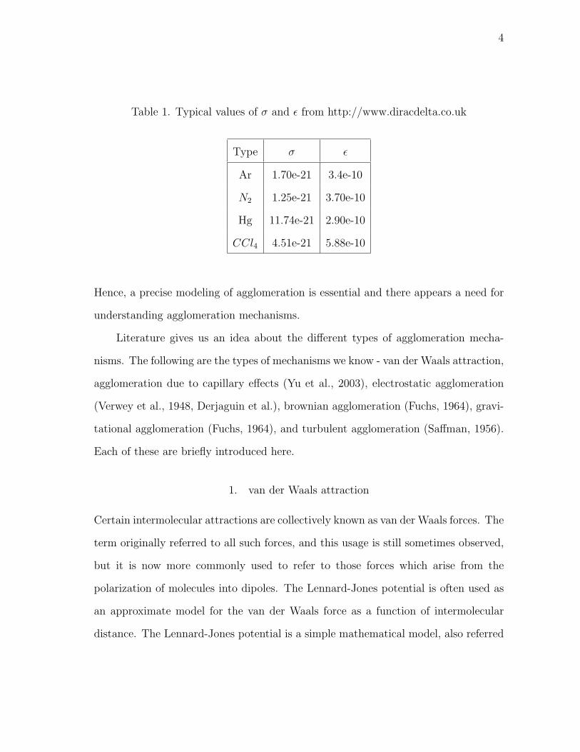
1 Typical values of σ and ε from http://www.diracdelta.co.uk . . . . . 4

2 Classification of ellipsoids . . . . . . . . . . . . . . . . . . . . . . . . 47

3 Classification of ellipsoids for van der Waals forces . . . . . . . . . . 48

4 Volume of ellipsoids as a % (average) of volume of individual par-

ticles put together for van der Waals forces . . . . . . . . . . . . . . 48

5 Classification of ellipsoids for capillary forces . . . . . . . . . . . . . . 50

6 Volume of ellipsoids as a % (average) of volume of individual par-

ticles put together for capillary forces . . . . . . . . . . . . . . . . . . 51

xi

LIST OF FIGURES

FIGURE Page

1 Image Courtesy: EPA Website (http://www.epa.gov) . . . . . . . . . 2

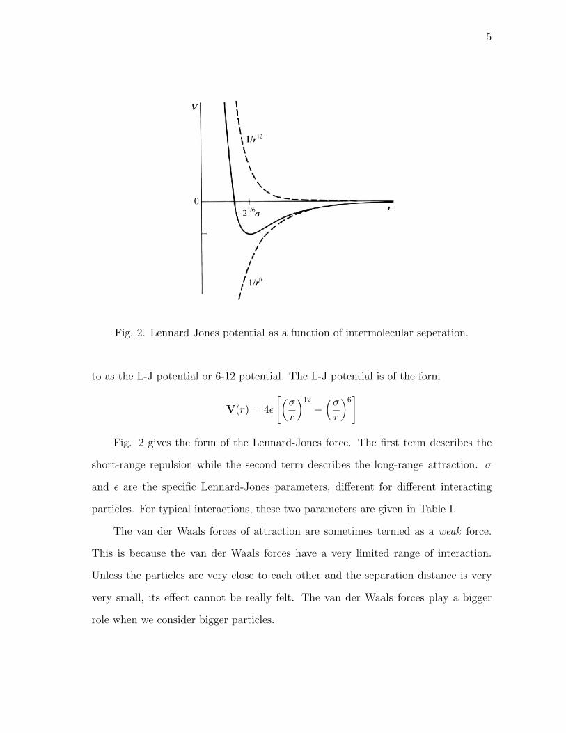
2 Lennard Jones potential as a function of intermolecular seperation. . 5

3 Schematic of the free energy with particle separation according to

DLVO theory. . . . . . . . . . . . . . . . . . . . . . . . . . . . . . . . 7

4 Example of Brownian motion of a particle. . . . . . . . . . . . . . . . 8

5 Schematic of gravitational agglomeration. . . . . . . . . . . . . . . . 9

6 Schematic of two types of turbulent agglomeration (a) Shear Ag-

glomeration, (b) Inertial Agglomeration . . . . . . . . . . . . . . . . 10

7 Use of Monte Carlo to evaluate the value of π . . . . . . . . . . . . . 14

8 Simple schematic of an Electrostatic Precipitator . . . . . . . . . . . 16

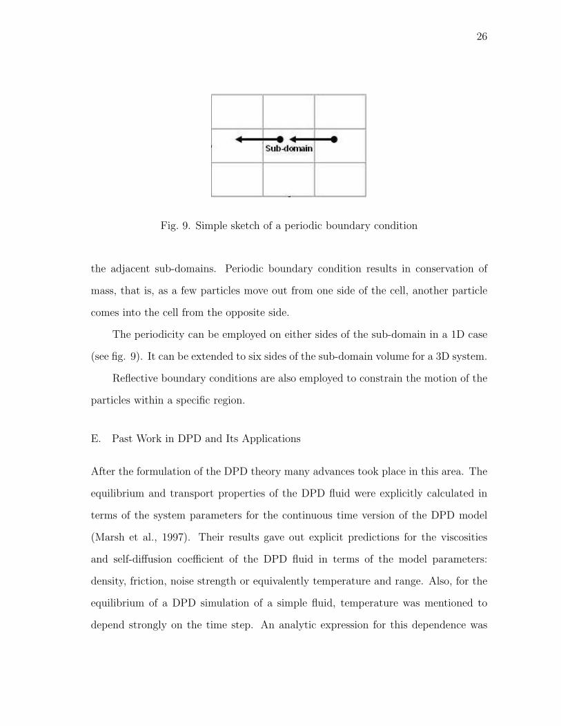
9 Simple sketch of a periodic boundary condition . . . . . . . . . . . . 26

10 Plot of F/F0 vs. r/rc . . . . . . . . . . . . . . . . . . . . . . . . . . . 34

11 Schematic of a liquid bridge formation near spheres’ vicinity . . . . . 36

12 Flowchart of approach . . . . . . . . . . . . . . . . . . . . . . . . . . 38

13 Types of agglomerates . . . . . . . . . . . . . . . . . . . . . . . . . . 40

14 Shape of a typical prolate ellipsoid (a > b = c) . . . . . . . . . . . . . 41

15 A typical Maxwell - Boltzmann distribution. . . . . . . . . . . . . . . 44

16 Clusters showing the formation of agglomerates. . . . . . . . . . . . . 45

17 Individual clusters. . . . . . . . . . . . . . . . . . . . . . . . . . . . . 45

18 Ellipsoids depicting the clusters . . . . . . . . . . . . . . . . . . . . . 46

xii

FIGURE Page

19 Distribution of volume of ellipsoids for van der Waals forces . . . . . 49

20 Distribution of volume of ellipsoids for capillary forces . . . . . . . . 51

1

CHAPTER I

INTRODUCTION

A. Introduction

Agglomeration is a process in which the particles collide and stick with each other

forming dendritic structures. Upon collision, if the particles coalesce into each other,

it is referred to as coagulation, which is a special case of agglomeration. A simple

explanation of the process of agglomeration is due to minimization of energy. If two

particles come closer and stick to each other or even proceed to coalesce, the net

surface energy would decrease. This is a natural tendency to agglomerate. However,

there might be particles such as particles of same polarity which will not agglomerate

under normal conditions. It may have important consequences for particle transport

as larger agglomerates are affected more by gravity and they diffuse slowly.

The agglomeration of particles has several applications in the industrial world.

A few of them are briefly mentioned in the following section.

B. Applications

Since the past decades, there has been increase in the production of finer particles,

need for efficient collection of these fine particles present in flue gases, undesired

accumulation of matter, etc. The list of its ever-growing applications cannot be

exhausted here. However, the following is a list of few of its industrial applications:

1. Boilers that are fueled by coal produce flue gases which contain harmful ultra-

fine particles. These fine particles are capable of entering the human respiratory

The journal model is International Journal of Applied Mechanics and Engineering.

2

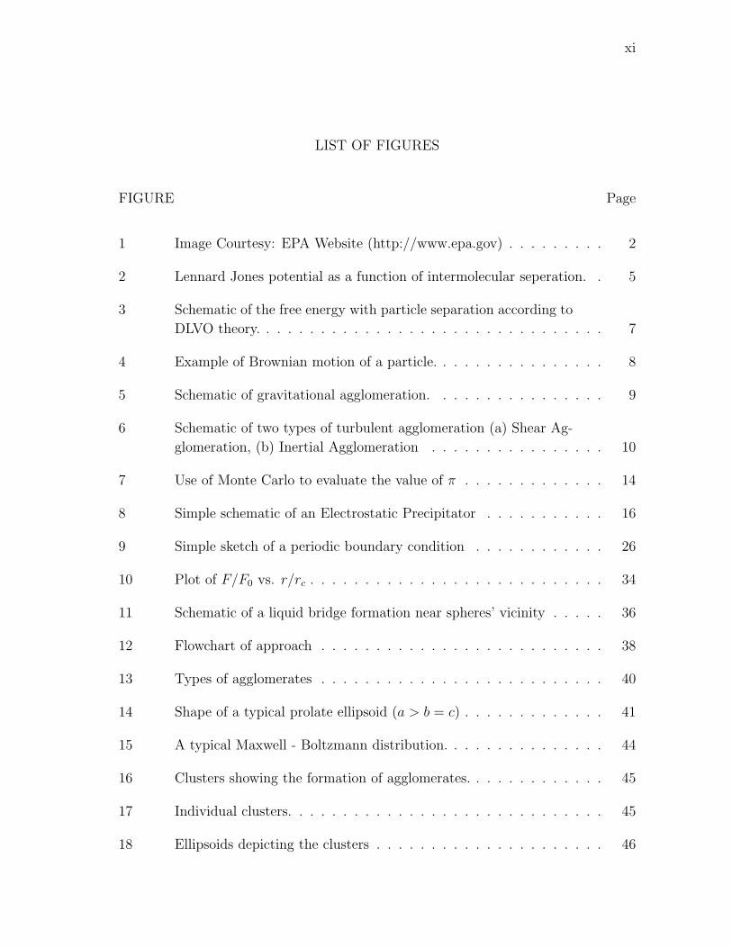
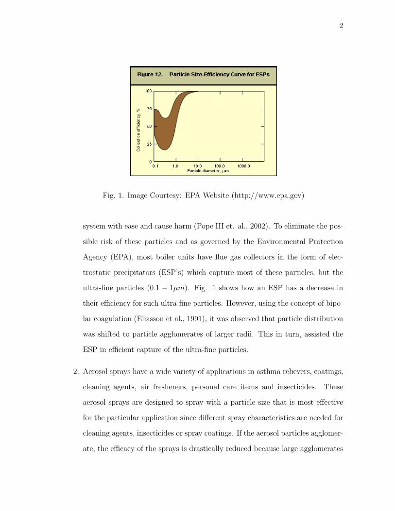
Fig. 1. Image Courtesy: EPA Website (http://www.epa.gov)

system with ease and cause harm (Pope III et. al., 2002). To eliminate the pos-

sible risk of these particles and as governed by the Environmental Protection

Agency (EPA), most boiler units have flue gas collectors in the form of elec-

trostatic precipitators (ESP’s) which capture most of these particles, but the

ultra-fine particles (0.1 − 1µm). Fig. 1 shows how an ESP has a decrease in

their efficiency for such ultra-fine particles. However, using the concept of bipo-

lar coagulation (Eliasson et al., 1991), it was observed that particle distribution

was shifted to particle agglomerates of larger radii. This in turn, assisted the

ESP in efficient capture of the ultra-fine particles.

2. Aerosol sprays have a wide variety of applications in asthma relievers, coatings,

cleaning agents, air fresheners, personal care items and insecticides. These

aerosol sprays are designed to spray with a particle size that is most effective

for the particular application since different spray characteristics are needed for

cleaning agents, insecticides or spray coatings. If the aerosol particles agglomer-

ate, the efficacy of the sprays is drastically reduced because large agglomerates

3

offer greater resistance to flow and their tendency to diffuse reduces.

3. Medicinal applications include dry powder inhaler (one common inhaler for

asthma), which should possess a quick and efficient drug delivery process for

an asthma patient’s lungs upon its use. Upon inhalation, the aerosolized pow-

ders must be in a sufficiently de-agglomerized state for better and quick results.

Also, we have agglomeration in the form of tablets, lozenges, etc. The manu-

facture of the medicinal tablets is by wetting the fine medicine particles with

an appropriate liquid, and by the action of capillary forces these fine particles

agglomerate.

4. In chemical industries, we can see the applications of agglomerates in the manu-

facture of laundry detergents, pigments, and biocides (chemical used for sanitiz-

ing water). Food industry applications include artificial sweeteners, coffee and

tea powders and pudding mixes. Animal and fish feeds, which are in the form of

pellets, are manufactured using agglomeration. Same is the case with fertilizer

granules, iron ore pellets, and briquettes (used as melt charge for furnaces).

C. Agglomeration Mechanisms

This field of study has gained importance in the recent past due to the increased

manufacture, use and after-effects of the fine particles along with a commensurate

understanding of particle behavior in the microscopic scale. In some of the above

mentioned applications, there is a need for agglomerating fine particles. While in

the case of larger agglomerates, due to the greater mass, more resistance to particle

transport is offered and more effort to overcome that resistance is required. As a

result, if there is a proper understanding of these agglomerates and their behavior

towards de-agglomeration, design of their transport mechanisms can be optimized.

4

Table 1. Typical values of σ and ε from http://www.diracdelta.co.uk

Type σ ε

Ar 1.70e-21 3.4e-10

N2 1.25e-21 3.70e-10

Hg 11.74e-21 2.90e-10

CCl4 4.51e-21 5.88e-10

Hence, a precise modeling of agglomeration is essential and there appears a need for

understanding agglomeration mechanisms.

Literature gives us an idea about the different types of agglomeration mecha-

nisms. The following are the types of mechanisms we know - van der Waals attraction,

agglomeration due to capillary effects (Yu et al., 2003), electrostatic agglomeration

(Verwey et al., 1948, Derjaguin et al.), brownian agglomeration (Fuchs, 1964), gravi-

tational agglomeration (Fuchs, 1964), and turbulent agglomeration (Saffman, 1956).

Each of these are briefly introduced here.

1. van der Waals attraction

Certain intermolecular attractions are collectively known as van der Waals forces. The

term originally referred to all such forces, and this usage is still sometimes observed,

but it is now more commonly used to refer to those forces which arise from the

polarization of molecules into dipoles. The Lennard-Jones potential is often used as

an approximate model for the van der Waals force as a function of intermolecular

distance. The Lennard-Jones potential is a simple mathematical model, also referred

5

Fig. 2. Lennard Jones potential as a function of intermolecular seperation.

to as the L-J potential or 6-12 potential. The L-J potential is of the form

V(r) = 4ε

[(σ

r

)12

−(

σ

r

)6]

Fig. 2 gives the form of the Lennard-Jones force. The first term describes the

short-range repulsion while the second term describes the long-range attraction. σ

and ε are the specific Lennard-Jones parameters, different for different interacting

particles. For typical interactions, these two parameters are given in Table I.

The van der Waals forces of attraction are sometimes termed as a weak force.

This is because the van der Waals forces have a very limited range of interaction.

Unless the particles are very close to each other and the separation distance is very

very small, its effect cannot be really felt. The van der Waals forces play a bigger

role when we consider bigger particles.

6

2. Capillary forces

Capillarity is a phenomenon which we see in our daily lives. The supply of water

from the soil to the plants is due to capillarity. The absorption of water due to

paper towels or sponges is again due to capillarity. In applications where we have

wet particles interacting with each other, the capillary forces play a very important

role in agglomeration. The adhesive intermolecular forces between the particles cause

the particles to stick to each other. The cohesive intermolecular forces try to reduce

the surface tension. Due to the presence of wetness, the adhesive forces are stronger

than the cohesive forces causing the particles to agglomerate. The capillary force is

a function of surface tension, the radii of the particles under consideration and the

inter-particle separation. Previously, work has been done to quantify porosity and the

capillary forces acting on wet particles (Yu et al., 2003). In their work, an equation

was developed to describe the general relationship between porosity of packed particles

and inter-particle forces. This was based on experimental observations of porosity

dependence on particle size and inter-particle forces. Their work used van der Waals

and capillary forces on 11000 micron sized particles.

3. Electrostatic agglomeration

This has been studied using the DVLO Theory which is named after Deryaguin,

Landau, Verwey and Overbeek (Verwey et al., 1948, Derjaguin et al.). This has

been established since the 1940’s and shown to apply successfully to a wide range of

colloidal systems. According to this theory, there are two forces in a solution namely,

electrostatic repulsion force which repels approaching particles and the attractive van

der Waals which binds the particles together. This is valid only for special type

of solutions called stabilized solutions, which are characterized by all the particles

7

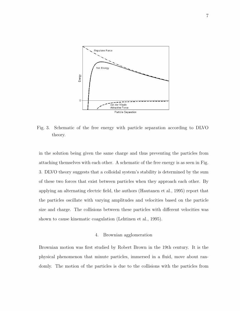
Fig. 3. Schematic of the free energy with particle separation according to DLVO

theory.

in the solution being given the same charge and thus preventing the particles from

attaching themselves with each other. A schematic of the free energy is as seen in Fig.

3. DLVO theory suggests that a colloidal system’s stability is determined by the sum

of these two forces that exist between particles when they approach each other. By

applying an alternating electric field, the authors (Hautanen et al., 1995) report that

the particles oscillate with varying amplitudes and velocities based on the particle

size and charge. The collisions between these particles with different velocities was

shown to cause kinematic coagulation (Lehtinen et al., 1995).

4. Brownian agglomeration

Brownian motion was first studied by Robert Brown in the 19th century. It is the

physical phenomenon that minute particles, immersed in a fluid, move about ran-

domly. The motion of the particles is due to the collisions with the particles from

8

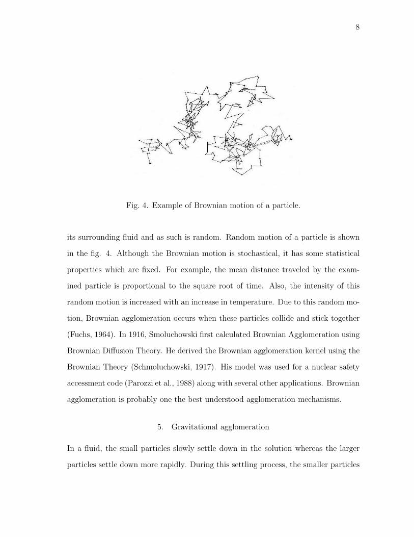
Fig. 4. Example of Brownian motion of a particle.

its surrounding fluid and as such is random. Random motion of a particle is shown

in the fig. 4. Although the Brownian motion is stochastical, it has some statistical

properties which are fixed. For example, the mean distance traveled by the exam-

ined particle is proportional to the square root of time. Also, the intensity of this

random motion is increased with an increase in temperature. Due to this random mo-

tion, Brownian agglomeration occurs when these particles collide and stick together

(Fuchs, 1964). In 1916, Smoluchowski first calculated Brownian Agglomeration using

Brownian Diffusion Theory. He derived the Brownian agglomeration kernel using the

Brownian Theory (Schmoluchowski, 1917). His model was used for a nuclear safety

accessment code (Parozzi et al., 1988) along with several other applications. Brownian

agglomeration is probably one the best understood agglomeration mechanisms.

5. Gravitational agglomeration

In a fluid, the small particles slowly settle down in the solution whereas the larger

particles settle down more rapidly. During this settling process, the smaller particles

9

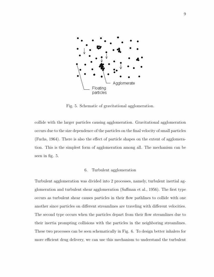
Fig. 5. Schematic of gravitational agglomeration.

collide with the larger particles causing agglomeration. Gravitational agglomeration

occurs due to the size dependence of the particles on the final velocity of small particles

(Fuchs, 1964). There is also the effect of particle shapes on the extent of agglomera-

tion. This is the simplest form of agglomeration among all. The mechanism can be

seen in fig. 5.

6. Turbulent agglomeration

Turbulent agglomeration was divided into 2 processes, namely, turbulent inertial ag-

glomeration and turbulent shear agglomeration (Saffman et al., 1956). The first type

occurs as turbulent shear causes particles in their flow pathlines to collide with one

another since particles on different streamlines are traveling with different velocities.

The second type occurs when the particles depart from their flow streamlines due to

their inertia prompting collisions with the particles in the neighboring streamlines.

These two processes can be seen schematically in Fig. 6. To design better inhalers for

more efficient drug delivery, we can use this mechanism to understand the turbulent

10

Fig. 6. Schematic of two types of turbulent agglomeration (a) Shear Agglomeration,

(b) Inertial Agglomeration

shear forces that are responsible for breaking down of powdered drug agglomerates.

Since turbulence modeling is fraught with difficulties, this mechanism is the least

understood among the four.

D. Possible Approaches

There are many possible approaches to model our problem. To study particle agglom-

eration in which the length scales are microscopic, discrete microscopic/mesoscopic

models can be used effectively to simulate such systems’ behavior. Several models

over the past have been successfully employed for particle simulations. We will briefly

look at a few of the existing particle simulation models and/or approaches. Basically,

we can broadly classify these approaches into two types - Deterministic approaches

and Stochastic approaches.

Deterministic approaches have the ability to pin point particle positions and

velocities at any time using the Newton’s laws of motion. They include, but not

11

limited to, Molecular Dynamics, Discrete Element method and Dissipative Particle

Dynamics.

1. Molecular Dynamics

Molecular Dynamics (MD), first introduced by Alder and Wainwright in the late 50’s

(Alder et al., 1959) , captures the minute details of the interactions between the

particles by using Newton’s equations of motion on an atomistic scale. Since then,

this field has grown tremendously. The method of MD gained popularity in material

science and since the 70’s. The first molecular dynamics simulation of a real system

was simulation of liquid water in 1974 (Stillinger et al., 1974). Many advances have

taken place thereafter. For instance, a new feature of internal molecular temperature

was developed by the authors (Srinivasa et al., 2004).

In MD, the time duration of the simulation is dependent on the length of each

timestep, between which forces are recalculated. The timestep must be small so as

to avoid discretization errors. To capture a macroscopic effect using MD will require

a large number of time steps. This usually takes a lot of simulation time. To solve

this issue to some extent, parallel processing had been invented and used effectively

(Hendrickson et al., 1995, Plimpton, 1995) . In parallel processing, the task at hand

is split up and executed on multiple processors to obtain the results faster.

In chemistry, MD serves as an important tool in protein structure determination

and refinement. In physics, MD is used to examine the dynamics of atomic-level phe-

nomena such as thin film growth that cannot be observed directly. Several studies

using MD have been performed in a wide variety of applications ranging from evalu-

ating the liquid properties of Pd-Ni alloys (Kart et al., 2004) to mechanical response

of high performance polymers (Cagin, 1993). Major commercial MD software include

AMBER, CHARMM, CERIUS2 and LAMMPS.

12

2. Discrete Element Method

Apart from MD, there is the Discrete Element Method (DEM) which was introduced

by Cundall in 1971 to solve problems in rock mechanics. In 1985, Williams, Hocking

and Mustoe gave the theoretical basis for DEM (Williams et al., 1985). Modeling is

done as a large system of distinct interacting general shaped (deformable or rigid)

bodies or particles. In contrast to MD, the method can be used to model particles

with non-spherical shape. It uses contact forces between any two interacting particles

for the purpose of evolution of particle positions and velocities. DEM is widely used

in problems related to granular media.

Typical industries using DEM are Mining, Pharmaceutical, Oil and gas, Agricul-

ture and food handling and Chemical. All of these industries are related to a list of

applications which include transport of sediment in rivers, knowing load-bearing ca-

pabilities of soil and understanding geological phenomenon such as shifting of faults.

A few commercial software for DEM are PFC2D and PFC3D, EDEM, GROMOS 96.

3. Dissipative Particle Dynamics

Dissipative Particle Dynamics (DPD), introduced by Hoogerbrugge and Koelman in

1992 (Hoogerbrugge et al., 1992), is another such discrete particle simulation method-

ology in which the time and length scales are of the order 10-1000nm. They were able

to simulate the dynamics of isothermal fluids. Informally, DPD has been defined as

a coarse-graining of Molecular Dynamics. It incorporated the best of both Molec-

ular Dynamics (MD) and Lattice-gas Automata (LGA) simulations. DPD holds

an edge over the conventional Molecular Dynamics (MD) as it captures the larger

spatio-temporal scales due to its mesoscale approach. To simulate a macroscopic sys-

tem with MD requires large computations as against in DPD. The proposed method

13

was shown to be much faster than MD and displayed much more flexibility than

LGA. DPD essentially is Molecular Dynamics simulation where the particles interact

through conservative potentials and dissipative Brownian dashpots. No longer are

the point-particles treated as molecules in a fluid, but as clusters of molecules which

interact in a dissipative manner. Not only the mass, but also the momentum is con-

served after each collision between the particles. We wish to use the DPD technique

for our study. Chap. III will give a complete picture of the methodology involved in

DPD.

Stochastic approaches are based on the probability distribution function of the

particles positions and velocities. They include, but not limited to, Lattice Boltzmann

method, Monte Carlo methods and Lattice Gas Automata .

4. Lattice Boltzmann Method

We also have Lattice Boltzmann Method (LBM) which is a mesoscopic particle based

approach to simulate fluid flows. It considers a typical volume element of fluid to be

composed of a collection of particles that are represented by a particle velocity distri-

bution function for each fluid component at each grid point. The Lattice Boltzmann

model has evolved from the lattice gas model. As the name suggests, it has evolved

from the Boltzmann equation (He and Luo, 1997).

∂f

∂t+ c.

∂f

∂r+ F.

∂f

∂c= Ω(f)

where Ω(f) is the collision function, F(r, t) is body force per unit mass, c(r, t) is

particle velocity and f(c, r, t) is the distribution function. Note that, without the

collision function, the equation represents the Liouville equation. In this method, the

simulation proceeds alternatively in two ways. First is the propagation mode, where

the particles move from one lattice site to the other based on their velocity. Second

14

Fig. 7. Use of Monte Carlo to evaluate the value of π

is the collision mode where, the particles collide and their velocities are updated.

There is an exclusion rule by which there can be no more than one particle of a given

velocity at a given site at a given time. Its typical applications include modeling

multi-component fluids, modeling fluid flow in complex geometries, etc.

5. Monte Carlo Methods

Monte Carlo (MC) technique is another simulation method for simulating physical

systems. This method is stochastic and uses mostly pseudo-random numbers as

against deterministic approaches. The other methods that are based on the Monte

Carlo method are Kinetic Monte Carlo, Direct Simulation Monte Carlo, Quantum

Monte Carlo, etc.

It is quite useful in modeling phenomenon where there is uncertainty in the

initial conditions. Also, it is widely used in the field of mathematics to evaluate

15

complex definite integrals. Kinetic Monte Carlo (KMC) has applications in surface

diffusion, vacancy diffusion in alloys, etc. Direct Simulation Monte Carlo (DSMC)

has its applications in simulating rarified planets/moons atmosphere (Austin et al.,

1998), terrestrial features, etc. Quantum Monte Carlo can produce exact solutions

to the Schrodinger wave equation for small systems. It is also used in knowing the

folding of protein molecules and quantum dots among many other applications. In

Fig. 7, we see one mathematical application of Monte Carlo method to evaluate the

value of π.

6. Lattice Gas Automata

Frisch, et al. (Frisch et al., 1986) developed the concept of Lattice Gas Automata

(LGA). They showed that the model was able to simulate the incompressible Navier-

Stokes equations. According to then, this can be achieved by artificially setting the

rules for collision for discrete identical particles and particle number and momentum

being always conserved. Their motion is restricted to a regular hexagonal lattice.

LGA is particularly used for simulating viscous fluid flow. Also, LGA was shown

to have its applicability in simulating flow in porous media (Rothman, 1988), phase

transitions and multi-phase flows (Rothman et al., 1994)

The relative advantages of DPD over the other possible simulation techniques is

discussed in Chap. III.

E. Past Work in Agglomeration

1. Electrostatic Precipitator

Earlier in this chapter, we briefly mentioned about the inherent problems of the

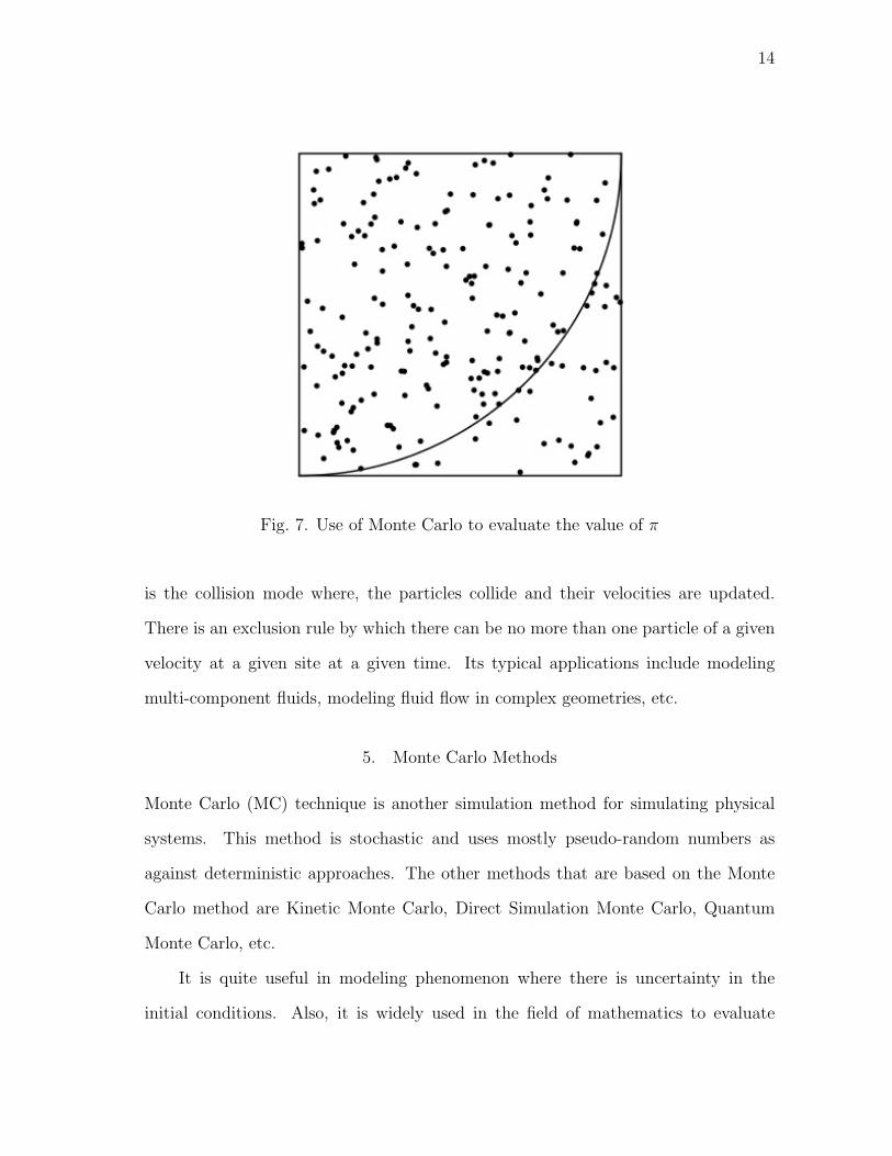
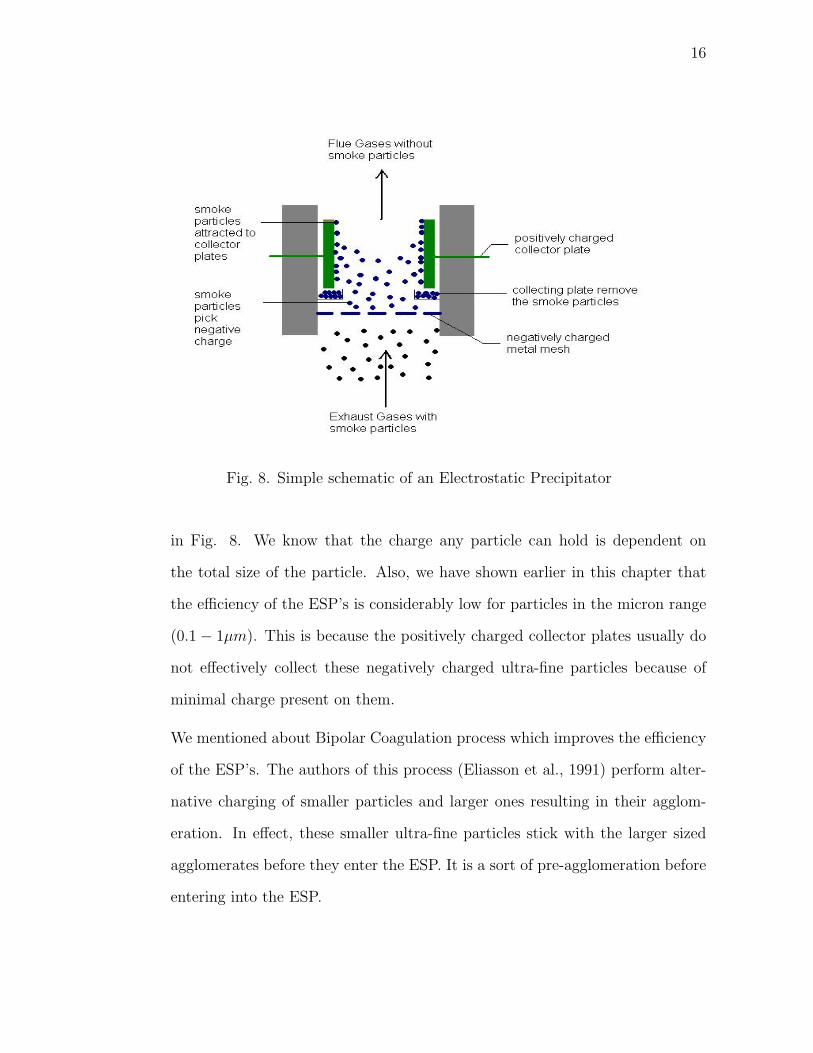
Electrostatic Precipitators (ESP). The working principle of an ESP is shown

16

Fig. 8. Simple schematic of an Electrostatic Precipitator

in Fig. 8. We know that the charge any particle can hold is dependent on

the total size of the particle. Also, we have shown earlier in this chapter that

the efficiency of the ESP’s is considerably low for particles in the micron range

(0.1− 1µm). This is because the positively charged collector plates usually do

not effectively collect these negatively charged ultra-fine particles because of

minimal charge present on them.

We mentioned about Bipolar Coagulation process which improves the efficiency

of the ESP’s. The authors of this process (Eliasson et al., 1991) perform alter-

native charging of smaller particles and larger ones resulting in their agglom-

eration. In effect, these smaller ultra-fine particles stick with the larger sized

agglomerates before they enter the ESP. It is a sort of pre-agglomeration before

entering into the ESP.

17

2. Powder Compaction

Simulations have been done on powder compaction using Discrete Element

method. In this model (Martina et al., 2003), the compaction occurs with

a plastic deformation at the particles’ contact area followed by a mutual re-

arrangement of particles. Their paper discusses features such as contact law,

relative density and the type of stress exerted on the particles and their effect

on the deformation mechanisms. They also showed how particle re-arrangement

plays an important role in powder compaction.

3. Synthesis of Titania Powders

A study on the particle agglomeration during the synthesis of titania powders

was done numerically based on colloidal stabilty using van der Waals attraction

and electrostatic repulsive forces (Kim et al., 1999). In this paper, they changed

the shape of the energy barrier as a result of increase of particle radius and this

allowed bigger particles to agglomerate more easily.

The chapters to follow will lay out the objectives and scope of this thesis. This

will be followed by a detailed description of Dissipative Particle Dynamics. Also, there

is a brief discussion on the procedure for the MATLAB and C-routine interface due

to our simulation requirements. We continue our discussion specifying the underlying

forces of attraction used as a part of the study and elaborate the algorithm used in

the work. Results and subsequent discussion on it follows this.

18

CHAPTER II

SCOPE AND OBJECTIVES

A. Scope

In the study of particle agglomeration, the various agglomeration mechanisms men-

tioned in the earlier chapter are important. Using different simulation techniques,

these mechanisms can be studied and applied. Simulations can be performed for dif-

ferent types of systems and many forms of the inter-particle forces can be modeled

accordingly.

We can use the simulation methods mentioned in Chap. I for our purpose if

performing experiments is determined to be involving. The choice of the simulation

method is based on the necessity of a deterministic or a probabilistic technique.

For the purpose of position and velocity updates for each particle, different types of

algorithms can be used. Algorithms such as Verlet, Velocity-Verlet, Euler, Leap-Frog,

Beeman aglorithm or DPD-VV schemes can be implemented depending on how much

accuracy is needed and how much it is suited to the method used.

Upon successful simulation of particle agglomeration, we can have a qualitative

understanding of the effect of the forces that cause agglomeration. Particles of dif-

ferent sizes and materials can be simulated to study the process of agglomeration.

Comparative results of the agglomerates that are formed as a result can be obtained.

B. Objectives

Our domain of work involves particles of size, 20nm and hence we select dissipative

particle dynamics due to its applicability in the mesoscale. Also because it is galilean

invariant and its hydrodynamic equations of mass and momentum being consistent

19

with the Navier-Stokes equations. We make use of a DPD-VV time integration scheme

in the context of DPD. A couple of inter-particle forces from the literature that cause

agglomeration are utilzied and upon successful simulation, we wish to characterize the

agglomerates and present a comparative study on the differences in the characteristics

of the agglomerate formed as a result.

The work in this thesis involves dynamic simulation. We do not use any com-

mercial particle simulation software and also wish to avoid post-processing the data

(particle positions and velocities) generated at each time-step as it involves a lot of

turnaround time. In this work, a novel methodology for dynamic simulation was

worked upon which involves interfacing the commercial software MATLAB and the

main computational C program. This is quite useful for small-particle simulations

where we can explore the effects of particular types of forces on the characteristics of

the agglomerates in a simple way.

20

CHAPTER III

DISSIPATIVE PARTICLE DYNAMICS: DESCRIPTION AND REQUIREMENTS

OF OUR PROBLEM

A. Theory

Dissipative Particle Dynamics, as mentioned earlier is a discrete particle simulation

methodolgy which accomodates larger length and time scales that is, it is very much

applicable in the mesoscale. Though initially introduced in 1992 by Hoogerbrugge

and Koelman, it lacked the much necessary theoretical framework. Three years later,

this was provided by Espanol when he proposed the statistical mechanics involved

with DPD (Espanol et al., 1998). His group formulated the stochastic differential

equations and the equivalent Fokker-Planck equation that correspond to the algo-

rithm of Hoogerbrugge and Koelman. Fokker-Planck equation governs the positions

and velocities of all the particles within the system. By doing so, he showed the

hydrodynamic behavior to be consistent with Navier-Stokes equations. Espanol and

Warren formulated the fluctuation-dissipation theorem for DPD which ensures the

proper thermodynamic equilibrium. Now, let us look at the features of DPD and its

constitutive equations.

B. Salient Features

DPD involves a set of particles, each of which moves in continuous space and discrete

time. Each set depicts the behavior of the group of molecules it contains. It involves

simulation of soft spheres, whose motion is governed by certain collision rules. The

following is the usual DPD we all know from the past work (Espanol et al., 1998).

The particles interact via three types of forces, a conservative force, FC , a random

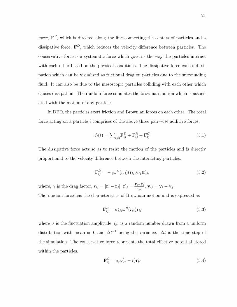
21

force, FR, which is directed along the line connecting the centers of particles and a

dissipative force, FD, which reduces the velocity difference between particles. The

conservative force is a systematic force which governs the way the particles interact

with each other based on the physical conditions. The dissipative force causes dissi-

pation which can be visualized as frictional drag on particles due to the surrounding

fluid. It can also be due to the mesoscopic particles colliding with each other which

causes dissipation. The random force simulates the brownian motion which is associ-

ated with the motion of any particle.

In DPD, the particles exert friction and Brownian forces on each other. The total

force acting on a particle i comprises of the above three pair-wise additive forces,

fi(t) =∑

j 6=iFD

ij + FRij + FC

ij (3.1)

The dissipative force acts so as to resist the motion of the particles and is directly

proportional to the velocity difference between the interacting particles.

FDij = −γωD(rij)(rij.vij)rij, (3.2)

where, γ is the drag factor, rij = |ri − rj|, rij = ri−rj

rij, vij = vi − vj

The random force has the characteristics of Brownian motion and is expressed as

FRij = σζijω

R(rij)rij (3.3)

where σ is the fluctuation amplitude, ζij is a random number drawn from a uniform

distribution with mean as 0 and ∆t−1 being the variance. ∆t is the time step of

the simulation. The conservative force represents the total effective potential stored

within the particles.

FCij = aij.(1− r)rij (3.4)

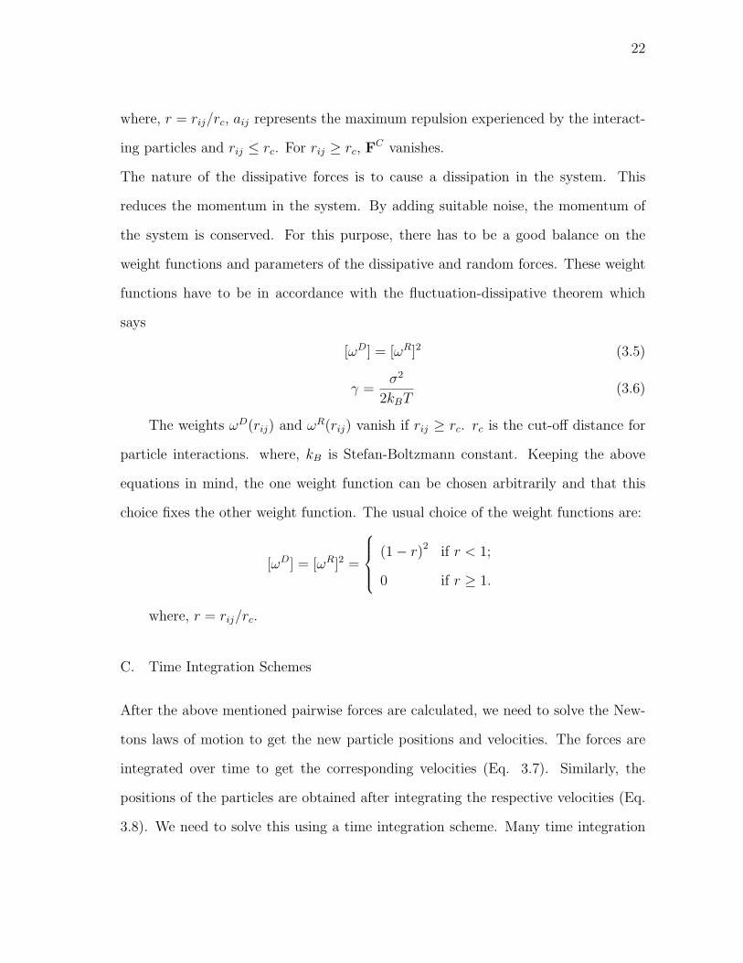
22

where, r = rij/rc, aij represents the maximum repulsion experienced by the interact-

ing particles and rij ≤ rc. For rij ≥ rc, FC vanishes.

The nature of the dissipative forces is to cause a dissipation in the system. This

reduces the momentum in the system. By adding suitable noise, the momentum of

the system is conserved. For this purpose, there has to be a good balance on the

weight functions and parameters of the dissipative and random forces. These weight

functions have to be in accordance with the fluctuation-dissipative theorem which

says

[ωD] = [ωR]2 (3.5)

γ =σ2

2kBT(3.6)

The weights ωD(rij) and ωR(rij) vanish if rij ≥ rc. rc is the cut-off distance for

particle interactions. where, kB is Stefan-Boltzmann constant. Keeping the above

equations in mind, the one weight function can be chosen arbitrarily and that this

choice fixes the other weight function. The usual choice of the weight functions are:

[ωD] = [ωR]2 =

(1− r)2 if r < 1;

0 if r ≥ 1.

where, r = rij/rc.

C. Time Integration Schemes

After the above mentioned pairwise forces are calculated, we need to solve the New-

tons laws of motion to get the new particle positions and velocities. The forces are

integrated over time to get the corresponding velocities (Eq. 3.7). Similarly, the

positions of the particles are obtained after integrating the respective velocities (Eq.

3.8). We need to solve this using a time integration scheme. Many time integration

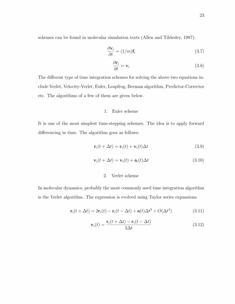
23

schemes can be found in molecular simulation texts (Allen and Tildesley, 1987).

∂vi

∂t= (1/m)fi (3.7)

∂ri

∂t= vi (3.8)

The different type of time integration schemes for solving the above two equations in-

clude Verlet, Velocity-Verlet, Euler, Leapfrog, Beeman algorithm, Predictor-Corrector

etc. The algorithms of a few of them are given below.

1. Euler scheme

It is one of the most simplest time-stepping schemes. The idea is to apply forward

differencing in time. The algorithm goes as follows:

ri(t + ∆t) = ri(t) + vi(t)∆t (3.9)

vi(t + ∆t) = vi(t) + ai(t)∆t (3.10)

2. Verlet scheme

In molecular dynamics, probably the most commonly used time integration algorithm

is the Verlet algorithm. The expression is evolved using Taylor series expansions.

ri(t + ∆t) = 2ri(t)− ri(t−∆t) + a(t)∆t2 + O(∆t4) (3.11)

vi(t) =ri(t + ∆t)− ri(t−∆t)

2∆t(3.12)

24

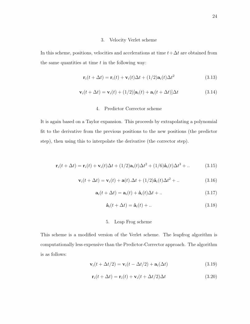
3. Velocity Verlet scheme

In this scheme, positions, velocities and accelerations at time t+∆t are obtained from

the same quantities at time t in the following way:

ri(t + ∆t) = ri(t) + vi(t)∆t + (1/2)ai(t)∆t2 (3.13)

vi(t + ∆t) = vi(t) + (1/2)[ai(t) + ai(t + ∆t)]∆t (3.14)

4. Predictor Corrector scheme

It is again based on a Taylor expansion. This proceeds by extrapolating a polynomial

fit to the derivative from the previous positions to the new positions (the predictor

step), then using this to interpolate the derivative (the corrector step).

ri(t + ∆t) = ri(t) + vi(t)∆t + (1/2)ai(t)∆t2 + (1/6)ai(t)∆t3 + .. (3.15)

vi(t + ∆t) = vi(t) + a(t).∆t + (1/2)ai(t)∆t2 + .. (3.16)

ai(t + ∆t) = ai(t) + ai(t)∆t + .. (3.17)

ai(t + ∆t) = ai(t) + .. (3.18)

5. Leap Frog scheme

This scheme is a modified version of the Verlet scheme. The leapfrog algorithm is

computationally less expensive than the Predictor-Corrector approach. The algorithm

is as follows:

vi(t + ∆t/2) = vi(t−∆t/2) + ai(∆t) (3.19)

ri(t + ∆t) = ri(t) + vi(t + ∆t/2)∆t (3.20)

25

6. Beeman algorithm

This algorithm is closely related to the Verlet algorithm

r(t + ∆t) = r(t) + v(t)∆t +2

3a(t)∆t2 − 1

6a(t−∆t)∆t2 + O(∆t4) (3.21)

This value is used to compute the accelerations at time t + ∆t, and these are used to

update the velocities using

v(t + ∆t) = v(t) +1

3a(t + ∆t)∆t +

5

6a(t)∆t− 1

6a(t−∆t)∆t + O(∆t3) (3.22)

7. Dissipative Particle Dynamics - Velocity Verlet algorithm

This algorithm was given out by Groot and Warren in 1997 (Groot, 1997). In the

context of DPD, they proposed this algorithm that has virtually no increase in com-

putation time. It goes as follows:

ri(t + ∆t) = ri(t) + ∆tvi(t) +1

2∆t2fi(t) (3.23)

vi(t + ∆t) = vi(t) + λ∆tfi(t) (3.24)

fi(t + ∆t) = fi(ri(t + ∆t), vi(t + ∆t)) (3.25)

vi(t + ∆t) = vi(t) +1

2∆t(fi(t) + fi(t + ∆t)) (3.26)

If the value of λ is taken as 1/2, we get back our velocity-verlet algorithm.

D. Boundary Conditions

Periodic boundary conditions are basically used to avoid the use of larger compu-

tational domains which requires greater computation time and effort. Instead, the

whole working domain can be broken down into several small sub-domains. Each

sub-domain is applied a periodic boundary condition on all the sides in common with

26

Fig. 9. Simple sketch of a periodic boundary condition

the adjacent sub-domains. Periodic boundary condition results in conservation of

mass, that is, as a few particles move out from one side of the cell, another particle

comes into the cell from the opposite side.

The periodicity can be employed on either sides of the sub-domain in a 1D case

(see fig. 9). It can be extended to six sides of the sub-domain volume for a 3D system.

Reflective boundary conditions are also employed to constrain the motion of the

particles within a specific region.

E. Past Work in DPD and Its Applications

After the formulation of the DPD theory many advances took place in this area. The

equilibrium and transport properties of the DPD fluid were explicitly calculated in

terms of the system parameters for the continuous time version of the DPD model

(Marsh et al., 1997). Their results gave out explicit predictions for the viscosities

and self-diffusion coefficient of the DPD fluid in terms of the model parameters:

density, friction, noise strength or equivalently temperature and range. Also, for the

equilibrium of a DPD simulation of a simple fluid, temperature was mentioned to

depend strongly on the time step. An analytic expression for this dependence was

27

developed and showed it to agree well with the simulation results (Marsh et al., 1997).

Until this point of time, only the mass and momentum conservation were achieved

and simulations were performed only under isothermal conditions, as energy could not

be conserved. A major breakthrough was done by incorporating internal energy into

the system, thereby allowing thermal analyses of systems. This novel technique was

brought forth separately by different authors (Avalos et al., 1997, Espanol 1997).

The mechanisms driving the change in internal energy of the particles are as-

sumed to be of two types. The first one is the work done by the dissipative forces

that increases the internal energy of the interacting particles. The work done is as-

sumed to be equally shared between the two interacting particles. The random force

on the other hand cools the particles transferring the internal energy back to me-

chanical energy. The interacting particles also can exchange internal energy among

themselves and hence there will be a mesoscopic heat flow. Along with this, we have

the random heat flow as well. The friction forces are due to the difference of mo-

mentum between the particles and the heat flow due to the temperature difference

between them. Finally, they arrive at the first fluctuation-dissipation theorem which

relates the random force with the temperature of the interacting particles and not

the thermodynamic temperature, T. This property enabled DPD to be applied to

problems other than an isothermal one. The fluctuation-dissipation theorem for heat

flux was also developed for the first time.(Avalos et al., 1997).

While the other theory (Espanol, 1997) said that the variation of the internal

energy is due to two different processes. One of these is the temperature differences

between the particles that producing changes in the internal energy through heat

conduction. The other is through the dissipation of energy due to the friction forces

and its transformation into internal energy by viscous heating. This theory also came

up with an internal energy and an entropy variable very much similar to the previous

28

theory. This showed that the viscous heating updating algorithm with a suitable

Verlet list conserves momentum to machine precision but energy conservation is only

in the limit of a vanishing time step.

By this time, people started to devise mechanisms to bring in the boundary con-

ditions into the simulations. A new way was brought out a way of treating the solid

boundaries (Revenga et al., 1998, Revenga et al., 1999). In one of these papers, they

talk about three different possible interactions of DPD particles with a solid boundary.

These three are Specular, Maxwellian and Bounce back reflections. In Specular reflec-

tions, the parallel component of the momentum of the particles is conserved and the

normal component reversed. The Maxwellian type has particles that are introduced

back into the system according to a Maxwellian distribution of velocities centered

at the velocity of the wall. Bounce back reflections have both the components of

velocities reversed. They came up with the results which showed the Bounce back

reflections producing stick/no slip boundary conditions for any value of the dimen-

sionless friction coefficient T . Bounce back depicts some anomalies is temperature

for lower T values. Specular reflections are free of any such problems regarding the

temperature. They conclude that for higher T values, all the wall reflecting laws pro-

duce stick boundary conditions. It is important to know this dimensionless friction

coefficient.

T =γλ

dVT

where γ is the friction coefficient, λ is the average distance between the particles, d is

the spatial dimension of the problem (d = 2 for a 2D problem) and VT =√

(kBT/m)

is the thermal velocity.

The late 90’s till the past year saw thermodynamic models being developed by

people. Applications of DPD began to show up thereafter. Simulations of oil/water

29

surfactant interfaces were performed to study surface forces and film rupture (Visser et

al., 2005). Simulations were performed on a gold nano-particle system and delineated

the factors that decide the success of their simulation (Juan et al., 2005). Simulations

of Poiseuille flow was used to measure the viscosity of the fluid (Backer et al., 2005).

Work has also been done on colloidal suspensions (Pryamitsyn et al., 2005), which

is a complex hydrodynamic phenomenon. Also, good amount of work was done on

lipid bi-layers in the past year (Jakobsen et al., 2005). A no-slip boundary condition

that can be used in DPD simulations was also brought out recently too (Pivkin et

al., 2005).

Over a period of time, DPD has been found to be a novel simulation technique.

As mentioned earlier in this chapter, it finds its applications ranging from the simple

study of flow around a cylinder to much complex simulation of a gold nano-particle

system (Juan et al., 2005). Agglomeration of red blood cells flowing in the capillary

channels was modeled in DPD by the authors (Dzwinel et al., 2002). A disadvantage

of DPD is the lack of a drag force between a central particle and the particle around

it. Their relative motion, as shown by the author (Espanol, 1998), might produce a

drag force provided many DPD particles are involved simultaneously. This reduces

the computational efficiency of this method. However, with the use of non-central

forces, the drag effect was captured using a smaller number of particles (Espanol,

1998).

Dissipative Particle Dynamics is a numerical technique that captures the advan-

tages of the continuum approach and atomistic simulation. From its various applica-

tions, we see that DPD has a lot of scope. It will particularly be useful in areas where

the continuum equations cannot easily be framed and where the use of atomistic

simulation will only use a vast amount of computational resources.

30

F. Requirements, Constraints and Approach of Simulation

For the purpose of simulation, we started out by a regular code written down in

C programming language. Initially, Lennard-Jones potential was used to gain an

understanding of particle interactions. The code worked and we post-processed the

data which is in the form of particle positions generated at each time-step. The first

particle simulation ensued and this was done in TECPLOT, a popular commercial

plotting software. We observed that there was a lot of turnaround time involved in

generating a single simulation. Our current process was to run the code for a series

of time-steps, read the output files of each time step into TECPLOT using a macro

and plotting the read particle positions of each time step.

We felt an instant need of developing a program run-and-plot technique. Our

restrictions were to avoid any possible use of particle simulation softwares such as

CERIUS2, CHARMM, AMBER, LAMMPS, etc. This is because if we want to run a

simulation for a small number of particles to observe effects of agglomeration, we do

not realistically need commercial simulation packages. Thus we explored the possibil-

ity of interfacing MATLAB and our C program. Next, we will introduce the feature

of MATLAB called MEX which we noticed not having used when it comes to particle

simulations. Most to all of the following have been cited from the MATLAB Manual.

1. MEX

MEX stands for MATLAB Executable. MATLAB is a high-productivity system

who’s specialty is eliminating time-consuming, low-level programming in compiled

languages like C or Fortran. But, on some occasions it is really advantageous to use

this feature of MEX. These occasions include the following:

1. Most of the codes which have been written a few years or even decades back

31

must have been written as a C or a Fortran program. With MEX, these codes

can be directly run from MATLAB instead of having to re-write as a M-file.

2. MATLAB codes which do not run fast enough due to inherent bottlenecks can

be optimized for speed by writing them effectively as a C/Fortran program.

Most of the versions of MATLAB are equipped with the MEX feature. All ver-

sions from MATLAB 6.5 (Release 13) have this feature. MEX-files are dynamically

linked routines or subroutines produced from a C or Fortran source code which, when

compiled, can be run from within MATLAB in the same way as MATLAB M-files.

Importantly, the external interface functions provide functionality to transfer data

between MEX-files and MATLAB. It also has an ability to call MATLAB functions

from C or Fortran code, that is, some features of MATLAB, if necessary, can be called

from the existing C or Fortran code.

MATLAB supports the use of a variety of compilers for building MEX-files.

When a mex file is compiled for the first time, MATLAB prompts you to allow it to

search for available compilers on that system. A default LCC compiler is installed

along with the MATLAB software. Based on its search for available compilers, we

get to select a compiler for our MEX-files. Since we were new to MEX, we selected

the default LCC compiler since it is easier to use and not any configuration after this

needs to be done.

2. Writing MEX-files

A MEX file has two main parts namely,

1. Computation routine

2. Gateway routine

32

The Computation routine is where all our necessary computation exists. If an

existing code is being used, then necessary changes have to be accommodated so that

it can used in MATLAB.

The Gateway routine is used to interface the Computation routine with MAT-

LAB by the use of mexFunction, which was discussed earlier on.

3. MEX and its application to our requirements

Our code mainly comprises of a main M-file and several supporting MEX files. The

M-file involves tasks such as running the entire simulation and dynamic plotting.

For the purpose of clarity, we subdivide our computations from a single MEX file

to many. In the M-file, we initialize all the variables such as particle positions,

velocities, etc., which are required to import/export into the MEX files. Once the

variables are initialized, we start compiling the MEX files sequentially as according

to our algorithm. More details on MEX have been mentioned in Appendix A.

4. Dynamic Simulation

As mentioned earlier, the main M-file also consists of the code for dynamic simulation.

To achieve dynamic simulation, we explored different types of techniques. But, the one

which suited our necessities was our plot-erase-plot methodology. This was achieved

with the EraseMode feature of MATLAB. This is one of the most commonly used

animation technique in MATLAB.

The MATLAB Manual says that the EraseMode property is appropriate for long

sequences of simple plots where the change from frame to frame is minimal. Its typical

usage is shown in Appendix B. Since, MATLAB environment will exist in many to all

research locations such as industries and universities, this approach can successfully

be used.

33

CHAPTER IV

APPROACH

A. Modified Features of DPD

We wanted to explore different types of inter-particle attractive forces from the litera-

ture. We eliminate the use of the repulsive force present in the form of the conservative

force because we require particles sticking to one another.

A few different types of attractive forces are the following. Along with their

description and the corresponding equation form, we present you the nature of these

forces graphically.

Firstly, we look at the basic van der Waals force of attraction from the literature

(Yu et al., 2003). As a part of their work, quantification of porosity and inter-particle

forces for equal sized spheres is done. We also know that van der Waals forces refer to

those forces which arise from the polarization of molecules into dipoles. Accordingly,

the van der Waals force when applied to two spheres that contain several atoms and

molecules can evaluated as follows

Fv =A

6

64R6(s + 2R)

(s2 + 4Rs)2(s2 + 4Rs + 4R2)2(4.1)

From the equation, A is the Hammaker constant which is based on material properties.

Its typical value is 10−20J. From the above relationship, we can see the characteristic

of this force.

It reduces to its alternate form, which is

Fv =a

s3(s2 − 1)2(4.2)

where, a is the maximum possible attraction and s is the inter-particle separation

34

Fig. 10. Plot of F/F0 vs. r/rc

35

and R is the particle radius.

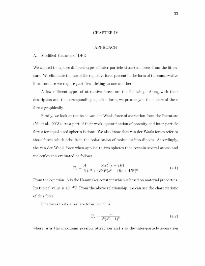
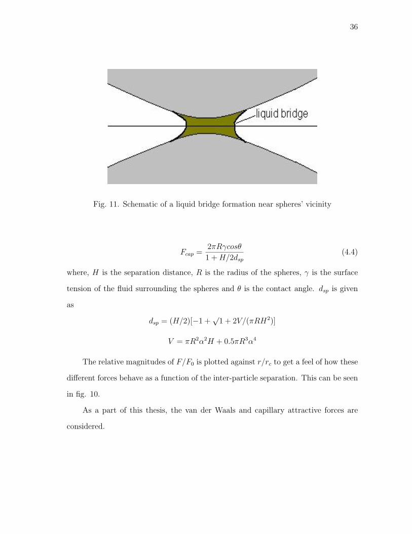
From the fig. 10, we see that the magnitude has a steep gradient very close

to the particles vicinity. It is considered a very weak force, not because it is less in

magnitude but because it is weak in its capability to exert substantial amount of force

at larger separations. Its strength lies in very close particle proximities.

Next, we wish to consider the electrostatic double-layer forces. A double layer

is a structure in ionized gas that consists of charge carriers (holes from valence band

and electrons from the conduction band). It consists of two parallel layers with op-

posite electrical charge. The sheets of charge cause a strong electric field and change

in electric potential across the double layer. The presence of a double layer requires

regions with a significant excess of positive or negative charge. From literature, (Isre-

alachvili, 1992) we get the expression for the electrostatic double-layer force between

two equal-sized spheres as,

Fe = 2πRσ2e−κD/κεε0 (4.3)

where, R is the radius of the spheres, σ is the surface charge density, κ is 1/Debye

length. Debye length is the distance beyond which any local electric field affects the

presence of free charge carriers between the double layer. D is the separation distance

between the two particles within the double layer, ε is the dielectric constant of the

medium and ε0 is the dielectric constant of vacuum.

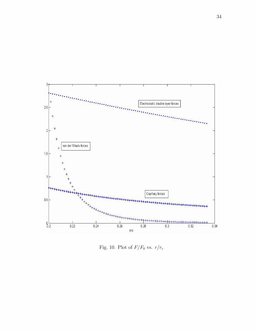
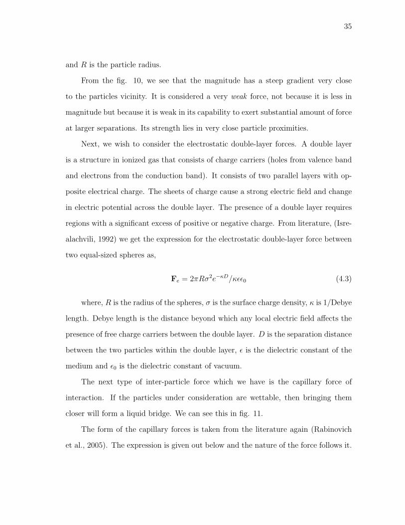
The next type of inter-particle force which we have is the capillary force of

interaction. If the particles under consideration are wettable, then bringing them

closer will form a liquid bridge. We can see this in fig. 11.

The form of the capillary forces is taken from the literature again (Rabinovich

et al., 2005). The expression is given out below and the nature of the force follows it.

36

Fig. 11. Schematic of a liquid bridge formation near spheres’ vicinity

Fcap =2πRγcosθ

1 + H/2dsp

(4.4)

where, H is the separation distance, R is the radius of the spheres, γ is the surface

tension of the fluid surrounding the spheres and θ is the contact angle. dsp is given

as

dsp = (H/2)[−1 +√

1 + 2V/(πRH2)]

V = πR2α2H + 0.5πR3α4

The relative magnitudes of F/F0 is plotted against r/rc to get a feel of how these

different forces behave as a function of the inter-particle separation. This can be seen

in fig. 10.

As a part of this thesis, the van der Waals and capillary attractive forces are

considered.

37

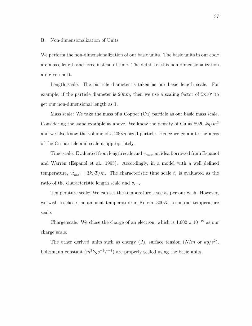
B. Non-dimensionalization of Units

We perform the non-dimensionalization of our basic units. The basic units in our code

are mass, length and force instead of time. The details of this non-dimensionalization

are given next.

Length scale: The particle diameter is taken as our basic length scale. For

example, if the particle diameter is 20nm, then we use a scaling factor of 5x107 to

get our non-dimensional length as 1.

Mass scale: We take the mass of a Copper (Cu) particle as our basic mass scale.

Considering the same example as above. We know the density of Cu as 8920 kg/m3

and we also know the volume of a 20nm sized particle. Hence we compute the mass

of the Cu particle and scale it appropriately.

Time scale: Evaluated from length scale and vrms, an idea borrowed from Espanol

and Warren (Espanol et al., 1995). Accordingly, in a model with a well defined

temperature, v2rms = 3kBT/m. The characteristic time scale tc is evaluated as the

ratio of the characteristic length scale and vrms.

Temperature scale: We can set the temperature scale as per our wish. However,

we wish to chose the ambient temperature in Kelvin, 300K, to be our temperature

scale.

Charge scale: We chose the charge of an electron, which is 1.602 x 10−19 as our

charge scale.

The other derived units such as energy (J), surface tension (N/m or kg/s2),

boltzmann constant (m2kgs−2T−1) are properly scaled using the basic units.

38

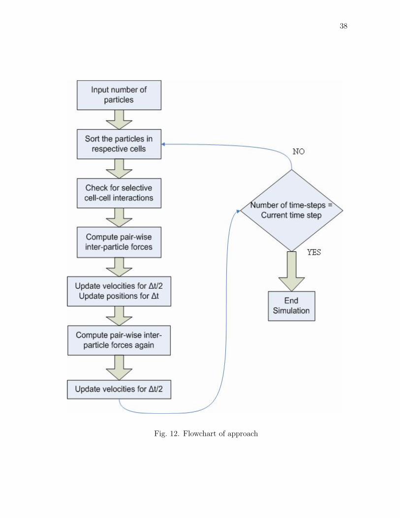
Fig. 12. Flowchart of approach

39

C. Algorithm

Our main computations are performed in a C program which is written in MEX

format. A detailed step-by-step algorithm of our code is given below.

1. We first initialize the particle positions randomly. The velocities are initialized

to follow a Gaussian distribution. The other essential parameters of the system

such as domain size, time step, number of time steps, cut-off radius are specified

2. Next, we compile all our mex files before starting the simulation.

3. The mex file associated with gridding the domain into cells is executed. The

whole domain is divided into A x A x A sized cells.

4. The main time loop begins

5. The mex file for the particles being assigned a cell number is executed. After

this, each particle is associated with its cell number.

6. The mex file for selective interactions is executed and all the pairwise inter-

particle forces are specified in this mex file. The forces are evaluated and re-

turned back to the Matlab workspace.

7. Next the mex file for updating the particle positions and velocities is executed.

8. The new particle positions and velocities are displayed on the screen

9. The main time loop ends

Our algorithm is depicted in the form of a flowchart. This can be seen in fig. 12.

40

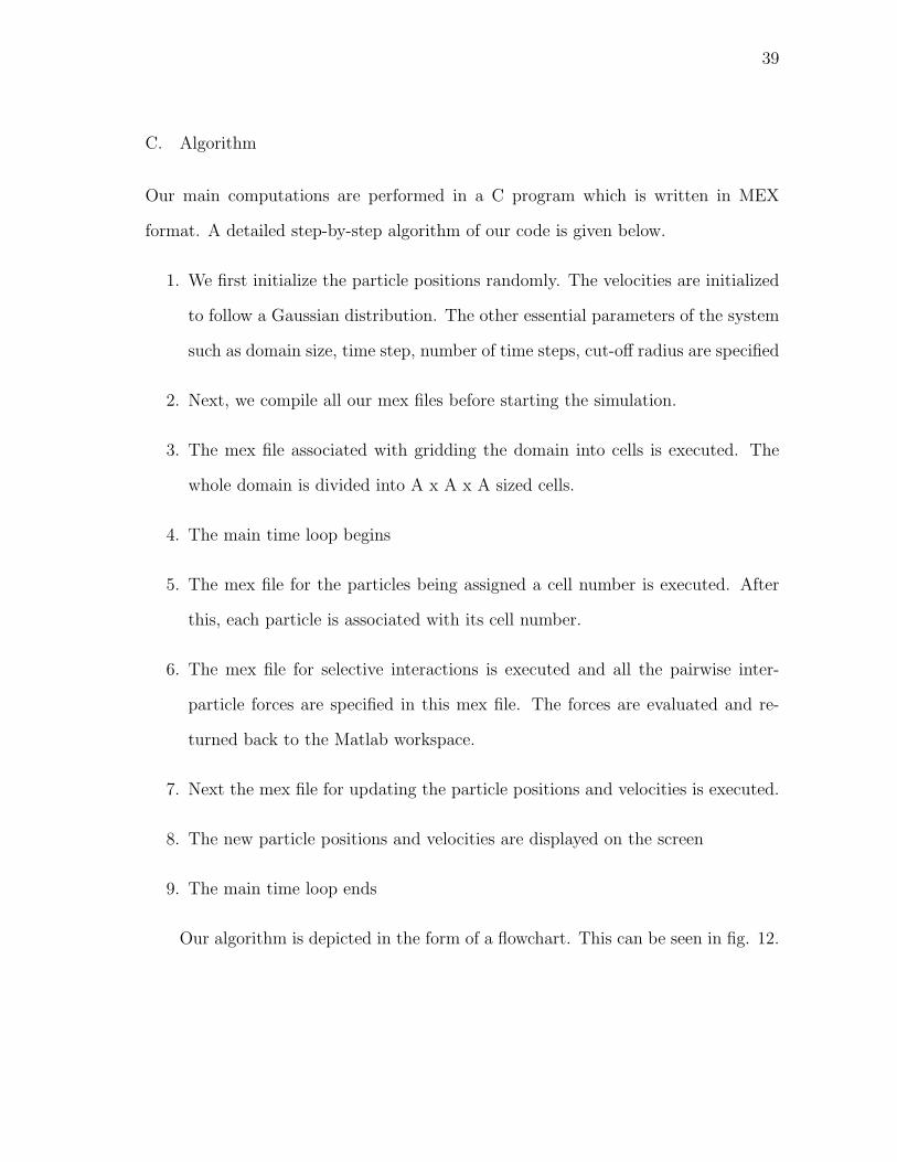
Fig. 13. Types of agglomerates

D. Characterizing Agglomerates

An agglomerate is said so if any two particles have their inter-particle distance less

than particle diameter. A tree agglomerate is one in which many agglomerates are

inter-connected to each other. Such tree agglomerates are fitted in a smallest fitting

ellipsoid. An ellipsoid is a higher dimensional analogue of the ellipse. The equation

of an ellipsoid is given as

x2

a2+

y2

b2+

z2

c2= 1

A typical prolate ellipsoid can be seen in fig. 14.

The characteristics of such agglomerates will be based on the following:

1. Number of particles present in any form of an agglomerates.

2. Number of single tree agglomerates or the ellipsoids enclosing them.

3. Classification of these ellipsoids.

41

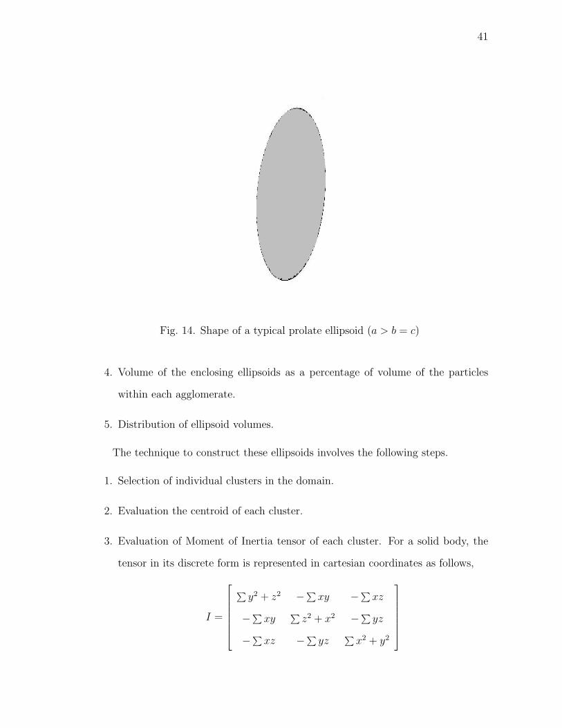
Fig. 14. Shape of a typical prolate ellipsoid (a > b = c)

4. Volume of the enclosing ellipsoids as a percentage of volume of the particles

within each agglomerate.

5. Distribution of ellipsoid volumes.

The technique to construct these ellipsoids involves the following steps.

1. Selection of individual clusters in the domain.

2. Evaluation the centroid of each cluster.

3. Evaluation of Moment of Inertia tensor of each cluster. For a solid body, the

tensor in its discrete form is represented in cartesian coordinates as follows,

I =

∑

y2 + z2 −∑xy −∑

xz

−∑xy

∑z2 + x2 −∑

yz

−∑xz −∑

yz∑

x2 + y2

42

x, y, z being the distances of every cluster from the centroid of the cluster.

4. The eigen values of this matrix gives the lengths of the semi-axes of the required

ellipsoids.

We need to remember that the moment of inertia of the cluster was calculated

using the distance of the centers of particles from the centroid of the cluster. To

consider an ellipsoid that captures not just these point particles but also the particles

with a diameter, we add 1 unit, that represents one particle diameter, to the lengths

of the semi-axes.

The next chapter will show the results that we achieved and a discussion of the

same.

43

CHAPTER V

RESULTS AND CONCLUSIONS

We present the results of agglomeration as a result of application of the forces men-

tioned in the previous chapter. The various parameters used in the computations

with the results and subsequent characterization of the agglomerates are also pre-

sented along with a relevant discussion and analysis.

A. Parameters in Computations

All the length units are non-dimensionalized to the particle diameter as mentioned

earlier. Our usual cut-off is 3 units or unless specified. The cut-off distance was

decided upon from a plot of the different forces of attraction beyond which we can

safely assume the respective forces to be negligible. This plot can be seen in Fig.

10. The plot shows the basic van der Waals, capillary and electrostatic double layer

forces of attraction and their dependence on the inter-particle separation.

The choice of σ was based on literature (Groot et al., 1999) where the selection

of the DPD parameters is done on the basis of a stable equilibrium temperature.

The time step δt is also selected using the ideas from this work (Groot et al., 1999).

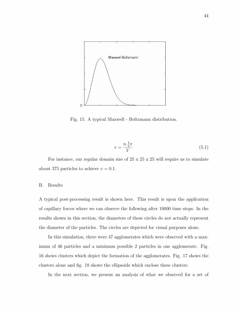
The velocities of the particles are initialized so as to follow the Maxwell-Boltzmann

distribution. A typical Maxwell-Boltzmann distribution can be seen in Fig. 15.

We attempt to achieve a volume density of around 0.1 and with this parameter

fixed, the domain size and number of particles is to be established. Keeping in mind

the particle diameter to be unity in our system of units, the volume density here is

defined by Eq. 5.1. V is the volume of our domain and n is the number of particles.

Volume density, v is

44

Fig. 15. A typical Maxwell - Boltzmann distribution.

v =n.4

3π

V(5.1)

For instance, our regular domain size of 25 x 25 x 25 will require us to simulate

about 375 particles to achieve v = 0.1.

B. Results

A typical post-processing result is shown here. This result is upon the application

of capillary forces where we can observe the following after 10000 time steps. In the

results shown in this section, the diameters of these circles do not actually represent

the diameter of the particles. The circles are depicted for visual purposes alone.

In this simulation, there were 47 agglomerates which were observed with a max-

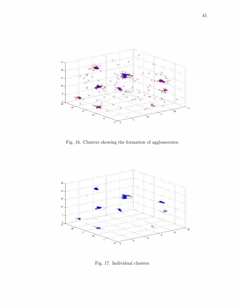
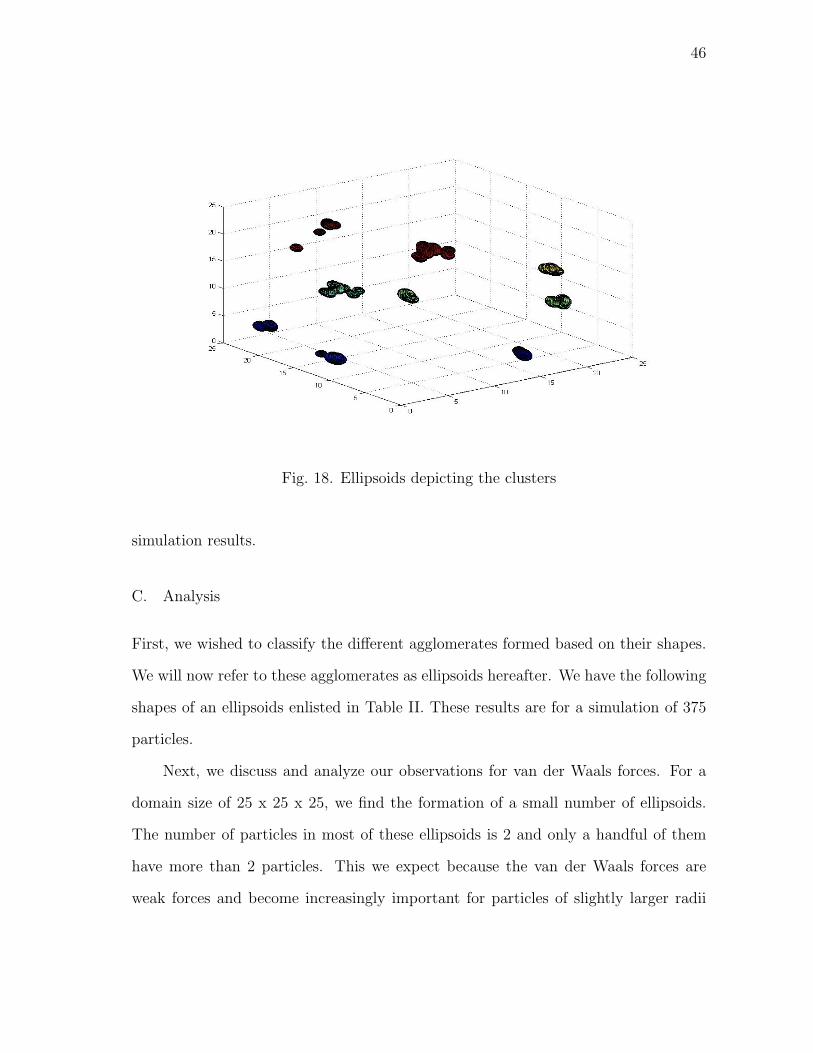
imum of 46 particles and a minimum possible 2 particles in one agglomerate. Fig.

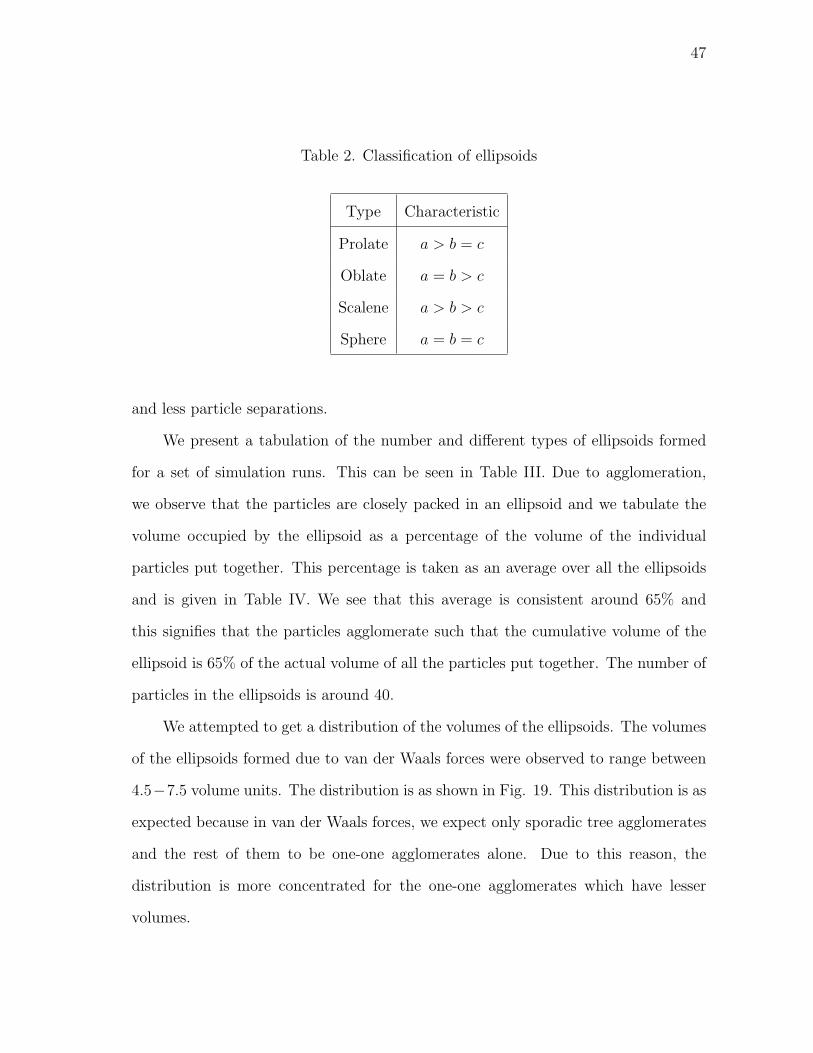
16 shows clusters which depict the formation of the agglomerates. Fig. 17 shows the

clusters alone and fig. 18 shows the ellipsoids which enclose these clusters.

In the next section, we present an analysis of what we observed for a set of

45

Fig. 16. Clusters showing the formation of agglomerates.

Fig. 17. Individual clusters.

46

Fig. 18. Ellipsoids depicting the clusters

simulation results.

C. Analysis

First, we wished to classify the different agglomerates formed based on their shapes.

We will now refer to these agglomerates as ellipsoids hereafter. We have the following

shapes of an ellipsoids enlisted in Table II. These results are for a simulation of 375

particles.

Next, we discuss and analyze our observations for van der Waals forces. For a

domain size of 25 x 25 x 25, we find the formation of a small number of ellipsoids.

The number of particles in most of these ellipsoids is 2 and only a handful of them

have more than 2 particles. This we expect because the van der Waals forces are

weak forces and become increasingly important for particles of slightly larger radii

47

Table 2. Classification of ellipsoids

Type Characteristic

Prolate a > b = c

Oblate a = b > c

Scalene a > b > c

Sphere a = b = c

and less particle separations.

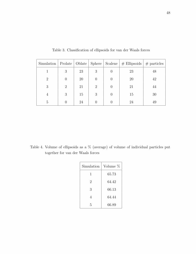
We present a tabulation of the number and different types of ellipsoids formed

for a set of simulation runs. This can be seen in Table III. Due to agglomeration,

we observe that the particles are closely packed in an ellipsoid and we tabulate the

volume occupied by the ellipsoid as a percentage of the volume of the individual

particles put together. This percentage is taken as an average over all the ellipsoids

and is given in Table IV. We see that this average is consistent around 65% and

this signifies that the particles agglomerate such that the cumulative volume of the

ellipsoid is 65% of the actual volume of all the particles put together. The number of

particles in the ellipsoids is around 40.

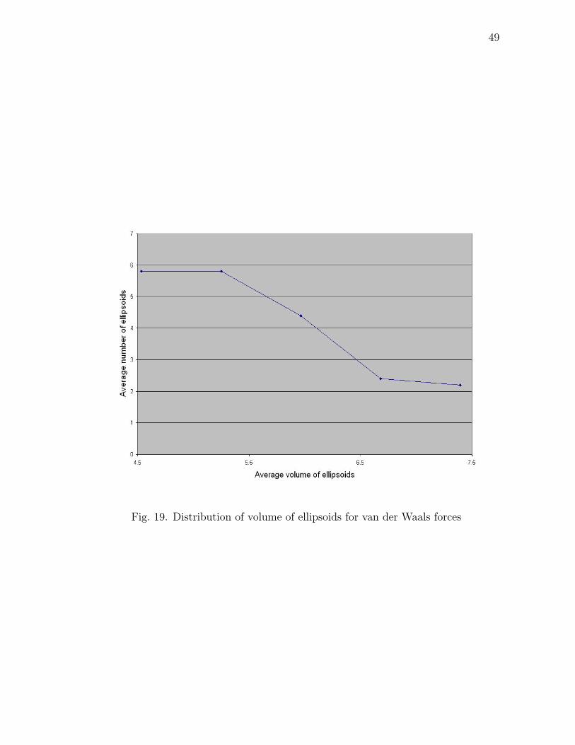
We attempted to get a distribution of the volumes of the ellipsoids. The volumes

of the ellipsoids formed due to van der Waals forces were observed to range between

4.5−7.5 volume units. The distribution is as shown in Fig. 19. This distribution is as

expected because in van der Waals forces, we expect only sporadic tree agglomerates

and the rest of them to be one-one agglomerates alone. Due to this reason, the

distribution is more concentrated for the one-one agglomerates which have lesser

volumes.

48

Table 3. Classification of ellipsoids for van der Waals forces

Simulation Prolate Oblate Sphere Scalene # Ellipsoids # particles

1 3 23 3 0 23 48

2 0 20 0 0 20 42

3 2 21 2 0 21 44

4 3 15 3 0 15 30

5 0 24 0 0 24 49

Table 4. Volume of ellipsoids as a % (average) of volume of individual particles put

together for van der Waals forces

Simulation Volume %

1 65.73

2 64.42

3 66.13

4 64.44

5 66.89

49

Fig. 19. Distribution of volume of ellipsoids for van der Waals forces

50

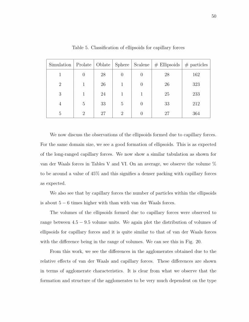
Table 5. Classification of ellipsoids for capillary forces

Simulation Prolate Oblate Sphere Scalene # Ellipsoids # particles

1 0 28 0 0 28 162

2 1 26 1 0 26 323

3 1 24 1 1 25 233

4 5 33 5 0 33 212

5 2 27 2 0 27 364

We now discuss the observations of the ellipsoids formed due to capillary forces.

For the same domain size, we see a good formation of ellipsoids. This is as expected

of the long-ranged capillary forces. We now show a similar tabulation as shown for

van der Waals forces in Tables V and VI. On an average, we observe the volume %

to be around a value of 45% and this signifies a denser packing with capillary forces

as expected.

We also see that by capillary forces the number of particles within the ellipsoids

is about 5− 6 times higher with than with van der Waals forces.

The volumes of the ellipsoids formed due to capillary forces were observed to

range between 4.5 − 9.5 volume units. We again plot the distribution of volumes of

ellipsoids for capillary forces and it is quite similar to that of van der Waals forces

with the difference being in the range of volumes. We can see this in Fig. 20.

From this work, we see the differences in the agglomerates obtained due to the

relative effects of van der Waals and capillary forces. These differences are shown

in terms of agglomerate characteristics. It is clear from what we observe that the

formation and structure of the agglomerates to be very much dependent on the type

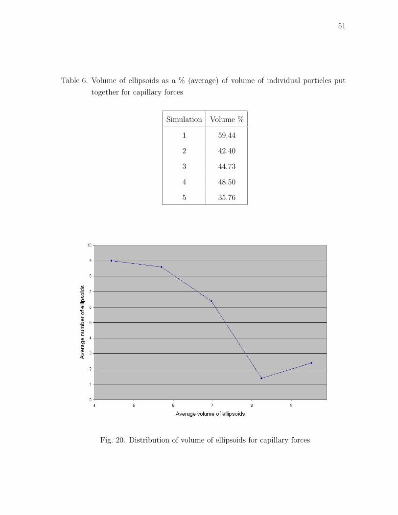
51

Table 6. Volume of ellipsoids as a % (average) of volume of individual particles put

together for capillary forces

Simulation Volume %

1 59.44

2 42.40

3 44.73

4 48.50

5 35.76

Fig. 20. Distribution of volume of ellipsoids for capillary forces

52

of force.

53

REFERENCES

[1] Alder B.J. and Wainwright T. E. (1959): Studies in molecular dynamics. I.

General method. - J. Chem. Phys., vol.31, pp.459-466.

[2] Allen M. P. and Tildesley D. J. (1987): Computer Simulation of Liquids, New

York: Oxford Press.

[3] Austin J. V. and Goldstein D. B. (1998): Simulation of supersonic rarefied at-

mospheric flows on Io. - 21st Intl. Symp. on Rarefied Gas Dynamics, Marseille,

France.

[4] Avalos J. B. and Mackie A. D. (1997): Dissipative particle dynamics with energy

conservation. - Europhys. Lett., vol.40, pp.141-146.

[5] Backer J. A., Lowe C. P., Hoefsloot H. C. J. and Iedema P. D. (2005): Poiseuille

flow to measure the viscosity of particle model fluids. - J. Chem. Phys., vol.122,

pp.154503.1-154503.6.

[6] Cagin T. (1993): Mechanical response of high performance polymers. - Materials

Theory and Modeling., vol.291, pp.321-324.

[7] Derjaguin B. V. and Landau L. (1941): Theory of the stability of strongly charged

lyphobic sols of the adhesion of strongly charged particles in solutions of elec-

trolytes. - Acta Physiochem. URSS, vol.14, pp.633-662.

[8] Dzwinel W., Yuen D. A. and Borycz K. (2002): Modeling of blood flow in cap-

illary vessels using discrete particles. - J. Mol. Model., vol.8, pp.33-43.

[9] Eliasson B. and Egli W. (1991): Bipolar coagulation - Modeling and applications.

- J. Aero. Sci., vol.22, pp.429-440.

54

[10] Espanol P. (1997): Dissipative particle dynamics with energy conservation. -

Europhys. Lett., vol.40, pp.631-636.

[11] Espanol, P. (1998): Fluid particle model. - Phys. Rev. E, vol.57, pp.2930-2948.

[12] Espanol P. and Warren P. (1995): Statistical mechanics of dissipative particle

dynamics. - Europhys. Lett., vol.30, pp.191-196.

[13] Frisch U., Hasslacher B. and Pomeau Y. (1986): Lattice gas automata for the

Navier-Stokes equations. - Phys. Rev. Lett., vol.56, pp.1505-1508.

[14] Fuchs N. A. (1964): The Mechanics of Aerosols, New York: Macmillan.

[15] Groot R. D. and Warren P. B. (1997): Dissipative particle dynamics: Bridging

the gap between atomistic and mesoscopic simulation. - J. Chem. Phys., vol.107,

pp.4423-4436.

[16] Hautanen J., Kilpelainen M., Kauppinen E.I., Jokiniemi J. and Lehtinen K.

(1995): Electrical agglomeration of aerosol particles in an alternating electric

field. - Aero. Sci. Tech., vol.22, pp.181-189.

[17] He X. and Luo L. (1997): Theory of the Lattice Boltzmann method: from the

Boltzmann equation to the Lattice Boltzmann equation. - Phys. Rev. E., vol.56,

pp.6811-6817.

[18] Hoogerbrugge P. J. and Koelman, J. M. V. A. (1992): Simulating microscopic

hydrodynamic phenomena with dissipative particle dynamics. - Europhys. Lett.,

vol.19, pp.155-160.

[19] Israelachvili J. N. (1992): Intermolecular and Surface Forces, San Diego: Aca-

demic Press .

55

[20] Jakobsen A. F. and Mouritsen O. G. (2005): Artifacts in dynamical simulations

of coarse-grained model lipid bilayers. - J. Chem. Phys., vol.122, pp.204901.1-

204901.11.

[21] Juan S.C.C, Hua C.Y., Chen C., Sun X. and Xi H. (2005): Dissipative particle

dynamics simulation of a gold nanoparticle system. - Mol. Sim., vol.31, pp.277-

282.

[22] Kart S. O., Tomak M., Uludogan M., and Cagin T. (2004): Liquid properties of

Pd-Ni alloys. - J. Noncryst. Sol., vol.337, pp.101-108.

[23] Kim J. C. and Auh K. H. (1999): Computer simulation on particle agglomeration

during the synthesis of titania powders. - Mod. Simul. Mater. Sci. Eng., vol.7,

pp.447-458.

[24] Lehtinen K., Jokiniemi J., Kauppinen E.I. and Hautanen J. (1995): Kinematic

coagulation of charged droplets in an alternating electric field. - Aero. Sci. Tech.,

vol.23, pp.422-430.

[25] Marsh C. A., Backx G. and Ernst M. H. (1997) Static and dynamic properties

of dissipative particle dynamics. - Europhys. Lett., vol.38, pp.411-415.

[26] Marsh C. A. and Yeomans J. M. (1997): Dissipative particle dynamics: the

equilibrium for finite time steps. - Europhys. Lett., vol.37, pp.511-516.

[27] Martina C.L., Bouvard D. and Shima S. (2003): Study of particle rearrangement

during powder compaction by the discrete element method. - J. Mech. Phys.

Solids, vol.51, pp.667-693.

[28] Parozzi F., Sandrelli G. and Masnaghetti A. (1988): Italian contribution to

TRAP-MELT code development. - IAEA International Symposium on Severe

56

Accidents in Nuclear Power Plants, Sorrento, Italy.

[29] Pivkin I. V. and Karniadakis G. E. (2005): A new method to impose no-slip

boundary conditions in dissipative particle dynamics. - J. Comp. Phys., vol.207,

pp.114-128

[30] Plimpton S. J. (1995): Fast parallel algorithms for short-range molecular dy-

namics. - J. Comp. Phys., vol.117, pp.1-19.

[31] Plimpton S. J. and Hendrickson B. A. (1995): Parallel molecular dynamics al-

gorithms for simulation of molecular systems. - (chapter in) Parallel Comput-

ing in Computational Chemistry, Amer. Chem. Soc., Symposium Series vol.592,

pp.114-132.

[32] Pope III C. A., Burnett R. T., Thun M. J., Calle E. E., Krewski D., Ito K. and

Thurston G. D. (2002): Lung cancer, cardiopulmonary mortality, and long-term

exposure to fine particulate air pollution. - J.A.M.A, vol.287, pp.1132-1141.

[33] Pryamitsyn V. and Ganesan V. (2005): A coarse-grained explicit solvent simula-

tion of rheology of colloidal suspensions. - J. Chem. Phys., vol.122, pp.104906.1-

104906.13.

[34] Rabinovich Y. I., Esayanur M. S. and Moudgil B. M. (2005): Capillary forces

between two spheres with a fixed volume liquid bridge: Theory and experiment.

- Langmuir 21, pp.10992-10997.

[35] Revenga M., Zuniga I. and Espanol P. (1999): Boundary conditions in dissipative

particle dynamics. - Comp. Phys. Comm., vol.121, pp.309-311.

[36] Revenga M., Zuniga I., Espanol P. and Pagonabarraga I. (1998): Boundary

models in DPD. - Int. J. Mod. Phys. C, vol.9, pp.1319-1328.

57

[37] Rothman D. and Zaleski S. (1994): Lattice-gas models of phase separation: inter-

faces, phase transitions and multiphase flow. - Rev. Mod. Phys., vol.66, pp.1417-

1480.

[38] Saffman P. G. and Turner J. S. (1956): On the collision of drops in turbulent

clouds. - J. Fluid Mech. vol.1, pp.16-30.

[39] Schmoluchowski M. (1917): Versuch einer mathematischen theorie der koagula-

tionskinetik kolloider lo sungen. - Z. Physik. Chem., vol.92, pp.129-154.

[40] Srinivasa A. R. and Phares D. J. (2004): Molecular dynamics with molecular

temperature. - J. Phys. Chem. A, vol.108, pp.6100-6108.

[41] Stillinger F. H. and Rahman, A. (1974): Improved simulation of liquid water by

molecular dynamics. - J. Chem. Phys., vol.60, pp.1545-1557.

[42] Verwey E. J. and Overbeek J. T. G. (1948): Theory of the Stability of Lyophobic

Colloids. - Amsterdam: Elsevier.

[43] Visser D.C., Hoefsloot H.C.J. and Iedema P.D. (2005): Modelling phase change

with DPD using a consistent boundary condition. - J. Comp. Phys., vol.205,

pp.626-639.

[44] Williams J. R., Hocking G. and Mustoe GGW (1985): The theoretical basis of

the discrete element method. - Proceedings of the NUMETA ’85 Conference,

pp.897-906, Swansea, U.K.

[45] Yu A.B., Feng C.L., Zou R.P. and Yang R.Y. (2003): On the relationship between

porosity and interparticle forces. - Powder Technology, vol.130, pp.70-76.

58

APPENDIX A

MEX: DETAILS

Necessary Components:

Coming to MEX-files, the following are the necessary components of a MEX-file:

1. #include mex.h (C/C++ MEX-files only)

2. mexFunction gateway in C/C++ (or SUBROUTINE MEXFUNCTION in Fortran)

3. The mxArray

4. API functions

Every C/C++ MEX file must have an #include mex.h statement.

The gateway routine to every MEX-file is called mexFunction. This is the entry

point MATLAB uses to access the DLL.

In C/C++, it is always -

mexFunction(int nlhs, mxArray *plhs[ ],

int nrhs, const mxArray *prhs[ ])

In Fortran, it is always -

SUBROUTINE MEXFUNCTION(NLHS, PLHS, NRHS, PRHS)

mxArray:

People with MATLAB understanding know that MATLAB is essentially built

around matrices and arrays. This holds good even for the use of external programs

within MATLAB. The mxArray is a special structure that contains MATLAB data.

It is the C representation of a MATLAB array. All types of MATLAB arrays (scalars,

vectors, matrices, strings, cell arrays, etc.) are mxArrays. The mxArray declaration

59

corresponds to the internal data structure that MATLAB uses to represent arrays.

Some of the information contained within the mxArray structure is:

• The MATLAB variable’s name

• Dimensions

• Data Type

• Whether Real or Complex

Its typical representation would be of the form -

mxArray *array;

API - mx and mex routines:

These are a set of MATLAB Application Program Interface (API) subroutines

to perform the tasks required for running an external program from MATLAB. These

are used after the array declaration as mentioned above.

mx* functions are used to access data inside the mxArrays. They are also used

to do memory management and to create and destroy mxArrays. The tasks which

can be achieved using mx* functions are creating arrays, accessing arrays, modifying

arrays and memory management. Managing memory is best used through these API

subroutines than use the ones used in C programming.

The mex* functions perform tasks back in MATLAB. Useful tasks include entry

point to C MEX-files, issue error message and return to MATLAB, execute MAT-

LAB command in caller’s workspace, call MATLAB function or user-defined M-file

or MEX-file, get copy of variable from the workspace, ANSI C printf style output

routine and issue warning messages.

Compiling the MEX file:

60

Once the MEX file has been written using the above mentioned directions, save

it with the appropriate extension. For example, if the MEX file was written in C,

save the file as filename.c. For files written in Fortran, files are to be saved as

filename.f. Once this is accomplished, the next step is to compile it.

For compiling purposes, type mex followed by the filename with its appropriate

extension in the MATLAB command prompt. The following shows an example.

>> mex filename.c

>> mex filename.f

If the code has no errors, the code has successfully been compiled into its equiv-

alent .dll extension. DLL stands for Dynamically Linked Library.

Simulation with MEX:

The main tasks that we need to perform for achieving a running simulation are:

1. After successfully compiling a MEX file, we need to run it just like any other

code. For this, we need to type the name of the mex file without its file extension

in the MATLAB command prompt. For example, if filename.c is compiled,

then type filename in the command prompt.

2. To import/export the MATLAB variables from the workspace to the MEX

file, we need to use API functions. The following will illustrate its usage:

mxArray *array_ptr;

double *element_ptr;

array_ptr = mexGetVariable(’’base’’, ’’workspacevariable’’);

element_ptr = mxGetPr(array_ptr);

...

Perform necessary computations

61

...

mexPutVariable(’’base’’,’’workspacevariable’’,array_ptr);

// One can use a new variable name while exporting into the workspace

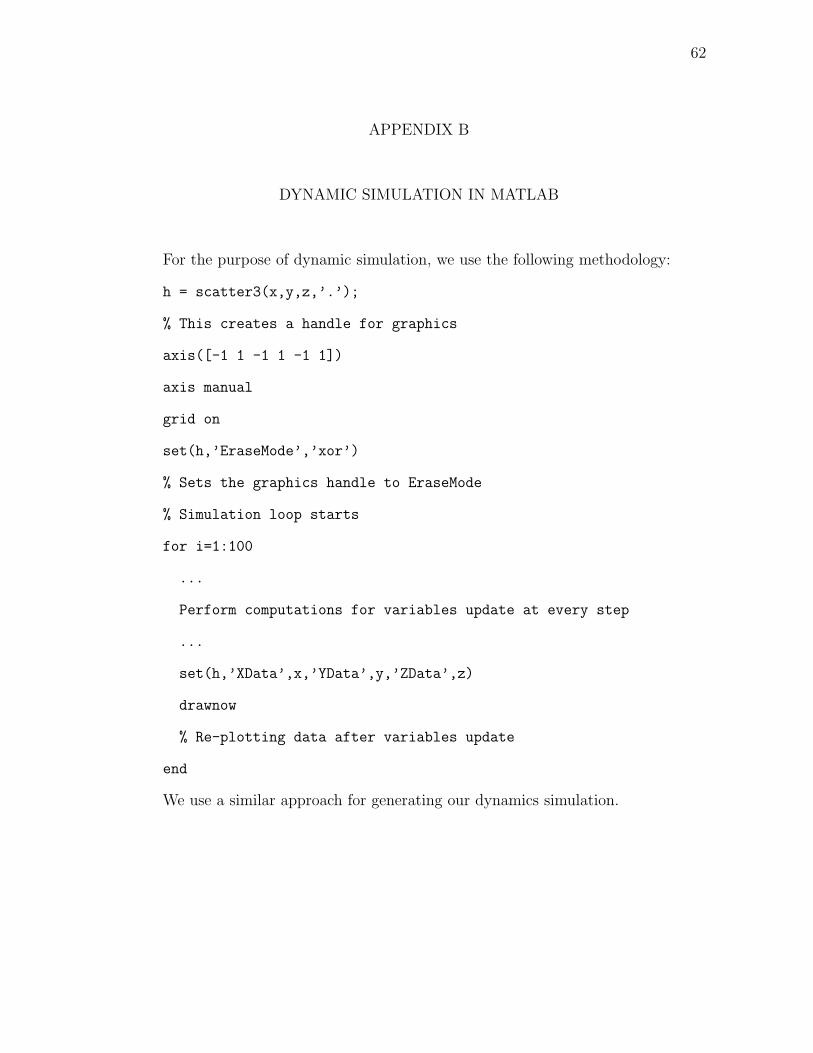
62

APPENDIX B

DYNAMIC SIMULATION IN MATLAB

For the purpose of dynamic simulation, we use the following methodology:

h = scatter3(x,y,z,’.’);

% This creates a handle for graphics

axis([-1 1 -1 1 -1 1])

axis manual

grid on

set(h,’EraseMode’,’xor’)

% Sets the graphics handle to EraseMode

% Simulation loop starts

for i=1:100

...

Perform computations for variables update at every step

...

set(h,’XData’,x,’YData’,y,’ZData’,z)

drawnow

% Re-plotting data after variables update

end

We use a similar approach for generating our dynamics simulation.

63

VITA

Srinivas Praveen Mokkapati was born in Chennai, India. He was primarily

brought up in Hyderabad, India where he did most of his schooling. He received

his Bachelor of Engineering degree in Mechanical Engineering from Osmania Univer-

sity, Hyderabad in 2004. Thereafter, he joined the Department of Mechanical En-

gineering at Texas A&M University in Fall 2004. He received his Master of Science

degree in Mechanical Engineering in December 2006. He can be reached through

his thesis advisor, Dr. Arun R. Srinivasa, Department of Mechanical Engineering,

Texas A&M University, College Station, TX 77840-3123. He can also be reached on

mspraveen@gmail.com.