Simulation of multiphase flow in hydrocyclone

P. Rudolf 1 1Brno University of Technology, Faculty of Mechanical Engineering, Technická 2896/2, Brno 61669, Czech Republic

Abstract. Multiphase gas-liquid-solid swirling flow within hydrocyclone is simulated. Geometry and boundary conditions are based on Hsieh’s 75 mm hydrocyclone. Extensive simulations point that standard mixture model with careful selection of interphase drag law is suitable for correct prediction of particle classification in case of dilute suspensions. However this approach fails for higher mass loading. It is also confirmed that Reynolds stress model is the best choice for multiphase modeling of the swirling flow on relatively coarse grids.

1 Introduction Hydrocyclones are widely used in processing

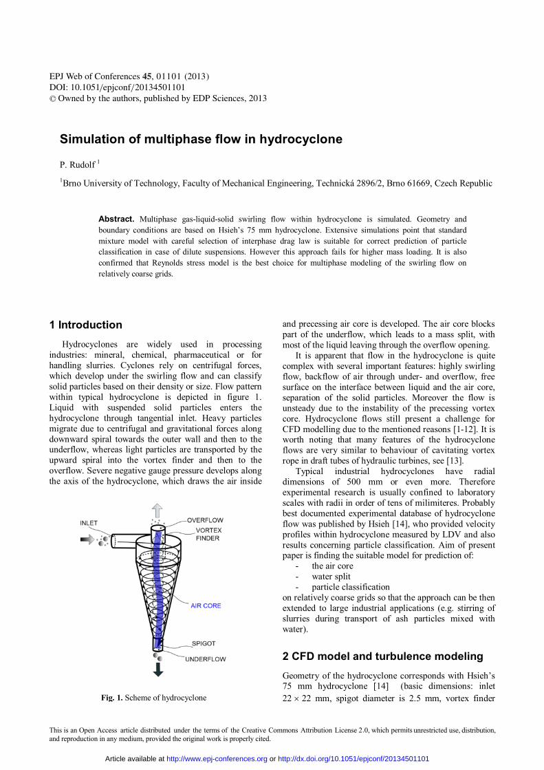
industries: mineral, chemical, pharmaceutical or for handling slurries. Cyclones rely on centrifugal forces, which develop under the swirling flow and can classify solid particles based on their density or size. Flow pattern within typical hydrocyclone is depicted in figure 1. Liquid with suspended solid particles enters the hydrocyclone through tangential inlet. Heavy particles migrate due to centrifugal and gravitational forces along downward spiral towards the outer wall and then to the underflow, whereas light particles are transported by the upward spiral into the vortex finder and then to the overflow. Severe negative gauge pressure develops along the axis of the hydrocyclone, which draws the air inside

and precessing air core is developed. The air core blocks part of the underflow, which leads to a mass split, with most of the liquid leaving through the overflow opening.

It is apparent that flow in the hydrocyclone is quite complex with several important features: highly swirling flow, backflow of air through under- and overflow, free surface on the interface between liquid and the air core, separation of the solid particles. Moreover the flow is unsteady due to the instability of the precessing vortex core. Hydrocyclone flows still present a challenge for CFD modelling due to the mentioned reasons [1-12]. It is worth noting that many features of the hydrocyclone flows are very similar to behaviour of cavitating vortex rope in draft tubes of hydraulic turbines, see [13].

Typical industrial hydrocyclones have radial dimensions of 500 mm or even more. Therefore experimental research is usually confined to laboratory scales with radii in order of tens of milimiteres. Probably best documented experimental database of hydrocyclone flow was published by Hsieh [14], who provided velocity profiles within hydrocyclone measured by LDV and also results concerning particle classification. Aim of present paper is finding the suitable model for prediction of:

- the air core - water split - particle classification

on relatively coarse grids so that the approach can be then extended to large industrial applications (e.g. stirring of slurries during transport of ash particles mixed with water).

2 CFD model and turbulence modeling Geometry of the hydrocyclone corresponds with Hsieh’s 75 mm hydrocyclone [14] (basic dimensions: inlet 22 22 mm, spigot diameter is 2.5 mm, vortex finder

Fig. 1. Scheme of hydrocyclone

This is an Open Access article distributed under the terms of the Creative Commons Attribution License 2 0 , which . permits unrestricted use, distributiand reproduction in any medium, provided the original work is properly cited.

on,

EPJ Web of ConferencesDOI: 10.1051/C© Owned by the authors, published by EDP Sciences, 2013

,epjconf 201/

01101 (2013)4534501101

Article available at http://www.epj-conferences.org or http://dx.doi.org/10.1051/epjconf/20134501101

EPJ Web of Conferences

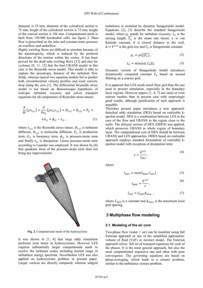
diameter is 25 mm, diameter of the cylindrical section is 75 mm, height of the cylindrical section is 75 mm, height of the conical section is 186 mm. Computational mesh is built from 150 000 hexahedral cells, see figure 2. Mass flow is prescribed on the inlet and constant static pressure on overflow and underflow. Highly swirling flows are difficult to simulate because of the anisotropicity, which is induced by the prefered directions of the motion within the vortex. It has been proved for the draft tube swirling flows [13] and also for cyclones [8, 11, 12] that the best URANS model in this case is the Reynolds stress model. This model is able to capture the anisotropic features of the turbulent flow fields, whereas typical two equation models fail to predict both circumferential velocity profiles and axial velocity drop along the axis [1]. The differential Reynolds stress model is not based on Boussinesque hypothesis of isotropic turbulent viscosity and solves transport equations for all components of Reynolds stress tensor:

휕휕푡 휌휏 , +

휕휕푥 휌푣 휏 , = 퐷 , +퐷 , + 푃 +

+퐺 +휙 − 휀 , (1) where 휏 , is the Reynolds stress tensor, 퐷 , is turbulent diffusion, 퐷 , is molecular diffusion, 푃 is production term, 퐺 is buoyancy term, 휙 is pressure-strain term and finally 휀 is dissipation. Linear pressure-strain term according to Launder was employed. It was shown by [4] that quadratic form of the pressure-strain term does not bring any improvements.

It was shown in [1, 4] that large eddy simulation performs even better in hydrocyclones. However LES requires substantially larger computational mesh to resolve the turbulent scales including inertial range of turbulence energy spectrum. Nevertheless LES was also applied on hydrocyclone problem in present paper. Larger vortices are directly computed, whereas subgrid

turbulence is modeled by dynamic Smagorinski model. Equations (2), (3) describe the standard Smagorinski model, where 휇 stands for turbulent viscosity, 퐿 is the mixing length, 푆 is the strain rate tensor, 휅 is von Kármán constant, 푑 is closest distance to the wall, Δ = 푉 / is the grid size and 퐶 is Smagorinski constant.

휇 = 휌퐿 푆 , (2)

퐿 = 푚푖푛(휅푑, 퐶 Δ), (3)

Dynamic version of Smagorinski model introduces dynamically computed constant C based on second filtering on a coarser grid.

It is apparent that LES needs much finer grid than the one used in present simulation, especially in the boundary layer regions. However papers [1, 4, 7] use same or even coarser meshes than in present case with surprisingly good results, although justification of such approach is arguable. Therefore present paper introduces a new approach: detached eddy simulation (DES) based on realizable k-epsilon model. DES is a combination between LES in the core of the flow and URANS in the region close to the walls. The delayed version of DES (DDES) was applied, which preserves URANS in whole region of boundary layer. The computational cost of DES should be between URANS and LES approaches. DDES based on realizable approach employs standard formulation of realizable k-epsilon model with exception of dissipation term:

휀 =푘 /

푙 , (4)

where

푙 = 푚푖푛(푙 , 푙 ), (5)

푙 =푘 /

휀 , (6)

푙 = 퐶 훥 , (7)

where 퐶 is a constant and Δ is the maximum local grid spacing.

.3 Multiphase flow modeling

3.1. Modeling of the air core

Two-phase flow (water + air) can be modeled using full Eulerian approach or one of the simplified approaches: volume of fluid (VoF) or mixture model. The Eulerian approach solves full set of transport equations for each of the phases. It is the most general approach, but also the most computational expensive one and often with poor convergence. The governing equations are based on phase-averaging, which leads to a closure problem, similar to the turbulence closure problem.

Fig. 2. Computational mesh of the hydrocyclone

01101-p.2

EFM 2012

General phased averaged variable 휙:

휙 =훼 휙훼 ,

(8)

where 훼 is the volume fraction of the phase k. Closing of the system rests on empirical formulas for interphase exchange of momentum.

3.1.1 Volume of fluid (VoF)

VoF is used to model flow of two or more immiscible fluids. VoF tracks location of the interface using a special form of continuity equation:

휕훼휕푡 + 훼

휕푣휕푥 = 0,

(9)

where 훼 is the volume fraction of the second phase. Volume fraction transport equation is solved implicitly and modified HRIC scheme is used for interpolation of the face fluxes. Unsteady computations are carried out with time step ∆푡 = 0.0005 s for RSM simulations and ∆푡 = 0.00001s for DDES and LES simulations. Advection term in momentum equation is interpolated with QUICK scheme, in turbulence equations with second order upwind scheme. Pressure on the cell faces is interpolated via PRESTO scheme. Operating point of the hydrocyclone is given by mass flow rate 1.117 kg.s-1.

3.1.2 Mixture model

Mixture model is a simplification of the full Eulerian model by making two main assumptions:

1. The dispersed phase flows with slip velocity relative to the continuous phase.

2. The interphase momentum exchange is via simple empirical drag formula.

It means that the momentum equation is only solved for the mixture, where mixture properties are defined as follows:

푣 , =∑ 훼 휌 푣

휌 , (10)

휌 = 훼 휌 , (11)

휇 = 훼 휇 , (12)

The volume fraction transport equation is then: 휕휕푡(훼 휌 )+

휕(훼 휌 푣 , )휕푥 = −

휕휕푥 훼 휌 푣 , ,

(13)

Where the drift velocity 푣 , is obtained from following expression:

푣 , = 푣 , −훼 휌 푣 ,

휌 , (14)

where 푣 , is velocity of the k-th phase relative to the primary phase (water). This velocity is calculated from so called algebraic slip mixture model (ASM). It is apparent that by neglecting the drift velocity volume of fluid model (VoF) is recovered. Basic ingredient of ASM is expression for drag between the continuous and dispersed phases. QUICK interpolation scheme is used for flux interpolation in the volume fraction equation. Interpolation of other terms and time step of the unsteady computation is the same as in the case of VoF simulation. Only RSM model is employed in combination with mixture model.

3.2 Modeling of particle classification

3.1.2 Lagrangian tracking

Let us assume a three-phase system: flow of water, air and dispersed solid particles. The Lagrangian approach is based on integration of the particle paths throughout the computational domain. Interactions with the continuous phase and among the particles can be made by one-, two- or four-way coupling. Flow of the continuous phase is predicted either using VoF or mixture model. Tracking is realized by writing force equilibrium equation of a solid particle assuming different types of forces according to complexity of the model. This approach is only suitable when reasonable number of particles is tracked and when the suspension is rather dilute (max 5-10% mass fraction of the solid phase).

3.1.2 Eulerian prediction of the phase concentration

Eulerian approach is based on assuming that the solid phase can be treated as continuum. Either the full Eulerian approach with employing momentum transport equations for each phase or simplified mixture approach can be applied. Present paper focuses on latter one, because of the reduced computational effort and better convergence properties. Mixture model uses the same theory as described above plus an enhancement for granular flows. The enhancements are based on the analogy between particulate flows and gas flow. Concept of granular temperature and interparticle collisions is introduced. Model is closed by several empirical formulas, namely for calculation of granular temperature, granular viscosity, distribution function, which characterizes the particle collisions and solids pressure. Further, drag formula has to be prescribed for the interphase momentum exchange between the primary phase and solid particles. The maximum packing limit of the particles in the present simulation is assumed to be

01101-p.3

EPJ Web of Conferences

0.6, which corresponds to random close packing. It is obvious that this model has many “free” parameters that have to be tuned for the particular type of the granular flow. Advantage of this approach over the Lagrangian tracking is application to flows with higher loading of the solid phase. However previous papers lack the information on choice of the free parameters and sensitivity of the results to this choice. It is one of the aims of the present paper to finetune the model parameters for the particle separation in the hydrocyclone. Table 1 summarizes the earlier contributions to hydrocyclone flow modeling using the experiment of Hsieh [14].

Table 1. Review of the previous hydrocyclone modelling approaches based on experiment of Hsieh [14]

4 Results

The results are organized into two independent sets of simulations:

1. Two-phase flow simulations to assess velocity profiles, air core diameter and water split ratio using VoF and mixture models for multiphase modelling and RSM, DDES and LES models for turbulence description.

2. Three-phase flow simulations using mixture model and RSM to assess particle classification for two different mass loadings.

All experimental data are based on [14].

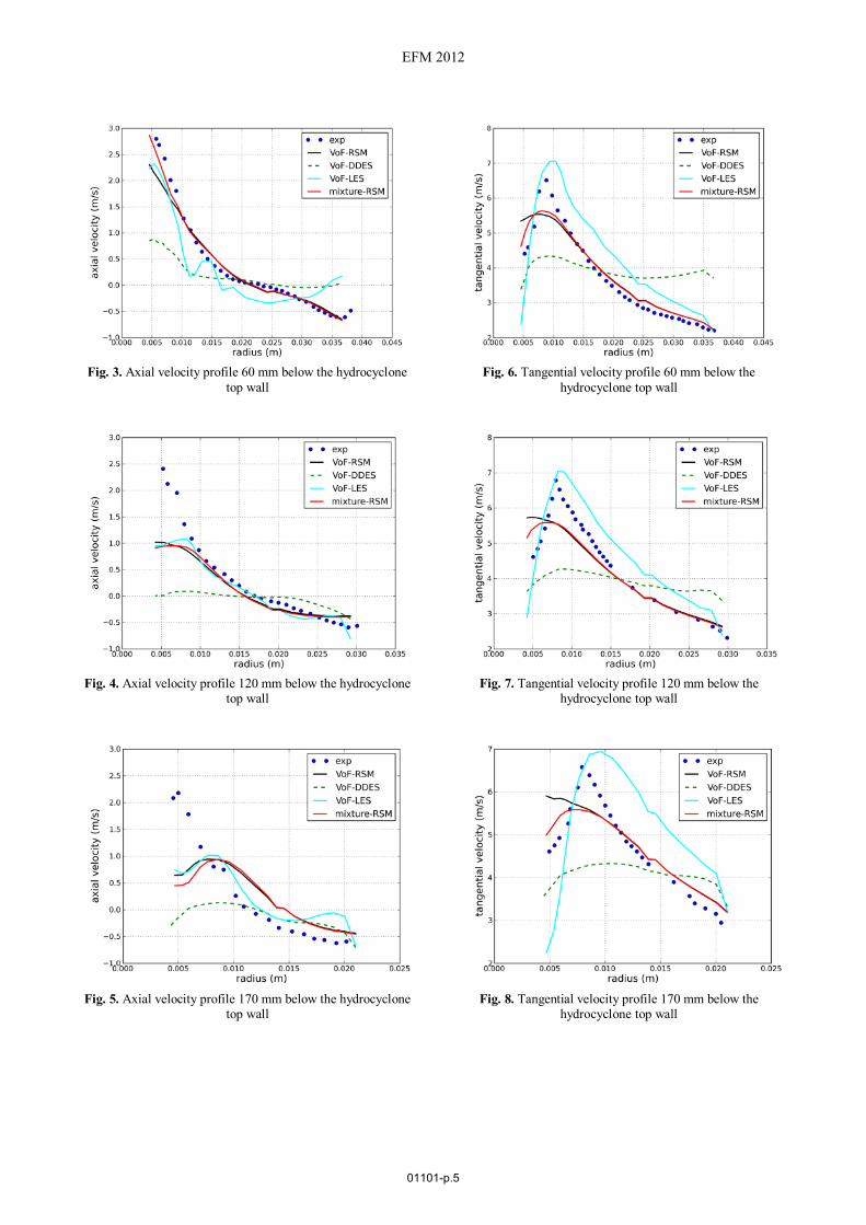
4.1 Velocity profiles

Axial and tangential velocity components were evaluated in 3 stations corresponding with measuring sections of Hsieh [14]. Figures 3-8 summarize comparison of the data from simulation against LDV measurements. The first striking feature is big discrepancy between measurement and DDES simulation. DDES is not able to capture the rise of tangential velocity towards hydrocyclone axis and then decline, which is characteristic for Lamb type vortex. It means it is not able to predict the correct rate of swirling. This result is surprising, because the simulation level of DDES should be able to depict quite accurately the large scale turbulent motion.

On the other hand, LES overpredicts the magnitude of tangential velocities in the potential part of the vortex. LES also provides incorrect description of the axial velocity profile in the near wall region, see figures 3 and 5. It has to be stressed however that the mesh is relatively coarse and near wall resolution of the mesh leads to y+ values in range 70-90, which is unacceptable for reliable LES simulation. This result is in contradiction with papers [1, 7], where meshes of similar size or even coarser were applied with much more realistic results.

Reynolds stress model provided the best results of all applied approaches. RSM is capable to provide very accurate description of the velocity profiles in the potential (outer) part of the vortex. Peak of the profile is underestimated and shifted toward the hydrocyclone axis. This shift is more pronounced on sections 120 and 170 mm from top wall and leads to discrepancy in prediction of the axial velocity profile near the air core.

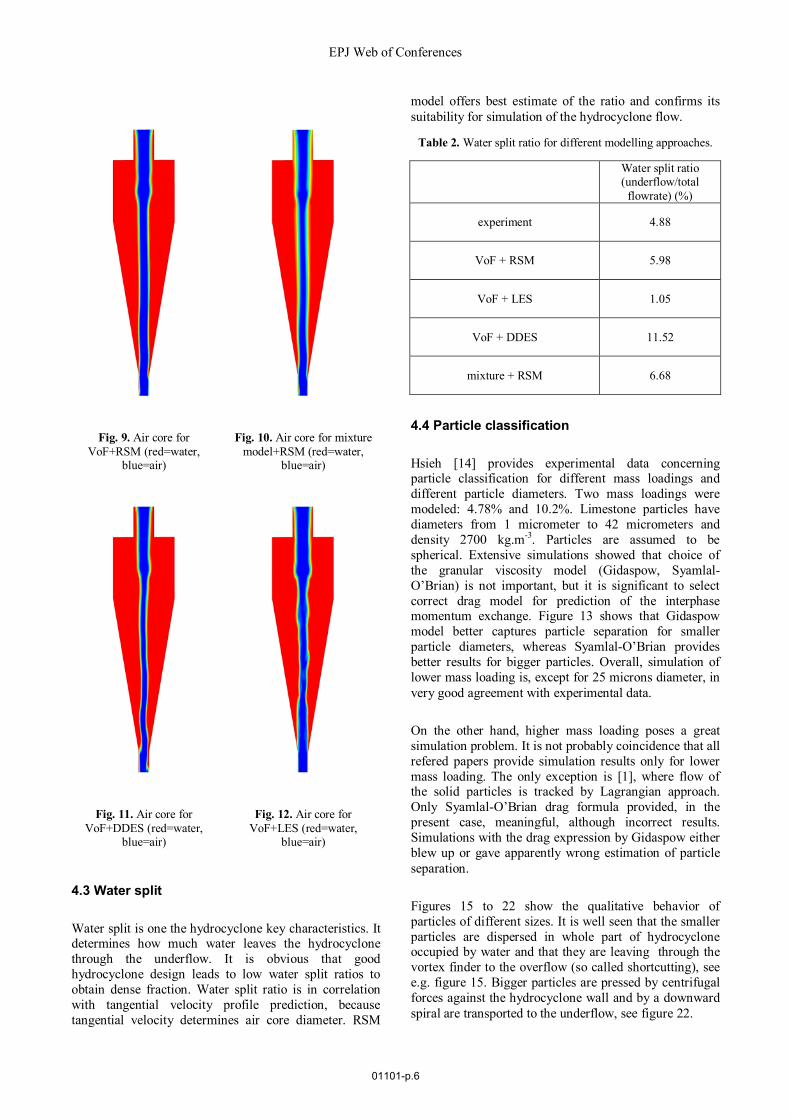
4.2 Air core

Two-phase simulation gives information on distribution of air and water in the hydrocyclone interior. Enlargement of the air core near the top wall is caused by the presence of vortex finder. Over- and underestimation of tangential velocity profile is characterized by bigger and smaller diameter of the air core for LES and DDES respectively. Although the pictures are static, they provide qualitative information about the dynamics of the air core. It is apparent that amplitudes of the air core deflection are larger in case of DDES and LES simulations.

VoF and mixture model simulations (i.e. slip was not enabled between air and water) were based on the same equations in case of two-phase simulations. However VoF captures sharp interface between the phases, whereas in case of mixture model the interface is smeared. This feature is caused by different interpolation scheme in volume fraction equation (modified HRIC for VoF, QUICK for mixture model).

Mesh size Turbulence modeling

Multiphase flow

modeling Delgadillo

and Rajamani (2005)

162k RNG k-ε, RSM, LES

VoF+Lagrangian tracking.

Brennan (2006)

231k, 314k, 1850k, 2510k

RSM, LES VoF, mixture (3-phase)

Cokljat et al (2006) 180k RSM full Eulerian

Brennan et al (2007) 56k, 450k LES Mixture (2-

phase) Leeuwner and

Eksteen (2008)

250k, 270k RSM VoF

Kuang et al (2012)

no information RSM mixture (3-

phase)

Davailles et al (2012) 250k, 450k modified k-ε,

RSM full Eulerian

01101-p.4

EFM 2012

Fig. 3. Axial velocity profile 60 mm below the hydrocyclone top wall

Fig. 4. Axial velocity profile 120 mm below the hydrocyclone top wall

Fig. 5. Axial velocity profile 170 mm below the hydrocyclone top wall

Fig. 6. Tangential velocity profile 60 mm below the hydrocyclone top wall

Fig. 7. Tangential velocity profile 120 mm below the hydrocyclone top wall

Fig. 8. Tangential velocity profile 170 mm below the hydrocyclone top wall

01101-p.5

EPJ Web of Conferences

Fig. 11. Air core for VoF+DDES (red=water,

blue=air)

Fig. 12. Air core for VoF+LES (red=water,

blue=air)

4.3 Water split

Water split is one the hydrocyclone key characteristics. It determines how much water leaves the hydrocyclone through the underflow. It is obvious that good hydrocyclone design leads to low water split ratios to obtain dense fraction. Water split ratio is in correlation with tangential velocity profile prediction, because tangential velocity determines air core diameter. RSM

model offers best estimate of the ratio and confirms its suitability for simulation of the hydrocyclone flow.

Table 2. Water split ratio for different modelling approaches.

Water split ratio (underflow/total

flowrate) (%)

experiment 4.88

VoF + RSM 5.98

VoF + LES 1.05

VoF + DDES 11.52

mixture + RSM 6.68

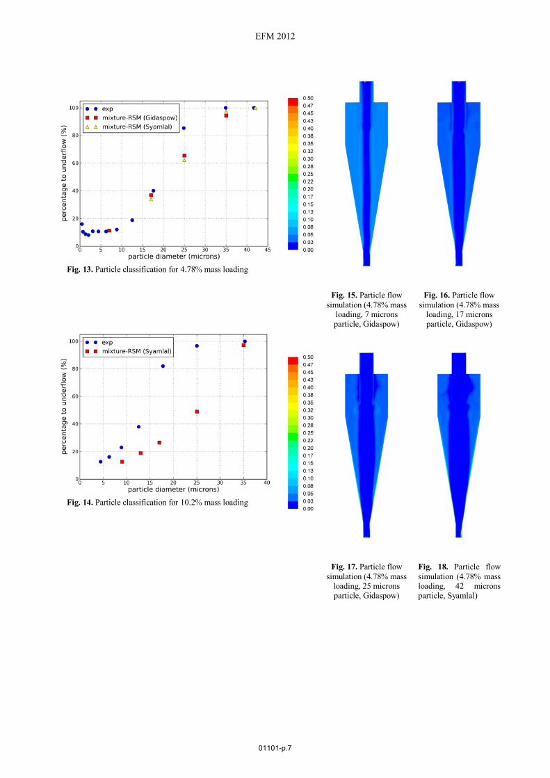
4.4 Particle classification

Hsieh [14] provides experimental data concerning particle classification for different mass loadings and different particle diameters. Two mass loadings were modeled: 4.78% and 10.2%. Limestone particles have diameters from 1 micrometer to 42 micrometers and density 2700 kg.m-3. Particles are assumed to be spherical. Extensive simulations showed that choice of the granular viscosity model (Gidaspow, Syamlal-O’Brian) is not important, but it is significant to select correct drag model for prediction of the interphase momentum exchange. Figure 13 shows that Gidaspow model better captures particle separation for smaller particle diameters, whereas Syamlal-O’Brian provides better results for bigger particles. Overall, simulation of lower mass loading is, except for 25 microns diameter, in very good agreement with experimental data.

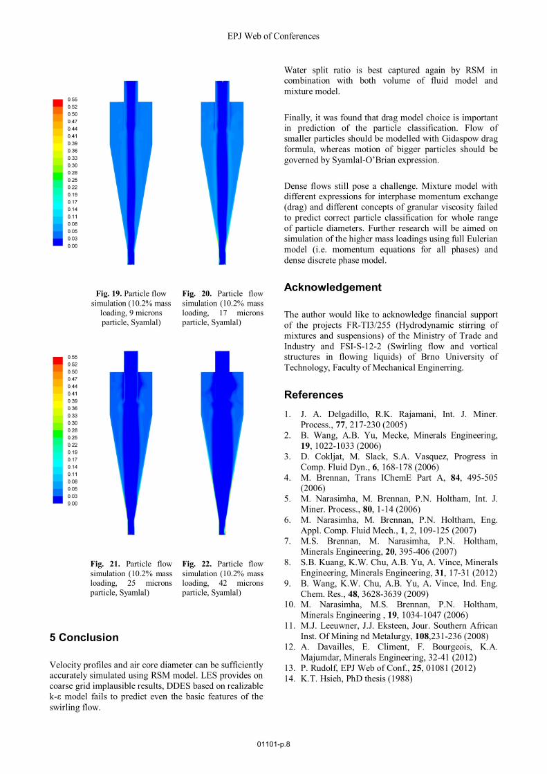
On the other hand, higher mass loading poses a great simulation problem. It is not probably coincidence that all refered papers provide simulation results only for lower mass loading. The only exception is [1], where flow of the solid particles is tracked by Lagrangian approach. Only Syamlal-O’Brian drag formula provided, in the present case, meaningful, although incorrect results. Simulations with the drag expression by Gidaspow either blew up or gave apparently wrong estimation of particle separation.

Figures 15 to 22 show the qualitative behavior of particles of different sizes. It is well seen that the smaller particles are dispersed in whole part of hydrocyclone occupied by water and that they are leaving through the vortex finder to the overflow (so called shortcutting), see e.g. figure 15. Bigger particles are pressed by centrifugal forces against the hydrocyclone wall and by a downward spiral are transported to the underflow, see figure 22.

Fig. 9. Air core for VoF+RSM (red=water,

blue=air)

Fig. 10. Air core for mixture model+RSM (red=water,

blue=air)

01101-p.6

EFM 2012

Fig. 15. Particle flow simulation (4.78% mass

loading, 7 microns particle, Gidaspow)

Fig. 16. Particle flow simulation (4.78% mass

loading, 17 microns particle, Gidaspow)

Fig. 17. Particle flow simulation (4.78% mass

loading, 25 microns particle, Gidaspow)

Fig. 18. Particle flow simulation (4.78% mass loading, 42 microns particle, Syamlal)

Fig. 13. Particle classification for 4.78% mass loading

Fig. 14. Particle classification for 10.2% mass loading

01101-p.7

EPJ Web of Conferences

Fig. 19. Particle flow simulation (10.2% mass

loading, 9 microns particle, Syamlal)

Fig. 20. Particle flow simulation (10.2% mass loading, 17 microns particle, Syamlal)

Fig. 21. Particle flow simulation (10.2% mass loading, 25 microns particle, Syamlal)

Fig. 22. Particle flow simulation (10.2% mass loading, 42 microns particle, Syamlal)

5 Conclusion

Velocity profiles and air core diameter can be sufficiently accurately simulated using RSM model. LES provides on coarse grid implausible results, DDES based on realizable k-ε model fails to predict even the basic features of the swirling flow.

Water split ratio is best captured again by RSM in combination with both volume of fluid model and mixture model.

Finally, it was found that drag model choice is important in prediction of the particle classification. Flow of smaller particles should be modelled with Gidaspow drag formula, whereas motion of bigger particles should be governed by Syamlal-O’Brian expression.

Dense flows still pose a challenge. Mixture model with different expressions for interphase momentum exchange (drag) and different concepts of granular viscosity failed to predict correct particle classification for whole range of particle diameters. Further research will be aimed on simulation of the higher mass loadings using full Eulerian model (i.e. momentum equations for all phases) and dense discrete phase model.

Acknowledgement

The author would like to acknowledge financial support of the projects FR-TI3/255 (Hydrodynamic stirring of mixtures and suspensions) of the Ministry of Trade and Industry and FSI-S-12-2 (Swirling flow and vortical structures in flowing liquids) of Brno University of Technology, Faculty of Mechanical Enginerring.

References 1. J. A. Delgadillo, R.K. Rajamani, Int. J. Miner.

Process., 77, 217-230 (2005) 2. B. Wang, A.B. Yu, Mecke, Minerals Engineering,

19, 1022-1033 (2006) 3. D. Cokljat, M. Slack, S.A. Vasquez, Progress in

Comp. Fluid Dyn., 6, 168-178 (2006) 4. M. Brennan, Trans IChemE Part A, 84, 495-505

(2006) 5. M. Narasimha, M. Brennan, P.N. Holtham, Int. J.

Miner. Process., 80, 1-14 (2006) 6. M. Narasimha, M. Brennan, P.N. Holtham, Eng.

Appl. Comp. Fluid Mech., 1, 2, 109-125 (2007) 7. M.S. Brennan, M. Narasimha, P.N. Holtham,

Minerals Engineering, 20, 395-406 (2007) 8. S.B. Kuang, K.W. Chu, A.B. Yu, A. Vince, Minerals

Engineering, Minerals Engineering, 31, 17-31 (2012) 9. B. Wang, K.W. Chu, A.B. Yu, A. Vince, Ind. Eng.

Chem. Res., 48, 3628-3639 (2009) 10. M. Narasimha, M.S. Brennan, P.N. Holtham,

Minerals Engineering , 19, 1034-1047 (2006) 11. M.J. Leeuwner, J.J. Eksteen, Jour. Southern African

Inst. Of Mining nd Metalurgy, 108,231-236 (2008) 12. A. Davailles, E. Climent, F. Bourgeois, K.A.

Majumdar, Minerals Engineering, 32-41 (2012) 13. P. Rudolf, EPJ Web of Conf., 25, 01081 (2012) 14. K.T. Hsieh, PhD thesis (1988)

01101-p.8