Simulation of Laminar Pipe Flows

57:020 Mechanics of Fluids and Transport Processes CFD PRELAB 1

By Timur Dogan, Michael Conger, Maysam Mousaviraad, Tao Xing and Fred Stern

IIHR-Hydroscience & Engineering The University of Iowa

C. Maxwell Stanley Hydraulics Laboratory Iowa City, IA 52242-1585

1. Purpose The Purpose of CFD PreLab 1 is to teach students how to use the CFD educational interface (ANSYS), be familiar with the options in each step of CFD Process, and relate simulation results to AFD concepts. Students will simulate laminar pipe flow following the “CFD process” by an interactive step-by-step approach. Students will have “hands-on” experiences using ANSYS to compute axial velocity profile, centerline velocity, centerline pressure, and wall shear stress. Students will compare simulation results with AFD data, analyze the differences and possible numerical errors, and present results in CFD Lab 1 report.

Flow chart for “CFD Process” for pipe flow

Geometry Physics Mesh Solution Results

Pipe (ANSYS Design Modeler)

Structure (ANSYS Mesh)

Non-uniform (ANSYS Mesh)

Uniform (ANSYS Mesh)

General (ANSYS Fluent - Setup) Model (ANSYS Fluent - Setup)

Boundary Conditions

(ANSYS Fluent -Setup)

Reference Values (ANSYS Fluent -

Setup)

Laminar Turbulent

Solution Methods

(ANSYS Fluent - Solution)

Monitors (ANSYS Fluent -

Solution)

Solution Initialization

(ANSYS Fluent -Solution)

Plots (ANSYS Fluent- Results)

Graphics and Animations

(ANSYS Fluent- Results)

1

2. Simulation Design In EFD Lab 2, you conducted experimental study for turbulent pipe flow. The data you have measured will be used for CFD Lab 1. In CFD PreLab 1, simulation will be conducted only for laminar circular pipe flows, i.e. the Reynolds number is less than 2300. Reynolds number based on pipe diameter and mean inlet velocity is 654.75 in the current simulation. CFD predictions of friction factor and fully developed axial velocity profile will be compared with AFD data.

Table 1 – Geometry dimensions

Parameter Unit Value Radius of Pipe m 0.02619 Diameter of Pipe m 0.05238 Length of the Pipe m 7.62

Since the flow is axisymmetric we only need to solve the flow in a single plane from the centerline to the pipe wall. Boundary conditions need to be specified include inlet, outlet, wall, and axis, as will be described in details later. Uniform flow is specified at inlet, the flow will reach the fully developed regions after a certain distance downstream. No-slip boundary condition will be used on the wall and constant pressure for the outlet. Symmetric boundary condition will be applied on the pipe axis. Since the flow is laminar, turbulence models are not necessary. Navigation Tips

• To zoom in and out use the magnifying glass with a plus sign in it and drag, from top left to bottom right over the are you wish to zoom.

• To look at a view plane, simply click on the arrow in the coordinate system identifier in the bottom right of the screen. i.e if you wish to look at the XYplane, click on the Z Arrow.

Outlet Inlet Symmetry

Pipe Wall

Non-uniform mesh Uniform mesh

Velocity Profile

Figure 1 - Geometry

2

3. Open ANSYS Workbench 3.1. Start > All Programs > ANSYS 14.5 > Workbench 14.5

3.2. From the ANSYS Workbench home screen (Project Schematic), drag and drop the Geometry component for the Component Systems on the left side of the screen into the Project Schematic. Rename the geometry by right clicking on the down arrow of the Geometry component and selecting Rename.

3

3.3. Drag and drop two Mesh components and two Fluent components into the schematic as shown below. Rename the components as you did the geometry previously as per the as shown below. Make the connections as per below by dragging component to component.

3.4. Create a Folder on the H: Drive called CFD Pre-Lab and Lab 1. 3.5. Save the project file by clicking File > Save As… 3.6. Save the project onto the H: Drive in the folder you just created and name it CFD Pre-Lab and

Lab 1 Pipe Flow. (This will be used for both Pre-Lab 1 and Lab 1.)

4. Geometry Creation 4.1. Right click on Geometry and from the drop down menu select New Geometry…

4.2. Select Meter for unit and click OK.

4

4.3. Select the XYPlane under the Tree Outline and click New Sketch button.

4.4. Right click XYPlane and select Look at.

4.5. Select Sketching > Rectangle. Create a rectangle geometry as per below, make sure to start from the origin, the mouse arrow should change to a “P” when on the origin.

5

4.6. Select Dimensions > General. Click on top edge then click above the geometry to place the dimension. Repeat the same thing for one of the vertical edges. You should have a similar figure as per below.

4.7. Click on H1under Details View, in the bottom left of the screen, and change H1 to 7.62m. Click on V2 and change it to 0.02619m.

4.8. Concept > Surface From Sketches, select the sketch by clicking on Sketch 1 in the Tree Outline and hit Apply in the Detatils View.

6

4.9. Click Generate. This will create a surface.

4.10. File >Save Project. Save project and close the Design Modeler window.

5. Mesh Generation 5.1. From the Project Schematic right click on Mesh on the Fluid Flow (Fluent) component and

select Edit…

5.2. Right click on Mesh then select Insert > Mapped Face Meshing.

7

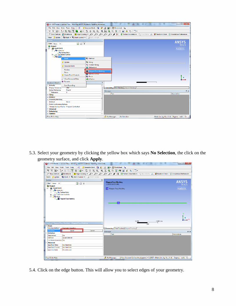
5.3. Select your geometry by clicking the yellow box which says No Selection, the click on the geometry surface, and click Apply.

5.4. Click on the edge button. This will allow you to select edges of your geometry.

8

5.5. Right click on Mesh then select Insert > Sizing.

5.6. Hold Ctrl button and select the top and bottom edge of the rectangle then click Apply. Specify details of sizing as per below in the Details of “Edge Sizing” – Sizing window.

5.7. Repeat step 5.5. Select the left and right edge of the rectangle and click Apply then change sizing parameters as per below.

9

5.8. Click on Generate Mesh button. Click Mesh under Outline. The mesh should look like the mesh pictured below.

5.9. Change the edge names by selecting the edge, then right clicking on the edge and selecting Create Named Selection. Name left, right, bottom and top edges as inlet, outlet, axis and wall respectively. Your outline should look same as the figure below.

Uniform Mesh

10

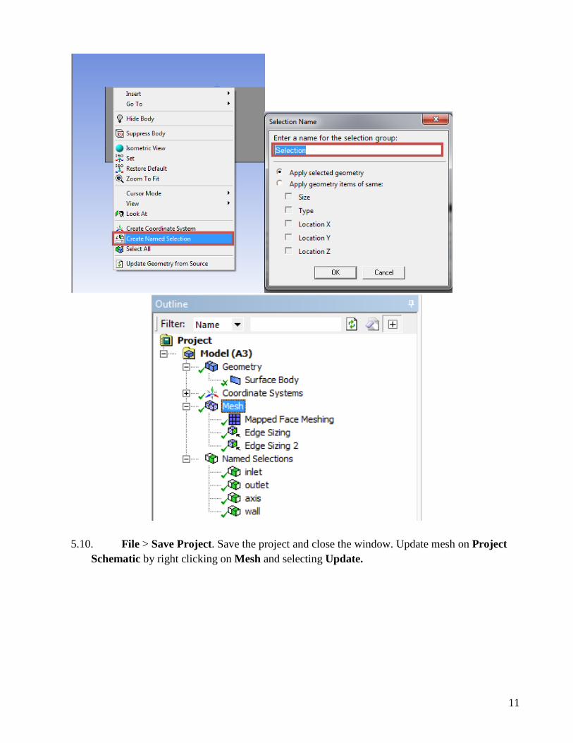
5.10. File > Save Project. Save the project and close the window. Update mesh on Project Schematic by right clicking on Mesh and selecting Update.

11

6. Setup (Physics) 6.1. Right click Setup and select Edit…

6.2. Check Double Precision and click OK.

6.3. Solution Setup > General > Check. (Note: If you get an error message you may have made a mistake while creating you mesh. Review steps in mesh generation and make changes.)

6.4. Solution Setup > General > Solver. Choose options shown below.

12

6.5. Solution Setup > Models > Edit… Make sure Laminar is selected and click OK.

13

6.6. Solution Setup > Materials > air > Create/Edit. Change the Density and Viscosity as per below and click Change/Create. Close the dialog box when finished.

6.7. Solution Setup > Cell Zone Conditions > Zone > surface_body. Change type to fluid and click OK. Select Material Name as air and click OK. This should be defaulted to fluid.

14

6.8. Solution Setup > Boundary Conditions > inlet > Edit… Change parameters as per below and click OK. Table below shows the summary of

Inlet Boundary Condition Variable u (m/s) v (m/s) P (Pa)

Magnitude 0.2 0 - Zero Gradient N N Y

15

6.9. Solution Setup > Boundary Conditions > outlet > Edit… Change parameters as per below and click OK.

Outlet Boundary Condition Variable u (m/s) v (m/s) P (Pa)

Magnitude - - 0 Zero Gradient Y Y N

6.10. Solution Setup > Boundary Conditions > wall > Edit… Change parameters as per below and click OK.

Wall Boundary Condition Variable u (m/s) v (m/s) P (Pa)

Magnitude 0 0 - Zero Gradient N N Y

16

6.11. Solution Setup > Boundary Conditions > Operating Condition. Change parameters

as per below and click OK.

17

6.12. Solution Setup > Boundary Conditions > axis. Make sure that axis is selected as per below.

Axis Boundary Condition Variable u (m/s) v (m/s) P (Pa)

Magnitude - 0 - Zero Gradient Y N Y

6.13. Solution Setup > Reference Values. Change parameters as per below.

18

7. Solution

7.1. Solution > Solution Methods. Change parameters as per below.

19

7.2. Solution > Monitors > Residuals –Print, Plot > Edit… Change convergence criterion to 1e-

06 for all three equations as per below and click OK.

7.3. Solution > Solution Initialization. Change parameters as per below and click Initialize.

20

7.4. Solution > Run Calculation. Change Number of Iterations to 1000 and click Calculate.

7.5. Once the solution converges, click OK. (The residuals should be comparable to the ones below.)

NOTE: ANSYS determines when to stop a calculation based on the iteration number and convergent limit you specified. If: 1. The maximum iteration number is reached, but convergent limit is not reached, or 2. Convergent limit is satisfied, but maximum iteration number is not reached, ANSYS will terminate the computation. File > Save Project. Save the project

21

8. Results Please read exercises before continuing.

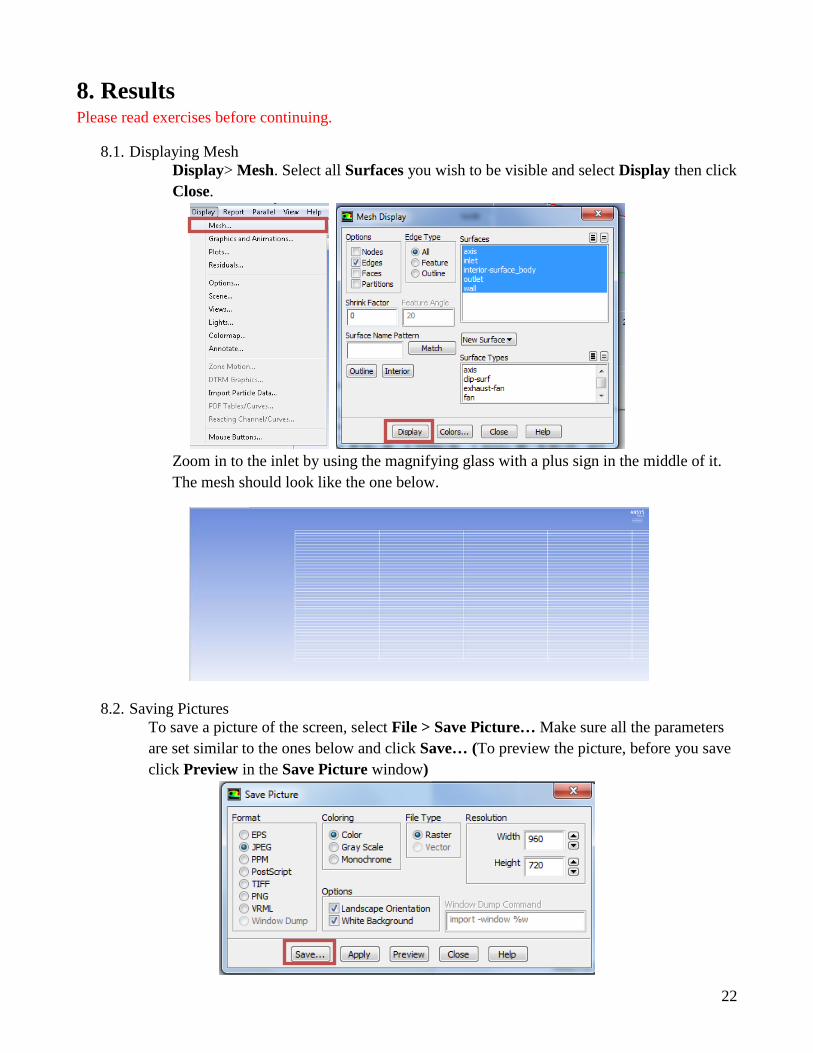
8.1. Displaying Mesh Display> Mesh. Select all Surfaces you wish to be visible and select Display then click Close.

Zoom in to the inlet by using the magnifying glass with a plus sign in the middle of it. The mesh should look like the one below.

8.2. Saving Pictures To save a picture of the screen, select File > Save Picture… Make sure all the parameters are set similar to the ones below and click Save… (To preview the picture, before you save click Preview in the Save Picture window)

22

Name the File as CFD Pre-Lab1 Laminar Pipe Flow Mesh, navigate to the CFD Pre-Lab 1 file you created and save it in that file. Then close the Save Picture window.

8.3. Displaying and Saving Residuals To display the residuals click Solution > Monitors > Residuals – Print, Plot > Edit… > Plot then click Cancel.

You can save this picture the same way you saved the mesh. Name it CFD Pre-Lab 1 Laminar Pipe Flow Residuals History and save it to the folder you created on the H: Drive.

23

8.4. Plotting and Saving Results To plot results, click Results > Plots > XY Plot > Set Up…

To plot the Centerline Pressure Distribution, copy the parameters as per below and click Plot.

Save the picture as you did for the mesh and call it CFD Pre-Lab 1 Laminar Pipe Flow Centerline Pressure Distribution and save it in the folder you created.

.

24

To plot Centerline Velocity Distribution, copy the parameters as per below and click Plot.

Save the picture as you did for the mesh and call it CFD Pre-Lab 1 Laminar Pipe Flow Centerline Velocity Distribution and save it in the folder you created.

25

To plot the Wall Shear Stress Distribution, copy the parameters as per below and click Plot.

Save the picture as you did for the mesh and call it CFD Pre-Lab 1 Laminar Pipe Flow Wall Shear Stress Distribution and save it in the folder you created.

26

To plot Profiles of Axial Velocity at All Axial Locations with AFD Data, click File > Read > Journal. Navigate to the folder you created, change Files of type to All Files and select Intro CFD Lab 1 Journal. Once selected click OK, when the Question window pops up select No. This journal creates lines at different locations along the pipe axis where velocity profile data is extracted.

Click Results > Plots > XY Plot > Set Up… Click Load File… and select axialvelocityAFD-laminar-pipe.xy, which can be found from the class website. Click OK.

27

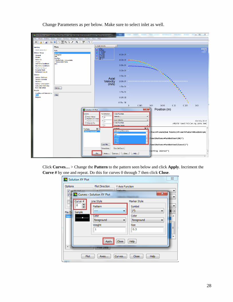
Change Parameters as per below. Make sure to select inlet as well.

Click Curves… > Change the Pattern to the pattern seen below and click Apply. Incriment the Curve # by one and repeat. Do this for curves 0 through 7 then click Close.

28

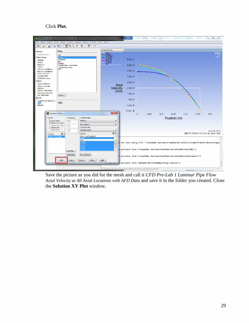
Click Plot.

Save the picture as you did for the mesh and call it CFD Pre-Lab 1 Laminar Pipe Flow Axial Velocity at All Axial Locations with AFD Data and save it in the folder you created. Close the Solution XY Plot window.

29

8.5. Plotting and Saving Graphics Click Results > Graphics and Animations > Vectors > Set Up… To plot the velocity vectors at the region flow begin to becomes fully developed, copy the parameters as per below and click Display. Zoom into the region where the flow is almost fully developed.

Save the picture as you did for the mesh and call it CFD Pre-Lab 1 Laminar Pipe Flow Velocity Vectors at the Region Flow Begins to Become Fully Developed and save it in the folder you created. Close the Vectors window.

30

Click Results > Graphics and Animations > Contours > Set Up… To plot the Contours of Radial Velocity, copy the parameters as per below and click Display. Zoom in to the pipe inlet to see the contours of radial velocity.

Save the picture as you did for the mesh and call it CFD Pre-Lab 1 Contours of Radial Velocity and save it in the folder you created. Close the Contours window.

8.6. Exporting Results To export Results, click Results > Plots > XY Plot > Set Up… To export the Developed Axial Velocity Profile at x=100d, copy the parameters as per below and click Write…

Name the file CFD Pre-Lab 1 Laminar Pipe Flow Developed Axial Velocity Profile and leave the Files of Type: as XY Files. Click OK.

31

To export the wall shear stress distribution, copy the parameters as per below and click Write…

Name the file CFD Pre-Lab 1 Laminar Pipe Flow Wall Shear Stress Distribution and leave the Files of Type: as XY Files. Click OK. Close the Solution XY Plot.

File > Save Project. Save the project and close the Fluent window.

8.7. Normalizing Velocity Profile • Open excel from Start Menu. • Click File > Open, navigate to your folder you created on the H: Drive. • Change the file type to all files. • Select the file CFD Pre-Lab 1 Laminar Pipe Flow Developed Axial Velocity Profile

and click Open. • Select Yes on the Microsoft Excel message.

• Make sure delimited is selected and click Next>. • Make sure that Tab and Space Delimiters are checked and hit Finish.

32

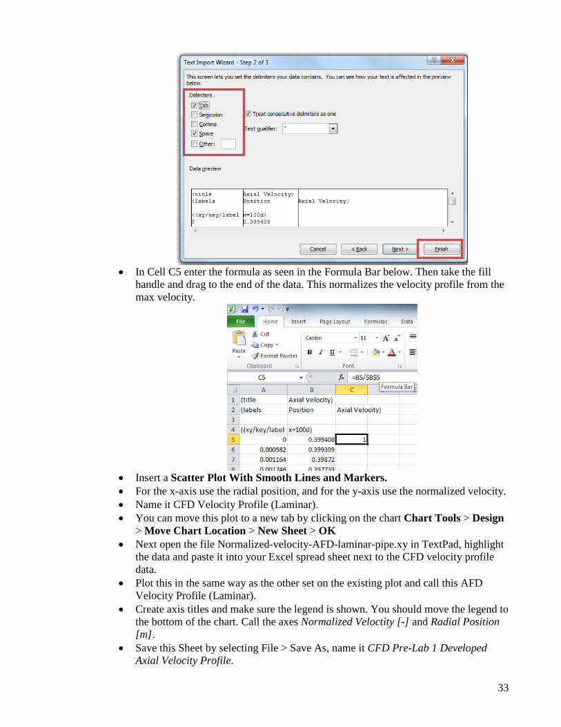
• In Cell C5 enter the formula as seen in the Formula Bar below. Then take the fill

handle and drag to the end of the data. This normalizes the velocity profile from the max velocity.

• Insert a Scatter Plot With Smooth Lines and Markers. • For the x-axis use the radial position, and for the y-axis use the normalized velocity. • Name it CFD Velocity Profile (Laminar). • You can move this plot to a new tab by clicking on the chart Chart Tools > Design

> Move Chart Location > New Sheet > OK • Next open the file Normalized-velocity-AFD-laminar-pipe.xy in TextPad, highlight

the data and paste it into your Excel spread sheet next to the CFD velocity profile data.

• Plot this in the same way as the other set on the existing plot and call this AFD Velocity Profile (Laminar).

• Create axis titles and make sure the legend is shown. You should move the legend to the bottom of the chart. Call the axes Normalized Veloctity [-] and Radial Position [m].

• Save this Sheet by selecting File > Save As, name it CFD Pre-Lab 1 Developed Axial Velocity Profile.

33

9. Exercises You must complete all the following assignments and present results in your CFD Lab 1

reports following the CFD Lab Report Instructions.

Simulation of Laminar Pipe Flow

• You need use CFD Lab1 Report Template.doc to save all the figures and data

1. Compare CFD with AFD on friction factor Use the instructions to generate the mesh and setup then iterate the simulation until it converges. Find the relative error between AFD friction factor (0.097747231) and friction factor computed by CFD, which is computed by:

100%CFD AFD

AFD

Factor FactorFactor

−×

To get the value of CFDFactor , you need first write to file the wall Shear Stress Distribution. Then use EXCEL to open the data file and pick the value close to the pipe exit or inside the fully developed region. Next use the equation C=8*τ/(ρ*U^2) to solve for the Friction Factor. Where C is the friction factor, τ is wall shear stress, ρ is density and U is the inlet velocity.

• Figures need to be saved: 1. Residual history, 2. centerline pressure distribution, 3. centerline

velocity distribution, 4. Wall shear stress distribution, 5. profiles of axial velocity at all streamwise locations (x/D=10,20,40, 60,100) with AFD data, 6. contour of radial velocity, and 7. velocity vectors (pick up the region where flow begins to become fully developed).

• Data need to be saved: shear stress in the developed region, developing length. Here, developing length is defined as the length from pipe inlet to the axial location where the centerline velocity does not change any more.

2. Normalized developed axial velocity profile

2.1. Export the axial velocity profile data at x=100d following the instructions in Step 8.6. 2.2. Use EXCEL to open the file you exported and normalize the profile using the centerline velocity magnitude, which is the maximum value on that profile. Plot the normalized velocity profile in EXCEL and paste the figure into WORD, together with other figures you made in Exercise 1.

3. Questions need to be answered when writing CFD Lab 1 report

3.1. Can you use centerline pressure distribution to determine the “developing length”? Why? 3.2. What is the value for radial velocity at developed region? 3.3. Summarize your findings in CFD Lab report and try to relate them to your classroom

lectures or textbooks.

34