Simulation of Interplanetary Trajectories Using Forward Euler Numerical Integration
15
Simulation of Interplanetary Trajectories Using Forward Euler Numerical Integration Abstract Knowledge of interplanetary trajectory mechanics is the reason that humans have been able to realize such monumental missions in space exploration. For instance, NASA’s and ESA’s joint mission, Ulysses, was the first mission to survey the space environment above and below the poles of our star. The spacecraft utilized a gravity assist maneuver of unparalleled complexity at Jupiter to shift its trajectory out of the plane of the ecliptic and into its desired solar polar orbit. This pioneering in utilization of interplanetary trajectory mechanics exposed, for the first time, the three-dimensional character of galactic cosmic radiation, energetic particles produced in solar storms, and solar wind. (Missions to our Solar System, 2013) The Ulysses mission would not have been able to achieve its solar polar orbit without utilizing the momentum of Jupiter. Even modern-day capabilities of rocket power would not have enabled Ulysses to achieve such a peculiar orbit; the efforts of conventional rocket technology alone would have been negligible in comparison to transcendental powers of planetary flyby assistance. The advantages of planetary flyby are clear; a spacecraft can essentially attain “free” changes to its velocity and trajectory direction; moreover, if the spacecraft’s trajectory is timed and positioned “perfectly”, it can strategically use its change in energy to realize such monumental missions as Ulysses. Thus, the understanding of the sensitivity of interplanetary trajectories to certain sphere of influence entry parameters is crucial. In this study, the mechanics of interplanetary trajectories are taken a closer look at through numerical analysis using Euler’s Method of numerical integration of ordinary differential equations. The objectives of this study are to establish the validity of Euler’s Method of numerical integration of ordinary differential equations with application to the gravitationally influenced motion of interplanetary trajectories, and to study the effects of the spacecraft’s velocity and position relative to its body of attraction upon its entry into the body’s sphere of influence on its interplanetary trajectory. Of course, this numerical study is conducted with observance only to values of the spacecraft’s velocity upon entry into its attracting body’s sphere of influence that are sufficiently large enough to situate the spacecraft into a hyperbolic path about the body, even for small values of the spacecraft’s position relative to the body at periapsis, such that the spacecraft will maintain the trajectory it realized upon its exiting of the body’s sphere of influence. “A spacecraft that enters a planet’s sphere of influence and does not impact the planet or go into orbit around it will continue on its hyperbolic trajectory through periapsis and exit the sphere of influence.” (Curtis, 2014)
-
Upload
christopher-iliffe-sprague -
Category
Documents
-
view
62 -
download
0
Transcript of Simulation of Interplanetary Trajectories Using Forward Euler Numerical Integration

Simulation of Interplanetary Trajectories Using Forward Euler Numerical Integration
Abstract Knowledge of interplanetary trajectory mechanics is the reason that humans have been
able to realize such monumental missions in space exploration. For instance, NASA’s and ESA’s
joint mission, Ulysses, was the first mission to survey the space environment above and below
the poles of our star. The spacecraft utilized a gravity assist maneuver of unparalleled complexity
at Jupiter to shift its trajectory out of the plane of the ecliptic and into its desired solar polar orbit.
This pioneering in utilization of interplanetary trajectory mechanics exposed, for the first time,
the three-dimensional character of galactic cosmic radiation, energetic particles produced in solar
storms, and solar wind. (Missions to our Solar System, 2013) The Ulysses mission would not
have been able to achieve its solar polar orbit without utilizing the momentum of Jupiter. Even
modern-day capabilities of rocket power would not have enabled Ulysses to achieve such a
peculiar orbit; the efforts of conventional rocket technology alone would have been negligible in
comparison to transcendental powers of planetary flyby assistance.
The advantages of planetary flyby are clear; a spacecraft can essentially attain “free”
changes to its velocity and trajectory direction; moreover, if the spacecraft’s trajectory is timed
and positioned “perfectly”, it can strategically use its change in energy to realize such
monumental missions as Ulysses. Thus, the understanding of the sensitivity of interplanetary
trajectories to certain sphere of influence entry parameters is crucial. In this study, the mechanics
of interplanetary trajectories are taken a closer look at through numerical analysis using Euler’s
Method of numerical integration of ordinary differential equations.
The objectives of this study are to establish the validity of Euler’s Method of numerical
integration of ordinary differential equations with application to the gravitationally influenced
motion of interplanetary trajectories, and to study the effects of the spacecraft’s velocity and
position relative to its body of attraction upon its entry into the body’s sphere of influence on its
interplanetary trajectory. Of course, this numerical study is conducted with observance only to
values of the spacecraft’s velocity upon entry into its attracting body’s sphere of influence that
are sufficiently large enough to situate the spacecraft into a hyperbolic path about the body, even
for small values of the spacecraft’s position relative to the body at periapsis, such that the
spacecraft will maintain the trajectory it realized upon its exiting of the body’s sphere of
influence. “A spacecraft that enters a planet’s sphere of influence and does not impact the planet
or go into orbit around it will continue on its hyperbolic trajectory through periapsis and exit the
sphere of influence.” (Curtis, 2014)

Newton’s Second Law Newton’s Second Law can be defined as
𝐹 =𝑔𝑚1𝑚2
𝑟2
For the applications of this study, it is necessary to start by defining Newton’s Second Law in
vector form
𝐹1⃗⃗ ⃗ =
𝐺𝑚1𝑚2
𝑟2�̂�
Where
𝑟 = √𝑥2 + 𝑦2
The components can be rewritten as
(𝐹𝑥 , 𝐹𝑦) = (𝐺𝑚1𝑚2
𝑥2 + 𝑦2
−𝑥
√𝑥2 + 𝑦2,𝐺𝑚1𝑚2
𝑥2 + 𝑦2
−𝑦
√𝑥2 + 𝑦2)
This yields two second-order equations that may be implemented computationally.
𝑚1𝑥′′ = −
𝐺𝑚1𝑚2𝑥
(𝑥2 + 𝑦2)3/2
𝑚1𝑦′′ = −
𝐺𝑚1𝑚2𝑦
(𝑥2 + 𝑦2)3/2
Forward Euler’s Method of Numerical Integration of Ordinary Differential Equations Forward Euler’s Method of numerical integration of ordinary differential equations may be
shown as follows
𝜔0 = 𝑦0
𝜔𝑖+1 = 𝜔𝑖 + ℎ𝑓(𝑡𝑖, 𝜔𝑖)
ℎ = 𝑡𝑖+1 − 𝑡𝑖
(Sauer, 2012)

Implementation of Forward Euler’s Method in Gravitationally Influenced Hyperbolic Trajectory of Spacecraft As the motion of the spacecraft along its hyperbolic trajectory is what is trying to be simulated, it
is necessary to define the explicit equations of the spacecraft’s acceleration in both the x-
direction and y-direction
𝑥′′ = −𝜇𝑚𝑆𝐶𝑥
(𝑥2 + 𝑦2)3/2
𝑦′′ = −𝜇𝑚𝑆𝐶𝑦
(𝑥2 + 𝑦2)3/2
These equations can be implemented in a computational context as follows
𝑡𝑖+1 = 𝑡𝑖 + ℎ
𝑣𝑥𝑖+1= 𝑣𝑥𝑖
+ ℎ𝑥′′(𝑥𝑖, 𝑥𝑖)
𝑣𝑦𝑖+1= 𝑣𝑦𝑖
+ ℎ𝑦′′(𝑥𝑖, 𝑦𝑖)
𝑥𝑖+1 = 𝑥𝑖 + ℎ𝑣𝑥𝑖
𝑦𝑖+1 = 𝑦𝑖 + ℎ𝑣𝑦𝑖
𝑟𝑖+1 = √𝑥𝑖+12 + 𝑦𝑖+1
2
It is also necessary to impose some restrictions in this simulation: the simulation is restricted
within the attracting body’s sphere of influence
𝑟 ≤ 𝑟𝑆𝑂𝐼
Moreover, the spacecraft must not crash into the surface of the attracting body
𝑟 > 𝑟𝑆𝑢𝑟𝑓
Implementation in MATLAB The iterative equations shown above may be implemented in MATLAB, or other
languages. It is necessary to specify a value for the time step, h. For this implementation in
MATLAB, “h” is now referred to as “dt”. This time step, dt, can be thought of as the resolution
of the simulation. As the value of the time step, dt, decreases, the results of simulation become
more accurate. Of course, one is limited in how small a time step can be chosen, as computation
time increases significantly.
It is also necessary to implement the imposed restrictions of the context of this study.
That is that the spacecraft must not crash into the surface of the planet, and the simulation must
stop once the spacecraft has exited the attracting body’s sphere of influence. It is also, necessary
to define the “known”. Of the knowns to be specified, there are the standard gravitational
parameter of the attracting body (𝜇), the radius of the attracting body’s sphere of influence
(𝑟𝑆𝑂𝐼), and the attracting body’s surface radius (𝑟𝑆𝑢𝑟𝑓).

For simplification in this simulation’s context, the attracting body is held stationary, so
that we may analyze the sensitivity of the spacecraft’s trajectory in accordance to its sphere of
influence entry parameters. The sphere of influence entry parameters, 𝑟𝐸𝑥 𝑎𝑛𝑑 𝑣𝐸𝑦
, are specified,
such that the entry velocity only has magnitude in the y-direction and the spacecraft’s position
coincides with the sphere of influence’s boundary. In this study, the simulation is initialized in
the coordinate systems fourth quadrant, such that the position of the attracting body is centered at
the origin. To summarize
𝑟𝐸𝑥> 0 𝑎𝑛𝑑 |𝑣𝐸| = 𝑣𝐸𝑦
Moreover, since it is desired that the spacecraft’s entry position coincide with attracting
body’s sphere of influence, it should be noted that, for the context of this simulation that
𝑟𝐸𝑦= √𝑟𝑆𝑂𝐼
2 − 𝑟𝐸𝑥2
In addition, to insure that this study only investigates hyperbolic trajectories, it was
determined through this numerical analysis that for all entry x-positions from zero to the sphere
of influence’s boundary that valid entry velocities are distinguished from the minimum value
min (𝑣𝐸𝑦) = 5
𝑘𝑚
𝑠. In this study a range of entry velocities are tested 5
𝑘𝑚
𝑠≤ 𝑣𝐸𝑦
≤ 20𝑘𝑚
𝑠.
The Forward Euler’s Method of Numerical Integration of Ordinary Differential Equations
may be implemented in a “while” loop in MATLAB as follows
%% Numerical Integration dt=10; %[s] Time step %Forward Euler Method of Numerical Ordinary Differential Equation Integration i=1; while r<=RSOIE & r>RE t(i+1)=t(i)+dt; %[s] %Next step's time vx(i+1)=vx(i)+dt*dvxdt(x(i),y(i)); %[km/s] Next step's x-velocity vy(i+1)=vy(i)+dt*dvydt(x(i),y(i)); %[km/s] Next step's y-velocity x(i+1)=x(i)+dt*dxdt(vx(i)); %[km] Next step's x-position y(i+1)=y(i)+dt*dydt(vy(i)); %[km] Next step's y-position R(i+1)=sqrt(x(i+1).^2+y(i+1).^2); %[km] Next step's distance from
Earth V(i+1)=sqrt(vx(i+1).^2+vy(i+1).^2); %[km/s] Next step's velocity psi(i+1)=atan2(y(i+1),x(i+1)); r=R(i+1); %[km] Position of spacecraft in next step i=i+1; %Change index end
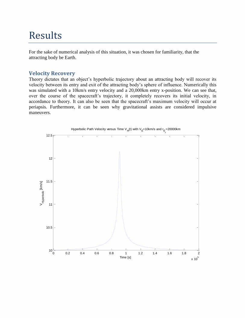
Results
For the sake of numerical analysis of this situation, it was chosen for familiarity, that the
attracting body be Earth.
Velocity Recovery Theory dictates that an object’s hyperbolic trajectory about an attracting body will recover its
velocity between its entry and exit of the attracting body’s sphere of influence. Numerically this
was simulated with a 10km/s entry velocity and a 20,000km entry x-position. We can see that,
over the course of the spacecraft’s trajectory, it completely recovers its initial velocity, in
accordance to theory. It can also be seen that the spacecraft’s maximum velocity will occur at
periapsis. Furthermore, it can be seen why gravitational assists are considered impulsive
maneuvers.
0 0.2 0.4 0.6 0.8 1 1.2 1.4 1.6 1.8 2
x 105
10
10.5
11
11.5
12
12.5
Time [s]
VH
yperb
olic
[km
/s]
Hyperbolic Path Velocity versus Time VH(t) with V
E=10km/s and r
Ex
=20000km

Anomaly with Respect to the Attracting Body It can be seen, by that act of the satellite’s hyperbolic trajectory, that its anomaly with respect to
the attracting body is changed significantly. To be clear the anomaly in this simulation is the
angle of which the spacecraft is elevated from the positive x-axis.
0 0.2 0.4 0.6 0.8 1 1.2 1.4 1.6 1.8 2
x 105
-2
-1.5
-1
-0.5
0
0.5
1
1.5
2
Angluar Position versus Time for VE=10 km/s and r
Ex
=20000 km
Time [s]
[
rad]

Entry Position’s Effect on Hyperbolic Trajectory It is evident that, as the spacecraft’s entry x-position decreases, its path deflection increases.
Notice that the satellite’s path never coincides with Earth’s radius because of the conditions
implemented in previous section’s MATLAB code. It is evident in the second plot of this
section, that the satellite’s path deflection becomes negligible as its entry x-position is moved out
toward Earth’s sphere of influence boundary.
-7 -6 -5 -4 -3 -2 -1 0 1 2
x 104
-1
0
1
2
3
4
5
6
7
x 104
rx [km]
r y [
km
]
Hyperbolic Trajectory for various rE
x
with VE=10km/s
Radius of Earth
Sphere of Influence

-1 -0.8 -0.6 -0.4 -0.2 0 0.2 0.4 0.6 0.8 1
x 106
-1
-0.8
-0.6
-0.4
-0.2
0
0.2
0.4
0.6
0.8
1x 10
6
rx [km]
r y [
km
]
Hyperbolic Trajectory with VE = 10 km/s
Radius of Earth
Sphere of Influence

-1 -0.8 -0.6 -0.4 -0.2 0 0.2 0.4 0.6 0.8 1
x 106
-1
-0.8
-0.6
-0.4
-0.2
0
0.2
0.4
0.6
0.8
1x 10
6
rx [km]
r y [
km
]
Hyperbolic Trajectory with VE = 5 km/s
Radius of Earth
Sphere of Influence

Entry Position’s Effect on Velocity at Periapsis It can be seen that as the spacecraft’s entry x-position decreases, its velocity at periapsis
increases. One should notice that the velocity at periapsis asymptotically approaches the
satellites entry velocity; again, because Earth’s gravitational influence becomes “negligible” at
its sphere of influence boundary.
1 2 3 4 5 6 7 8 9 10
x 104
10
10.5
11
11.5
12
12.5
13
13.5
14
14.5
15
Velocity at Periapsis verus Entry Position VP(r
Ex
) with VE=10km/s
rE
x
[km]
VP [
km
/s]

Hyperbolic Trajectory as a Function of Entry Position As one might predict, as the spacecraft’s entry x-position decreases, its hyperbolic path
deflection or exiting angle of trajectory relative to its entry angle of trajectory, increases. One
might be able to better understand the meaning behind the designation of an attracting body’s
sphere of influence. It can be seen from the plot that the spacecraft’s path deflection
asymptotically approaches zero. At Earth’s sphere of influence boundary the deflection of the
spacecraft’s path is “nearly’ zero; it is with this situation that astronautical engineers have
specified the boundary for which the attracting body’s gravitational pull on the spacecraft is
“negligible”.
1 2 3 4 5 6 7 8 9 10
x 104
0
0.1
0.2
0.3
0.4
0.5
0.6
0.7
0.8
Path Rotation versus Entry Position (rE
x
) with VE=10km/s
rE
x
[km]
[
rad]

Entry Velocity’s Effect on Hyperbolic Trajectory It can be seen that as the spacecraft’s entry velocity increases, its path deflection decreases. As
the spacecraft’s entry velocity increases, the attracting body has less time to pull the satellite in.
Notice, in this particular plot, the regime of this study was broken; that is, the minimum entry
velocity being analyzed is 3.5 km/s. Notice that, because of this, the minimum entry velocity’s
path was rotated by more than 90 degrees, surely not practical with such a close approach to
Earth’s surface.
-20 -15 -10 -5 0
x 104
0
2
4
6
8
10
x 104
rx [km]
r y [
km
]
Hyperbolic Trajectory for various VE with r
Ex
=20000km
Radius of Earth
Sphere of Influence

-1 -0.8 -0.6 -0.4 -0.2 0 0.2 0.4 0.6 0.8 1
x 106
-1
-0.8
-0.6
-0.4
-0.2
0
0.2
0.4
0.6
0.8
1x 10
6
rx [km]
r y [
km
]
Hyperbolic Trajectory for various Entry Velocities from 5km/s (magenta) to 20km/s (blue) with rE
x
=20000km
Radius of Earth
Sphere of Influence

Entry Velocity’s Effect on Periapsis Distance From the plot, it can be see that as the satellite’s entry velocity decreases, the satellite’s distance
of closest approach, periapsis, decreases. Note that the distance at periapsis asymptotically
approaches the spacecraft’s entry x-position. Obviously, it would be much more efficient in
terms of fuel costs to choose a greater entry x-position than to choose a higher entry velocity.
5 10 15 200.8
1
1.2
1.4
1.6
1.8
2x 10
4Periapsis Distance versus Entry Velocity r
P(V
E) with r
Ex
=20000km
VE [km/s]
r Periapsis [
km
]

Conclusion The goals of this study, to investigate entry positon’s and entry velocity’s effects on the
satellite’s hyperbolic trajectory, were realized. Indeed, the main conclusions were that decreasing
the entry velocity and decreasing the perpendicular distance from the attracting body at entry
both increased the angle by which the satellite’s hyperbolic path is rotated. To further validate
the findings of this study, it is evident from the plots that the spacecraft’s entry velocity has a
greater effect on its trajectory rotation than its perpendicular distance at entry, in accordance to
the definition of centripetal acceleration
𝑎𝑅𝑎𝑑𝑖𝑎𝑙 =𝑣𝑇𝑎𝑛𝑔𝑒𝑛𝑡𝑖𝑎𝑙
2
𝑟𝑃𝑒𝑟𝑝𝑒𝑛𝑑𝑖𝑐𝑢𝑙𝑎𝑟
It can be seen from the plots and theory, that increasing the entry velocity will increase the
spacecraft’s periapsis distance more than increasing the entry x-position will increase the
satellite’s periapsis velocity.
Future Development In the future, this code will be altered such that it will enable the analysis of gravity assist for
which the velocity of the attracting body will be nonzero. It may also be of interest to factor into
the analysis: air resistance for very close approaches, solar pressure for deep space analysis,
and/or a variable mass for the orbiting body for the application of a rocket. Further developments
may also include alteration to accommodate an n-body problem, for which the gravitational
effects of n number of bodies are accounted for.
Works Cited Curtis, H. D. (2014). Orbital Mechanics for Engineering Students. Elsevier.
Missions to our Solar System. (2013, August 15). Retrieved May 2015, from NASA:
http://solarsystem.nasa.gov/missions/profile.cfm?MCode=Ulysses
Sauer, T. (2012). Numerical Analysis. Pearson.