SIMULATION OF COMBUSTION AND THERMAL FLOW IN AN INDUSTRIAL BOILER

Raja Saripalli, Ting Wang Benjamin Day Research Assistant Professor Engineer Energy Conversion and Conservation Center Venice Natural Gas Processing Plant University of New Orleans Dynegy Midstream Services, LLP New Orleans, LA70148-2220 Venice, LA 70091

ABSTRACT Industrial boilers that produce steam or electric

power represent a crucial facility for overall plant operations. To make the boiler more efficient, less emission (cleaner) and less prone to tube rupture problems, it is important to understand the combustion and thermal flow behaviors inside the boiler. This study performs a detailed simulation of combustion and thermal flow behaviors inside an industrial boiler.

The simulations are conducted using the commercial CFD package FLUENT. The 3-D Navier-Stokes equations and five species transport equations are solved with the eddy-breakup combustion model. The simulations are conducted in three stages. In the first stage, the entire boiler is simulated without considering the steam tubes. In the second stage, a complete intensive calculation is conducted to compute the flow and heat transfer across about 496 tubes. In the third stage, the results of the saturator/superheater sections are used to calculate the thermal flow in the chimney. The results provide insight into the detailed thermal-flow and combustion in the boiler and showing possible reasons for superheater tube rupture. The exhaust gas temperature is consistent with the actual results from the infrared thermograph inspection.

INTRODUCTION Boilers [3] are commonly used in industries to

burn fuel to generate process steam and electric power. Due to economic and environmental demands, engineers are required to continuously improve the boiler efficiency and in the meantime reduce the emissions [8]. Computer simulation [2] has been employed to understand the thermal-flow and combustion phenomena in the boiler to resolve operation problems and in search for optimal solutions.

A situation may arise where the superheater tubes break due to excessive heating [9], which may lead to boiler shutdown and thus increase the expenses incurred. Overheating of the superheater tubes is prevented by using the appropriate materials and designing the unit to accommodate the heat transfer required for a given steam velocity through the superheater tubes, based on the desired exit temperature. In real applications, however, the operation of the superheater for producing high-pressure, high-temperature steam may result in problems frequently caused by ruptured superheater tubes. The damage or rupture of the superheater tubes may be caused by many possible reasons including, galvanic corrosion, thermal contraction and expansion, composition of the combustion gases, accumulations of soot outside the pipes, accumulation of slag inside the pipe or high temperature distribution above material yield temperature and high thermal stress. The damage caused by high temperature can be minimized by providing uniform combustion and temperature distribution, keeping fouling resistance low, installation of soot-blowers to remove accumulated soot and other particulates, and optimizing the combustion conditions.

The objective of this paper is to help industry to

improve boiler’s efficiency, reduce emissions, avoid rupture of superheater tubes, and to understand the thermal flow transport in the boiler. This study employs the Computational Fluid Dynamics (CFD) scheme to provide an overall picture of what is happening within the boiler, making it easy in most cases to identify the problems and develop a solution. A CFD analysis provides fluid velocity, pressure, temperature, and species concentrations throughout the solution domain. During the analysis, the geometry of the system or boundary conditions such as inlet velocity and flow rate can be easily changed to view their effects on thermal-flow patterns or species concentration distributions. CFD can also

Proceedings of 27th Industrial Energy Technology Conference May 11-12, 2005, New Orleans, Louisiana

provide detailed parametric studies that can significantly reduce the amount of experimentation necessary to identify problems and to optimize the operating conditions. However, it must be noted that the accuracy of the simulated results depends on the accuracy of models and the resolution of computational scheme adopted. PROBLEM SETUP AND MODELING

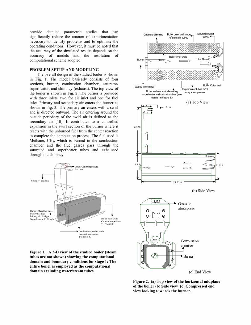
The overall design of the studied boiler is shown in Fig. 1. The model basically consists of four sections, burner, combustion chamber, saturator/ superheator, and chimney (exhaust). The top view of the boiler is shown in Fig. 2. The burner is provided with three inlets, two for air inlet and one for fuel inlet. Primary and secondary air enters the burner as shown in Fig. 3. The primary air enters with a swirl and is directed outward. The air entering around the outside periphery of the swirl air is defined as the secondary air [10]. It contributes to a controlled expansion in the swirl section of the burner where it reacts with the unburned fuel from the center reaction to complete the combustion process. The fuel used is Methane, CH4, which is burned in the combustion chamber and the flue gasses pass through the saturated and superheater tubes and exhausted through the chimney.

Burner: Mass flow rates Fuel: 0.855 kg/s Primary air: 6.9 kg/s Secondary air: 13.08 kg/s

Outlet: Constant pressure P = 1 atm

Combustion chamber walls: Constant temperature T=526.68 K

Boiler outer walls: Constant temperature T = 526.68 K

Chimney: adiabatic

Figure 1. A 3-D view of the studied boiler (steam tubes are not shown) showing the computational domain and boundary conditions for stage 1: The entire boiler is employed as the computational domain excluding water/steam tubes.

Boiler outer wall made of saturator tubes

Boiler Outer Wall

Boiler inner walls Flame

Flue Gases

Saturated water tubes

Burner

Gases to chimney

Gases to chimney Superheater tubes 6x19

array x four passes

Boiler wall made of alternating superheater and saturator tubes (see

details in Figure 3.) (a) Top View

4 .125 ft

29.33 ft

11.8 ft 11.1 ft

22.9ft

(b) Side View

Gases to atmosphere

Combustion chamber

Burner

Drum

(c) End View

Figure 2. (a) Top view of the horizontal midplane of the boiler (b) Side view (c) Compressed end view looking towards the burner.

Prima ry Air, enters with a sw irl

Secondary Air

Fue l (metha ne)

Secondary Air

Primary Air with swirl

Fuel Inlet

Secondary Air

Figure 3. (a) Schematic of the burner geometry (b) Computational model of the 3-D view of the burner exit.

The full three-dimensional Navier-Stokes equations are employed with five species transport equations. The problem is modeled with the following general assumptions:

1. The flow is steady and incompressible. 2. Variable fluid properties. 3. Turbulent flow. 4. Instantaneous combustion with the chemical

reaction much faster than the turbulence time scale.

5. The steam temperature is assumed as the tube wall temperature.

Governing Equations

The conservation equations for mass, momentum and energy in general form are shown below.

0)v(t =ρ⋅∇+∂ρ∂ (1)

Fg)(p)vv()v(t

rrrrr+ρ+τ⋅∇+−∇=ρ⋅∇+ρ

∂∂ (2)

Sh)veff(J jjh jTkeff))pE(V()E(

t+

⋅τ+∑−∇⋅∇=+ρ⋅∇+ρ

∂∂ rrr (3)

τ , the stress tensor is given by

⋅⋅∇−∇+∇µ=τ Iv

32)Tvv( rrr

where I is the unit tensor.

In energy equation E is given as,

2v 2phE +

ρ−=

“h” is sensible enthalpy and for incompressible flow it is given as

ρ+∑=

ph j

jY jh and

dTT

T refc j,ph j ∫=

Tref is constant taken as 298.15K (76.5oF). Sh in the energy equation (3) is the source term, which is provided by the net enthalpy formation rates from the species transport reactions. Boundary Conditions

The flow and thermal variables are defined by the boundary conditions on the boundaries of the studied model. Mass-flow inlet conditions are applied at the three inlets in the burner. Pressure outlet boundary condition is applied at the outlet and the walls are treated as constant wall temperature or adiabatic wall temperature. The walls are stationary with no-slip conditions applied on the wall surface. The detailed boundary conditions are summarized below. Fuel inlet: m& fuel=0.885 kg/s Air inlet: m& primary air = 6.9 kg/s, m& secondary air = 13.08 kg/s Outlet: Constant pressure at P = 1 bar Walls: No-slip condition: u = 0, v = 0, w = 0. Temperature:

• Walls at the surfaces inside the combustion chamber are covered by the saturating steam tubes at constant temperature, T = 526.68 K

• All the superheaters are set at the constant temperature, T = 672.03 K

• Saturators: All walls are set at T = 526.68 K • Superheater section: The tubes are

alternating between saturator (T = 526.86 K) and superheater (T = 672.03 K).

• Chimney walls: Adiabatic

The specific heat of the species is temperature dependant and is defined as a piecewise-polynomial function of temperature. The physical properties are defined for the mixture material and the constituent species.

(a)

(b)

Computational Domain In view of the complex geometry of the boiler,

the simulation is conducted in three stages.

Stage 1: In this stage of study, the computational domain includes the entire boiler but excludes water/steam tubes. The computational domain with all boundary conditions is shown in Fig. 1.

Burner

Combustion chamber walls, T=526.68 K

Alternating saturator/superheator tubes as the wall

Outlet, pressure condition

Saturator wall, T=526.68 K

Flow

Alternating saturator/superheater walls

Superheater tubes, T=672.03 K

Saturator tubes, T=526.68 K

Inner walls, T=526.68 K

Outer walls, T=526.68 K

Outlet, Pressure outlet, P= 1 bar

Flow

Drum Outer drum wall, T=526.68 K

Figure 4. (a) Computational domain for combustion chamber with boundary conditions for stage-2 study. (b) Computational sub-domain with boundary conditions for the saturating and superheating regions in stage 2 simulation.

Stage 2: In stage 2 of study, detailed simulation of the saturating and superheating regions is performed. Due to the large numbers of saturator and superheater tubes, the simulation is broken down into 33 sub-sections. Each sub-section includes 4x2x2 tubes. The geometry and boundary conditions are shown in Fig. 4. Initially only combustion chamber part section, as shown in Fig. 4(a), is modeled and simulated. The outlet profile solution (velocity, temperature and species concentrations) of the combustor section is used as the inlet profile

condition for the saturating/superheating regions (Fig. 4b). A total of 32 sub-sections of similar computational domain as shown in Fig. 4(b) are simulated. Each uses the outlet profile solution of the previous (upstream) sub-section as the inlet profile boundary condition. In this approach the inlet pressure information will be calculated and updated to satisfy overall mass and momentum conservation.

Stage 3: In this phase of study, the outlet results of stage 2 are used to calculate the flow in the chimney section. For this stage the computational domain and boundary conditions are shown in Fig. 5. The outlet profile (velocity, temperature and species concentration) solution of the last sub-section of stage 2 is taken as the inlet profile condition for this stage.

Pressure outlet condition

Velocity inlet profile condition

Constant wall temperature condition

Adiabatic wall condition

Figure 5. Computational domain with boundary conditions for the chimney section in stage-3 simulation.

Turbulence Model In view of the complex flow field in the boiler,

this study selects the standard κ-ε model due to its suitability and robustness for a wide range of wall-bound and free-shear flows. The κ-ε model is a semi-empirical model with several constants obtained from experiments. The turbulence kinetic energy, κ, and its rate of dissipation, ε, are obtained from the following transport equations:

In these equations, Gκ represents the generation of turbulence kinetic energy due to the mean velocity

kMbkjk

t

ji

i

SYGGxx

uxt

+−−++

∂∂

+∂∂

=∂∂

+∂∂ ρεκ

σµµρκρκ )()()( (4)

εκερεεκ

εε

ε

εσ

µµρερε SCbGCkGC

jxt

jxiu

ixt+−++

∂∂

+∂∂

=∂∂

+∂∂ 2

2)3(1)()()( (5)

(a)

(b)

gradients and the Reynolds stress, calculated as

i

jji xu

uuG∂

∂−=

−−−−−''ρκ .

bG represents the generation of turbulence kinetic energy due to buoyancy, calculated as

ixT

tPrt

igbG∂∂µ

β=

Prt is the turbulent Prandtl number and gi is the component of the gravitational vector in the i-th direction. For standard κ-ε model the value for Prt is set 0.85 in this study. β is the coefficient of thermal expansion and is given as

pT1

∂ρ∂

ρ−=β .

In equation (4), YM represents the contribution of the fluctuating dilatation in compressible turbulence to the overall dissipation rate, and is given as

2tM2MY ρε=

Mt is the turbulent Mach number, given as

2akMt = , where a = RTγ is the speed of sound.

The turbulent (or eddy) viscosity, µt, is computed by

combining κ and ε as, ε

κµρ=µ

2Ct

, where C1ε=

1.44, C2ε = 1.92, Cµ = 0.09, σκ = 1.0, σt = 1.3.

These constant values have been determined from experiments with air and water for fundamental turbulent shear flows including homogeneous shear flows and decaying isotropic grid turbulence. They have been found to work fairly well for a wide range of wall-bounded and free-shear flows. The initial values for κ and ε at the inlets and outlet are set as 1 m2/s2 and 1 m2/s3 respectively.

The κ-ε turbulence model used in this study is

primarily valid for turbulent core flows (i.e., the flow in the regions somewhat far from walls). Wall functions are used to make this turbulence model suitable for wall-bounded flows. The wall functions consist of the following: The law-of –the-wall for mean velocity gives

)Eyln(1U +κ

=+ (6)

where

ρτµ≡+

w

5.0Pk25.0CPU

U , µ

µρ PyPkCy

5.025.0≡+

k = von Karman constant (=0.42) E = empirical constant (=9.793) UP = mean velocity of the fluid at point P kP = turbulence kinetic energy at point P yP = distance from point P to the wall µ = dynamic viscosity of the fluid

The logarithmic law for mean velocity is valid for y+ > 30 to 60. The law-of-the-wall for temperature is given as,

)()Pr(Pr{Pr5.0])ln(1[Pr

)(Pr5.0Pr)(

225.025.0

25.025.05.025.0

++•

+

++•

+•

+

>−+++=

<+=−

≡

TctPtP

t

TPPPpPw

yyUUq

kCPEy

k

yyUq

kCy

q

kCcTTT

µ

µµ

ρ

ρρ

(7) where P is computed using the formula

−+

−

= tPrPr/007.0

e28.0114

3

rtPrP

24.9P

kf = thermal conductivity of the fluid ρ = density of fluid cp = specific heat of fluid q& = wall heat flux Tp = temperature at the cell adjacent to the wall Tw = temperature at the wall Pr = molecular Prandtl number (µcP/κf) Prt = turbulent Prandtl number (=0.85 at the wall) A = 26 (Van Driest constant) κ = 0.4187 (von Karman constant) E = 9.793 (wall function constant) Uc = mean velocity magnitude at y+ = yT

+ For κ-ε turbulence model, wall adjacent cells are considered to solve the κ-equation. The boundary condition for κ imposed at the wall is 0

n=

∂κ∂ , where

“n” is the local coordinate normal to the wall. The production of kinetic energy, Gk, and its dissipation rate, ε, at the wall-adjacent cells, which are the source terms in κ equation, are computed on the basis of equilibrium hypothesis with the assumption that the production of κ and its dissipation rate assumed to be equal in the wall-adjacent control volume. The production of κ and ε is computed as

Py5.0Pk25.0C

wwy

UwkG

µκρ

ττ=

∂∂

τ≈ (8)

Py

5.1pk75.0C

P κµ

=ε (9)

Radiation Model The Rosseland radiation model [6] is used in this

study, which is valid for medium optical thickness. In Rosseland model it is assumed that the intensity is the black-body intensity at the gas temperature. The radiative heat flux in a gray medium is approximated by the following equation

T3T16rq ∇Γσ−= (10)

where Γ is given as

)sC)sa(3(1

σ−σ+=Γ

where, a is absorption coefficient σs is scattering coefficient

Combustion Model

In this study, combustion of methane (CH4) is modeled by a one-step global reaction mechanism, assuming complete conversion of the fuel to CO2 and H2O. The complete stoichiometric combustion equation is given as:

CH4 + 2(O2 + 3.76 N2)→ CO2 + 2H2O + 7.52 N2 (11)

The methane-air mixture consists of 5 species

(CH4, CO2, H2O, O2 and N2). The mixing and transport of chemical species is modeled by solving the conservation equations describing convection, diffusion, and reaction sources for each component species. The species transport equations are solved by predicting the local mass fraction of each species, Yi, through the solution of a convection-diffusion equation for the i-th species. The species transport equation in general form is given as:

( ) ( ) iiiii SRJYYt

++⋅−∇=⋅∇+∂∂ rvνρρ (12)

where Ri is the net rate of production of species i by chemical reaction. Si is the rate of creation by addition from the dispersed phase plus any user-defined sources. iJ

r is the diffusion flux of species i,

which arises due to concentration gradients. For turbulent flows, mass diffusion flux is given as

it

tmii Y

ScDJ ∇

+−=

µρ ,

r. tSc is the turbulent

Schmidt number given as µt/ρDt , where µt is the turbulent viscosity and Dt is the turbulent diffusivity.

The reaction rate that appears as source term in equation (12) is given by the turbulence-chemistry interaction. In this study a generalized finite-rate combustion model (eddy-dissipation model ) is used

to solve the species transport equations. The eddy-dissipation model computes the rate of reaction under the assumption that chemical kinetics are fast compared to the rate at which reactants are mixed by turbulent fluctuations, and therefore, the overall rate of reaction for most fast burning fuels is controlled by turbulent mixing. The net rate of production of species i due to reaction r, Ri,r, is given by the smaller of the two given expressions below [7]:

νκε

ρν=

R,wMr,R'RY

RminAi,wMr,i'r,iR (13)

j,wMNj r,j"

P PYABi,wMr,i'r,iR

∑ ν

∑

κε

ρν= (14)

YP is the mass fraction of any product species, P YR is the mass fraction of a particular reactant, R

A is an empirical constant equal to 4.0 B is an empirical constant equal to 0.5 ν'i,r is the stoichiometric coefficient for reactant “i”

in reaction “r”. ν" j,r is the stoichiometric coefficient for product

“j” in reaction “r” In the above equations (13) and (14), the

chemical reaction rate is governed by the large-eddy mixing time scale, κ/ε, and an ignition source is not required. This is based on the assumption that the chemical reaction is much faster than the turbulence mixing time scale, so the actual chemical reaction is not important.

COMPUTATIONAL METHOD

The commercial software package Fluent (version 6.1.22) from Fluent, Inc. [4] is used in this study. FLUENT employs a control-volume-based [1, 5] technique to convert the governing equations to algebraic equations, which are solved numerically using the implicit method. In the segregated formulation, the governing equations are solved sequentially, i.e. segregated from one another. The SIMPLE algorithm [5] is used to couple the pressure and velocity and solves the pressure-correction implicitly. Second order upwind scheme is used to spatial discretization of the convective terms. The diffusion term is central-differenced with second-order accuracy.

Figure 6 illustrates the model geometry with

computational grid for the current study. In this study boundary layer is not important in the combustion chamber and exhaust chimney sections but is

important in the saturating/superheating sections. Wall function is used to link the solution variables at the near-wall cells and the corresponding quantities on the wall. The wall boundary conditions for the solution variables, including mean velocity,

temperature, species concentration, k, and ε, are all taken care of by the wall functions.

Full Boiler model w ith mesh

Superheating/saturation section model with mesh

Chimney model with mesh

Combustion chamber with end furnace wall model w ith mesh

Tubes present inside the model section

Top view section of the tubes

Figure 6. Computational model of the studied boiler showing different sections with meshes

Numerical Procedure 1. Solve the continuity, momentum and κ-ε

turbulence equation using the SIMPLE algorithm (pressure-predictor-correction method)

2. Obtain the velocity, pressure and turbulence distribution

3. Solve the energy equation and calculate the temperature distribution

4. Calculate the species production using the eddy-dissipation model

5. Transfer the species production to the source terms of the species transport equations

6. Solve the species transport equation to obtain species concentration distribution and enthalpy formation

7. Transfer the enthalpy formation energy to the source term of the energy equation

8. Update the continuity with new distribution of mass from the solution of species of transport equation (step 6)

9. Return to (1) and reiterate until convergence is achieved.

In the step (1) above, when the momentum

equations are solved, several iterations of the solution loop must be performed to obtain converged solution, which will satisfy the continuity and pressure-velocity relationship. Each iteration of the momentum equations consists of the following steps: (i) Fluid properties are updated first, based on the

current solution or on the initialized solution (ii) To obtain updated velocity field, the u, v, and w

momentum equations are solved using the current values of pressure and face mass fluxes.

(iii) Equation for the pressure correction is calculated from the continuity equation and the linearized momentum equations, since the velocities obtained from the above step may not satisfy the continuity equation.

(iv) The pressure correction equation obtained from above step is solved to obtain the necessary corrections to the pressure and velocity fields and face mass fluxes such that the continuity equation is satisfied

(v) Appropriate equations for scalars such as turbulence, energy, and species are solved using the updated values of the other variables.

(vi) The equation is checked for convergence. The above steps are continued till the convergence criteria are obtained and return to step 2 in the main loop. Convergence

The solution convergence is obtained by monitoring the continuity, momentum, energy,

turbulence and species equations separately. A convergence criterion of 10-3 is used for mass conservation, 10-6 is used for energy conservation, and 10-5 for velocities and turbulence values. The temperature distribution is determined after a converged solution is achieved. The energy conservation is made by enforcing the thermal energy transfer out of the domain equal to that of into the domain. The net transport of energy at the inlet and outlets consists of both the convection and diffusion components. Grid Sensitivity Study

Grid sensitivity study was conducted using a coarse grid (22424 grid points), a medium-density grid (95845 grid points) and a fine grid (198751 grid points) for the entire boiler. The comparisons are shown in Table 1. The differences of most parameters between the medium and fine grid are less than 1% except the average outlet temperature differs 2% and the total pressure losses differs 3.6%. Although the solution is still changing between the medium and the fine grid cases, considering the small difference, the medium density grid is used for this study to obtain results with reasonable time frame.

Variables Coarse grid (22,424)

Medium grid (95,845)

Fine grid (198,751)

Outlet average temperature (K) 730.64 736.72 732.96

Peak temperature in the domain (K) 1630 1630 1640

Total pressure losses (Pascal) 4617.61 4282.69 4132.08

Outlet mass-fraction of CH4

0 0 0

Outlet mass-fraction of O2

0.05641 0.05601 0.05589

Outlet mass-fraction of CO2

0.11286 0.11312 0.11321

Outlet mass-fraction of H2O 0.09240 0.09261 0.09269

Table 1. Grid sensitivity study

RESULTS AND DISCUSSION

This study illustrates the analysis of simulation of combustion and thermal flow behavior inside an industrial boiler. The simulation is conducted in two stages. In the first stage the entire boiler with combustion chamber and furnace is considered. The flow and temperature distribution is simulated without the inclusions of superheater and saturator tubes located amid the flow path. In the second stage of the simulation, the boiler is divided into three main sections. The first main section consists of only the combustion chamber where the fuel is burned. The

second main section which are further divided into 31 sub-sections including superheater and saturator tubes sections. The last main section consists of the chimney exhaust.

The flow distribution inside the entire boiler is simulated in the first stage of study. A mesh with approximately 95,845 grid points is used for the simulation. The grid incorporated the fuel inlet duct for injecting the natural gas, the primary inlet duct for injecting the swirling air stream and the secondary inlet duct for injecting the uniform air stream. Figure 7 shows the velocity vector distribution for the three inlets, where the primary air enters with a swirl. The swirling flow is used for enhance mixing for a complete combustion of air and fuel and for stabilizing the flame front. The swirl induces a recirculation zone along the centerline of the combustion chamber downstream from the burner outlet. The mass weighted average velocities for the three inlets are given in Table 2. The total air supplied is 19.98 kg/s, which is at 35 % more air than the stoichiometric value.

Variables Average Velocities (m/s)

Fuel Inlet 157.49 Primary Air Inlet 75.22 Secondary Air Inlet 57.95

Table 2. Average velocities at the burner inlets

(a) (b)

X Y

Z

Figure 7. Velocity vectors for the three inlets in the burner(a) 3-D velocity profile ( b) A cross-sectional view

The temperature distributions on the vertical

center-plane at x=0 and on the horizontal plane at y=0 are shown in Figs. 8 and 9, respectively. The temperature contour clearly shows the peak temperature is at about 1,630K (2,474oF) occurs at

about 1/4 of the boiler length and is less than the adiabatic flame temperature 2,226K (3,547oF) for methane combustion. Both Figs 8 and 9 show the flame propagation and the mixing and chemical reactions occurring closer to the inlet. The horizontal plane in Fig.9 shows that the hot flames turn around 180 degrees at the end and enters into the super-heater section at the right passage. This flame is at about 1,100K (1520oF), which is higher than the yield temperature of the superheater tube material (SA-213-T12, temperature of yield at 1050oF). This imposes a risk to the integrity of the superheater tube wall. Due to this high temperature flow, the first few rows of the super-heater tubes near the end furnace wall are subjected to the risk of rupture.

Figure 8. Contours of static temperature on the vertical plane at x=0

Figure 9. Contours of static temperature on the horizontal plane at y=0

Compositions of temperature distribution on different horizontal planes and vertical planes are

shown in Figs. 10 and 11, respectively. From these two figures, it can be clearly seen that the combustion starts as a ring, then propagates both inward and outward radially as well as longitudinally like a cone.

The flow-fields on the center horizontal and

vertical planes in Figs. 12 and 13 show the flow passes from the combustion chamber through the superheater section and finally through the chimney and is exhausted to the atmosphere. Figure 12 shows that the flame impinges on the combustion chamber sidewalls at 1/3 of the combustion chamber length. Figure 9 shows that the temperature of this impinging flame is about 1500K (2240oF). Care must be taken to frequently examine this hot region in the real boiler. Figure 12 shows that the flow separates at the 180-degree turn at the end. These separations will induce total pressure losses and requires more fan power to drive the flow through the boiler. Figure 13 shows the flow is characterized by a flame jet spreading over the combustion chamber surfaces, top and bottom with a temperature of about 1250K (1790oF) at about 1/3 of the chamber length. A recirculation zone is seen surrounding the flame near the burner. Figure 14 shows profile of mass-weighted average temperature at selected axial planes. It can be seen from the figure that maximum temperature is observed at about 1/3rd of the combustion chamber length.

Figure 10. Contour temperature profile distribution on different horizontal y-planes.

Figure 11. Contour temperature profile distribution on different vertical z-planes

Figure 12. Vector plot of velocity on the horizontal plane at y=0

Figure 13. Vector plot of velocity on the vertical plane at x=0

0

200

400

600

800

1000

1200

-10-8-6-4-202

Axial Distance, z (m)

Tem

pera

ture

, T (K

)

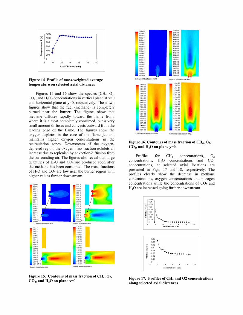
Figure 14 Profile of mass-weighted average temperature on selected axial distances

Figures 15 and 16 show the species (CH4, O2, CO2, and H2O) concentrations in vertical plane at x=0 and horizontal plane at y=0, respectively. These two figures show that the fuel (methane) is completely burned near the burner. The figures show that methane diffuses rapidly toward the flame front, where it is almost completely consumed, but a very small amount diffuses and convects outward from the leading edge of the flame. The figures show the oxygen depletes in the core of the flame jet and maintains higher oxygen concentrations in the recirculation zones. Downstream of the oxygen-depleted region, the oxygen mass fraction exhibits an increase due to replenish by advection/diffusion from the surrounding air. The figures also reveal that large quantities of H2O and CO2 are produced soon after the methane has been consumed. The mass fractions of H2O and CO2 are low near the burner region with higher values further downstream.

Figure 15. Contours of mass fraction of CH4, O2, CO2, and H2O on plane x=0

Figure 16. Contours of mass fraction of CH4, O2, CO2, and H2O on plane y=0

Profiles for CH4 concentrations, O2

concentrations, H2O concentrations and CO2 concentrations, at selected axial locations are presented in Figs. 17 and 18, respectively. The profiles clearly show the decrease in methane concentrations, oxygen concentrations and nitrogen concentrations while the concentrations of CO2 and H2O are increased going further downstream.

00.0050.010.0150.020.0250.030.0350.040.045

-10-8-6-4-202Axial Distance, z (m)

CH

4 M

ass F

ract

in

00.020.040.060.080.10.120.140.16

-10-8-6-4-202Axial Distance, z (m)

O2

Mas

s Fra

ctio

n

Figure 17. Profiles of CH4 and O2 concentrations along selected axial distances

-0.02

0

0.02

0.04

0.06

0.08

0.1

0.12

0.14

-10-8-6-4-202

Axial Distance, z (m)

CO

2 M

ass F

ract

ion

-0.02

0

0.02

0.04

0.06

0.08

0.1

0.12

-10-8-6-4-202

Axial Distance, z (m)

H2O

Mas

s Fra

ctio

n

Figure 18. Profiles of CO2 and H2O concentrations along selected axial distances.

In the second stage of this study, the second main section containing the saturator and superheater tubes is specifically zoomed in for a detailed simulation. This second main section is divided into thirty-one sub-sections. The outlet solution of the first main section (the combustion chamber) is used as the inlet condition for the first sub-section of the second main section. The first main section is simulated without downstream sections. The interface between the first and the second main sections is set at a constant pressure.

The contour temperature profile at outlet of the first section is taken as the inlet profile condition of sub-section 1 of the main second stage as shown in Fig. 19. High temperature of about 1,000K (1,340oF) is seen near the center of the flow passage. This could be the region where the material of the superheater tubes may subject to extreme high thermal load and prone to rupture. Near the inner wall, the temperature is reduced to about 970K (1,286oF) due to the separation bubble, which serves as a buffer zone to protect the inner wall from the hot flue gases.

Figure 20 shows temperature distribution on

different selected horizontal y-planes. The flow between the superheater tubes is shown in the expanded view in Fig. 20. A recirculation can be seen near the inner wall due to low pressure area created by flow separation while taking a 180 degree sharp turn from the combustion chamber to enter into the

saturator and superheater tubes section. The path lines of velocity vector colored by velocity magnitude near the superheater tubes inside the section model are shown in Fig. 21.

Figure 19. Contour temperature plot at outlet of first section of the second stage.

Figure 20. Temperature contour plots on different horizontal planes and velocity pattern on one horizontal plane.

Figure 21. Velocity vectors inside the first sub-section of the superheater section

The outlet profile conditions for velocity, temperature and species mass-fraction of sub-section 1 are taken as the inlet profile conditions for the next sub-domain (sub-section-2) and the simulation is carried until the calculation of the last sub-domain in the second main section is completed. The temperature contour plots of the entire second main section on the horizontal center-plane y = 0.3 is shown in Fig. 22. The profiles of mass-weighted average total pressure and temperature of the entire 31 sub-sections of second stage, on the horizontal plane at y=0.3 are shown in Fig. 23. The plots show decreasing temperature distribution due to heat losses to saturator and superheater tubes. The pressure drop due to the steam tubes is about 1,055Pascal (0.153psi).

C o n to u r s o f s ta t ic te m p e r a tu r e K Figure 22. Temperature contour plot of the superheater tubes section including all the 31 sub-sections on the horizontal plane at y=0.3

0

100

200

300

400

500

600

0 10 20 30 40

Axial Distance, z (m)

Pre

ssur

e, P

(Pa)

0

200

400

600

800

1000

1200

0 5 10 15 20 25 30 35

Axial Distance, -z (m)

Temp

eratur

e, T (

K)

Figure 23. Profiles of mass-weighted average total pressure and temperature of all the 31 sub-sections on the horizontal plane at y=0.3

In the third stage of study, the simulation is conducted focusing the chimney (exhaust) region. The outlet of sub-section 31 of section-2 is taken as the inlet condition for the main section-3. Peak temperature in the order of 580K (584oF) exists at the outlet of the superheater section. In the saturator section the peak temperature is lower at about 460K (368oF). This is reasonable because more energy is transferred to the saturator. Also since the saturator tube walls are maintained at a lower temperature than the superheater tube walls, the hot gasses loose more energy to the saturator tubes than to the superheater tubes. There is total pressure loss due to the saturator and superheater tubes.

The hot flue gasses loose energy to the walls

covered by saturator tubes below the steam drum and finally passing through the chimney and exhausted to the atmosphere. The temperature is reduced from about 580K (584oF) to about 465K (377oF) at the chimney exhaust (Fig. 24a). The exhaust temperature is relatively high; a fair amount of useful energy is wasted. In the actual exhaust section, an economizer is installed to recover this energy. Due to the limited scope of this study, the economizer is not considered in this study. An infrared thermography inspection of the boiler was conducted. It is interesting to see that the actual infrared image (Fig. 24b) shows the chimney exhaust gases at temperature about 461K (370oF), which are remarkably close to the CFD results at 465K (377oF).

Figure 25 shows the path lines colored by velocity magnitude. A large re-circulation zone is formed in the chimney section before leaving the atmospheric outlet. This circulation, which creates aerodynamic losses, is believed to be caused by high flow resistance due to a small exhaust opening located only on one side of the chimney walls. It is recommended that the exhaust be opened in all four walls at the end of the chimney. Figure 26 shows the vector distribution colored by temperature at selected

planes. The plot shows the flow reversal in the chimney at different horizontal planes.

Figure 24. Contour plots of static temperature at the outlet of the boiler chimney, (a) simulated results (b) infrared thermography of the boiler. Note, the color definition is different in these two figures.

CONCLUSIONS

The computational simulation of combustion and thermal-flow behavior inside an industrial boiler was performed in this study using the commercial code FLUENT. The simulations were conducted with and without considering the saturator/superheater tubes.

The results provide comprehensive information

concerning combustion and thermal-flow behavior inside an industrial boiler. The temperature distribution shows combustion starting as a ring at the interface of fuel and primary air and expanding rapidly both inwards and outwards. The flame propagates as a conical jet slightly bending toward

the roof. The hottest region is at the center of the boiler with the peak temperature around 1,630 K (2,474oF).

Figure 25. Path lines colored by velocity magnitude on z-plane

Figure 26. Velocity vector field colored by temperature on different horizontal planes

466.5

461.3

423.6

419.5

332.9

306.9

310.6273

293

313

333

353

373

393

413

433

453

473

K

The swirling flow is used to enhance the mixing of air and fuel and to stabilize the flame front. The gas flow distribution shows the flow is characterized by a flame jet spreading over the combustion chamber surface. A recirculation zones in the upper and lower portion of the combustion chamber surface near the burner are observed. The combustion and heat transfer efficiency in these recirculation zones are low. The flame impinges on the combustion chamber sidewalls at 1/3 of the combustion chamber length, with the temperature of the flame about 1,500K (2,240oF). In the vertical plane, the flame impinges on the floor and roof at about 40% of the combustion chamber length at 1,250K (1,790oF). The hot flames turn around 180 degrees at the end of the combustion chamber and enter into the superheater section. A large separation bubble forms at the turning location across a dozen rows of tubes. This separation bubble remains relatively cool at 940K (1,232oF) by entraining downstream cooler gasses. The separation bubble pushes the hot flow towards the mid-section of the passage walls and subjects the superheater tubes to high temperature thermal stress at about 1,060K (1,448oF), which can lead to tube rupture.

An intensive calculation was conducted to

compute the flow and heat transfer across the 496 tubes. With the inclusion of the saturated/super-heater tubes, the exit temperature drops from 746K (883oF) (without including saturator/super-heater tubes) to almost 465 K (377oF). The decrease in temperature is due to the heat transfer into the tubes. With the inclusion of tubes, the actual temperature distribution was simulated, and the exit temperature at the chimney exhaust is close to the actual temperature measured by infrared thermograph at about 455K (360oF). The pressure drop, due to the steam tubes, is about 1,055 Pascal (0.153 Psi).

The overall simulation was successful and

provides comprehensive information of combustion and thermal-flow in the studied boiler. Several ideas were formed from this study to improve boiler efficiency and minimize the thermal stress problem imposed on the super-heater tubes. Future work will include NOx and CO predictions. REFERENCES [1] Anderson, John D. Jr, “ Computational Fluid

Dynamics, the Basics with Application”, McGraw-Hill Inc.

[2] Armand, S and Chen, M., “A Combustion Study Of Gas Turbine Using Multi-Species/Reacting

Computational Fluid Dynamics”, Proceedings of ASME TURBO EXPO 2002, GT2002-30105.

[3] Babcock & Wilcox, “Steam its generation and

use”, 39th edition. [4] FLUENT 6.1 User’s Guide, February 2003 [5] Patankar, S.V., 1980, “Numerical Heat Transfer

and Fluid Flow”, McGraw Hill. [6] Siegel, R. and. Howell, J. R , 1992, “Thermal

Radiation Heat Transfer”, Hemisphere,Washington D.C.

[7] Turns, S. R., 2000, “An Introduction to Combustion”, 2nd Ed., McGraw Hill.

[8] Wlodzimierz, Blasiak and Yang, W., “Combustion Improvement System In Boilers and Incinerators," Proceedings of IJPGC’03, IJPGC2003-40141.

[9] Woodruff, E. B. and Lammers, H. B., “Steam Plant Operation”, McGraw-Hill,

[10] Zink, J, 2001, “The John Zink Combustion Handbook” CRC Press, New York.