Simulation Issues for Radio Detection in Ice and Salt

Amy Connolly

UCLA

May 18th, 2005

Overview

• During the past few years, simulations of Askaryan pulses and detection systems have become mature

• Large overlap in people working on simulations from GLUE, ANITA, SalSA

• This talk focuses on the status of simulations developed for ANITA, SalSA

• Lessons learned

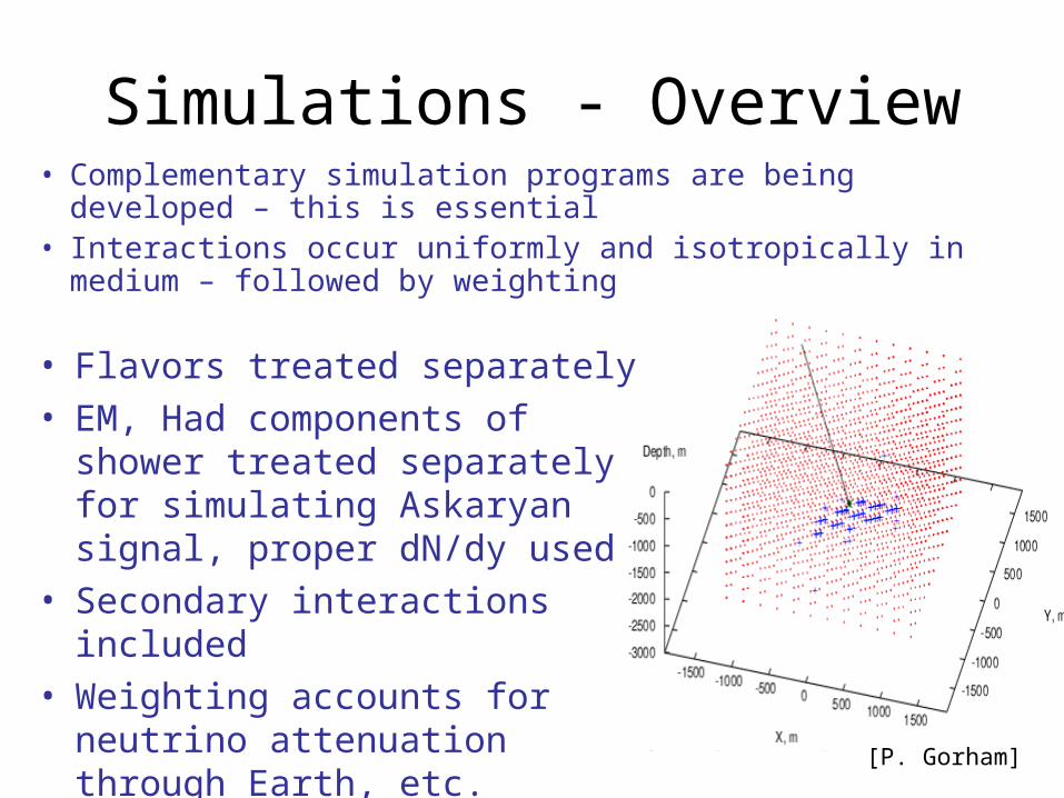
Simulations - Overview

• Flavors treated separately

• EM, Had components of shower treated separately for simulating Askaryan signal, proper dN/dy used

• Secondary interactions included

• Weighting accounts for neutrino attenuation through Earth, etc.

• Complementary simulation programs are being developed – this is essential

• Interactions occur uniformly and isotropically in medium – followed by weighting

[P. Gorham]

Anita Simulation• Ray tracing through ice, firn• Fresnel coefficients• Attenuation lengths are depth and

frequency dependent• Include surface slope and roughness• 40 quad ridged horn antennas arranged

in 3 layers: 8,8,16• Bandwidth: 200 MHz-1200 MHz• For now, signal in frequency domain• Measured antenna response

ice

[S. Barwick]

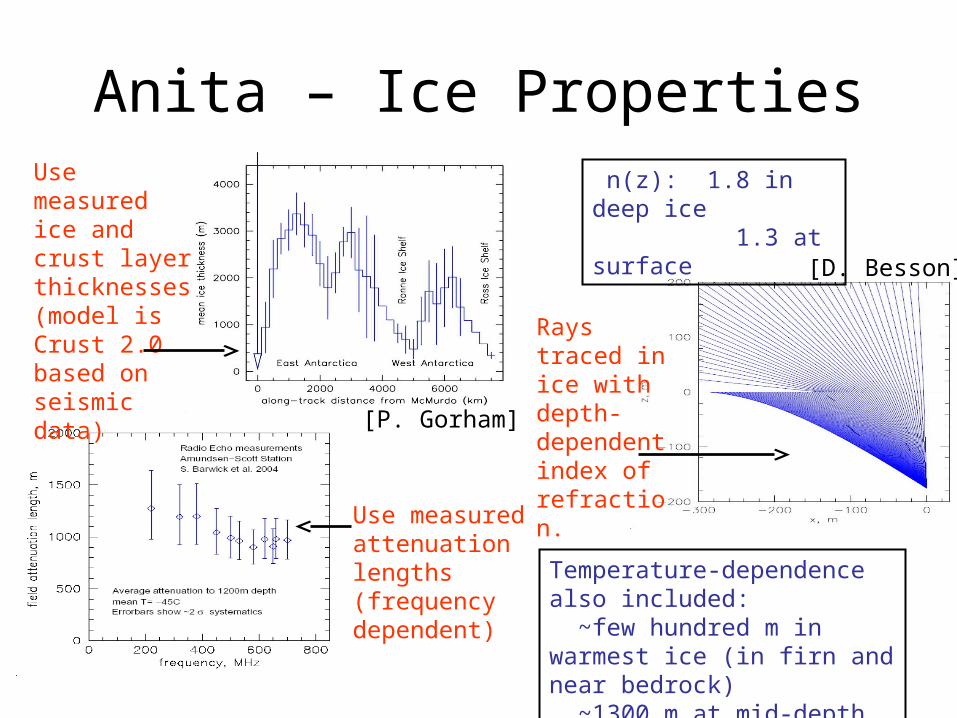
Anita – Ice PropertiesUse measured ice and crust layer thicknesses (model is Crust 2.0 based on seismic data)

Use measured attenuation lengths (frequency dependent)

Rays traced in ice with depth-dependentindex of refraction.

n(z): 1.8 in deep ice 1.3 at surface

Temperature-dependence also included: ~few hundred m in warmest ice (in firn and near bedrock) ~1300 m at mid-depth

[D. Besson]

[P. Gorham]

ANITA - Skymap

For a fixed balloon position, sensitivity on sky takes a sinusoidal shape.A source between -5 and +15 declination would be observable for 5 hrs/day

Over the entire balloon flight, sensitive to entire band between -10 and +15 declination.

Reflected RaysWork by: S. Barwick, F. Wu from University of California at Irvine

TIR

Micro-black holes at ANITA Energies

• Could measure cross section from relative rates of direct (far) to reflected (near).

[S. Barwick]

[S. Barwick &F. Wu]

• ANITA could (possibly) detect events where a signal is reflected from ice-bedrock interface

• Signals suffer from extra attenuation through ice and losses at reflection • At SM ’s, reflected rays not significant

• At large cross-sections, short pathlengths → down-going neutrinos dominate ! reflected rays important

SM

10 100 10001

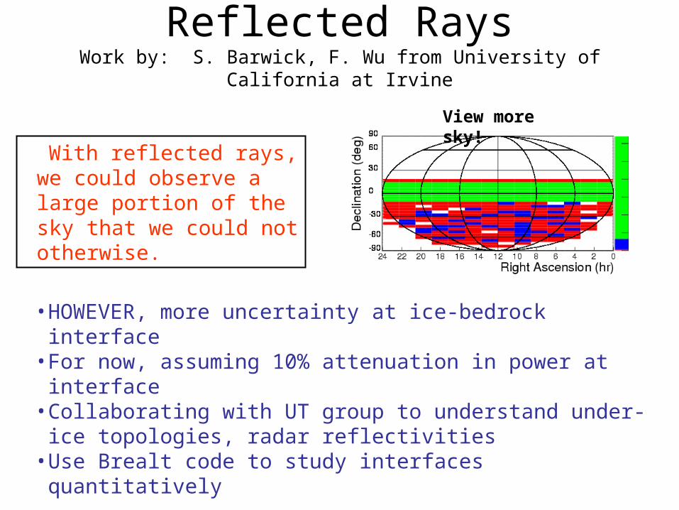
View more sky!

• HOWEVER, more uncertainty at ice-bedrock interface• For now, assuming 10% attenuation in power at interface• Collaborating with UT group to understand under-ice topologies,

radar reflectivities• Use Brealt code to study interfaces quantitatively

With reflected rays, we could observe a large portion of the sky that we could not otherwise.

Reflected RaysWork by: S. Barwick, F. Wu from University of California at Irvine

SalSA: Benchmark Detector Parameters

• Overburden: 500 m • Detector

– Array starts at 750 m below surface – 10 x 10 string square array, 250 m horiz. separation – 2000 m deep, 12 “nodes”/string, 182 m vert. separation– 12 antennas/node

• Salt extends many atten. lengths from detector walls• Attenuation length: 250 m• Alternating vert., horiz. polarization antennas• Bandwidth: 100-300 MHz• Trigger requires 5/12 antennas on node, 5 nodes to fire:

Vsignal>2.8 £ VRMS

• Index of refraction=2.45• Syst. Temp=450K=300K (salt) + 150K (receiver)

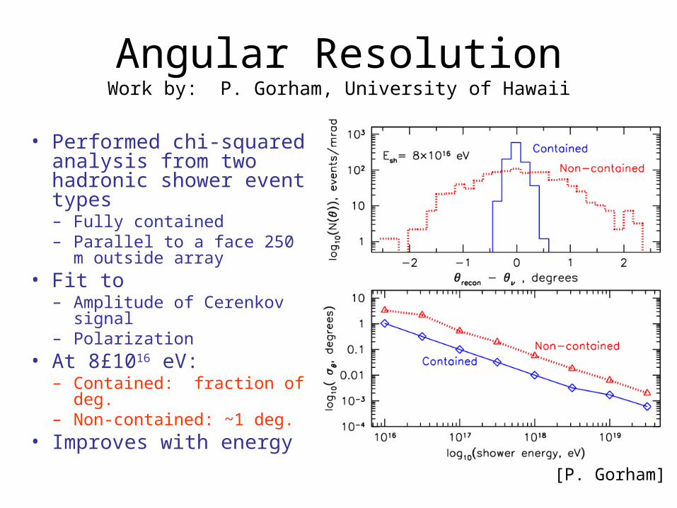
Angular ResolutionWork by: P. Gorham, University of Hawaii

[P. Gorham]

• Performed chi-squared analysis from two hadronic shower event types – Fully contained – Parallel to a face 250 m

outside array• Fit to

– Amplitude of Cerenkov signal

– Polarization• At 8£1016 eV:

– Contained: fraction of deg.– Non-contained: ~1 deg.

• Improves with energy

SalSA Cross Section Measurement

Use Poisson likelihood

cross section can be measured

from distribution

At SM , only 10% of events in sensitive region

Generate distribution from simulation and throw dice for many pseudo-experiments

For experiments w/ 100 events

With 300 events

@1018 eV,

Binning: ~2±

N

cos

<Lmeasint>=400 § 130 km

Comparing Sensitivities

ANITA:45 days

GLUE:120 hrs

RICE: 333 hrs

SalSA(1 year)

• SalSA & ANITA– SalSA lower threshold – ANITA higher V, shorter livetime

• Two independent simulations for each experiment give similar results for ES&S “baseline”– ANITA: handful of events – SalSA: 20 events/year

• Having two MC’s has been essential to:– Learn about the physics of these

systems– Spot bugs– Gain confidence in our results

ES&S “baseline”

How Do We Know Our Simulations Are Correct?

Resolving disagreement in peak at 1£1020 eV

Even if two independent simulations give the same answer, we should assume it is a coincidence until we compare many, many intermediate plots.

ANITA

Depth of Interaction (m) Balloon-to-Interaction Distance (km)

Validating our Simulations (cont)

[P. Gorham]

[S. Hoover]

ANITAProjection of Askaryan signal onto the sky:

Summary

• Simulations of radio detection systems are becoming sophisticated

• ANITA– Reflected rays show promise for detecting high cross

sections, opening up large part of the sky if ice-bedrock interface can be understood

• SALSA– Angular resolution ~fraction of degree for contained

events, 1-2 degrees for external events– Cross section measured at 30% level with 100 events

• Independent simulations are essential • Many intermediate plots necessary to verify

simulation performance

Backup Slides

ANITA

SalSA

GLUE

RICE

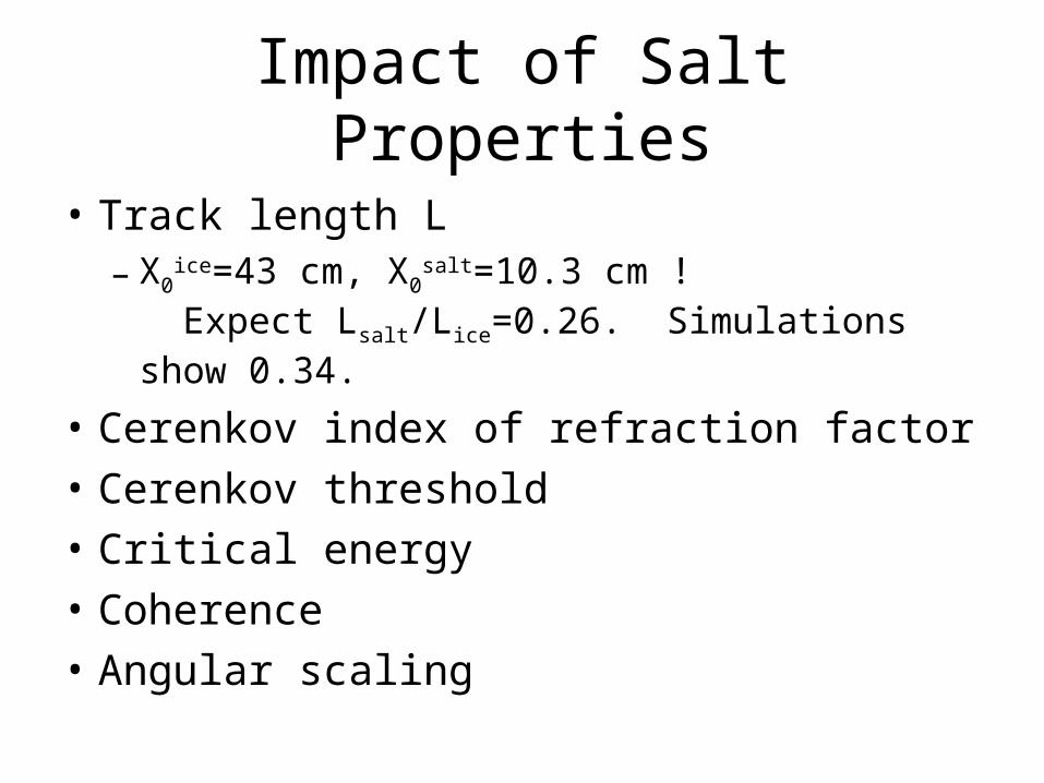
Impact of Salt Properties

• Track length L– X0

ice=43 cm, X0salt=10.3 cm ! Expect

Lsalt/Lice=0.26. Simulations show 0.34.

• Cerenkov index of refraction factor

• Cerenkov threshold

• Critical energy

• Coherence

• Angular scaling

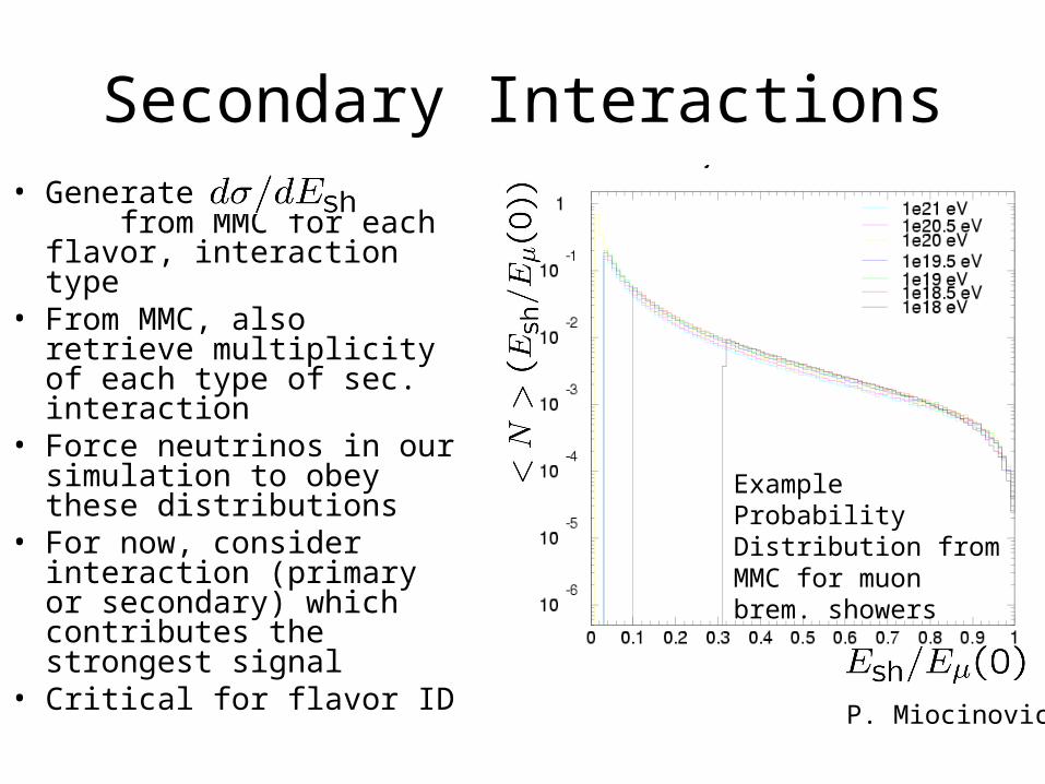
Secondary Interactions• Generate from

MMC for each flavor, interaction type

• From MMC, also retrieve multiplicity of each type of sec. interaction

• Force neutrinos in our simulation to obey these distributions

• For now, consider interaction (primary or secondary) which contributes the strongest signal

• Critical for flavor ID

Example Probability Distribution from MMC for muon brem. showers

P. Miocinovic