SIMULATION AND OPTIMIZATION OF MATERIAL FLOW FORGING DEFECTS IN AUTOMOBILE COMPONENT AND REMEDIAL...
28
SIMULATION AND OPTIMIZATION OF MATERIAL FLOW FORGING DEFECTS IN AUTOMOBILE COMPONENT AND REMEDIAL MEASURES USING DEFORM SOFTWARE SEMINAR REPORT Submitted by BENJI MATHEW VARGHESE REGISTER NO: 11003326 DEPARTMENT OF MECHANICAL ENGINEERING Believers Church Caarmel Engineering College R-Perunad, Pathanamthitta – 689 711 MAHATMA GANDHI UNIVERSITY KOTTAYAM - 686 560 NOVEMBER 2014
-
Upload
denny-john -
Category
Engineering
-
view
113 -
download
6
Transcript of SIMULATION AND OPTIMIZATION OF MATERIAL FLOW FORGING DEFECTS IN AUTOMOBILE COMPONENT AND REMEDIAL...

SIMULATION AND OPTIMIZATION OF MATERIAL FLOW
FORGING DEFECTS IN AUTOMOBILE COMPONENT AND
REMEDIAL MEASURES USING DEFORM SOFTWARE
SEMINAR REPORT
Submitted by
BENJI MATHEW VARGHESE
REGISTER NO: 11003326
DEPARTMENT OF MECHANICAL ENGINEERING
Believers Church
Caarmel Engineering College R-Perunad, Pathanamthitta – 689 711
MAHATMA GANDHI UUNNIIVVEERRSSIITTYY
KOTTAYAM - 686 560
NOVEMBER 2014
Seminar guide
Noble John Philip
Asst. Professor
Dept. of Mechanical Engg.
Caarmel Engineering College
R - Perunad
Co-ordinator
Shan James/Arun G Nath
Asst. Professor
Dept. of Mechanical Engg.
Caarmel Engineering College
R - Perunad
Head of the Department
Prof. Pramod George
Assoc. Professor
Dept. of Mechanical Engg.
Caarmel Engineering College
R - Perunad
CERTIFICATE
This is to certify that this seminar entitled
SIMULATION AND OPTIMIZATION OF MATERIAL
FLOW FORGING DEFECTS IN AUTOMOBILE COMPONENT
AND REMEDIAL MEASURES USING DEFORM SOFTWARE
was presented by
BENJI MATHEW VARGHESE
during the year 2014 in partial fulfillment of the requirement for the
award of Degree of Bachelor of Technology in Mechanical Engineering
by the
Mahatma Gandhi University.

i
ACKNOWLEDGEMENT
First of all, I thank the Almighty God for providing me the strength and courage to
present the seminar successfully.
I express my gratitude towards our Principal, Dr. Paul A.J. and the management of
our college for their support.
I use this opportunity to express my sincere gratitude towards Assoc. Prof. Pramod
George, Head of the Department of Mechanical Engineering for his valuable support,
inspiring assistance, encouragement and useful guidance. I would also like to thank Asst.
Prof. Shan James and Asst. Prof. Arun G. Nath for their valuable opinions and
corrections. I also thank my seminar guide Asst. Prof. Noble John Philip for his guidance,
support and assistance for doing my seminar in a systematic manner.
Last, but not the least, I wish to express my sincere thanks to all my friends for their
goodwill and constructive ideas and also my parents for their moral support.

ii
ABSTRACT
There are many types of defects like pitting, cracks, folds or laps, unfilling and size
variations prevalent in forging process. This paper presents the analyses of material flow
related defects with the aim of solving them using DEFORM 3D software. The main focus
is on the positioning of the billet to be kept on the bottom die and its temperature limit to
prevent the defects. A range for the positioning of the billet and temperature limit is
proposed and it is found that if the billet is kept beyond that limit, it showed the defects of
unfilling. The research is conducted on a ST 52/3 steel End plate used in automobiles, and
the results of the simulation are correlated with the Statistical results.
Key Words: DEFORM 3D, ST 52/3 Steel, Material flow, End Plate

iii
CONTENTS
Acknowledgement……………………………...……………………………………….…...i
Abstract……………………………………………………………………………………...ii
List of tables................……………………………………………………………………...iv
List of figues...........................................................................................................................v
Abbreviations……..……………………………………………………………………...…vi
Chapter 1 Introduction………………………………………………………………….…...1
Chapter 2 Problem description……………………………………………………………....3
Chapter 3 Literature review………………………………………………….……….……..4
Chapter 4 Methodology.................................................................................................….....5
Chapter 5 Numerical Simulation.............................................................................................7
5.1 DEFORM 3D Software...................................................................................…...7
5.2 Simulation of the forging of end plate....................................................................8
Chapter 6 Results and discussions......................................................…………………......10
6.1 Deform 3d simulation results............................................................…….…........10
6.1.1 Simulation results based on the change in position of workpiece..............10
6.1.2 Simulation results based on different temperatures...................................13
6.1.3 Design of experiment results...............................................….……....….14
Chapter 7 Advantages...........................……………….…………………………………..18
Chapter 8 Conclusions……………………………………………………………………..19
References………………………………………….………………………………...….…20
iv
LIST OF TABLES
Table 6.1 Results of simulation based on positioning of the workpiece on the bottom die
during forging process……......................................................................……….12
Table 6.2 Results of simulation based on different temperature of the workpiece on the
bottom die during forging process ......................................................................14
Table 6.3 Different levels of the operating parameters (X & Y) ........................................14
Table 6.4 Set of combination of these parameters at which different experiments are
performed.............................................................................................................14
Table 6.5 ANOVA results of Design of Experiments.............................................................15
Table 6.6 Values of regression coefficients calculated from MATLAB............................16

v
LIST OF FIGURES
Figure 4.1 Methodology of the process ........................…...……………………………......5
Figure 5.1 Simulation of the forging process..................................................……………...7
Figure 5.2 Meshing of the billet............................….............................................................7
Figure 5.3 End Plate...............................................................................................................8
Figure 5.4 Simulation of End Plate …..……………………………………….………...….8
Figure 6.1 Simulation of the end plate within the Range (X= -195mm, Y=170mm) ...........10
Figure 6.2 Simulation of the end plate Range (X= -195mm, Y=175mm)..............................10
Figure 6.3 Simulation of the end plate within the Range (X= -190mm, Y=170mm)............11
Figure 6.4 Simulation of the end plate Range (X= -190mm, Y=175mm) ............................11
Figure 6.5 Simulation of the end plate within the Range (X= -190mm, Y=180mm.............11
Figure 6.6 Simulation of the end plate within Range (X= -185mm, Y=175mm).................11
Figure 6.7 Simulation of the end plate beyond the Range (X= -190mm, Y=180mm) .........12
Figure 6.8 Simulation of the end plate Range (X= -185mm, Y=175mm).............................12
Figure 6.9 Simulation of end plate at 1200 °C ....................................................................13
Figure 6.10 Simulation of end plate at 1000°C ....................................................................13
Figure 6.11 Simulation of end plate at 900 °C .....................................................................13
Figure 6.12 Comparison of results of simulation and Mathematical Model .............................17

vi
ABBREVIATIONS
FEM - Finite Element Method
ANOVA - Analysis of Variance
STL - STereoLithography
AISI - American Iron and Steel Institute

CHAPTER 1
INTRODUCTION
The process of forging is concerned with the shaping of metals by the application of
compressive forces. Forging is often classified according to the temperature at which it is
performed: '"cold," "warm," or "hot" forging. Forged parts can range in weight from less than
a kilogram to 170 metric tons. Forged parts usually require further processing to achieve a
finished part. The main advantage of hot forging is that as the metal is deformed work
hardening effects are negated by the recrystallization process. Forged parts are stronger and
tougher than cast or machined parts made from the same material due to the reason that the
hammering process arranges the micro-structure of the metal so that the crystal grains get
aligned along the part profile.
Usually, the shapes of components manufactured by forging are complex; and many
defects are induced during the process of forging such as: under filling, laps and folds.
In the past, the problems were solved by seasoned technician with trial and error.
Nowadays, the finite element method (FEM) has proven its efficiency and usefulness
simulating steady and non-steady metal forming processes. Following the development of
computer technology, the commercial based forging analysis software is gradually perfect.
An algorithm for optimal design of non-isothermal metal forming processes has been
presented. The methodology is applied to optimize the preform die shape in two-stage
forging and the initial temperature of the work-piece. The authors have analyzed the changes
of structure and temperature field in process of crankshaft forging, and the rules of metal
flow are summarized, the defects formation and preventive actions were analyzed, and the
shape of blank was optimized. The authors have discussed that the forging analysis model
can minimize the testing requirements.The authors have summarized the distribution of
strains in the various regions of the part. This has been shown that friction and lubrication
increases the amount of load required in the forging process. The authors have been able to
analyze the material flow of a forging component using DEFORM™-2D. This has been
shown that the material yield can be increased by developing a flash less version of the
component using DEFORM-2D. Simulation of stresses, strains and temperature at different
regions have also been done for defect analysis Simple model for heat transfer coefficient
between work piece and dies have also been developed. Authors have also used MSC Super

Forge for simulation of the forging process .
Various authors have discussed about various factors related with FE techniques used
for forging process. However, the issues related with positioning of the billet on the bottom
die and the temperature limit for billet are not being addressed. The aim of this research is the
analysis of the material flow defects like unfilling by taking into consideration, the above
stated issues. This research would be beneficial in reducing the material flow defects.

CHAPTER 2
PROBLEM DESCRIPTION
Many types of defects like pitting, cracks, folds or laps, unfilling and size variations
prevalent in forging process. This defects can cause the product to be unfit for use. The defect
formation cannot be avoided but can be decreased by taking proper care and measurements.
As it is said prevention is better than cure, so conducting a simulation of the flow of
the material we can analyze the properties of the material and accordingly measures can be
made for improving its flow and also to avoid defects. One such method is of place a billet at
bottom portions which decrease the temperature formed due to direct flow on to the bottom.
Thus by doing this we can avoid the defects happening.
In the past, the forging defect analysis were done by skilled technician with trial and
error method. The main disadvantages of this method are different experiments have to be
performed huge material loss, large time consumption and increases cost. Finite element
softwares are used to rectify above problems.

CHAPTER 3
LITERATURE REVIEW
Zhang Z., Dai G., Wu S., Dong L., and Liu L have discussed about various factors
related with FE techniques used for forging process. However, the issues related with
positioning of the billet on the bottom die and the temperature limit for billet are not being
addressed. The aim of this research is the analysis of the material flow defects like unfilling
by taking into consideration, the above stated issues. This research would be beneficial in
reducing the material flow forging defects.
A.M. Jafarpour, A.S. Asl, R. Bihamta, have discussed about various factors related
with FE techniques used for forging process. However, the issues related with positioning of
the billet on the bottom die and the temperature limit for billet are not being addressed. The
aim of this research is the analysis of the material flow defects like unfilling by taking into
consideration, the above stated issues. This research would be beneficial in reducing the
material flow defects.
Carlos C. Antonio, Catarina F. Castro, Luisa C. Sousa, have discussed that the forging
analysis model can minimize the testing requirements and they have summarized the
distribution of strains in the various regions of the part. This has been shown that friction and
lubrication increases the amount of load required in the forging process.

CHAPTER 4
METHODOLOGY
Modelling of dies in Pro-e software
Importing the modeled drawings into
DEFORM 3D software in .STL
Setting of all the input parameters in the pre -processor module of
DEFORM 3D software.
Positioning of the billet on the
bottom die
Starting the simulation in the Simulator module
Checking the simulation for
uniformity of material flow by giving
a pause to the simulation.
No Is material flow
uniform?
Yes A
Continue Simulation
Viewing of results in the post-processor module of DEFORM 3D software
Fig. 4.1 Methodology of the process
This begins with the modeling of the dies in the 3D modelling software Pro-e. The
modelled drawings are then imported in .STL format in DEFORM 3D software. The dies are
imported in the preprocessor module of DEFORM 3D software. In this module all the input
parameters are provided. These input parameters include the material of the workpiece and
the dies, object meshing, temperature range, friction coefficient, positioning of the
workpiece. After inputting all the parameters, the simulation is started in the simulator
module. The simulation can be paused in between and we can check whether the material
flow is uniform in the die cavity or not. The results of the simulation are viewed in the post
processor module of the software. Figure 4.1 shows the methodology followed in this
process. Deform software also gives an option for fast solution processing. This product is a
well-tested, industrial simulation engine with an interface that allows the user to make use of
it to the fullest potential.

CHAPTER 5
NUMERICAL SIMULATION 5.1 DEFORM 3D SOFTWARE
The forging process generally consists of heating the billet material to a specific
temperature after which it is deformed plastically into certain shapes by applying
compressive force on the work piece (billet). At the end of the deformation process, the shape
of the die is acquired by the work piece and a desired geometry is obtained. This research
tests the forging ability of 3D Forming software package called DEFORM 3D package. The forging problem analyzed in this paper is that of a ST 52/3 steel end plate which is used
in automobile axles. In this paper various defects occurring in forging due to material flow
like laps, unfilling are analyzed with the help of simulation using DEFORMTM
3D Version 6.1. Figure 5.1 shows the simulation of the forging process on a cylindrical billet and Figure 5.2
shows the meshing of the billet. The meshing of the billet is done by the software into 12000
elements.
Fig. 5.1 Simulation of the forging process Fig. 5.2 Meshing of the billet

5.2 SIMULATION OF THE FORGING OF END PLATE As mentioned earlier, the process analyzed is that of an actual industrial production
forging. This problem was provided by R.B. Forgings Pvt. Ltd. Punjab India. The defects are
analyzed using an End Plate used in the axles of automobiles. Figure 5.3 shows the original
end plate and Figure 5.4 shows the simulation of the end plate.
Fig. 5.3 End Plate Fig. 5.4 Simulation of End Plate The defect analysis of the end plate is done by performing a number of simulations on the
HOT FORGING option in the software package DEFORM 3D v6.1 SP1.
Different Simulations are carried out using different orientations (rotational and
offset) of the work piece and optimization of the work piece is done by these simulations.
The Simulations are carried out on the basis of change in position of the workpiece and the
change in temperature of the workpiece. The logic behind the change in the position of the
workpiece is that, there is a proper range of the Position along X-axis and Position along Y-
axis (in mm) of the workpiece (initially to be kept between the dies). If the workpiece is kept
beyond that range, then the defect of partial unfilling of the final component will occur.
Different Simulations are also carried out at different temperatures (900°C, 1000°C,
and 1200°C.) The objective of these simulations is to check for the optimum temperature for
the forging process of this component. Before starting the forging process, the raw material
(billets) is kept in the furnace at 1200 °C for about one hour. Now if the billet is not kept in
the furnace for proper time, i.e. if it is taken out of the furnace after 30 or 40 minutes, then
the temperature in the workpiece upto the core does not reach 1200 °C and if the workpiece is
not heated (completely) upto an exact temperature, the material will cool down early during
the forging process and will not properly fill in the die impression. Due to this there will be
the defect of unfilling of the component. Due to the improper flow of the material, more
material will be accumulated as required, at some place in the die cavities and this will create
the final components of oversize. The results obtained by simulations are then validated
statistically using Analysis of Variance in the Statistic module of MATLAB software. A
Mathematical Model using Regression Coefficients is prepared and the results are compared.
CHAPTER 6
RESULTS AND DISCUSSIONS 6.1 DEFORM 3D SIMULATION RESULTS
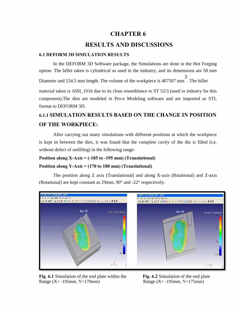
In the DEFORM 3D Software package, the Simulations are done in the Hot Forging
option. The billet taken is cylindrical as used in the industry, and its dimensions are 58 mm
Diameter and 154.5 mm length. The volume of the workpiece is 407507 mm3
. The billet
material taken is AISI_1016 due to its close resemblance to ST 52/3 (used in industry for this
component).The dies are modeled in Pro-e Modeling software and are imported as STL
format to DEFORM 3D. 6.1.1 SIMULATION RESULTS BASED ON THE CHANGE IN POSITION
OF THE WORKPIECE:
After carrying out many simulations with different positions at which the workpiece
is kept in between the dies, it was found that the complete cavity of the die is filled (i.e.
without defect of unfilling) in the following range: Position along X-Axis = (-185 to -195 mm) (Translational) Position along Y-Axis = (170 to 180 mm) (Translational)
The position along Z axis (Translational) and along X-axis (Rotational) and Z-axis
(Rotational) are kept constant as 29mm, 90° and -22° respectively.
Fig. 6.1 Simulation of the end plate within the Fig. 6.2 Simulation of the end plate Range (X= -195mm, Y=170mm) Range (X= -195mm, Y=175mm)

Figure 6.1 to Figure 6.6 shows the results of simulation of the forging when the billet is kept
in the defined range of positioning. These results show the complete filling of the die with
billet material without any defect.
Fig. 6.3 Simulation of the end plate within the within the Range (X= -190mm, Y=170mm)
Fig. 6.4 Simulation of the end plate Range (X= -190mm, Y=175mm)
Fig. 6.5 Simulation of the end plate within the Range (X= -190mm, Y=180mm)
Fig. 6.6 Simulation of the end plate within Range (X= -185mm, Y=175mm)

Simulations are also carried out by keeping the billet beyond the range defined above.
These simulations showed the defect of unfilling of the component. Figure 6.7 and Figure 6.8
shows the simulation of the forging keeping the billet beyond the range
Fig. 6.7 Simulation of the end plate beyond the Fig. 6.8 Simulation of the end plate beyond Range (X= -190mm, Y=180mm) Range (X= -185mm, Y=175mm)
Table 6.1 shows the results of simulation based on positioning of the workpiece on
the bottom die during forging process
Position along axis (mm) S No. Observation
X Y
1. -195 170 Completely Filled
2. -195 175 Completely Filled
3. -190 170 Completely Filled
4. -190 175 Completely Filled
5. -190 180 Completely Filled
6. -185 170 Completely Filled
7. -185 175 Completely Filled
8. -185 180 Completely Filled
9. -175 165 Partially Unfilled
10. -200 165 Partially Unfilled

6.1.2 SIMULATIONS RESULTS BASED ON THE DIFFERENT TEMPERATURES
Simulations are carried out at different temperatures (1200°C, 1000°C, 900°C),
keeping the other parameters constant and variations in the output are noticed. Figure 6.9
shows the simulation of the end plate at 1200 °C, the result is completely filled forging.
Figure 6.10 and 6.11 shows the unfilled components when the simulation was carried out at
1000 °C and 900 °C respectively.
Fig. 6.9 Simulation of end plate at 1200 °C Fig. 6.10 Simulation of end plate at 1000 °C Fig. 6.11 Simulation of end plate at 900 °C
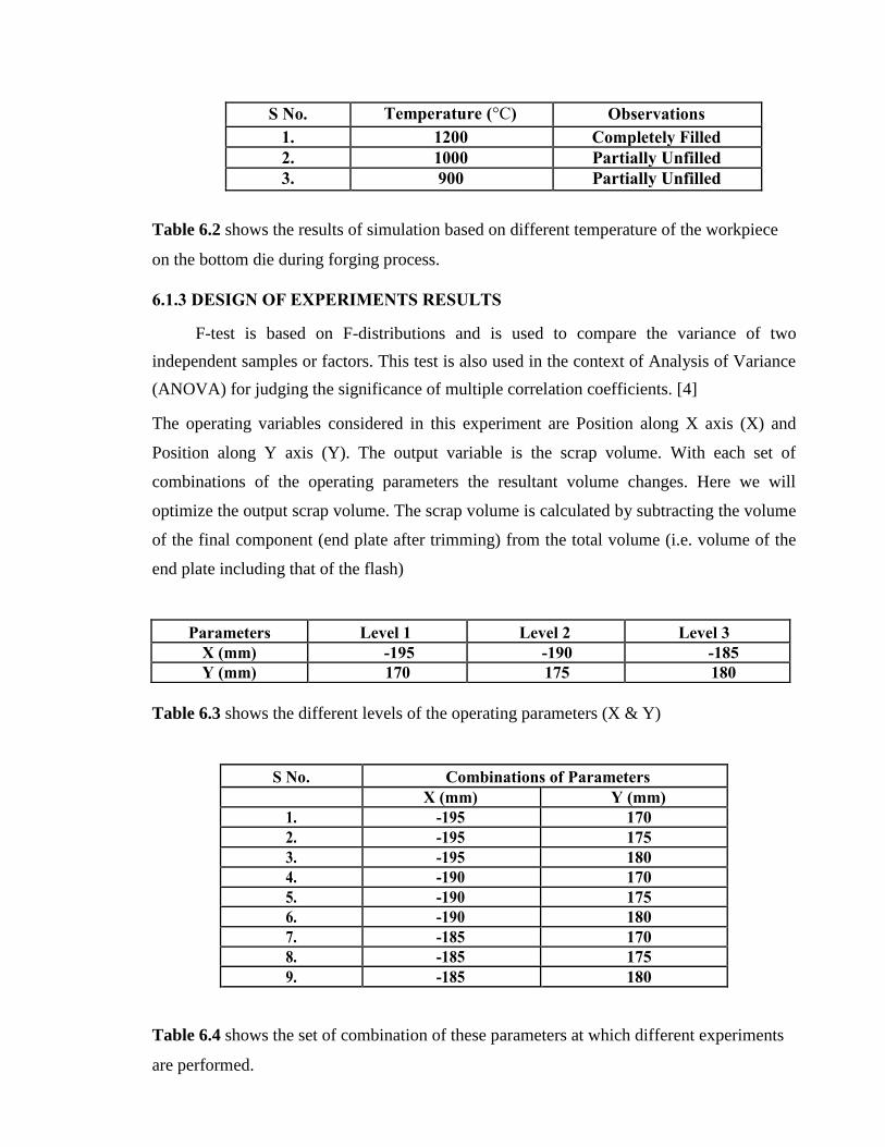
S No. Temperature (°C) Observations
1. 1200 Completely Filled
2. 1000 Partially Unfilled
3. 900 Partially Unfilled
Table 6.2 shows the results of simulation based on different temperature of the workpiece on the bottom die during forging process.
6.1.3 DESIGN OF EXPERIMENTS RESULTS
F-test is based on F-distributions and is used to compare the variance of two
independent samples or factors. This test is also used in the context of Analysis of Variance
(ANOVA) for judging the significance of multiple correlation coefficients. [4] The operating variables considered in this experiment are Position along X axis (X) and
Position along Y axis (Y). The output variable is the scrap volume. With each set of
combinations of the operating parameters the resultant volume changes. Here we will
optimize the output scrap volume. The scrap volume is calculated by subtracting the volume
of the final component (end plate after trimming) from the total volume (i.e. volume of the
end plate including that of the flash)
Table 6.3 shows the different levels of the operating parameters (X & Y)
Table 6.4 shows the set of combination of these parameters at which different experiments are performed.
Parameters Level 1 Level 2 Level 3
X (mm) -195 -190 -185
Y (mm) 170 175 180
S No. Combinations of Parameters
X (mm) Y (mm)
1. -195 170
2. -195 175
3. -195 180
4. -190 170
5. -190 175
6. -190 180
7. -185 170
8. -185 175
9. -185 180

The values input parameters are input in the MATLAB software and it generated the results
shown in Table 6.5 This ANOVA table gives the percentage contribution of the different
parameters independently and their combined effect and the error.
The results show that the %age contribution of the Position along X-axis is 10.10%,
contribution of Position along Y-axis is 35.10% and the combined contribution of Position
along X-axis and Position along Y-axis is 44.20% with 10.59% error.
Table 6.5 shows the ANOVA results of Design of Experiments
The experimental work done to study the factorial effects is planned in accordance with
the statistical techniques of the experimental design. With a well-designed experiment it is
possible to determine accurately, with a much reduced effort the effect of change in any one
variable of the process output (also known as response or yield) and the interaction effects
between the different factors if any. If all the investigated factors are quantitative in nature,
then it is possible to approximate the response Yu as a polynomial.
The mathematical model is represented in equation number 1 as:
k k
Yu = b0 + Σbi xi + Σbii xi2 i=1 i=1
+ Σb
ij xi
xj (1)
i < j
S No. Control Sum of Degree of Variance F0 %age of
Factor Squares freedom Contribution
1. A: Position 4.55813*107 2 22790700 8.58 10.1040523
along
X-axis
2. B: Position 1.58353*10 2 79176400 29.82 35.1022679 along
Y-axis
3. Interaction 1.99399*10 4 49849700 18.78 44.2009758
4. Error 4.77864*10 18 2654800 10.592859
5. Total 4.51119*10 26 100

where Xi (i = 1,2,--------k) are coded levels of K quantitative variables and b0, b1------, etc
are the least square estimates of the regression coefficients. The polynomial is also known as
Regression function and the first term under the summation sign pertains to linear effect, the
second term under the summation sign pertains to quadratic effects, and the third term
pertains to interaction effects of the investigated parameters.
The least square estimator of the regression coefficients is defined by equation 2 as:
B^
= (XT
X)T
XT
Y (2)
The values of Regression Coefficients are obtained by solving the above
equations in MATLAB software. The values of Regression Coefficients for the
given model are shown in table 6.
Table 6.6 shows the values of regression coefficients calculated from MATLAB Using the values of regression coefficients, following mathematical model is prepared for
the scrap volume. Then the results of the simulation and that of the mathematical model are
compared for validation and the results relate closely.
Equation 3 represents the mathematical model prepared for this research.
Y = 1.3622*104
+ 0.2915*104
x1 + 0.1496*104
x2 - 0.0952*104
x12 + 0.0938*104
x22 - 0.2219*104
x1x2 (3)
Regression b0 b1 b2 b11 b22 b12
Coefficients
Value 1.3622*104
0.2915*104
0.1496*104
-0.0952*104
0.0938*104
-0.2219*104

Following Graph drawn in Microsoft Excel sheet describes the comparison between the
experimental values of scrap volume, calculated by simulations and the values of scrap
volume calculated by the mathematical model.
Fig 6.12 Comparison of results of simulation and Mathematical Model

CHAPTER 7
ADVANTAGES
The main advantages of using finite element technique software such as DEFORM
3D for finding out flow forging defects are as follows.
It minimises the testing requirements for the experiments.
As there is no repetition of experiments there is no material losses taking place
and also it saves the time.
By using such softwares the exact positioning for the billet can be defined.
It reduces the experiment cost as there is no wastage of materials.
It is much accurate than that of trial and error methods so which is more
reliable.

CHAPTER 8
CONCLUSION This technique is a step forward in finding a solution to the material flow
related defects in the forging components. There are a lot of defects which are
generally seen in the forging components as described in the earlier sections.
1. In this seminar, the material flow related defects such as under fill,
over sizing of the components has been analyzed.
2. An exact range has been defined for the positioning of the billet in
between the dies. Positioning of the billet plays a very important role
in controlling the unfilling of the component. If the billet is placed
outside this range, the defect of unfilling will occur.
3. Another way of controlling these defects is by checking the proper
temperature of the billet.
Generally, before the forging of the component, the billet is heated at 1200 °C for
about an hour. This is done to heat the billet upto the core so that, when load is applied by the
forging press, the material flows easily inside the die cavity.
The actual effects of the input processes on the forging defects can be calculated. The
use of Finite Element Software like the one used in this research for these practical problems
will save a lot of time and money of the industry. In this software package, a lot of
simulations have been done to reach at a final solution. But in actual practice, if the industry
tries to reach at a optimum solution by performing different experiments on the presses, this
will cost heavily to the industry and will also consume a lot of time.

REFERENCE
1. A.M. Jafarpour, A.S. Asl, R. Bihamta, Simulation and Studying of Conical Gears
Forging, Trends in Applied Sciences Research, Academic Journals Inc. (2010) 2. Chris Wheelhouse, Dr Brian Miller, The Industrial Application of Forging Simulation At
UEF Ltd., Confederation of British Metalforming Technical Conference.
3. Deform 3D Manual, DEFORMTM
3D Version 6.1. 4. Manufacturing Technology by P.N. Rao, Tata McGraw-Hill Publishing Company Ltd.