Simulation and Multi-Objective Optimization of Road Traffic … · Dame pelo livro de contacto que...

Simulation and Multi-Objective Optimization of Road

Traffic Accidents

Paulo Ricardo Valentim Francisco

Thesis to obtain the Master of Science Degree in

Mechanical Engineering

Examination Committee

Chairperson: Doctor Luís Manuel Varejão de Oliveira Faria

Supervisors: Doctor João Manuel Pereira Dias

Doctor Luís Alberto Gonçalves de Sousa

Members of the Committee: Doctor José Firmino Aguilar Madeira

Doctor Ricardo José Fontes Portal

November 2013

i

Agradecimentos

O meu primeiro agradecimento é ao professor João Dias, por me ter acolhido à quatro

anos atrás no seu grupo, por toda a amizade e interesse que me demonstrou, por toda a

confiança que depositou em mim, por tudo aquilo que me ensinou e por tudo aquilo que me

permitiu vivenciar. Seguramente não estaria aqui hoje sem o professor.

Ao professor Luís Sousa, por toda a disponibilidade e amizade que sempre me

demostrou. E também por ter uma opinião quase sempre diferente da do Professor João Dias.

Ter duas maneiras de encarar os meus resultados permitiu-me sem dúvida melhorar o meu

trabalho.

Ao doutor Ricardo Portal, o orientador não oficial da minha tese, por todos os aspetos

referentes às formulações que discutiu comigo, pela revisão deste documento e pelas inúmeras

ideias e sugestões que me foi dando ao longo da tese. Não houve um email que eu tenha

enviado a que o Ricardo não tenha respondido.

Ao meu amigo Diogo, por toda a ajuda que me deu em aspetos de programação

(inclusive a domingos à tarde!). O seu entusiasmo pela programação aliviou muitos momentos

de “Porque é que isto está a dar erro?!”

A todos os autores contactados que tiveram a simpatia de me enviar os artigos que eu

pedi. Um agradecimento especial para o professor Nikravesh da Universidade do Arizona por

me ter digitalizado e enviado a sua informação relativo ao modelo de pneu UA Tire Model e um

agradecimento ainda mais especial ao professor Raymond Brach da Universidade de Notre

Dame pelo livro de contacto que me enviou e pela revisão e comentários à parte da minha tese

referente à modelação de contacto.

Aos meus pais, por todo o apoio que me deram ao longo dos meus anos de curso, pelo

esforço que fizeram ao longo dos anos e por terem acreditado em mim.

Finalmente, ao meu avô Rui, por todas as cópias, ditados, tabuadas, contas e problemas

que me obrigou a fazer quando eu era pequeno e voltava da escola. Agora compreendo

porquê. Também à minha avó Augusta por todos os lanchinhos depois destas sessões.

iii

Acknowledgements

My first acknowledgement is to professor João Dias, for welcoming me in is accident

investigation unit four years ago, for all his friendship and interest, for all the trust in me, for

everything he taught me and for everything he made me experience. I’d surely not be here

without him.

To professor Luís Sousa, for all the friendship and willingness to help he always

displayed me. And also for having almost always a different opinion from professor João Dias.

Having two ways of facing my results surely helped me to improve them.

To doctor Ricardo Portal, my non-official supervisor, for all the formulations he

discussed with me, for the review of this document and for the countless ideas and suggestions

he gave me throughout my master thesis. There wasn’t an e-mail sent by me that Ricardo didn’t

reply.

To my friend Diogo, for all his help regarding the programming of my codes (even on

Sunday afternoons!). His enthusiasm for programming relieved many moments of “Why isn’t this

working?!”.

To all the contacted authors who were kind enough to send me the papers I requested.

A very special thanks to Professor Nikravesh from Arizona University for his kindness to scan

and email me his information regarding the UA Tire Model and an even more special thanks to

Professor Raymond Brach from Notre Dame University for the book on contact modelling he

sent me and for the revision and insightful comments regarding the contact modelling part of my

thesis.

To my parents, for all the support they gave me throughout my college years, for their

effort and for believing in me.

Finally, to my grandfather Rui, for all the copies of texts, multiplication tables, algebra and

math problems he made me do when I was young and came back from school. Now I

understand why. Also to my grandmother Augusta for all the little snacks she made me after this

sessions.

v

Abstract

In this dissertation an innovative multi-objective optimization methodology is proposed to

tackle the traffic accident reconstruction problem. Nowadays, accident reconstructions are

carried out using trial and error methods or single-objective optimization methodologies. The

first method is very time consuming and the second one does not provide a wide range of

possible solutions, but rather converges single optimal point. The proposed multi-objective

optimization methodology minimizes two objective functions, each one representing the

difference between the rest positions obtained in the simulation and the rest positions recorded

by the police authorities, converging to a Pareto curve that provides the accident

reconstructionist an overview of multiple possible solutions. The simulation uses multibody

dynamics formulations due to its advantages when compared with the classical methods used

by most commercial software. The results so far indicate that multi-objective optimization can be

a powerful tool when applied to traffic accident reconstruction in which the process of trial and

error normally used by investigators can be replaced by a user free approach that leads to

multiple possible solutions of the problem.

Keywords:

Accident Reconstruction;

Multibody Dynamics;

Contact Detection;

Contact Force Models;

Vehicle Dynamics;

Optimization;

Multi-Objective Optimization;

Genetic Algorithms.

vii

Resumo

Nesta dissertação é proposta uma abordagem inovadora de otimização multi-objetivo

para abordar o problema da reconstituição de acidentes rodoviários. Atualmente, as

reconstituições de acidentes de viação são feitas recorrendo a métodos de tentativa e erro ou

de otimização uni-objetivo. O primeiro método é muito demorado e trabalhoso ao passo que o

segundo converge para uma única solução ótima, não fornecendo um conjunto de soluções

possíveis para o problema. A metodologia multi-objetivo proposta minimiza duas funções

objetivo, cada uma representado a diferença entre as posições finais obtidas na simulação e as

posições finais registadas pelas autoridades policiais, e converge para uma curva de Pareto,

fornecendo ao perito um conjunto de soluções possíveis para o problema. A simulação é feita

recorrendo a formulações da dinâmica de corpos múltiplos devido às suas vantagens

comparativamente aos métodos clássicos utilizados por diversos softwares comerciais. Os

resultados até ao momento indicam que a aplicação de formulações de otimização multi-

objetivo à reconstituição de acidentes rodoviários representam uma ferramenta nova e

poderosa, substituindo o processo de tentativa e erro por um processo computacional que

fornece um conjunto de soluções possíveis para o problema.

Palavras-Chave:

Reconstituição de Acidentes;

Dinâmica de Corpos Múltiplos;

Deteção de Contato;

Modelos de Força de Contato;

Dinâmica de Veículos;

Otimização;

Otimização Multi-Objetivo;

Algoritmos Genéticos.

ix

Table of Contents 1 Introduction ................................................................................................................ 1

1.1 Motivation .............................................................................................................. 1

1.2 Literature Review ................................................................................................... 4

1.2.1 Multibody Dynamics ...................................................................................... 4

1.2.2 Traffic Accident Reconstruction ..................................................................... 4

1.2.3 Multi-Objective Optimization ........................................................................ 12

1.3 Objectives and Thesis Organization .................................................................... 14

2 Multibody Dynamics Formulations .......................................................................... 15

2.1 Coordinate Systems ............................................................................................ 15

2.2 Kinematic Constraints.......................................................................................... 17

2.2.1 Spherical Joint ............................................................................................. 17

2.2.2 Revolute Joint .............................................................................................. 18

2.2.3 Cylindrical Joint ........................................................................................... 18

2.2.4 Translational Joint ....................................................................................... 19

2.3 Force Elements ................................................................................................... 19

2.3.1 Translational Springs ................................................................................... 19

2.3.2 Translational Dampers ................................................................................ 20

2.4 Contact Formulation ............................................................................................ 21

2.4.1 Surface Representation with Superellipsoids .............................................. 21

2.4.2 Broad Phase of Contact Detection .............................................................. 23

2.4.3 Narrow Phase of Contact Detection ............................................................ 27

2.5 Normal Contact-Impact Force Models ................................................................. 28

2.5.1 Nonlinear Elastic Hertz Model ..................................................................... 29

2.5.2 Nonlinear Dissipative Lankarani and Nikravesh Model ............................... 29

2.5.3 Nonlinear Dissipative Flores et al. Model .................................................... 30

2.6 Tangential Contact-Impact Force Models ........................................................... 31

2.7 Tire Model ............................................................................................................ 32

2.7.1 University of Arizona Tire Model ................................................................. 33

2.8 Equations of Motion for Unconstrained Multibody Systems ................................ 35

2.9 Equations of Motion for Constrained Multibody Systems .................................... 35

x

2.10 Solution of the Equations of Motion ................................................................. 36

3 Dynamic Simulation Results .................................................................................... 41

3.1 Bouncing Ball ....................................................................................................... 41

3.2 Multibody Model of an Automobile ...................................................................... 43

3.3 Frontal Impact Into a Rigid Wall .......................................................................... 45

3.4 Frontal Collision Between Two Vehicles ............................................................. 47

3.5 Comparison with PC-Crash Results .................................................................... 48

3.5.1 Case 1: Head-On Collision .......................................................................... 48

3.5.2 Case 2: Frontal Collision with an Offset ...................................................... 50

3.5.3 Case 3: Side Collision ................................................................................. 53

4 Multi-Objective Optimization with Genetic Algorithms ............................................. 59

4.1 Stages of a Genetic Algorithm ............................................................................. 59

4.2 Selection Operators ............................................................................................. 59

4.3 Crossover Operators ........................................................................................... 60

4.4 Mutation Operators .............................................................................................. 62

4.5 Elitism .................................................................................................................. 62

4.6 Multi-Objective Optimization ................................................................................ 62

4.7 Non-Dominated Sorting Genetic Algorithm ......................................................... 63

4.8 Application to the Traffic Accident Reconstruction Problem ............................... 65

5 Optimization of Road Traffic Accidents ................................................................... 67

5.1 Accident Reconstruction ...................................................................................... 67

5.2 The Role of Multi-Objective Optimization in Accident Reconstruction ................ 69

5.3 Application to Traffic Accident Reconstruction .................................................... 70

5.3.1 Problem Definition ....................................................................................... 70

5.3.2 Case 1: Velocity Optimization ..................................................................... 71

5.3.3 Case 2: Velocity and Heading Optimization ................................................ 74

5.3.4 Case 3: Position Optimization ..................................................................... 75

5.3.5 Case 4: Position and Velocity Optimization ................................................. 77

5.3.6 Case 5: Optimization of All Variables .......................................................... 79

5.4 Computational Aspects........................................................................................ 80

6 Conclusions and Future Developments .................................................................. 83

xi

6.1 Conclusions ......................................................................................................... 83

6.2 Future Developments .......................................................................................... 84

Bibliography ...................................................................................................................... 87

xiii

List of Figures

Figure 1.1 - Historical evolution of road traffic accidents in EU27. Source: European

Commission - Directorate General Energy and Transport (2012). ............................................... 1

Figure 1.2 - Comparison between the recorded fatalities and the targets set by the European

Commission. Source: European Commission - Directorate General Energy and Transport

(2012) and European Commission - Directorate General for Mobility and Transport (2013). ...... 2

Figure 1.3 - Comparison between the percentage of fatalities reduction and the 2001-2010

target. Source: European Commission - Directorate General for Mobility and Transport (2013) . 2

Figure 2.1 - Position of point P, according to Nikravesh (1988). ................................................. 16

Figure 2.2 - Spherical joint between two bodies. ........................................................................ 17

Figure 2.3 - Revolute joint between two bodies. ......................................................................... 18

Figure 2.4 - Cylindrical joint between two bodies. ....................................................................... 18

Figure 2.5 - Translational joint between two bodies. ................................................................... 19

Figure 2.6 - Translational spring. ................................................................................................. 20

Figure 2.7 - Translational damper. .............................................................................................. 20

Figure 2.8 - Examples of superquadric surfaces: a) Superellipsoid; b) Superhyperboloid; c)

Supertoroid. ................................................................................................................................. 21

Figure 2.9 – Influence of shape exponents in a superellipsoid with semi-axes and

semi-axis . ......................................................................................................................... 22

Figure 2.10 - Broad phase of contact detection example. .......................................................... 23

Figure 2.11 - Sphere-Sphere test: a) contact detected; b) contact not detected. Courtesy of:

Portal (2013). ............................................................................................................................... 24

Figure 2.12 - AABB test: a) contact detected; b) contact not detected. Courtesy of: Portal

(2013). ......................................................................................................................................... 24

Figure 2.13 - Separating axis test between two vehicles. ........................................................... 25

Figure 2.14 - Separating axis test (SAT) between two AABBs. Courtesy of: Portal (2013)........ 25

Figure 2.15 - OBB test: a) contact detected; b) contact not detected. Courtesy of: Portal (2013).

..................................................................................................................................................... 26

Figure 2.16 - Design variables and objective function for the optimization problem. Courtesy of:

Portal (2013). ............................................................................................................................... 28

Figure 2.17 - Nonlinear elastic Hertz model behavior: (a) normal contact force versus

penetration; (b) normal contact force and penetration versus time............................................. 29

Figure 2.18 - Nonlinear dissipative Lankarani and Nikravesh model behavior: (a) normal contact

force versus penetration; (b) normal contact force and penetration versus time. ....................... 30

Figure 2.19 - Nonlinear dissipative Flores et al. model behavior: (a) normal contact force versus

penetration; (b) normal contact force and penetration versus time............................................. 31

Figure 2.20 - Friction force models: Left - Threlfall (1978); Right - Ambrósio (2003). .............. 32

Figure 2.21 – SAE J670 reference tire frame. Courtesy of: Portal (2013). ................................. 33

Figure 2.22 - Geometric characteristics of the UA tire model. Courtesy of: Portal (2013). ......... 34

xiv

Figure 2.23 - Methodology to solve the equations of motion. ..................................................... 39

Figure 3.1 - Bouncing ball example. ............................................................................................ 41

Figure 3.2 - Bouncing ball simulation results. ............................................................................. 42

Figure 3.3 - Bouncing ball: penetration for first detected contact. ............................................... 42

Figure 3.4 - Bouncing ball: time step variation. ........................................................................... 42

Figure 3.5 - Bouncing ball: comparison of normal contact force and penetration during the first

contact period between the non-controlled and the controlled cases. ........................................ 43

Figure 3.6 - Bouncing ball: comparison of velocities during the first contact period between the

non-controlled and the controlled cases. .................................................................................... 43

Figure 3.7 - Multibody model of an automobile. .......................................................................... 44

Figure 3.8 - Frontal impact into a rigid wall: impact configuration. .............................................. 46

Figure 3.9 - Frontal impact into a rigid wall: position and velocity results. .................................. 46

Figure 3.10 - Frontal impact into a rigid wall: penetration and normal contact force results. ..... 46

Figure 3.11 - Frontal collision between two vehicles: configuration. ........................................... 47

Figure 3.12 - Frontal collision between two vehicles: position and velocity results. ................... 47

Figure 3.13 - Frontal collision between two vehicles: penetration and normal contact force

results. ......................................................................................................................................... 47

Figure 3.14 - Head-On Collision: impact configuration. .............................................................. 48

Figure 3.15 - Head-On Collision: X position results. ................................................................... 49

Figure 3.16 - Head-On Collision: X velocity results..................................................................... 49

Figure 3.17 - - Frontal Collision with an Offset: impact configuration. ........................................ 50

Figure 3.18 - Frontal Collision with an Offset: X position results. ............................................... 50

Figure 3.19 - Frontal Collision with an Offset: X velocity results. ................................................ 51

Figure 3.20 - Frontal Collision with an Offset: Y position results. ............................................... 51

Figure 3.21 - Frontal Collision with an Offset: Y velocity results. ................................................ 51

Figure 3.22 - Frontal Collision with an Offset: Angular position results. ..................................... 52

Figure 3.23 - Frontal Collision with an Offset: Angular position results. ..................................... 52

Figure 3.24 - Frontal Collision with an Offset: Angular velocity results. ...................................... 52

Figure 3.25 - Frontal Collision with Offset: maximum penetration between the vehicles (t=0.10s).

..................................................................................................................................................... 53

Figure 3.26 – Side Collision: impact configuration. ..................................................................... 53

Figure 3.27 - Side Collision: Trajectory calculated by the multibody dynamics code. ................ 54

Figure 3.28 - Side Collision: Trajectory calculated by PC-Crash. ............................................... 54

Figure 3.29 - Side Collision: X position results. ........................................................................... 54

Figure 3.30 - Side Collision: X velocity results. ........................................................................... 55

Figure 3.31 - Side Collision: Y position results. ........................................................................... 55

Figure 3.32 - Side Collision: Y velocity results. ........................................................................... 55

Figure 3.33 - Side Collision: Heading results. ............................................................................. 56

Figure 3.34 – Side Collision: Comparison between the maximum penetration obtained with PC-

Crash (t=0.90s) and the implemented multibody dynamics code (t=0.84). ................................ 57

xv

Figure 4.1 - Roulette wheel selection. ......................................................................................... 60

Figure 4.2 - Multi-Objective optimization example in the objective space (multi-dimensional

space of the objective functions). ................................................................................................ 63

Figure 4.3 - Non-dominated sorting of a population. ................................................................... 64

Figure 4.4 - Multi-objective optimization methodology. ............................................................... 65

Figure 5.1 - Accident reconstruction process. ............................................................................. 68

Figure 5.2 - Measurement Procedures: triangulation method (left) and coordinates method

(right). .......................................................................................................................................... 71

Figure 5.3 - Field Sketch: probable impact point (X) and change in skid mark direction. ........... 72

Figure 5.4 - Velocity Optimization: multi-objective optimization results (NPop=75, NGen=20). . 73

Figure 5.5 - Velocity Optimization: optimization results for two non-dominated solutions. ......... 73

Figure 5.6 - Velocity and Heading Optimization: multi-objective optimization results (NPop=75,

NGen=20). ................................................................................................................................... 74

Figure 5.7 - Velocity and Heading Optimization: optimization results for three non-dominated

solutions. ..................................................................................................................................... 75

Figure 5.8 - Position Optimization: multi-objective optimization results (NPop=75, NGen=20). . 76

Figure 5.9 - Position Optimization: optimization results for three non-dominated solutions. ...... 77

Figure 5.10 - Position and Velocity Optimization: multi-objective optimization results (NPop=75,

NGen=20). ................................................................................................................................... 78

Figure 5.11 - Position and Velocity Optimization: optimization results for three non-dominated

solutions. ..................................................................................................................................... 78

Figure 5.12 – Optimization of All Variables: multi-objective optimization results (NPop=250,

NGen=40). ................................................................................................................................... 79

Figure 5.13 – Optimization of All Variables: optimization results for four non-dominated

solutions. ..................................................................................................................................... 80

xvii

List of Tables

Table 2.1 - SAT test quantities for the AABB test. ...................................................................... 26

Table 2.2- SAT test quantities for OBB test. ............................................................................... 27

Table 3.1 - Comparison of pre and post impact states between the controlled and the non-

controlled case. ........................................................................................................................... 43

Table 3.2 - Characteristics of the vehicle. ................................................................................... 44

Table 3.3 - Geometrical and inertial properties of the elements of the multibody system. ......... 44

Table 3.4 - Characteristics of the kinematic joints....................................................................... 45

Table 3.5 - Position of the connecting points of the suspension. ................................................ 45

Table 3.6 - Parameters for the UA tire model. ............................................................................ 45

Table 3.7 - Comparison of pre and post impact state. ................................................................ 46

Table 3.8 - Comparison of pre and post impact state. ................................................................ 48

Table 3.9 - Head-On Collision: starting positions and velocities. ................................................ 48

Table 3.10 – Head-On Collision: final positions and velocities. .................................................. 49

Table 3.11 - Frontal Collision with an Offset: starting positions and velocities. .......................... 50

Table 3.12 – Frontal Collision with an Offset: final positions and velocities. .............................. 50

Table 3.13 – Side Collision: starting positions and velocities. .................................................... 53

Table 3.14 –Side Collision: final positions and velocities. ........................................................... 54

Table 5.1 -Problem: initial, collision and rest positions. .............................................................. 71

Table 5.2 – Velocity Optimization: collision positions and velocities........................................... 73

Table 5.3 – Velocity Optimization: final positions. ....................................................................... 73

Table 5.4 – Velocity and Heading Optimization: collision positions and velocities. .................... 74

Table 5.5 – Velocity and Heading Optimization: final positions. ................................................. 75

Table 5.6 – Position Optimization: collision positions and velocities. ......................................... 76

Table 5.7 – Position Optimization: final positions........................................................................ 76

Table 5.8 – Position and Velocity Optimization: collision positions and velocities. ..................... 78

Table 5.9 – Position and Velocity Optimization: final positions. .................................................. 78

Table 5.10 – Optimization of All Variables: collision positions and velocities. ............................ 80

Table 5.11 – Optimization of All Variables: final positions. ......................................................... 80

xix

Glossary

Notation

Symbol Description

Matrix

Vector

Scalar

First time derivative

Second time derivative

Transpose of a vector or matrix

Inverse of a matrix

Vector expressed in the local reference frame

Scalar or inner product

Cross or external product

Partial derivative

Latin Symbols

Symbol Description

Superellipsoid semi-axes

Rotational transformation matrix

Distance between adjacent bodies

Euclidean distance between two solutions

Damping coefficient

Coefficient of restitution

Euler parameters

External force vector

( ) Damping force

( ) Spring force

( ) Objective function

( ) Vector of objective functions

Normal contact force magnitude

Friction force

Fitness of the i-th individual

Generalized force vector

Inequality constraint

Equality constraint

Implicit equation of the superquadric surface

Bounding box projections

Principal moments of inertia

Identity matrix

Inertia tensor

Spring stiffness

Generalized stiffness

xx

Undeformed spring length

Mass matrix

Rigid body mass

Hertzian contact force exponent

Niche count

Surface normal vector

Number of generations

Population size

Euler parameter vector

Probability of selection

Gene value of the father chromosome

Gene value of the mother chromosome

Gene value of the offspring chromosome

Vector of generalized coordinates

Vector of velocities

Vector of accelerations

Global position vector

Relative position vector

Sphere radius

Local position vector

( ) Sharing distance

Modified transformation matrix

Unit vector of actuator direction

Tangential velocity

Vector with positions and velocities

Vector with velocities and accelerations

Rest position of vehicle obtained in the dynamic simulation



Real rest position of vehicle



Greek Symbols

Symbol Description

, Feedback parameters of the Baumgarte stabilization method

Vector Lagrange multipliers

Shape exponents of the superellipsoid

Vector of kinematic constraints

Constraint velocity equation

Constraint acceleration equation

Jacobian matrix of the kinematic constraints

Vector of acceleration independent terms

Coefficient of friction

Sharing function radius

xxi

Local angular velocity vector

Local angular acceleration vector

Penetration in the contact force models

Penetration velocity

( ) Penetration velocity immediately before contact-impact

Hysteresis damping factor

1

1 Introduction

1.1 Motivation

Road traffic accidents in the Member States of the European Union claim about 30 000

lives and leave more that 1.1 million people injured each year, representing estimated costs of

140 billion Euros (European Road Safety Observatory, 2011). For each fatality, there are four

people with permanent disabling injuries such as damage to the brain or spinal cord, eight

seriously injured and fifty slightly injured. Worldwide, the death toll rises to 1.24 million deaths

each year. Road deaths are the leading cause of death for young people aged 15 to 29, the

third for people aged 30-44 and the eight leading cause of death globally. Current estimates

suggest that by 2030 road deaths will become the fifth leading cause of death worldwide,

resulting in 2.4 million deaths each year unless urgent action is taken (World Health

Organization, 2013). Road traffic accidents are in fact a major social problem in the European

Union. With numbers towering over one million each year, only a 23% reduction has been

achieved since 1991 (see Figure 1.1). In 2010 there were 1 114 980 road traffic accidents in the

EU27, more than 3 000 per day. In Portugal, there were 29 867 road traffic accidents recorded

in 2012, 82 per day, resulting in 718 fatalities, 2 per day (ANSR, 2013).

Figure 1.1 - Historical evolution of road traffic accidents in EU27. Source: European Commission - Directorate General Energy and Transport (2012).

Recognizing the tremendous global burden of mortality resulting from road traffic

accidents, the United Nations General Assembly unanimously adopted in 2010 a resolution

calling for a Decade of Action for Road Safety 2011-2020 (UN General Assembly, 2010). The

UN Global Plan is based on five pillars:

Road safety management;

Safer roads;

Safer vehicles;

Safer road users;

Post-crash response.

2

Pillar five is mainly focused in increasing the responsiveness to post-crash emergencies

and improve the ability of health and other systems to provide appropriate emergency treatment

and long term rehabilitation for crash victims (United Nations, 2011). Nevertheless, its Activity 5

encourages an in-depth investigation of the accident and the application of an effective legal

response, while Activity 7 encourages research and development into the post-crash response

itself. Only through a deep understanding of how the accident occurred can justice be served,

this being one of the focus of this dissertation.

A similar ambitious plan was set in 2001 by the European Commission with the goal of

halving the number of deaths registered in 2001 by 2010 (European Commission, 2001). The

plan was not completely met (see Figure 1.2 and Figure 1.3).

Figure 1.2 - Comparison between the recorded fatalities and the targets set by the European Commission. Source: European Commission - Directorate General Energy and Transport (2012) and European Commission - Directorate

General for Mobility and Transport (2013).

Figure 1.3 - Comparison between the percentage of fatalities reduction and the 2001-2010 target. Source: European Commission - Directorate General for Mobility and Transport (2013)

In 2010, 30 965 people died in road accidents across the EU, 43% less than in 2001,

when the European Commission first set its target to reduce the annual death rate by 50%. In

the EU15, the countries who originally set the target, road deaths have been cut by 48%. Only

eight countries managed to comply with the objectives of this plan in 2010 and reduce their

annual road death toll by 50% when compared with 2001. Portugal fell just short of the

objective, managing a 49.4% reduction (European Transport Safety Council, 2012). In fact, up

3

until 2009 Portugal lead the reduction, well above the European average. Hadn’t it been for the

slight increase in fatalities recorded in 2010 when compared to 2009, Portugal would have had

the largest reduction of the decade (Broughton, et al., 2011). In terms of fatalities per million

inhabitants, the largest reduction of the decade occurred in Spain (60%) and the rate only

increased in Romania (European Road Safety Observatory, 2012).

The objectives may not have been met but significant progress was made. It brought

down the average level of road deaths per million inhabitants from 113 in 2001 to 69 in 2009 for

all 27 Member States. This is close to the level of the best-performing Member States in 2001,

which were the United Kingdom, Sweden and The Netherlands with respectively 61, 62 and 66

deaths per million inhabitants.

In view of achieving the objective of creating a common road safety area, the European

Commission proposes to continue with the target of halving the overall number of road deaths

recorded in 2010 by 2020 (European Commision, 2010). Drinking and driving, speeding and not

wearing a seatbelt are among the leading causes of road deaths. Unsafe vehicles also pose

unnecessary risks. The Commission’s program addresses all these issues through seven

strategic objectives: improve the education and training of road users, enforce the compliance

with traffic rules, safer road infrastructure, safer vehicles, promote the use of modern

technology, improve emergency and post-injuries services and improve the safety of vulnerable

road users, since 43% of the fatalities are pedestrians, cyclists and motorcyclists (Mitis & Sethi,

2013). In parallel with this program it’s crucial to develop research regarding methods to identify

and measure traffic safety problems (Archer, 2005), the injury mechanisms involved in a traffic

accident (Ferreira, 2012), risk factors for vulnerable road users (Teixeira, 2012), and also

regarding the mechanics of traffic accidents themselves, in order to further increase our

understanding on how they happen.

Even though its target was not met, the Road Safety Action Plan 2001-2010 was a strong

catalyst for European and national efforts to improve road safety, which gives us good

prospects and motivation to redouble our efforts for the new plan. Had the same number of road

deaths recorded in 2001 been registered throughout the decade, there would have been 102

000 more deaths in the European Union. In 2011, 30 268 people died in the EU27 (83 per day)

as a consequence of road traffic accidents, around 324 000 were seriously injured and many

more suffered slight injuries. There were 697 fewer fatalities in 2011 than in 2010, the monetary

value of this reduction being estimated at 1.74 billion euro (European Transport Safety Council,

2012). For the 2020 target to be reached through a constant annual progress, another 1 382

lives would have had to be saved in 2011. The first year fell short of expectations and the task is

now more challenging but the 2020 EU target should be seen as achievable by all Member

States as long as there is will to research and invest in road safety.

4

1.2 Literature Review

1.2.1 Multibody Dynamics

Dynamics as a science has its roots in the motion of heavenly bodies with the centennial

contributions of Kepler (1609) and Galileo (1692). It would be hard to identify another who has

made such a profound contribution to the field until the day of the most famous apple-related

workplace accident in history. In his Principia Mathematica (Newton, 1687), Sir Isaac Newton

established his three laws of motion which, from that moment on, served as the basis for the

formulation of all dynamic problems. A century later, Lagrange (1788) formulated the laws that

govern the motion of constrained multibody systems, creating the field of multibody dynamics as

it is defined today. His method was so robust that hasn’t required any significant modification

since 1788, withstanding the test of time. With Lagrange’s formulations, Segel (1956) studied

the response of a vehicle to steer inputs on a flat road, accurately predicting the cornering

behavior. His work was improved, culminating in the first ride and handling analysis software

(McHenry, 1968). Orlandea, Chace & Calahan (1977) presented the first practical solution

method for large multibody dynamic systems, based upon Lagrangian constrained dynamics.

Their work culminated in the development of the ADAMS software, one of the most robust and

reliable available today.

It’s been known for a long time that the motion of a constrained multibody system is ruled

by a set of differential algebraic equations. However, only with the increase of computing power

has the analysis of complex multibody dynamics problems became possible. Even so, the

solution of a multibody dynamics problem still presents difficulties, namely regarding the

existence and uniqueness of solutions and instability problems (Jalón & Bayo, 1994). Numerical

integration methods for stiff systems were developed by Gear (1981), Petzold (1981) and

Ascher & Petzold (1991), effectively increasing the domain of application from the historical

swinging chandelier to complex multibody systems with friction and contact/impact. In addition,

stabilization techniques such as the Baumgarte constraint stabilization method (Baumgarte,

1972) or the Augmented Lagrangian formulation (Bayo, Jalón, & Serna, 1988) were also

introduced. Baumgarte’s method bases its simplicity on feedback control theory and is used by

several multibody dynamics researchers, such as Flores, Ambrósio, Claro & Lankarani (2008)

for the study of joints with clearance or Pombo (2004) for the stabilization of railway dynamics

equations. The Augmented Lagrangian formulation has the ability to deal with redundant

constraints and singularity problems at the expense of a more difficult computational

implementation. Silva (2003) applied it to the analysis of human motion and Gonçalves (2002)

applied both methods to the study of vehicle multibody dynamics.

1.2.2 Traffic Accident Reconstruction

On August 31st 1869, in the town of Birr, Ireland, Mary Ward and three companions were

enjoying a trip on a steam powered carriage. While in motion, the carriage hit a bump, throwing

Mary from her seat and into the path of one of the carriage’s wheels where she was crushed

5

and instantly killed (King's County Chronicle, 1869). Mary, a scientist and writer, had the

unfortunate privilege of becoming the first known person to die in an automobile accident.

Mary’s death was reported the next day in the King’s County Chronicle and a formal inquiry was

held to discover the cause of death and whether anyone was at fault. On that day, the field of

accident reconstruction was born.

Traffic accident reconstruction is the scientific field that investigates, analyses and draws

conclusions regarding traffic accident causation and contributing factors such as the role of

drivers, vehicles, roadway and environment (Fricke, 1990). Since accident investigation became

accepted as a forensic science, three reconstruction methods have been developed. The first

method to be developed was reconstruction by hand, making use of principles of classical

mechanics. The second method, developed in the 70’s, was computer aided accident

reconstruction. Being also based in classical mechanics, it allowed for a large number of

calculations in a short period of time. More recently, a third reconstruction method was

developed, based on the analysis of data produced by crash data recorders or videos recorded

by dash cams.

The first method to be used by investigators was reconstruction by hand, using equations

that describe basic laws of physics. The complex process of an automobile collision is assumed

to be described by two conservation laws, energy and momentum (Brach, 1983), and the

reliability of the reconstruction is defined by the investigator who applies it, as several

assumptions and estimations have to be made. Before applying the two conservation laws, the

investigator has to assume parameters that are essential for the accuracy of the reconstruction,

these being the friction coefficients between surfaces, the energy dissipated by structural

deformation and the restitution coefficient. Thus, this method is not 100% accurate (neither is

any other reconstruction method), and usually lower and upper bounds based on previous

knowledge have to be used for the variables. Other methods include sensitivity analysis or

quantitative statistical descriptions of the variables (Brach, 1994).

Computer programs have been used since the early 70’s for the analysis of traffic

accidents (Day & Hargens, 1989) based on the laws of momentum and energy conservation

(David, 2007). They were developed by scientific research institutes (McHenry, 1971) and were

originally used by the scientists who developed them (McHenry, Segal, Lynch, & Henderson,

1973). However, with the introduction of personal computers in the early 80’s, those programs

became available for the use of accident investigators. Historically, two different modelling

techniques have been applied to the analysis of vehicle collisions, both employing the impulse-

momentum formulation of Newton’s Second Law. The first combines this method with

relationships between vehicle crush and energy loss (McHenry & McHenry, 1997), while the

second relies solely on impulse-momentum formulations coupled with restitution to completely

model the impact (Brach & Brach, 1987).

One of the first accident reconstruction programs to arise was called CRASH, Calspan

Reconstruction of Accident Speeds on the Highway, and was developed at the aeronautical

laboratory Calspan at Cornell University to be used in statistical analysis of accident severity

6

(Woolley & Warner, 1986). Being based on the energy method proposed by Campbell (1974), it

estimates the impact velocity and Delta-V of a vehicle involved in a traffic accident based on

information from the vehicle and the crash scene (McHenry, 1975). The program offers two

methods of speed estimation: damage-only and trajectory method. With the damage-only

option, the calculation is based on energy conservation. The energy absorbed is calculated

measuring the crush of the vehicle and applying an estimated stiffness to the measured crush

area, assuming a linear force-deflection curve. The calculated Delta-V represents the change in

velocity of the vehicle’s center of gravity at the time of maximum crush, thus not including

rebound velocity (Tsongos, 1986). Using the trajectory method, the calculation of the impact

speed is based on conservation of momentum, requiring detailed information from the crash

scene and multiple assumptions regarding dissipated energy (for instance, regarding the post-

crash tire-road dissipation). CRASH is used by the NHTSA1 and many other agencies in the US

and there are a large number of publications regarding the validation of the program. The

NHTSA was among the first to perform a critical evaluation of CRASH in a study conducted by

Smith, Noga & Thomas (1982), having determined an 18% error in vehicle Delta-V calculations.

Stucki & Fessahale (1998) studied the differences between the Delta-V obtained in CRASH and

measured velocities from crash tests, concluding that CRASH produces low estimates in

comparison to real world results, especially for oblique impacts (the average error exceeding

34%). For that reason, adjustment factors were developed to relate the actual measures and

the values obtained in CRASH. It was also concluded that CRASH is unable to provide reliable

estimations of Delta-V for deformable barrier tests. Nolan, Preuss, Jones & O'Neill (1998) also

performed a detailed study, concluding that due to poor pre-assigned stiffness, the values

estimated by CRASH are lower than the true Delta-V, on average 33% passenger cars, 22% for

utility vehicles and 10% for passenger vans. Lenard, Hurley & Thomas (2000) compared 137

passenger car staged collisions to CRASH’s estimates, concluding that the velocity change was

underestimated on average by 9% (4 km/h) with a standard deviation of 15% (8 km/h). In

general, if the stiffness and vehicle type can be accurately defined, CRASH offers accurate

estimations. However, proper values of stiffness are not available for all vehicles and values

from similar vehicles have to be used as reference, resulting in an overall underestimation of

velocity.

SMAC, Simulation Model of Automobile Collisions, is a reconstruction program developed

in the 70’s (Solomon, 1974) in the same laboratory as CRASH (Batista, Magister, &

Bogdanovic, 2005). While CRASH is intended to calculate the Delta-V during the collision,

SMAC is intended for full simulations, including vehicle motion before and after a collision,

giving as output an estimated trajectory and damage profile for each vehicle. The calculation of

the damage profile requires force-deflection information for each vehicle structure, which is

often difficult to obtain (McHenry, 1976). The program was compared to staged collisions in Day

& Hargens (1990) to evaluate its ability to predict the correct paths and profiles of vehicles

involved in an accident, having been determined a 7% average error for the predicted path.

1 National Highway Traffic Safety Administration.

7

Even though the average damage profile errors did not reduce the overall effectiveness, they

were found to be too high and a reformulation of the algorithm was suggested. The program has

been continuously updated throughout the years and its most recent version is EDSMAC4 (Day,

1999), combining differential equations with empirical relationships (for instance for crush

properties and tires) that are solved by numerical integration. The outcome of the simulation is

predicted based on user-supplied initial conditions such as initial positions and velocities. The

user can also supply a set of driving controls (steering, throttle and braking) for each vehicle.

The program was validated in Leonard, Croteau, Werner, Tuskan & Habberstad (2000)

concluding that EDSCAM4 predicts reasonably well rest positions, impact velocities and Delta-

V.

The IMPACT, Impact Momentum of a Planar Angled Collision, computer program was

developed to provide a simple analysis of an angled collision (Wolley, 1985). In IMPACT,

collisions are modelled as a simple two-dimensional exchange of momentum between two

colliding objects, taking place at a specified point in each vehicle where a common velocity is

reached. Unlike CRASH or SMAC, IMPACT is a program based solely on momentum

formulations, similar to the ones proposed by Smith (1994), and there is no direct use of crush

energy. Only weight, inertial properties and general dimensional information are required, being

an ideal control program to check CRASH’s calculations or as a predictor for SMAC. The

simplicity of the IMPACT program also provides a means of rapidly checking the sensitivity of

results to changes in input (Wolley, 1987). The program has been validated by comparison with

the data from 16 staged crash tests conducted by the NHTSA.

MADYMO, MAthematical DYnamic MOdel, was originally developed in the early 80’s,

allowing the user to simulate a great number of physical systems such as automobile,

pedestrian, motorcycle and bicycle accidents and to study the performance of restraint systems

(TASS, 2010). Nowadays MADYMO is arguably the most widely used multibody system tool to

study occupant injuries and safety systems (Schmitt, Niederer, Muser, & Walz, 2007),

combining the use of multibody formulations to simulate gross motion of bodies and finite

element formulations to simulate structural behavior. Finite element modules enable detailed

study of injuries caused by stress and deformation at the tissue level (Vezin & Verriest, 2005),

which are then correlated with real occupant injuries through the use of injury criterions (Seiffert

& Wech, 2003). The correlation between injuries and biomechanical criteria is crucial to the

determination of the causes of several accidents (Xianghai, Xianlong, Xiaoyun, & Xinyi, 2011),

ranging from pedestrian run-overs (Li & Yang, 2010) to simple falls (O'Riordain, Thomas,

Phillips, & Gilchrist, 2003). In fact, the characterization of the level and location of injuries

sustained by victims enables a much more accurate reconstruction of accidents involving

vulnerable road users (Dias, Portal, & Paulino, 2012). MADYMO’s ability to include restraint

systems also makes it the ideal platform to develop new protection systems for pedestrians

(Yang, 2003) and motorcycle drivers (Dias & Paulino, 2010). The vehicle, occupant and

pedestrian models available in MADYMO have been validated by several scientific institutes

8

around the world. A comparison between MADYMO and Euro-NCAP test results is available in

Zweep, Kellendonk, Leneman, Lemmen & Bronckers (2003).

CARAT, Computer Aided Reconstruction of Accidents in Traffic, is a computer program

released in the mid 90’s. The user can simulate pre-collision, collision and post-collision

dynamics of cars, trucks and trailers using a two-dimensional momentum-based collision

algorithm. The more recent CARAT-4 is now three-dimensional and allows the use of multibody

models. The program was compared to real crash data and similar collision modelling programs

in Fittanto, Ruhl, Southcombe, Burg & Burg (2002) and the results were found to be reasonably

consistent.

PC-Crash is an accident reconstruction software developed in the early 90’s

(Datentechnik , 2011). Both PC-Crash and CARAT were developed in Europe and are based on

the works of Kudlich (1966) and Slibar (1966). Thus, unlike CRASH and SMAC, these programs

are based on the model of impulsive collision rather than vehicle stiffness. In PC-Crash,

simulations of the pre-crash, post-crash and collision phases can be performed using cars,

trucks, trailers, pedestrians, bicycles and motorcycles (Datentechnik, 2010). The software also

allows the reconstruction of accidents involving rollovers and impacts with road side barriers

and integrates an occupant MADYMO model with two different restraint systems, a three point

seatbelt and an airbag. PC-Crash makes use of an impulse-momentum model, in which linear

and angular momentum are conserved, and the energy loss during the collision is modelled by

a restitution coefficient. There is no collision duration, as pre-impact velocities are directly

transformed into post-impact velocities at a single point, called the point of impact. A force

based model is also included, which allows the simulation of accidents involving pedestrians

and multibody models of two-wheeled vehicles. The program also allows single objective

optimization using either linear, genetic or Monte Carlo methods. For each simulation, the

optimizer tool varies a selected number of impact parameters and calculates a weighted total

error based on the differences between the real rest positions and those obtained in the

simulation. PC-Crash has been the subject of extensive validation articles. The comparison

between its results and twenty staged collisions was performed in Cliff & Montgomery (1996),

where simulation predicted speeds were found to be in good agreement with real world results.

The evaluation of the program as a tool for accident reconstruction was done in Spit (2000)

using a well-documented side impact test between two automobiles. Using the optimization tool,

the simulation predicted speed was 2.3% lower and the error between the rest positions

obtained by the simulation and the real rest positions was 13.2%. A sensitivity analysis of the

input parameters was also performed, concluding that even small changes in magnitude can

result in large differences in the simulation. For this reason, a tool named MC-Crash was

developed in Spit (2002) to statistically estimate the best value from an interval of parameters

specified by the investigator and later on a Monte Carlo module was added to PC-Crash

(Moser, Steffan, Spek, & Makkinga, 2003). Additionally, PC-Crash was validated for frontal

impacts (Bailey, Lawrence, Fowler, & Williamson, 2000), occupant kinematics (Steffan, Geigl, &

Moser, 1999), pedestrian models (Moser, Hoschpof, Steffan, & Kasanicky, 2000) and

9

reconstruction of accidents involving vehicle occupants (Geigl, Hoschpof, Steffan, & Moser,

2003). In the simulations, the impact velocities and rest positions were accurately predicted, the

kinematics of the crash showed a good correlation with the experiments and the occupant

simulation produced head and chest accelerations which agreed in timing and peak with test

results.

MADYMO models are extremely developed and accurate, this accuracy being paid with

large computational times. This disadvantage can be overcome with its use in conjunction with

PC-Crash. For instance, Fan, Xu & Liu (2008) performed and in-depth study of the influences of

kinematic parameters such as pedestrian posture and vehicle/pedestrian impact speed using

the coupling between PC-Crash and embedded MADYMO. The simulations were compared

with staged results and showed good agreement and consistency. Chen & Yang (2009) studied

the dynamic response of a collision between an automobile and a child pedestrian. First PC-

Crash was used to determine the dynamic parameters that best suited the evidence found on

the scene. These parameters were then introduced in MADYMO as initial conditions to

determine the body’s response and injury parameters. The output head injury parameters were

found to correspond well with the clinical report.

Usually, when an accident investigator is sought, the only available data consists of court

statements, medical and police reports, police sketches and photographs of the accident scene,

vehicle damage, rest positions and any traces on the pavement. When the investigator analyses

the scene of an accident, the vehicles have already been removed from the scene and any skid

marks and debris have already faded or been washed away. Consequently, any data required

to perform an accident reconstruction that’s not properly indicated in the police sketch is

available only in the photographs taken in the day of the accident and has to be extracted from

them. Photogrammetric programs were developed on the mid 80’s (Fenton & Kerr, 1997) and

are able to obtain this information by analyzing and interpreting photographs (Cooner & Balke,

2000). Nowadays, programs such as PC-Rect (Datentechnik, 2009) enable the creation of a

scale diagram with vehicles’ rest positions, location and length of skid marks or gouges the

pavement solely from photographs and can also be used to assess the length of crush profiles.

The information obtained through photogrammetric analysis can then be used as input data for

trajectory analysis in programs such as PC-Crash or as initial damage estimates in CRASH or

SMAC. A detailed overview of photogrammetric techniques is beyond the scope of the present

dissertation. Yukai, Xianlong & Xinyi (2005) discusses the accuracy and Guan-quan, Hong-

guo, Hong-fei & Li-fang (2002) validates the usage of the photogrammetric method on accident

scene data collection. Xinguang, Xianlong, Xiaoyun, Jie & Xinyi (2009) provides a good survey

on how to directly apply close range photogrammetry to the reconstruction of traffic accidents

with application examples.

Three-dimensional methods have been slowly gaining importance in forensic homicide

investigations (Buck, Naether, Rass, Jackowski, & Thali, 2013). Three-dimensional technologies

such as SLT2 (Subke, Wehner, Wehner, & Szczepaniak, 2000) are also becoming important in

2 Streifenlichttopometrie

10

traffic accident reconstructions (Buck, et al., 2007) where highly precise 3D-digitalization is used

to document external findings and injury-inflicting mechanisms (Thali, Braun, & Dirnhofer,

2003). Additionally, general commercial software such as PhotoModeler5 (Eos Systems Inc.,

2012) enables the extraction of a digital model of a damaged vehicle from photographs. These

highly precise 3D surface digitizing of the external findings and vehicle deformations creates a

much more solid base for the reconstruction when compared to conventional methods.

Plastic deformation of the vehicle’s structures is one of the richest sources of information

for an investigator. However, even though finite element models have been widely used in

crashworthiness, they are not popular in accident reconstruction due to their high computational

costs, simulation time (York & Day, 1999) and difficulty in defining the proper material

properties. Nonetheless, recent strides have been made in that direction (Zhang, Jin, & Guo,

2006). With finite element models applied to traffic accident reconstruction, the deformation can

be fully utilized and explored, taking not only in consideration the elastic and plastic

characteristics but also the strain rate of materials at high speed, thus ensuring a high precision

calculation (Zhang X.-y. , Jin, Qi, & Guo, 2008). Additionally, post-processing of the results

enables direct observation of deformation behavior of a vehicle during a collision.

The use of on-board event data recorders (EDR) is well known in the aviation and rail

transportation industry. In the event of an accident, their recovery is a priority and their data

becomes a fundamental part of the investigation process. Slowly, similar systems have been

starting to be integrated in high-end vehicle models (Chidester, Hinch, Mercer, & Schultz, 1999).

Data stored in EDR systems can provide solid evidences regarding pre-impact vehicle speed,

brake applications or even specific factors related to the occurrence of a collision such as

drivers’ actions and avoidance maneuvers. In Ueyama, Ogawa, Chikasue & Muramatu (1998)

an EDR was combined with an electronic driving monitoring system and the authors were able

to identify relationships between driving behavior and accidents as a result of EDR data

analysis. German, Comeau, Monk, McClafferty, Tiessen & Chan (2001) presents case studies

of application of EDR data, concluding that even though they are a powerful new source of

information, in certain situations the stored data may not correspond to the actual situation of

the vehicle. Gable & Roston (2003) studied 225 accident cases concluding that EDR still

presents some drawbacks such as insufficient recording times to capture the entire event and

inability to capture multiple events, in spite of constituting a viable means for Delta-V

calculations. A study conducted in the following year with a larger sample of data (527 recorded

accidents) yielded the same conclusions (Gabler, Hampton, & Hinch, 2004). The performance

of EDR data in 260 staged low speed collisions was studied in Lawrence, Wilkinson, King,

Heinrichs & Sigmund (2003), having been determined that EDRs underestimated Delta-V.

Errors greater that 100% were observed for collisions with a Delta-V of 4 km/h, declining to a

maximum of 25% at 10 km/h. Niehoff, Hampton, Brophy, Chidester, Hinch & Ragland (2005)

evaluated the accuracy of EDR data in 37 crash tests, having found an underestimation of

Delta-V, an average error of 6% on accelerometer data for frontal impacts and 19% for lateral

impacts. The majority of the EDRs examined in the study did not record the entire event and in

11

one third of the tests, 10% or more of the crash pulse duration was not recorded. A data loss of

this magnitude would prevent an investigator from using an EDR to estimate the true Delta-V of

a vehicle. Even though many new vehicles are already equipped with event data recorders,

there is currently no standardization as to the data that should be recorded, the format in which

it should be stored or by which means it can be retrieved. At the present time, EDR data should

be seen as a supplementary source of information and not a reconstruction method on its own.

There are several reconstruction tools available to the investigator, varying from simple

hand calculations to complex finite element models. Hand-reconstructions are prone to human

errors and can take a very long time if different scenarios have to be considered. Computer

programs enable fast and efficient determination of the impact point and velocity as well as the

analysis of the possibility of avoiding the accident. The accuracy, reliability and trustworthiness

of an accident reconstruction depends heavily on the quantity and quality of data available. If

reliable input information such as vehicle stiffness, friction coefficient, rest positions and other

accident data can be provided to simulation programs, then they will provide accurate results.

Proper data collection techniques are beyond the scope of this dissertation and can be found in

Backer & Fricke (1986), Tumbas, Gilberg & Fricke (1988) and Tumbas & Smith (1988).

Modern tools such as CRASH, MADYMO and PC-Crash have become indispensable for

accident investigators and have been extensively validated. Instead of rough estimations, they

offer accurate calculations regarding the motion of the participants in an accident. However,

when using such tools it’s crucial that the user understands their physical background and

assumptions, to be able to properly interpret the results instead of blindly trusting graphs and

animations. CRASH is a damage based software. The impact velocity and Delta-V of a vehicle

are calculated from the amount of crush sustained in an impact. PC-Crash is an impulse-

momentum based program that also allows the consideration of dynamic influences such as

suspension characteristics, tire characteristics and weight transfer. Different road conditions and

driver inputs can also be taken into account. Furthermore, it can simulate the behavior of

occupants through the use of a MADYMO model and be used to simulate pedestrian accidents.

Additionally, the user can use an optimization method to reduce the reconstruction time and

animate the results. MADYMO is a very powerful reconstruction program, allowing to simulate

vehicle damage, restraint performance and occupant injuries. It also has disadvantages as

different simulations need different models, requiring knowledge in body modelling, the high

detail level being translated in long simulation times and also the complete lack of a vehicle

database.

Just as the level of skill varies among investigators, so does their knowledge on how

each reconstruction program works and the assumptions in which they are based on. When

properly used, reconstruction programs are an invaluable investigation tool. When misused,

they can produce erroneous results and a misconception of what actually occurred during an

accident. Even though there are several publications validating a given reconstruction tool,

scientific articles referring to direct comparison between tools such as McHenry (1975) or Fay,

Robinette, Scott & Fay (2001) are very scarce.

12

1.2.3 Multi-Objective Optimization

Nature uses several mechanisms which have led to the emergence of new species,

progressively better adapted to their environments. The laws governing the evolutionary

process have been known since the research of Darwin (1859) one and a half centuries ago.

Their application to optimization problems, by means of genetic algorithms, was only developed

a century later by Holland (1975) and his students at the University of Michigan, establishing the

basic principles of a genetic algorithm. Holland’s original goal was not to design algorithms to

solve specific problems but rather to study the adaptation phenomenon and develop ways to

replicate it.

Darwin stated that species evolved mainly through two components: selection and

reproduction. Selection ensures the reproduction of the strongest and most robust individuals

(stronger better adapted individuals have greater success in the search for food and are more

likely to live long enough to pass their genetic material to future generations), while the

reproduction itself is the phase in which evolution acts. Holland presented the genetic algorithm

as an abstraction of biological evolution, establishing a theoretical framework. The underlying

idea of a genetic algorithm is to reproduce computationally the process of evolution through the

creation of genetic operators that, when applied to a population of individuals, will transform and

progressively improve them throughout the generations. Thus, it’s fundamental to promote

genetic diversity from one generation to the next, while retaining the qualities acquired over

previous generations. Having been inspired in biologic evolutionary principles, genetic

algorithms use a specific language. The algorithm acts on a population of individuals, each one

being a potential solution to the problem and represented by a chromosome. Each chromosome

is constituted by a set of genes, each one representing a design variable. Finally, generation

refers to the iteration number of the algorithm. Starting from an initial population of

chromosomes, a new and more fit population is created by means of an artificial evolution

process induced by genetic operators. The selection operator determines which chromosomes

are allowed to reproduce and, on average, fitter chromosomes reproduce more often than

weaker ones. A crossover operator then exchanges subparts of two chromosomes, roughly

mimicking biological recombination between two organisms, and finally a mutation operator

introduces random changes to foster genetic diversity. Genetic algorithms were evolved by

Goldberg (1989), one of Holland’s students, who was able to solve a difficult problem involving

the control of gas-pipeline transmission in his dissertation.

Genetic algorithms differ from classical optimization methods in several ways. They only

use the value of an objective function regardless of its nature, not requiring any special property

such as continuity or differentiability. Instead of a single iteration point, genetic algorithms work

with a population of solutions spread throughout the design space (causing an inherent parallel

search in different regions), making them extremely useful in the determination of a global

minimum (and not converging to local minimums as often occurs with classical methods).

Finally, they make use of stochastic operators using higher probabilities towards desired

outcomes, as opposed to using predetermined and fixed transition rules.

13

Most real world problems involve more than one objective, which need to be optimized

simultaneously. Optimal performance regarding one objective often implies unacceptably low

performance in the remaining objectives, creating a need for a compromise. A suitable solution

to such problems is characterized by acceptable, although often sub-optimal solutions in the

single-objective sense, where acceptable is a problem-dependent concept. In fact, the

simultaneous optimization of multiple, often conflicting, objectives rarely results in a single

perfect solution. Instead, multi-objective problems are characterized by a family of alternative

solutions. Conventional optimization techniques, such as directional methods, are not designed

with multiple solutions in mind. In practice, a multiple-objective problem would have to be

reformulated to a single-objective, producing one solution per run of the optimizer. Evolutionary

algorithms are however well suited to the multi-objective case as multiple individuals can be

used to search for multiple solutions in parallel.

One of the first approaches to the multi-objective problem were the aggregation methods,

i.e., methods that combine different objectives into a single scalar function through weight

coefficients defined according to some understanding of the problem. Several applications of

evolutionary algorithms in the optimization of aggregating functions have been reported in the

literature. The popular Weighed Sum approach can be found in Jones, Brown, Clark, Willet &

Glen (1993). Target Vector Optimization, which consists of minimizing the distance in the

objective space to a given goal vector was used in Wienke, Lucasius & Kateman (1992) to deal

with a problem of atomic emission spectroscopy. A related technique, named Goal Attainment,

seeks to minimize the weighed difference between objective values and the corresponding

goals and was used in Wilson & Macleod (1993). Using penalty functions to handle constraints

is another example of an additive aggregating function.

Schaffer was the first to treat the objectives separately and search for multiple solutions

(Schaffer & Grefenstette, 1985). In his Vector Evaluated Genetic Algorithm, fractions of the next

population were selected from the old population according to each of the objectives. However,

Shaffer used a proportional fitness assignment which was, in turn, proportional to the objectives

themselves. The resulting overall fitness was in fact a linear function of the objectives, where

the weights depended on the distribution of the population at each generation. As a result,

different non-dominated individuals were often assigned different fitness values. Goldberg

(1989) was the first to propose a Pareto-based fitness assignment, as a means of assigning

equal fitness to all non-dominated solutions. The method consisted of assigning rank one to the

non-dominated individuals and removing them from the population, then finding a new set of

non-dominated individuals, rank them as two, and so forth. Fonseca & Fleming (1993) proposed

a different scheme where a solution’s rank corresponds to the number of individuals in the

current population by which it is dominated. Non-dominated solutions are all assigned the same

rank, while dominated ones are penalized according to the population density in the

corresponding region. Based on Goldberg’s version of Pareto-ranking, Srinivas & Deb (1994)

developed a similar sorting and fitness assignment procedure. Using the concept of Pareto

dominance, Horn & Nafpliotis (1993) proposed a tournament selection method where two

14

randomly selected individuals competed in a tournament and other individuals were used to

help determine whether the competitors were dominated or not. Cieniawski (1993) implemented

a similar selection scheme but based on Pareto-ranking, where the tournament outcome would

be determined by the individuals’ ranks.

Pareto-based ranking assigns all non-dominated individuals the same fitness,

disregarding their location. When presented with equivalent multiple optimum solutions, finite

populations tend to converge to only one of them. This is due to stochastic errors in the

selection process and is known as genetic drift (Goldberg & Segrest, 1985), having been

observed both in nature and in evolutionary optimization. Goldberg & Richardson (1987) and

Fonseca & Fleming (1993) proposed the use of fitness sharing to prevent genetic drift,

degrading the fitness of solutions in clustered areas.

The last major concept to appear was elitism (De Jong, 1975). The stochastic nature of

selection operators implies that a good solution found early in the optimization process may be

lost, deteriorating the fitness of the population. Elitism prevents this from happening ensuring

that the top ranked solutions are carried over to the next generation. In this way no good

solution will be lost until a better one is discovered. Moreover, the use of elitism fosters the

generation of better offspring (Rudolph, 2011).

1.3 Objectives and Thesis Organization

The main contribution of this dissertation is the proposal of formulating a traffic accident

reconstruction as a multi-objective optimization problem. Current traffic accident reconstructions

are performed through a trial and error procedure. The development of tool that automatically

solves a multi-objective optimization problem and provides a diverse set of impacts conditions is

innovative and has a profound and immediate impact on the field.

Chapter 1 begins with a motivation, establishing road traffic accidents as a global health

problem and a field of great social interest. Afterwards there’s a literature review of the three

major topics addressed on this dissertation, with an emphasis given to traffic accident

reconstruction. Chapter 2 explores the required formulations to simulate automobile collisions

with rigid multibody dynamics. Chapter 3 presents examples of application of the multibody

dynamics code to selected test problems in order to validate its use in traffic accident

simulations. Furthermore, its results are compared to a widely accepted commercial accident

reconstruction software. Chapter 4 explains the current accident investigation procedure and

emphasizes on how multi-objective optimization can change it. Additionally, there is a detailed

description of the implemented multi-objective optimization algorithm and its adaptation to the

traffic accident reconstruction problem. Chapter 5 presents five different examples of application

of the multi-objective concept to a traffic accident. The results show that multi-objective

optimization can and should be considered as a valid tool for the future of traffic accident

reconstruction. Chapter 6 is dedicated to conclusions and points out several perspectives for

future developments of the multibody dynamics simulations and the multi-objective optimization

algorithm.

15

2 Multibody Dynamics Formulations

In this chapter the formulations required to develop a multibody dynamics code to

simulate a collision between two automobiles are discussed. Constraint equations representing

the kinematical joints responsible for restraining the system and force elements acting on the

system are derived. The contact detection algorithm is described, emphasizing both the broad

phase, where several techniques are used to determine whether or not a pair of bodies may be

in contact, and the narrow phase of contact detection, where an optimization technique

calculates the contact points. Contact-impact non-linear continuous force models are presented

and discussed. A tire model is presented to model the road/tire interaction. The final sections

deal with the solution of the equations of motion and the methods to properly integrate the

accelerations in order to assure accurate results.

2.1 Coordinate Systems

A set of variables that uniquely specifies the position and orientation of all bodies in a

system is called a set of generalized coordinates (Amirouche, 2006), which may be independent

(free to vary arbitrarily) or dependent (i.e., required to satisfy the constraint equations). In this

text, generalized coordinates are denoted by a column vector [ ] , where is

the number of generalized coordinates required to describe the configuration of the system.

The position of a rigid body in a three-dimensional space can be defined through the

position of his local reference frame , [ ] , and by its orientation relative to the

global reference frame , [ ] (Haug, 1989). To avoid nonlinearities in the

equilibrium equations, the three orientation angles are often replaced by four Euler parameters,

[ ] (Goldstein, 1980). Euler parameters are not independent since they have to

satisfy the Euler parameter normalization constraint . These coordinates can be

grouped in a vector of coordinates which completely defines the position and orientation of a

rigid body in space

[

] [ ]

(2.1)

In a velocity analysis, the explicit use of the time derivatives of Euler parameters would

lead to an unnecessary increase in the number of equations to be solved. In order to reduce the

number of variables and increase numerical stability, the time derivatives of Euler parameters

are converted back to angular velocities using the relation given in Nikravesh (1988)

(2.2)

where [ ]

is the vector of angular velocities, expressed in the local reference

frame, and L is a transformation matrix given by

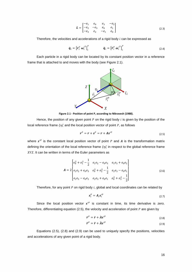
16

[

] (2.3)

Therefore, the velocities and accelerations of a rigid body can be expressed as

[

]

[

]

(2.4)

Each particle in a rigid body can be located by its constant position vector in a reference

frame that is attached to and moves with the body (see Figure 2.1).

Figure 2.1 - Position of point P, according to Nikravesh (1988).

Hence, the position of any given point on the rigid body is given by the position of the

local reference frame and the local position vector of point , as follows

(2.5)

where is the constant local position vector of point and is the transformation matrix

defining the orientation of the local reference frame in respect to the global reference frame

. It can be written in terms of the Euler parameters as

[

]

(2.6)

Therefore, for any point on rigid body , global and local coordinates can be related by

(2.7)

Since the local position vector is constant in time, its time derivative is zero.

Therefore, differentiating equation (2.5), the velocity and acceleration of point are given by

(2.8)

(2.9)

Equations (2.5), (2.8) and (2.9) can be used to uniquely specify the positions, velocities

and accelerations of any given point of a rigid body.

17

2.2 Kinematic Constraints

A kinematic constraint between two bodies imposes conditions on the relative

movement between them. Physically, they are imposed by joints, whose purpose is to transmit

motion between bodies in a certain way. If these constraints are expressed as algebraic

equations in terms of the generalized coordinates, they are called holomonic kinematic

constraints (Goldstein, 1980). A system of holomonic kinematic constraints can be

expressed as

( ) (2.10)

There can also be nonholomonic constraints, which are constraints that contain

inequalities or relations between velocity components. In the remainder of this text, the term

constraint will mean holomonic constraint unless otherwise specified.

Considering that is not known as an explicit function of time, it cannot be differentiated

to obtain or . Nevertheless, if the chain rule of differentiation is applied to equation (2.10)

with respect to time, the velocity constraint equation is obtained

( ) (2.11)

The application of the same method yields the acceleration constraint equation

( ) ( ) (2.12)

It’s usual to rewrite Eq. (2.12), in terms of the independent terms of the accelerations, as

( ) (2.13)

In a multibody system with no degrees of freedom and where is non-singular,

equations (2.10), (2.11) and (2.12) can be used to perform a kinematic analysis, determining ,

and for discrete time steps. In the following sections a brief description of the kinematic

joints necessary to develop the automobile models used in this dissertation is presented.

2.2.1 Spherical Joint

A spherical joint, more commonly known as ball joint, imposes that two bodies, and ,

share a common point (see Figure 2.2), which has constant coordinates with respect to each

body’s local reference frame.

Figure 2.2 - Spherical joint between two bodies.

18

The kinematic constraint equations can be expressed as

( )

(2.14)

restricting three degrees of freedom between the bodies, the three translations, allowing the

bodies to rotate freely with respect to one another.

2.2.2 Revolute Joint

A revolute joint only allows one relative rotation between bodies and . A point in the

axis of rotation of the revolute joint must have constant coordinates in the local reference frame

of both bodies. This constraint is similar to a spherical joint, and can be expressed through

equation (2.14). The remainder two rotations can be eliminated considering that vectors and

in Figure 2.3 must remain parallel to the joint axis at all times.

Figure 2.3 - Revolute joint between two bodies.

Therefore, the constraint equations for a revolute joint can be expressed as

( ) {

(2.15)

Note that in equation (2.15) the vector product between and yields three equations,

only two of which are linearly independent.

2.2.3 Cylindrical Joint

A cylindrical joint imposes that two bodies, i and j, share a common axis along which they

can slide and rotate relatively to one another. This can be achieved by stating that vectors

and must remain parallel to one another and to the joint axis at all times.

Figure 2.4 - Cylindrical joint between two bodies.

19

So, four constraint equations can be formulated for the cylindrical joint, yielding

( ) {

(

)

(2.16)

which restricts two translations and two rotations.

2.2.4 Translational Joint

A translational joint is very similar to a cylindrical joint where the relative rotation between

the bodies is constrained. Therefore, the cylindrical joint constraint equations are applicable,

with an added constraint stating that vectors and of Figure 2.5 must remain perpendicular

throughout the movement.

Figure 2.5 - Translational joint between two bodies.

Therefore, the five constraint equations for the translational joint are given by

( )

{

(

)

(2.17)

restricting two translations and three rotations.

2.3 Force Elements

Actuators, springs, dampers and the interaction between tires and the pavement are

examples of elements that exert external forces on a multibody system. Usually, these forces do

not act in the line of action of the center of mass, so an external force and an external

moment must be added to the force vector of the system.

2.3.1 Translational Springs

Two bodies, and , connected by a translational spring are shown in Figure 2.6. If is

the undeformed length, the deformed length and the stiffness, the force applied by the spring

is given by

( ) ( ) (2.18)

20

Figure 2.6 - Translational spring.

The translational spring applies forces to both bodies, acting on a common line, with

opposite directions to each other. The distance between the attachment points and is given

by

(2.19)

The magnitude of the deformed length is given by √ and the unit vector by .

The forces applied on bodies and , where ( ) is considered positive for ( ) and negative

for ( ), are given by

( ) ( ) (2.20)

( ) ( ) (2.21)

Note that the translational spring here presented is considered to be linear. However, the

spring may have nonlinear behavior and in that case Eq. (2.18) must be changed to

accommodate that behavior.

2.3.2 Translational Dampers

In a translational damper the damping force depends on the variation rate of the length .

Being the damping coefficient, the damping force can be calculated as

( ) (2.22)

The damper velocity is given by Eqs. (2.23) and (2.24).

(2.23)

(2.24)

Figure 2.7 - Translational damper.

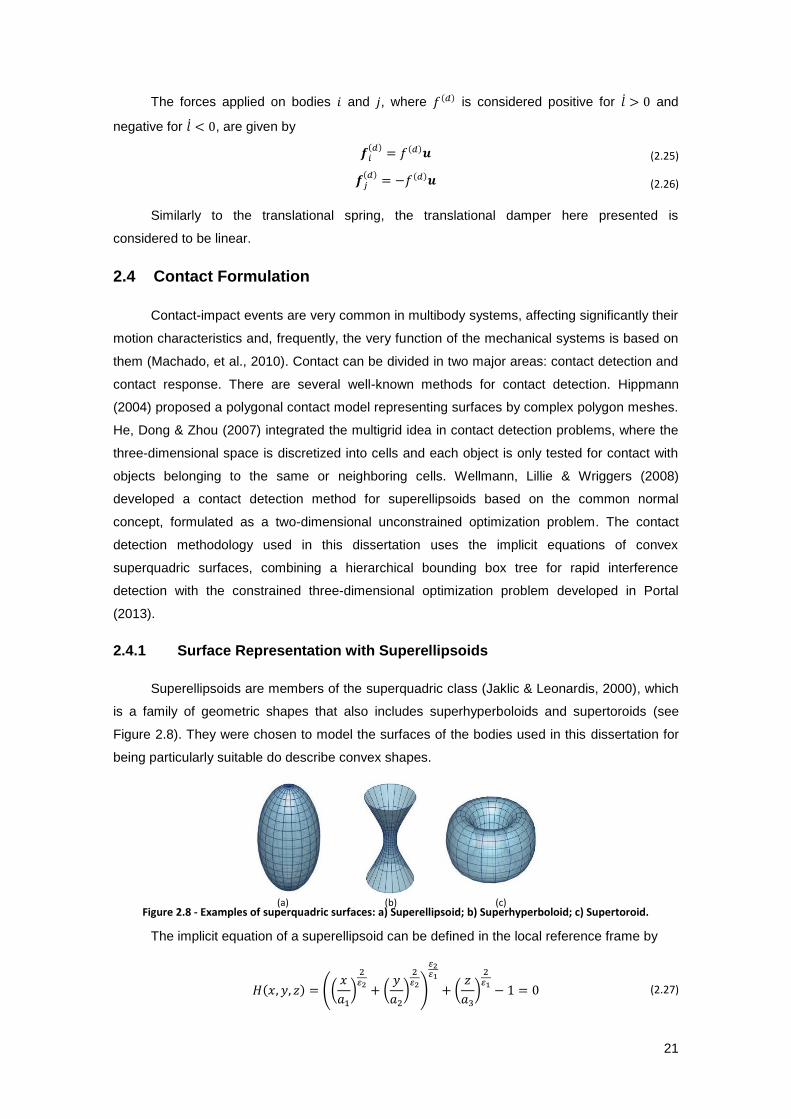
21

The forces applied on bodies and , where ( ) is considered positive for and

negative for , are given by

( ) ( ) (2.25)

( ) ( ) (2.26)

Similarly to the translational spring, the translational damper here presented is

considered to be linear.

2.4 Contact Formulation

Contact-impact events are very common in multibody systems, affecting significantly their

motion characteristics and, frequently, the very function of the mechanical systems is based on

them (Machado, et al., 2010). Contact can be divided in two major areas: contact detection and

contact response. There are several well-known methods for contact detection. Hippmann

(2004) proposed a polygonal contact model representing surfaces by complex polygon meshes.

He, Dong & Zhou (2007) integrated the multigrid idea in contact detection problems, where the

three-dimensional space is discretized into cells and each object is only tested for contact with

objects belonging to the same or neighboring cells. Wellmann, Lillie & Wriggers (2008)

developed a contact detection method for superellipsoids based on the common normal

concept, formulated as a two-dimensional unconstrained optimization problem. The contact

detection methodology used in this dissertation uses the implicit equations of convex

superquadric surfaces, combining a hierarchical bounding box tree for rapid interference

detection with the constrained three-dimensional optimization problem developed in Portal

(2013).

2.4.1 Surface Representation with Superellipsoids

Superellipsoids are members of the superquadric class (Jaklic & Leonardis, 2000), which

is a family of geometric shapes that also includes superhyperboloids and supertoroids (see

Figure 2.8). They were chosen to model the surfaces of the bodies used in this dissertation for

being particularly suitable do describe convex shapes.

Figure 2.8 - Examples of superquadric surfaces: a) Superellipsoid; b) Superhyperboloid; c) Supertoroid.

The implicit equation of a superellipsoid can be defined in the local reference frame by

( ) ((

)

(

)

)

(

)

(2.27)

(a) (b) (c)

22

where , and represent the semi-axes and and are the exponents that define the

shape. Varying the value of these exponents, the superellipsoid can assume several shapes, as

depicted in Figure 2.9.

Figure 2.9 – Influence of shape exponents in a superellipsoid with semi-axes and semi-axis .

The normal vector to the surface of a superellipsoid is given by the gradient of its

implicit equation, as expressed in Eq. (2.28)

( ) ( ) [

]

[ ] (2.28)

where the components are given by

[(

)

(

)

]

(

)

(2.29)

[(

)

(

)

]

(

)

(2.30)

(

)

(2.31)

The formulas presented in Eq. (2.27) and in Eqs. (2.29) to (2.31) are written in the local

reference frame of the superellipsoid. Their representation in the global reference frame is

achieved with the application of coordinate transformations. The translation is given by the

vector [ ] , representing the position vector of the geometric center of the ellipsoid.

The transformation matrix, here denoted as , is given by Eq. (2.6). The implicit superellipsoid

equation can now be rewritten in the global reference frame as

( ) (( ) ( )

)

( )

(2.32)

where the terms are defined as

( ) ( ) ( )

(2.33)

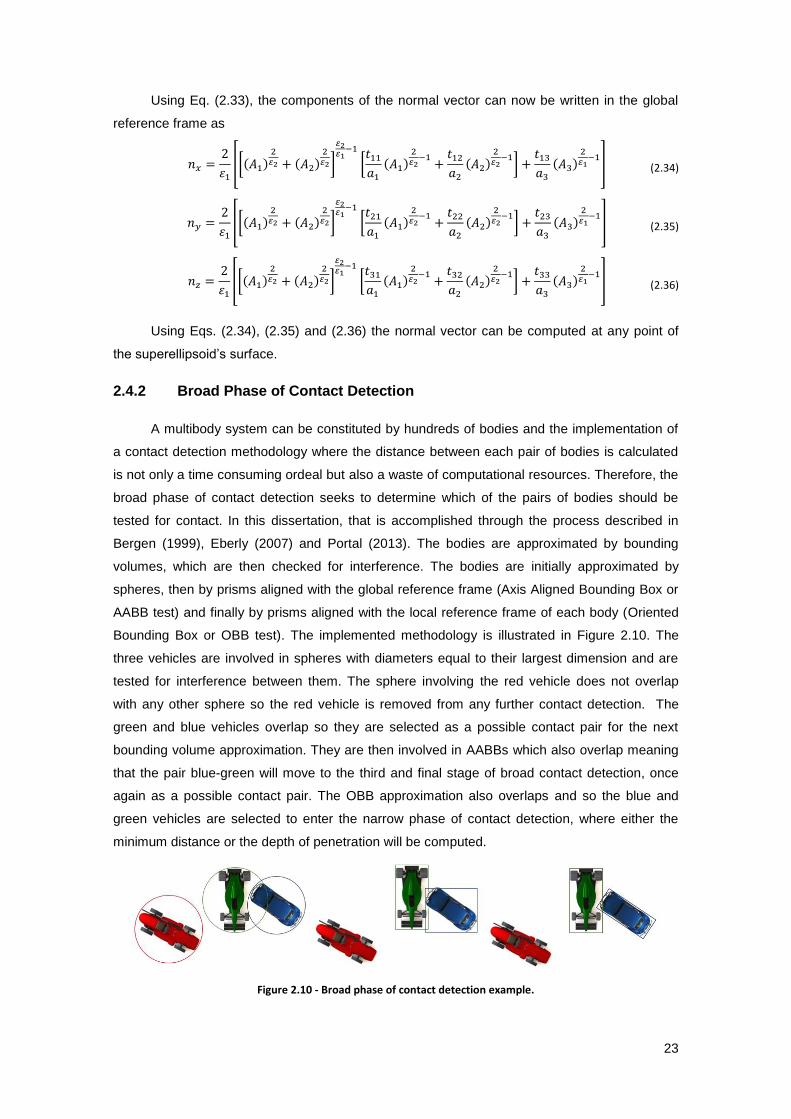
23

Using Eq. (2.33), the components of the normal vector can now be written in the global

reference frame as

[[( )

( )

]

[ ( )

( )

]

( )

] (2.34)

[[( )

( )

]

[ ( )

( )

]

( )

] (2.35)

[[( )

( )

]

[ ( )

( )

]

( )

] (2.36)

Using Eqs. (2.34), (2.35) and (2.36) the normal vector can be computed at any point of

the superellipsoid’s surface.

2.4.2 Broad Phase of Contact Detection

A multibody system can be constituted by hundreds of bodies and the implementation of

a contact detection methodology where the distance between each pair of bodies is calculated

is not only a time consuming ordeal but also a waste of computational resources. Therefore, the

broad phase of contact detection seeks to determine which of the pairs of bodies should be

tested for contact. In this dissertation, that is accomplished through the process described in

Bergen (1999), Eberly (2007) and Portal (2013). The bodies are approximated by bounding

volumes, which are then checked for interference. The bodies are initially approximated by

spheres, then by prisms aligned with the global reference frame (Axis Aligned Bounding Box or

AABB test) and finally by prisms aligned with the local reference frame of each body (Oriented

Bounding Box or OBB test). The implemented methodology is illustrated in Figure 2.10. The

three vehicles are involved in spheres with diameters equal to their largest dimension and are

tested for interference between them. The sphere involving the red vehicle does not overlap

with any other sphere so the red vehicle is removed from any further contact detection. The

green and blue vehicles overlap so they are selected as a possible contact pair for the next

bounding volume approximation. They are then involved in AABBs which also overlap meaning

that the pair blue-green will move to the third and final stage of broad contact detection, once

again as a possible contact pair. The OBB approximation also overlaps and so the blue and

green vehicles are selected to enter the narrow phase of contact detection, where either the

minimum distance or the depth of penetration will be computed.

Figure 2.10 - Broad phase of contact detection example.

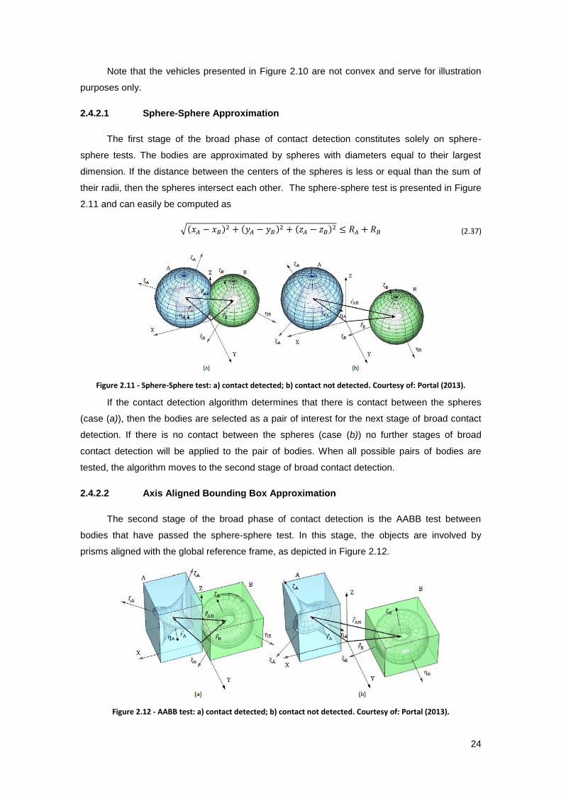
24

Note that the vehicles presented in Figure 2.10 are not convex and serve for illustration

purposes only.

2.4.2.1 Sphere-Sphere Approximation

The first stage of the broad phase of contact detection constitutes solely on sphere-

sphere tests. The bodies are approximated by spheres with diameters equal to their largest

dimension. If the distance between the centers of the spheres is less or equal than the sum of

their radii, then the spheres intersect each other. The sphere-sphere test is presented in Figure

2.11 and can easily be computed as

√( ) ( )

( ) (2.37)

Figure 2.11 - Sphere-Sphere test: a) contact detected; b) contact not detected. Courtesy of: Portal (2013).

If the contact detection algorithm determines that there is contact between the spheres

(case (a)), then the bodies are selected as a pair of interest for the next stage of broad contact

detection. If there is no contact between the spheres (case (b)) no further stages of broad

contact detection will be applied to the pair of bodies. When all possible pairs of bodies are

tested, the algorithm moves to the second stage of broad contact detection.

2.4.2.2 Axis Aligned Bounding Box Approximation

The second stage of the broad phase of contact detection is the AABB test between

bodies that have passed the sphere-sphere test. In this stage, the objects are involved by

prisms aligned with the global reference frame, as depicted in Figure 2.12.

Figure 2.12 - AABB test: a) contact detected; b) contact not detected. Courtesy of: Portal (2013).

25

Before detailing the test, it’s useful to introduce the concept of separating axis. An

arbitrary vector is a separating axis if an only if the projections of the objects onto do not

overlap. For non-intersecting convex objects, a separating axis always exists (Bergen, 2004).

This property is illustrated in Figure 2.13 where it is clear that, as the projections of the vehicles

do not overlap on , then is a separating axis and the vehicles are not in contact.

Figure 2.13 - Separating axis test between two vehicles.

Considering the two AABBs shown in Figure 2.14, their projections on an arbitrary vector

are given by

| | | | | | (2.38)

| | | | | | (2.39)

where ( ) and ( ) are the dimensions of the boxes obtained from the

maximum dimensions of the bodies. For the bodies not to be in contact, must be a separating

axis, meaning that

| | (2.40)

Figure 2.14 - Separating axis test (SAT) between two AABBs. Courtesy of: Portal (2013).

Since the bounding volumes are aligned with the global reference frame, the axes that

might separate them are the global X, Y and Z axes. Therefore, the separating axis test is

executed three times, at most, for each pair of bodies. If none of the tests is satisfied, the bodies

are in contact and proceed as a pair of interest to the third and final stage of broad contact

detection. If one separating axis is found, the objects are not in contact.

26

The quantities that must be determined for the SAT test are summarized in Table 2.1.

Table 2.1 - SAT test quantities for the AABB test.

Axis Projection Projection | |

| | |

| | | |

| | | |

| | |

| | |

| | | |

| | | |

| | |

| | |

| | | |

| | | |

| | |

Note that the terms refer to the transformation matrix of each body (Eq. (2.6)).

2.4.2.3 Oriented Bounding Box Approximation

The third and final stage of the broad phase of contact detection is very similar to the

second stage, the difference being that the bounding volumes are now aligned with the local

reference frame of each body, as it can be seen in Figure 2.15.

Figure 2.15 - OBB test: a) contact detected; b) contact not detected. Courtesy of: Portal (2013).

As the bounding volumes are now oriented, instead of three there are fifteen axis that

need to be tested for overlapping. Six of those axes correspond to the axes of the local

reference frame of both bodies and the remainder nine to the cross products between them.

The necessary quantities to perform the OBB test are summarized in Table 2.2, where

represent the components of the matrix product between the transformation matrices of both

bodies.

[

] (2.41)

27

Table 2.2- SAT test quantities for OBB test.

Axis Projection Projection | |

| | |

| | | | |

| | |

| | | | |

| | |

| | | | |

| | |

| | | |

|

| | |

| | | |

|

| | |

| | | |

|

| | |

| | | |

| |

|

| | |

| | | |

| |

|

| | |

| | | |

| |

|

| | |

| | | |

| |

|

| | |

| | | |

| |

|

| | |

| | | |

| |

|

| | |

| | | |

| |

|

| | |

| | | |

| |

|

| | |

| | | |

| |

|

If no separating axis is found, then the OBB are in contact and the pair of bodies is

selected to enter the narrow phase of contact detection.

2.4.3 Narrow Phase of Contact Detection

The methodology used in the narrow phase is the one presented by Portal, Dias & Sousa

(2009), developed in Portal (2013) for contact detection between convex superquadric surfaces.

Contact detection is treated as a nonlinear optimization problem that minimizes the

squared distance between two surfaces, A and B (see Figure 2.16), subject to three equality

constraints. The first two constraints are the implicit equations of the superellipsoids (Eq.

(2.32)), ensuring that the optimal solution is located over the surfaces. These constraints

however, are not enough to guarantee convergence to the intended minimum distance. For

instance, in a case where penetration exists, the optimization problem would converge to a null

distance and not to the intended maximum interference. Therefore, a third constraint is

necessary, given in this case by an alignment condition (Pombo & Ambrósio, 2007). The third

constraint states that at the optimal solution the normal vectors to the surfaces must be

collinear, corresponding the penetration to the maximum elastic deformation.

28

Figure 2.16 - Design variables and objective function for the optimization problem. Courtesy of: Portal (2013).

The formulation of the optimization problem is presented in Eqs. (2.42) to (2.45). Note

that the formulation presented is the one that achieved better results and information about

alternative sets of constraints can be found in Portal, Dias & Sousa (2010).

( ) ‖ ‖

‖

‖ (2.42)

(

) (2.43)

(

) (2.44)

(2.45)

When the optimization algorithm converges to a minimum distance value

, a contact

condition must be calculated in order to determine if this value corresponds to a maximum

penetration or to a minimum distance between the surfaces.

Maximum Penetration

(2.46)

Minimum Distance

The optimization routine to solve the narrow phase of contact detection problem was not

implemented by the author in the course of the present dissertation but provided by Dr. Portal in

a Fortran dll and in a Matlab m-file which were integrated in the multibody dynamics code.

2.5 Normal Contact-Impact Force Models

When bodies come into contact, the compression phase begins. The bodies deform

along the normal direction to the contact surface, while the relative velocity in that direction is

progressively reduced to zero. When the relative normal velocity reaches zero, the instant of

maximum penetration is achieved, the compression phase ends and the restitution phase

begins. The relative normal velocity starts increasing and, when the bodies are again separated

from one another, the restitution phase ceases (Brach, 1991). Contact can also affect tangential

sliding by means of frictional forces that act through part or all of the contact duration. Due to its

simplicity and ability to characterize the contact phenomenon, the contact forces are modelled

with a continuous force model. Contact-impact modelling is one of the most interesting subjects

29

in multibody dynamics and still is an active field of research (Najafabadi, Kovecses, & Angeles,

2008).

2.5.1 Nonlinear Elastic Hertz Model

Hertz (1896) developed a nonlinear contact force model, relating the contact force with a

nonlinear parameter of penetration that is only valid for elastic materials. The normal contact

force can be expressed as

(2.47)

where is a generalized stiffness parameter, represents the penetration between the bodies

and is a nonlinear parameter of penetration. The characteristic behavior of colliding bodies

modelled by the nonlinear elastic Hertz model is presented in Figure 2.17.

Figure 2.17 - Nonlinear elastic Hertz model behavior: (a) normal contact force versus penetration; (b) normal contact force and penetration versus time.

Hertz’s model became the basis for several following models, in which several authors

added dissipative terms to account for energy loss. These models became known as Hertzian

models.

2.5.2 Nonlinear Dissipative Lankarani and Nikravesh Model

Lankarani & Nikravesh (1990) and Lankarani & Nikravesh (1994) developed a continuous

force model that conjugates Hertz’s law with a hysteresis damping factor, by means of a

nonlinear parameter. The normal contact force is given by

(2.48)

where is a damping coefficient and is the relative normal contact velocity. The damping

factor relates kinetic energy loss in the colliding bodies with energetic loss due to internal

damping. The damping coefficient assumes the form given by

(2.49)

with

( )

( ) (2.50)

30

where represents the hysteresis damping factor, is the generalized stiffness

parameter, stands for the coefficient of restitution and ( ) represents the initial penetration

velocity. This formulation can be understood as if the contact regions of the colliding bodies are

covered with spring damper elements. The nonlinear dissipative model is then obtained with the

substitution of the damping factor into Eq. (2.48), and can be expressed as

[ ( )

( )] (2.51)

The characteristic behavior of colliding bodies modelled by the Lankarani and Nikravesh

model is presented in Figure 2.18.

Figure 2.18 - Nonlinear dissipative Lankarani and Nikravesh model behavior: (a) normal contact force versus penetration; (b) normal contact force and penetration versus time.

The authors of this model state that it’s only valid for small energy losses, i.e., for

coefficients of restitution close to unity. This is not the case of a road traffic accident, where the

values for the coefficient of restitution generally lie in the range between 0 and 0.3. It can be

seen that the larger the vehicle deformations, the lower the coefficient of restitution. Only for

very low velocity impacts are values higher than 0.3 realistic (Siegmund, King, & Montgomery,

1996).

Note that the Kelvin-Voigt model (Goldsmith, 1960) was the first to introduce a dissipative

term to model energetic loss during contact and that the Hunt & Crossley (1975) model was

the first to introduce a nonlinear term to the damping coefficient . The Lankarani and

Nikravesh model is an extent of their work.

2.5.3 Nonlinear Dissipative Flores et al. Model

Flores et al. (2011) and Machado et al. (2012) refined the Lankarani and Nikravesh

model making it able to describe soft materials, establishing a relation between the hysteresis

damping factor and the coefficient of restitution. The hysteresis damping factor is expressed as

( )

( ) (2.52)

being the contact force given by

31

[

( )

( )] (2.53)

The characteristic behavior of the colliding bodies modeled by the Flores et al. model is

presented in Figure 2.19.

Figure 2.19 - Nonlinear dissipative Flores et al. model behavior: (a) normal contact force versus penetration; (b) normal contact force and penetration versus time.

The Flores et al. (2011) contact force model is the one implemented in the multibody

dynamics code developed in this dissertation. Note that one of the drawbacks of this method is

the difficulty to choose contact parameters such as the equivalent stiffness or the degree of

nonlinearity of the penetration. Also, in conjunction with the contact detection methodology,

contact is modelled as a local phenomenon, being valid for small deformations. In a road traffic

accident this is often not the case as the deformations are usually large. This is one of the

simplifying hypotheses of the developed model.

2.6 Tangential Contact-Impact Force Models

Coulomb’s law of dry friction states that when two bodies slide against each other, a

friction force directly proportional to the normal contact force and independent of the contact

area, acts in the opposite direction of the relative velocity. Friction is, however, a much more

complex phenomenon, in which different modes can occur, such as sticking or sliding. Sticking,

for instance, occurs when the relative tangential velocity of the bodies begins to approach zero,

depending on a parameter that is not taken into account by Coulomb’s law. Thus, a continuous

friction force model which considers the relative tangential velocity is required (Flores,

Ambrósio, Claro, & Lankarani, 2008). The computational implementation of Coulomb’s friction

law leads to numerical difficulties due to the discontinuity when the relative tangential velocity

is null. To overcome this, Threlfall (1978) proposed a friction force model with a smooth

transition from to given by

‖ ‖

[ ‖ ‖ ] (2.54)

for | | ‖ ‖. In Eq. (2.54) is the coefficient of friction, is the normal contact force and

represents a small velocity parameter.

32

Ambrósio (2003) proposed an alternative method of smoothing Coulomb’s friction law

that uses a dynamic friction force given by

‖ ‖

(2.55)

where is a dynamic correction coefficient expressed by

{

‖ ‖

‖ ‖ ‖ ‖ ‖ ‖

(2.56)

with tolerances and for the tangential velocity. The dynamic correction coefficient allows

the numerical stabilization of the integration algorithm by preventing changes in the direction of

the friction force for almost null values of tangential velocity. Figure 2.20 presents a comparison

between both friction force models.

Figure 2.20 - Friction force models: Left - Threlfall (1978); Right - Ambrósio (2003).

The model proposed by Ambrósio (2003) is the friction force model implemented in the

multibody dynamics code developed in the present dissertation.

2.7 Tire Model

The main function of an automotive tire is to transmit forces and moments for vehicle

steering control. It transmits the forces that drive, brake and guide the vehicle. Since the tire

forces control the vehicle motion predicted by a simulation, the tire model is a critical feature for

its accuracy. This is particularly true in traffic accident reconstructions where each wheel can be

subjected to a wide range of dynamic conditions. The important role that tires play in the

performance of a vehicle has made their behavior the subject of continuous studies for the past

eighty years, resulting on a large number of known tire models. Some use simple linear or

nonlinear models with coefficients obtained by experimental data and curve fitting, being the

most known the Magic Formula (Pacejka & Sharp, 1991). Others were developed through finite

element models such as Mousseau & Hulbert (1996) or Musseau, Darnell & Hulbert (1997).

Simpler but still accurate tire models are also available, such as the BNP tire model (Bakker,

Nyborg, & Pacejka, 1987), the NCB tire model (Brach & Brach, 2000) or the TMeasy tire model

(Hirschberg, Rill, & Weinfurter, 2007).

33

The tire model implemented in this dissertation is the one proposed by Gim & Nikravesh

(1990), known as the University of Arizona (UA) Tire Model. Figure 2.21 shows the SAE J670

reference frame, where several variables are illustrated. The reference frame has its origin at

the intersection of the z axis with the road plane, the x axis corresponds to the intersection of

the wheel plane with the road plane and the y axis is the cross product between x and z. The

camber angle, , is defined by the angle between the wheel plane and the XY plane. The slip

angle, , is the angle between the tire’s heading and traveling direction, computed as

( ⁄ ).

Figure 2.21 – SAE J670 reference tire frame. Courtesy of: Portal (2013).

Slip occurs at all times during vehicle motion, being the slip ratio, , a measure of the

wheel slip at the contact region with the ground. To calculate , it’s assumed that the center of

the tire is motionless and that the ground is moving with a relative velocity to the tire .

The velocity of the tire at the contact point with the ground will then be , where is

the effective radius of the tire (Figure 2.22). Considering that with a non-zero slip angle the

longitudinal velocity is , the slip velocity can then be expressed as

√( ) ( )

and the longitudinal slip ratio can be defined as

[

(2.57)

representing two opposite situations, i.e., braking and driving, respectively.

2.7.1 University of Arizona Tire Model

The UA tire model (Gim & Nikravesh, 1990) approximates the tire by an undeformable

torus shape, which is then used to calculate the deformation analytically. The deformation is

defined by the penetration of the tire on the ground (Figure 2.22), being the normal force, ,

calculated using a spring-damper model.

34

(2.58)

where is the radial stiffness and the damping coefficient. The longitudinal force is a

function of the normal force, the longitudinal stiffness and the longitudinal friction

coefficient . The lateral forces are a function of the lateral stiffness , the normal force, the

slip angle, the camber angle and the lateral friction coefficient . According to Coulomb’s

theory of rigid body friction, the coefficient of sliding friction is independent of direction and load,

i.e. . However, experimental data has shown that for tires, differences between

these values do occur (Warner, Smith, James, & Germane, 1983). In this dissertation the values

of coefficients of friction are considered to be the same. The forces generated by the road on

the tires are presented next

Longitudinal Force

Lateral Forces

Self-Alignment Torque Rolling Resistance Torque

[

(

)

[

(

)

[

[ [(

)

]

(2.59)

(2.60)

(2.61)

(2.62)

(2.63)

where is the deflection velocity, and

are the components of the lateral force, respectively

due the sideslip and the camber angles, ⁄ is the instantaneous slip ratio where

represents the critical slip ratio, is the critical slip ratio due to the slip angle and

is the limit

slip ratio due to the camber angle.

Figure 2.22 - Geometric characteristics of the UA tire model. Courtesy of: Portal (2013).

The UA tire model can be applied to horizontal and non-horizontal terrain, being the

penetration computed in the normal direction to the ground. In the present dissertation,

however, the ground is assumed to be horizontal.

35

2.8 Equations of Motion for Unconstrained Multibody Systems

Considering as the sum of all forces acting on body i and the sum of all moments

around its center of mass, the Newton-Euler equations of motion can be written as

(2.64)

where is the vector of angular velocities,

the vector of angular accelerations, the inertia

tensor and

the Coriolis forces. If the origin of the local reference frame is set to coincide

with the center of mass, the mass matrix of body i is given by

[

] (2.65)

where is the identity matrix. Moreover, if the local reference frame is aligned with the principal

axes of inertia, the products of inertia are null, resulting in a diagonal inertia tensor.

[

] (2.66)

Consequently, the equations of motion of body i can be written as

(2.67)

where the term is the generalized force vector, given by

[

] (2.68)

For a system of unconstrained bodies, equation (2.67) can be generalized to consider

all bodies that constitute the system, yielding

(2.69)

where

[

] [

] [

] (2.70)

Note that even though the equations are written in terms of all bodies that constitute the

system, they are not coupled.

2.9 Equations of Motion for Constrained Multibody Systems

If two or more bodies are connected by a joint, then the multibody system is said to be

constrained. A kinematic constraint imposes restrictions on the relative movement between the

bodies by means of reaction forces. Therefore, equation (2.69) has to be rewritten in order to

encompass an additional term representing the joint reaction forces, , as

36

(2.71)

The joint reaction forces generated by the kinematic constraints are calculated using the

jacobian of kinematic constraints and a vector of Lagrange multipliers (Haug, 1989), as

(2.72)

Substituting Eq. (2.72) in Eq. (2.71) yields

(2.73)

which, in conjunction with Eqs. (2.10), (2.11) and (2.12) comprise the complete set of equations

of motion for a constrained multibody system.

Appending the equation of acceleration kinematic constraints, Eq. (2.12), into Eq. (2.73),

a system of differential equations and algebraic equations is obtained and can be solved

through numerical methods.

[

] [ ] [

] (2.74)

This is a second order mixed system of differential and algebraic equations. Except for

very simple problems, an exact closed solution cannot be found. Furthermore, its numerical

solution is not trivial since it requires special integration methods capable of dealing with this

kind of system of equations and of providing a stable and accurate integration. The numerical

integration of the equations of motion can be done by means of direct integration of the

differential algebraic equations or by transforming them into a system of first order ordinary

differential equations (Ascher, Chin, Petzold, & Reich, 1995). For solving differential algebraic

equations, the backward difference formulae (Yen & Petzold, 1998) or implicit Runge-Kutta

methods (Potra, 1995) can be used. However, when compared to ordinary differential equations

integrators, they present slower integration speed, require iterative processes for the solution

and result in a more complex set of nonlinear algebraic equations. For an outline of several

integration methods, see the work by Gear & Petzold (1984).

2.10 Solution of the Equations of Motion

The differential equation given by Eq. (2.12) is unstable and during the course of the

integration numerical errors will increase with time. They are caused by the approximate

solutions obtained for velocities and accelerations (Chang & Nikravesh, 1985) and, even though

they are small and can be neglected in the first time steps of the analysis (Flores, Ambrósio,

Claro, & Lankarani, 2008), their increase in time will lead to constraint violations, requiring some

type of stabilization method to be introduced in the system (Neto & Ambrósio, 2003).

Several methods were proposed to address this issue. In the coordinate partitioning

method (Wehage & Haug, 1982) the separation of positions and velocities into dependent and

independent coordinates avoids constraint violations. This method, however, has a high

computational cost, derived from the necessity of an iterative solution to calculate the positions

37

and the instability created by changing the number of independent coordinates during the

analysis. The Augmented Lagrangean Formulation (Bayo & Ledesma, 1996) guarantees minor

constraint violations and is capable of dealing with singular configurations and redundant

kinematic constraints. Formulations based in velocity transformations such as the ones

proposed by Kim & Vanderploeg (1986) or Nikravesh (1990) can also be used. These are

efficient but complex to implement and have a large computational cost due to the several

produces of matrices needed to form the system of equations. Finally, there is a constraint

stabilization scheme, derived from feedback control theory, which solves the system presented

in Eq. (2.74) with an added constraint stabilization (Baumgarte, 1972). As it’s often the case in

feedback control of dynamic systems, the constraints are allowed to be slightly violated before

corrective actions arise in order to force the violation to fade, doing so by feeding back the

position and velocity of constraint violations to dampen the acceleration of constraint violations.

The Baumgarte (1972) constraint violation stabilization method replaces the acceleration

constraint equation, Eq. (2.12), by

(2.75)

where and are positive feedback control parameters for the velocity and position constraint

violations, respectively, resulting on the system presented on Eq. (2.76). The proper choice of

feedback parameters is not straightforward and is dependent on the numerical integrator used

and the value of the time step (Chang & Nikravesh, 1985). The use of values between 1 and 10

are suggested, as well as the use of , in order to obtain a critical damping in the oscillation

of the response. For a multibody system comprised of rigid bodies, Baumgarte pointed out that

results well for the integration method.

[

] [ ] [

] (2.76)

The added term doesn’t solve all the instabilities or singular configurations (Haug, 1989),

but provides an efficient method for the integration of the equations of motion with constraint

violation stabilization, has a small computational cost and is simple and efficient when

compared to the other methods. Nikravesh (1984) performed a comparative study between the

direct integration of the equations of motion, the coordinate partitioning method and the

Baumgarte constraint stabilization method, having concluded that the Baumgarte approach is

the most efficient of the three. The Baumgarte constraints violation stabilization method is the

one used in the present dissertation. The adopted values for the feedback parameters are

. For a parametric study of the effects of the feedback parameters see Flores,

Machado, Seabra & Silva (2011).

The solution of the initial value problem implies that initial conditions regarding positions

and velocities must be given, in order to guarantee the uniqueness of the solution. Moreover,

Gear (1971) showed that the initial conditions must satisfy the position and velocity constraints

of Eqs. (2.10) and (2.11). The system of equations of motion presented in Eq. (2.76) is solved

by a Gauss-Jordan elimination method (Chapra & Canale, 2009) to obtain the acceleration

38

vector, , and the Lagrange multipliers . Then, the system of second order differential

equations is converted in a system of first order differential equations (Shampine & Gordon,

1975), trough the definition of two vectors, and , with the positions and velocities and the

velocities and accelerations, respectively

[ ] [

] (2.77)

Then, in each integration time step, the accelerations vector, , together with the

velocities vector, , are integrated in order to obtain the system’s velocities and positions for the

next time step, being this procedure repeated until the final instant of the analysis is reached.

( ) → ( ) (2.78)

Note that when the gross motion of the overall multibody system is combined with the

sudden appearance of non-linear contact forces, rapid changes in accelerations and velocities

arise, thus inducing a stiff behavior in the system. Bearing this in mind, the integration algorithm

implemented is the one proposed in Gear (1981) and Gear & Petzold (1984).

Arguably, the most complex part of the implementation of a multibody dynamics code is

to establish an accurate procedure to deal with the contact-impact phase. In general, contact is

a fleeting phenomenon, being the proper selection of the integration time step mandatory in

order to achieve accurate results. A conservative approach would be to use very small time

steps throughout the analysis. This solution, however, is not computationally efficient, since

small time steps are only required when the dynamics of the system is characterized by high

frequencies, translated in this case by high force levels, short duration, large changes in the

velocities of the bodies and rapid energy dissipation from one time instant to the next (Gilardi &

Sharf, 2002). If this is not the case, larger integration time steps may and should be used. Using

a high time step when contact is detected, the depth of penetration between the colliding bodies

will most likely be artificially high, leading to a contact force with no real physical meaning,

which, in turn, may lead to post-impact dynamics unrelated to the physical problem due to the

gain of energy induced by the abnormally high contact force value. Therefore, the algorithm

implemented in the present dissertation has the ability to, when contact is detected, trace back

to the previous time instant and adjust the time step, insuring a smooth transition between non-

contact and contact situations and that, in the vicinity of contact, the penetration is bellow a

prescribed threshold. This was done through the implementation of procedure 1 described in

Flores & Ambrósio (2010). The implemented methodology for the solution of the equations of

motion is schematized in Figure 2.23.

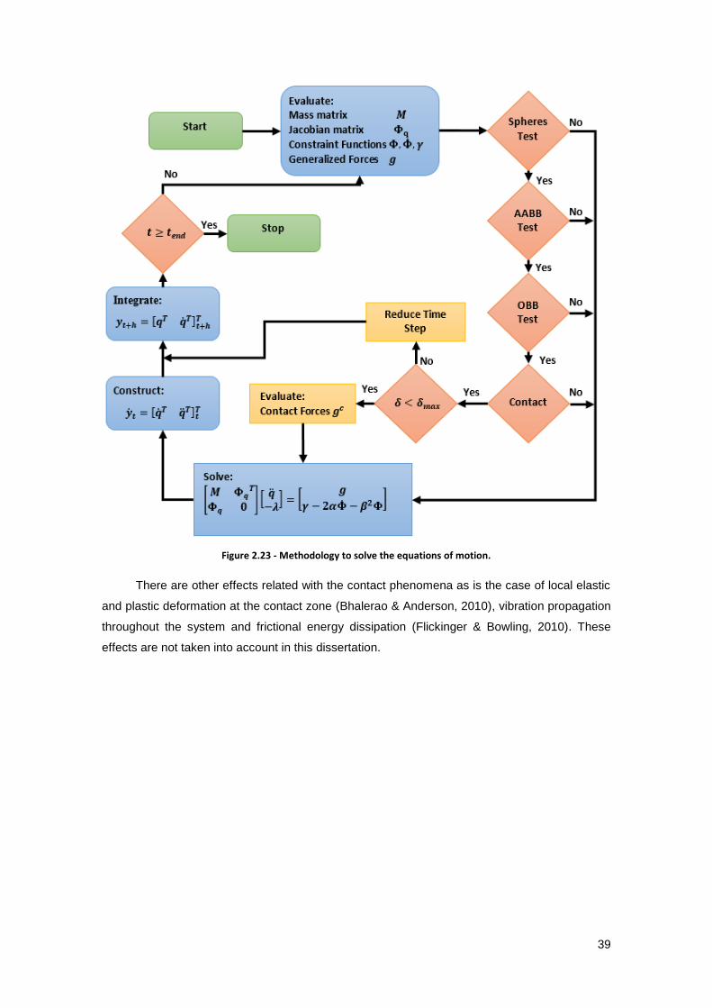
39

Figure 2.23 - Methodology to solve the equations of motion.

There are other effects related with the contact phenomena as is the case of local elastic

and plastic deformation at the contact zone (Bhalerao & Anderson, 2010), vibration propagation

throughout the system and frictional energy dissipation (Flickinger & Bowling, 2010). These

effects are not taken into account in this dissertation.

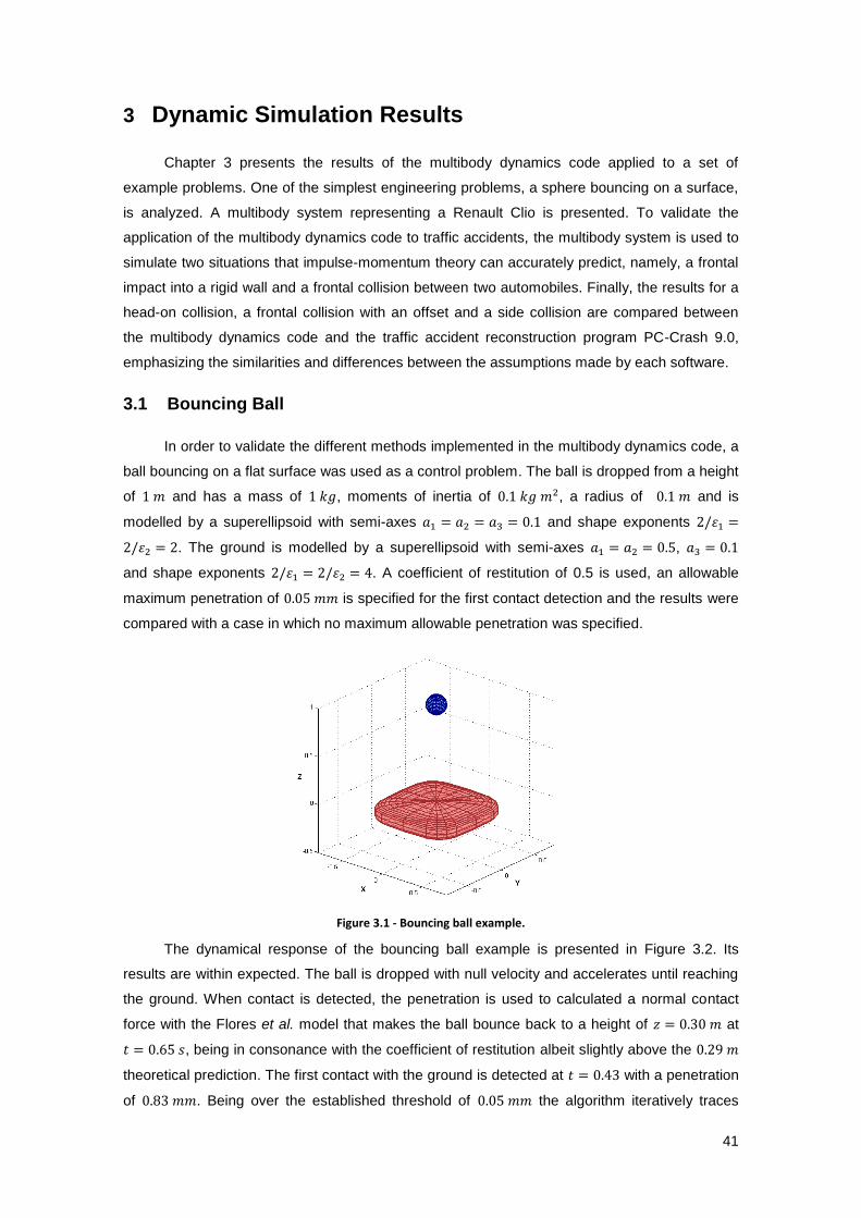
41

3 Dynamic Simulation Results

Chapter 3 presents the results of the multibody dynamics code applied to a set of

example problems. One of the simplest engineering problems, a sphere bouncing on a surface,

is analyzed. A multibody system representing a Renault Clio is presented. To validate the

application of the multibody dynamics code to traffic accidents, the multibody system is used to

simulate two situations that impulse-momentum theory can accurately predict, namely, a frontal

impact into a rigid wall and a frontal collision between two automobiles. Finally, the results for a

head-on collision, a frontal collision with an offset and a side collision are compared between

the multibody dynamics code and the traffic accident reconstruction program PC-Crash 9.0,

emphasizing the similarities and differences between the assumptions made by each software.

3.1 Bouncing Ball

In order to validate the different methods implemented in the multibody dynamics code, a

ball bouncing on a flat surface was used as a control problem. The ball is dropped from a height

of and has a mass of , moments of inertia of , a radius of and is

modelled by a superellipsoid with semi-axes and shape exponents

. The ground is modelled by a superellipsoid with semi-axes ,

and shape exponents . A coefficient of restitution of 0.5 is used, an allowable

maximum penetration of is specified for the first contact detection and the results were

compared with a case in which no maximum allowable penetration was specified.

Figure 3.1 - Bouncing ball example.

The dynamical response of the bouncing ball example is presented in Figure 3.2. Its

results are within expected. The ball is dropped with null velocity and accelerates until reaching

the ground. When contact is detected, the penetration is used to calculated a normal contact

force with the Flores et al. model that makes the ball bounce back to a height of at

, being in consonance with the coefficient of restitution albeit slightly above the

theoretical prediction. The first contact with the ground is detected at with a penetration

of . Being over the established threshold of the algorithm iteratively traces

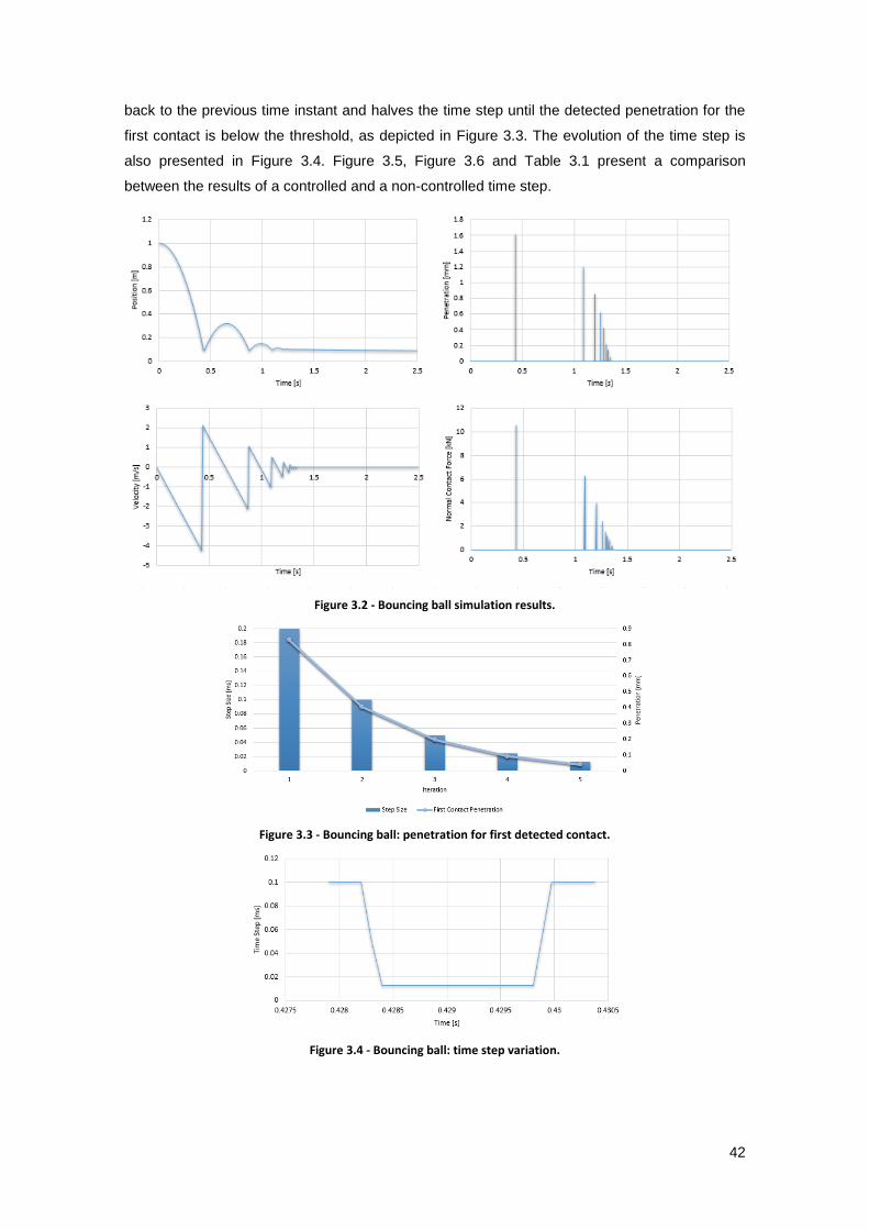
42

back to the previous time instant and halves the time step until the detected penetration for the

first contact is below the threshold, as depicted in Figure 3.3. The evolution of the time step is

also presented in Figure 3.4. Figure 3.5, Figure 3.6 and Table 3.1 present a comparison

between the results of a controlled and a non-controlled time step.

Figure 3.2 - Bouncing ball simulation results.

Figure 3.3 - Bouncing ball: penetration for first detected contact.

Figure 3.4 - Bouncing ball: time step variation.

43

Figure 3.5 - Bouncing ball: comparison of normal contact force and penetration during the first contact period between the non-controlled and the controlled cases.

Figure 3.6 - Bouncing ball: comparison of velocities during the first contact period between the non-controlled and the controlled cases.

Table 3.1 - Comparison of pre and post impact states between the controlled and the non-controlled case.

Case Pre-Contact Velocity

[m/s] Post-Contact Velocity

[m/s] Coefficient of

Restitution

Controlled -4.20 2.23 0.53

Non-Controlled -3.99 2.79 0.70

When compared to a case in which the allowable maximum penetration for the first

contact is not controlled, it’s clear that this method is crucial for the accuracy of results.

Controlling the time step according to an allowable value for the first penetration leads to an

overall smaller contact force and a longer period of contact, leading to a far more accurate post

impact dynamics (Figure 3.6 and Table 3.1)

3.2 Multibody Model of an Automobile

The multibody model implemented in this dissertation is based on the one developed in

Portal (2006). The representative model is presented in Figure 3.7 and is comprised of nine

rigid bodies and eight kinematic joints, having eighteen degrees of freedom. The model was set

to mimic a Renault Clio, arguably the most common vehicle in Portugal, in terms of dynamic

properties. Its main characteristics are presented in Table 3.2 and detailed information of the

multibody system is presented from Table 3.3 to Table 3.6.

44

Figure 3.7 - Multibody model of an automobile.

Table 3.2 - Characteristics of the vehicle.

Property Value

Total Mass 980 kg

Length 3.775 m

Width 1.640 m

Height 1.420 m

Wheelbase 2.470 m

Track Width 1.405 m

Table 3.3 - Geometrical and inertial properties of the elements of the multibody system.

Body Superellipsoid

semi-axes and [m]

Superellipsoid shape parameters

( ⁄ ) and ( ⁄ )

Mass [kg]

Moments of inertia and

[kg.m2]

1. Chassis 1.8875 0.8200 0.2500

4.0 4.0

940 337.0

1112.3 1112.3

2. Front left wheel knuckle - - 1 -

3. Front left wheel 0.280 0.08

0.280

2.0 6.0

9 3.0580 x 10

-2

3.7103 x 10-1

3.0580 x 10

-2

4. Front right wheel knuckle - - 1 -

5. Front right wheel 0.280 0.08

0.280

2.0 6.0

9 3.0580 x 10

-2

3.7103 x 10-1

3.0580 x 10

-2

6. Rear left wheel knuckle - - 1 -

7. Rear left wheel 0.280 0.08

0.280

2.0 6.0

9 3.0580 x 10

-2

3.7103 x 10-1

3.0580 x 10

-2

8. Front right wheel knuckle - - 1 -

9. Front right wheel 0.280 0.08

0.280

2.0 6.0

9 3.0580 x 10

-2

3.7103 x 10-1

3.0580 x 10

-2

45

Table 3.4 - Characteristics of the kinematic joints.

Joint Type Bodies

( ) ( )

[m]

( )

( )

[m]

R1 Revolute 2 3 0 0 0 0 0 0

0 1 0 0 1 0

R2 Revolute 4 5 0 0 0 0 0 0

0 1 0 0 1 0

R3 Revolute 6 7 0 0 0 0 0 0

0 1 0 0 1 0

R4 Revolute 8 9 0 0 0 0 0 0

0 1 0 0 1 0

C1 Cylindrical 1 2 -998.76 0.7025 -0.22 -1000 0 0

-998.76 1 -0.22 -1000 1 0

C2 Cylindrical 1 4 -998.76 -0.7025 -0.22 -1000 0 0

-998.76 1 -0.22 -1000 1 0

C3 Cylindrical 1 6 -1001.20 0.7025 -0.22 -1000 0 0

-1001.20 1 -0.22 -1000 1 0

C4 Cylindrical 1 8 -1001.20 -0.7025 -0.22 -1000 0 0

-1001.20 1 -0.22 -1000 1 0

Table 3.5 - Position of the connecting points of the suspension.

Suspension Bodies

( ) [m]

( )

[m]

S1. Left-Front suspension 1 2 1.308 0.7675 0.03 0 0 0

S2. Right-Front suspension 1 4 1.308 -0.7675 0.03 0 0 0

S3. Left-Rear suspension 1 6 -1.332 0.7675 0.03 0 0 0

S4. Right-Rear suspension 1 8 -1.332 -0.7675 0.03 0 0 0

Table 3.6 - Parameters for the UA tire model.

Tire

[mm]

[mm]

[kN/m]

[kN/m] [kN/m] [kN/m]

[kN.s/m]

Front 197.5 82.5 200 500 150 30 0.01 78

Rear 197.5 82.5 200 500 150 30 0.01 78

The suspensions were modelled with a stiffness of 17.239 kN/m, a damping coefficient of

1939.4 Ns/m and an undeformed length of 25 cm. Regarding tire properties, the equivalent

parameters for the 165/70 R13 were used.

3.3 Frontal Impact Into a Rigid Wall

A virtual crash test is one of the analysis usually performed to ensure safe design

standards in crashworthiness. This simulation is meant to be a control example, reproducing a

crash test according to European regulation (Euro NCAP, 2012). The vehicle is located at

and is running with a speed of against a barrier. The barrier is modelled by a

superellipsoid with semi-axes , and shape exponents ,

located at ( ). The coefficient of restitution is , the tire/road coefficient of friction

is and the tires are free to roll.

46

Figure 3.8 - Frontal impact into a rigid wall: impact configuration.

The outcome of the simulation is presented in Figure 3.9, Figure 3.10 and Table 3.7.

Figure 3.9 - Frontal impact into a rigid wall: position and velocity results.

Figure 3.10 - Frontal impact into a rigid wall: penetration and normal contact force results.

Table 3.7 - Comparison of pre and post impact state.

Pre-Contact Velocity [km/h]

Post-Contact Velocity [km/h]

Coefficient of Restitution

-64 6.96 0.11

It can be observed that the implemented contact-impact methodology accurately models

the impact of the vehicle into the barrier, as the post-contact velocity has a value of 11% of the

pre-contact velocity, which is fairly close to a 0.1 coefficient of restitution. The maximum value

for the normal contact force is , being well correlated with experimentally measured

values (Hollowell, Gabler, Stucki, Stephen, & Hackney, 1999).

47

3.4 Frontal Collision Between Two Vehicles

This simulation illustrates a head-on collision between two identical vehicles. Vehicle one

is positioned at and is animated with a speed of . Vehicle two is located at

and is animated with a speed of . The tire/toad coefficient of friction is ,

the tires are free to roll and the coefficient of restitution is . In this case, impulse-moment

theory predicts that the post-impact speed should equal to minus a tenth of the pre-impact

speed.

Figure 3.11 - Frontal collision between two vehicles: configuration.

The outcomes of the simulation are presented in Figure 3.12, Figure 3.13 and Table 3.8.

Figure 3.12 - Frontal collision between two vehicles: position and velocity results.

Figure 3.13 - Frontal collision between two vehicles: penetration and normal contact force results.

48

Table 3.8 - Comparison of pre and post impact state.

Vehicle Pre-Contact Velocity

[km/h] Post-Contact Velocity

[km/h] Coefficient of

Restitution

One -50 6.54 0.13

Two 50 -6.32

The post-contact velocities are not exactly 10% of the input velocity but rather 13%,

meaning that the contact forces were unable to dissipate as much energy as expected during

the collision phase. Even so, the results are close to the ones predicted by impulse theory. As is

the case with the previous simulation, the results are well correlated experimentally measured

values.

3.5 Comparison with PC-Crash Results

This section compares the simulation results against PC-Crash results. The vehicle used

was a model of a Renault-Clio 1.0 - 76 PS with its inertial properties changed to match those of

the multibody model, namely, its mass was changed to and its yaw moment of inertia to

in the Vehicle Settings values. The component results along the coordinate axes

were determined using the feature Sensor Signals, specifying a point located on the vehicle’s

center of gravity. Note that the Sensor Signals feature gives velocities in the local reference

frame of the vehicle. Furthermore, the heading is not the true heading of the vehicle but rather

it’s rotation about the vertical axis since the beginning of the simulation. For that reason care

has to be taken when converting the results to the global reference frame. The stopping criteria

was changed so that the simulation would stop not at low energy but at and no

manoeuvre was defined in the Sequences feature.

3.5.1 Case 1: Head-On Collision

In case one, a vehicle animated with a velocity of has a perfectly centered

impact with a stopped vehicle (see Figure 3.14). The four wheels are free to roll.

Table 3.9 - Head-On Collision: starting positions and velocities.

Vehicle 1 Vehicle 2

[ ] [ ] [ ] [ ] [ ] [ ] [ ] [ ]

0 0 0 50 5 0 180 0

Figure 3.14 - Head-On Collision: impact configuration.

49

The results for both simulations are presented in Table 3.10, Figure 3.15 and Figure 3.16.

Table 3.10 – Head-On Collision: final positions and velocities.

Vehicle Application [ ] [ ] [ ] [ ] [ ] [ ]

One PC-Crash 32.14 0 0 22.50 0 0

Simulation 31.90 0 0 22.83 0 0

Two PC-Crash 42.24 0 180 27.50 0 0

Simulation 42.51 0 180 28.98 0 0

Figure 3.15 - Head-On Collision: X position results.

Figure 3.16 - Head-On Collision: X velocity results.

For case 1 both software applications yielded identical results, which was to be expected

considering the accuracy of the real coefficient of restitution calculated with the post-impact

velocities discussed in the previous sections. The velocities calculated by the simulation are

slightly larger than the ones calculated on PC-Crash but the difference is negligible, about 1.3%

and 5.3% respectively.

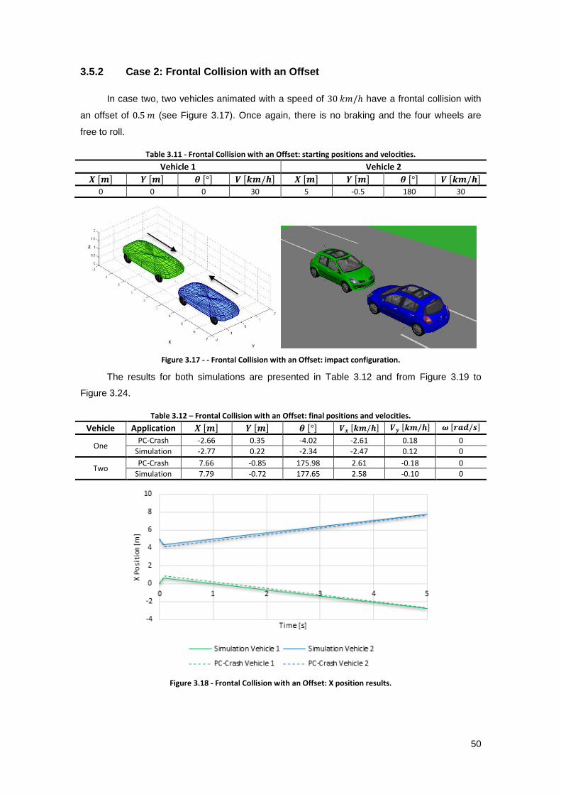
50

3.5.2 Case 2: Frontal Collision with an Offset

In case two, two vehicles animated with a speed of have a frontal collision with

an offset of (see Figure 3.17). Once again, there is no braking and the four wheels are

free to roll.

Table 3.11 - Frontal Collision with an Offset: starting positions and velocities.

Vehicle 1 Vehicle 2

[ ] [ ] [ ] [ ] [ ] [ ] [ ] [ ]

0 0 0 30 5 -0.5 180 30

Figure 3.17 - - Frontal Collision with an Offset: impact configuration.

The results for both simulations are presented in Table 3.12 and from Figure 3.19 to

Figure 3.24.

Table 3.12 – Frontal Collision with an Offset: final positions and velocities.


One PC-Crash -2.66 0.35 -4.02 -2.61 0.18 0

Simulation -2.77 0.22 -2.34 -2.47 0.12 0

Two PC-Crash 7.66 -0.85 175.98 2.61 -0.18 0

Simulation 7.79 -0.72 177.65 2.58 -0.10 0

Figure 3.18 - Frontal Collision with an Offset: X position results.

51

Figure 3.19 - Frontal Collision with an Offset: X velocity results.

Figure 3.20 - Frontal Collision with an Offset: Y position results.

Figure 3.21 - Frontal Collision with an Offset: Y velocity results.

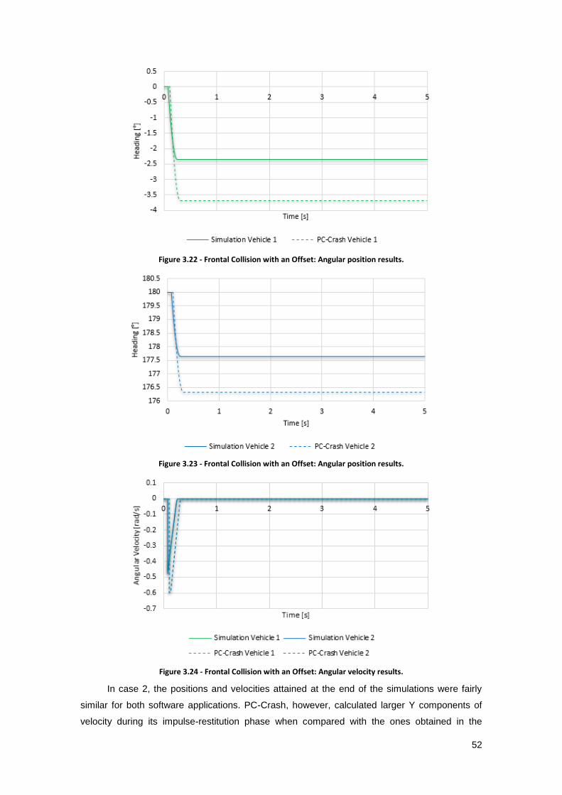
52

Figure 3.22 - Frontal Collision with an Offset: Angular position results.

Figure 3.23 - Frontal Collision with an Offset: Angular position results.

Figure 3.24 - Frontal Collision with an Offset: Angular velocity results.

In case 2, the positions and velocities attained at the end of the simulations were fairly

similar for both software applications. PC-Crash, however, calculated larger Y components of

velocity during its impulse-restitution phase when compared with the ones obtained in the

53

contact phase of the simulation. Even though PC-Crash calculated lower Y components of

velocity during the motion after the impulse-restitution phase, their higher values during that

phase translate themselves into higher values for the Y position at the end of the simulation. A

major difference between the simulations is the contact phase itself. According to Datentechnik

(2011), when PC-Crash detects contact between vehicles it doesn’t apply the impulse-restitution

model immediately, but rather waits 15 to 60 milliseconds in order to represent the crush of the

vehicles, resulting in the almost 1 meter of penetration shown in Figure 3.25.

Figure 3.25 - Frontal Collision with Offset: maximum penetration between the vehicles (t=0.10s).

This doesn’t happen with the continuous contact force model implemented in the

simulation, which forces the vehicles to quickly separate and the maximum penetration is 83

millimeters.

3.5.3 Case 3: Side Collision

In case three, a vehicle animated with a speed of impacts the side of another

vehicle animated with a speed of . It’s considered that the four wheels are locked after

impact.

Table 3.13 – Side Collision: starting positions and velocities.

Vehicle 1 Vehicle 2

[ ] [ ] [ ] [ ] [ ] [ ] [ ] [ ]

0 0 0 50 5 3 90 30

Figure 3.26 – Side Collision: impact configuration.

The results for both simulations are presented in Table 3.14 and from Figure 3.29 to

Figure 3.33.

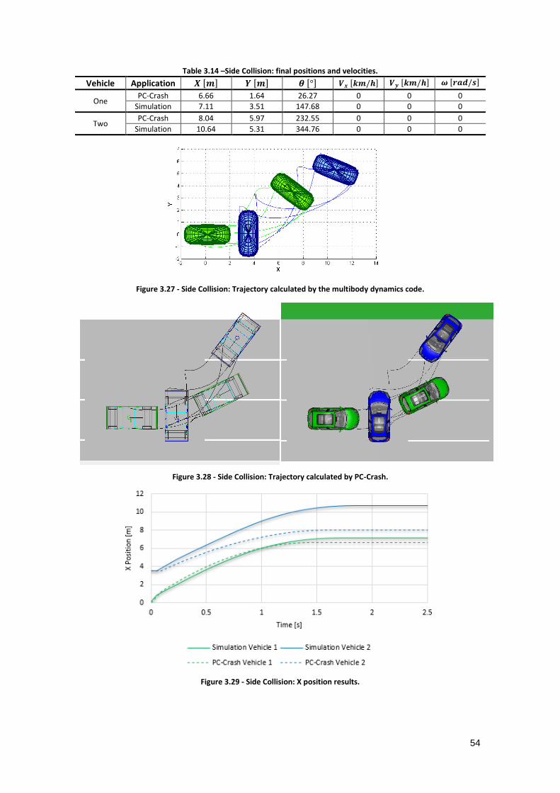
54

Table 3.14 –Side Collision: final positions and velocities.


One PC-Crash 6.66 1.64 26.27 0 0 0

Simulation 7.11 3.51 147.68 0 0 0

Two PC-Crash 8.04 5.97 232.55 0 0 0

Simulation 10.64 5.31 344.76 0 0 0

Figure 3.27 - Side Collision: Trajectory calculated by the multibody dynamics code.

Figure 3.28 - Side Collision: Trajectory calculated by PC-Crash.

Figure 3.29 - Side Collision: X position results.

55

Figure 3.30 - Side Collision: X velocity results.

Figure 3.31 - Side Collision: Y position results.

Figure 3.32 - Side Collision: Y velocity results.

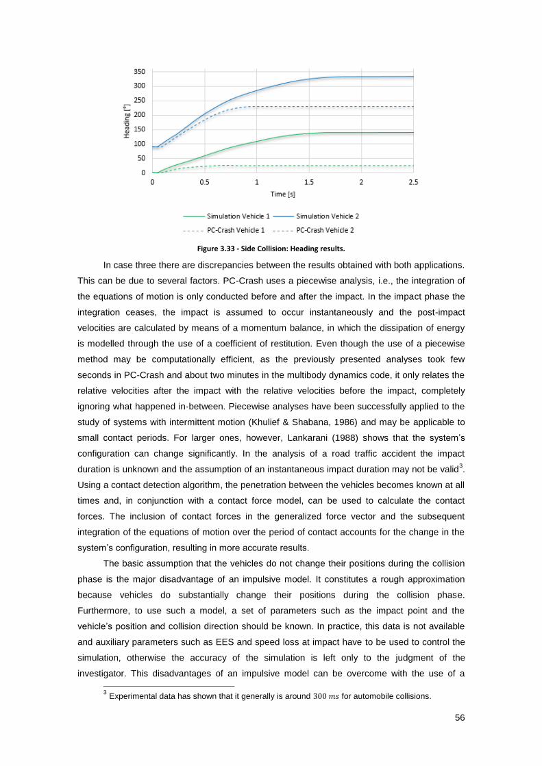
56

Figure 3.33 - Side Collision: Heading results.

In case three there are discrepancies between the results obtained with both applications.

This can be due to several factors. PC-Crash uses a piecewise analysis, i.e., the integration of

the equations of motion is only conducted before and after the impact. In the impact phase the

integration ceases, the impact is assumed to occur instantaneously and the post-impact

velocities are calculated by means of a momentum balance, in which the dissipation of energy

is modelled through the use of a coefficient of restitution. Even though the use of a piecewise

method may be computationally efficient, as the previously presented analyses took few

seconds in PC-Crash and about two minutes in the multibody dynamics code, it only relates the

relative velocities after the impact with the relative velocities before the impact, completely

ignoring what happened in-between. Piecewise analyses have been successfully applied to the

study of systems with intermittent motion (Khulief & Shabana, 1986) and may be applicable to

small contact periods. For larger ones, however, Lankarani (1988) shows that the system’s

configuration can change significantly. In the analysis of a road traffic accident the impact

duration is unknown and the assumption of an instantaneous impact duration may not be valid3.

Using a contact detection algorithm, the penetration between the vehicles becomes known at all

times and, in conjunction with a contact force model, can be used to calculate the contact

forces. The inclusion of contact forces in the generalized force vector and the subsequent

integration of the equations of motion over the period of contact accounts for the change in the

system’s configuration, resulting in more accurate results.

The basic assumption that the vehicles do not change their positions during the collision

phase is the major disadvantage of an impulsive model. It constitutes a rough approximation

because vehicles do substantially change their positions during the collision phase.

Furthermore, to use such a model, a set of parameters such as the impact point and the

vehicle’s position and collision direction should be known. In practice, this data is not available

and auxiliary parameters such as EES and speed loss at impact have to be used to control the

simulation, otherwise the accuracy of the simulation is left only to the judgment of the

investigator. This disadvantages of an impulsive model can be overcome with the use of a

3 Experimental data has shown that it generally is around for automobile collisions.

57

continuous force model. When impact occurs, the contact forces between the vehicles are

calculated and considered in the integration of the equations of motion, thereby simulating the

entire collision phase without the intervention of the investigator. On the other hand, the

continuous force model used in the present dissertation is of the Hertzian kind, i.e., the bodies

are rigid and the forces are calculated as being equivalent to those that would appear if the

bodies were pressed against each other with a degree of local elastic deformation equal to the

penetration. This model is therefore valid for small deformations and in a road traffic accident

this is not usually the case. The maximum penetration is shown in Figure 3.34. It can be seen

that whereas PC-Crash accounts for the crush of the vehicles, in the implemented multibody

dynamics code the continuous force model quickly separates the vehicles for low values of

penetration. This aspect may be a limitation of a Hertzian continuous force model applied to a

road traffic accident. A volumetric contact model, in which the contact force is proportional to the

volume of interference, or the use of deformable bodies would be more applicable to the

problem. Note that Bogdanovic, Milutinovic, Kostic & Ruskic (2012) studied the influence of

twenty input parameters and determined that the overlapping width is the parameter that most

influences trajectory errors in analysis based on Kudlich (1966) and Slibar (1966) impulsive

collision models, where linear and angular momentum are conserved and energy dissipation is

modelled by the use of a coefficient of restitution.

Additionally note that momentary discontinuities can be observed in almost all figures

concerning penetration values presented in this chapter. In certain time instants, with particular

configurations of the system, the narrow phase of contact converges to a point in which some

constraints are violated, generally the ones regarding parallelism between the normal surface

vectors. This phenomenon is however fleeting and quickly dissipates, returning the optimizer to

valid solutions. It does not appear to affect the overall motion of the system.

Figure 3.34 – Side Collision: Comparison between the maximum penetration obtained with PC-Crash (t=0.90s) and the implemented multibody dynamics code (t=0.84).

58

Finally, PC-Crash establishes a distinction between two types of impact, full impact and

sliding impact. In a full impact there is no relative movement between the vehicles at the

impulse point at the end of the compression phase. On a sliding impact the two vehicles do not

reach a common velocity at the impulse point and there is only no relative movement in the

normal direction to the contact plane at the end of the compression phase, being the vehicles

free to slide along the tangential direction. Even though it’s not clear how PC-Crash makes such

distinction for its simulations, it’s most likely based on the ratio between the tangential and

normal components of the approach velocity as in Djerassi (2009). With a continuous force

model there is no distinction between different types of impact, as different configurations of the

system lead to different penetration and contact force values.

59

4 Multi-Objective Optimization with Genetic Algorithms

Chapter 4 presents an overview of the required formulations to develop a multi-objective

optimization algorithm. The principles of genetic algorithms are reviewed, along with selection,

crossover and mutation genetic operators. The concept of multi-objective optimization is

introduced and the implemented multi-objective optimization algorithm is thoroughly analyzed.

4.1 Stages of a Genetic Algorithm

A genetic algorithm starts by randomly generating a population within specific lower and

upper bounds of each design variable. Alternatively, Deb, Reddy & Singh (2003) argues that if

there is knowledge regarding some possible good solutions, their introduction in the initial

population is helpful in achieving a faster convergence. Then, the genetic algorithm enters an

iterative process of updating the population through the use of three genetic operators

(selection, crossover and mutation), until one or more termination criteria are met. In each

generation, the members of the population are evaluated regarding their fitness towards a

certain objective and the selection operator chooses above average solutions to fill the mating

pool. With the solutions on the mating pool (parents), the crossover operator creates one or

more solutions (offspring) by exchanging information between them. A portion of the solutions

are then perturbed by a mutation operator, allowing the genetic algorithm to explore different

areas of the design space. In a concise manner, a genetic algorithm is a population-based

stochastic search procedure which iteratively emphasizes its more fit population members,

which are then recombined and perturbed in the hope of creating new and better populations.

In classic genetic algorithms each chromosome is encoded using binary representation.

Tree encoding can also be used, in which every chromosome is denoted by a tree of objects,

such as functions or commands in a programming language (Koza, 1992). In Back, Fogel &

Michalewicz (1997) it’s argued that a real representation is better for optimization problems

involving real values. This dissertation adopts a real representation for chromosomes, in what is

henceforth referred as continuous genetic algorithm.

4.2 Selection Operators

The selection operator plays a crucial role in a genetic algorithm. It should ensure the

selection of higher fitness individuals for reproduction more often than lower fitness ones, so

that the population keeps improving throughout the generations and, at the same time, it must

guarantee that the population doesn’t become dominated by the higher fitness individuals, as

that could lead to convergence on a local minimum.

The roulette wheel selection was first introduced by Holland (1975). It quantifies the

probability of an individual being selected for reproduction by dividing its fitness by the total

fitness of the population.

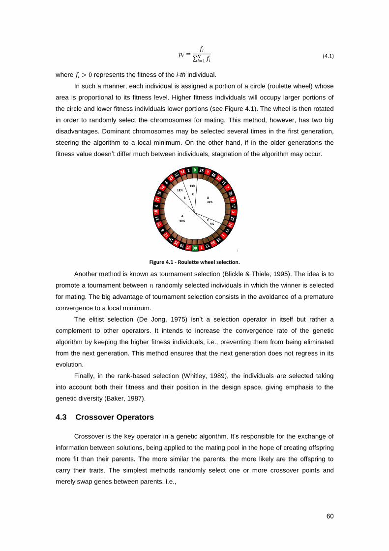
60

∑

(4.1)

where represents the fitness of the i-th individual.

In such a manner, each individual is assigned a portion of a circle (roulette wheel) whose

area is proportional to its fitness level. Higher fitness individuals will occupy larger portions of

the circle and lower fitness individuals lower portions (see Figure 4.1). The wheel is then rotated

in order to randomly select the chromosomes for mating. This method, however, has two big

disadvantages. Dominant chromosomes may be selected several times in the first generation,

steering the algorithm to a local minimum. On the other hand, if in the older generations the

fitness value doesn’t differ much between individuals, stagnation of the algorithm may occur.

Figure 4.1 - Roulette wheel selection.

Another method is known as tournament selection (Blickle & Thiele, 1995). The idea is to

promote a tournament between randomly selected individuals in which the winner is selected

for mating. The big advantage of tournament selection consists in the avoidance of a premature

convergence to a local minimum.

The elitist selection (De Jong, 1975) isn’t a selection operator in itself but rather a

complement to other operators. It intends to increase the convergence rate of the genetic

algorithm by keeping the higher fitness individuals, i.e., preventing them from being eliminated

from the next generation. This method ensures that the next generation does not regress in its

evolution.

Finally, in the rank-based selection (Whitley, 1989), the individuals are selected taking

into account both their fitness and their position in the design space, giving emphasis to the

genetic diversity (Baker, 1987).

4.3 Crossover Operators

Crossover is the key operator in a genetic algorithm. It’s responsible for the exchange of

information between solutions, being applied to the mating pool in the hope of creating offspring

more fit than their parents. The more similar the parents, the more likely are the offspring to

carry their traits. The simplest methods randomly select one or more crossover points and

merely swap genes between parents, i.e.,

61

[ ]

[ ]

[ ]

[ ]

(4.2)

The uniform crossover method states that for each gene, the parent that will contribute to

it should be chosen randomly. Thus, one goes down the line of the chromosomes’ genes and,

at each gene, randomly decide whether or not to swap information between the two parents.

The main problem with these methods is that they rely solely on mutation to introduce new

genetic material, i.e., no new information is introduced in the population as the values that were

randomly generated in the initial population are propagated to the following generations.

Blending methods were developed to overcome this issue (Radcliff, 1991), combining

variable values from the two parents into new variable values that are carried over to the

offspring. Radcliff’s blending method can be expressed as

( ) (4.3)

where is a randomly generated number between 0 and 1.This method, however, doesn’t allow

the introduction of values beyond the bounds already present in the population. Heuristic

crossover (Michalewicz, 1994) solved this problem by setting

( ) (4.4)

In order not to stray too far from the values in the population, the BLX-α (Eshelman &

Shaffer, 1993) begins by choosing a parameter, , outside of the bounds of the two parent

variables, where the new offspring variable is allowed to lie.

The simulated binary crossover (Deb & Agrawal, 1995) generates two offspring from two

parent solutions. First, a random number between 0 and 1 is created. Then, a parameter

representing the ratio of the absolute difference in offspring values to that of the parents is

calculated as

{

( )

(

( ))

(4.5)

where is a non-negative user defined parameter. Large values of increase the probability

of creating near-parent solutions and low values of the opposite. The two offspring are then

calculated as

( ) ( )

( ) ( )

(4.6)

The crossover operator implemented in this dissertation is the simulated binary

crossover (Deb & Agrawal, 1995).

62

4.4 Mutation Operators

Mutation operators force the genetic algorithm to look for solutions in unexplored areas of

the objective space by randomly introducing changes, or mutations, in some chromosomes,

thus preventing the algorithm from converging to a local minimum. Mutation plays the role of

recovering lost genetic material as well as randomly distributing genetic information and

maintaining genetic diversity in the population. If the role of crossover is to exploit current

solutions to find better ones, the role of mutation is to foster the exploration of the whole search

space. For a binary genetic algorithm, the mutation process is as simple as changing one bit

from 0 to 1 or vice versa. The string would still be very similar but the new individual would have

completely different objective function values. In a continuous genetic algorithm, a common

method for mutation is to add a normally distributed random number to the variable selected for

mutation.

( ) (4.7)

Mutation is not commonly applied to the offspring of the penultimate generation.

4.5 Elitism

If elitism is added to the genetic algorithm, the best chromosome or the few top ranked

chromosomes are copied to the new population. This prevents the top ranked individuals of

being lost if they’re not selected for mating or if mutation destroys them. Note that if elitism is

introduced, the elite solutions should not be mutated. Mutation is also not commonly applied to

the offspring of the penultimate generation. For information concerning crossover operators in

binary encoded genetic algorithms see Spears (1998) and for continuous genetic algorithms

refer to Adewuya (1996).

4.6 Multi-Objective Optimization

A multi-objective optimization problem involves a number of objective functions which are

to be either minimized or maximized. The objective functions are often conflicting, since the

improvement of one objective can worsen another. Consequently, the optimal solution isn’t a

single point, as in the case of single-objective optimization, but rather a set of points called

Pareto optimal. Figure 4.2 illustrates this concept in the minimization of two objective functions.

Solution D is worse than solution C regarding both objectives. Even though solutions A and B

have the same value regarding , B is worse than A regarding . Solutions A, C and E cannot

be compared, as a gain in an objective happens only due to a sacrifice in the other objective.

These three points are called Pareto optimal or non-dominated solutions (Pareto, 1896) and the

orange line represents the Pareto front. A solution is called non-dominated if and only if it

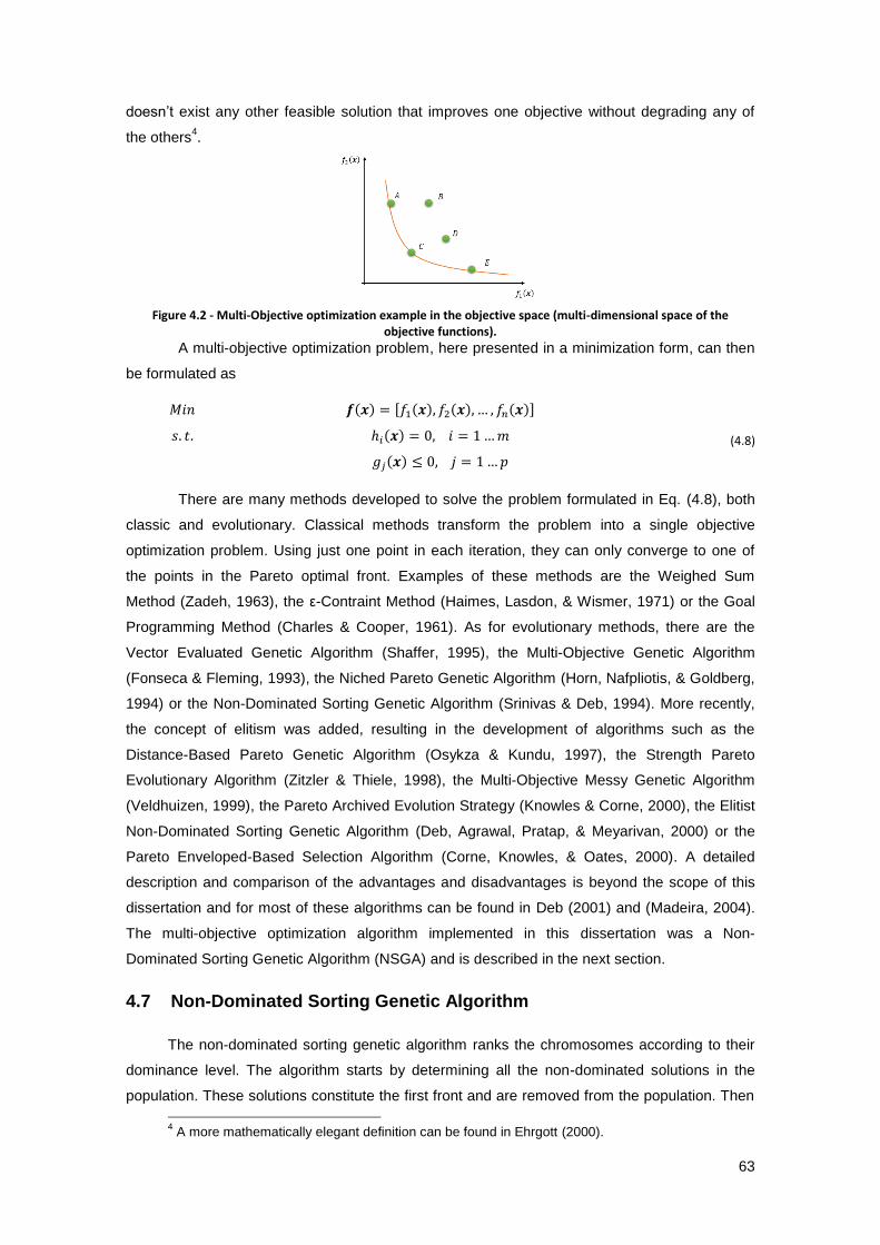
63

doesn’t exist any other feasible solution that improves one objective without degrading any of

the others4.

Figure 4.2 - Multi-Objective optimization example in the objective space (multi-dimensional space of the objective functions).

A multi-objective optimization problem, here presented in a minimization form, can then

be formulated as

( ) [ ( ) ( ) ( )]

(4.8) ( )

( )

There are many methods developed to solve the problem formulated in Eq. (4.8), both

classic and evolutionary. Classical methods transform the problem into a single objective

optimization problem. Using just one point in each iteration, they can only converge to one of

the points in the Pareto optimal front. Examples of these methods are the Weighed Sum

Method (Zadeh, 1963), the ε-Contraint Method (Haimes, Lasdon, & Wismer, 1971) or the Goal

Programming Method (Charles & Cooper, 1961). As for evolutionary methods, there are the

Vector Evaluated Genetic Algorithm (Shaffer, 1995), the Multi-Objective Genetic Algorithm

(Fonseca & Fleming, 1993), the Niched Pareto Genetic Algorithm (Horn, Nafpliotis, & Goldberg,

1994) or the Non-Dominated Sorting Genetic Algorithm (Srinivas & Deb, 1994). More recently,

the concept of elitism was added, resulting in the development of algorithms such as the

Distance-Based Pareto Genetic Algorithm (Osykza & Kundu, 1997), the Strength Pareto

Evolutionary Algorithm (Zitzler & Thiele, 1998), the Multi-Objective Messy Genetic Algorithm

(Veldhuizen, 1999), the Pareto Archived Evolution Strategy (Knowles & Corne, 2000), the Elitist

Non-Dominated Sorting Genetic Algorithm (Deb, Agrawal, Pratap, & Meyarivan, 2000) or the

Pareto Enveloped-Based Selection Algorithm (Corne, Knowles, & Oates, 2000). A detailed

description and comparison of the advantages and disadvantages is beyond the scope of this

dissertation and for most of these algorithms can be found in Deb (2001) and (Madeira, 2004).

The multi-objective optimization algorithm implemented in this dissertation was a Non-

Dominated Sorting Genetic Algorithm (NSGA) and is described in the next section.

4.7 Non-Dominated Sorting Genetic Algorithm

The non-dominated sorting genetic algorithm ranks the chromosomes according to their

dominance level. The algorithm starts by determining all the non-dominated solutions in the

population. These solutions constitute the first front and are removed from the population. Then

4 A more mathematically elegant definition can be found in Ehrgott (2000).

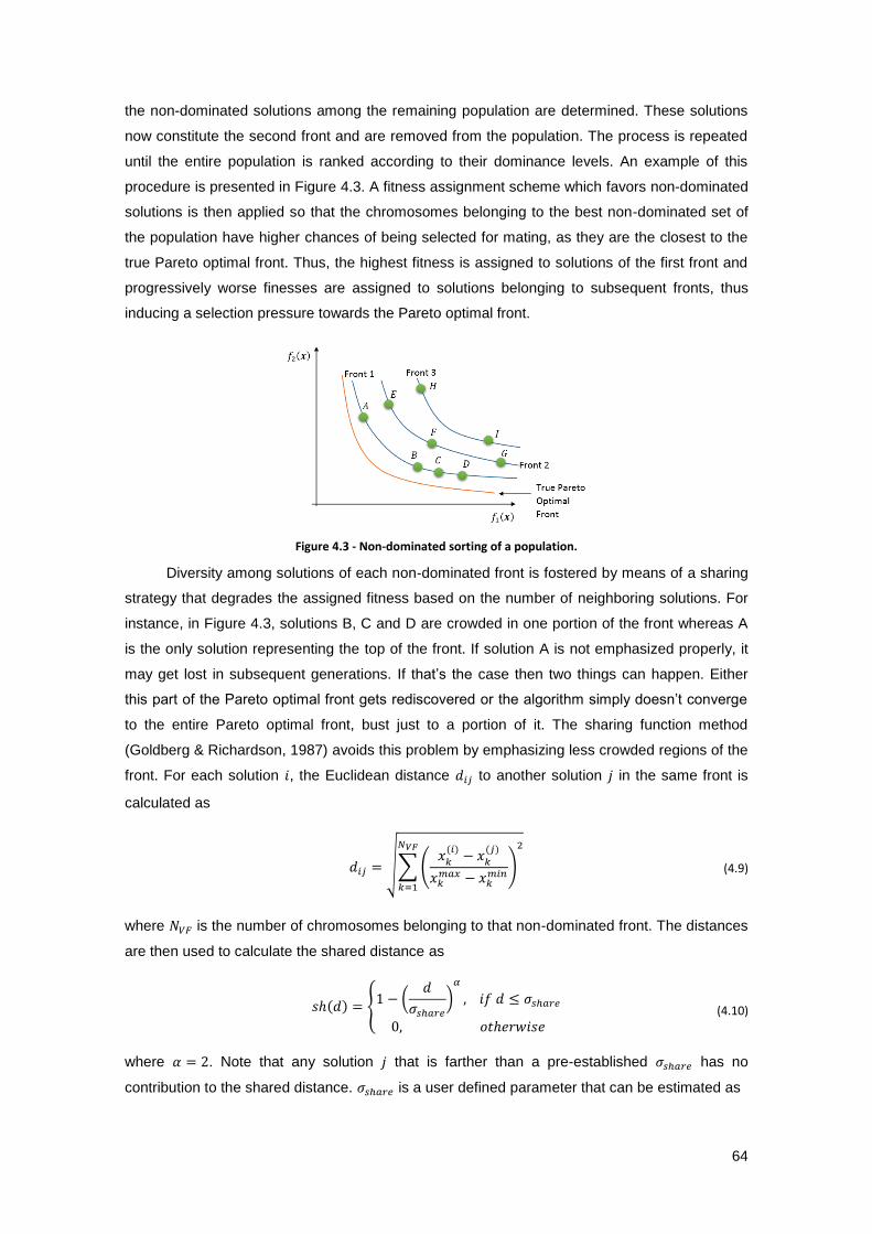
64

the non-dominated solutions among the remaining population are determined. These solutions

now constitute the second front and are removed from the population. The process is repeated

until the entire population is ranked according to their dominance levels. An example of this

procedure is presented in Figure 4.3. A fitness assignment scheme which favors non-dominated

solutions is then applied so that the chromosomes belonging to the best non-dominated set of

the population have higher chances of being selected for mating, as they are the closest to the

true Pareto optimal front. Thus, the highest fitness is assigned to solutions of the first front and

progressively worse finesses are assigned to solutions belonging to subsequent fronts, thus

inducing a selection pressure towards the Pareto optimal front.

Figure 4.3 - Non-dominated sorting of a population.

Diversity among solutions of each non-dominated front is fostered by means of a sharing

strategy that degrades the assigned fitness based on the number of neighboring solutions. For

instance, in Figure 4.3, solutions B, C and D are crowded in one portion of the front whereas A

is the only solution representing the top of the front. If solution A is not emphasized properly, it

may get lost in subsequent generations. If that’s the case then two things can happen. Either

this part of the Pareto optimal front gets rediscovered or the algorithm simply doesn’t converge

to the entire Pareto optimal front, bust just to a portion of it. The sharing function method

(Goldberg & Richardson, 1987) avoids this problem by emphasizing less crowded regions of the

front. For each solution , the Euclidean distance to another solution in the same front is

calculated as

√∑( ( )

( )

)

(4.9)

where is the number of chromosomes belonging to that non-dominated front. The distances

are then used to calculate the shared distance as

( ) { (

)

(4.10)

where . Note that any solution that is farther than a pre-established has no

contribution to the shared distance. is a user defined parameter that can be estimated as

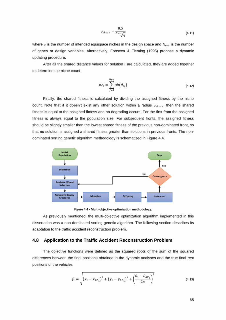
65

√

(4.11)

where is the number of intended equispace niches in the design space and is the number

of genes or design variables. Alternatively, Fonseca & Fleming (1995) propose a dynamic

updating procedure.

After all the shared distance values for solution are calculated, they are added together

to determine the niche count

∑ ( )

(4.12)

Finally, the shared fitness is calculated by dividing the assigned fitness by the niche

count. Note that if it doesn’t exist any other solution within a radius , then the shared

fitness is equal to the assigned fitness and no degrading occurs. For the first front the assigned

fitness is always equal to the population size. For subsequent fronts, the assigned fitness

should be slightly smaller than the lowest shared fitness of the previous non-dominated front, so

that no solution is assigned a shared fitness greater than solutions in previous fronts. The non-

dominated sorting genetic algorithm methodology is schematized in Figure 4.4.

Figure 4.4 - Multi-objective optimization methodology.

As previously mentioned, the multi-objective optimization algorithm implemented in this

dissertation was a non-dominated sorting genetic algorithm. The following section describes its

adaptation to the traffic accident reconstruction problem.

4.8 Application to the Traffic Accident Reconstruction Problem

The objective functions were defined as the squared roots of the sum of the squared

differences between the final positions obtained in the dynamic analyses and the true final rest

positions of the vehicles

√( ) ( )

(

)

(4.13)

66

√( ) ( )

(

)

(4.14)

where ( ) are the final positions of vehicle obtained in the dynamic analysis and

( ) are the real final positions of vehicle , recorded by the police authorities.

The non-dominated sorting genetic algorithm uses the roulette-wheel selection operator

applied to the shared fitness, thus ensuring that solutions in the best non-dominated front have

better chances of being selected for mating and, when in conjunction with the sharing function

method, that less crowded solutions are also more likely to be selected. To foster genetic

diversity among solutions a restriction was added to the crossover, this being that a

chromosome cannot mate with itself, i.e., each new solution must be an offspring of two

different parents. Furthermore, with both parents chosen, the crossover operator cannot be

freely applied, as that could originate solutions with overlapped starting positions or that simply

are not in a collision course, rendering the dynamic analysis meaningless. The first attempt at

solving this issue was to directly affect the fitness of non-colliding solutions. This procedure,

however, was unsuccessful as even with a crippled fitness the non-colliding solutions rapidly

took over the majority of the population and only a few colliding solutions would remain, not

being representative of the design space. For this reason, an iterative process was

implemented in order to guarantee that each generated solution (be it in the randomly

generated initial population, offspring or mutated solutions) obeys two constraints, these being

to correspond to a non-overlapped starting position and to be a solution in which there is indeed

a collision between the vehicles.

Genetic algorithms are very flexible. That flexibility, however, transfers to the programmer

the burden of choosing the appropriate operators in order to create an efficient and consistent

search (Radcliff, 1991), as the objective is not only to find a set of solutions which lie in the

Pareto-optimal front, but also to find a set of solutions that are diverse enough to represent the

entire range of the Pareto-optimal front. Several mutation operators were tested, being the one

described in Deb & Deb (2012) the final choice for its ability to introduce diversity among the

solutions of the particular problem dealt in this dissertation. For a given solution , its mutated

form for a particular variable is created as follows

{ (

)

(

) (4.15)

where is a randomly generated number between 0 and 1 and one of the two parameters is

calculated as

( )

(4.16)

( ( ))

(4.17)

and is a user specified variable between 20 and 100. In the multi-objective optimization

algorithm implemented in this dissertation, mutation is not applied to the final 4 generations.

67

5 Optimization of Road Traffic Accidents

Chapter 5 presents examples of application of the developed multi-objective optimization

methodology to the reconstruction of road traffic accidents, by means of a genetic algorithm that

maintains diversity among the population while guiding it to the optimal Pareto set. The current

traffic accident reconstruction procedure is explained and an emphasis is given as to what multi-

objective optimization can offer to the field. A case study of an accident is presented and used

as the real solution for five different examples of multi-objective optimization. The results show

that multi-objective optimization can and should be considered as a valid tool for the future of

traffic accident reconstruction.

5.1 Accident Reconstruction

An accident reconstruction is the investigation of a road traffic accident, conducted in

order to determine how the accident occurred. The field of accident reconstruction deals with

the estimation of impact conditions based on post-accident information in order to determine

how the vehicles were moving before and during the collision.

When an accident occurs, the preliminary investigation is often carried out by the police

authorities, gathering basic information in an accident report such as information regarding

vehicles, statements from drivers and witnesses, photographs and a scale drawing of the

scene. The scale drawing is made with detailed measurements to careful document the location

of the final rest positions of the vehicles, skid marks, scratch or gouging on the road surface or

any other evidence found such as debris or human fluids. In accidents with injured or fatal

victims, a medical doctor performs a thorough examination of the injuries. Some police

departments have rudimentary knowledge regarding motor vehicle accidents and may attempt

to perform some initial reconstruction, calculating vehicle speeds and points of impact. The goal

of the police force is to determine whether or not any driver should be charged with traffic act

offenses. On the other hand, insurance companies have concerns regarding liability for accident

causation and resultant property damage and injury claims. In cases with fatal or severe victims,

lawyers or court officials hire independent experts, typically engineers, to conduct a further

reconstruction of the accident.

The traffic accident investigator requires all the previous information gathered by the

police force, statements from drivers and witnesses and hospital reports. This information, along

with an examination of the scene and an inspection of the vehicles to measure crush profiles

and check for failure of mechanical components, allows the investigator to perform a valid

reconstruction of the accident (note that the accident reconstruction is only as good as the

evidence allows). His goal is to describe the pre-impact5 events in terms of each vehicle’s

position on the road, heading and speed. Several questions can arise. Were they speeding?

Who crossed the centerline? Could the pedestrian be seen? Who was driving? Could they have

5 Often, the lack of evidence regarding pre-impact motion only enables the reconstruction from the

impact event onwards.

68

avoided the accident if they were travelling at the speed limit? Was the pedestrian crossing the

road in the crosswalk? Could the drivers perceive the hazard in front of them? Were there

environmental factors that contributed to the accident? Did they stop at the stop sign? What

happened? To properly answer these questions, an accident reconstruction must be performed.

At NIAR (Dias, Portal, & Paulino, 2012), the accident investigation unit of the University of

Lisbon, the computational reconstruction of road traffic accidents is treated as an iterative

process as outlined in the flowchart in Figure 5.1, being the pre-impact positions and velocities

the variable parameters.

Figure 5.1 - Accident reconstruction process.

The reconstruction process can be divided into three steps: evidence gathering, dynamic

analysis and evaluation of results. The scale drawing is used to create a 3D scenario of the

accident scene. Through the analysis of the crush profile it’s possible to determine the relative

orientation of the vehicles at the moment of impact and to perform a gross estimation of the

travelling speeds. Then, a forward simulation is performed and checked for compatibility with

the recorded rest positions of the vehicles, their amount of crush (the structural damage is often

described using crush or EES6 values and can be evaluated by examining the vehicles or by

using photographs of the deformed areas), consistency with evidence found on the scene and

witnesses’ statements regarding post-impact motion. If these criterion are not satisfied, the pre-

impact parameters are modified and the process is repeated iteratively until a simulation

consistent with the evidence is found. In such a way, the reconstruction process involves

6 Energy Equivalent Speed: plastic deformation energy expressed as a virtual velocity value at

which a vehicle would have to impact a rigid wall in order to register the same amount of structural damage of the crashed vehicle.

69

subjective evaluations of pre-impact conditions, requiring several7 simulations until a solution

with results consistent with the physical evidences is found. If several pre-impact parameters

are unknown, the reconstruction can take a good deal of time. The reconstruction program used

at NIAR is PC-Crash, a commercial software widely accepted in the accident reconstruction field

and validated in international conferences, respectively, the program itself (Cliff & Montgomery,

1996) and the use of multibody dynamics in the reconstruction of road traffic accidents (Moser,

Steffan, & Kasanicky, 1999). Containing an extensive database of vehicle models it also allows

to animate the results in video format, which is useful in court proceedings, since it

demonstrates the opinion of the investigator in a form easily understood by a judge.

5.2 The Role of Multi-Objective Optimization in Accident Reconstruction

If a road traffic accident is treated as an engineering problem, its solution is non-unique,

as there are several impact configurations and velocities that lead to the same final rest

positions. For instance, in a pedestrian run-over this aspect is critical. Generally, only the rest

position of the pedestrian is known and no matter what impact point is considered, it’s possible

to find an impact velocity that throws the pedestrian to his rest position. The differences

between the spread of solutions lie in the injuries sustained by the pedestrian, i.e., whether or

not they are consistent with the collision forces. Similarly, in a two-vehicle accident the rest

positions can be achieved through many impact configurations. However, only a few of those

are consistent with the deformations, EES value (Rovidz & Melegh, 2003), possible skid marks

and other evidence on the pavement.

Most traffic accidents are reconstructed using iterative methods. A forward simulation is

performed and the compatibility of the results obtained with the accident evidences such as

vehicle damage or skid marks is analyzed. Optimization techniques have also been utilized in

Moser & Steffan (1998), Cliff & Moser (2001), Steffan, Moser, Spek & Makkinga (2007) and

Martins & Neto (2008). However, their approach to the problem is single-objective, i.e., the goal

of the optimization is to minimize a weighted total error, using the least mean squares method,

as follows

√∑ ( )

∑

(5.1)

where is the weighting of each parameter (0 to 100%) and is the difference between

the real and the calculated parameter values.

This method minimizes a weighted total error by automatically varying a set of user

defined parameters and then comparing the simulation results with the accident data.

Therefore, the quality of the simulation results is expressed solely by an error determined on the

basis of the difference between the rest positions obtained by the simulation and the real ones

(post-impact trajectories can also be included). Thus, the accident investigator associates

weights with each objective (which are often subjective and dependent of non-technical

7 Often dozens and sometimes well into the hundreds.

70

knowledge and qualitative experience), the reconstruction process is reduced to a single

objective problem and its solution will consist of a single optimal point. If the result is not

satisfactory, the preferences of the accident investigator change and the whole optimization

process must be reapplied.

The main problem with this single-objective method is that the assumption has been

made that the lower the difference between the simulation results and the real accident data,

the closer the simulation is to the real case, whereas in reality there is no guarantee that the

global minimum of the problem is the true solution of the traffic accident reconstruction. Using a

multi-objective approach the result is not a single solution (note that even in the final population

of a single-objective problem solved through a genetic algorithm chances are that the entirety of

the population will be clustered around the global minimum) but rather a Pareto curve with

several solutions, from which one consistent with the accident data can be chosen, i.e., the

trade-off property between non-dominated solutions of a multi-objective optimization problem

makes it the ideal vessel to find a wide variety of solutions before making a final choice. The

investigator now faces a dilemma. Since a number of solutions are optimal, which one should

he choose? This is not an easy question to answer and the final decision involves a large

amount of technical, qualitative and experience driven background. However, the simple fact of

having a set of trade-off solutions as opposed to a single optimal solution, makes it possible to

evaluate the pros and cons of each one and compare them to make a proper decision.

5.3 Application to Traffic Accident Reconstruction

The following sections will present examples of application of the developed multi-

objective optimization algorithm to the accident reconstruction problem. A case study of an

accident is presented and used as the real solution for five different possibilities of optimization.

The results are shown in terms of vehicle configuration at the time of first detected contact.

5.3.1 Problem Definition

One of the most common motor vehicle accidents is the side impact on a crossroads due

to a priority fault. In it, one of the drivers doesn’t stop at the red light or disrespects priority rules

and crashes into the side flank of another vehicle. This example was presented in Section 3.5.3

and will be used as a cased study for the multi-objective optimization process.

The objective functions are the differences between the vehicle’s rest positions obtained

in the dynamic simulation and the real rest positions of the vehicles, given by

√( ) ( )

(

)

(5.2)

√( ) ( )

(

)

(5.3)

where ( ) are the final positions of vehicle obtained in the dynamic analysis and

( ) are the real final positions of vehicle , recorded by the police authorities. This same

71

problem will be solved in five different cases, where the differences between them lie in which

design variables are being used in the optimization process. Albeit using different groups of

design variables, their goal is the same, i.e., to determine which set of parameters at the

moment of impact are better correlated with the rest positions of the vehicles. In the presented

results the blue dots represent the non-dominated solutions and the green dots the dominated

ones. Furthermore, the trajectories of some solutions are presented, in which the grey and

colored rectangles represent the collision and final positions of the case study, respectively.

Table 5.1 -Problem: initial, collision and rest positions.

Vehicle One Two

Positions [ ] [ ] [ ] [ ] [ ] [ ] [ ] [ ]

Start 0 0 0 50 3.5 0 90 30

Collision 0.83 0 0 50 3.5 0.5 90 30

Rest 7.11 3.51 147.68 0 10.64 5.31 344.77 0

Note that for this example it’s considered that there are no steering maneuvers and that

all four wheels are locked after the impact.

5.3.2 Case 1: Velocity Optimization

When an accident is severe enough to generate a lawsuit there is often a police report

containing a field sketch with detailed measurements of the vehicle’s rest positions, be it done

by the triangle measuring procedure or the right angle coordinate procedure (Tomasch, 2004).

Figure 5.2 - Measurement Procedures: triangulation method (left) and coordinates method (right).

In this sketch it’s often indicated a probable point of collision that must be tested as a

possible impact location. Alternative impact points can also be given by witnesses or by a

sudden change in skid mark direction, as this feature is indicative of a collision.

72

Figure 5.3 - Field Sketch: probable impact point (X) and change in skid mark direction.

Case 1 deals with this specific situation, i.e., the analysis of known probable impact

points. For a given impact point, the algorithm will try to determine which set of velocities is

better correlated with the rest positions. Note that pre-impact velocities have a very strong

influence on the post-impact motion and in the amount of damage resulting from the accident.

The increasing use of dash cams to tackle the current epidemic of road rage in Eastern

countries (Sansone & Sansone, 2010) also transforms the accident reconstruction in a problem

of determining the travelling velocities, for cases in which cameras are not equipped with GPS.

The minimization problem is formulated in Eq. (5.4).

Min √( ) ( )

(

)

(5.4)

√( ) ( )

(

)

S.t.

The multi-objective optimization process was successful, being the algorithm capable of

determining impact conditions in the vicinity of real solution. The results are presented in Figure

5.4, Table 5.2, Table 5.3, and Figure 5.5.

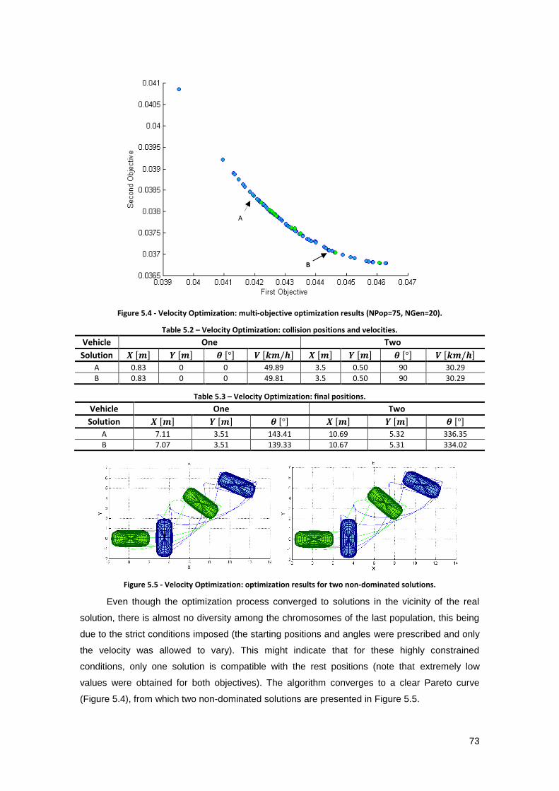
73

Figure 5.4 - Velocity Optimization: multi-objective optimization results (NPop=75, NGen=20).

Table 5.2 – Velocity Optimization: collision positions and velocities.

Vehicle One Two

Solution [ ] [ ] [ ] [ ] [ ] [ ] [ ] [ ]

A 0.83 0 0 49.89 3.5 0.50 90 30.29

B 0.83 0 0 49.81 3.5 0.50 90 30.29

Table 5.3 – Velocity Optimization: final positions.

Vehicle One Two

Solution [ ] [ ] [ ] [ ] [ ] [ ]

A 7.11 3.51 143.41 10.69 5.32 336.35

B 7.07 3.51 139.33 10.67 5.31 334.02

Figure 5.5 - Velocity Optimization: optimization results for two non-dominated solutions.

Even though the optimization process converged to solutions in the vicinity of the real

solution, there is almost no diversity among the chromosomes of the last population, this being

due to the strict conditions imposed (the starting positions and angles were prescribed and only

the velocity was allowed to vary). This might indicate that for these highly constrained

conditions, only one solution is compatible with the rest positions (note that extremely low

values were obtained for both objectives). The algorithm converges to a clear Pareto curve

(Figure 5.4), from which two non-dominated solutions are presented in Figure 5.5.

A

B

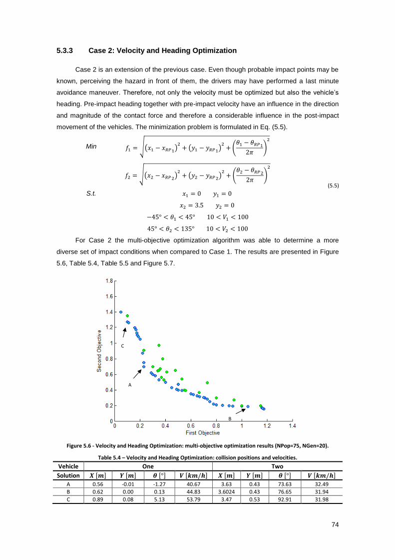
74

5.3.3 Case 2: Velocity and Heading Optimization

Case 2 is an extension of the previous case. Even though probable impact points may be

known, perceiving the hazard in front of them, the drivers may have performed a last minute

avoidance maneuver. Therefore, not only the velocity must be optimized but also the vehicle’s

heading. Pre-impact heading together with pre-impact velocity have an influence in the direction

and magnitude of the contact force and therefore a considerable influence in the post-impact

movement of the vehicles. The minimization problem is formulated in Eq. (5.5).

Min √( ) ( )

(

)

(5.5)

√( ) ( )

(

)

S.t.

For Case 2 the multi-objective optimization algorithm was able to determine a more

diverse set of impact conditions when compared to Case 1. The results are presented in Figure

5.6, Table 5.4, Table 5.5 and Figure 5.7.

Figure 5.6 - Velocity and Heading Optimization: multi-objective optimization results (NPop=75, NGen=20).

Table 5.4 – Velocity and Heading Optimization: collision positions and velocities.

Vehicle One Two

Solution [ ] [ ] [ ] [ ] [ ] [ ] [ ] [ ]

A 0.56 -0.01 -1.27 40.67 3.63 0.43 73.63 32.49

B 0.62 0.00 0.13 44.83 3.6024 0.43 76.65 31.94

C 0.89 0.08 5.13 53.79 3.47 0.53 92.91 31.98

A

B

A

C

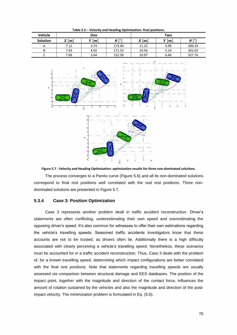
75

Table 5.5 – Velocity and Heading Optimization: final positions.

Vehicle One Two

Solution [ ] [ ] [ ] [ ] [ ] [ ]

A 7.12 3.74 173.40 11.22 4.99 306.33

B 7.93 4.02 171.53 10.56 5.14 341.03

C 7.06 3.64 152.30 10.97 6.46 327.76

Figure 5.7 - Velocity and Heading Optimization: optimization results for three non-dominated solutions.

The process converges to a Pareto curve (Figure 5.6) and all its non-dominated solutions

correspond to final rest positions well correlated with the real rest positions. Three non-

dominated solutions are presented in Figure 5.7.

5.3.4 Case 3: Position Optimization

Case 3 represents another problem dealt in traffic accident reconstruction. Driver’s

statements are often conflicting, underestimating their own speed and overestimating the

opposing driver’s speed. It’s also common for witnesses to offer their own estimations regarding

the vehicle’s travelling speeds. Seasoned traffic accidents investigators know that these

accounts are not to be trusted, as drivers often lie. Additionally there is a high difficulty

associated with clearly perceiving a vehicle’s travelling speed. Nonetheless, these scenarios

must be accounted for in a traffic accident reconstruction. Thus, Case 3 deals with the problem

of, for a known travelling speed, determining which impact configurations are better correlated

with the final rest positions. Note that statements regarding travelling speeds are usually

assessed via comparison between structural damage and EES databases. The position of the

impact point, together with the magnitude and direction of the contact force, influences the

amount of rotation sustained by the vehicles and also the magnitude and direction of the post-

impact velocity. The minimization problem is formulated in Eq. (5.6).

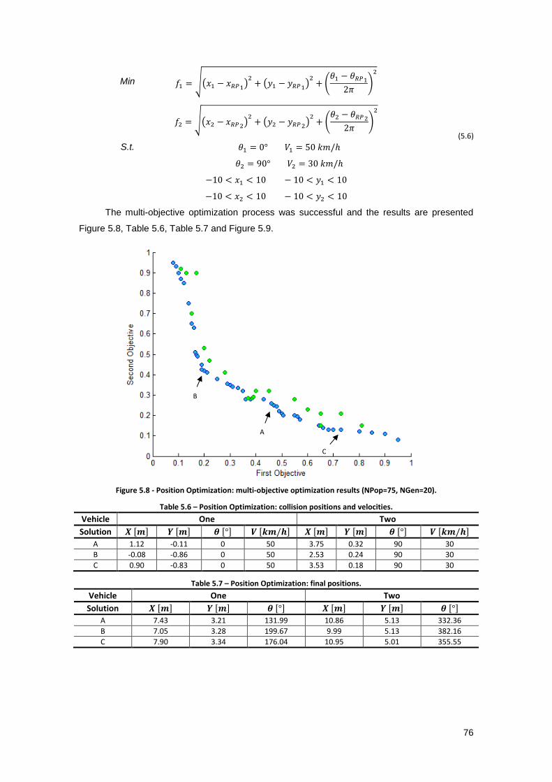
76

Min √( ) ( )

(

)

(5.6)

√( ) ( )

(

)

S.t.

The multi-objective optimization process was successful and the results are presented

Figure 5.8, Table 5.6, Table 5.7 and Figure 5.9.

Figure 5.8 - Position Optimization: multi-objective optimization results (NPop=75, NGen=20).

Table 5.6 – Position Optimization: collision positions and velocities.

Vehicle One Two

Solution [ ] [ ] [ ] [ ] [ ] [ ] [ ] [ ]

A 1.12 -0.11 0 50 3.75 0.32 90 30

B -0.08 -0.86 0 50 2.53 0.24 90 30

C 0.90 -0.83 0 50 3.53 0.18 90 30

Table 5.7 – Position Optimization: final positions.

Vehicle One Two

Solution [ ] [ ] [ ] [ ] [ ] [ ]

A 7.43 3.21 131.99 10.86 5.13 332.36

B 7.05 3.28 199.67 9.99 5.13 382.16

C 7.90 3.34 176.04 10.95 5.01 355.55

B

C

A

77

Figure 5.9 - Position Optimization: optimization results for three non-dominated solutions.

The algorithm converged to a Pareto curve and yielded a great diversity of solutions

when compared with the previous two analysis. Three non-dominated solutions are presented in

Figure 5.9, all corresponding to solutions with final positions close to the true rest positions of

the vehicles.

5.3.5 Case 4: Position and Velocity Optimization

Case 4 aims to tackle another routine problem of traffic accident reconstruction. Through

the analysis of structural damage it’s possible to accurately ascertain the relative collision angle.

Thus, a new question arises: for a known vehicle heading where did the accident occur and

what were the travelling speeds? The minimization problem is formulated in Eq. (5.7).

Min √( ) ( )

(

)

(5.7)

√( ) ( )

(

)

S.t.

The multi-objective optimization process was successful and the results are presented in


78

Figure 5.10 - Position and Velocity Optimization: multi-objective optimization results (NPop=75, NGen=20).

Table 5.8 – Position and Velocity Optimization: collision positions and velocities.

Vehicle One Two

Solution [ ] [ ] [ ] [ ] [ ] [ ] [ ] [ ]

A -2.99 -0.82 0 51.95 -0.42 0.11 90 35.22

B 0.35 -0.8 0 48.95 2.98 0.26 90 29.11

C -1.52 -1.18 0 52.70 1.08 -0.03 90 31.06

Table 5.9 – Position and Velocity Optimization: final positions.

Vehicle One Two

Solution [ ] [ ] [ ] [ ] [ ] [ ]

A 7.19 3.93 224.37 10.84 5.69 404.79

B 7.01 3.14 169.86 10.24 4.93 383.87

C 7.15 3.42 187.16 9.88 4.85 412.75

Figure 5.11 - Position and Velocity Optimization: optimization results for three non-dominated solutions.

B

C

A

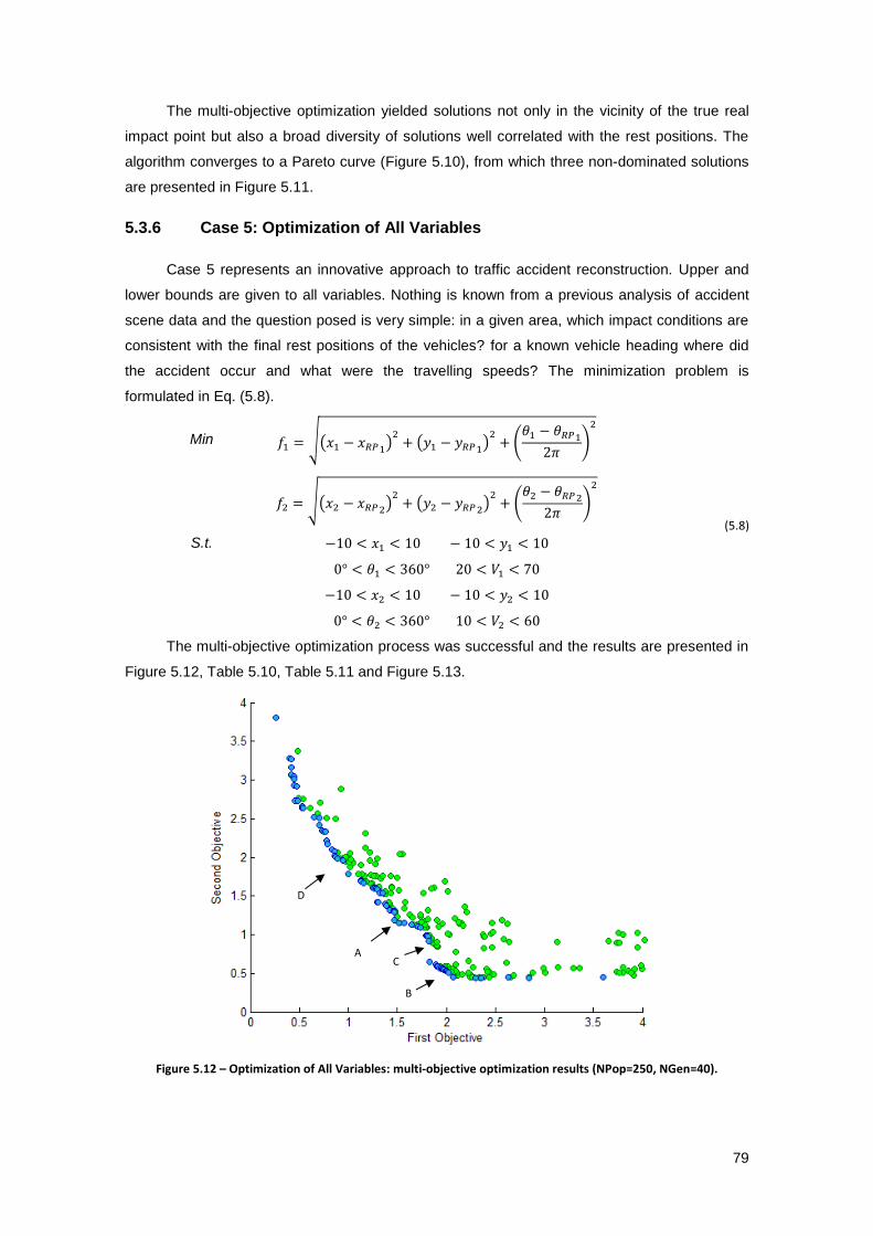
79

The multi-objective optimization yielded solutions not only in the vicinity of the true real

impact point but also a broad diversity of solutions well correlated with the rest positions. The

algorithm converges to a Pareto curve (Figure 5.10), from which three non-dominated solutions

are presented in Figure 5.11.

5.3.6 Case 5: Optimization of All Variables

Case 5 represents an innovative approach to traffic accident reconstruction. Upper and

lower bounds are given to all variables. Nothing is known from a previous analysis of accident

scene data and the question posed is very simple: in a given area, which impact conditions are

consistent with the final rest positions of the vehicles? for a known vehicle heading where did

the accident occur and what were the travelling speeds? The minimization problem is

formulated in Eq. (5.8).

Min √( ) ( )

(

)

(5.8)

√( ) ( )

(

)

S.t.

The multi-objective optimization process was successful and the results are presented in


Figure 5.12 – Optimization of All Variables: multi-objective optimization results (NPop=250, NGen=40).

B

C A

D

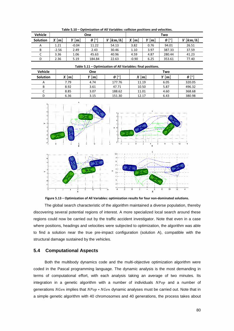
80

Table 5.10 – Optimization of All Variables: collision positions and velocities.

Vehicle One Two

Solution [ ] [ ] [ ] [ ] [ ] [ ] [ ] [ ]

A 1.21 -0.04 11.22 54.13 3.82 0.76 94.01 26.51

B -2.56 2.49 2.43 30.46 1.10 3.97 387.33 37.59

C 3.36 1.06 45.63 40.96 4.59 4.87 280.44 41.23

D 2.36 5.19 184.84 22.63 -0.90 6.25 353.61 77.40

Table 5.11 – Optimization of All Variables: final positions.

Vehicle One Two

Solution [ ] [ ] [ ] [ ] [ ] [ ]

A 7.79 4.74 177.76 11.19 6.05 320.05

B 8.92 3.61 47.71 10.50 5.87 496.32

C 8.85 3.07 188.62 11.01 4.60 368.68

D 6.36 3.15 151.30 12.17 6.43 380.98

Figure 5.13 – Optimization of All Variables: optimization results for four non-dominated solutions.

The global search characteristic of the algorithm maintained a diverse population, thereby

discovering several potential regions of interest. A more specialized local search around these

regions could now be carried out by the traffic accident investigator. Note that even in a case

where positions, headings and velocities were subjected to optimization, the algorithm was able

to find a solution near the true pre-impact configuration (solution A), compatible with the

structural damage sustained by the vehicles.

5.4 Computational Aspects

Both the multibody dynamics code and the multi-objective optimization algorithm were

coded in the Pascal programming language. The dynamic analysis is the most demanding in

terms of computational effort, with each analysis taking an average of two minutes. Its

integration in a genetic algorithm with a number of individuals and a number of

generations implies that dynamic analyses must be carried out. Note that in

a simple genetic algorithm with 40 chromosomes and 40 generations, the process takes about

81

53 hours to complete. Even though this might seem a major disadvantage of the method

proposed in the present dissertation, it can be overcome by recent advances such as parallel

processing. Furthermore, the major contribution of this dissertation is not the multibody

dynamics tool to simulate traffic accidents but rather the proposal of a new traffic accident

reconstruction method, by means of a multi-objective optimization routine which is, in itself,

applicable to any type of collision model. Its application to a momentum-impulse collision model

could greatly reduce the computational time associated with each analysis. Its applicability is

however limited, as momentum formulations cannot be applied to accidents involving rollovers,

pedestrians or models of two-wheeled vehicles.

83

6 Conclusions and Future Developments

6.1 Conclusions

In this dissertation, a computational tool to study a collision between two automobiles was

developed. Using multibody dynamics formulations, the three-dimensional motion of vehicles is

analyzed considering suspensions, road/tire interaction, contact detection and contact forces

through a methodology that uses superellipsoids to model the surfaces of the vehicles. The

multibody dynamics tool has traffic accident reconstruction as its main objective. Several case

studies were presented and compared with the outcomes of a widely used commercial accident

reconstruction software, PC-Crash, with satisfactory results.

The main goal of the present dissertation was to propose a new approach to traffic

accident reconstruction. It shows that using multibody dynamics formulations, good results can

be obtained regarding the collision of two motor vehicles but its highest contribution to the field

is the introduction of a new method to tackle the accident reconstruction problem by the use of

multi-objective optimization. Since a multi-objective optimization algorithm converges to a

population of non-dominated solutions, it constitutes a viable technique to determine a number

of trade-off near-optimal impact configurations that can then be compared by the traffic accident

investigator. The multi-objective optimization methodology was successfully applied to a real

traffic accident, showing that it can accurately determine several pre-impact configurations

consistent with the vehicle’s rest positions.

While the results presented in this dissertation may depend on the accuracy of the

multibody dynamics code developed to simulate the collision between two automobiles, the

multi-objective optimization process in itself was shown to be a viable new approach to traffic

accident reconstruction and is applicable to any kind of collision model. The results so far

indicate that multi-objective optimization can be a powerful tool when applied to traffic accident

reconstruction in which the process of trial and error normally used by investigators can be

replaced by a user independent approach that leads to reliable results.

In the first optimizations performed it was found that many of the generated solutions

were not admissible for the problem in question, either by not corresponding to a collision

course or by corresponding to a configuration in which the vehicles were overlapped. This

problem was dealt by the implementation of loop that only accepted solutions in which these

two situations did not occur. However, this may hinder the evolution process since these

solutions are a part of evolution. Consequently, and regarding the question of overlapped

solutions, a new operator can be developed that backs up the vehicles along their heading until

a configuration is reached in which they are no longer overlapped.

Furthermore, it was determined that even though the multi-objective optimization process

constitutes a powerful new tool in traffic accident reconstruction, its application to a multibody

dynamics code results in a very time consuming process. Its application to an impulse-

momentum collision model could either greatly reduce the computational time or, for the same

84

computational time, allow the use of much larger populations and generations. Note that small

populations may cause a weak performance of the algorithm as there may not be sufficient

individuals to cover the entire search space and, on the other hand, large populations increase

the computational effort, slowing the evolution process. On the other hand, this gain in

computational time would have to be paid with the loss of model complexity, since accidents

involving models of pedestrians or two-wheeled vehicles could not be reconstructed.

6.2 Future Developments

The implemented multi-objective optimization method was a non-dominated sorting

genetic algorithm, which was able to find several non-dominated solutions corresponding to

different possible pre-impact conditions. It has, however, been criticized due to the need to

specify a sharing parameter and its lack of elitism, i.e., it has not method to explicitly prevent the

loss of good solutions once they have been found. In addition, Zitzler, Deb & Lothar (2000)

shows that the use of elitism can improve the performance of the algorithm. The implementation

of a multi-objective optimization algorithm with elitism, such as NSGA-II, could not only increase

the performance of the optimization procedure but also uncover a larger set of solutions on the

true optimal Pareto front. Another option would be to use the highly competitive Direct

MultiSearch for its impressive ability to generate the whole Pareto front (Custodio, Madeira,

Vaz, & Vicente, 2011).

Another important development would be to integrate algorithms in a guided user

interface using the OpenGL graphic library for three-dimensional rendering of the results

(Zhang, Liu, & Zhang, 2010), allowing its use and validation by other investigators.

Nowadays, vehicles are becoming more similar to each other regarding their

crashworthiness and deformation behavior, so the application of finite element methods to

replicate the deformation and energy absorbed by the vehicles might become suitable. This

approach could provide a further improvement of traffic accident simulations.

Multibody dynamics formulations have proven their importance in the field of accident

reconstruction, namely in what concerns to pedestrian impacts and collisions involving

motorcyclists. Replacing the superellipsoid contact model used in this dissertation by one based

in polygonal mesh surfaces would enable the use of more complex vehicle surfaces and

detailed human models. An important feature to include in the human models would be the

automatic calculation of biomechanical indexes such as the Head Injury Criterion or the

Thoracic Trauma Index. Even though the Head Injury Criterion is relatively simple to calculate,

the Thoracic Trauma Index would require a detailed model. One possibility would be to use a

co-simulation procedure, already successfully applied to railway dynamics to model the

interaction between a multibody pantograph and a finite element model of a catenary (Antunes,

2012). In a co-simulation environment, multibody models of the human body could be used in

conjunction with finite element models of areas of interest such as the brain or cervical spine.

The problem dealt in the present dissertation is a member of the HEB category, i.e., it’s a

High-dimensional, Expensive (computationally), Black-box problem. One of the big hindrances

85

experienced with the integration of a detailed multibody dynamics simulation in a genetic

optimization routine was the resultant substantial computational time. One possible way of

tackling this problem without sacrificing model complexity would be to use metamodelling

techniques, which are becoming a popular approach to alleviate the computational burden of

complex optimization problems. The integration of a method such as response surfaces,

Taylor’s series or neural networks would eliminate the need to calculate every single objective

function value through a computationally expensive simulation model, resulting in higher

computational efficiency.

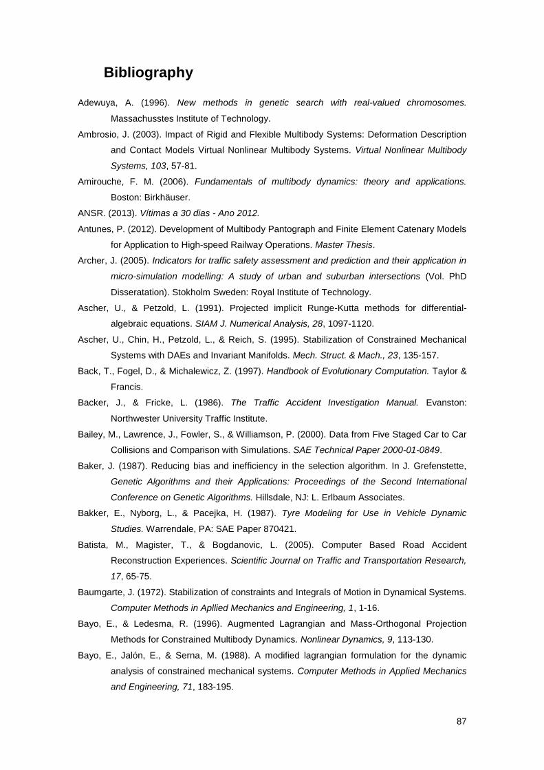
87

Bibliography

Adewuya, A. (1996). New methods in genetic search with real-valued chromosomes.

Massachusstes Institute of Technology.

Ambrosio, J. (2003). Impact of Rigid and Flexible Multibody Systems: Deformation Description

and Contact Models Virtual Nonlinear Multibody Systems. Virtual Nonlinear Multibody

Systems, 103, 57-81.

Amirouche, F. M. (2006). Fundamentals of multibody dynamics: theory and applications.

Boston: Birkhäuser.

ANSR. (2013). Vítimas a 30 dias - Ano 2012.

Antunes, P. (2012). Development of Multibody Pantograph and Finite Element Catenary Models

for Application to High-speed Railway Operations. Master Thesis.

Archer, J. (2005). Indicators for traffic safety assessment and prediction and their application in

micro-simulation modelling: A study of urban and suburban intersections (Vol. PhD

Disseratation). Stokholm Sweden: Royal Institute of Technology.

Ascher, U., & Petzold, L. (1991). Projected implicit Runge-Kutta methods for differential-

algebraic equations. SIAM J. Numerical Analysis, 28, 1097-1120.

Ascher, U., Chin, H., Petzold, L., & Reich, S. (1995). Stabilization of Constrained Mechanical

Systems with DAEs and Invariant Manifolds. Mech. Struct. & Mach., 23, 135-157.

Back, T., Fogel, D., & Michalewicz, Z. (1997). Handbook of Evolutionary Computation. Taylor &

Francis.

Backer, J., & Fricke, L. (1986). The Traffic Accident Investigation Manual. Evanston:

Northwester University Traffic Institute.

Bailey, M., Lawrence, J., Fowler, S., & Williamson, P. (2000). Data from Five Staged Car to Car

Collisions and Comparison with Simulations. SAE Technical Paper 2000-01-0849.

Baker, J. (1987). Reducing bias and inefficiency in the selection algorithm. In J. Grefenstette,

Genetic Algorithms and their Applications: Proceedings of the Second International

Conference on Genetic Algorithms. Hillsdale, NJ: L. Erlbaum Associates.

Bakker, E., Nyborg, L., & Pacejka, H. (1987). Tyre Modeling for Use in Vehicle Dynamic

Studies. Warrendale, PA: SAE Paper 870421.

Batista, M., Magister, T., & Bogdanovic, L. (2005). Computer Based Road Accident

Reconstruction Experiences. Scientific Journal on Traffic and Transportation Research,

17, 65-75.

Baumgarte, J. (1972). Stabilization of constraints and Integrals of Motion in Dynamical Systems.

Computer Methods in Apllied Mechanics and Engineering, 1, 1-16.

Bayo, E., & Ledesma, R. (1996). Augmented Lagrangian and Mass-Orthogonal Projection

Methods for Constrained Multibody Dynamics. Nonlinear Dynamics, 9, 113-130.

Bayo, E., Jalón, E., & Serna, M. (1988). A modified lagrangian formulation for the dynamic

analysis of constrained mechanical systems. Computer Methods in Applied Mechanics

and Engineering, 71, 183-195.

88

Bergen, G. (1999). Collision detection in interactive 3D computer animation. Eindhoven:

Technische Universiteit Eindhoven.

Bergen, G. (2004). Collison detection in interactive 3D environments. Amsterdam:

Elsevier/Morgan Kaufman.

Bhalerao, K., & Anderson, K. (2010). Modeling intermittent contact for flexible multibody

systems. Nonlinear Dynamics, 63-79.

Blickle, T., & Thiele, L. (1995). A Mathematical Analysis of Tournament Selection. Proceedings

of the Sixth International Conference on Genetic Algorithms, 9-16.

Bogdanovic, V., Milutinovic, N., Kostic, S., & Ruskic, N. (2012). Research Of The Influences of

Input Parameters On The Result Of Vehicles Collision Simulation. PROMET - Traffic &

Transportation, 24, 243-251.

Brach, R. (1983). Analysis of Planar Vehicle Collisions Using Equations of Impulse and

Momentum. Accident Analysis & Prevention, 15, 115-120.

Brach, R. (1991). Mechanical impact dynamics: rigid body collisions. New York: John Wiley &

Sons.

Brach, R. (1994). Uncertainty in Accident Reconstruction Calculations. SAE Technical Paper

940722.

Brach, R., & Brach, R. (1987). A Review of Impact Models for Vehicle Collision. SAE Technical

Paper 870048.

Brach, R., & Brach, R. (2000). Modeling Combined Braking and Steering Tire Forces.

Warrendale: SAE Paper 2000-01-0357.

Broughton, J., Knowles, J., Brandstatter, C., Yannis, G., Evgenikos, P., Papantoniou, P., . . .

Sanmartin, J. (2011). Traffic Safety Basic Facts 2011. European Road Safety

Observatory.

Buck, U., Naether, S., Braun, M., Bolliger, S., Friederich, H., Jackowski, C., . . . Thali, M. (2007).

Application of 3D documentation and geometric reconstruction methods in traffic

accident analysis: With high resolution surface scanning, radiological MSCT/MRI

scanning and real data based animation. Forensic Science International, 170, 20-28.

Buck, U., Naether, S., Rass, B., Jackowski, C., & Thali, M. (2013). Accident or homicide –

Virtual crime scene reconstruction using 3D methods. Forsensic Science International,

225, 75-84.

Campbell, K. (1974). Energy Basis for Collision Severity. SAE Technical Paper 740565.

Chang, C., & Nikravesh, P. (1985). Optimal Design of Mechanical Systems with Constraint

Violation Stabilization Method. J. of Mechanisms, Transmissions and Automation in

Design, 107, 493-498.

Chapra, S., & Canale, R. (2009). Numerical Methods for Engineers. MacGraw-Hill.

Charles, A., & Cooper, W. (1961). Management models and industrial applications of linear

programming. John Wiley: New York.

Chen, Y., & Yang, J. (2009). Reconstruction of a passenger carto-child pedestrian accident.

Journal of Hunan University (Natural Science), 36, 35-40.

89

Chidester, A., Hinch, J., Mercer, T., & Schultz, K. (1999). Recording Automotive Crash Event

Data. Proceedings of the International Symposium on Transportation Recorders, 3-5.

Cieniawski, S. (1993). An investigation of the ability of genetic algorithms to generate the

tradeoff curve of a multi-objective groundwater monitoring problem. Master Thesis.

Cliff, W., & Montgomery, D. (1996). Validation of PC-Crash - A Momentum-Based Accident

Reconstruction Program. SAE Technical Paper 960885.

Cliff, W., & Moser, A. (2001). Reconstruction of twenty staged collisions with PC-Crash's

optimizer. SAE Technical Paper 2001-01-0507.

Cooner, S., & Balke, K. (2000). Use of photogrammetry for investigation of traffic incident

scenes. Texas Transportation Institute.

Corne, D., Knowles, J., & Oates, M. (2000). The Pareto enveloped-based selection algorithm for

multiobjective optimiation. Sixth International Conference on Parallel Solving from

nature, 839-848.

Custodio, A., Madeira, J., Vaz, A., & Vicente, L. (2011). Direct Multisearch for MultiObjective

Optimization. SIAM Journal on Optimization, 21, 1109-1140.

Darwin, C. (1859). The origin of species by menas of natural selection. John Murray.

Datentechnik , S. (2011). PC-Crash Technical Manual Version 9.0. Linz, Austrian: Mea

Forensic.

Datentechnik, S. (2009). PC-Rect A Photograph Rectification Program. Linz, Austria: Macinnis

Engineering Associates.

Datentechnik, S. (2010). PC-Crash A simulation Program for Vehicle Accidents Operating

Manual 9.0. Linz, Austria: Mea Forensic.

David, R. (2007). A Generalized Two-Dimensional Model to Reconstruct the Impact Phase in

Automobile Collisions. Master Thesis in Mechanical Engineering.

Day, T. (1999). An Overview of the EDSMAC4 Collision Simulation Model. SAE Technical

Paper 1999-0.-0102.

Day, T., & Hargens, R. (1989). Application and Misapplication of Computer Programs for

Accident Reconstruction. SAE Technical Paper 890738.

Day, T., & Hargens, R. (1990). Further Validation of EDSMAC Using the RICSAC Staged

Collisions. SAE Technical Paper 900102.

De Jong, K. (1975). Analysis of the behaviour of a class of genetic adapttive systems. PhD

Dissertation, University of Michigan.

Deb, Agrawal, S., Pratap, A., & Meyarivan, T. (2000). A fast elitist non-dominated sorting

genetic algorithm for multiobjective optimization: NSGA II. Sixth International

Conference on Parallel Solving from Nature, VI, 849-858.

Deb, K. (2001). Multi-Objective Optimization using Evolutionary Algorithms. Wiley.

Deb, K., & Agrawal, R. (1995). Simulated binary crossover for continuous search space.

Complex Systems, 9, 115-148.

Deb, K., & Deb, D. (2012). Analyzing Mutation Schemes for Real-Parameter Genetic

Algorithms. Kanpur Genetic Algorithms Laboratory Report Number 2012016.

90

Deb, K., Reddy, A., & Singh, G. (2003). Optimal scheduling of casting sequence using genetic

algorithms. Journal of Materials and Manufacturing Processes, 18, 409-432.

Dias, J., & Paulino, T. (2010). Computational Models for Helmet Use Assessment in Motorcycle

Accidents. 4th International Conference on ESAR "Expert Symposium on Accident

Research".

Dias, J., Portal, R., & Paulino, T. (2012). Forensic Injury Biomechanics Methodologies Applied

To Traffic Accident Reconstruction. ESB2012: 18th Congress of the European Society

of Biomechanics, Presentation 1788.

Djerassi, S. (2009). Collision with friction; Part A: Newton's hypothesis. Multibody System

Dynamics, 21, 37-54.

Eberly, D. (2007). 3D game engine design : a practical approach to real-time computer

graphics. Boston: Elsevier/Morgan Kaufmann.

Ehrgott, M. (2000). Multicriteria Optimization. Berlin: Springer.

Eos Systems Inc. (2012). PhotoModeler 2012 User Manual.

Eshelman, L., & Shaffer, J. (1993). Real-coded genetic algorithms and interval-schemata. In L.

Whitley, Foundations of genetic algorithms 2 (pp. 187-202). Morgan Kaufman.

Euro NCAP. (2012). Frontal Impact Testing Protocol (Version 6.0 ed.).

European Commision. (2010). Towards a European road safety area: policy orientations on

road safety 2011-2020. Brussels.

European Commission - Directorate General Energy and Transport. (2012). Road safety

evolution in EU Mars 2012. European Commission.

European Commission - Directorate General for Mobility and Transport. (2013). EU road

fatalities March 2013. European Commission.

European Commission. (2001). European transport policy for 2010: time to decide. Brussels.

European Road Safety Observatory. (2011). Annual Statistical Report 2011.

European Road Safety Observatory. (2012). Traffic Safety Basic Facts 2012 Main Figures.

Directorate-General for Mobility & Transport.

European Transport Safety Council. (2012). 2010 Road Safety Target Outcome: 100,000 fewer

deaths since 2001 5th Road Safety PIN Report.

European Transport Safety Council. (2012). A Challenging Start Towards the EU 2020 Road

Safety Target: 6th Road Safety PIN Report.

Fan, Y., Xu, H., & Liu, X. (2008). Simulation on Kinematics Law of Pedestrian in

Vehicle/Pedestrian Contacting Phase. The 9th International Conference for Young

Computer Scientists, 731-736.

Fay, R., Robinette, R., Scott, J., & Fay, P. (2001). PC-Crash and HVE, an Overview of

Similarities and Differences. SAE Technical Paper 2001-01-0505.

Fenton, S., & Kerr, R. (1997). Accident Scene Diagramming Using New Photogrammetric

Technique. SAE Technical Paper 970944.

Ferreira, A. (2012). Evaluation of whiplash injuries in victims from road accidents in Portugal. (I.

T. Lison, Ed.) Lisbon: Master Thesis in Biomedical Engineering.

91

Fittanto, D., Ruhl, R., Southcombe, E., Burg, H., & Burg, J. (2002). Overview of CARAT-4 a

Multi-body Simulation and Collision Modeling Program. SAE Technical Paper 2002-01-

1566.

Flickinger, D., & Bowling, A. (2010). Simultaneous oblique impacts and contacts in multibody

systems with friction. Multibody System Dynamics, 23, 249-261.

Flores, P., & Ambrosio, J. (2010). On the contact detection for contact-impact analysis in

multibody systems. Multibody System Dynamics, 24, 103-122.

Flores, P., Ambrósio, J., Claro, J., & Lankarani, H. (2008). Kinematics and dynamics of

multibody systems with imperfect joints : models and case studies. Berlim: Springer.

Flores, P., Machado, M., Seabra, E., & Silva, M. (2011). A Parametric Study on the Baumgarte

Stbilization Method for Forward Dynamics of Constrained Multibody Systems. Journal of

Computational and Nonlinear Dynamics, 6.

Flores, P., Machado, M., Silva, M., & Martins, J. (2011). On the continuous contact force models

for soft materials in multibody dynamics. Multibody System Dynamics, 25, 357-375.

Fonseca, C., & Fleming, P. (1995). An overview of evolutionary algorithms in multi-objective

optimization. Evolutionary Computation Journaç, 3, 1-16.

Fonseca, F., & Fleming, P. (1993). Genetic algorithms for multiobjective optimization:

Formulation, discussion and generalization. Proceedings of the Fifth International

Conference on Genetic Algorithms, 416-423.

Fricke, L. (1990). Traffic Accident Reconstruction. Northwestern University Center for Public

Safety.

Gabler, H., & Roston, T. (2003). Estimating Crash Severity: Can Event Data Recorders Replace

Crash Reconstruction? Proceedings of the Eighteenth International Conference on

Enhanced Safety of Vehicles.

Gabler, H., Hampton, C., & Hinch, J. (2004). Crash Severity: A Comparison of Event Data

Recorder Measurements with Accident Reconstruction Estimates. SAE Technical Paper

2004-01-1194.

Galileo, G. (1692). Dialogue on the Two Chief World Systems. Florence.

Gear, C. (1971). Numerical Initial Value Problems in Ordinary Differential Equations. Englewood

Cliffs, New Jersey: Prentice-Hall.

Gear, C. W. (1981). The Simultaneous Numerical Simulation of Differential-Algebraic Equations.

IEEE Translations on Circuit Theory, 18, 88-95.

Gear, C., & Petzold, L. (1984). ODE methods for the solutions of differential/algebraic

equations. SIAM Journal Numerical Analysis, 21, 716-728.

Geigl, B., Hoschpof, H., Steffan, H., & Moser, A. (2003). Reconstruction of occupant kinematics

and kinetics for real world accidents. International Journal of Crashworthiness, 8, 17-27.

German, A., Comeau, J.-L., Monk, B., McClafferty, K., Tiessen, P., & Chan, J. (2001). The Use

of Event Data Recorders in the Analysis of Real-World Crashes. Proceedings of the

Canadian Multidisciplinary Road Safety Conference XII.

92

Gilardi, G., & Sharf, I. (2002). Literature survey of contact dynamics modeling. Mech. Mach.

Theory, 37, 1213-1239.

Gim, G., & Nikravesh, P. (1990). An Analytical Model of Pneumatic Tire for Vehicle Dynamic

Simulations. International Journal of Vehicle Design, 11, 589-618.

Goldberg, D. (1989). Genetic algorithms in search, optimization and machine learning. Addison-

Wesley.

Goldberg, D., & Richardson, J. (1987). Genetic algorithms with sharing for multimodal function

optimization. Proceedings of the First International Conference on Genetic Algorithms

and Their Applications, 41-49.

Goldberg, D., & Segrest, P. (1985). Finite markov chain analysis of genetic algorithms. Genetic

Algorithms and Their Applications: Proceedings of the First International Conference on

Genetic Algorithms (pp. 1-8). Lawrence Erlbaum.

Goldsmith, W. (1960). Impact: the theory and physical behaviour colliding solids. London:

Edward Arnold Ltd.

Goldstein, H. (1980). Classical Mechanics, 2nd Edition. Reading, MA: Addison-Wesley.

Gonçalves, J. (2002). Rigid and Flexible Multibody Systems Optimization for Vehicle Dynamics.

Lisbon: PhD Thesis, Instituto Superior Tecnico, Technical University of Lisbon.

Guan-quan, L., Hong-guo, L., Hong-fei, L., & Li-fang, W. (2002). Two-eyes-visual method to

reconstruct measuring point on traffic accident scene. Journal of Highway and

Transportation Research and Development, 2, 94-96.

Haimes, Y., Lasdon, L., & Wismer, D. (1971). On a biocriterion formulation of the problems of

integrated system identification and system optimization. IEEE Transactions on

Systems, 1, 296-297.

Haug, E. J. (1989). Computer Aided Kinematics and Dynamics of Mechanical Systems.

Needham Heights, Massachusetts: Allyn and Bacon.

He, K., Dong, S., & Zhou, Z. (2007). Multigrid contact detection method. Physical Review, 75.

Hertz, H. (1896). On the contact of rigid elastic solids - on the contact of rigid elastic solids and

on hardness. London, England: Macmillan and Co. Ltd.

Hippmann, G. (2004). An algorithm for compliant contact between complexely shaped bodies.

Multibody System Dynamics, 12, 345-362.

Hirschberg, Rill, & Weinfurter. (2007). Tire model TMeasy. Vehicle System Dynamics, 45, 101-

119.

Holland, J. (1975). Adaptation in natural and artificial systems. Ann Arbor: MIT Press.

Hollowell, W., Gabler, H., Stucki, S., Stephen, S., & Hackney, J. (1999). Updated Review of

Potential Test Procedures For FNVSS No. 208. NHTSA.

Horn, J., & Nafpliotis, N. (1993). Multiobjective optimization using the niched Pareto genetic

algorithm. IlliGAL Report 93005.

Horn, J., Nafpliotis, N., & Goldberg, D. (1994). A niched Pareto genetic algorithm for

multiobjective optimization. Proceedings of the First IEEE Conference on Evolutionary

Algorithms, 1, 82-87.

93

Hunt, K., & Crossley, F. (1975). Coefficient of Restitution Interpreted as Damping in

Vibroimpact. Journal of Applied Mechanics, 42, 440-445.

Jaklic, A., & Leonardis, A. (2000). Segmentation and recovery of superquadrics. Boston: Klwer

Academic Publishers.

Jalón, J., & Bayo, E. (1994). Kinematic and dynamic simulation of multibody systems: the real-

time challenge. New York: Springer-Verlag.

Jones, G., Brown, R., Clark, D., Willet, P., & Glen, R. (1993). Searching databases of two-

dimensional and three-dimensional chemical structures using genetic algorithms.

Genetic Algorithms: Proceedings of the Fifth International Conference (pp. 597-602).

San Mateo, CA: Morgan Kaufmann.

Kepler, J. (1609). AStronomia Nova. Graz.

Khulief, Y., & Shabana, A. (1986). Dynamic analysis of constrained system of rigid and flexible

bodies with intermittent motion. Journal of Mechanisms, Transmissions and Automation,

108, 38-45.

Kim, S., & Vanderploeg, M. (1986). QR Decomposition for State Space Representation of

Constrained Mehcanical Dynamic System. Journal of Mech. Trans. and Automation,

108, 176-182.

King's County Chronicle. (1869, 09 01). Appalling Accident: Sudden Death of the Hon. Mrs.

Ward.

Knowles, J., & Corne, D. (2000). Approximating the nondominated front using the Pareto

archive evolution strategy. Evolutionary Computation, 2, 149-172.

Koza, J. (1992). Genetic Programming: on the programming of computers by means of natural

selection. MIT Press.

Kudlich, H. (1966). Beitrag zur Mechanik des Kraftfahreug-Verkehrsunfalls. TU-Wien:

Dissertation.

Lagrange, J. (1788). Mécanique Analytique. Paris: L'Académie Royal des Sciences.

Lankarani, H. (1988). Canonical equations of motion and estimation of parameters in the

analysis of impact problems, PhD Disseration. Tucson Arizona: University of Arizona.

Lankarani, H., & Nikravesh, P. (1990). A Contact Force Model With Hysteresis Damping for

Impact Analysis of Multibody Systems. Journal of Mechanical Design, 112, 369-376.

Lankarani, H., & Nikravesh, P. (1994). Continuous contact force models for impact analysis in

multibody systems. Nonlinear Dynamics, 5, 193-207.

Lawrence, J., Wilkinson, C., King, D., Heinrichs, B., & Sigmund, G. (2003). The Accuracy and

Sensitivity of Event Data Recorders in Low Speed Collisions. SAE Technical Paper 01-

0679.

Lenard, J., Hurley, B., & Thomas, P. (2000). The statistical accuracy of Delta-V in systematic

field accident studies. Proceedings of IMechE Conference 'VS 2000'.

Leonard, M., Croteau, J., Werner, S., Tuskan, S., & Habberstad, J. (2000). HVE EDSMAC4

Trailer Model Simulation Comparison with Crash Test Data. SAE Technical Paper

2000-01-0468.

94

Li, F., & Yang, K. (2010). A study of head–brain injuries in car-to-pedestrian crashes with

reconstructions using in-depth accident data in China. International Journal of

Crashworthiness, 15, 117-124.

Machado, M., Flores, P., Claro, J., Ambrosio, J., Silva, M., Completo, A., & Lankarani, H.

(2010). Development of a planar multibody model of the human knee joint. Nonlinear

Dynamics, 60, 459-478.

Machado, M., Moreira, P., Flores, P., & Lankarani, H. (2012). Compliant contact force models in

multibody dynamics: Evolution of the Hertz contact theory. Mechanism and Machine

Theory, 53, 99-121.

Madeira, J. F. (2004). Optimização Multi-Objectivo da Topologia de Estruturas Com Algoritmos

Genéticos. (U. o. IST, Ed.) Lisbon: PhD Dissertation.

Martins, G., & Neto, M. (2008). Técnicas de otimização aplicadas ao problema de

reconstituição de acidentes de veículos. Inteligência Computacional Aplicada, 1.

McHenry, R. (1968). An analysis of the dynamics of automobiles during simultaneous cornering

and ride motions, in handling of vehicles under emergency conditions. Proceedings of

the Instrumental Mechanical Engineers, 13, pp. 28-48.

McHenry, R. (1971). Development of a Computer Program to Aid in the Investigation of

Highway Accidents. (C. Corporation, Ed.) Cal Report No. V3-2979-V-1.

McHenry, R. (1975). A Comparison of Results Obtained With Different Analytical Techniques for

Reconstruction of Higway Accidents. SAE Technical Paper 750893.

McHenry, R. (1975). The CRASH Program - A Simplified Collision Reconstruction Program.

Proceedings of the Motor Vehicle Collision Investigation Symposium.

McHenry, R. (1976). Computer Aids for Accident Investigation. SAE Technical Paper 760776.

McHenry, R., & McHenry, B. (1997). Effects of Restitution in the Application of Crush

Coefficients. SAE Technical Paper 970960.

McHenry, R., Segal, D., Lynch, D., & Henderson, P. (1973). Mathmatical Reconstruction of

Highway Accidents. CAL Report No. ZM-5096-V-1.

Michalewicz, Z. (1994). Genetic Algorithms + Data Structures = Evolution Programs. New York:

Springer-Verlag.

Mitis, F., & Sethi, D. (2013). European Facts and Global Status Report on Road Safety 2012.

World Health Organization Regional Office for Europe.

Moser, A., & Steffan, H. (1998). Automatic Optimization of Pre-Impact Parameters Using Post

Impact Trajectories and Rest Positions. SAE Technical Paper 980373.

Moser, A., Hoschpof, H., Steffan, H., & Kasanicky, G. (2000). Validation of the PC-Crash

Pedestrian Model. SAE Technical Paper 2000-01-0847.

Moser, A., Steffan, H., & Kasanicky, G. (1999). The Pedestrian Model in PC-Crash - The

Introduction of a Multi Body System and its Validation. SAE Technical Paper 1999-01-

0445.

95

Moser, A., Steffan, H., Spek, A., & Makkinga, W. (2003). Application of the Monte Carlo

Methods for Stability Analysis within the Accident Reconstruction Software PC-CRASH.

SAE Technical Paper 2003-01-0488.

Mousseau, C., & Hulbert, G. (1996). An Efficient Tire Model for the Analysis of Spindle Forces

Produced by a Tire Impacting Large Obstacles. Computational Methods Applied

Mechanical Engineering, 135, 15-34.

Musseau, C., Darnell, I., & Hulbert G. (1997). An Efficient Three-Dimensional Tire Model for

Vehicle Dynamics Simulation. Mechanics of Structures and Machines, 25, 1-19.

Najafabadi, S., Kovecses, J., & Angeles, J. (2008). Impacts in multibody systems: modeling and

experiments. Multibody System Dynamics, 20, 163-176.

Neto, M., & Ambrósio, J. (2003). Stabilization Methods for the Integration of DAE in the

Presence of Redundant Constraints. Multibody System Dynamics, 10, 81-105.

Newton, I. (1687). Philosophiae Naturalis Principia Mathematica. London: Royal Society.

Niehoff, P., Hampton, G., Brophy, J., Chidester, C., Hinch, J., & Ragland, C. (2005). Evaluation

of event data recorders in full systems crash tests. Proceedings of the 19th International

Technical Conference on the Enhanced Safety of Vehicles (ESV).

Nikravesh, P. (1984). Some Methods for Dynamic Analysis of Constrained Mechanical Systems:

A Survey. In E. Haug, Computer-Aided Analysis and Optimization of Mechanical

System Dynamics (pp. 351-368). Berlin: Springer-Verlag.

Nikravesh, P. (1988). Computer Aided Analysis of Mechanical Systems. Englewood Cliffs, New

Jersey: Prentice Hall.

Nikravesh, P. (1990). Systematic reduction of multibody equations of motion to a minimal set.

International Journal of Nonlinear Mechanics, 25, 143-151.

Nolan, J., Preuss, C., Jones, S., & O'Neill, B. (1998). An update on the relationships between

computed delta Vs ans impact speeds for offset crash tests. Proceedings of the 16th

International Technical Conference on Enhanced Safety of Vehicles, 2, 1234-1241.

O'Riordain, K., Thomas, P., Phillips, J., & Gilchrist, M. (2003). Reconstruction of real world head

injury accidents resulting from falls using multibody dynamics. Clinical Biomechanics,

18, 590-600.

Orlandea, N., Chace, M., & Calahan, D. (1977). A sparsity-oriented approach to the dynamic

analysis and design of mechanical systems , Parts I and II. Trans. ASME Journal

Engineering for Insdustry, 99, 773-784.

Osykza, A., & Kundu, S. (1997). A new method to solve generalized multicriteria optimization

problems using the simple genetic algorithm. Strctural Optimization, 10, 246-253.

Pacejka, H., & Sharp, R. (1991). Shear Force development by Pneumatic Tires in Steady State

Conditions: A Review of Modeling Aspects. Vehicle System Dynamics, 20, 121-176.

Pareto, V. (1896). Cours d'economie politique. Laussane: F. Rouge.

Petzold, L. (1981). An e•cient numerical method for solving stiff and non-stiff systems of

ordinary differential equations. SIAM Journal on Numerical Analisys, 18, 455-479.

96

Pombo, J. (2004). A Multibody Methodology for Railway Dynamics Applications. Lisbon: PhD

Thesis, Instituto Superior Tecnico, Technical University of Lisbon.

Pombo, J., & Ambrósio, J. (2007). A new wheel-rail contact model for railway dynamics. Vehicle

System Dynamics, 45, 165-189.

Portal, R. (2006). Modelos de Corpos Múltiplos para a Reconstituição de Acidentes Rodoviários

(Vol. MSc). Lisbon: Technical University of Lisbon.

Portal, R. (2013). Development of Vehicle Collision Methodologies for Application to Accident

Reconstruction. Lisbon: Doctoral Thesis in Mechanical Engineering.

Portal, R., Dias, J., & Sousa, L. (2009). Contact detection between convex superquadric

surfaces on multibody dynamics. Proceedings of the Multibody Dynamics 2009.

Warsaw, Poland: ECCOMAS Thematic Conference.

Portal, R., Dias, J., & Sousa, L. (2010). Contact Detection Between Convex Superquadric

Surfaces. Archive of Mechanical Engineering, LVII, 165-186.

Potra, F. (1995). Runge-Kutta Integrators for Multibody Dynamics. Mechanics of Structures and

Machines, 23, 181-197.

Radcliff, N. (1991). Forma analysis and random respectful recombination. Procedings of the 4th

International Conference on Genetic Algorithms: Morgan Kauffman.

Rovidz, A., & Melegh, G. (2003). Modelling of road vehicle body deformation using EES values

detection. 2003 IEEE International Symposium on Intelligent Signal Processing, 149-

154.

Rudolph, G. (2011). Evolutionary search under partially ordered fitness sets. Proceedings of the

International Symposium on Information Science Innovations in Engineering of Natural

and Artificial Intelligent Systems (pp. 818-822). ISI 2001.

Sansone, R., & Sansone, L. (2010). Road Rage What’s Driving It? Psychiatry (Edgmont), 7, 14-

18.

Schaffer, J., & Grefenstette, J. (1985). Multi-objective learning via genetic algorithms.

Proceedings of the Ninth International Joint Conference on Artificial Inteligence (pp.

593-595). Morgan Kaufmann.

Schmitt, K.-U., Niederer, P., Muser, M., & Walz, F. (2007). Trauma Biomechanics: Accidental

injury in traffic and sports. Springer.

Segel, L. (1956). Theoretical prediction and experimental substantiation of the response of the

automobile to steering control, in research in automobile stability and control and in tyre

performance. Proceedings of the Instrumental Mechanics Engineers, 7, pp. 310-330.

Seiffert, U., & Wech, L. (2003). Automotive Safety Handbook. Warrendale, PA: SAE

International.

Shaffer, J. (1995). Multiple objective optimization with vector evaluated genetec algorithms.

Vanderbilt University: PhD Thesis.

Shampine, L., & Gordon, M. (1975). Computer Solution of Ordinary Differential Equations: The

Initial Value Problem. San Francisco: Freeman.

97

Siegmund, G., King, D., & Montgomery, D. (1996). Using Barrier Impact Data to Determine

Speed Change in Aligned, Low-Speed, Vehicle-to-Vehicle Collisions. SAE Technical

Paper 960887.

Silva, M. (2003). Human Motion Analysis Using Multibody Dynamics and Optimization Tools.

Lisbon: PhD Thesis, Instituto Superior Tecnico, Technical University of Lisbon.

Slibar, A. (1966). Die mechanischen Grundsätze des Stoßvorganges freier und geführter Körper

und ihre Anwendung auf den Stoßvorgang von Fahrzeugen. Archiv für Unfallforschung.

Smith, G. (1994). Conservation of Momentum Analysis of Two-Dimensional Colliding Bodies,

With or Without Trailers. SAE Technical Paper 940566.

Smith, R., Noga, A., & Thomas, J. (1982). Accuracy and Sensitivity of Crash. Washington DC:

US Department of Transportation.

Solomon, P. (1974). The Simulation Model of Automobile Collisions (SMAC) Operator's Manual.

NHTSA Accident Investigation Division.

Spears, W. (1998). The role of mutation and recombination in evolutionary algorithms. Fairfax:

George Mason University.

Spit, H. (2000). Evaluation of PC-Crash: as a tool for professional traffic accident. Delft: TNO

Automotive.

Spit, H. (2002). MC-Crash Probability distributions in traffic accident analysis. Master Thesis.

Srinivas, N., & Deb, K. (1994). Multiobjective optimization using nondominated sorting in genetic

algorithms. Evolutionary Computation, 2, 221-248.

Steffan, H., Geigl, B., & Moser, A. (1999). A New Approach to Occupant Simulation Through the

Coupling of PC-Crash and MADYMO. SAE Technical Paper 1999-01-0444.

Steffan, H., Moser, A., Spek, A., & Makkinga, W. (2007). Collision optimizer and Monte Carlo

methods in impact calculation. EVU-Annual meeting 2007.

Stucki, S., & Fessahale, O. (1998). Comparison of Measured Velocity Change in Frontal Crash

Tests to NASS Computed Velocity Change. SAE Technical Paper 980649.

Subke, J., Wehner, H., Wehner, D., & Szczepaniak, S. (2000). Streifenlichttopometrie (SLT): a

new method for the three-dimensional photorealistic forensic documentation in colour.

Forensic Science International, 113, 289-295.

TASS. (2010). MADYMO Reference Manual Release 7.2.

Teixeira, P. (2012). Risk factors for pedestrian injuries in Portugal. (I. T. Lisbon, Ed.) Lisbon:

Masther Thesis in Biomedical Engineering.

Thali, M., Braun, M., & Dirnhofer, R. (2003). Optical 3D surface digitizing in forensic medicine:

3D documentation of skin and bone injuries. Forensic Science International, 137, 203-

208.

Threlfall, D. (1978). The inclusion of Coulomb friction in mechanisms programs with particular

reference to DRAM au programme DRAM. Mechanism and Machine Theory, 13, 475-

483.

Tomasch, E. (2004). Accident Reconstruction Guidelines. Austria: Pan-European Co-ordinated

Accident and Injury Databases.

98

Tsongos, N. (1986). Crash 3 Technical Manual. US Department of Transportation.

Tumbas, N., & Smith, R. (1988). Measurement Protocol for Quantifying Vehicle Damage from

an Energy Basis Point of View. SAE Technical Paper 880072.

Tumbas, N., Gilberg, A., & Fricke, L. (1988). Minimum Guidelines for Efficiently Acquiring or

Preserving Basic Information in a Motor Vehicle Accident. SAE Technical Paper

880067.

Ueyama, M., Ogawa, S., Chikasue, H., & Muramatu, K. (1998). Relationship Between Driving

Behaviour and Traffic Accidents - Accident Data Recorder and Driving Monitor

Recorder. 16th International Technical Conference on the Enhanced Safety of Vehicles,

402-409.

UN General Assembly. (2010). 64/255 Improving global road safety. Resolution adopted by the

General Assembly.

United Nations. (2011). Global Plan for the Decade of Action for Road Safety 2011-2020.

Veldhuizen, D. (1999). Multiobjective Evolutionary Algorithms: Classifications, Analyses and

New Inovations. Dayton, Ohio: Air Force Institute of Technology.

Vezin, P., & Verriest, J. (2005). Development of a set of numerical human models for safety.

Proceedings of the 19th International Technical Conference on the Enhanced Safety of

Vehicles (ESV), 6-9.

Warner, C., Smith, G., James, M., & Germane, G. (1983). Friction Applications in Accident

Reconstruction. Warrendale: SAE Paper 830612.

Wehage, R., & Haug, E. (1982). Generalized Coordinate Partitioning for Dimension Reduction

in Analysis of Constrained Dynamic Systems. Journal of Mechanical Design, 104, 247-

255.

Wellmann, C., Lillie, C., & Wriggers, P. (2008). A contact detection algorithm for superellipsoids

based on the comon normal concept. Engineering Computations, 25, 432-442.

Whitley, D. (1989). The genitor and selection pressure: Why rank-based allocation of

reproductive trials is best. Proceedings of the Third International Conference on Genetic

Algorithms, 116-121.

Wienke, D., Lucasius, C., & Kateman, G. (1992). Multicriteria target vector optimization of

analytical procedures using a genetic algorithm. Part I. Theory, numerical simulations

and application to atomic emission spectroscopy. Analytica Chimica Acta, 265, 211-

225.

Wilson, P., & Macleod, M. (1993). Low implementation cost IIR digital filter design using genetic

algorithms. IEE/IEEE Workshop on Natural Algorithms in Signal Processing, 1, 41-48.

Wolley, R. (1985). The “IMPAC” Computer Program for Accident Reconstruction. SAE Technical

Paper 850254.

Wolley, R. (1987). The “IMPAC” Program for Collision Analysis. SAE Technical Paper 870046.

Woolley, R., & Warner, C. (1986). An Overview of Selected Computer Programs for Automotive

Accident Reconstruction. Transportation Research Record: Journal of the

Transportation Research Board, 1068, 18-33.

99

World Health Organization. (2013). Global Status Report on Road Safety 2013: Supporting a

Decade of Action.

Xianghai, C., Xianlong, J., Xiaoyun, Z., & Xinyi, H. (2011). The application for skull injury in

vehicle–pedestrian accident. International Journal of Crashworthiness, 16, 11-24.

Xinguang, D., Xianlong, J., Xiaoyun, Z., Jie, S., & Xinyi, H. (2009). Geometry features

measurement of traffic accident for reconstruction based on close-range

photogrammetry. Advances in Engineering Software, 40, 497-505.

Yang, J. (2003). Pedestrain head protection from car impacts. International Journal of Vehicle

Design, 32, 16-27.

Yen, J., & Petzold, L. (1998). An Efficient Newton-Type Iteration for the Numerical Solution of

Highly Oscillatory Constrained Multibody Dynamic Systems. SIAM Journal on Scientific

Computing, 19, 1513-1534.

York, A., & Day, T. (1999). The DyMesh Method for Three-Dimensional Multi-Vehicle Collision

Simulation. SAE Technical Paper 1999-01-0104.

Yukai, L., Xianlong, J., & Xinyi, H. (2005). Application of digital photogrammetry in accident

reconstruction. Journal of Computer-Aided Design & Computer Graphics, 17, 2318-

2322.

Zadeh, L. (1963). Optimality and non-scalar-valued performance criteria. IEEE Transactions on

Automatic Control, 8, 59-60.

Zhang, S., Liu, H., & Zhang, S. (2010). Researching on Simulation of Traffic Accidents Scene

by OpenGL. 10th IEEE International Conference on Computer and Information

Technology (CIT 2010), 1566-1570.

Zhang, X., Jin, X., & Guo, L. (2006). Improvement Design of the Auto-Body Oriented to the

Virtual Reconstruction Results of the Traffic Accident. Proceedings of the 16th

International Conference on Artificial Reality and Telexistence--Workshops, 180-183.

Zhang, X.-y., Jin, X.-l., Qi, W.-g., & Guo, Y.-z. (2008). Vehicle crash accident reconstruction

based on the analysis 3D deformation of the auto-body. Advances in Engineering

Software, 39, 459-465.

Zitzler, E., & Thiele, L. (1998). Multiobjective optimization using evolutionary algoriths - a

comparative study. Parallel Problem Solving from Nature, V, 292-301.

Zitzler, E., Deb, K., & Lothar, T. (2000). Comparison of Multiobjective Evolutionary Algorithms:

Empirical Results. Evolutionary Computation, 8, 173-195.

Zweep, C., Kellendonk, G., Leneman, F., Lemmen, P., & Bronckers, F. (2003). Numerical fleet

sutdies 2002-2003. Delft: TNO Automotive.

Simulation and Multi-Objective Optimization of Road Traffic … · Dame pelo livro de contacto que...

Documents

Transcript of Simulation and Multi-Objective Optimization of Road Traffic … · Dame pelo livro de contacto que...