Final Technical Report

Simulation and Modeling of Wood Dust Combustion in Cyclone Burners Prepared by: Stephen M. de Bruyn Kops and Philip C. Malte Energy and Environmental Combustion Laboratory Department of Mechanical Engineering University of Washington Prepared for: U. S. Department of Energy January 30, 2004

Abstract

The wood products industry generates substantial amounts of saw and sander dust as part of normal operations. To dispose of this waste and to generate heat for industrial processes, the dust is burned, which can produce significant pollutant emissions, such as oxides of nitrogen (NOx). A step in reducing emissions from wood dust combustion is to identify under what conditions in the commercial dust burners the pollutants are being formed. As research in this area, the operating characteristics of a typical dust burner are examined by numerically simulating the device in three-dimensions using a commercial computational fluid dynamics (CFD) package. The hydrodynamic characteristics of the flow are examined, as are the major species and temperature fields. Especially, the production of NOx is examined. The NOx model being used requires, among other parameters, inputs for the fraction of fuel nitrogen that devolatalizes and the surface area of the char particles responsible for the reduction of NO to N2 (BET surface area), and neither of these quantities is well known for wood dust. Decreasing the BET surface area has the same effect as decreasing the volatile nitrogen fraction, i.e., it increases the exit plane NOx concentration. Fortunately, the concentration of NOx at the exit plane increases by only a factor of 1.9 when the BET surface area is reduced from 25000 to 0 (m2=kg) and the volatile nitrogen fraction is reduced from 93% to 50%. The conclusion is that modest uncertainty in either of the input parameters will not lead to significant errors in the NOx predictions. This encourages the thought that the simulations can lead to insight into how to reduce NOx emissions from wood dust burners.

Contents 1 Introduction 1 2 Physical Problem and Models 2

2.1 Hydrodynamics 2 2.2 Particle Tracking 4 2.3 Fuel Devolatilization and Char Combustion 6 2.3.1 Devolatilization Submodel 7 2.3.2 Surface Reaction Submodel 7 2.4 Gas-phase Mixing and Reaction 9 2.4.1 Reduced Finite Rate Mechanism 11 2.5 NOx Production 12 2.5.1 Thermal NOx 13 2.5.2 Fuel NOx 15 2.5.3 The E_ects of Turbulent Fluctuations 20

3 Numerical Simulations 22 3.1 Hydrodynamic Validation 23 3.2 Temperatures and Species Concentrations 26

4 NOx Production 33 5 Conclusions 42

List of Figures 2.1 Manufacturer's drawing of the burner 3 2.2 Model geometry used in the simulations 3 2.3 Sample of the numerical grid 5 2.4 Devolatilization rate (left panel) and fraction of the particle mass not

devolatilized versus time for various temperatures (right panel) 8 2.5 Behavior of the kinetic/diffusion surface reaction model for two particle sizes. 10 2.6 Pathways for the production of fuel-NOx 16 3.1 Velocity magnitude (m/s) at the midplane. The top panel is with RSM modeling,

the bottom with KE modeling 24 3.2 Total pressure on the vertical centerline plane with fuel entering from the top. 25 3.3 Static temperature (K) on the vertical, centerline plane with fuel entering from

the top. 29 3.4 Mass fraction O2 on the vertical, centerline plane with fuel entering from the top. 30 3.5 Mass fraction CO2 on the vertical, centerline plane. 31 3.6 Mass fraction CO on the vertical, centerline plane for simulation W2. 32 4.1 Mass fraction NO and HCN on the vertical, centerline plane for simulation W2-1. 37 4.2 Mass fraction NO and HCN on the vertical, centerline plane for simulation W2-2. 38 4.3 Mass fraction NO and HCN on the vertical, centerline plane for simulation W2-3. 39 4.4 Mass fraction NO and HCN on the vertical, centerline plane for simulation W2-4. 40 4.5 Mass fraction NO and HCN on the vertical, centerline plane for simulation W2-5. 41

List of Tables 2.1 Parameters affecting the surface reaction rate submodel. 9 3.1 Summary of the simulations. 22 3.2 Summary of hydrodynamic data. 23 3.3 Summary of temperatures and species concentrations. 27 4.1 NOx mass fractions and concentrations at the exit plane of simulation W2. 34

Chapter 1

Introduction

Substantial quantities of saw and sander dust produced by the wood products industry are burned

to produce heat for wood drying and other applications, and the combustion process can lead to

the generation of significant concentrations of pollutants. Of particular concern is the emission of

oxides of nitrogen (NOx), which are precursors to photochemical smog. A cost-effective method

of reducing NOx generation is to alter the flow field in the combustion chamber. Unfortunately,

the conditions inside an industrial burner are unknown and are currently difficult or impossible

to measure. An alternative to collecting data directly from the physical burner is to simulate the

device numerically. The simulation of a commercial, cyclonic suspension, wood dust burner is the

focus of the current research.

A review of the archived literature reveals no research involving simulations of cyclonic sus-

pension wood dust burners, but significant advances have been made in simulating both confined

vortices and the combustion of coal in vortex combustors. Hogg and Leschziner (1989a,b) report

simulations of a confined swirling flow with and without density stratification and demonstrate the

characteristics of several turbulence models. Chen and Lin (1999) show that a quadratic pressure-

strain model is required for accurate predictions of certain highly swirling flows. Boysan et al. (1986)

and Zhang and Nieh (1997) report on modeling and simulating coal-fired cyclone combustors.

The particular burner examined is the McConnell Model 48. In this report, the modeling

assumptions applied to the burner and to the wood combustion process are discussed, and the

velocity, temperature, and scalar fields for the major species are presented. Also reported are the

operating characteristics of the burner when the fuel is methane, since this is an easier problem to

solve numerically and, therefore, simplifies the evaluation of the models used for the fluid dynamics.

1

Chapter 2

Physical Problem and Models

Reducing a complex physical problem to a series of models that can be solved numerically requires

that a number of assumptions be made. In particular, (1) for most engineering problems, the species

and momentum transport equations must be modeled so that they can be solved with available

computers, (2) the hydrodynamic boundary conditions must be simplified so as to adequately

describe the problem without being overly complex, and (3) the combustion process must be reduced

to a series of models that capture the physical phenomena involved while being practical to solve.

In this section, the hydrodynamic models are considered first, followed by discussions of the models

used for studying wood particle combustion, including the reduced chemical kinetic mechanisms

employed and the assumptions involved in predicting the production of oxides of nitrogen (NOx).

2.1 Hydrodynamics

The Model 48 combustor is a cyclonic suspension burner with a nominal firing rate of 40 MMBtu/hr

(11,700 kW) higher heating value basis and an air flow rate into the primary combustion chamber of

13,910 scfm (at 70◦F). The primary combustion chamber is a refractory-lined drum with an inside

diameter of 48 inches (1.22 meters) and a length of 100 inches (2.54 meters). Combustion gases

leave the primary chamber through an orifice, termed “the choke,” having an inside diameter of

about 18 inches (0.59 meters). A sketch of the burner is given in Fig. 2.1 and the model geometry

used in the simulation in Fig. 2.2.

Air enters the combustion chamber through 14 tuyeres located along the length of the drum,

seven on each side. Air also serves to transport the wood dust into the burner, and a small amount

2

3

Figure 2.1: Manufacturer’s drawing of the cyclonic wood dust burner primary chamber of the typeused in the McConnell Model 48 burner. The dimension between the arrows at the right is 48inches.

Figure 2.2: Model geometry used in the simulations of the McConnell Model 48 burner. The inletat the top is for fuel. The side inlet are the air tuyeres.

4

of air enters at the center of the front-end dome to cool that surface. In the model, the inlet

boundary conditions for each tuyere specify that a mass flow rate proportional to the area of that

tuyere enters the combustion chamber with a direction such that the radial, tangential, and axial

components of the velocity vector are proportional to (0.52, 0.85, 0). For the outlet boundary

condition, a radial equilibrium pressure distribution is assumed so that the pressure at the outlet

satisfies∂p

r=ρv2θ

r, p(r = 0) = p0 , (2.1)

where r is the radial distance from the centerline, vθ is the tangential component of the velocity,

and p0 is the pressure on centerline taken to be one atmosphere (101.3 kPa). Inherent in this

boundary condition is the assumption that the radial component of the velocity is zero. The wall

is considered to be adiabatic, and the standard log law of the wall (Launder and Spalding, 1974)

is assumed in the computation of the mean velocity.

The simulations are computed using the commercial CFD program FLUENT, which solves the

Reynolds averaged Navier-Stokes equations using a low order finite volume scheme. In this work,

the steady-state solution is computed using second-order discretization for all equations. The mo-

mentum equations are closed using one of three methods: standard k-ε model, renormalized group

k-ε (RNG), and seven-equation Reynolds stress model (RSM). The species transport equations and

the energy equation are closed by assuming a turbulent Schmidt number of 0.7 and a turbulent

Prandtl number of 0.85.

The numerical grid was constructed as a structured mesh with hexahedral elements arrayed

along spokes. It was then adapted locally to reduce the maximum change in temperature and

turbulence kinetic energy across a grid volume to 3 K and 30 m2/s2, respectively. Even with the

adapted grid, there are greater than 2000 wall units between the wall and the first grid point, where

a wall unit is defined as y+ ≡ ρuτy/µ, uτ ≡√τw/ρw is the friction velocity, ρ is the density, y is

the location of the first grid point, and the subscript w indicates that the quantity is evaluated at

the wall. A sample of the numerical grid is shown as Fig. 2.3.

2.2 Particle Tracking

In FLUENT, the solution of the gas phase equations is only loosely coupled with the solution of

the particle trajectories. Once an initial fluid flow solution is computed, the trajectories of the fuel

5

Figure 2.3: Sample of the numerical grid.

6

particles are determined by integrating the force balance on the particles in a Lagrangian reference

frame. As this integration proceeds, source terms for species, momentum, and energy are recorded

for use in the gas phase equations. Upon completion of the Lagrangian tracking procedure, solution

of the gas phase solution is resumed. Iteration between the gas phase and particle tracking solutions

is repeated until a converged solution is reached.

It is impractical to track all the particles that enter the burner at a particular time. Instead,

the trajectories of a relatively small number of particle packets are computed and considered to

be representative of all of the particles. Malte et al. (1996) report the size distribution of wood

particles in a typical dust sample in 12 increments from 25 to 575 µm. In the simulations, a

particle packet representing particles in each increment is introduced at four locations on the fuel

inlet for a total of 48 particle packets. A stochastic process is then applied to each packet trajectory

to model the effects of turbulence with the result that 4800 packets are ultimately tracked. The

Lagrangian solution procedure is carried out for each packet as if it consisted of a single particle of

the specified size, but the species, momentum, and energy source terms incorporated into the gas

phase equations are scaled to account for the fact the the packet represents many particles.

2.3 Fuel Devolatilization and Char Combustion

The combustion of solid particles is a complex process involving heat transfer, fluid dynamics, and

chemical kinetics (Smoot and Smith, 1985; Tillman, 1991). A general model that is used for many

solid fuels consists of three stages of combustion (Tillman, 1991):

1. fuel heating and drying

2. particle pyrolysis to produce volatiles and carbonaceous char

3. char oxidation and volatile combustion in the gas phase

The second stage can be decomposed into several steps whereby some of the volatiles devolve directly

from the solid while others pass through an intermediate tar stage. Malte et al. (1996) analyze the

rate at which volatiles are formed within this framework. In the current simulations, we assume

that the wood devolatilizes to the gaseous phase directly. Therefore, four combustion submodels

are invoked: (1) devolatilization, (2) heterogenous char combustion, (3) gas phase mixing, and (4)

gas phase reactions.

7

2.3.1 Devolatilization Submodel

There are several approaches to defining the rate at which volatiles enter the gas phase. The simplest

is to assume that devolatilization occurs at a constant rate. Badzioch and Hawksley (1970) proposed

a more realistic first-order reaction rate proportional to the amount of volatiles remaining in the

particle. This model is problematic when applied to coal combustion because of the need to relate

the mass of volatiles measured by proximate analysis to the mass of volatiles that will occur under

particular combustion conditions (Smoot and Smith, 1985), and so more sophisticated models were

developed for that application (Anthony and Howard, 1975; Kobayashi et al., 1976). Limited data

are available, however, for wood devolatilization which makes the application of advanced models

impractical; in this work, the first-order reaction model is assumed.

The first-order reaction model can be written

dmp(t)dt

= −kv[mp(t)−mp0(1− fv0)] , (2.2)

where kv = A exp(−E/RT ) is a kinetic rate constant, mp(t) is the mass of the particle as a function

of time, mp0 = mp(t = 0), and fv0 is the initial volatile fraction of the particle. Using data from

Nunn et al. (1985), Malte et al. (1996) apply reaction analysis to arrive at the parameters A = 33884

s−1 and E/R = 8304 K. The rate as a function of temperature using these parameters is shown as

Fig. 2.4.

2.3.2 Surface Reaction Submodel

After the particle has been reduced to char, a surface reaction begins, which consumes the com-

bustible fraction, fcomb, of the particle. In this work, the wood contains no ash, so that fcomb+fv0 =

1. The surface reaction mechanism is usually assumed to include two one-step, irreversible reactions

(Tillman, 1991):

C + O2 → CO2 (2.3a)

C + 0.5O2 → CO (2.3b)

In general, which reaction dominates depends on whether the char combustion rate is limited by

the diffusion of oxygen through the boundary layer surrounding the particle, or by the kinetic rate

of the carbon oxidation reactions; (2.3b) is expected to dominate at higher temperatures (Tillman,

8

T(K)

k v(s

-1)

500 1000 1500 2000 250010-3

10-2

10-1

100

101

102

103

104

t (ms)

mp(

t)/m

p0

0 250 500 7500.0

0.2

0.4

0.6

0.8

1.0

T=500 KT=1000 KT=1500 K

Figure 2.4: Devolatilization rate (left panel) and fraction of the particle mass not devolatilizedversus time for various temperatures (right panel).

1991). In FLUENT, it is required that either (2.3a) or (2.3b) be designated as the surface reaction

mechanism, and in this work (2.3a) is used. This choice is made based on the following discussion

of the surface reaction model and the simulation results showing that the particles tend to stay in

the relatively cool outer region of the combustor (see §3.1).

In FLUENT, three models are available for heterogeneous surface reaction rates: a diffusion-

limited model, a kinetics/diffusion-limited model, and the “intrinsic model” of Smith (1982). In

this work, the kinetics/diffusion-limited model (Field, 1969; Baum and Street, 1971) is used in

which the reaction rate is determined by assuming two resistances in series. The diffusion rate is:

R1 = C1[(Tp + T∞) /2]0.75

Dp, (2.4)

and the kinetic rate is:

R2 = C2 exp(−E/RTp) , (2.5)

which, through the parameters C2 and E, incorporates the effects of chemical reaction on the

internal surface of the char particle (intrinsic reaction) and pore diffusion. The resulting rate

9

Table 2.1: Parameters affecting the surface reaction rate submodel.

Property Description Value ReferenceC1 mass diffusion limited rate constant 5× 10−12 FLUENTC2 kinetics limited rate pre-exponential factor 2× 10−3 FLUENTE kinetics limited rate activation energy 7.9× 10−7j/kgmol FLUENTfcomb fraction of the initial particle that will react

in a surface reaction7 % Malte et al. (1996)

fh fraction of reaction heat given to solid 30% Boyd and Kent (1986)r mass of oxidant per mass of char in the parti-

cle for complete burnout2.67 Eqn. (2.3a).

equation isdmp

dt= −πD2

pPOR1R2

R1 +R2. (2.6)

In these equations, Tp is the particle temperature, T∞ is the local fluid temperature, Dp is the

particle diameter, mp is the instantaneous mass of the particle, and PO is the partial pressure of

the oxidant species in the gas surrounding the combusting particle.

During char combustion, the surface reaction consumes the oxidant species in the gas phase

and provides heat and product species to the gas phase. Part of the heat produced by the char

reaction is absorbed by the char particle, and is denoted fh. For oxidation of coal char to CO2, it

is recommended that fh = 0.3 (Boyd and Kent, 1986), and this value is used here for wood char.

The values used in the current simulations for parameters affecting the char combustion rate

are given in Table 2.1. To demonstrate the behavior of the surface reaction model with these values

applied, the values of R1, R2, and R3=R1R2/(R1 + R2) are plotted in Fig. 2.5 for two different

particle sizes that are in the range used in the simulations. In the plots, it is assumed that Tp = T∞.

For small particles (50µm), the surface reaction is limited by kinetics at all temperatures, while

diffusion is the limiting mechanism for large particles (500µm) at high temperatures.

2.4 Gas-phase Mixing and Reaction

In Reynolds averaged Navier Stokes (RANS) simulations, the time-averaged momentum transport

equations are closed by modeling the momentum flux terms (Reynolds stresses). This approach

achieves some success because the turbulent velocity fluctuations are driven by the flux of energy

out of the mean flow, and the closure models, presumably, need only predict the dissipation of

10

Tp

Rat

e

0 500 1000 1500 200010-9

10-8

10-7

10-6

10-5

10-4

R1

R2

R3

Dp=50 µm

Tp

Rat

e

0 500 1000 1500 200010-9

10-8

10-7

10-6

10-5

10-4

Dp=500 µm

Figure 2.5: Behavior of the kinetic/diffusion surface reaction model for two particle sizes.

this energy reasonably well. In non-premixed reacting flows, however, the local, time-dependent

mixing and chemical reaction of the species, and the transfer of heat away from the reaction

zone, determine the course of the combustion process. Therefore, the non-linear terms in the

reacting species transport equations cannot be modeled in a manner analogous to the modeling

used for the flow equations. Instead, three other methods have been proposed for predicting species

concentrations in RANS simulations of non-premixed combustion: (1) probability density function

(pdf) methods, (2) mixture fraction methods, and (3) the eddy dissipation model.

In the pdf approach (Pope, 1985), a transport equation is solved for the joint probability density

of the three components of the velocity and of the composition variables (species mass fractions

and enthalpy). The advantage of this method is that the nonlinear terms (the convection terms

and the reaction source terms) in the pdf equation are exact and no modeling is required. The

disadvantage is that the equation is a function of many independent variables, and Monte Carlo

methods are usually employed to solve it. While this approach is generally too computationally

intensive for industrial problems and is not available in FLUENT, it is worthwhile mentioning here

because it is sometimes confused with the mixture fraction method, discussed next, in which a form

for the pdf of the fluctuations in a conserved scalar is assumed.

In the mixture fraction approach, it is assumed that the amount of reaction that occurs be-

11

tween two initially segregated streams (a fuel stream and an oxidizer stream) can be predicted if

the amount of mixing of the two streams is known. This assumption is good for non-premixed

combustion with moderate to high Damköhler number. The mixing between the fuel and oxidizer

streams is calculated by solving the transport equation for a conserved scalar, ξ, which has the

value of 0 in the oxidizer stream and 1 in the fuel stream. The conserved scalar is termed the

“mixture fraction." In RANS, a transport equation is solved for the time-averaged mixture

fraction, and the time dependent ξ is modeled. A common approach to modeling ξ is to solve a

transport equation for the variance of ξ and assume a beta pdf for the fluctuations (see 2.5.3).

In the eddy dissipation model, transport equations are solved for each reacting species of interest.

The reaction source terms are modeled using the technique of Magnussen and Hjertager (1976),

in which the turbulence kinetic energy and its dissipation rate are used to estimate the effects of

turbulence on the reaction rates. With this method, only a small number of species can be

considered due to limited computer capacity, and the chemical kinetics must be modeled through

a reduced reaction mechanism. The mechanism used in this work is discussed in 2.4.1. As

discussed in Chapter 3.2, the reaction rate in the McConnell burner is limited by the mixing rate

in most locations, and so it is likely that the mixture fraction approach will be effective for

predicting the mass fractions in this flow. There are several numerical advantages of the mixture

fraction approach over the eddy dissipation model. First, only two scalar transport equations must

be solved, as opposed to one for each species, and so the simulation requires less time per

iteration. Second, by eliminating the reacting species equations from the simulation, the highly

non-linear reaction rate terms are eliminated, so that the simulation converges in significantly

fewer iterations. Third, since the number of transport equations is not related to the number of

species, the mass fractions for a large number of species can be efficiently computed.

2.4.1 Reduced Finite Rate Mechanism In simulations in which the eddy dissipation model is used, only a small number of reacting

species transport equations can be solved practically. Therefore, the full finite rate reaction mech-

12

anism must be represented by a reduced mechanism. The reduced mechanism used in this work is

discussed in this section.

In the simulations, the wood particles are considered to break down during the devolatilization

process into char, which contains only carbon,1 and wood volatiles; the volatiles are considered

to be released from the wood as a single species which undergoes further reaction. In the current

simulations, the composition of the wood particles is taken to be C6H9.36O3.97N0.0107, 93% of which

by mass becomes wood volatiles (Malte et al., 1996). Therefore, wood volatiles have the composition

CH1.816O0.770N0.00208. The volatiles undergo very fast spontaneous decomposition

CH1.816O0.770N0.00208 →

0.4141CO + 0.2071H2O + 0.07451CO2 + 0.1895CH4 + 0.1609C2H4 + 0.00104N2 , (2.7)

the products of which react according to the following mechanism:

CH4 +32

O2 → CO + 2H2O R = 109.45 exp(−24358T

)[CH4]−0.3[O2]1.3 (2.8)

CO +12

O2 → CO2 R = 1012.35 exp(−20131T

)[CO]1.0[H2O]0.5[O2]0.25 (2.9)

CO2 → CO +12

O2 R = 108.70 exp(−20131T

)[CO2]1.0 (2.10)

C2H4 + 3O2 → 2CO2 + 2H2O R = 1010.05 exp−15106T [C2H4]0.1[O2]1.65 . (2.11)

In the above mechanism, the first three reaction rates are those of Westbrook and Dryer (1984)

for a reduced methane-air reaction, while the fourth rate uses the default values in FLUENT for a

one-step ethylene-air reaction. The mole numbers of the products in (2.7) are determined in Malte

et al. (1996) based the literature and on a laboratory study of wood devolatilization at a fast rate.

2.5 NOx Production

Oxides of nitrogen (NOx) include nitric oxide (NO), nitrogen oxide (NO2). Since these species

are involved in a number of reactions during typical turbulent combustion, predicting NOx con-

centrations using numerical simulations requires extensive modeling. In this section, the thermal1During post-processing to compute pollutant formation, the char may be considered to contain a small amount

of nitrogen. The amount of nitrogen that remains in the char has an insignificant effect on the evolution of the majorspecies, and so complete devolatilization of the nitrogen is assumed during the simulations.

13

(Zeldovich) mechanism involving atmospheric nitrogen and a mechanism by which NOx is formed

by oxidation of nitrogen in the fuel are considered. Other paths by which NOx can be produced,

e.g., Fenimore (prompt) mechanism, N2O-intermediate mechanism, NNH mechanism, are not con-

sidered in the current work.

Typically in RANS simulations, and in FLUENT in particular, NOx concentrations are predicted

by post-processing data from reacting flow simulations. This method can be used because NOx

concentrations are so small that reactions involving NOx have no significant effect on the concen-

trations of the major species or on the temperature of the flow field, i.e., the NOx reactions can

be decoupled from the rest of the flow calculation. For thermal NOx calculations, the transport

equation for NO is solved (using the appropriate RANS closure model for the convective term),

and for fuel NOx calculations the transport equation for HCN is also involved; these equations are

included here for completeness.

ρ∂YNO

∂t+ ρui

∂YNO

∂xi=

∂

∂xi

(ρD∂YNO

∂xi

)+ SNO (2.12)

ρ∂YHCN

∂t+ ρui

∂YHCN

∂xi=

∂

∂xi

(ρD∂YHCN

∂xi

)+ SHCN . (2.13)

Here, YNO and YHCN are mass fractions of NO and HCN; SNO and SHCN are to the source terms

which are modeled as described below.

2.5.1 Thermal NOx

The formation of thermal NOx is described by three chemical reactions known as the extended

Zeldovich mechanism:

O + N2k1⇐⇒ N + NO (2.14)

N + O2k2⇐⇒ O + NO (2.15)

N + OH k3⇐⇒ H + NO (2.16)

14

The rate constants for these reactions have been measured in numerous experimental studies (Blauwens

et al., 1977; Flower et al., 1975; Monat et al., 1979). Both FLUENT and Turns (2000) use the values

compiled by Hanson and Salimian (1984):

k1 = 1.8× 108 exp(−38370T

)m3 mol−1 s−1 (2.17)

k−1 = 3.8× 107 exp(−425T

)m3 mol−1 s−1 (2.18)

k2 = 1.8× 104T exp(−4680T

)m3 mol−1 s−1 (2.19)

k−2 = 3.8× 103T exp(−20820T

)m3 mol−1 s−1 (2.20)

k3 = 7.1× 107 exp(−450T

)m3 mol−1 s−1 (2.21)

k−3 = 1.7× 108 exp(−24560T

)m3 mol−1 s−1 (2.22)

In the above expressions, k1, k2, and k3 are the rate constants for the forward reactions (2.14)–

(2.16), respectively, and k−1, k−2, and k−3 are the corresponding reverse rates. The net rate of

formation of NO via the Zeldovich mechanism is then

d[NO]dt

= k1[O][N2] + k2[N][O2] + k3[N][OH]− k−1[NO][N]

− k−2[NO][O]− k−3[NO][H] (2.23)

15

where all concentrations have units mol/m3. In order to calculate the formation rates of NO, the

concentrations of N, N2, O, H, and OH must be either known or modeled.

To develop a model for [N], it is noted that the activation energy for (2.14) is relatively high

(319,050 kJ/kmol) so that the reaction is highly temperature dependent and relatively slow, except

at very high temperatures (Turns, 2000). The activation energy for oxidation of N atoms, on the

other hand, is small. Therefore, the reaction time scale for the oxidation of N is much shorter than

the time scale of (2.14) so that, provided there is sufficient oxygen (non-rich combustion), [N] will

be in steady-state. With this assumption, the NO formation rate becomes

d[NO]dt

= 2k1[O][N2]

(1− k−1k−2[NO]2

k1[N2]k2[O2]

)(

1 + k−1[NO]k2[O2]+k3[OH]

) (mol/m3s) (2.24)

Temperature and the remaining unknown species concentrations ([O2], [N2 ], [O], and [OH])

can be treated by decoupling the fuel combustion chemistry from the reactions involving thermal

NOx. This approximation is reasonable since, in typical combustion processes, the fuel combustion

is complete before NO formation can become significant, NOx concentrations are very small, and

the heat released by the NOx reactions is insignificant. Therefore, in numerical simulations in which

[O2], [N2 ], [O], and [OH] are calculated directly in the solution of the fuel chemistry mechanism,

the computed values are applied as constants in (2.24). In the current simulations in which the

kinetic mechanism of §2.4.1 is used, [O], and [OH] are not known and so the equilibrium chemistry

values are assumed. It is noted that Bilger and Beck (1975) suggest that in turbulent diffusion

flames, the assumption of equilibrium O atom concentration is inaccurate, but this issue is not

considered in the current work. In summary, the contribution of thermal NOx production to the

source term in (2.12) is

Sthermal,NO = MNOd[NO]dt

(2.25)

where MNO is the molecular weight of NO, and d[NO]/dt is computed from (2.24).

2.5.2 Fuel NOx

Wood contains approximately 0.1 % nitrogen by weight, and samples of wood and resin dust

analyzed by Malte et al. (1996) contained 5.65 % nitrogen by weight. Assuming complete conversion

of fuel nitrogen to NOx, wood dust and wood/resin dust would yield 102 and 5399 parts per million

on a dry volume basis adjusted to 15% O2 (ppmvd), respectively. While full conversion of fuel

16

-

?

-?

-

?

?--

- N2NOHCN

N2

Nvolatile

Nchar

N2NOHCN

N2

Nchar

Nvolatile

O2 Char

CharO2

Pathway #1 (Smoot and Smith, 1985)

Pathway #2 (Lockwood and Romo-Millanes, 1992)

Figure 2.6: Pathways for the production of fuel-NOx.

nitrogen is not expected to occur in the McConnell burner, significant concentrations of fuel NOx

may be produced in the burner and must be accounted for in the simulations. Models for fuel-

NOx production are discussed in this section. The discussion is based on the assumption that the

mechanisms by which NOx is formed from nitrogen in wood are similar to those by which it is

formed from nitrogen in coal.

When wood particles are heated, some of the fuel-bound nitrogen is released into the gas phase

(Nvolatiles) and some remains in the char (Nchar). Presumably, the bulk of the fuel-nitrogen in

wood devolatilizes, but a model for fuel-NOx production should account for both Nvolatiles and

Nchar. For coal combustion, two pathways have been suggested; they are shown graphically in

Fig. 2.6. In both model pathways, the nitrogen released as gas is assumed to form HCN; research

by Leppalahti and Koljonen (1995) and Aho et al. (1993) indicate that this assumption is a good

one for wood combustion. The HCN is then either oxidized to NO or reduced to N2. The two model

pathways, however, differ in the treatment of Nchar. Smoot and Smith (1985) assume that Nchar

forms HCN; this simplifies the modeling in that no assumption must be made as to what fraction

of the fuel nitrogen is released as gas in the devolatilization phase. Lockwood and Romo-Millanes

(1992) assume that Nchar competes for oxygen with the carbon in the char and oxidizes to NO. In

our discussion of char oxidation (§2.3.2), we note that carbon can be assumed to oxidize to CO2

17

or to CO depending if the reaction is kinetics or oxygen limited. Presumably, the model for the

fate of Nchar should be consistent with the char oxidation model, i.e., the Smoot and Smith (1985)

approach should be used if it is assumed that the oxidation of carbon in the char is limited by the

diffusion of oxygen through the boundary layer.

From the diagrams of the model pathways, it is apparent that multiple mechanisms affect the

concentrations of HCN and NO. In the simulations, these mechanisms are accounted for through

source terms in the transport equations (2.12) and (2.13):

SHCN = Spvc,HCN + SHCN−1 + SHCN−2 (2.26)

SNO = SC,NO + SNO−1 + SNO−2 + SNO−3 (2.27)

The nomenclature is explained in the discussions which follow.

HCN Depletion

HCN is depleted through oxidation to NO or reduction to N2. Denoting these reactions with the

subscripts 1 and 2, respectively, the rates of conversion of HCN are given by de Soete (1975) as

R1 = A1 XHCN XaO2

exp(−E1/RT ) (2.28)

R2 = A2 XHCN XNO exp(−E2/RT ) (2.29)

where

R1, R2 = destruction rates of HCN (1/s)

T = instantaneous temperature (K)

X = mole fractions

A1 = 3.5 ×1010 1/s

A2 = 3.0 ×1012 1/s

E1 = 67000 cal/mol

E2 = 60000 cal/mol

18

The oxygen reaction order a depends on flame conditions. According to de Soete (1975), oxygen

reaction order is uniquely related to oxygen mole fraction in the flame:

a =

1.0, XO2 ≤ 4.1× 10−3

−3.95− 0.9 lnXO2 , 4.1× 10−3 ≤ XO2 ≤ 1.11× 10−2

−0.35− 0.1 lnXO2 , 1.11× 10−2 < XO2 < 0.03

0, XO2 ≥ 0.03

(2.30)

Since mole fraction is related to mass fraction through molecular weights of the species (Mi) and

the mixture (Mm),

Xi = YiMm

Mi=

YiMi

(ρRT

P

). (2.31)

It follows, then, that the mass consumption rates of HCN which appear in (2.26) are calculated as

SHCN−1 = −R1MHCNP

RT(2.32)

SHCN−2 = −R2MHCNP

RT(2.33)

where P is the pressure (Pa), and R is the universal gas constant. The sources in (2.27) are

evaluated as

SNO−1 = −SHCN−1MNO

MHCN= R1

MNOP

RT(2.34)

SNO−2 = SHCN−2MNO

MHCN= −R2

MNOP

RT(2.35)

HCN Production and NO Production from Char

In the models for the production of fuel NOx, HCN is produced from from nitrogen in the volatiles

and may be produced from nitrogen in the char. The overall source of HCN (Spvc,HCN) is the sum

of the two contributions, i.e.,

Spvc,HCN = SV,HCN + SC,HCN (2.36)

The source of HCN from the volatiles is related to the rate of volatile release:

SV,HCN = SVYNVMHCN

MN(2.37)

where

19

SV = rate of volatile production (kg/m3 · s)

YNV = mass fraction of nitrogen in the volatiles

MHCN, MN = molecular weight of HCN and N

Calculation of sources related to char-bound nitrogen depends on the fuel NOx pathway model.

With the first pathway model, all Nchar converts to HCN. Thus,

SC,HCN = SCYNCMHCN

MN(2.38)

SC,NO = 0 (2.39)

where

SC = char burnout rate (kg/m3 · s)

YNC = mass fraction of nitrogen in char

With the second pathway model, the char nitrogen is released to the gas phase as NO directly. If

this approach is followed, then

SC,HCN = 0 (2.40)

SC,NO = SCYNCMNO

MN(2.41)

NO Reduction on the Char Surface

The heterogeneous reaction in which NO reduction occurs on the char surface is modeled as by

Levy et al. (1981). It is an adsorption reaction the rate of which is directly proportional to the

pore surface area. The pore surface area is also known as the “BET surface area” due to the

researchers who pioneered the adsorption theory (Brunauer, 1943). For coal, the BET area is

typically 25,000 m2/kg, and we use this value for wood char unless otherwise noted. The reaction

rate is modeled as

R3 = A3 exp(−E3/RT )PNO (2.42)

where

R3 = rate of NO reduction (mole/s/m2BET)

PNO = mean NO partial pressure (atm)

E3 = 34,100 cal/mol

A3 = 230 mole/atm/m2BET /s

20

The partial pressure PNO is calculated using Dalton’s law: PNO = XNOP . It follows that the rate

of NO consumption due to reaction with the char is

SNO−3 = ABETcsMNOR3/1000 (2.43)

where

ABET = BET surface area (m2/kg)

cs = concentration of particles (kg/m3)

SNO−3 = NO consumption (kg/m3/s)

2.5.3 The Effects of Turbulent Fluctuations

In the foregoing discussions of models for thermal and fuel NOx production, the instantaneous values

for species mass fractions and temperature have been used. In Reynolds Averaged Navier Stokes

simulations of reacting flows, however, it is the Favre averaged transport equations that are solved,

and the instantaneous variables are not available. Since the relationships among NOx formation

rate, temperature, and species concentration are nonlinear, the instantaneous quantities must be

modeled. In general, two approaches are used for this purpose: (1) moment methods Williams

(1975), and (2) assumed PDF methods. The latter approach is used in FLUENT.

While the exact form of the modeling for species and temperature fluctuations depends on

the approach used to close the species transport equations (mixture fraction method or the eddy

dissipation model, the Favre averaged reaction rate for the ith species is

wi =∫· · ·∫wi(V1, V2, . . . )P (V1, V2, . . . )dV1 .dV2 . . . (2.44)

where V1, V2, ... are temperature and species concentrations. P is the probability density function

(PDF). In FLUENT, it is assumed that V1, V2, ... are statistically independent so that the joint

probability density of several variables can be expressed as the product of the probability density

of each variable, i.e., for two variables

P (V1, V2) = P1(V1)P2(V2) (2.45)

21

Next, P is modeled as a two-moment beta function

P (V ) =Γ (α+ β)Γ (α)Γ (β)

V α−1(1− V )β−1 =V α−1(1− V )β−1∫ 1

0V α−1(1− V )β−1dV

(2.46)

where Γ (·) is the Gamma function, α and β depend on m, the mean value of the quantity in

question, and its variance, σ2:

α = m

(m(1−m)

σ2− 1)

(2.47)

β = (1−m)(m(1−m)

σ2− 1)

(2.48)

The beta function requires that the independent variable V assume values between 0 and 1. Thus,

field variables such as temperature must be normalized. Finally, σ2 is modeled by solving an

approximate transport equation:

∂

∂t

(ρσ2)

+∂

∂xi

(ρuiσ

2)

=∂

∂xi

(µtσt

∂σ2

∂xi

)+ Cgµt

(∂m

∂xi

)2

− Cdρε

kσ2 (2.49)

where the constants σt, Cg and Cd take the values 0.7, 2.86, and 2.0, respectively. Assuming equal

production and dissipation of variance, one gets

σ2 =µtρ

k

ε

CgCd

(∂m

∂xi

)2

=µtρ

k

ε

CgCd

[(∂m

∂x

)2

+(∂m

∂y

)2

+(∂m

∂z

)2]

(2.50)

The term in the brackets is the dissipation rate of the independent variable.

22

Chapter 3

Numerical Simulations In the previous chapter, several models were presented for the various aspects of the fluid

dynamics and chemical reaction in the McConnell burner. In order to examine the ffects of

these models in a systematic manner, multiple simulations have been run; they are

summarized in Table 3.1. In the first three simulations, designated by the letter “M" to

indicate that the fuel considered is methane, the closure models for the Navier-Stokes

equations are examined in conjunction with a relatively simple and well understood one-step

global reaction mechanism for methane reacting with air. In the remaining simulations,

designated by “W" for wood, the Reynolds stress model is used to close the momentum

transport equations; in simulation W1, the constituents of wood volatiles are injected into the

burner in the gas phase along with char particles, while in W2, no gas phase fuel is injected

and the fuel is wood dust. The fuel-air equivalence ratio (φ) is adjusted in simulation W1 to

approximately match the exit plane temperature in W1 and W2 by accounting for the

difference in enthalpy of formation between wood volatiles and the individual species that

make up the volatiles.

Table 3.1: Summary of the simulations. Gaseous fuel Solid fuel Gas-phase reactions Turbulence model φ M1 CH4 one-step k-ε 0.45 M2 CH4 one-step RNG 0.45 M3 CH4 one-step RSM 0.45 W1 CO, CH4, char (2.8)-(2.11) RSM 0.40 C2H4, H2O,

CO2 W2 wood (2.7)-(2.11) RSM 0.46

23

3.1 Hydrodynamic Validation

There are no measurements available of the flow field in the burner, so direct validation of the

simulations is not presently possible. The manufacturer does report the static pressure at the

discharge of the air blower, however, and the velocity field can be evaluated for plausibility. For

reference, various statistics from the flow fields are presented in Table 3.2.

We begin the discussion of the hydrodynamics by observing a transverse cut through the velocity

field at the axial midpoint of the burner, which is displayed in Fig. 3.1. The top and bottom panels

in the figure are from simulations M3 and M1 respectively. Both the models predict an outer vortex

that rotates with little shear surrounding an inner region of high angular velocity and high shear.

The RSM predicts a higher angular velocity for the core flow than does the k-ε model. Since a

strongly swirling flow is indicated, the Reynolds stresses are expected to be anisotropic; the ratios

of the stresses presented in Table 3.2 show this to be the case.

Also presented in Table 3.2 are the static pressure at the tuyeres (Pin) and the drop in total

pressure across the burner (∆Ptot). All three turbulence models predict comparable inlet pressure

and pressure losses with the values from the RSM midway between the two variants of k-ε. From

the manufacturer’s inlet pressure data, the maximum possible drop in total pressure across the

actual burner is about 35 inches of water (8700 Pa), and all the models yield results that are

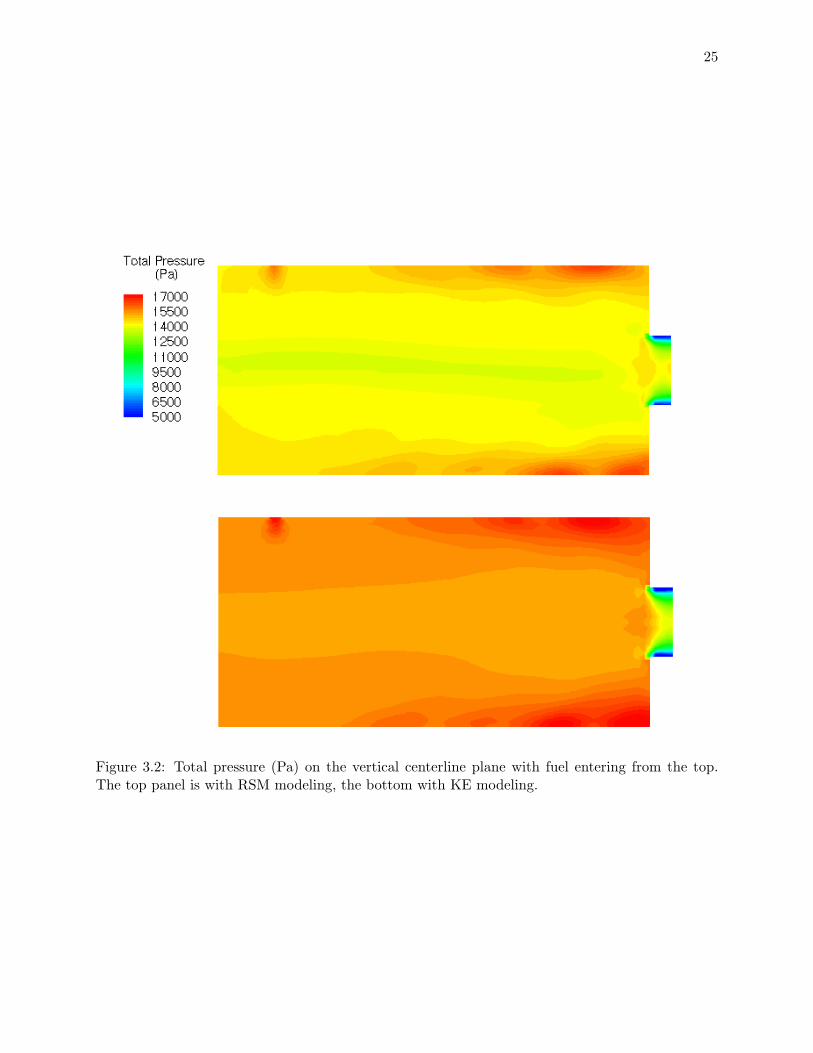
consistent with this. The total pressure on a longitudinal cut through the centerline is shown in

Fig. 3.2 for the RSM and k-ε model. While the overall drop in total pressure is comparable in the

two simulations, the contour plots show that the locations in the burner where total pressure is

lost are different. Since total pressure is lost due to viscous shearing, and viscous shearing causes

mixing of heat and species, differences in the total pressure field imply differences in mixing.

From the pressure and velocity data, it is apparent that the three turbulence models yield

generally similar predictions for the flow field, but that the predictions differ in some details. One

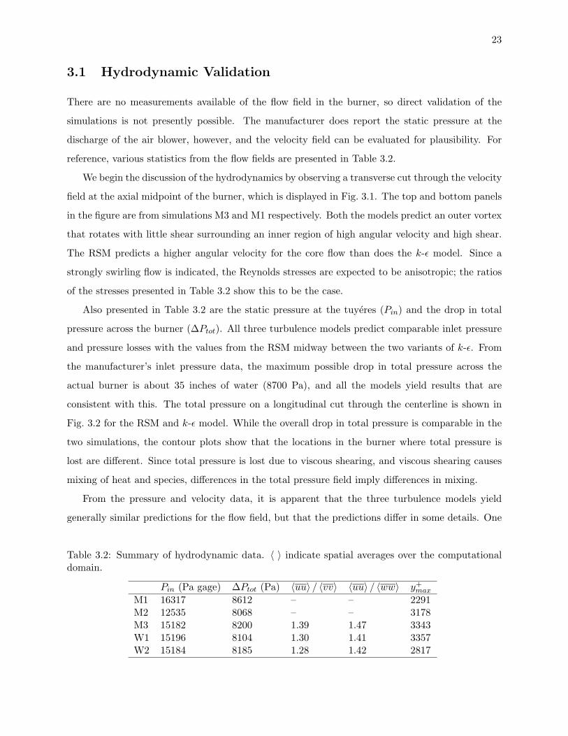
Table 3.2: Summary of hydrodynamic data. 〈 〉 indicate spatial averages over the computationaldomain.

Pin (Pa gage) ∆Ptot (Pa) 〈uu〉 / 〈vv〉 〈uu〉 / 〈ww〉 y+max

M1 16317 8612 – – 2291M2 12535 8068 – – 3178M3 15182 8200 1.39 1.47 3343W1 15196 8104 1.30 1.41 3357W2 15184 8185 1.28 1.42 2817

24

70.000065.000060.000055.000050.000045.000040.000035.000030.000025.000020.0000

VelocityMagnitude

(m/s)

Figure 3.1: Velocity magnitude (m/s) at the midplane. The top panel is with RSM modeling, thebottom with KE modeling.

25

Figure 3.2: Total pressure (Pa) on the vertical centerline plane with fuel entering from the top.The top panel is with RSM modeling, the bottom with KE modeling.

26

detail that is of particular interest in studies of non-premixed turbulent combustion is the local

strain rate, since shearing determines the rate of mixing, which affects the rate of chemical reaction.

From the plots of velocity and total pressure, it is apparent that k-ε, RNG (not shown), and RSM

yield different predictions for the size and location of the region of high shear inside the outer

vortex, and the question is which model most closely predicts the flow in the physical burner. An

examination of the derivations of the three turbulence models indicates that, if any of them can

yield good predictions, it is the RSM. As in most two equation turbulence models, an assumption

inherent in the k-ε and RNG models is that of Boussinesq (1877), i.e., that the Reynolds-stress

tensor can be related to the mean strain-rate tensor by an eddy viscosity. Wilcox (1993) notes

that among the applications for which this modeling assumption is not valid are flow over curved

surfaces, flow in rotating and stratified fluids, and three-dimensional flow; therefore, k-ε and RNG

are not expected to be effective for the current flow. Several researchers who have studied the

simulation of confined vortices and cyclonic combustors conclude that eddy-viscosity based models

are not appropriate for these flows (Boysan et al., 1986; Hogg and Leschziner, 1989a,b; Zhang

and Nieh, 1997). Based on the guidance from these sources, the RSM is used for the simulations

involving wood, which are the focus of this research.

3.2 Temperatures and Species Concentrations

In order to use the simulations to predict concentrations of pollutant species such as NOx, it is

first necessary to demonstrate that the predictions for the temperature and major species fields

are consistent with available data. Temperature and species data are shown in several formats in

Table 3.3 and Figs. 3.3 through 3.5.

We begin by considering exit plane temperatures and species concentrations since these values

can be compared with analytically determined limits. In Table 3.3 are shown the average tempera-

tures at the exit plane as predicted by FLUENT. Also shown are the adiabatic flame temperatures

assuming equilibrium composition and the fuel-air equivalence ratio (φ) used in the simulations.1

Since the equilibrium composition for the conditions simulated includes insignificant mole frac-

tions of combustion products other than H2O and CO2, the adiabatic flame temperature closely

approximates the upper limit of the exit plane temperature in the simulations.1The equilibrium values were computed using the UWeq code developed by D. T. Pratt considering fourteen

product species: H, HO2, H2, H2O, H2O2, O, OH, O2, CO, CO2, N2, N2O, NO, NO2.

27

In all simulations involving methane, the exit plane temperatures are less than the limiting

temperature, and the amounts by which they differ from the limit are consistent with the amount

of unburned fuel at the exit plane. The peak temperatures slightly exceed the limit predicted by

equilibrium analysis, which may be an artifact of the one-step reaction mechanism used in the

simulations; the equilibrium calculations take into account the effect the endothermic formation of

NO which occurs at high rates when the temperature is greater than 2200 K. In simulation M2, the

RNG turbulence model apparently retards mixing to an unrealistic extent; the amount of mixing

in M3 is less than that in M1, which is consistent with the excessive turbulent diffusion observed

when the k-ε model is used for swirling flows (Hogg and Leschziner, 1989a,b). The mass fractions

(Y ) of H2O and CO2 at the exit plane in the simulations involving methane are consistent with the

amount of unburned fuel and the exit plane temperatures.

In the simulations involving wood, the exit plane temperatures are slightly less than the predic-

tion by equilibrium methods, which is consistent with the levels of unburned CO, CH4, and C2H4

at the exit; the simulations predict complete burning of the char particles. The peak temperatures

observed in simulations W1 and W2 exceed the maximum possible based on equilibrium analysis,

but, as with methane, this is most likely an artifact of the reduced reaction set.

In Fig. 3.3 are shown the contours of static temperature on a longitudinal plane for simulations

M3 and W2. In both cases, a hot core is surrounded by cool air entering from the downstream

tuyeres. In the case of methane, the one-step reaction mechanism dictates heat release only where

fuel coexists with a considerable amount of oxidant, and there is a steep temperature gradient

where the burning occurs in a conical diffusion flame at the edge of the hot core. In simulation W2,

the temperature gradients are less steep and the diffusion flame is less pronounced. This is in part

Table 3.3: Summary of temperatures and species concentrations. The exit values are mass weightedaverages at the exit plane.

Peak Exit Exit Exit Exit Exit ExitT (K) T (K) YCO2 YH2O YCO YCH4 YC2H4

Equil. CH4 2225 1378 0.075 0.062 0 0 n/aM1 2277 1347 0.072 0.059 n/a 1.0× 10−3 n/aM2 2250 1199 0.062 0.051 n/a 9.1× 10−3 n/aM3 2244 1317 0.072 0.058 n/a 1.2× 10−3 n/aEquil. Wood 2136 1199 0.109 0.035 3.4× 10−9 n/a n/aW1 2012 1158 0.106 0.035 5.3× 10−3 1.2× 10−3 1.9× 10−3

W2 2004 1148 0.105 0.035 5.3× 10−3 1.2× 10−3 2.0× 10−3

28

due to the presence of significant amounts of CO which, in the context of the reaction

mechanism used in the simulations, requires less mixing of fuel and air before reaction

begins. The contours of O2 mass fraction (Fig. 3.4) show a core depleted of oxidant, a

diffusion zone, and an outer region rich in oxidant. As noted in the preceding paragraph, the

profiles for the wood and methane simulations are different, and some of this difference is

likely due to the grossly simplified reaction mechanisms assumed in the simulations. In the

methane simulation, and to a lesser extent in the wood simulation, little mixing occurs

between the core ow and the air entering through the downstream tuyeres. Further

investigation of this phenomena is warranted because if it exists in the physical burner

(rather than being an artifact of the simulations) it suggests an area in which burner

performance may be improved with respect to carbon conversion efficiency. The long, hot

central ame, however causes fuel-NOx to be reduced to N2 (see Chapter 4). The next contour

plots are of CO2 mass fraction (Fig. 3.5). Due to the selection of contour spacing, it is

especially apparent in this figure that unmixed air from the downstream tuyeres exits the

burner. Also evident in the lower panel of the figure are high concentrations of CO2 upstream

in the burner; these result from oxidation of the char particles directly to CO2. Since the W2

simulation shows oxidant levels to be extremely low in the upstream end of the burner where

the char oxidation is occurring, the effect of assuming that the char oxidizes to CO should be

evaluated. Finally, a contour plot of CO mass fraction for the W2 simulation is shown in Fig.

3.6. An exponential distribution of contour levels is used to emphasize the extent of the

incomplete combustion at the choke of the burner. When the plots of temperature, O2, and

CO are considered together, it is apparent that the simulation predicts a highly swirling

diffusion ame at the choke with cool air surrounding hot, partially burned gases. Density

stratification impedes the mixing of the fuel and oxidant. Mixing (and the resultant oxidation

of CO) downstream of the choke should cause the high levels of CO (of about 5000 ppm) to

significantly decrease.

29

Figure 3.3: Static temperature (K) on the vertical, centerline plane with fuel entering from the top.The top panel is from simulation M3 and the bottom is from simulation W2.

30

Figure 3.4: Mass fraction of O2 on the vertical, centerline plane with fuel entering from the top.The top panel is from simulation M3 and the bottom is from simulation W2.

31

Figure 3.5: Mass fraction of CO2 on the vertical, centerline plane. The top panel is from simulationM3 and the bottom is from simulation W2.

32

Figure 3.6: Mass fraction of CO on the vertical, centerline plane for simulation W2.

Chapter 4

NOx Production

In Chapter 3, it is shown that the temperatures and major species concentrations in simulation W2

are consistent with expected values and, therefore, that this simulation can be used as the basis for

predicting thermal and fuel NOx production in the McConnell burner. In the current chapter, the

W2 results were post-processed to predict NOx and HCN concentrations with various scenarios.

The overall results are shown in Table 4 below. The scenarios listed in the table span ranges of fuel

nitrogen content, volatile nitrogen content, and char BET surface area, with the first row in the

table representing reasonable estimates for wood dust and the last row representing estimates for a

wood dust containing a large amount of urea formaldehyde resin (Malte et al., 1996). The volatile

nitrogen is assumed to undergo devolatilization at the same rate as the carbon. The balance of the

nitrogen, i.e., the char nitrogen, undergoes conversion by heterogenous reaction. In the column of

Table 4 labeled “Max. Fuel NOx” are shown the fuel NOx concentrations that would occur if all the

fuel nitrogen were converted to NOx. In Figs. 4.1-4.5 are shown the NO and HCN concentrations

on the vertical cut through the centerline for each scenario; these figures are discussed below.

The fuel nitrogen concentrations are computed assuming that the char nitrogen is converted to

NO rather than to HCN, which is consistent with the earlier assumption that the carbon in the

char oxidizes to CO2 via (2.3a). When 93% of the fuel nitrogen devolatilizes, the conversion path

that the remaining 7% of the nitrogen takes has little impact on the total amount of NOx produced.

The value of 93% volatile nitrogen is selected to match the overall volatile yield of the wood dust

used in the modeling. However, to examine the impact of retention of nitrogen in the char, 50%

volatile nitrogen is also treated in the modeling.

The effect of thermal NOx on the total NOx emissions is shown in the table for each scenario.

33

34

Tab

le4.

1:N

Ox

mas

sfr

acti

ons

(Yi)

and

conc

entr

atio

nsat

the

exit

plan

eof

sim

ulat

ion

W2.

Mas

sfr

acti

ons

are×

106.

Con

cent

rati

ons

are

inpa

rts

per

mill

ion

dry

basi

sad

just

edto

18%

O2.

Scen

ario

Mas

s%

%of

NA

BE

TT

herm

alFu

elT

herm

al+

Fuel

NO

xM

ax.

Fuel

YH

CN

Nin

fuel

devo

l.(m

2/kg

)N

Ox

NO

xN

Ox

YN

Ox

ppm

vdY

NO

xpp

mvd

YN

Ox

ppm

vd#

/MM

Btu

app

mvd

W2-

10.

100.

9325

000

19.5

7.5

50.8

2069

26.5

0.18

510.

094

W2-

22.

830.

9325

000

19.5

7.5

373

145

0.97

1332

6.4

W2-

35.

650.

500

19.5

7.5

1088

421

2.82

2700

0.24

W2-

45.

650.

5025

000

19.5

7.5

845

327

857

332

2.22

2700

2.7

W2-

55.

650.

9325

000

19.5

7.5

570

221

581

226

1.51

2700

13

aN

Ox

ass

igned

the

mole

cula

rw

eight

of

NO

2

35

When only the model for thermal NOx is enabled, the NOx concentration at the exit plane is 7.5

parts per million on a dry volume basis adjusted to 18% O2 (ppmvd). Adjustment to 18% O2 is used

since this is the nominal O2 content found in the stack gas of dryers heated by dust-fired burners. In

the case of pure wood dust (0.1% nitrogen in the fuel), 7.5 ppmvd is a significant portion of the total

NOx emission. For the cases with higher fuel nitrogen contents, the thermal NOx is insignificant.

Also, the thermal and fuel NOx interact, so that the sum of the concentrations computed when each

mechanism is run separately are greater than the concentration predicted when the mechanisms

are run together.

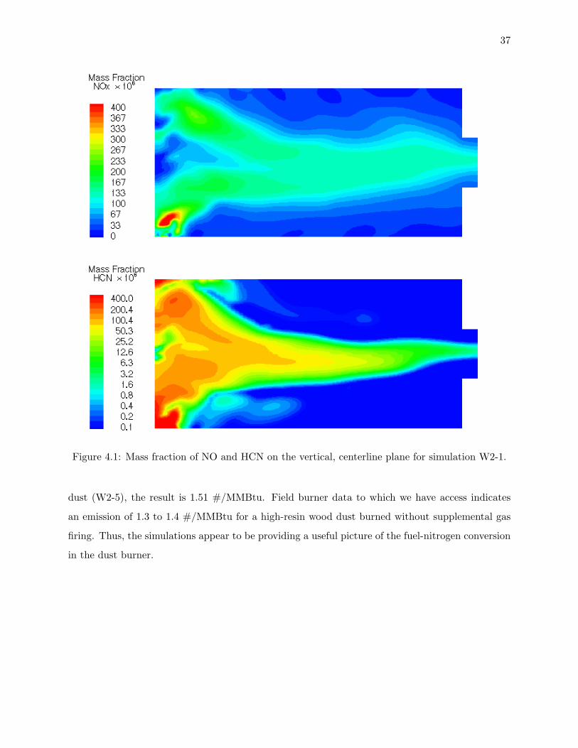
We begin our analysis of fuel NOx production with scenario W2-1 (Fig. 4.1). In this scenario,

93% of the fuel nitrogen is released from the wood particles in the volatiles so that the primary

path for production of NO is via HCN. The concentration of NO is shown in the top panel of the

figure and the concentration of HCN in the bottom panel. The HCN is produced very soon after

the volatiles are released from the particles as evidenced by the high concentration of HCN in the

inlet end of the burner away from the burner centerline. The HCN rapidly oxidizes to NO resulting

in the highest concentrations of NO in the upstream end of the burner. In the downstream section

of the burner, the competition between various fuel species for oxygen is strong in the diffusion

flame that is established with fuel species in the core of the burner surrounded by oxidant. At the

same time, the core region is hot enough (Fig. 3.3) to support the mutual destruction of HCN and

NO via the reduction reaction with the rate given by (2.29). Consequently, competition between

oxidation of HCN to NO and reduction of NO by HCN to N2 occurs, with the overall behavior

being a decrease in NO as the flow progresses downstream in the burner. The conversion of fuel

nitrogen to NO for this scenario is very high (52%).

The HCN is an intermediate of the fuel-nitrogen conversion process, and in the simulations, it

is the only fixed nitrogen species that links the fuel-nitrogen to the final products (NO and N2).

This simplification of the fuel-nitrogen conversion process results from basing the current model

mechanism on those presented in the literature on coal combustion. However, in wood flames, as

well as in flames for some ranks of coal, ammonia (NH3) also serves as a fixed-nitrogen intermediate.

Thus, in interpreting the present simulations, it may be best to regard HCN as a general fixed-

nitrogen intermediate. Although HCN surely exists in the flames of wood burners, its concentration

is probably less than indicated in the current simulations and NH3 is probably also present. The

lack of oxygen in the core of the combustor in the simulations also promotes the large concentrations

36

of HCN observed. The long, hot core and the surrounding diffusion flame are dominant features

of the present simulations and are consistent with a lack of O2 and an abundance of intermediate

fixed-nitrogen in the core.

In scenario W2-2 (Fig. 4.2), more nitrogen is added to the fuel to represent a dust of wood

containing resin; all other parameters are the same as in scenario W2-1. The formation and

destruction of NO is generally similar to that in the case of pure wood dust, but now, because

of the larger amount of fuel nitrogen, the HCN concentration in the core is very large, leading

to consumption of the O2 that penetrates there and reduction of NO to N2. The diffusion flame

surrounding the core flow is more pronounced. Consequently, the conversion of fuel nitrogen to

NOx in this scenario is only 11%.

In scenarios W2-3, W2-4, and W2-5 the fuel nitrogen is increased to the level observed in

the wood-with-resin dust analyzed by Malte et al. (1996). This is a “high-resin” fuel. In these

simulations, volatile nitrogen and the BET surface area (ABET) are varied in order to observe the

effect of the several situations for production and destruction of NO. In scenario W2-3 (Fig. 4.3),

the volatile nitrogen is reduced to 50%, and ABET = 0, which disables the reduction of NO on the

char surface. In the top panel of the figure, the concentration of NO in the core region is very high.

The surface reduction mechanism is unavailable to play an important role in the destruction of NO

in this region. Also, less HCN is available to reduce NO to N2.

In scenario W2-4 (Fig. 4.4), all parameters are the same as in W2-3 except the surface reduction

mechanism is enabled. The result is a substantial reduction in the NO concentration and an increase

in the HCN concentration at the exit plane. In scenario W2-5, it is assumed that the nitrogen in the

volatiles is proportional to the fraction of fuel mass that devolatilizes, i.e., 93%. This assumption

increases the amount of HCN that is formed and decreases the amount of NO formed directly.

However, due to the competition between the HCN oxidation and reduction reactions, a six-fold

decrease in the amount of NO formed directly results in a 32% decrease in NO at the exit plane.

The conversion rate for fuel nitrogen in scenario W2-5 is 8.4%, which is the lowest conversion of

fuel-nitrogen to NO observed in the simulations with high-resin fuel.

The preferred method of reporting NOx emissions for industrial burners is as pounds of NOx (as

NO2) per fuel input as millions of Btu on a HHV basis (MMBtu). The emissions are shown in these

units in Table 4. For the simulations of the wood dust without resin, the result is 0.18 #/MMBtu,

which is in the range expected for a wood dust burner. For the simulation of high-resin wood

37

Figure 4.1: Mass fraction of NO and HCN on the vertical, centerline plane for simulation W2-1.

dust (W2-5), the result is 1.51 #/MMBtu. Field burner data to which we have access indicates

an emission of 1.3 to 1.4 #/MMBtu for a high-resin wood dust burned without supplemental gas

firing. Thus, the simulations appear to be providing a useful picture of the fuel-nitrogen conversion

in the dust burner.

38

Figure 4.2: Mass fraction of NO and HCN on the vertical, centerline plane for simulation W2-2.

39

Figure 4.3: Mass fraction of NO and HCN on the vertical, centerline plane for simulation W2-3.

40

Figure 4.4: Mass fraction of NO and HCN on the vertical, centerline plane for simulation W2-4.

41

Figure 4.5: Mass fraction of NO and HCN on the vertical, centerline plane for simulation W2-5.

42

Chapter 5 Conclusions The focus of this research has been on the modeling and the prediction of NOx

concentrations in the cyclone wood dust burner. The FLUENT NOx model requires,

among other parameters, inputs for the fraction of fuel nitrogen that devolatalizes

and the BET surface area of the char, and neither of these quantities is well known

for wood dust. Decreasing the BET surface area has the same effect as decreasing

the volatile nitrogen fraction, i.e., it increases the exit plane NOx concentration.

Fortunately, the concentration of NOx at the exit plane increases by only a factor of

1.9 when the BET surface area is reduced from 25000 to 0 (m2=kg) and the volatile

nitrogen fraction is reduced from 93% to 50%. The conclusion is that modest

uncertainty in either of the input parameters will not lead to significant errors in

the NOx predictions. This encourages the thought that the development of the

current simulations can lead to insight into how to reduce NOx emissions from wood

dust burners.

Observation of the exit plane concentrations of CO and HCN indicate that the

chemical reactions are not complete by the time the gases pass through the choke of

the burner. Completion of reaction will occur downstream of the choke of the main

cyclonic combustion chamber modeled in this report.

43

Other Research on Modeling Wood Burners Other research conducted by the University of Washington Energy and Environmental Combustion Laboratory on the modeling of wood dust burners includes the following:

1. CFD modeling of a laboratory dust burner. This work will help to verify the modeling approach and the chemical rates, through the comparison of the modeling results to an existing data base for the laboratory burner.

2. CRN modeling of the laboratory and industrial wood dust burner. CRN stands for

Chemical Reactor Network. CRNs allow a much fuller chemistry to be applied to the problem, and generally permit faster computations. Thus, they can in general be used more easily by the design engineer than CFD.

These other researches are scheduled to be completed in 2005.

44

Other Research on Modeling Burners Other research conducted by the University of Washington Energy and Environmental Combustion Laboratory on the modeling of burners is focused on the following:

1 Development of global chemical kinetic mechanisms. 2 CFD and CRN modeling of lean premixed combustors, especially as used in low

emission power generation gas turbines

45

46

Acknowledgments

This research is supported by the U.S. Department of Energy (grant no. DE-FC07-001D13869).

Computing resources were provided by Intel Corporation and by the National Science Foundation

(grant no. DMI9617754). The authors thank Dr. Mark Ganter for assistance with the “Beowulf

cluster” used for the simulations.

Bibliography

Aho, M. J., J. P. Hamalainen, and J. L. Tummavuori (1993). Importance of solid-fuel properties

to nitrogen-oxide formation through HCN and NH3 in small-particle combustion. Combust.

Flame 95 (1-2), 22–30.

Anthony, D. B. and J. B. Howard (1975). Coal devolatilization and hydrogasification. AIChE J. 22,

625.

Badzioch, S. and P. G. W. Hawksley (1970). Kinetics of thermal decomposition of pulverized coal

particles. Ind. Eng. Chem. Process Des. Dev. 9, 521.

Baum, M. M. and P. J. Street (1971). Predicting the combustion behavior of coal particles. Combust.

Sci. Technol. 3 (5), 231–243.

Bilger, R. W. and R. E. Beck (1975). In 15th Symp. (Int’l.) on Combustion, pp. 541. The Com-

bustion Institute.

Blauwens, J., B. Smets, and J. Peeters (1977). Mechanism of “prompt” NO formation in hydro-

carbon flames. In 16th Symp. (Int’l.) on Combustion, pp. 1055–1064. The Combustion Institute.

Boussinesq, J. (1877). Theorie de l’ecoulement tourbillant. Mem. Presentes par Divers Savants

Acad. Sci. Inst. Fr. 23, 46–50.

Boyd, R. K. and J. H. Kent (1986). Three-dimensional furnace computer modeling. In 21st Symp.

(Int’l) on Combustion, pp. 265–274. The Combustion Institute.

Boysan, F., R. Weber, J. Swithenbank, and C. J. Lawn (1986). Modeling coal-fired cyclone com-

bustors. Combust. Flame 63 (1-2), 73–86.

Brunauer, S. (1943). The Absorption of Gases and Vapors. Princeton, NJ: Princeton University

Press.

47

48

Chen, J. C. and C. A. Lin (1999). Computations of strongly swirling flows with second-moment

closures. Int. J. Numer. Meth. Fl. 30 (5), 493–508.

de Soete, G. G. (1975). Overall Reaction Rates of NO and N2 Formation from Fuel Nitrogen. In

15th Symp. (Int’l.) on Combustion, pp. 1093. The Combustion Institute.

Field, M. A. (1969). Rate of combustion of size-graded fractions of char from a low rank coal

between 1200 K–2000 K. Combust. Flame 13, 237–252.

Flower, W. L., R. K. Hanson, and C. H. Kruger (1975). In 15th Symp. (Int’l.) on Combustion, pp.

823. The Combustion Institute.

Hanson, R. K. and S. Salimian (1984). Survey of Rate Constants in H/N/O Systems. In W. C.

Gardiner (Ed.), Combustion Chemistry, pp. 361.

Hogg, S. and M. A. Leschziner (1989a). 2nd-moment-closure calculation of strongly swirling con-

fined flow with large density gradients. Int. J. Heat Fluid Fl. 10 (1), 16–27.

Hogg, S. and M. A. Leschziner (1989b). Computation of highly swirling confined flow with a

Reynolds stress turbulence model. AIAA J. 27 (1), 57–63.

Kobayashi, H., J. B. Howard, and A. F. Sarofim (1976). Coal devolatilization at high temperatures.

In 16th Symp. (Int’l) on Combustion. The Combustion Institute.

Launder, B. E. and D. B. Spalding (1974). The numerical computation of turbulent flows. Computer

Methods in Applied Mechanics and Engineering 3, 269–289.

Leppalahti, J. and T. Koljonen (1995). Nitrogen evolution from coal, peat and wood during gasifi-

cation – literature-review. Fuel Processing Technology 43 (1), 1–45.

Levy, J. M., L. K. Chen, A. F. Sarofim, and J. M. Beer (1981). NO/Char Reactions at Pulverized

Coal Flame Conditions. In 18th Symp. (Int’l.) on Combustion. The Combustion Institute.

Lockwood, F. C. and C. A. Romo-Millanes (1992, September). Mathematical Modelling of Fuel -

NO Emissions From PF Burners. J. Int. Energy 65, 144–152.

Magnussen, B. F. and B. H. Hjertager (1976). On mathematical models of turbulent combustion

with special emphasis on soot formation and combustion. In 16th Symp. (Int’l.) on Combustion.

The Combustion Institute.

49

Malte, P. C. and D. G. Nicol (1997). Engineering analysis of NOx formation in wood dust burners:

Application to the Marshfield plant. Technical report, Department of Mechanical Engineering,

University of Washington.

Malte, P. C., D. G. Nicol, and T. Rutar (1996). Development of a model for predicting the NOx

emissions of burners fired with sawdusts and sanderdusts high in nitrogen. Technical report,

Department of Mechanical Engineering, University of Washington.

Monat, J. P., R. K. Hanson, and C. H. Kruger (1979). In 17th Symp. (Int’l.) on Combustion, pp.

543. The Combustion Institute.

Nunn, T. R., J. B. Howard, J. Longwell, and W. A. Peters (1985). Product compositions and

kinetics in the rapid pyrolysis of sweet gum hardwood. Ind. Eng. Chem. Process Des. Dev. 24 (3),

836–844.

Pope, S. (1985). Pdf methods for turbulent reactive flows. Progress in Energy and Combustion

Science 11, 119–192.

Smith, I. W. (1982). The combustion rates of coal chars: A review. In 19th Symp. (Int’l) on

Combustion, pp. 1045–1065. The Combustion Institute.

Smoot, L. D. and P. J. Smith (1985). Coal Combustion and Gasification. New York: Plenum Press.

Tillman, D. A. (1991). The Combustion of Solid Fuels And Wastes. San Diego: Academic Press.

Turns, S. R. (2000). An Introduction to Combustion. Concepts and Applications (2 ed.). McGraw-

Hill.

Westbrook, C. K. and F. L. Dryer (1984). Chemical kinetic modeling of hydrocarbon combustion.

Prog. in Energy and Combust. Sci. 10, 1–57.

Wilcox, D. C. (1993). Turbulence Modeling for CFD. La Canada, California: DCW Industries, Inc.

Williams, F. A. (1975). Turbulent Mixing in Nonreactive and Reactive Flows. New York: Plenum

Press.

Zhang, J. and S. Nieh (1997). Comprehensive modelling of pulverized coal combustion in a vortex

combustor. Fuel 76 (2), 123–131.