Simulation and modal analysis of instability and ...609183/FULLTEXT01.pdf · understanding. The...

Simulation and modal analysisof instability and transition in

a steady eccentric stenotic flow

Master ThesisJanuary 2013

Zeinab Moradi Nour

Department of MechanicsKTH Stockhom

Written with MiKTEX2.9, a pc implementation of LATEX

Abstract

Direct numerical simulation (DNS) of steady flow, with Re = 750 at inlet,through stenosed pipe has been done to study transition and turbulence of theflow in the post-stenosis area. The pipe has 75% constriction by area reduc-tion and 5% eccentricity of the main pipe diameter at the throat. A sinusoidalGaussian force is implemented to keep turbulent in the domain. The result showsacceptable agreement with previous study has been done by Fischer et al. [4]. Wesimulated the case by Nek5000 which benefits from the spectral element method(SEM) as a higher order accurate method. To have a better understanding of theturbulent flow, we have done the modal decomposition to obtain coherent struc-tures. Among several methods for modal decomposition, we considered ProperOrthogonal Decomposition (POD) and Dynamic Mode Decomposition (DMD)for current study. The methods have been implemented in Fortran, acceleratedusing OpenMP and is potentially settled for computation of large data sets.DMD implementation shows 2.5 speed up. The structures correspond to theimplemented force are extracted by POD however they have not been recognizedby dynamic decomposition.

3

Contents

Abstract 3

1 Introduction 13

1.1 Background . . . . . . . . . . . . . . . . . . . . . . . . . . . . . . 13

1.2 Present thesis . . . . . . . . . . . . . . . . . . . . . . . . . . . . . 14

2 Theory and formulation 15

2.1 Instability and Turbulence . . . . . . . . . . . . . . . . . . . . . . 15

2.1.1 Instability . . . . . . . . . . . . . . . . . . . . . . . . . . . 15

2.1.2 Turbulence . . . . . . . . . . . . . . . . . . . . . . . . . . 15

2.1.3 Statistical Analysis of Turbulent Flows . . . . . . . . . . . 16

2.1.4 Simulation of Turbulent Flows . . . . . . . . . . . . . . . 17

2.1.5 Discretization method . . . . . . . . . . . . . . . . . . . . 17

2.2 Modal decomposition . . . . . . . . . . . . . . . . . . . . . . . . . 18

2.2.1 Proper Orthogonal Decomposition (POD) . . . . . . . . . 18

2.2.2 Dynamic Mode Decomposition (DMD) . . . . . . . . . . . 21

3 Simulation 29

3.1 Simulation tool . . . . . . . . . . . . . . . . . . . . . . . . . . . . 29

3.1.1 Structure of each simulation . . . . . . . . . . . . . . . . . 29

3.2 Previous studies . . . . . . . . . . . . . . . . . . . . . . . . . . . 30

3.3 Formulation and simulation . . . . . . . . . . . . . . . . . . . . . 31

3.3.1 Physical interpretation of the flow . . . . . . . . . . . . . 35

4 Implementation 39

4.1 The main structure . . . . . . . . . . . . . . . . . . . . . . . . . . 39

4.1.1 POD subroutines . . . . . . . . . . . . . . . . . . . . . . . 40

4.1.2 DMD method . . . . . . . . . . . . . . . . . . . . . . . . . 43

4.1.3 Accelerating the code . . . . . . . . . . . . . . . . . . . . 44

5 Results 45

5.1 POD result . . . . . . . . . . . . . . . . . . . . . . . . . . . . . . 45

5.1.1 Validation . . . . . . . . . . . . . . . . . . . . . . . . . . . 45

5.1.2 POD result for stenosis pipe flow . . . . . . . . . . . . . . 47

5.2 DMD result . . . . . . . . . . . . . . . . . . . . . . . . . . . . . . 50

5.2.1 Validation . . . . . . . . . . . . . . . . . . . . . . . . . . . 50

5.2.2 DMD result for stenosis pipe flow . . . . . . . . . . . . . . 50

6 Conclusion 57

6 CONTENTS

Acknowledgements 59

List of Figures

1.1 The local restriction of the artery. Borrowed from U.S. NationalLibrary of Medicine website. . . . . . . . . . . . . . . . . . . . . . 13

3.1 Working flow overview. . . . . . . . . . . . . . . . . . . . . . . . . 30

3.2 Side and front views of the stenosis geometry (L = 2D). Thedashed line shows the 0.05 offset from the main axis of the pipe(borrowed from [4]). . . . . . . . . . . . . . . . . . . . . . . . . . 32

3.3 The turbulent kinetic energy, a)xz-plane b)yz-plane, comparisonfor two sets of snapshots for N = 12 and N = 16 shows a coinci-dent, therefore N = 12 is suitable resolution. . . . . . . . . . . . 33

3.4 Layout of spectral element mesh with k = 11153 hexahedral cells. 33

3.5 The center-line velocity contour for the case before applying theforce. . . . . . . . . . . . . . . . . . . . . . . . . . . . . . . . . . 34

3.6 The position of the force in the pipe. . . . . . . . . . . . . . . . 34

3.7 The center-line velocity contour for the case after applying theforce starting from time unit 222. . . . . . . . . . . . . . . . . . 35

3.8 The rms-velocity shows acceptable agreement with the last threetime intervals for xz-plane (y= 0) and yz-plane (x= 0). Each sym-bol represents the start point of these three intervals. It is assumedthat the turbulent flow is reached to the statistically steady state.Furthermore, w rms velocity profile in xz-plane shows existence ofthe hairpin vortices in the interval 0 < z/D < 4. . . . . . . . . . 36

3.9 The turbulent kinetic energy shows acceptable agreement with thelast three time intervals for xz-plane (y= 0) and yz-plane (x= 0).Each symbol represents the start point of these three intervals. Itis assumed that the turbulent flow is reached to the statisticallysteady state. . . . . . . . . . . . . . . . . . . . . . . . . . . . . . 36

3.10 Stream-wise instantaneous velocity magnitude plot at 247, yz-plane cut. . . . . . . . . . . . . . . . . . . . . . . . . . . . . . . . 37

3.11 The negative velocity in post stenosis area. . . . . . . . . . . . . 37

3.12 Stream-wise velocity cross sections: 2D (top left), 4D (top right),6D (down left) and 8D (down right). . . . . . . . . . . . . . . . . 37

3.13 Negative contour -2.0 λ−2 values represent instantaneous coherentstructures in the turbulent region between 4D < z < 14D . . . . 38

3.14 The mean velocity profile defined by ensemble average. . . . . . 38

4.1 Matrix multiplication of xTx where ch(i, j) denotes each chunkand chxTx(i, j) denotes one block in solution. . . . . . . . . . . . 41

4.2 The number of chunks effects on cputime of running pod snap for60 snapshots. . . . . . . . . . . . . . . . . . . . . . . . . . . . . . 42

7

8 LIST OF FIGURES

4.3 The optimum number of threads for pod snap is 8. . . . . . . . . 44

5.1 Spatial modes 1, 3 and 5 (a) computed by pod orig and (b) com-puted by pod snap are match together. . . . . . . . . . . . . . . 45

5.2 Logarithmic plot of energy spectrum correspond to most energeticPOD modes. . . . . . . . . . . . . . . . . . . . . . . . . . . . . . 46

5.3 First 5 temporal modes (a) computed by pod orig and (b) com-puted by pod snap shows a complete agreement. Mode zero is al-most constant and two pairs of next modes were plotted together,showing phase shift in time. . . . . . . . . . . . . . . . . . . . . . 46

5.4 Orbit plot of temporal modes 1 and 2 showing periodic motion oftravelling structure correspond to these modes. . . . . . . . . . . 46

5.5 Reconstructed travelling structures by 1 and 2 spatial modes (a)computed by pod orig reconstruct and (b) computed by pod snap reconstruct

shows perfectly match together. . . . . . . . . . . . . . . . . . . . 47

5.6 (a) Initial snapshot from flow field (b) snapshot from reconstructedflow with pod snap reconstruct by all computed modes by pod snap

to validate the result. . . . . . . . . . . . . . . . . . . . . . . . . 47

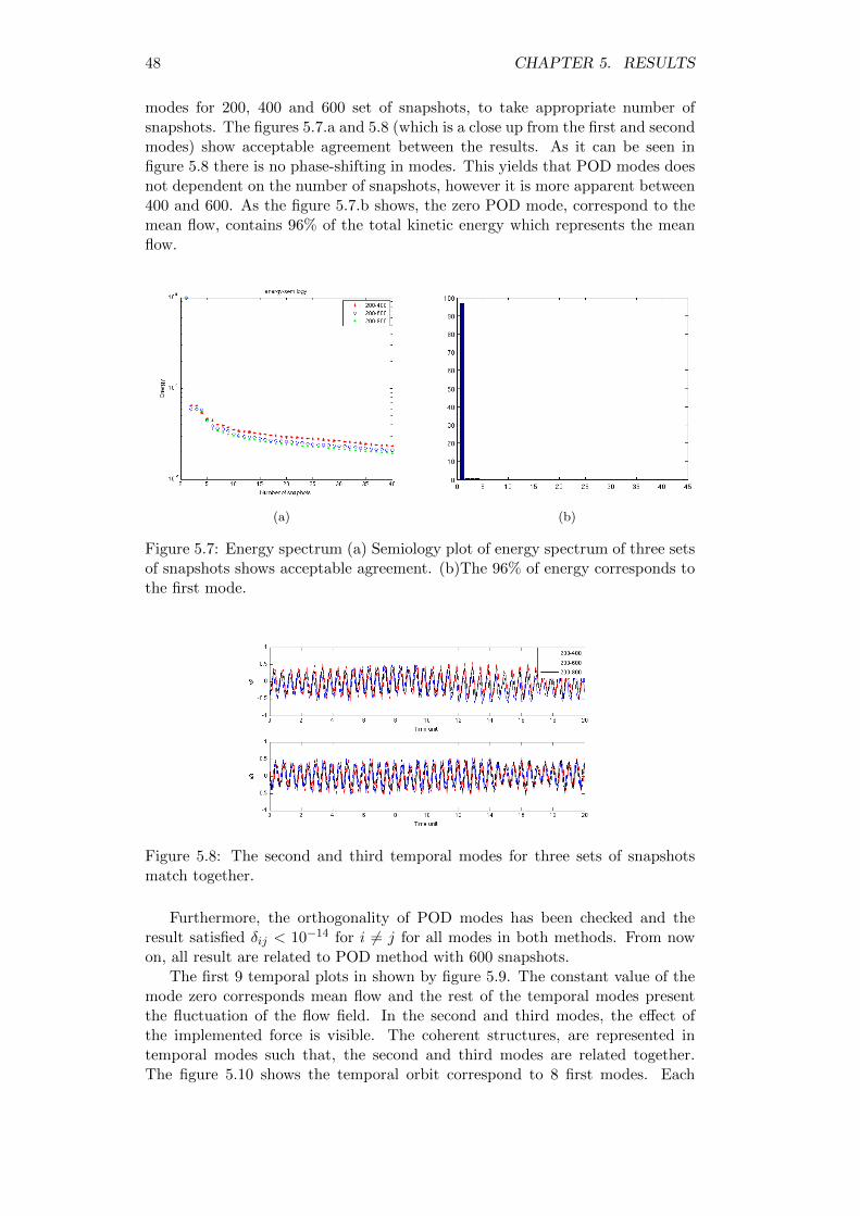
5.7 Energy spectrum (a) Semiology plot of energy spectrum of threesets of snapshots shows acceptable agreement. (b)The 96% ofenergy corresponds to the first mode. . . . . . . . . . . . . . . . . 48

5.8 The second and third temporal modes for three sets of snapshotsmatch together. . . . . . . . . . . . . . . . . . . . . . . . . . . . . 48

5.9 Temporal ,plot:(a) Mode zero corresponds mean flow, has constantvalue. (b) The first and second modes shows the effect of the force. 49

5.10 Temporal orbit in subspace spanned by (a)v1 and v2 (b)v3 and v4(c)v5 and v6 (d) v7 and v8 vs time. . . . . . . . . . . . . . . . . . 50

5.11 Velocity iso-contours of reconstructed travelling structure by (a)spatial modes 1 and 2 for (−0.3, 0.3).(b) by spatial modes 5 and6 for (−0.1, 0.1). (c) spatial modes 7 and 8 for (−0.1, 0.1) and (d)low frequnecy spatial modes 4-9 for (−0.1, 0.1) found according tothe figure 5.12 . . . . . . . . . . . . . . . . . . . . . . . . . . . . . 51

5.12 Distribution of energy among modes . . . . . . . . . . . . . . . . 51

5.13 Energy spectrum and Ritz values of 2D flow passing a cylinder (a)The energy computed by |D−1|2, shows only one energetic modewith low frequency. (b) Ritz values on unit circle . . . . . . . . . 52

5.14 Comparison of first computed dynamic mode with (a) existingMATLAB code and (b)mode.f90 for 2D flow passing a cylinder. 52

5.15 (a) Initial snapshot from flow fields (b) Reconstructed snapshotby all computed mode for 2D flow passing a cylinder . . . . . . 53

5.16 Ritz values located on unit circle, stenosis pipe flow in 3D. . . . . 54

5.17 The energy of computed modes (a) consist of energy correspond tothe mean flow and force. (b) The energy correspond to the meanflow and implemented force has been removed for 3D stenosis pipeflow. . . . . . . . . . . . . . . . . . . . . . . . . . . . . . . . . . . 54

5.18 Velocity iso-surface (−4, 4) plot of the first dynamic mode cor-responds to the implemented force. The structures captured byPOD for the same mode can not be recognized here. . . . . . . . 55

LIST OF FIGURES 9

5.19 Stream wise velocity magnitude plot corresponds to the time 247.The reconstructed flow field presented in figure (b) is the same asthe initial snapshot generated by Nek5000 in figure (a). . . . . . 56

10 LIST OF FIGURES

List of Tables

4.1 Memory requirement and sequential time of running POD orig onEllen for three sets of snapshots. . . . . . . . . . . . . . . . . . . 42

4.2 Comparison between running the code for two methods pod origand pod snap (50 chunks) for 200 snapshots. . . . . . . . . . . . 43

11

12 LIST OF TABLES

Chapter 1

Introduction

1.1 Background

Stenosis pipe flow, as a model for arterial stenosis, was the subject for manyexperimental ([3]) and computational studies with different hypothesis. The localrestriction of the artery (heart vessels) which is a result of the accumulation offatty-plaque in the walls of the large arteries, is called Atherosclerosis whichcan be a reason for Artery Disease, thrombosis, heart attack and stroke. Flowseparation in combination with loosing pressure, can reduce the flow rate andcause localized absence of oxygen which is an indicator for surgical interferences.Stenoses are commonly characterized as a percentage reduction in diameter orarea of the host vessel and are clinically considered significant when the areareduction is greater than 75%. In most cases, eccentricity is a characteristic ofthe arterial stenosis.

Figure 1.1: The local restriction of the artery. Borrowed from U.S. NationalLibrary of Medicine website.

The pulsatile (caused by cyclic pumping motion of the heart), low Reynoldsnumber (relevant to human physiology) flow in combination with strong shearlayer can cause transition of flow to turbulence in post-stenotic area which leadsto heart attack or if it happens in one of the major vessels supplying the braincan lead to a cerebral stroke [2]. Therefore, studying stenosis artery has animportant role to prevent progression of diseases and cure.

13

14 CHAPTER 1. INTRODUCTION

1.2 Present thesis

A complex turbulent flow is superposition of spatially coherent, temporally evolv-ing vortical motions which is called coherent structures[19]. The study of domi-nant and coherent structures in turbulent flows was always challenging due to un-steadiness, three dimensionality and stochastic characteristics of turbulent flows.These coherent structures are responsible for the bulk mass, momentum and en-ergy transfer [11]. Analysing these structures by decomposing the flow into themodes is a common approach. Among several decomposition methods, ProperOrthogonal Decomposition (POD) and Dynamic Mode Decomposition (DMD)which have been applied to study the physics of the dynamics of the flows arewidely used in different applications. Developing a package to implement thementioned methods on the cases that contain turbulent flow, was the aim of thecurrent study. As a test case for the code a pipe with rigid wall and constrictionin upstream has been chosen. The Direct Numerical Simulation of the flows in a75% stenotic pipe flow (by area reduction) with 5% eccentricity position of theconstriction has been studied previously by [4]. These conditions cause transitiona laminar jet-like to a (quasi-)turbulent state in post-stenosis area depending onthe Reynolds number which in most cases are dominated by a clear sheddingfrequency. The proper prediction of this changeover is crucial for an improvedunderstanding. The physical goal of the study is the numerical investigation ofthe turbulence breakdown downstream of the stenosis area.

In order to simulate and discretize the flow numerically, the Nek5000 isused to apply Direct Numerical Simulation (DNS) and Spectral Element Method(SEM). Nek5000 is a parallel, modular, open source code, written in Fortran 77,and is able to scale up to 250000 processors. In Nek5000, there is an interface tovisIt for visualization and post-processing, which is used also during the presentstudy [18].

To have a better understanding of the POD and DMD theory, a comparisonbetween some more common algorithms, introduced in previous papers, has beendone and is presented in §2. The explanation about simulation process and toolsis given in §3. In §4, there is description about the code development. Theresults and conclusions will be discusses in §5 and §6 respectively.

Chapter 2

Theory and formulation

Study transition of jet flow to turbulence in stenosis pipe flow needs initial knowl-edge about instability and turbulence. Therefore in the following sections somedefinition related to the subject will be mentioned. Furthermore, there will be adiscussion about theory of different methods of POD and DMD.

2.1 Instability and Turbulence

2.1.1 Instability

The hydroynamic stability theory deals with this problem that how the laminarflow responses to forces or disturbances with small or moderate amplitudes. Inthis context, a flow is called stable if it turns back to the original laminar state,otherwise it goes to unstable state and often there is a changeover to turbulence[15]. According to the definition of the stability, if there is a decreasing inenergy of the perturbation as the time proceeds, the flow is going to be stable,otherwise depending on the initial perturbation, it can be stable or unstable.There are three types of evolution of disturbances; evolution of disturbancesthat are localized in space, evolution of an unstable wavelike disturbance intime, and the oscillatory disturbances localized in space. In a case that thesource of disturbance is fixed (first type of evolution), then the temporal growthis not an appropriate characteristic to define stability with. In absence of boundfor disturbance growth, as the stream-wise distance goes to infinity, the flowbecomes unstable. For stenosis pipe flow as we waited till the turbulent flowreaches near fully developed situation (statistically steady state), therefore wecan assume that there is no temporal growth in time and instead there could bea growth in space.

2.1.2 Turbulence

For all flows, there is a critical Reynolds number where below this critical point,the flow is laminar and above this point there is a transition to truculence.Receiving energy from an external energy source (e.g. the mean flow) causes theturbulent flow to be sustained. Interaction between large scale and small scale isknown as the cascade process. In the cascade process, the energy transfers fromthe larger scales (eddies) to the smaller scales. This means that the viscositytakes progressively important role up to final stage that kinetic energy dissipatesto heat (by viscous dissipation, ε). The largest structure in a turbulence flow

15

16 CHAPTER 2. THEORY AND FORMULATION

is limited by the geometry i.e. the large vortical structure in a pipe is equalto its diameter while smallest scale has no dependency to the geometry. Theviscosity and viscous dissipation are the only important factors in smallest scalesor Kolmogorov scales. The quasi-equilibrium is a situation when transformingenergy into heat in small scales is in balance with the energy that transfers fromlarge scale to small scale. There are some characteristics of the turbulent flowsthat other approaches, that can be used for other problems in fluid mechanics,become useless [17]. These characteristics can be listed as below:

• Stochastic behaviour: there is still no applicable simplification in statisticalmechanics.

• Strong dependency in space and time: It is not easy to be modelled.

• Non-linearity: linearisation destroys the problem.

• Presence of vorticity (rationality).

• Three dimensionality.

All turbulent flows are described by statistical fluctuations of all variables (e.g.velocity, pressure, density, temperature, etc.) around mean flow. For instancethe perturbed values for velocity and pressure can be defined as Ui + u′i andP + p′ where the (Ui, P ) denote the basic state [15]. Therefore by applying theperturbed variables (U) on Navier-Stokes equation and subtracting it from thebasic state, we get the disturbance non-linear equations for incompressible flowsas,

∂u′i∂t

= − ∂p

∂xi− Uj

∂u′i∂xj− u′j

∂Ui∂xj

+1

Re∇2u′i − u′j

∂u′i∂xj

,

∇u = 0

(2.1.1)

which is the equation for evolving system with initial disturbance u0i = ui(t = 0)and will be complete by appropriate boundary conditions.

2.1.3 Statistical Analysis of Turbulent Flows

As it is mentioned in the last section, the Navier-Stokes equation can be usedto study turbulent flows. However, since ui(u, v, w) is a random variable (itis the summation of the mean flow and fluctuations), to study turbulent flowone needs to define the concepts which cover its properties. To have a betterunderstanding of a turbulent flow, we need to analyse development of somestatistical quantities. First, we introduce two types of averages; averaging overtime and ensemble average. These averages are equivalent for steady mean flow.The averaged velocity is commonly shown by ui(x, t) where x = (x, y, z). Thegeneral definition of the average over time is,

ui(x) = limT→∞

1

T

∫ T

0ui(x, T0 + t)dt (2.1.2)

and the ensemble average over number of observation or snapshots of the flowwhich are obtained from experiments or numerical simulations is,

2.1. INSTABILITY AND TURBULENCE 17

ui(x) = limn→∞

1

n

n∑j=1

ui(x, tj). (2.1.3)

The velocity deviation from mean value is called fluctuation,

u′i = ui − ui. (2.1.4)

Also, the rms-value of u can be defined by,

urms = u′u′1/2

(2.1.5)

As u′u′, v′v′ and w′w′ introduce the kinetic energy per unit mass of the velocityfluctuations in each direction, therefore the Turbulent Kinetic Energy is definedas,

K =1

2u′iu′i (2.1.6)

that is presented in Einstein summation convention notation (u′iu′i+v

′iv′i+w

′iw′i).

If u′i = 0, 2.1.6 becomes,

K =1

2(u2i − u

2i ) (2.1.7)

2.1.4 Simulation of Turbulent Flows

Direct Numerical Simulation (DNS) and Large Eddy Simulation (LES, used ata lower level of approximation) are two methods that can be used to model tur-bulent flows. The most important currents in analytical studies of turbulenceare statistical and deterministic. However, there are some disadvantages withthese approaches such as closure problem and limited criterion in studying andanalysing only transition and pre-turbulence. Solving the Navier-Stoke equationnumerically, without turbulence modelling is an important advantage of DNS[6]. As well as having a higher order of accuracy, it gives possibility to do thecomputation on complex geometries with non-conformal meshes in local refine-ments. However, increasing the Reynolds number make this method challengingand expensive (according to the reciprocal proportion of the smallest turbulent

eddies to Re34 ) specially in the flows with inhomogeneous turbulence. Therefore

it is limited to the cases with simple geometries and low Reynolds number.

2.1.5 Discretization method

Spectral Element Method (SEM), a higher-order accuracy method, is a commonmethod to apply to the DNS of the fluid flow with moderate Reynolds number.This method provides both efficiency of global spectral method and geometryflexibility of the finite elements method, provided by non-conforming deformedhexahedral elements [4]. Initial step to solve the Navier-Stokes equation is todecouple the equation into two elliptic sub-problems [16]. The spectral elementspatial discretization is based on representing the weak form of the Helmholtz


equations on domain Ω. In the next step the domain is subdivided to K macro-(spectral)elements and is expanded the solution, data and test function withineach sub-domain, in terms of Nth-order tensor product polynomials. The al-gorithm proceeds as the Legendre spectral element method uses the mappedLagrangian interpolant bases on −1 to 1 interval (depend on dimension). TheGauss-Lobatto quadrature assure the accurate approximation to apply the ob-tained ansatz for u (velocity variable) into weak integral. The result of thisdiscretization is a linear system of equation that the rest of the process concernsto solve this system.

2.2 Modal decomposition

As the simulation of the flow does not give understanding about the underly-ing dynamics in it, there is a need to perform an analysis on the result of thesimulation. On the other hand coherent structures approach to turbulence givesdifferent picture, based on this idea that some turbulent are not so complicatedthat they look like at first sight. In another word, such flows are assumed to becomposed of the set of organized motions with simple spatial structures. Com-plexity of these kind of turbulent flows generated by the superposition in spaceand time of these organized, so-called coherent structures[21]. Applying modaldecomposition to identify coherent structures and dynamics of the evolving flowfield is a solution to overcome the difficulties of the study of turbulent flows.The set of the modes obtained by modal decomposition can be represented asthe reduced-order basis that is a approximation of the original flow. There aredifferent decomposition techniques derived previously, but in the current studytwo of them will be considered; Proper Orthogonal Decomposition (POD) andDynamic mode decomposition (DMD).

2.2.1 Proper Orthogonal Decomposition (POD)

The Proper Orthogonal Decomposition (POD) is originally proposed by Lumleyin 1967. POD is a method to extract a basis for a modal decomposition froma set of snapshots and rank them by their energy. The energetic structures canbe captured in transitional, weak turbulent flows and in a case that large scaledynamic (hairpin vortices) exist in turbulent flows [8]. It is possible to show thatthe POD decomposition is optimal for modelling and reconstructing a signalu(x, t) (see more in [7]). The following explanation is according to the procedurethat presented by Manhart et al. [7] about the theory of the POD. Assumeu(x, t) is a turbulent flow field and the velocity vector u = (u, v, w), is definedin physical space x = (x, y, z) and time t. The data for velocity can be obtainedeither by measurement as a result of the experiment or by numerical simulationin discrete points and stored in matrix U . The time-space dependent velocityfield can be expanded into orthogonal basis functions φ

n(x) = (φn1 , φ

n2 , φ

n3 )(x) in

space, and orthogonal time coefficients an(t) (see more about orthogonality in[7]). Therefore, if NM is number of the modes that we want to extract, we have,

ui = (x, t)→ U =

u(x1, t1) . . . u(xNp , t1)...

. . ....

u(x1, tNT ) . . . u(xNp , tNT )

(2.2.1)

2.2. MODAL DECOMPOSITION 19

an(t)→ A =

a1(t1) . . . aNM (t1)

.... . .

...a1(tNT ) . . . aNM (tNT )

(2.2.2)

φni (x)→ Φ =

φ1(x1) . . . φ

1(xNp)

.... . .

...

φNM (x1) . . . φ

NM (xNp)

(2.2.3)

in which, Np = Nx.Ny.Nz is the number of grid points, NT is the number ofsamples or snapshots that are taken in time and NM is the number of modes.The idea behind POD is to find a basis function φi(x) and coefficient a to de-compose the velocity field u such that,

ui(x, t) ≈NM∑n=1

an(t)φni (x) (2.2.4)

Therefore, one can say that the goal of POD is to find the proper orthogonalbasis Φ by solving the minimization problem,

min R for a and φ, where R =

∫T

∫ ∫ ∫v(ui(x, t)−

NM∑n=1

an(t)φni (x))2dxdt

(2.2.5)

Solving the mentioned minimization problem leads us to two equivalent eigen-value problems for A and Φ. The first one is original eigenvalue problem of thespatial modes, proposed by Lumley (1967)[7],

1

NTUTUGΦT = ΦTΛ,

∫∫∫vRij(x, x

′)dx′ = λnφni (x). (2.2.6)

in which, G is a diagonal matrix and contains the coefficients of the discretequadrature use to approximate the integral. The second one eigenvalue problemfor temporal modes that is used for the number of snapshots are sampled in time,

1

NTUGUTA = AΛ,

∫TC(t, t′)an(t′)dt′ = λnan(t) (2.2.7)

These eigenvalue problems were called “direct method” and “methods of snap-shots” by Sirovich in 1987 [7]. The spatial correlation tensor Rij(xx

′) and itstemporal counterpart C(t, t′) in these equations can be defined as,

R =1

NTUTUG, Rij(x, x

′) =1

T

∫Tui(x, t)uj(x

′, t)dt (2.2.8)

C =1

NTUGUT , C(t, t′) =

1

T

∫∫∫vui(x, t)ui(x, t

′)dx (2.2.9)

Because of the weighting function G, the matrix UTUG is not symmetrical. Butfor numerical purpose, it is possible to make it symmetrical by using a similaritytransformation with G1/2 [7]. As it is mentioned before, each eigenvalue represent


the energy content correspond to its mode and the total energy can be obtainedby summation of these eigenvalues.

Instead of solving eigenvalue problem, one can use SVD for POD. Therefore,applying SVD on matrix U we have,

U = ΦΣV T (2.2.10)

where, Φ is matrix of spatial modes, V is matrix of temporal modes and Σcontains sorted singular values on its diagonal.

As we discussed above, the method of the snapshots is another method toimplement POD on a data field, which solves eigenvalue problem or SVD onUTU (specially in case of rank deficiency). This could be a faster method if thesize of UTU is much smaller than U . Therefore we have,

UTU = (ΦΣV T )T (ΦΣV T ) = V Σ2V T . (2.2.11)

The non-zero singular values of matrix U are the square roots of the non-zeroeigenvalues of UUT and UTU and can be used to obtain the energy. Therefore,the energy is the square root of diagonal elements of Σ. As we have the rightsingular vectors matrix then the left singular vectors of matrix U , and pod modescan be calculated as,

Φ = UV Σ−1 (2.2.12)

Computing energy either by solving an eigenvalue problem or by applying SVDone can recognize the most energetic structures of the system. It is possibleto reconstruct the flow by these energetic structures according to the equation2.2.4.

Reconstructing travelling structures

As POD separates the flow in space and time, therefore one can reconstruct thetravelling structures according to the coherence structures in the flow filed. Tofind these coherence structures, understanding characteristic of the flow is theinitial step.

Assume the flow contains a pure travelling mode, therefore the equation ofthe wave can be defined as,

f(x, t) = ei(αx−ωt) = sin(αx− ωt). (2.2.13)

By implementing relation of difference of trigonometric functions and rewrite thewave equation we have,

f(x, t) = sin(αx− ωt) = sin(αx). cos(ωt)− cos(αx). sin(ωt) (2.2.14)

where, α and ω are real. The right hand side of this equation shows that thistravelling structure contains two modes. The sin(αx) and cos(αx) denote the


Topo-modes (spatial modes) and the cos(ωt) and sin(ωt) denote the Chrono-modes (temporal modes). Therefore, reconstructing a pure travelling requirestwo modes. For the case that the flow has growth in space, α has both real andimaginary parts. In that case the equation 2.2.13 can be separated into real andimaginary parts,

f(x, t) = eαix.ei(αrx−ωrt) (2.2.15)

The only difference between last equation and 2.2.13 is an extra coefficient.Therefore, it shows that to reconstruct coherent structures only two modes aresufficient.

In real flow, it is not easy to recognize structures that a wave is composedby, therefore one solution is to look at the phase portrait of each two similarmodes. This is possible by analysing parametric plot as a function of time. Theparametric plot represents the periodic behaviour of related modes.

2.2.2 Dynamic Mode Decomposition (DMD)

However, POD is a method that can be applied for experimental or numeri-cal snapshots to obtain the energetic structures, but there are some drawbackswhich may not give the correct understanding of the dynamics in the flow. Forinstance, ranking only by energy may not cover all circumstances that the flowstructures can be ranked by [9]. Therefore those modes captured by POD containlarge range of frequencies. There is another decomposition method according tothe Koopman analysis which can be applied on dynamic systems and is calledDynamic Decomposition. The method finds the eigenvalues and eigenvectors ofnon-linear dynamics of the flow that are approximated according to the eigen-values and eigenvectors of the linear model [13]. The frequencies and growthrate of each mode can be obtained by magnitude and phase of its correspond-ing eigenvalue. In the following, there is a brief explanation about the theory ofKoopman operator and DMD and also a comparison between different approachsto implement them.

• Koopman Operator

Rowley et al. [13] define Koopman operator as below,

Definition: Consider a dynamical system evolving on a manifold M suchthat, for all xi ∈M

xi+1 = f(xi) (2.2.16)

where f is a map from M to itself and i is an integer index. The Koopmanoperator is a linear operator U that acts on scalar-valued functions on M inthe following manner: for any scalar-valued function g : M → R, U mapsg into a new function Ug given by

Ug(x) = g(f(x)). (2.2.17)

Then, there is a unique expansion [10] that expands each snapshot in terms


of φj or Koopman eigenfunctions and vector coefficients vj which are calledKoopman modes, so

g(x) =

∞∑j=1

φj(x)vj (2.2.18)

Now, iterates of x0 are given by

g(xk) =

∞∑j=1

λkjφj(x0)vj , (2.2.19)

In this equation λj∞j=1 or Koopman eigenvalues dictates the growth rateand frequency of each modes.

• General description for DMD

The general idea of modal decomposition for non-linear systems can bedefined as below.

Suppose that XN1 is a collection of snapshots:

XN1 = x0, x1, . . . , xN (2.2.20)

which is collected in a constant sampling time ∆t. Let, λj and vj be theempirical Ritz values and vectors of this sequence. Assume λj ’s are distinct.Then

xk =

N∑j=1

λkj vj , k = 0, . . . , N − 1 (2.2.21)

where vj denotes modes and λj has the same definition that is mentioned

for Koopman expansion. One can write vj = v(0)j dj , where norm of vj is 1

and dj is called amplitudes of the modes [14]. Let, V (0) denotes normalizedmodes matrix and V (1) includes vj . Therefore the matrix form of 2.2.21 is,

XN−10 = V (1)N1 S or XN−1

0 = V (0)N1 D(1)S (2.2.22)

where D(1) is a diagonal matrix containing amplitudes and is called scalingmatrix V (1) = V (0)D(1). Also the matrix S is the so-called Vandermondematrix,

S =

1 λ1 λ21 . . . λN−11

1 λ2 λ22 . . . λN−11...

......

. . ....

1 λN λ2N . . . λN−1N

. (2.2.23)

According to this expansion one can say that DMD algorithm approximatesKoopman modes and eigenvalues from a finite set of data [10]. The idea


behind this decomposition is close to the Arnoldi method. Therefore, weare going to explain how the space that is constructed by linear mappinggives information about Ritz values and dynamic modes.

Assume x0, x1, . . . , xn is a data sequence generated by a nonlinear systemand also f(x) = Ax where A is a linear mapping that maps each snapshotto the next one, such that

xi+1 = Axi (2.2.24)

this gives another representation of snapshots data set as below

XN−10 = x0, Ax0, A2x0, . . . , A

N−1x0. (2.2.25)

We perform an analysis on the flow by extracting dynamic characteristics(eigenvalues, eigenvectors, energy amplification, etc.). Suppose that we canwrite last snapshot xN as a linear combination of previous N − 1 vectors,for a sufficiently long sequence of the snapshots. Thus

xN = c0x0 + c1x1 + · · ·+ cN−1xN−1 + r (2.2.26)

or in the matrix form

xN = XN−10 c+ r (2.2.27)

in which cT = c0, c1, . . . , cN−1 and r is the residual vector. Also we havethe following relations,

Ax0, x1, . . . , xN−1 = x1, x2, . . . , xN = x1, x2, . . . , XN−10 c+ reTN−1

(2.2.28)

or in the matrix form,

AXN−10 = XN

1 = XN−10 C + reTN−1 (2.2.29)

in which C is known as the Companion matrix,

C =

0 0 . . . 0 c01 0 . . . 0 c1...

. . ....

...0 . . . 1 0 cN−20 . . . 0 1 cN−1

. (2.2.30)

The straight consequence of 2.2.29 is that decreasing the residual increasesthe overall convergence and therefore the eigenvalues of C will converge


toward some eigenvalues of A. In a linear process this happens by increasingthe number of flow fields. Therefore one way to monitor the convergenceis evaluating the residual during the process and plotting its L2−norm.

• Computing the Companion matrix

Since, some of the eigenvalues of C approximate some of the eigenvalues ofA, and also corresponding eigenvectors are in proportion to the modes of C,we are looking for methods to compute the coefficients c1, c2, . . . , cN−1 (asthe only unknowns of Companion matrix) such that r⊥span(x0, x1, . . . , xN−1).The eigenvalues of C determine the temporal behaviour of the dynamicmodes. Next, we will discuss about some methods to compute Companionmatrix.

1. Pseudoinverse

As Rowley mentioned in [10], the easiest way is to obtain vector cfrom 2.2.27 such that,

c = (XN−10 )+xN (2.2.31)

in which, (.)+ is Moore-Penrose Pseudoinverse and xN is the lastsnapshot. Therefore, to create the matrix C, one should set c as thelast column and fill the rest with 1 and 0 as it represented in 2.2.30.

2. QR decomposition

A solution for the linear least-square problem obtained from 2.2.29,according to the economy size QR-decomposition of XN−1

0 = QR,

C = R−1QHXN1 . (2.2.32)

This is an approximation for the Companion matrix.

Note: Another approach [9] in this method is to substitute the QR-decomposition into 2.2.27,

c = R−1QHxN (2.2.33)

which gives the last column and only unknowns of the companionmatrix, and the rest of the algorithm will be the same as the one forPseudo-inverse. For more on this, see [11] and [12].

3. SVD

Instead of using QR-decomposition, one can also apply SVD onXN−10 ,

XN−10 = UΣW T (2.2.34)

Thus by applying the expression above on 2.2.29 we have

XN1 = UΣW TC ⇒ C = WΣ−1UTXN

1 (2.2.35)


As it is mentioned in the POD section, it is possible to apply SVD onthe matrix (XN−1

0 )T (XN−10 ) and find the singular values and vectors,

This is helpful when the matrix XN−10 is rank deficient [9].

• Calculating dynamic modes, scaling, reconstruction and energyanalyzing

– Diagonalizing by Vandermonde matrix

To initiate this method one needs to have Vandermonde matrix. Tofind Vandermonde matrix, first we need to find the eigenvalues of Cand then construct the S matrix as it is mentioned in general descrip-tion section. Now we take S−1 to diagonalize Companion matrix suchthat:

C = S−1ΛS (2.2.36)

Substituting this into 2.2.29 gives,

AXN−10 = XN−1

0 S−1ΛS ⇒AXN−1

0 S−1 = XN−10 S−1Λ⇒ V (1) = XN−1

0 S−1(2.2.37)

in which V (1) denotes eigenvectors of A which is known as Dynamicmodes. To obtain the energy, one can use the energy norm ||V (1)||2 tonormalize the columns of the dynamic modes matrix. So, normalizingthe columns of V (1) has done by their 2-norm or global norm value.To see more in this, see [13] and [10].

– Diagonalizing via eigenvectors of Companion matrix

Another approach to find the dynamic modes is diagonalizing of Com-panion matrix by its eigenvectors [11]. By substituting C = Y ΛY −1

into 2.2.29, we have,

AXN−10 = XN−1

0 Y ΛY −1 ⇒ AXN−10 Y = XN−1

0 Y Λ⇒ V (2) = XN−10 Y

(2.2.38)

To reconstruct the snapshots by computed dynamic modes, thereshould be an appropriate scaling such that V (1) = V (2)D1. To find thescaling matrix one can substitute the values for V (1) and V (2) from2.2.37 and 2.2.38 which gives

XN−10 S−1 = XN−1

0 Y D1 ⇒ D−11 = SY (2.2.39)

where D1 is a diagonal complex matrix. By following this methodwe obtain V (1) and then we are able to find the energy in the sameway that is explained in the last session. But there is another waywhich also gives another scaling, reconstruction and energy. In thismethod the scaling matrix contains the coefficients which normalizethe columns of V (2) and therefore if we denote the new scaling matrixas D2 then |D−12 |2 gives the energy.


• POD-DMD

The mentioned methods so far, are appropriate when the matrix XN−10 is

full-rank. However, it is an ill-conditioned method in case of rank-deficiencyor when the experimental data are contaminated by noise or other uncer-tainties. As a more robust approach, one can apply POD-DMD [9] to finddynamic modes. As a first step we apply SVD on XN−1

0 matrix, so

XN−10 = UΣW T (2.2.40)

Then by substituting last expression into 2.2.29 we have

XN1 = AUΣW T ⇒ XN

1 WΣ−1 = AU ⇒ AU = UUTXN1 WΣ (2.2.41)

Next, we define C such that

C = UTXN1 WΣ−1. (2.2.42)

By diagonalizing C and substituting it into the last expression of 2.2.38 wehave

AU = UY ΛY −1 ⇒ AUY = UY Λ. (2.2.43)

Therefore, from the last equality spatial modes can be defined as,

V (3) = UY (2.2.44)

in which U is the right singular vector matrix of A and V (3) contains thedynamic modes.

The method so far gives the eigenvalues and the dynamic modes. Therefore,to reconstruct the snapshots from computed modes, we need to find ascaling matrix which can be defined as modes amplitude. Note that thereis only a unique scaling matrix which relates V (1) to spatial modes V (3).Let D3 denotes the scaling matrix. We have V (1) = V (3)D3. To find thementioned matrix we start from 2.2.22,

XN−10 = V S (2.2.45)

By applying SVD on XN−10 and substituting the scaled V (3) we have,

UΣW T = V (3)D3S = UY D3S ⇒ D−13 = SWΣ−1Y (2.2.46)

which D−13 is a diagonal complex matrix and if we normalize the eigenvec-tors of the transformed companion matrix Y , then the diagonal componentsof |D−13 |2 is the amplitude φ or Energy [14]. Consequently, the dynamic


modes gives information about the energy or amplitude and the shape ofeach mode. This method is implemented for present thesis, but still thereis some points to discuss about the scaling and energy ranking. Comput-ing the Vandermonde matrix is a requirement to obtain the scaling matrixaccording to the mentioned method. This causes problems in case of ap-plying the method for bigger number of snapshots, as one should powerthe eigenvalues by N − 1. Therefore, there is another approach that mayhelp to find more accurate and stable scaling method, however it did nottest in current study. By applying SVD on XN−1

0 we have,

XN−10 = UΣW T ⇒ XN−1

0 = UY Y −1ΣW T (2.2.47)

which one can recognize the V (3) from the last expression. Therefore if wedefine W

′= Y −1ΣW T and do normalize its rows to unity then we have

another diagonal scaling matrix D4 which satisfies this expression,

XN−11 = V (3)D4W

′T (2.2.48)

Chapter 3

Simulation

In following chapter there are more explanation about the start-up case andprevious studies and also about the Nek5000 and the way that it is applied forpresent study.

3.1 Simulation tool

Nek5000 is a computer package to simulate fluid flows and heat transfers forsteady and unsteady, stationary or moving 2D or 3D cases [18]. The packageincludes three main parts, prex as a pre-processor, nek5000 as solver, and postx

as a post processor. The prex is an interactive menu-driven program which canbe used to inter the information of the mesh, material properties, boundaryconditions or other specification of the case. The nek5000 contains the solversfor integrating Navier-Stocks equation or heat equations and the postx is aninteractive graphical package for post-processing. The package is written in f77and C and also is parallelized using MPI. There are some LAPACK routineswhich are applied in some modules. For the present study the prenek is used togenerate the mesh for the straight pipe and the nek5000 is used as a solver forthe flow case.

3.1.1 Structure of each simulation

There are three files in Nek5000 that needs to be modified according to thespecification of the case at the first step of simulation: .rea, .usr, and SIZE.The .rea brings the ability to control the runtime parameters which consists ofviscosity/Reynolds, conductivity, number of steps, time-step size, order of time-stepping, frequency of output, filter strength, etc. . One of these parameters isrelated to define the output specification file. The output file depends on thevalue that is chosen for parameter 66 in .rea file, can be varied. In the caseof negative values for that parameter, the result will be in ASCII format with.fld output file, otherwise it will be a binary file with the name .f%05d. Forthe binary format all sections of .rea file that need to be stored (scaled withnumber of elements, i.e. boundary conditions, geometry) are moved to .re2 file.For large cases (number of elements > 100, 000) there is an option with the namereatore2 (the re2torea to do inverse of this conversion) which gives re2 filethat keeps all data about the mesh and boundary conditions in binary format.Also, options to resolve or restart the simulation and to choose the required data

29

30 CHAPTER 3. SIMULATION

(coordinate, pressure, temperature, etc) to write in the outpost files, are part ofthe .rea.

In SIZE file there are variables to govern memory allocations. There areparameters to define dimensions and polynomial order for simulation. The ldim

is dimension parameter and lx1 controls the polynomial degree (N = lx1 − 1).The parameter lxd is used to control the polynomial order of the integration forconvective terms and generally is defined as lxd= 3∗lx1/2. Also, the upper limitfor total number of processors and elements in the simulation and the maximumnumber of elements dedicated per each processor, lelt, are defined in this file.

The .usr file which concludes the subroutines allows to access all runtimevariables. The subroutine userchk helps user to check the solution after eachiteration for diagnostic purposes. The userf which is the forcing for the fluid canbe defined in this part. To specify initial and boundary conditions, the useric

and userbc subroutines can be used.

As initial step for simulation, one should generate the mesh for the case andrun genmap for domain partitioning .The generated file by .rea after runninggenmap is called .map file. Compiling the code can be done by makenek whichbuilds the nek5000. At the end one can run the code with running nek5000 fordemanding number of processors. The, snapshots can be visualized for analysingand post-processing by different visualization tools. Figure 3.1 is taken from [18],shows the steps of doing a simulation by Nek5000:

Figure 3.1: Working flow overview.

3.2 Previous studies

Stenotic flow has already been studied by many different groups, both experimen-tally and numerically. A number of these works focused on unsteady turbulentpipe flows, including periodic pulsating flows and non-periodic transient growth.

3.3. FORMULATION AND SIMULATION 31

There are some discussion about the effect of amplitude and frequency of tur-bulent flows. However, there are some topics related to the steady flows. On2007 Fischer et al. published two papers to study pulsatile and steady stenoticflows with the help of direct numerical simulations ([4] & [5]). In that case, the3D solid pipe with maximum area reduction 75% for both, axi-symmetric andeccentric (5% perturbation at throat) of constriction is considered. The inletReynolds number has been taken 1000 and 500. The Direct Numerical Simu-lation predicted a laminar flow field downstream of the axi-symmetric stenosismodel for both Reynolds number. Stenosis eccentricity causes the jet to deflecttoward the side of eccentricity. For this case, flow stayed laminar at Reynolds 500however a breakdown to turbulence has been observed for 1000 in post-stenosisarea [4]. In the following sections, the process of simulations of the case with thesame setting of previous study of eccentric stenosis pipe, is explained.

3.3 Formulation and simulation

As it is mentioned before, the following steps explain how the 3D stenosis pipe hasgenerated according to [4]. The non-dimentionalized form of the incompressibleNavier-Stokes eqution 3.3.1 in Rd (d = 3 in our case) has been solved by Nek5000:

Du

Dt= −∇p+

1

Re∇2u in Ω,

∇u = 0

(3.3.1)

where u = (u, v, w) is the velocity vector, Du/Dt = ∂u/∂t+u∇u is the materialderivative of u and p is the pressure. The Re = UD/ν is the Reynolds number,in which U is the mean velocity, D is the pipe diameter and ν is the kinematicviscosity. To impose inhomogeneous Dirichlet velocity on inlet, the parabolicvelocity profile of the laminar fully developed Poiseuille flow is taken as,

w

ub= 2(1− 4r2),

v

ub= 0,

u

ub(3.3.2)

in which u, v and w are velocity components in x, y and z directions, respectively,ub is bulk velocity and r =

√x2 + y2 is radial distance from pipe center line.

However, stress-free boundary condition has been implemented for outlet, itmeans that ∂u/∂x−p = 0 where p denotes pressure and is set to zero. The solidboundary (homogeneous Dirichlet) is taken for axial boundary as the pipe wallassumed to be rigid.

There are different rules for boundary conditions in Nek5000 but the generalrule is that the capital letters indicate that the .rea file or solver provide therequired details of the boundary conditions, on the other hand, lower case lettersindicate that the solver should look in the usr file for required parameters. Inlatter case, the appropriate values, temperature, velocity, and flux boundaryconditions must be specified in the USERBC subroutine in the .usr file [18]. Toimplement inlet boundary conditions that mentioned, the lower case letter ’v’

has been taken. Therefore, we implemented the required equations as initial andboundary conditions in userbc and useric subroutines of .usr file. Whereasfor outflow boundary condition, capital letter ’O’ was chosen and applied theDirichlet boundary condition at the outflow.


As it is mentioned before, the flow case, the same as [4], is an eccentricstenosis rigid pipe flow with 75% reduction of the area and 5% (of the pipediameter) eccentricity. To generate the stenosis, a cosine function was appliedon axial coordinate, z, and the function S(z) computed cross-stream coordinates.Therefore, offset E(z), for eccentricity 0.05D, S(z), x and y are defined as below,

S(z) =1

2D[1− s0(1 + cos(2π(z − z0)/L))],

E(z) =1

10s0(1 + cos(2π(z − z0)/L)),

x = S(z)cosθ,

y = E(z) + S(z)sinθ

(3.3.3)

in which, D = 1 is diameter of the non-stenosed pipe, s0 = 0.25 is a coefficientto apply 75% area reduction, L(= 2D) denotes the length of the stenosis and itscenter is located at z0 = 0 (z0−1/2L ≤ z ≤ z0 +1/2L). The command to imple-ment the eccentric stenosis on geometry was added to the usrdat2 subroutinein .usr file.

Figure 3.2: Side and front views of the stenosis geometry (L = 2D). The dashedline shows the 0.05 offset from the main axis of the pipe (borrowed from [4]).

The spatial descritization, has done by Nek5000 that applies the PN−P(N−2)spectral element method. Therefore, it represents the velocity (N) and the pres-sure (N − 2) at Nth order tensor product Lagrange polynomials, in each of Kelement of the mesh. For present 3D case, the number of elements K = 11136was found sufficient. Furthermore, to find the suitable number of grid points, wedid the convergence study on rms velocity (for axial and stream velocity) andturbulent kinetic energy (figure 3.3) for N = 12 and N = 16. The statisticsfor two number of grid points is matched together, therefore the simulation ofsnapshots has been done for N = 12.

The mesh in 2D (xy − plane) is generated by Prenek and then to generate3D mesh it is extruded in z direction, from −3D to 24D, by using n2to3 whichcan be seen in figure 3.4.

We did the simulation for Re = 750 according to the pipe diameter, D, andub. The non-dimensional time step is taken 2.5 × 10−4, according to the timestep of the eccentric case, used in [4]. This keeps the CFL number less than 0.5.From now, all the variables we use for Reynolds number, velocity and time are


(a)

(b)

Figure 3.3: The turbulent kinetic energy, a)xz-plane b)yz-plane, comparison fortwo sets of snapshots for N = 12 and N = 16 shows a coincident, thereforeN = 12 is suitable resolution.

Figure 3.4: Layout of spectral element mesh with k = 11153 hexahedral cells.

non-dimensionalized according to the pipe diameter D and mean inlet velocityub.

To make sure that the initial transition had left the domain, the snapshotsgathered when the turbulent flow has achieved statistically steady states. So, tur-bulent kinetic energy and root-mean-square velocities monitored and the snap-shots gathered when the flow statistically converged. For the first set of thesnapshots, the velocity profile monitored up to time 170 (tub/D). The figure 3.5shows the center-line velocity contour plot for the snapshots gathered in timeinterval 100 − 170. Those back and forth which are visible in time interval 110to 145 are the result of not using full restart method which shows the sensitivityof the flow to the very small disturbances. The source of this error is relatedto the high-order semi-implicit temporal descritzation that Nek5000 implies fortime stepping. This means that the restart process should not be only based onone previous time step. In full restart method, four snapshots are used as initialsnapshots for the rest of the computation.

Furthermore, figure 3.5 shows that, since time 150 that the snapshots gath-ered in one restart, the plot shows that for this Reynolds number, when the timepasses, there is an advection of the turbulence to the end of the pipe. Therefore,from t = 170, a sinusoidal Gaussian force has been implemented in the poststenosis area and in the span-wise direction to keep shedding at this region,

fy = A · sin(ωt) · e−(x−x0)

2+(y−y0)2+(z−z0)

2

σ2 (3.3.4)

where, A = 0.1 is amplitude, (x0, y0, z0) = (0,−0.25, 2) is coordinates of thecenter of the force, and σ = 0.2 is width of the Gaussian. The ω = 2π/0.5 meansthat to see the first harmonic we need to have at least 4 snapshots during eachtime period of the force. The time period T = 0.5 is taken according to thefrequency of the hairpin vortices, in λ − 2 plot [19], from the previous set ofsnapshots. The hairpin vortex is a stream-wise inclined Ω-shaped vortex with aspan-wise arch [4]. The negative λ2 value as one of the two negative eigenvalues


Figure 3.5: The center-line velocity contour for the case before applying theforce.

of S2 + Ω2 is introduced by Husaain and Jeong to identify the core of a vortex,where, the S2 +Ω2 is the part of Navier-Stokes equations after applying gradientand neglecting the unsteady irrotational straining and viscous effects. Figure 3.6shows a pseudo-color plot of the force generated by Nek5000 and visualized byvisIt.

Figure 3.6: The position of the force in the pipe.

After applying the force, the center-line contour velocity shows the fixedposition of turbulent region in the pipe 3.7.

After implementing the force the statistics of flow has been monitored fromstarting time 222 to make sure that the initial transient had left the domain.This study has was done for rms-velocity and turbulent kinetic energy values,according the formulas 2.1.6 and 2.1.5 for 800 snapshots from t = 222. To findthe suitable starting time these snapshots were divided by four time intervalssuch that each interval contains 200 snapshots. Comparison of the statistics ofthese four time intervals showed acceptable agreement from t = 247 (see figure3.8 and 3.9).

The visualization of generated snapshots by Nek5000 was done by visIt

2.1.1. The case has been run with 1000 processors on Lindgren, a cluster at


Figure 3.7: The center-line velocity contour for the case after applying the forcestarting from time unit 222.

PDC center for hight performance computing at KTH. The required time togather 600 snapshot, was about 3 wall-clock days.

3.3.1 Physical interpretation of the flow

The figure 3.10 presents the velocity magnitude contour of first snapshot capturedat time 247 for Re = 750. The localized transition to turbulence can be seenapproximately after z = 4D which closely matches the previous study [4]. Thebreak down to turbulence around 6D happens where the jet flow is deflected backtoward the center. Deflection of the stream wise velocity toward the wall alongthe side of eccentricity, caused by geometry perturbation, can be seen in post-stenosis area that creates a distinct recirculation in opposite side (see the figure3.11). The figure 3.12 that is the cross section cuts of the pipe shows the time-averaged velocity in which the mentioned process after stenosis can be observed.The negative values of the velocity shows the existence of the recirculation region.Furthermore, as the figure shows, the reattachment happens at 8D which is twopipe diameter earlier than [4] for the case with Re = 1000. The stream-wisevortices appear in the region 4D < z < 14D. In figure 3.13, negative iso-contourvalues λ− 2, shows the transition and turbulent region. As it can be seen in thisfigure there are hairpin vortices appear after 4D which is two vessel diametersooner than the previous study for Re = 1000 (distance from constriction ismeasured by vessel or pipe diameter). The study on these structures are the aimof modal decomposition which will be discussed in next sections. The figure 3.14,is the result of time-averaging is defined by 2.1.3. As it can be seen in this figure,biasing of the stenotic jet is apparent in yz-plane profile, however the xz-planeprofile shows the symmetry.


(a)

(b)

Figure 3.8: The rms-velocity shows acceptable agreement with the last threetime intervals for xz-plane (y= 0) and yz-plane (x= 0). Each symbol representsthe start point of these three intervals. It is assumed that the turbulent flow isreached to the statistically steady state. Furthermore, w rms velocity profile inxz-plane shows existence of the hairpin vortices in the interval 0 < z/D < 4.

(a)

(b)

Figure 3.9: The turbulent kinetic energy shows acceptable agreement with thelast three time intervals for xz-plane (y= 0) and yz-plane (x= 0). Each symbolrepresents the start point of these three intervals. It is assumed that the turbulentflow is reached to the statistically steady state.


Figure 3.10: Stream-wise instantaneous velocity magnitude plot at 247, yz-planecut.

Figure 3.11: The negative velocity in post stenosis area.

Figure 3.12: Stream-wise velocity cross sections: 2D (top left), 4D (top right),6D (down left) and 8D (down right).


(a)

(b)

Figure 3.13: Negative contour -2.0 λ−2 values represent instantaneous coherentstructures in the turbulent region between 4D < z < 14D

Figure 3.14: The mean velocity profile defined by ensemble average.

Chapter 4

Implementation

To implement modal decomposition on stenosis pipe flow, a modular code hasdeveloped for both POD and DMD according to the methods discussed before.Both snapshots and classical methods (applying SVD on the whole data set) hasimplemented for POD. For DMD the algorithm which is mentioned in [9] hasbeen implemented.

4.1 The main structure

The code can be divided into three main parts, reading, modal decompositionand writing subroutines. The reading part contains required subroutines to readthe snapshots and a module to get all specification related to the case. Thesecond part that is computation of the modes, contains main program that callsthe subroutines that the user chooses to implement for modal decomposition orreconstruction methods. The rest of the second part consist of all methods fordecomposition or reconstruction and all subroutines that is required during theprocesses such as orthogonality checking of the POD modes. Finally, the thirdpart contains a subroutine to write back the data to the file. There is a modularpackage to compute POD and DMD for generated data by Nek5000 (with .fldformat) and SIMSON that was developed by Milos Ilak in 2011. A point thatmake the current code different from the previous Mode package is, the abilityof the code to read the file from the snapshots that are generated by Nek5000

in ’0.f’ (binary) format and write the result to the same format. For this reasonthere are some subroutines and functions that are borrowed from Nek.5000 andused in this package.

There is a script file (nekbin.i), to specify required input data, such that;name of the snapshots, the number of snapshots (to implement the methodon), the number of the required modes, the number of the elements (to specifythe domain of the interest), choosing the method, the option for generatingcoordinate in output, reducing mean velocity form the result in DMD and finallythe input path and output path.

Each generated snapshot by Nek5000 includes a header which contains infor-mation about the case and the data inside the file:

• single or double precision format of generated data

• polynomial degree (lx1,ly1,lz1)

39

40 CHAPTER 4. IMPLEMENTATION

• number of elements in the file, for parallel output the number of elementsin one snapshot can be less than the total number of elements

• The time of the snapshot

• cycle

• number of the snapshots for each time interval (related to the paralleloutput) and the number of processors that generate the result in snapshot

• The variable indicator XUPT, shows the existence of different quantities inthe output.

Reading these characteristics from the header is done by a subroutine insidethe i/o module, which reads the header of the first snapshot.

There is a subroutine in the readmat.f is called readmat which gets the sizeof the matrix (that will be filled by required data for computation), index ofthe first matrix and the file path, as input. Readsnap is a subroutine which iscalled by readmat and gets the index of the snapshot to read as input argument.According to the variable indicator, the required memory will be allocated forcoordination, velocity, pressure or temperature. The order of the loops to readdata is set according to the subroutine mfo outfld of the Nek5000 in prepost.f

as the code reads the snapshots in binary format (’0.f’). As Double precisiondata is required for computation, therefore there is possibility to read data inboth double and single precision form and then store data in double precisionin a matrix. Writing data in binary format is done by subroutine writemat inthe writing part. The output matrix and the prefix of the output file name arethe input arguments of this subroutine. There are some possible modificationon header before it dumps in output file such as modification in number ofelements or indicator. Also, to be able to visualize the result by VisIt thedata is converted to the single precision format and written in an output file.Furthermore, generating coordination in output data is an option that user isable to specify that as an input condition.

The main part (mode.f90), contains the program mode to select between theexist methods. In following sections the subroutines for modal decompositionand reconstruction and some important issues e.g. solving the memory problemof large data sets will be discussed.

4.1.1 POD subroutines

Computing modes

As it is mentioned before the POD is implemented in two approaches, applyingthe SVD on complete data set which can be used for the case that there isenough space to load the input matrix into main memory. The subroutine thatcompute POD modes with this method is called POD orig. This subroutineincludes LAPACK routine DGESVD that gets the matrix of snapshots as inputargument and returns Φ1, left singular vectors or POD modes as a matrix, avector containing diagonal elements σ as singular values or the energies, andV T where the temporal modes are stored on its rows. To optimize the memoryusage, in all parts of the code DGESVD used with input character ’S’ as JOBU andJOBVT, such that, for both matrices (the left singular vectors and right singular

4.1. THE MAIN STRUCTURE 41

vectors matrix) the first min(m,n) columns of them are returned in an array.This method is known as economy-size of SVD.

The required coefficients of the discrete quadrature are taken from bm1 valuesof Nek5000 which are used during the POD computation. The bm1 is a massmatrix in which the ’m1’ suffix refers to Mesh 1, that is where velocity and tem-perature are represented [18]. Reading bm1 vector is done by reading subroutinesand the snapshot number of bm1 file name, assumed to be 1.

In POD snap subroutine, the main concern is the memory space. As it men-tioned in 2.2.11, the first step in this method is multiplying the snapshots matrixby its transpose. The result is a square matrix with the size of number of snap-shots. Applying SVD on this matrix gives the temporal modes and the energieswhile the POD modes can be obtained according to the 2.2.12. However, reduc-ing in size of the matrix solves the problem caused by applying SVD on largematrix, there are still some other problems related to the memory such as multi-plying two large snapshots matrix by its transpose and finding the POD modesthat has the same size as snapshots matrix. To multiply the snapshots matrixand its transpose and to avoid loading the whole matrix on memory at once,the snapshots will be read in chunks. The size of the chunks is computed bydividing number of snapshots by number of the chunks that could be specifiedin nekbin.i by user. Therefore, the size and the offset of the chunk is sent toreadmat.f. As, in each step the new chunk is overwritten on last chunk, somechunks are read more than one time. The following pseudo-code and figure 4.1explain about the process for this matrix multiplication.

f o r i =1:Cload ch ( i )mult ip ly ch ( i ) by ch ( i )f i l l chxTx ( i , i )f o r j=i +1:C

load ch ( j )mul t ip ly ch ( i ) by ch ( j )f i l l chxTx ( i , j ) and chxtx ( j , i )

end f o rend f o r

Figure 4.1: Matrix multiplication of xTx where ch(i, j) denotes each chunk andchxTx(i, j) denotes one block in solution.

Since the output matrix is symmetric, by computing element (i, j) the position


# Snapshots 200 400 600

Matrix size 5376 ∗ 200 5376 ∗ 400 5376 ∗ 600Memory size(GB) 89 178 267

CPU time(seconds) 4100 10600 18000

Table 4.1: Memory requirement and sequential time of running POD orig onEllen for three sets of snapshots.

(j, i) will be filled. Therefore, the number of operation is N · (C(C+1)2 ) · (2M −1),

where N denotes the number of columns in each chunk, M is the number of rowscalculated in module IO (ntot) and C is the number of chunks. To investigatethe orthogonality of the computed POD modes (the columns of the left singularvector matrix), there is a subroutine, called check orthogonality. In this sub-routine the orthogonality of the columns of the mode matrix is checked withinmachine-accuracy.

For final 600 snapshots, the convergence of the result is checked for 200,400 and 600 sets of snapshots. The result of the convergence will be discussed inchapter §5. We also report the required resources for these different of snapshots.Table 4.1 as a result of running pod orig shows that increasing time has directrelation with number of the chunks. Also to compare the required resources forboth pod orig and pod snap, the table 4.2 shows the result of different runsfor these methods with 200 snapshots. The result clearly shows the differencebetween required memory and the runtime of these two methods. The maximumallocated memory for pod snap method is less than 18 GB, however the runtimefor 200 snapshots (which the snapshots are divided by 50 chunks) is more thanruntime of pod orig method for 600 snapshots. This is a direct consequenceof the pod snap algorithm. Therefore, having more chunks, simply means morereloading of data on memory (see figure 4.2).

Figure 4.2: The number of chunks effects on cputime of running pod snap for 60snapshots.

The cputime for running 60 snapshots by pod snap with one chunks is 602seconds whereas running pod orig for the same set of snapshots is 525 seconds.The required memory for 800 snapshots in running pod snap is approximately54(G).

4.1. THE MAIN STRUCTURE 43

Method pod orig pod snap

Memory size (GB) 89 18CPU time (seconds) 4100 40000

Table 4.2: Comparison between running the code for two methods pod orig andpod snap (50 chunks) for 200 snapshots.

Another approach to manage the memory is that, in all subroutines, speciallyin pod snap, allocating memory for matrices and array was done very carefully.For this reason after each step of the computation, all non-required memoryspaces are freed. Also to control the problem caused by memory allocation afterall allocation and releasing, the memory in use has been calculated and the resultprinted out to inform the user.

reconstruction

To reconstruct the travelling structures or to validate the modal decompositionresult, there are two subroutines after each method, pod orig reconstruct andpod snap reconstruct. The difference between these subroutines is related toread and load of modes into memory. Apparently, to load the modes as a ma-trix, user should check required memory before calling readmat. To reconstructrequested modes together, there is a loop which will set the other singular valuesequal to zero. It means that the result shows the travelling structures of themodes correspond to the non-zero singular value.

4.1.2 DMD method

The DMD subroutine is implemented according to [9]. However, implementingscaling part was according to the method proposed by [14]. The mentionedsubroutine gets the snapshots matrix as input and then returns the dynamicmodes which are stored in different files as snapshots format and the amplitudeswhich are obtained from the inverted elements of diagonal scaling matrix. TheLAPACK routines used in this subroutine are: dgesvd, dgemm and zgemm. Asimplementing DMD process was longer than the POD, many matrices should beloaded into memory for the computation. In case of large data set, keeping thosematrices confronts the computation with memory problems even on Ellen. Ellenis a shared-memory multiprocessing (SMP) system, with total main memory1 TB with 64 cores. The CPU’s are of the model Xeon E7-4830 X with 8cores 2.31 GHz. Therefore, instead of keeping the data in memory, we readthe data more than once and this increases the computation time and decreasesthe performance. For instance, as dgesvd damage the data on original matrix,therefore for the next step of computation we should load the data into memoryagain. The CPU time for running DMD on 600 snapshots is about 25300 secondsand the maximum required memory is 267 (GB). There is also a reconstructionsubroutine for this method which gets the dynamic modes as input and returnsthe coherent structure or complete flow field as output according to the 2.2.22.


4.1.3 Accelerating the code

As it is mentioned before, the main issue in writing the code the memory man-agement, however increasing the performance is another issue in the second or-der of priority. Therefore, we used OpenMP pragmas for different loops, asmuch as possible and we run a multi-threaded code to accelerate the code. Itis possible to set threads by using MKL NUM THREADS for LAPACK routines andOMP NUM THREADS for the rest of the code. However it is possible to set threadsfor both case only by using OMP NUM THREADS [20]. To find the optimum num-ber of threads, the codes for all available methods ran for different number ofthreads. Due to the complexity of the algorithm in the pod snap, we were notable to parallelize the algorithm significantly. This means that the speedup forthe two mentioned subroutines are not noticeable. We have to emphasize thatthe multi-threaded SVD did not show a significant speedup. For DMD, the opti-mum number of threads is 8 which shows 2X speed up vs. the serial code (seefigure 4.3). All computations for these codes have done on Ellen according tolarge size of data set.

Figure 4.3: The optimum number of threads for pod snap is 8.

Chapter 5

Results

5.1 POD result

5.1.1 Validation

For validation of the code, the two-dimensional flow passing a cylinder has beenconsidered. The computation has been done for Re = 50 and 50 snapshots tovalidate both pod snap (for 10 chunks) and pod orig codes. The figure 5.1 showsthe spatial modes 1,3 and 5 computed by two methods and shows acceptablematch in the results.

(a) (b)

Figure 5.1: Spatial modes 1, 3 and 5 (a) computed by pod orig and (b) computedby pod snap are match together.

This agreement can be seen in the temporal modes plot, presented in figure5.3, and also reconstructing a travelling structure by spatial modes 1 and 2 (ascoherent structure in the flow) showed in figure 5.5. The spectrum related to the

45

46 CHAPTER 5. RESULTS

40 most energetic modes is represented in the figure 5.2. The figure 5.4 showsthe orbit plot for mode 1 and 2. It shows periodic motion of these two modesdiscussed in §2.

Figure 5.2: Logarithmic plot of energy spectrum correspond to most energeticPOD modes.

(a) (b)

Figure 5.3: First 5 temporal modes (a) computed by pod orig and (b) computedby pod snap shows a complete agreement. Mode zero is almost constant and twopairs of next modes were plotted together, showing phase shift in time.

(a) (b)

Figure 5.4: Orbit plot of temporal modes 1 and 2 showing periodic motion oftravelling structure correspond to these modes.

To validate the result, reconstruction has been done for all computed modeswith both methods and the result compared with initial snapshots of the flow

5.1. POD RESULT 47

(a) (b)

Figure 5.5: Reconstructed travelling structures by 1 and 2 spatial modes (a) com-puted by pod orig reconstruct and (b) computed by pod snap reconstruct

shows perfectly match together.

(see figure 5.6).

(a)

(b)

Figure 5.6: (a) Initial snapshot from flow field (b) snapshot from reconstructedflow with pod snap reconstruct by all computed modes by pod snap to validatethe result.

5.1.2 POD result for stenosis pipe flow

To apply the POD, a subdomain is selected which contains the flow field withone inhomogeneous direction (because of the eccentricity of the stenosis). Asmentioned in §3, the localized transition and breaking down to turbulence of theflow happens in post-stenosis area between 4D < z < 14D. Therefore, to applythe POD, the interval 0 < z < 16D has been selected as domain of interest whichcontains 5376 elements. This domain is taken by removing elements from thefirst and last part of the pipe by using reduced-geometry which is an option innekbin.i. In §3 and §4 the convergence of in hand snapshots regarding resolutionand time step were analysed. Therefore POD has done on 600 gathered snapshotsand the size of each snapshot is approximately 500 MB. The convergence of thePOD modes is tested by analysing both energy cascade plot and the temporal


modes for 200, 400 and 600 set of snapshots, to take appropriate number ofsnapshots. The figures 5.7.a and 5.8 (which is a close up from the first and secondmodes) show acceptable agreement between the results. As it can be seen infigure 5.8 there is no phase-shifting in modes. This yields that POD modes doesnot dependent on the number of snapshots, however it is more apparent between400 and 600. As the figure 5.7.b shows, the zero POD mode, correspond to themean flow, contains 96% of the total kinetic energy which represents the meanflow.

(a) (b)

Figure 5.7: Energy spectrum (a) Semiology plot of energy spectrum of three setsof snapshots shows acceptable agreement. (b)The 96% of energy corresponds tothe first mode.

Figure 5.8: The second and third temporal modes for three sets of snapshotsmatch together.

Furthermore, the orthogonality of POD modes has been checked and theresult satisfied δij < 10−14 for i 6= j for all modes in both methods. From nowon, all result are related to POD method with 600 snapshots.

The first 9 temporal plots in shown by figure 5.9. The constant value of themode zero corresponds mean flow and the rest of the temporal modes presentthe fluctuation of the flow field. In the second and third modes, the effect ofthe implemented force is visible. The coherent structures, are represented intemporal modes such that, the second and third modes are related together.The figure 5.10 shows the temporal orbit correspond to 8 first modes. Each

5.1. POD RESULT 49

plot includes a pair of the temporal modes. The figure 5.10.a corresponds tothe temporal modes 1 and 2 and shows the periodic motion caused by force.However the figures 5.10.b-d which correspond to pairs (3,4), (5,6) and (7,8)temporal modes do not represent any periodicity.

(a)

(b)

Figure 5.9: Temporal ,plot:(a) Mode zero corresponds mean flow, has constantvalue. (b) The first and second modes shows the effect of the force.

The figure 5.11.a represents the velocity iso-contours plot of reconstructedspatial modes correspond to (1,2) which shows travelling structure producedby these two modes. However, this result does not carry out from 5.11.b-c.Therefore, the superposition of the mentioned pair of modes only yields two large


(a) (b)

(c) (d)

Figure 5.10: Temporal orbit in subspace spanned by (a)v1 and v2 (b)v3 and v4(c)v5 and v6 (d) v7 and v8 vs time.

structures that swap their positions, that is compatible with our understandingfrom phase portraits (5.10). The figure 5.11.d is the result of reconstructingmodes with lower frequencies recognized in figure 5.12. The figure 5.12 showsdistribution of energy among modes which the colors present the logarithm ofthe modal energy. The higher value in first modes corresponds to the frequency2 is related to implemented force on the system. As it can be seen there is anaccumulation of the energy in the lower frequencies related to the first 10 modes.

5.2 DMD result

5.2.1 Validation

To validate the DMD code, similar to POD, the code has been tested by 2Dcylinder. The computed energy according to amplitude is shown by logarithmicscaled plot in figure 5.13.a (correspond to 5 first energetic modes). The figure5.13.b shows position of Ritz values on unit circle. As it can be seen from figure,there are some values located inside the circle. It is possible due to the factthat the modes are not belong to a complete period. The computed dynamicmodes correspond to the first mode, is presented in contour plot 5.14. The resultis completely the same as the computed modes by an existing MATLAB code.Finally, the figure 5.15 shows a comparison between the reconstructed flow byall dynamic modes with the initial snapshot of the flow.

5.2.2 DMD result for stenosis pipe flow

The following results were obtained by computing dynamic modes for the stenosisflow. The figure 5.16 represents the Ritz values that are completely located on aunit circle. The computed energy of the modes obtained by diagonal elements of

5.2. DMD RESULT 51

(a) (b)

(c) (d)

Figure 5.11: Velocity iso-contours of reconstructed travelling structure by (a)spatial modes 1 and 2 for (−0.3, 0.3).(b) by spatial modes 5 and 6 for (−0.1, 0.1).(c) spatial modes 7 and 8 for (−0.1, 0.1) and (d) low frequnecy spatial modes 4-9for (−0.1, 0.1) found according to the figure 5.12

Figure 5.12: Distribution of energy among modes


(a) (b)

Figure 5.13: Energy spectrum and Ritz values of 2D flow passing a cylinder(a) The energy computed by |D−1|2, shows only one energetic mode with lowfrequency. (b) Ritz values on unit circle

(a)

(b)

Figure 5.14: Comparison of first computed dynamic mode with (a) existing MAT-LAB code and (b)mode.f90 for 2D flow passing a cylinder.

amplitude matrixD−1 is shown in the figure 5.17 where 5.17.a includes the energyrelated to the force and mean flow and 5.17.b contains the energy of the existingstructures in the flow. As it is apparent, the energetic modes corresponding to the

5.2. DMD RESULT 53

(a)

(b)

Figure 5.15: (a) Initial snapshot from flow fields (b) Reconstructed snapshot byall computed mode for 2D flow passing a cylinder

implemented force are not located on the expected frequency (as it is discussedin §5, the expected frequency of the implemented force is 2). It may caused bya small problem in the code that is remained unsolved. As we discussed in §2,the frequencies can be captured from imaginary part of the Ritz values. Also itcan be seen that there are two energetic modes around the frequency 2.5. Thecontour plot of dynamic mode correspond to the implemented force is shown byfigure 5.18. Finally the reconstructed flow field by all dynamic modes accordingto 2.2.22 is represented in figure 5.19 that shows the same result as initial flowfield generated by Nek5000.


Figure 5.16: Ritz values located on unit circle, stenosis pipe flow in 3D.

(a) (b)

Figure 5.17: The energy of computed modes (a) consist of energy correspondto the mean flow and force. (b) The energy correspond to the mean flow andimplemented force has been removed for 3D stenosis pipe flow.

5.2. DMD RESULT 55

Figure 5.18: Velocity iso-surface (−4, 4) plot of the first dynamic mode corre-sponds to the implemented force. The structures captured by POD for the samemode can not be recognized here.


Figure 5.19: Stream wise velocity magnitude plot corresponds to the time 247.The reconstructed flow field presented in figure (b) is the same as the initialsnapshot generated by Nek5000 in figure (a).

Chapter 6

Conclusion

The 3D eccentric stenosis pipe with a steady flow is chosen as a study caseto analyse the coherent structures of the turbulence flow in post stenosis area.One method to study these structures is Modal Decomposition. To implementmodal decomposition there was initial requirements such as gathering appropri-ate snapshots from the case. On the other hand, have a good understandingfrom the different existing algorithm for modal decomposition was importantthat two of them were considered for current study; Proper Orthogonal De-composition(POD) and Dynamic Mode Decomposition(DMD). As a first step, aliterature study has been done on previous papers that they introduced differentmethods. The following point was carried out from the literatures:

• There are different methods to implement the POD where the two mostcommon among them are snapshot method and classical or direct method.

• The POD method still useful in many cases to study coherence structuresof the flow with complexity e.g. turbulent flows. However, there are someissues that were discussed in previous studies. For instance ranking thestructures according to the energy may not be a good measure. Because,maybe some dynamically highly relevant structures neglect as they havezero energy [9].

• These mentioned problems indicate that another method is required thatcould rank the flow according to the frequency of the structures that iscalled DMD. There are different way to implement this method which hasbeen discussed in §2.

• The method proposed by [9] has been considered to use for current the-sis. As it is discussed in §2 other methods face problem when the systemcontaminated by noise.

For simulation and gathering snapshots Nek5000 has been used. To keep theturbulent structure in the domain an un-physical force has implemented on thesystem. The snapshots were gathered when statistics showed that the initialtransition had left the domain. Therefore, after studying domain dependency,convergence and resolution study the final 600 snapshots were gathered. For thenext step, there was a need to develop a code to implement modal decompositionon the set of snapshots. The code was implemented according to the threemethods, snapshot POD, classical POD and DMD method of [9]. There wassome bottle-neck during the implementation of the code. The most important

57

58 CHAPTER 6. CONCLUSION

one was related to the lack of memory regarding to the loading large data set andkeeping them in memory to do the computation. Another problem was related toread the snapshots from Nek5000 output file format. Therefore, two subroutineshas been developed to read from snapshots and write modes to the mentionedformat. Finally there is a package called mode.f90 that is available to applyPOD and DMD which is accelerated by OpenMP.

Validation of the code is done by running both methods for the 2D flowpassing a cylinder. As a final step, the code has been run for stenosis pipe flowfor both methods. The coherent structure corresponds to the implemented forcewas captured by POD, however, the rest of the structures with low frequenciesdoes not present any correlation. The energetic dynamic structure, related tothe force, recognized by dynamic decomposition, does not show agreement withour expectation in sense of frequency of the force (see more in §5). The reasoncould be a small problem in the code that still remained unsolved.

To improve the code one can add the snapshot DMD method which makes theDMD code memory independent. Also to accelerate the code LAPACK routinescan be substituted by ScaLAPACK ones. Also changing some part of the codeto avoid reading unnecessary data from snapshots can effect the performancenoticeably. As an improvement for the reconstruction codes, one can rewritethese subroutines in another way to reduce amount of operations or combinethese two subroutines together.

Acknowledgements

This essay is a Diploma Thesis for the master degree in Scientific Computing atKTH (Royal Institute of Technology) and is done at Mechanics departments atKTH.

This dissertation is done under the supervision of Dr. Philipp Schlatter. Somy first and foremost thanks goes to him for his guidance and his helps.

I would like to show my gratitude to my dear colleagues Reza Dadfar, AzadNoorani, Sasan Sarmast, Adam Peplinski for their productive discussion.

59

Bibliography

[1] Ku D. N., Blood flow in arteries, Ann. Rev. J. Fluid Mech. 29. 27-34, (1997)

[2] Young D. F., Fluid mechanics of arterial stenosis, J. Biomech. Eng. 101,(1979 )

[3] Ahmed S. A., Giddens, D. P. Velocity measurements in steady flow throughaxi-symmetric stenoses at moderate Reynolds number , J. Biomech. (1983)

[4] Varghese S., Frankel S. H., Fischer P. F., Direct numerical simulation ofstenotic flows. Part1: Steady flow, J. Fluid Mech. (2007)

[5] Varghese S., Frankel S. H., Fischer P. F., Direct numerical simulation ofstenotic flows, Part2: Pulsatile flow, J. Fluid Mech. (2007)

[6] Pope S. B., Turbulent Flows, Cambridge University Press (2010)

[7] Manhart M., Wngle H., A spatiotemporal decomposition of a fully inhomoge-nous turbulent flow field, Theoret. Comput. J. Fluid Dynamics (1993)

[8] Berkooz G., Holmes P., Lumley L., The Proper orthogonal decomposition inthe analysis of turbulent flows, Annu. Rev. J. Fluid Mech. (1993)

[9] Shcmid P.J., Dynamic mode decomposition of numerical and experimentaldata, J. Fluid Mech. (2010)

[10] Chen K. K. , Tu J. H., Rowley C.W., Variants of Dynamic Mode Decom-position: Boundary Condition, Koopman, and Fourier Analyses, SpringerScience+Business Media, LLC (2012)

[11] Schmid P. J., Violato D., Scarano F., Decomposition of time-resolved tomo-graphic PIV, Springer-Verlag (2012)

[12] Schmid P. J., Li L., Juniper M. P., Pust O., Application of the dynamicmode decomposition, Springer-Verleg (2010)

[13] Rowley C. W., Mezic I., Bagheri S., Schlatter P., Henningson D. S., Spectralanalysis of nonlinear flows, J. Fluid Mech. (2009)

[14] Sarmast S., Schlatter P., Ivanell S., Mikkelsen R. F., Henningson D. S.,Stability of the helical tip vortices behind a wind turbine, Submitted to EU-ROMECH Colloquium 528 conference,(2012)

[15] Schmid, P. J., Hanningson, D. S., Stability and Transition in Shear Flows,Springer, First edition (2001)

60

BIBLIOGRAPHY 61

[16] Fischer P.F., Analysis and application of a parallel spectral element method,Elsevier Science Publication,1990

[17] Holmes P., Lumeley J. L., Berkooz G., Rowley C. W., Turbulence, coherentstructures, dynamical systems and symmetry, Cambridge, Second edition(2012)

[18] Fischer P. F., Lottes J. W., Kerkemeier S. G. (2008) nek5000 web page,http://nek5000.mcs.anl.gov

[19] Jeong J., Hussain F., On the identification of a vortex, J. Fluid Mech. (1995)

[20] netlib user guide, third edition (1999),http://http://www.netlib.org/lapack/lug

[21] Rempfer D., Fasel H., Evolution of three dimensional coherent structures ina flat plate boundary layer, J. Fluid Mech. (1994)

Simulation and modal analysis of instability and ...609183/FULLTEXT01.pdf · understanding. The...

Documents

Transcript of Simulation and modal analysis of instability and ...609183/FULLTEXT01.pdf · understanding. The...