Simuulation 

De

R

of a lab

egree Proje

Seyedeh 

Prof.

PhD stu

Energy pr

Royal Insti

1 

b‐scale

 

 

 

 

ect in Chem

Guilnaz M

Supervis

. Mats Wes

udent Farza

 

 

rocesses dep

tute of Tech

June 201

 

e metha

mical Engine

Mirmoshtag

sor 

stermark 

ad Mohsen

partment (E

hnology (K

11 

anation

eering 

ghi 

ni 

EP) 

KTH) 

n reactoor 

2  

Preface  

This  is  the degree project  in  chemical engineering which  is held  in Energy processing section since June 2010. It has started as a project like a complimentary part to a PhD work and then continued as master thesis. 

 

 

 

 

 

 

 

 

 

 

 

 

 

 

 

 

 

 

   

3  

Abstract  

By  the  everyday  increasing  enthusiasm  for  using  renewable‐sustainable  sources  in energy production area, focusing on one and optimizing it in the best possible way should be of much interest.  

Biogas production  from  anaerobic digestion of wastes  is  a well known  energy  source which could be applied more efficiently if the CO2 portion of it would be upgraded to CH4 as well. There is a methanation reaction which could convert carbon dioxide to methane with the use of hydrogenation. 

In this report, the effort is to simulate this methanation reactor which is a catalytic bed of ruthenium  on  alumina base. The  temperature  change  and  its’  effect on  reaction kinetics  and equilibrium, also deriving designing parameters  for  the catalyst bed are different  tasks which was tried to be covered in this thesis work. 

Based on calculations, the reactor can operate isothermally or adiabatically. The point is that  each method  has  its  own  cons  and  pros.  For  the  isothermal  case  finally  the  optimum temperature to run the reaction is decided to be 600 K in 10 bar total pressure. In adiabatic case then it is understood to work on interstage cooling strategy which in given conditions came to the number of 6 for reactors and 5 for interstage cooling devices. 

Afterwards  it  is  thought  to  apply  some  technical  changes  to  conventional  adiabatic method  and  recycle  some  part  of  the  product  to  the  entrance  of  the  reactor  and  assist  the conversion. In this method number of reactors would be reduced to 2 and one heat exchanger in the middle. 

Selecting the best process in large scale treatment, needs lots of economical analysis and detail design while  in  small  scale  condition  the most preferred method  to  run  the  reaction  is isothermal. 

 

 

 

 

 

   

4  

Notation  

P Partial pressur of component i, atm 

T Temperature, °R 

T : Temperature, °K 

t time, hr 

k reaction rate constant, hr atm  

E activation energy,Btu

lbmolof reactant 

n: catalyst coeffiecient, dimensionless 

K Equilibrium constant, atm  

H enthalpy, J/ mol. K  

R gas constant,J

mol. K 

θ characteristic vibration temperatures of molecule i, K 

Q Heat generated or released , kW 

H / Enthalpy of input and output stream, kJ/mol 

F / Molar flowrate of reactants and products, mol/sec  

h Heat transfer coefficient from gas to wall,W

m K 

A Surface area of element exposed to coolant, m  

D Diameter of the reactor, m 

length of element which is exposed to coolant 

 

 

 

   

5  

Table of contents  

Preface ........................................................................................................................................................... 1 

Abstract ......................................................................................................................................................... 3 

Notation ........................................................................................................................................................ 4 

Table of contents ........................................................................................................................................... 5 

Introduction .................................................................................................................................................. 6 

The reaction ................................................................................................................................................... 6 

Aim of the project .......................................................................................................................................... 7 

Methodology ................................................................................................................................................. 7 

1 Discussion and results ............................................................................................................................... 9 

1.1 Simulation and calculation data ..................................................................................................... 9 

1.1.1 Input data ................................................................................................................................... 9 

1.1.2 Division of bed into 20 elements ........................................................................................... 10 

1.1.3 Cases for simulation ............................................................................................................... 11 

1.1.4 Kinetic equation ...................................................................................................................... 11 

1.1.5 Equilibrium considerations ................................................................................................... 12 

1.2 Results of adiabatic case ................................................................................................................ 13 

1.3 Results of Real case ........................................................................................................................ 20 

1.3.1 Theoretical formulation .......................................................................................................... 20 

1.3.2 Analytical calculations and results ....................................................................................... 22 

1.3.2.1 Trial at 550 Kelvin as initial temperature ...................................................................... 25 

1.3.2.2 Trial at 600 Kelvin as initial temperature ...................................................................... 26 

1.3.2.2 Trial at 650 Kelvin as initial temperature ...................................................................... 26 

1.4Comparison of adiabatic case with isothermal case ................................................................... 28 

2 Conclusion ............................................................................................................................................... 31 

Bibliography ................................................................................................................................................ 33 

 

   

6  

Introduction  

Analysis shows  that  fossil  fuel sources are under  the  threat of  fast decrease. Although these  sources  are  highly  efficient  and  economically  beneficial,  they  have  high  level  of environmental  risks  and  hazards  as  well.  Considering  these  important  facts,  encourages different countries to change their energy policy and to focus more on non‐fossil fuels. To have more  energy  security  and  less  environmental  problems,  lead  to  finding  as much  renewable sources as possible. 

One of the sustainable sources in the renewable category is biogas. Some authors define biogas  as  those gases which  are produced  through  anaerobic digestion. But  there  is  a wider definition that considers biogas as all combustible gases from biological sources (Taglia P.G 2010) and also  includes gases  from pyrolysis or  thermal gasification. Biogas  is mainly methane and carbon dioxide together with some other inert gases. (Violeta Bescós 2008) Methane is the main part of biogas which could be used as fuel and energy source, so companies are more interested in optimizing the biogas production process in the way to have as much methane as possible. 

The reaction  

In order to increase the biogas supply, different methods can be used. One of them is to use Sabatier  reaction.  It  is  called  “Sabatier”  reaction  after  its  investigator who was  a Belgian chemist. He discovered  this  reaction  to hydrogenise  carbon  compounds  in  a  catalytic bed  at ~480‐650 K which is called methanation. In this reaction the CO2 which exists in biogas stream reacts with H2 and produces CH4 again. Therefore the product would have more CH4 than the biogas process itself (Lunde 1974) 

 

Hydrogen  in  this reaction could be prepared  through different methods such as steam reforming and water electrolysis. In order to have a complete renewable pathway for methane production, water  electrolysis  using  electricity  provided  by wind  farms, would  be  a  better choice.  

Methanation  is  a  highly  exothermal  reaction which  produces  ‐165  kJ/mol  produced  CH4 .This parameter should be considered in design of the reactor, so that the accumulation of the heat does not destroy the catalysts. The equilibrium is more favorable at low temperature, but the reaction rate  is higher at high temperature so controlling the temperature  in an applicable 

7  

range  is  important.  In  industry, using heat exchanger around  the  reactor wall  is a method  to control temperature fluctuation in bed.  

Aim of the project  

In  this  thesis,  a  lab‐scale  Sabatier  reactor  is  simulated.  Studying different  parameters such  as  reactant  temperature,  coolant  temperature  and  pressure  in  this  project  gives  the optimum point to run the reaction. Kinetics of reaction through the bed and temperature profile are final results.  

Methodology  

The studied input gas contains 60 vol% CH4 and 40 vol% CO2 which is typical for the gas leaves an anaerobic digester. Hydrogen is added then at stoichiometric ratio (4 H2 per CO2) 

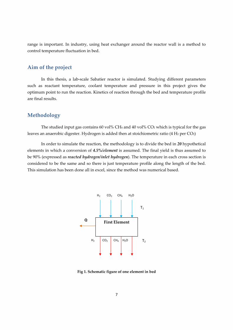
In order to simulate the reaction, the methodology is to divide the bed in 20 hypothetical elements in which a conversion of 4.5%/element is assumed. The final yield is thus assumed to be 90% (expressed as reacted hydrogen/inlet hydrogen). The temperature in each cross section is considered to be the same and so there is  just temperature profile along the length of the bed. This simulation has been done all in excel, since the method was numerical based. 

 

 

 

 

 

 

 

 

 

Fig 1. Schematic figure of one element in bed 

H2  CO2  CH4  H2O 

T1 

H2  CO2  CH4  H2O T2 

Q  First Element

8  

In fig 1, there is a schematic view of one element of the 20 ones in the reactor tube. As it is clear, the streams with temperature T1 and with different volumetric flows enter the element. The heat which  is produced  in  the reaction can either  increase  the  temperature of  the effluent stream  to  T2  or  be  released  from  the  wall  to  the  cooling  media.  In  reality  both  of  these mechanisms  happen  in  parallel,  but  in  our  calculations we  simulate  them  individually.  The results of the isothermal and the adiabatic simulation then can be compared with one another. 

As  reactor  tubes,  the  inner  diameter  of  35 mm was  chosen  since  this  is  a  standard diameter  that  is  easily  available  and  is used  in  laboratory  reactor. Tube  length up  to  6 m  is available and it seems logical to design the reactor for single pass. A load of 1.94 mmol/sec CO2 and 90% conversion was assumed for tube and 10 bar pressure was chosen. 

   

9  

1 Discussion and results 

1.1 Simulation and calculation data 

1.1.1 Input data  

There are  some  initial values used as  the basis of  calculations. These data were  taken mainly from Lunde work as the major source of information in this task. Based on Lunde paper on  modeling  and  simulation  of  Sabatier  reactor,  the  estimated  inlet  flow  in  atmospheric pressure is 0.638 ft3/min (18.1 lit/min) (Lunde 1974). This value could be changed in 10 atm case easily, so the values for volumetric flow rate of each component in influent become as in table 1. 

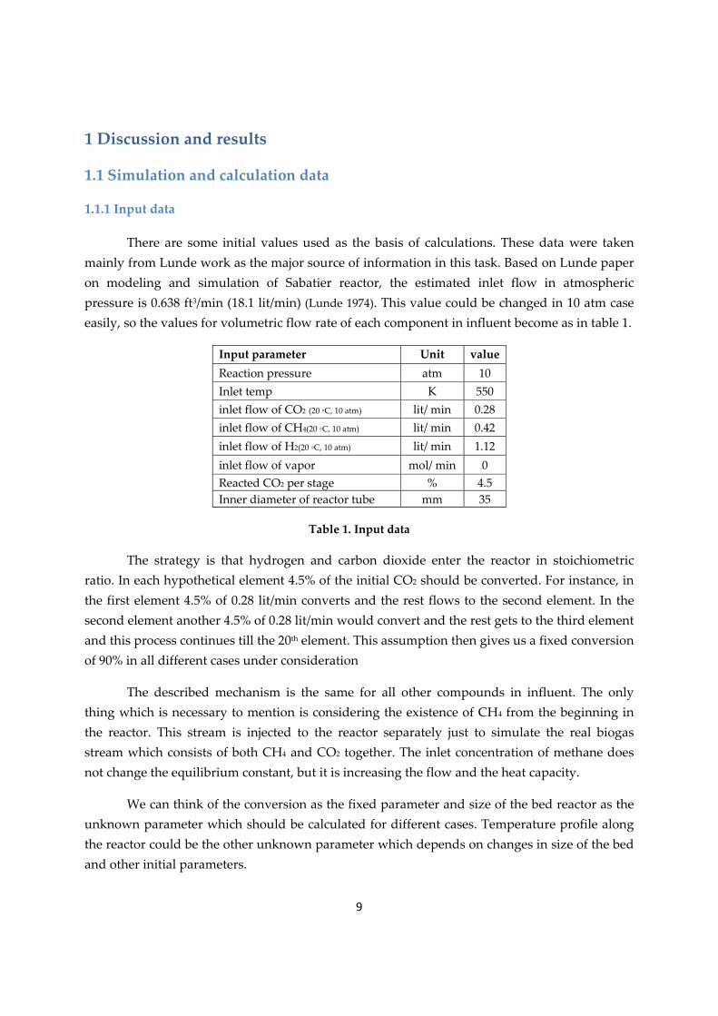
Input parameter  Unit  value Reaction pressure  atm  10 Inlet temp  K  550 inlet flow of CO2 (20 ◦C, 10 atm)  lit/ min  0.28 inlet flow of CH4(20 ◦C, 10 atm)  lit/ min  0.42 inlet flow of H2(20 ◦C, 10 atm)  lit/ min  1.12 inlet flow of vapor  mol/ min  0 Reacted CO2 per stage  %  4.5 Inner diameter of reactor tube   mm  35 

 

Table 1. Input data 

The  strategy  is  that  hydrogen  and  carbon  dioxide  enter  the  reactor  in  stoichiometric ratio. In each hypothetical element 4.5% of the initial CO2 should be converted. For instance, in the first element 4.5% of 0.28  lit/min converts and the rest flows to  the second element. In  the second element another 4.5% of 0.28 lit/min would convert and the rest gets to the third element and this process continues till the 20th element. This assumption then gives us a fixed conversion of 90% in all different cases under consideration 

The  described mechanism  is  the  same  for  all  other  compounds  in  influent.  The  only thing which is necessary to mention is considering the existence of CH4 from the beginning in the  reactor.  This  stream  is  injected  to  the  reactor  separately  just  to  simulate  the  real  biogas stream which consists of both CH4 and CO2 together. The  inlet concentration of methane does not change the equilibrium constant, but it is increasing the flow and the heat capacity.  

We can think of the conversion as the fixed parameter and size of the bed reactor as the unknown parameter which should be calculated for different cases. Temperature profile along the reactor could be the other unknown parameter which depends on changes in size of the bed and other initial parameters. 

10  

In order to use the correlations in different articles for further calculation it is needed to change  the  flow  rate unit  from  lit/min  to mol/min. This  is easily done by using  the  ideal gas equation. Pressure  term  in the correlation  is equal to 10 atm which  is the total pressure of  the system and temperature is equal to 293 K.  

1.1.2 Division of bed into 20 elements  

In  table 2,  there are molar changes along  the bed  from  top  to bottom. The  first row  in this  table  is  the  input  flow of  the whole  reactor and  first element as well, but  the other  rows could be interpreted as the outflow of the element which is mentioned in the same row of the table. As it is shown, the total number of moles is reducing through the reaction. This is because of  the non‐equimolar characteristics of  the  reaction. Also  the  relation between molar  flows of different components is based on stoichiometric ratio. 

No. of elements 

n CO2 (mmol/min) 

n H2 (mmol/min) 

n CH4 (mmol/min) 

delta CH4 (mmol/min) 

nH2O (mmol/min) 

ntot (mmol/min) 

0  116.45  465.8  174.7  0  0  756.95 

1  111.21  444.84  179.92  5.25  10.5  746.50 

2  106.00  424.00  185.16  10.50  21.00  736.16 

3  100.73  403.00  190.40  15.72  31.44  725.60 

4  95.50  382.00  195.64  21.00  41.92  715.06 

5  90.25  361.00  201.00  26.20  52.40  704.65 

6  85.00  340.00  206.12  31.44  63.00  694.12 

7  80.00  319.10  211.36  36.7  73.40  683.90 

8  74.53  298.11  216.60  41.92  83.85  673.10 

9  69.30  277.15  221.84  47.16  94.32  662.61 

10  64.05  256.20  227.10  52.40  104.80  652.15 

11  58.81  235.23  232.32  57.64  115.30  641.70 

12  53.56  214.30  237.56  62.88  125.80  631.122 

13  48.32  193.30  242.80  68.12  136.25  620.70 

14  43.08  172.35  248.04  73.36  146.73  610.20 

15  37.85  151.40  253.30  78.60  157.21  599.76 

16  32.60  130.42  258.50  84.00  167.70  589.22 

17  27.36  109.50  263.8  89.08  178.17  578.83 

18  22.12  88.50  269.00  94.32  188.67  568.30 

19  17.00  67.54  274.25  99.56  199.13  557.92 

20  11.65  46.60  279.50  104.80  209.61  547.40  

Table 2. Mole fractions in each element (4.5% conversion in each) 

11  

1.1.3 Cases for simulation  

In this report there are two main cases considered. The first case is the adiabatic one in which all  the generated heat  is used  to  increase  the  temperature of  the  flows downward and nothing  can be  released  to  the  surrounding. The  second  case  then  is known  as  the  real  case which happens  in reality. The attempt  in  this case  is  to control  temperature  in  the bed on  the constant  amount  by  cooling  the  bed  in  a  heat  exchanging mechanism with  a  coolant  flows around the reactor. 

1.1.4 Kinetic equation  

Emmett did a complete research on carbon dioxide methanation which was published as a book named “catalysis”. He believed  that  the methanation process can be described as  two consecutive reactions (Emmett 1951): 

                (a) 

      3           (b) 

Since  the  first  reaction  is  slow  at  the  used  reaction  temperature  (207‐371◦C)  and  the second  one  is more  rapid  than  the  (a), more  in  equilibrium  form,  then  there  is  no  carbon monoxide in the output stream. (Kester 1974) 

Knowing the real reactions which are happening helps finding the catalytic mechanism and then formulating a model for the reaction. Since the reaction is in gas phase and reversible, reaction rate is dependent both on partial pressure of reactants and products. Lunde has found a correlation for calculating this parameter (Lunde 1974). 

   (1) 

Lunde and Kester in the process of finding a well‐suited correlation for rate of reaction did some experiments in laboratory reactors. Through these tests, they could estimate values for k, Ea and n with a rather good liability. In their investigation the following values were found: 

k= 0.1769× 1010 Ea= 16.84 kcal/gmol (30.320 btu/lbmol)  n= 0.225  

They derived  these values  from  curves  and  lines of  experimental  results  in different H2/CO2 ratios and also in different temperatures. (Lunde, Peter J.,Kester, Frank L 1973)  

 

12  

1.1.5 Equilibrium considerations  

The rate of reaction  is also depending on the equilibrium constant (Ke ) and Ke  itself  is temperature  dependent.  The  extended  equation  for  equilibrium  constant  calculation  is  as following (Lunde, 1974): 

.

. . .                  (2) 

In  this  equation,  Tk  stands  for  Temperature  in Kelvin  unit.  This  equation  is  derived based on thermodynamic data by Wagman and et al in 1945 according to methods described by Brewer  and Pitzer  in  1961. The heat  capacities  that were used  in  this  equation derived  from Bureau of Mines Bulletins in 1949, 1950 and 1960 (Lunde, Peter J., Kester, Frank L. 1974) 

 

 

 

   

13  

1.2 Simulation result for the adiabatic case with interstage cooling  

In this case, it is assumed that the heat which is generated through the reaction in each element is not released from the reactor, but increases the temperature of the outflow instead. 

First of all it is needed to have some strategy for bed sizing, so then it could be modified or completed with  temperature and enthalpy considerations. The  following  steps are used  to calculate the length of bed: 

I. Calculating the rate of reaction by equation (1) II. Changing the unit atm./hr to mol/m3.min by simple using of ideal gas correlation III. Calculating volume of bed by dividing produced CH4 molar  flow  rate  in  each 

element with rate of reaction in that specific element. IV. Calculating length of each element by considering the fixed cross sectional area  V. The strategy in simulating this case is based on enthalpy changes along the bed.  

The  enthalpy  transformations  occur  because  of  temperature  increase  due  to  the exothermic nature of reaction. The total enthalpy is constant, but chemical enthalpy is converted to  thermal  enthalpy.  In  order  to  relate  the  enthalpy  of  components  to  temperature  changes, there are some polynomial correlations in different articles. Constants in these correlations are experimentally  determined  for  different  gases.  Frolov  and  et.al  (2009)  in  an  article  derived different experimental correlations for enthalpy calculations of real gases.  

The molar enthalpy for CO2 with reference temperature of 0 K in ideal‐gas case is given as follows in Frolov article: 

. . ∑ /         (3) 

In equation (3), θi  for CO2 has different values. θ1 = 3380 K, θ2 = 1995 K and θ3 = θ4=960 K. 

In the same article, there is another correlation which would be applied for the thermal enthalpy of H2 as an ideal gas. In this one the assumptions are the same as before and θ = 6323.26 K. 

. . /         (4) 

The given correlations are both for reactants, but in order to do the calculations for the adiabatic case it is needed to have functions for product enthalpies as well. For H2O, there is a correlation  in  the  same article as well;  therefore  the assumptions are nearly  similar with  two previous components. 

14  

. . . ∑ /   (5) 

In equation 5, the new parameter xi is just a simple θi to T ratio : ( xi = θi/T). For H2O the values for θi are as follows: θ1 = 5260.73 K, θ2 = 2294.37 K, θ3 = 5403.36 K. 

To calculate the thermal enthalpy for CH4 there is another type of polynomial which is given by Passut and Danner (1972). 

               (6) 

A,B,C,D,E and F are coefficients regarding to enthalpy in Btu/lb and temperature in ◦R . For CH4 the values for A to F are as following:  

A  =  ‐5.58114, B  =  0.564834, C  =  ‐0.282973  ×  10‐3, D  =  0.417399  ×  10‐6        E = ‐1.525576 × 10‐10, F = 1.958857 × 10‐14 

It is necessary to mention that since all the values in this report is in SI system, the enthalpy unit from equation (5) should be changed into SI 

Now  having  the  enthalpy  function  of  all  components  in  the  reaction,  the  calculations could be done properly and knowing the fact that in Sabatier reaction there is ‐165 kJ/mol produced CH4 heat production,  the  exit  temperature of  each  element  can be  calculated by  the  following equations. 

                (7) 

. %   (8) 

Based on equation (8), the value for Qgenerated is a fixed amount for all elements which in this case is equal to 14.4 W per element. In equation (7) then, the left side is the same as equation (8), the F values are changing through the bed from top to bottom and enthalpies are changing due to the temperature changes, as well. Hin is a function of Tin and Hout is Tout dependent. The output temperature of each element is the input one for the next element. The other point which is necessary to mention is to assume the element temperature equal to input flow temperature. For example, in element number 1, the input flow temperature is 550K and it is assumed that the reaction in this element happens in 550 K as well. 

In calculating the output temperature of each element, the temperature level increases to the point that the equilibrium conversion is reached in the middle of reactor and so the reaction could not go  further and get  to  the assumed conversion of 90%.  In  table 3  there are  results of adiabatic  simulation  on  temperature  and  enthalpy  aspects. As  it  is  clearly  shown  the  critical temperature happens somewhere around the 11thelement. The equilibrium conversion (Xe) in this 

15  

case  is  47%  which  is  happening  somewhere  around  the  11th  element.  The  highest  possible temperature which could be reached in adiabatic trial is 907.4469 K and in temperatures higher than that, equation (1) gets to zero or negative values and so it means that there could not be any reaction  in  temperatures higher  than  this. Therefore  the 12th element and so  forth ones do not play any role in this reaction! 

Next step is to size each element and the whole bed respectively. The strategy has been already  discussed,  but  there  is  some more  to  consider  and  it  is  about  the  steep  increase  of reaction rate by temperature rise. This fact then results in a very small volume for each element and so almost 50% conversion happens just in the first 1cm of the bed! 

In table 3, there are calculation results of the 11 elements which reaction happens in them. It  is  clear  enough  that  the volume of  each  element  is decreasing  sharply  and  also  the  rate  of reaction is increasing in big steps even though the conversion is the fixed value of 4.5% in each element. 

The graphical view of results in table 4 and 5 are given in following graphs. In figure 2, there  are  changes of yield  and  equilibrium  conversion  changes  through  the bed.  It  is  clearly shown  that  in conversion around 50%  the equilibrium and yield curve  intercept one another. This means  that  the reaction gets  to equilibrium at  this point and so  it cannot go  further and increase the conversion of the reactants. 

 

No. of elements 

Tgas K  Yield  H(kW) r CO2 

(mol/lit.hr) L (mm) 

1  550  0.045  0.222  43.09  7.30 2  586.4  0.09  0.237  100.72  3.12 3  621.6  0.135  0.251  204.86  1.53 4  658.3  0.18  0.265  389.40  0.81 5  696  0.225  0.281  687.52  0.46 6  731.5  0.27  0.295  1077.38  0.29 7  767.1  0.315  0.310  1561.98  0.20 8  803.6  0.36  0.325  2095.01  0.15 9  838.6  0.405  0.340  2480.90  0.13 10  873.2  0.45  0.353  2497.60  0.126 11  907.4  0.495  0.368  1764.25  0.18 12  941.3  0.54  0.382  ‐266.58  ‐1.18 

 

Table 3. Temperature changes along the bed and reactor sizing in the adiabatic case 

16  

14.30, 0.47

0

0.2

0.4

0.6

0.8

1

1.2

0 5 10 15 20

Conversion

Length of the bed(mm)

yield equilibriumconversion

In figure 3 then, there are the changes in temperature through bed. The sudden increase in temperature in the very beginning of the reactor is something which is obvious in this figure.  

 

Fig 2. Conversion versus length of the bed in the adiabatic case 

There  is another point  in  figure 3 which shows  the point which  the curve  is somehow turning  back  to  the  left. This  is  just  to  show  that  the  reaction  gets  to  equilibrium  and  stops progressing further more. 

In  adiabatic  case  the  temperature  increase  occurs which  has  negative  impact  on  the efficiency  and  catalyst  activity,  therefore  engineers  thought of  some  solutions;  an  Inter  stage cooling system which is processing after each two or three elements.  

17  

907.45

0100200300400500600700800900

1000

0 2 4 6 8 10 12 14 16

tempe

rature (K

)

length of the bed (mm)

adiabatic case

 

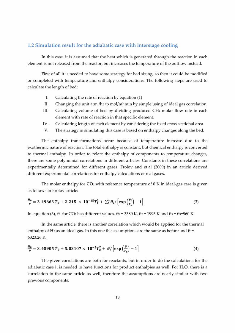
Fig 2. Temperature versus length of the bed in the adiabatic case 

 

 

 

Fig 3. Reactor staging with interstage cooling (Fogler 2006) 

Regarding  figure 3 which  is a  schematic view of  the “interstage cooling”,  the  influent gets heated  through the exothermic reaction. This flow then  is needed to be cooled down  in a separate  heat  exchanger  to  keep  the  reaction  progressing  in  the  next  adiabatic  section.  This cooling continues till getting to the specific needed conversion. 

 

 

 

 

 

 

 

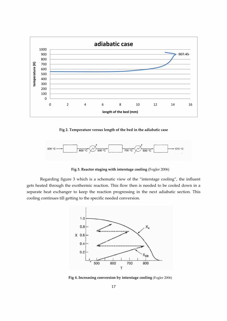
Fig 4. Increasing conversion by interstage cooling (Fogler 2006) 

18  

As  it  is  shown  in  figure 4,  the  interstage  cooling  increases  the  conversion  in a  certain temperature range by preventing the reaction to get to equilibrium conversion. 

In  the current study  the reaction  is highly exothermic, so  in  the adiabatic case without any interstage cooling the reaction gets to equilibrium conversion somewhere in the middle of the reactor which stops reaction to move forward more. This phenomenon could be controlled then by applying a strategy of intercooling. 

 

Fig 5. Increasing conversion by interstage cooling 

Referred to Lunde and Kester work which was published on 1974 and also their separate efforts on this, there is a suitable temperature range for carbon dioxide methanation from 400‐700°F (200‐371 °C or 473‐644 K). Sticking to this temperature range should be always considered for temperature controlling. (Lunde, Peter J.,Kester, Frank L 1973) (Kester 1974) 

In  figure  5  the  interstage  cooling mechanism  is  shown  by  black  arrows  and  dashes which could be interpreted as using 5 heat exchangers in the reactor. In other words it is needed to divide  the  reactor  in 6  reactions which are working  in  series and  the  reactant  flow passes through the heat exchangers during the reaction period.  

Based  on  figure  5,  6  reactors  are  needed  for  this  type  of  operating  the  reaction.  The sizing parameters of these reactors are the same as before. The inner diameter of all of them is 35 mm, but their lengths are varying which is given in table 4. 

0

0.2

0.4

0.6

0.8

1

1.2

550 650 750 850 950 1050

Conversion

Temperature, K

equilibrium conversionyield

19  

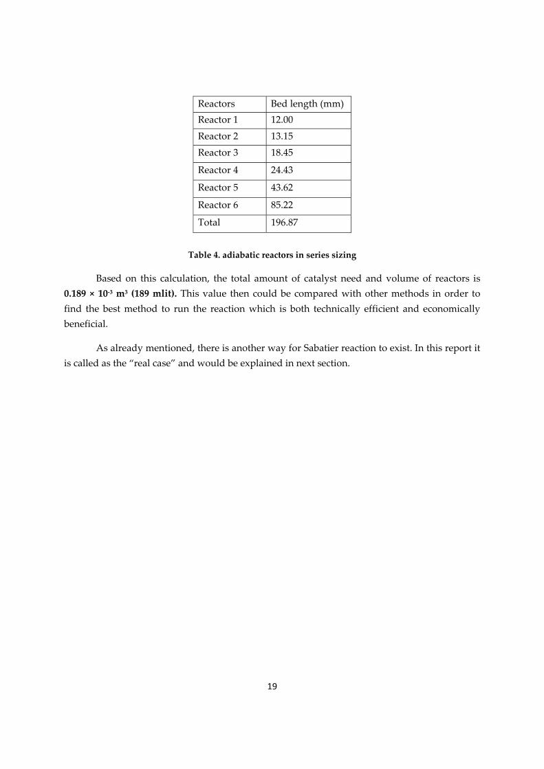
Reactors  Bed length (mm) Reactor 1  12.00 

Reactor 2  13.15 

Reactor 3  18.45 

Reactor 4  24.43 

Reactor 5  43.62 

Reactor 6  85.22 

Total  196.87  

Table 4. adiabatic reactors in series sizing 

Based on  this  calculation,  the  total amount of  catalyst need and volume of  reactors  is 0.189 × 10‐3 m3  (189 mlit). This value  then could be compared with other methods  in order  to find  the best method  to  run  the  reaction which  is both  technically efficient and economically beneficial.  

As already mentioned, there is another way for Sabatier reaction to exist. In this report it is called as the “real case” and would be explained in next section. 

   

20  

1.3 Results of Real case 

1.3.1 Theoretical formulation  

Next strategy for simulating the reactor is to consider a cooling system around it. In this way of thinking, the heat which is produced through reaction could be released and so keep the temperature on a suitable level. 

The energy balance for one element considering both exothermic reaction and a coolant flow around the reactor wall is as follows: 

                (9) 

This  is  almost  the  same  as  equation  (8), but with  an  additional parameter which  is  a symbol for the amount of heat that is released to coolant. Qreleased should be calculated based on heat transfer through reactor wall and coolant media.  

 

 

 

 

 

 

 

 

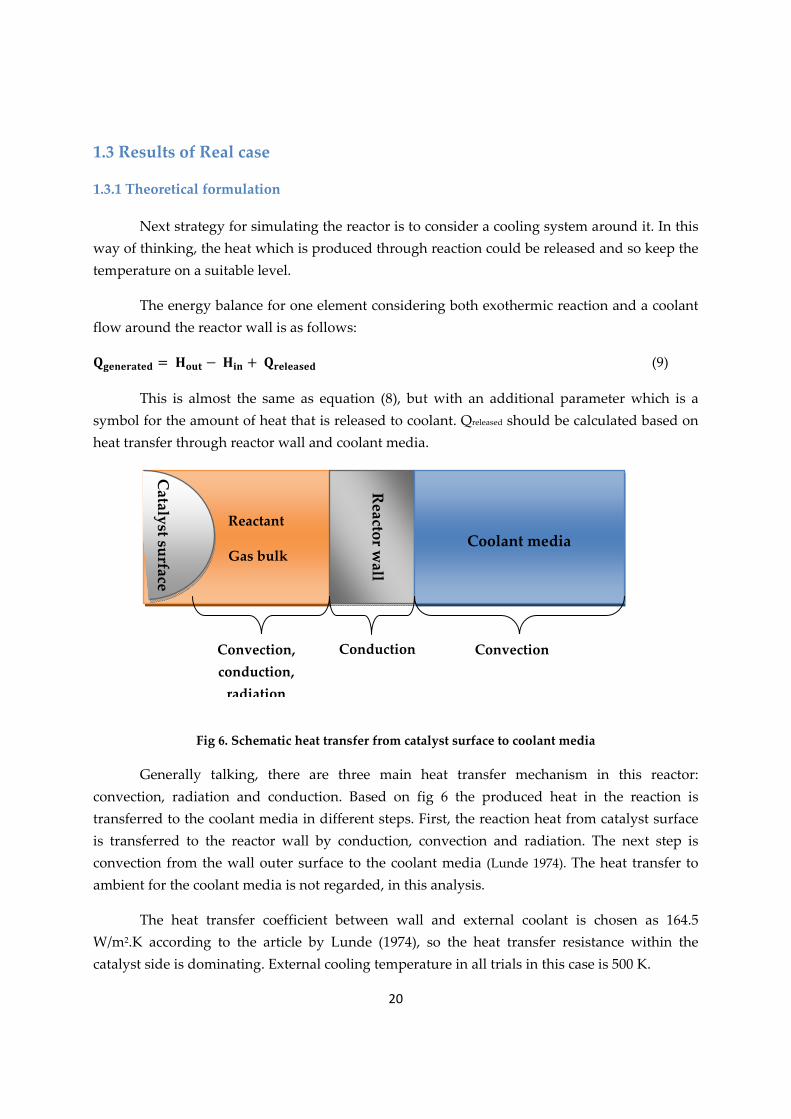
Fig 6. Schematic heat transfer from catalyst surface to coolant media 

Generally  talking,  there  are  three  main  heat  transfer  mechanism  in  this  reactor: convection,  radiation  and  conduction.  Based  on  fig  6  the  produced  heat  in  the  reaction  is transferred to the coolant media in different steps. First, the reaction heat from catalyst surface is  transferred  to  the  reactor wall  by  conduction,  convection  and  radiation.  The  next  step  is convection  from  the wall outer surface  to  the coolant media  (Lunde 1974). The heat  transfer  to ambient for the coolant media is not regarded, in this analysis.  

The  heat  transfer  coefficient  between  wall  and  external  coolant  is  chosen  as  164.5 W/m2.K  according  to  the  article  by  Lunde  (1974),  so  the  heat  transfer  resistance within  the catalyst side is dominating. External cooling temperature in all trials in this case is 500 K. 

                 

                     Reactant  

                     Gas bulk 

        

Catalyst surface

Reactor w

all 

 

Coolant media 

Convection, conduction, radiation

Conduction Convection

21  

Regarding  the  existence  of  a  cooling  system,  the  released  heat  should  be  calculated through some correlations directly. It could be assumed that heat transfer mechanism which is more  dominant  in  this  case  is  the  convection  from  the  gas  to  the wall  because  it  could  be assumed that there is a same temperature in all parts of the wall and also the fixed temperature in all cooling media. These assumptions then can result in following equation for Qreleased . 

, ,              (10) 

In this equation, the heat transfer coefficient hwall is considered as a known value and the reference for it is the article about Sabatie reactor modeling and simulation by Lunde (1974). In this article the value for hw is 14 Btu/hr.ft2.◦F which is equivalent to 79.5 W/m2.K. The parameter A  then  is heat  transfer area which  is  the area of  the element wall exposed  to  the coolant and could be calculated as follows: 

                      (11) 

On  the other hand  it  is  important  to have  some  idea about  the cooling mechanism as well. The heat exchanging process around the reactor wall could be either co‐current or counter‐current. The difference  between  these  two  categories  could  be  seen  qualitatively  in different literatures and references. For example there are some typical graphs in “Elements of chemical reaction engineering” by Fogler which is about heat effects in PFR/PBR s.  

 

 

 

 

 

 

 

  

(a)                                   (b) 

Fig 7. Schematic graphs for exothermic reactions with cooling system (a).The exothermic reaction with counter‐current cooling,(b) The exothermic co‐current exchanger (Fogler 2006) 

 

22  

1.3.2 Analytical calculations and results  

Considering  all  formulations  in  section  1.3.1,  there  should  be  some  analysis  prior  to simulation. Actually  size of each element  is one of  the  important parameters  since  it directly affects  the  amount  of  heat  release  through  reactor wall.  Therefore,  element  length  has  key influence on the gases temperature flowing through the bed. 

If the reactor should not be overheated, it is needed to have enough heat transfer area to let the heat be released. To provide cooling surface, using some inert packings such as catalyst support material  are definitely  needed. Therefore  in  each  element  the  inert  packings  can  be added to catalyst packings and to increase the length of element for achieving sufficient cooling. 

In this analysis, there are two different lengths, active length and physical length. The active  length  is  just  referred  to  the  catalyst  amount,  but  physical  length  is  the  total  size  of element which is the combination of both active catalysts and inert packings. In figure 8, there is the schematic picture of what is thought to be done. 

To explain the strategy it could be started with describing figure 8 in detail. The process starts  at  the  top  of  reactor with  the  first  element.  The  active  length  of  this  element  has  the smallest one among  the other  elements  if  the  temperature needed  to be  controlled  in a  fixed value.  In  the  top  elements which  the  conversion  is  around  50%,  the  cooling  process  is  rate determining and the more cooling happens the better rate controlling could be done. Therefore in order to eliminate temperature increase it is needed to increase heat transfer area. This is the reason for two different sizing (Active and physical lengths) for top elements of the reactor  

On the other hand, the more reactants go further down in reactor the less would be the impact  of  cooling  for  rate  determining  and  instead  the  reaction  itself  would  be  the  rate determining parameter. In this strategy for the last two elements in which the reactants have the least  concentration,  full active  size  is  considered.  In other words,  these  final elements do not have any inert packings and are filled only by active catalysts.  

According  to what has been mentioned above,  the most  important part of  the  reactor design is the last two elements. They have the major load of catalyst in them and so in order to optimize technically and economically it is needed to optimize the amount of catalysts needed for the whole process. 

If the reactor operates in high temperature, then the rate of the reaction increases and the active  length would  be  reduced  so  the  higher  temperature  gets  the  less  amount  of  catalyst would be needed.  

 

23  

 

 

 

 

 

 

 

 

 

 

 

Fig 8. Schematic picture of the strategy in simulating real case 

On  the  other  hand,  it  is  important  to  consider  the  negative  impacts  of  very  high temperature.  First  of  all  the  reaction  cannot  go  forward  in  high  temperatures  and  the equilibrium occurs earlier  than  the expected conversion.  In equilibrium conditions, as already discussed, there are reactions at both directions and it could be interpreted as “reaction stops”. The other side effect is sintering and deactivation of catalysts. Sintering happens in the case that catalyst has too long exposure to high temperature and the support gets soft and flows, so the active  pores  of  catalyst  get  narrow  and  close  inside  catalyst  pellet  (Fogler  2006).  At  high temperatures  the  catalysts are needed  to be  regenerated or  renewed  earlier and  this  is a  fact which should be thought of in designing the reaction conditions. 

Regarding  stated  parameters,  there  should  be  an  operating  range  for  the  reaction temperature in which there is definitely one point which could cover all aspects of concern. In order to determine this specific point, calculations should be done for the whole bed, but before that the operating range should be derived by focusing on last two elements. The procedure is based  on  trial  and  error  method.  Sizing  of  the  last  element  would  be  done  in  different temperatures and X‐Y coordinance of temperature‐size curve would be saved then. The initial temperature in this trial is 550 K in the case that coolant has the fixed temperature of 500 K in all the tests. The results are shown in table 6 and figure 8 respectively. 

1st element physical length 1st element active size 

T °K 

2nd element physical length 2nd element active size 

T °K 

3rd element physical length 3rd element active size 

T °K 

20th element physical length 20th element active size 

T °K 

T °K

24  

 

Initial temperature 

(K) 

Last element temperature (K) 

Last element size (mm) 

550  537  104.57 560  550.85  76.61 600  606  27.72 650  664.5  23.74 656  670.86  27.97 662  677.11  37.32 670  685.15  95.94 675  690.06  ‐354.88 700  709  ‐11.2 

 

Table 5. Different trials to find operating temperature range for the last element 

 

Fig 9. Changes on last element length by operating temperature 

According  to  table  5  and  figure  9,  the  temperature  increase  would  result  in  length decrease. This temperature rise change its’ effect more than an amount and also from a level on there is no more reaction happening. This fact could be viewed in the negative values appeared in “last element size” column in table 6 and points on the right side of the red line in figure 9. 

Regarding these results, the smallest size for the last element would be resulted in 650K as the initial temperature which has a bit of increase before the last element and gets to 664.5 K. The question is then if 650K is the optimum temperature for running the reactor in? In order to find a proper answer for this one, it is needed to consider some other facts as well. In following 

25  

pages  there are simulation  results of 3 different applicable  temperatures which  then could be analyzed to find the optimum temperature. 

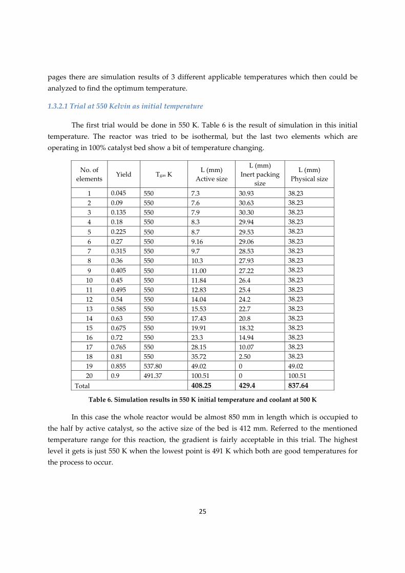
1.3.2.1 Trial at 550 Kelvin as initial temperature  

The first  trial would be done  in 550 K. Table 6  is  the result of simulation  in  this  initial temperature.  The  reactor  was  tried  to  be  isothermal,  but  the  last  two  elements  which  are operating in 100% catalyst bed show a bit of temperature changing. 

No. of elements 

Yield  Tgas K L (mm) 

Active size 

L (mm) Inert packing 

size 

L (mm) Physical size 

1  0.045  550  7.3  30.93  38.23 2  0.09  550  7.6  30.63  38.23 3  0.135  550  7.9  30.30  38.23 4  0.18  550  8.3  29.94  38.23 5  0.225  550  8.7  29.53  38.23 6  0.27  550  9.16  29.06  38.23 7  0.315  550  9.7  28.53  38.23 8  0.36  550  10.3  27.93  38.23 9  0.405  550  11.00  27.22  38.23 10  0.45  550  11.84  26.4  38.23 11  0.495  550  12.83  25.4  38.23 12  0.54  550  14.04  24.2  38.23 13  0.585  550  15.53  22.7  38.23 14  0.63  550  17.43  20.8  38.23 15  0.675  550  19.91  18.32  38.23 16  0.72  550  23.3  14.94  38.23 17  0.765  550  28.15  10.07  38.23 18  0.81  550  35.72  2.50  38.23 19  0.855  537.80  49.02  0  49.02 20  0.9  491.37  100.51  0  100.51 

Total  408.25  429.4  837.64  

Table 6. Simulation results in 550 K initial temperature and coolant at 500 K 

In this case  the whole reactor would be almost 850 mm  in  length which  is occupied to the half by active catalyst, so  the active size of  the bed  is 412 mm. Referred  to  the mentioned temperature  range  for  this  reaction,  the gradient  is  fairly  acceptable  in  this  trial. The highest level it gets is just 550 K when the lowest point is 491 K which both are good temperatures for the process to occur. 

 

26  

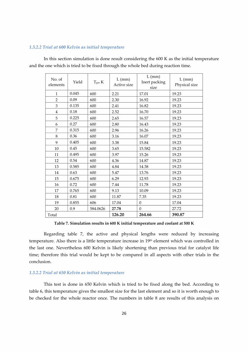
1.3.2.2 Trial at 600 Kelvin as initial temperature  

In this section simulation is done result considering the 600 K as the initial temperature and the one which is tried to be fixed through the whole bed during reaction time. 

No. of elements 

Yield  Tgas K L (mm) 

Active size 

L (mm) Inert packing 

size 

L (mm) Physical size 

1  0.045  600  2.21  17.01  19.23 2  0.09  600  2.30  16.92  19.23 3  0.135  600  2.41  16.82  19.23 4  0.18  600  2.52  16.70  19.23 5  0.225  600  2.65  16.57  19.23 6  0.27  600  2.80 16.43 19.23 7  0.315  600  2.96  16.26  19.23 8  0.36  600  3.16  16.07  19.23 9  0.405  600  3.38  15.84  19.23 10  0.45  600  3.65  15.582  19.23 11  0.495  600  3.97  15.26  19.23 12  0.54  600  4.36 14.87 19.23 13  0.585  600  4.84  14.38  19.23 14  0.63  600  5.47  13.76  19.23 15  0.675  600  6.29  12.93  19.23 16  0.72  600  7.44  11.78  19.23 17  0.765  600  9.13  10.09  19.23 18  0.81  600  11.87  7.35  19.23 19  0.855  606  17.04  0  17.04 20  0.9  584.0626  27.78  0  27.72 

Total  126.20 264.66 390.87  

Table 7. Simulation results in 600 K initial temperature and coolant at 500 K 

Regarding  table  7,  the  active  and  physical  lengths  were  reduced  by  increasing temperature. Also there is a little temperature increase in 19th element which was controlled in the  last  one. Nevertheless  600 Kelvin  is  likely  shortening  than previous  trial  for  catalyst  life time;  therefore  this  trial would be kept  to be  compared  in all aspects with other  trials  in  the conclusion. 

1.3.2.2 Trial at 650 Kelvin as initial temperature  

This  test  is done  in 650 Kelvin which  is  tried  to be  fixed along  the bed. According  to table 6, this temperature gives the smallest size for the last element and so it is worth enough to be  checked  for  the whole  reactor once. The numbers  in  table 8 are  results of  this analysis on 

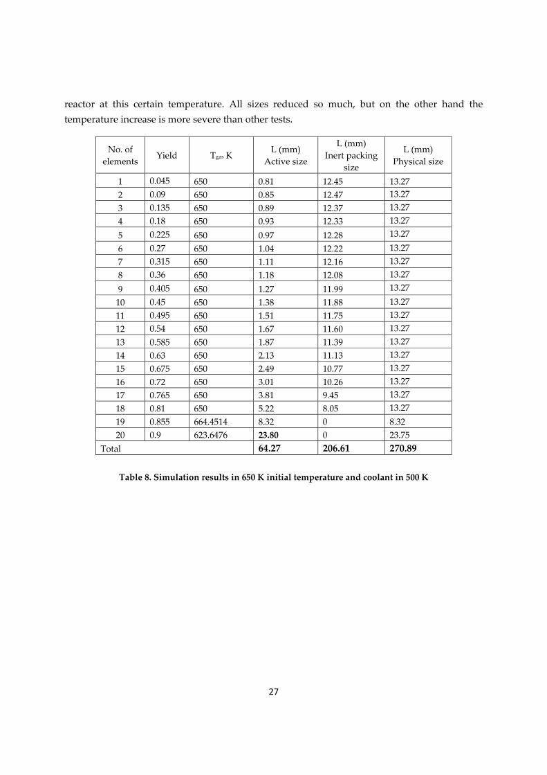
27  

reactor  at  this  certain  temperature.  All  sizes  reduced  so much,  but  on  the  other  hand  the temperature increase is more severe than other tests. 

No. of elements  Yield  Tgas K 

L (mm) Active size 

L (mm) Inert packing 

size 

L (mm) Physical size 

1  0.045  650  0.81  12.45  13.27 2  0.09  650  0.85  12.47  13.27 3  0.135  650  0.89 12.37 13.27 4  0.18  650  0.93  12.33  13.27 5  0.225  650  0.97  12.28  13.27 6  0.27  650  1.04 12.22 13.27 7  0.315  650  1.11  12.16  13.27 8  0.36  650  1.18  12.08  13.27 9  0.405  650  1.27  11.99  13.27 10  0.45  650  1.38  11.88  13.27 11  0.495  650  1.51  11.75  13.27 12  0.54  650  1.67 11.60 13.27 13  0.585  650  1.87  11.39  13.27 14  0.63  650  2.13  11.13  13.27 15  0.675  650  2.49  10.77  13.27 16  0.72  650  3.01  10.26  13.27 17  0.765  650  3.81  9.45  13.27 18  0.81  650  5.22  8.05  13.27 19  0.855  664.4514  8.32  0  8.32 20  0.9  623.6476  23.80  0  23.75 

Total  64.27  206.61  270.89  

Table 8. Simulation results in 650 K initial temperature and coolant in 500 K 

 

   

28  

1.4Comparison of adiabatic case with isothermal case  

Regarding all the challenges about the adiabatic and isothermal cases, each of them has some cons and pros. Adiabatic method  is  technically possible, but  there are some economical and operational concerns which make it a bit difficult.  

i. Maintenance  cost:  Using  small  heat  exchangers  instead  of  one  big  cooling system  around  the  whole  reactor  increases  the  risk  of  operation  and maintenance. They have  their piping systems each which add up  to controlling systems  of  the  process  on  the  plant  and  make  the  whole  package  more complicated than isothermal case.   

ii. Occupied space: The other point  is about size of the whole “reaction package”. The adiabatic case consists of five heat exchangers and six small reactors which surely  occupy more  space  than  one big  reactor with  one heat  exchanger. This makes the method critical in the situation with “limited space” issue. 

 iii. Energy cost: Running five small heat exchangers needs more energy  than a big 

one. This is categorized in economical concerns about adiabatic method.  iv. Operation cost: The adiabatic case consumes more catalyst  in comparison with 

almost all of the runs in isothermal case. This is considered surely in economical concerns. Also  in  the adiabatic method each reactor works  in high  temperature which can reduce the lifetime of catalyst after some hours of operating, when in isothermal case the temperature control in a fairly low temperature keeps the life time span of catalyst in a better condition. This parameter leads to more catalyst regenerating or changing during  the  life  time of  the  reactor which has  its own cost effects as well. 

On the other hand adiabatic case has some advantages compared to the isothermal case. For example, the reaction could go on even  if one or more reactors do not work. Of course  in this situation the final conversion is not satisfying, but anyhow the reaction does not shutdown completely. This  is  the  same with heat exchangers. They  could  cover one another  role  in  the system  if there would be a fault  in any of them, since  in  isothermal case there is  just one heat exchanger. 

In order  to  increase  the possibility  of using  adiabatic method,  there  is  a modification which could be done. This system is designed more to reduce the number of reactors and heat exchangers in series, therefore it consists of a big reactor  instead of first 5 ones, and one small 

29  

reactor as  the  last one. The amount of  conversion  in  this  system  is  the  same as  conventional adiabatic  and  also  the  temperature  limit  for  catalyst  activity  is  considered  similar  to  the adiabatic method. 

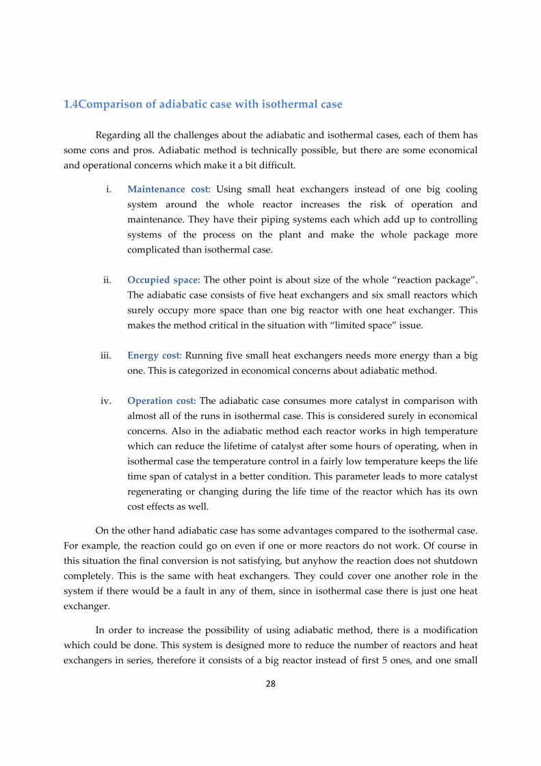
The mechanism  in modified  adiabatic  system,  as  in  figure  9,  is  that  some part  of  the cooled  product  stream  would  be  recycled  to  the  entrance  of  the  reactor.  This  would  help converting of influent before entering to the reactor to some extent. 

 

Fig 10. Modified adiabatic method 

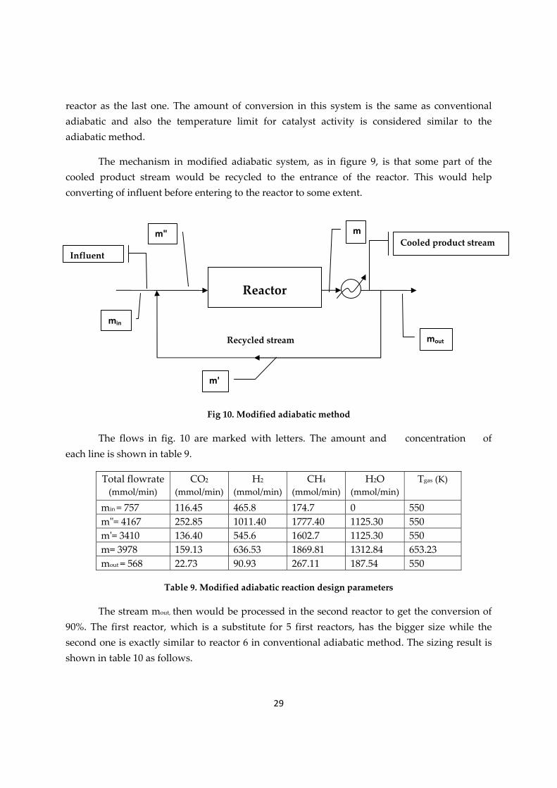
The  flows  in  fig.  10  are marked with  letters. The  amount  and  concentration  of each line is shown in table 9.  

Total flowrate (mmol/min) 

CO2 (mmol/min) 

H2 (mmol/min)

CH4 (mmol/min)

H2O (mmol/min) 

Tgas (K) 

min = 757  116.45  465.8  174.7  0  550 mʺ= 4167  252.85  1011.40  1777.40  1125.30  550 mʹ= 3410  136.40  545.6  1602.7  1125.30  550 m= 3978  159.13  636.53  1869.81  1312.84  653.23 mout = 568  22.73  90.93  267.11  187.54  550 

 

Table 9. Modified adiabatic reaction design parameters 

The stream mout, then would be processed in the second reactor to get the conversion of 90%. The  first  reactor, which  is a  substitute  for 5  first  reactors, has  the bigger  size while  the second one is exactly similar to reactor 6 in conventional adiabatic method. The sizing result is shown in table 10 as follows. 

Recycled stream 

Cooled product stream Influent 

Reactor 

m

m' 

m" 

min 

mout 

30  

 

 

 

 

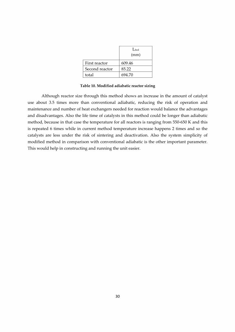
Table 10. Modified adiabatic reactor sizing 

Although reactor size through this method shows an increase in the amount of catalyst use  about  3.5  times  more  than  conventional  adiabatic,  reducing  the  risk  of  operation  and maintenance and number of heat exchangers needed for reaction would balance the advantages and disadvantages. Also the life time of catalysts in this method could be longer than adiabatic method, because in that case the temperature for all reactors is ranging from 550‐650 K and this is repeated 6  times while  in current method  temperature  increase happens 2  times and so  the catalysts  are  less  under  the  risk  of  sintering  and deactivation. Also  the  system  simplicity  of modified method in comparison with conventional adiabatic is the other important parameter. This would help in constructing and running the unit easier. 

   

  Lbed 

(mm) 

First reactor  609.46 Second reactor  85.22 total  694.70 

31  

2 Conclusion  

The present use of Sabatier  reaction  is CO2 elimination  in syngas  for ammonia plants. This  reaction  can  increase  the  efficiency  of  biogas  industry  on methane  production.  In  this report  the  focus  is more  on  temperature  controlling  of  this  system  and  optimizing different possible methods for running the reactor. 

Considering  all  results,  discussions  and  analyses  in  this  report  and  according  to  the comparison  of  adiabatic  reactor  with  the  isothermal  one,  it  is  clear  now  that  running  the reaction in isothermal condition is more beneficial and optimized than conventional adiabatic. It is also considerable that for a small laboratory reactor a single tube that combines reaction and cooling  surfaces  is much  cheaper and easier  to  run  than  six adiabatic beds and  five  separate coolers while  for  a  large  reactor with  a  large  cooling  demand  it may  be more  economic  to choose interstage coolers and adiabatic reactor sections.  

Even though applying some changes in adiabatic run, would lead us to a commercially feasible  method  which  could  be  competitive  with  isothermal  method  to  some  extent.  In modified adiabatic method, construction and maintenance is less complicated and costly while the amount of active catalyst is a bit more than isothermal case. On the other hand, up scaling these cases 10,000 times than the lab scale adds some extra considerations and points to analyze which would  be more  important  than  the  amount  of  active  catalyst use. The possibilities  of system upgrading, temperature controlling, substituting deactivated catalysts with active ones, constructing  easily  the plant  from  scratch, are  some parameters which make  the  choice a bit difficult.  

Since all these parameters have their own effect and cost to the total observation of the system,  selecting  the  best  one  is  so  dependent  and  needs  different  detail  designs  and economical calculations. 

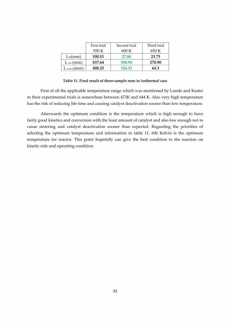
Regarding  all  above,  for  the  lab  scale  design  there  is  less  doubt  of  selecting  the isothermal run. This method should be optimized and the best condition would be selected to operate  the  reactor on  that.  In  table  12  there  are  results of  isothermal  runs  in  three different temperatures. The sample runs are  in 550 K, 600 K and 650 K respectively. There are also  the length  of  final  element,  total  physical  length  and  total  active  length  in  table  11.  The more temperature  increases  the  shorter  would  be  these  lengths  for  reactor,  but  the  optimum temperature is not the highest possible one.  

 

 

32  

 

 

 

 

Table 11. Final result of three‐sample runs in isothermal case 

First of all the applicable temperature range which was mentioned by Lunde and Kester in their experimental trials is somewhere between 473K and 644 K. Also very high temperature has the risk of reducing life time and causing catalyst deactivation sooner than low temperature.  

Afterwards  the  optimum  condition  is  the  temperature which  is  high  enough  to  have fairly good kinetics and conversion with the least amount of catalyst and also low enough not to cause  sintering  and  catalyst  deactivation  sooner  than  expected.  Regarding  the  priorities  of selecting  the  optimum  temperature  and  information  in  table  11,  600 Kelvin  is  the  optimum temperature  for  reactor.  This  point  hopefully  can  give  the  best  condition  to  the  reaction  on kinetic side and operating condition. 

 

 

   

  First trial 550 K 

Second trial 600 K 

Third trial  650 K 

L20(mm)  100.51  27.80  23.75 L tot (mm)  837.64  390.90  270.90 L active(mm)  408.25  126.21  64.3 

33  

Bibliography Emmett, PH 1951, Catalysis, Reinhold, New York. 

Fogler, HS 2006, Elements of chemical reaction engineering, 4th edn, Pearson education, United state. 

Frolov, S.M., Kuznetsov, N.M., Krueger, C 2009, ʹ Real‐gas properties of n‐alkanes O2,N2,H2O,CO,CO2 and H2 for diesel engine operation conditionsʹ, Russian journal of physical chemistry B, vol 3, no. 8, pp. 1191‐1252. 

Kester, FL 1974, ʹHydrogenation of carbon dioxide over a supported Ruthenium catalystʹ, Am Chem Soc, Div Fuel Chem, vol 19, no. 1, pp. 146 ‐156. 

Lunde, PJ 1974, ʹModeling, simulation. and operation of a Sabatier Reactorʹ, Industrial Engineering Chemical Process Design Develop., vol 13, no. 3, pp. 226‐233. 

Lunde, Peter J., Kester, Frank L. 1974, ʹ Carbon dioxide methanation on a Ruthenium catalystʹ, Industrial Engineering Chemical Process Design Develop., vol 13, no. 1, pp. 27‐33. 

Lunde, Peter J.,Kester, Frank L 1973, ʹRates of Methane formation from carbon dioxide and hydrogen over a ruthenium catalystʹ, Journal of catalysis, no. 30, pp. 423‐429. 

Passut, Charles A., Danner, Ronaldo P. 1972, ʹCorrelation of ideal gas enthalpy, heat capacity and entropyʹ, Industrial Engineering Chemical Process Design Develop., vol 11, no. 4, pp. 543‐544. 

Taglia P.G, P 2010, ʹBiogas: rethinking the mid west’s potentialʹ, clean Wisconsin. 

Violeta Bescós, LCSC 2008, ʹIntegration of synthetic methane into the existing biogas production of Henriksdalʹ, Report for the design course, p. 3.