Simulating Wireless Sensor Networks with OMNeT++users.cis.fiu.edu/~iyengar/publication/J-(2005...to...
25
LSU Simulator, Version 1, 01/24/2005 Simulating Wireless Sensor Networks with OMNeT++ C. Mallanda, A. Suri, V. Kunchakarra, S.S. Iyengar*, R. Kannan* and A. Durresi Sensor Network Research Group, Department of Computer Science, Louisiana State University, Baton Rouge, LA. [email protected], [email protected], [email protected], {iyengar,rkannan,durresi}@csc.lsu.edu S. Sastry The University of Akron, Akron, Ohio. [email protected] _________________________ * This work was supported in part by NSF-ITR under IIS-0312632 and IIS-0329738 and DARPA/AFRL grant #F30602-02-1-0198.
Transcript of Simulating Wireless Sensor Networks with OMNeT++users.cis.fiu.edu/~iyengar/publication/J-(2005...to...

LSU Simulator, Version 1, 01/24/2005
Simulating Wireless Sensor Networks with OMNeT++
C. Mallanda, A. Suri, V. Kunchakarra, S.S. Iyengar*, R. Kannan* and A. Durresi
Sensor Network Research Group, Department of Computer Science,
Louisiana State University, Baton Rouge, LA. [email protected], [email protected], [email protected],
{iyengar,rkannan,durresi}@csc.lsu.edu
S. Sastry
The University of Akron, Akron, Ohio. [email protected]
_________________________
* This work was supported in part by NSF-ITR under IIS-0312632 and IIS-0329738 and DARPA/AFRL grant #F30602-02-1-0198.

Abstract: Wireless sensor networks have the potential to become significant subsystems of engineering
applications. Before relegating important and safety-critical tasks to such subsystems, it is necessary to
understand the dynamic behavior of these subsystems in simulation environments. There is an urgent need
to develop simulation platforms that are useful to explore both the networking issues and the distributed
computing aspects of wireless sensor networks. Current efforts to simulating wireless sensor networks
largely focus on the networking issues. These approaches use well-known network simulation tools that are
difficult to extend to explore distributed computing issues.
Discrete-event simulation is a trusted platform for modeling and simulating a variety of systems.
We report results obtained from a new simulator for wireless sensor networks networks that is based on the
discrete event simulation framework called OMNeT++. Work is underway to develop a simulation
platform that allows developers and researchers to investigate topological, phenomenological, networking,
robustness and scaling issues related to wireless sensor networks. As a first step, we have developed
simulations for the 802.11 MAC and the well-known sensor network protocol called Directed Diffusion.
We demonstrate the performance of our simulator by comparing its performance to that of the well-known
simulator ns2. Our results indicate that our simulator executes at least an order of magnitude faster than
NS-2 and makes more efficient use of the available memory. The ease of modifying the sensor network
and scalability, which is defined as the number of nodes that can be simulated, are two distinguishing
features of our simulator.
Index Terms
Sensor Network, Performance Evaluation, Simulation
1. Introduction
Wireless Sensor Networks (WSN) [2] comprises of numerous tiny sensors that are deployed in
spatially distributed terrain. These sensors are endowed with small amount of computing and
communication capability and can be deployed in ways that wired sensor systems couldn’t be deployed.
For example, sensors can be deployed in environments that are inaccessible for humans or sensor networks
can be deployed in environments that are changing such as a chemical cloud. Despite the prolific
conceptualization of sensor networks as being useful for large-scale military applications, the reality is that
the best migration path for sensor networks research into non-academic applications is via integration with

existing engineering applications infrastructure. For example, sensor networks have the potential to offer
fresh solutions to fault diagnosis, health monitoring and innovative human-machine interaction paradigms.
[1][12][13][19][24].
Before emerging technologies such as sensor networks and the underlying node-level architectures
such as the event-driven architecture of TinyOS [6] can be incorporated as subsystems in mainstream
engineering applications, it is necessary to demonstrate the efficiency and robustness of these subsystems
through comprehensive simulations that involve the dynamics of both the application and the sensor
network. Such simulation studies must explore the effects of scale, density, node-level architecture, energy
efficiency, communication architecture, failure modes at node and communication media levels, system
architecture, algorithms, protocols and configuration among other issues. Unlike traditional computer
systems, it is not sufficient to simulate the behavior of the sensor network in isolation because of the tight
and ubiquitous coupling between the sensor network and its application.
2. “Why a new Simulator”
In a recent report [20] the following paragraph summarizes the need for a new simulator.
“ns2, perhaps the most widely used network simulator, has been extended to include some basic
facilities to simulate Sensor Networks. However, one of the problems of ns2 is its object-oriented design
that introduces much unnecessary interdependency between modules. Such interdependency sometimes
makes the addition of new protocol models extremely difficult, only mastered by those who have intimate
familiarity with the simulator. Being difficult to extend is not a major problem for simulators targeted at
traditional networks, for there the set of popular protocols is relatively small. For example, Ethernet is
widely used for wired LAN, IEEE 802.11 for wireless LAN, TCP for reliable transmission over unreliable
media. For sensor networks, however, the situation is quite different. There are no such dominant
protocols or algorithms and there will unlikely be any, because a sensor network is often tailored for a
particular application with specific features, and it is unlikely that a single algorithm can always be the
optimal one under various circumstances.
Many other publicly available network simulators, such as JavaSim, SSFNet, Glomosim and its
descendant Qualnet, attempted to address problems that were left unsolved by ns2. Among them, JavaSim
developers realized the drawback of object-oriented design and tried to attack this problem by building a
component-oriented architecture. However, they chose Java as the simulation language, inevitably
sacrificing the efficiency of the simulation. SSFNet and Glomosim designers were more concerned about
parallel simulation, with the latter more focused on wireless networks. They are not superior to ns2 in terms
of design and extensibility.”
The design of wireless sensor networks requires us to simultaneously consider the effects of
several factors such as energy efficiency, fault tolerance, quality of service demands, synchronization,
scheduling strategies, system topology, communication and coordination protocols. This paper presents the
structural design of a new simulator for wireless sensor networks that is based on the discrete event
simulation[5][9] framework OMNeT++ and results that demonstrate that the new simulator executes at
least an order of magnitude faster than ns2 while using memory more efficiently. While the design we
present is general, the simulations focus on an implementation of the IEEE 802.11 MAC layer and Directed
Diffusion integrated with the Geographical and Energy Aware Routing (GEAR) protocol.
The remainder of this paper is organized as follows: Section 3 describes the background for
simulating sensor networks. Section 4 describes the simulation problem. Section 5 describes the
implementation details of the new simulator and Section 6 discusses the performance of the simulator.
3. Currently available Simulators
ns2 is a well-established discrete event simulator that provides extensive support for simulating
TCP/IP, routing and multicast protocols over wired and wireless networks [4]. Radio propagation model
based on two ray ground reflection approximation and a shared media model in the physical layer, an IEEE
802.11 MAC protocol in the link layer and an implementation of dynamic source routing for the network
layer were developed in the Monarch project [8].
SensorSim builds on ns2 and claims to include models for energy and the sensor channel [11]. At
each node, energy consumers are said to operate in multiple modes and consume different amounts of
energy in each mode. The sensor channel models the dynamic inter-action between the physical
environment and the sensor nodes. This simulator is no longer being developed and is not available.
OPNET Modeler is a commercial platform for simulating communication networks [10].
Conceptually, OPNET model comprises processes that are based on finite state machines and these
processes communicate as specified in the top-level model. The wireless model is based on a pipelined

architecture to determine connectivity and propagation among nodes. Users can specify frequency,
bandwidth, and power among other characteristics including antenna gain patterns and terrain models.
J-Sim is another object-oriented, component-based, discrete event, network simulation framework
written in Java [14]. Modules can be added and deleted in a plug-and-play manner and J-Sim is useful both
for network simulation and emulation by incorporating one or more real sensor devices. This framework
provides support for target, sensor and sink nodes, sensor channels and wireless communication channels,
physical media such as seismic channels, power models and energy models.
GlomoSim is a collection of library modules, each of which simulated a specific wireless
communication protocol in the protocol stack [18]. It is used to simulate Ad-hoc and Mobile wireless
networks.
3.1 The OMNeT++ Framework
Objective Modular Network Test-bed in C++ (OMNeT++) is a public-source, component-based,
modular simulation framework [16]. It is has been used to simulate communication networks and other
distributed systems. The OMNeT++ model is a collection of hierarchically nested modules as shown in
Figure 1. The top-level module is also called the System Module or Network. This module contains one or
more sub-modules each of which could contain other sub-modules. The modules can be nested to any depth
and hence it is possible to capture complex system models in OMNeT++. Modules are distinguished as
being either simple or compound. A simple module is associated with a C++ file that supplies the desired
behaviors that encapsulate algorithms. Simple modules form the lowest level of the module hierarchy.
Users implement simple modules in C++ using the OMNeT++ simulation class library. Compound
modules are aggregates of simple modules and are not directly associated with a C++ file that supplies
behaviors. Modules communicate by exchanging messages. Each message may be a complex data
structure. Messages may be exchanged directly between simple modules (based on their unique ID) or via a
series of gates and connections. Messages represent frames or packets in a computer network. The local
simulation time advances when a module receives messages from another module or from itself. Self-
messages are used by a module to schedule events at a later time. The structure and interface of the
modules are specified using a network description language. They implement the underlying behaviors of
simple modules.. Simulation executions are easily configured via initialization files. It tracks the events
generated and ensures that messages are delivered to the right modules at the right time.
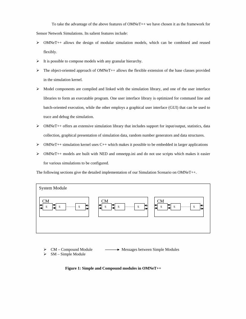
To take the advantage of the above features of OMNeT++ we have chosen it as the framework for
Sensor Network Simulations. Its salient features include:
OMNeT++ allows the design of modular simulation models, which can be combined and reused
flexibly.
It is possible to compose models with any granular hierarchy.
The object-oriented approach of OMNeT++ allows the flexible extension of the base classes provided
in the simulation kernel.
Model components are compiled and linked with the simulation library, and one of the user interface
libraries to form an executable program. One user interface library is optimized for command line and
batch-oriented execution, while the other employs a graphical user interface (GUI) that can be used to
trace and debug the simulation.
OMNeT++ offers an extensive simulation library that includes support for input/output, statistics, data
collection, graphical presentation of simulation data, random number generators and data structures.
OMNeT++ simulation kernel uses C++ which makes it possible to be embedded in larger applications
OMNeT++ models are built with NED and omnetpp.ini and do not use scripts which makes it easier
for various simulations to be configured.
The following sections give the detailed implementation of our Simulation Scenario on OMNeT++.
System Module
CM S S S
CM S S S
CM S S S
CM – Compound Module Messages between Simple Modules SM – Simple Module
Figure 1: Simple and Compound modules in OMNeT++
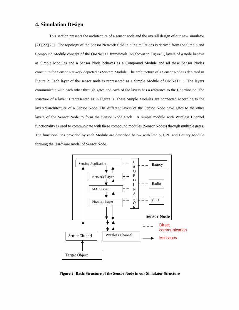
4. Simulation Design
This section presents the architecture of a sensor node and the overall design of our new simulator
[21][22][23]. The topology of the Sensor Network field in our simulations is derived from the Simple and
Compound Module concept of the OMNeT++ framework. As shown in Figure 1, layers of a node behave
as Simple Modules and a Sensor Node behaves as a Compound Module and all these Sensor Nodes
constitute the Sensor Network depicted as System Module. The architecture of a Sensor Node is depicted in
Figure 2. Each layer of the sensor node is represented as a Simple Module of OMNeT++. The layers
communicate with each other through gates and each of the layers has a reference to the Coordinator. The
structure of a layer is represented as in Figure 3. These Simple Modules are connected according to the
layered architecture of a Sensor Node. The different layers of the Sensor Node have gates to the other
layers of the Sensor Node to form the Sensor Node stack. A simple module with Wireless Channel
functionality is used to communicate with these compound modules (Sensor Nodes) through multiple gates.
The functionalities provided by each Module are described below with Radio, CPU and Battery Module
forming the Hardware model of Sensor Node.
Sensor Channel
Target Object
Sensing Application CoORDINATOR
Radio
Battery
CPU
Network Layer
MAC Layer
Physical Layer
Direct communication
MessagesWireless Channel
Sensor Node
Figure 2: Basic Structure of the Sensor Node in our Simulator Structure

A. CoOrdinator Module
CoOrdinator module has the functionalities that coordinate the activities of the hardware and the
software modules of the sensor node. It is basically used for inter layer Communication. The
CoOrdinator needs to be extended and functionality has to be added for access to properties of new
hardware or consumers added. As shown in the Figure 3, the CoOrdinator class has the reference to all
the layers in the sensor node and all the layers in the sensor node may access the CoOrdinator class
implementation. Thus through the CoOrdinator any layer may access and update the properties of the
other layer. For example the Battery Module needs to be informed on transmission or receiving the
packets by the Physical Module so that the energy consumption is updated at the node accordingly.
During simulation the CoOrdinator class is responsible for registering the Sensor Node to the Sensor
Network. Registering of the Sensor Node is an indication that the sensor node is up and functioning.
When the available energy is completely depleted, the node is unregistered from the sensor network.
To CoOrdinatorLayer ProtocolFrom CoOrdinator
From Upper Layer
To Upper Layer
From Bottom Layer
To BottomLayer
Figure 3: Representation of a Layer in Sensor Node
The connections between any two layers are done through gates and the communication is done
through messages. These are the various connections of any layer to the other layers and the CoOrdinator.
B. Hardware Model
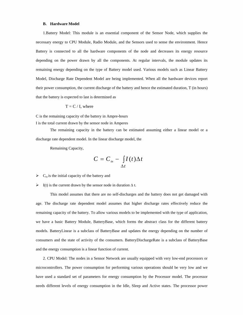
1.Battery Model: This module is an essential component of the Sensor Node, which supplies the
necessary energy to CPU Module, Radio Module, and the Sensors used to sense the environment. Hence
Battery is connected to all the hardware components of the node and decreases its energy resource
depending on the power drawn by all the components. At regular intervals, the module updates its
remaining energy depending on the type of Battery model used. Various models such as Linear Battery
Model, Discharge Rate Dependent Model are being implemented. When all the hardware devices report
their power consumption, the current discharge of the battery and hence the estimated duration, T (in hours)
that the battery is expected to last is determined as
T = C / I, where
C is the remaining capacity of the battery in Ampre-hours
I is the total current drawn by the sensor node in Amperes
The remaining capacity in the battery can be estimated assuming either a linear model or a
discharge rate dependent model. In the linear discharge model, the
Remaining Capacity,
∫∆
∆−=t
ttICC in )(
Cin is the initial capacity of the battery and
I(t) is the current drawn by the sensor node in duration ∆ t.
This model assumes that there are no self-discharges and the battery does not get damaged with
age. The discharge rate dependent model assumes that higher discharge rates effectively reduce the
remaining capacity of the battery. To allow various models to be implemented with the type of application,
we have a basic Battery Module, BatteryBase, which forms the abstract class for the different battery
models. BatteryLinear is a subclass of BatteryBase and updates the energy depending on the number of
consumers and the state of activity of the consumers. BatteryDischargeRate is a subclass of BatteryBase
and the energy consumption is a linear function of current.
2. CPU Model: The nodes in a Sensor Network are usually equipped with very low-end processors or
microcontrollers. The power consumption for performing various operations should be very low and we
have used a standard set of parameters for energy consumption by the Processor model. The processor
needs different levels of energy consumption in the Idle, Sleep and Active states. The processor power

consumption model is very important and ignoring that will lead to incorrect trends in power consumption
in the network. New processor models with enhanced features and improved energy consumption levels
can be incorporated in this module for testing various kinds of applications. CPUBase abstract class forms
the basis for different CPU models and it defines the interfaces of this module with CoOrdinator and the
Battery. CPUSimple has implementation of the power consumption of the CPU in different states: Idle,
Sleep and Active.
3. Radio Model: This model is used to characterize the antenna property of a node. RadioBase is an
abstract class for the different Radio models. RadioSimple, a subclass of RadioBase updates the energy of
the battery depending on the state of the Radio: idle, sleep, transmit, and receive. The values for the
different properties of the hardware and consumers maybe provided through the configuration file.
C. Wireless Channel Model:
The Wireless Channel Module controls and maintains all potential connections between the Sensor
Nodes. These static connections are provided from all the nodes to the Wireless Channel Module and from
the module to all the nodes in the NED file. These connections enable Sensor Nodes to exchange data and
communicate with each other. Any message from a node is sent to all the neighbors within its transmission
region with a delay d where d is (Distance between the communicating Sensor Nodes) / Speed of Light.
Various Radio Propagation models are used to predict the received signal power of each packet.
These models affect the communicating region between any 2 nodes and are derived by the Wireless
Channel.
1. Free Space Propagation Model: The free space propagation model assumes the ideal
propagation condition that there is only one clear line-of-sight path between the transmitter and receiver. H.
T. The received signal power in free space at distance _ from the transmitter is estimated as: [25]
2222rttr L*d*)4/()*G*G*P(P πλ=
Pt is the transmitted signal power
Pr is the received signal power
G t, G r are the antenna gains of the transmitter and the receiver respectively.
L is the system loss, and _ is the wavelength.
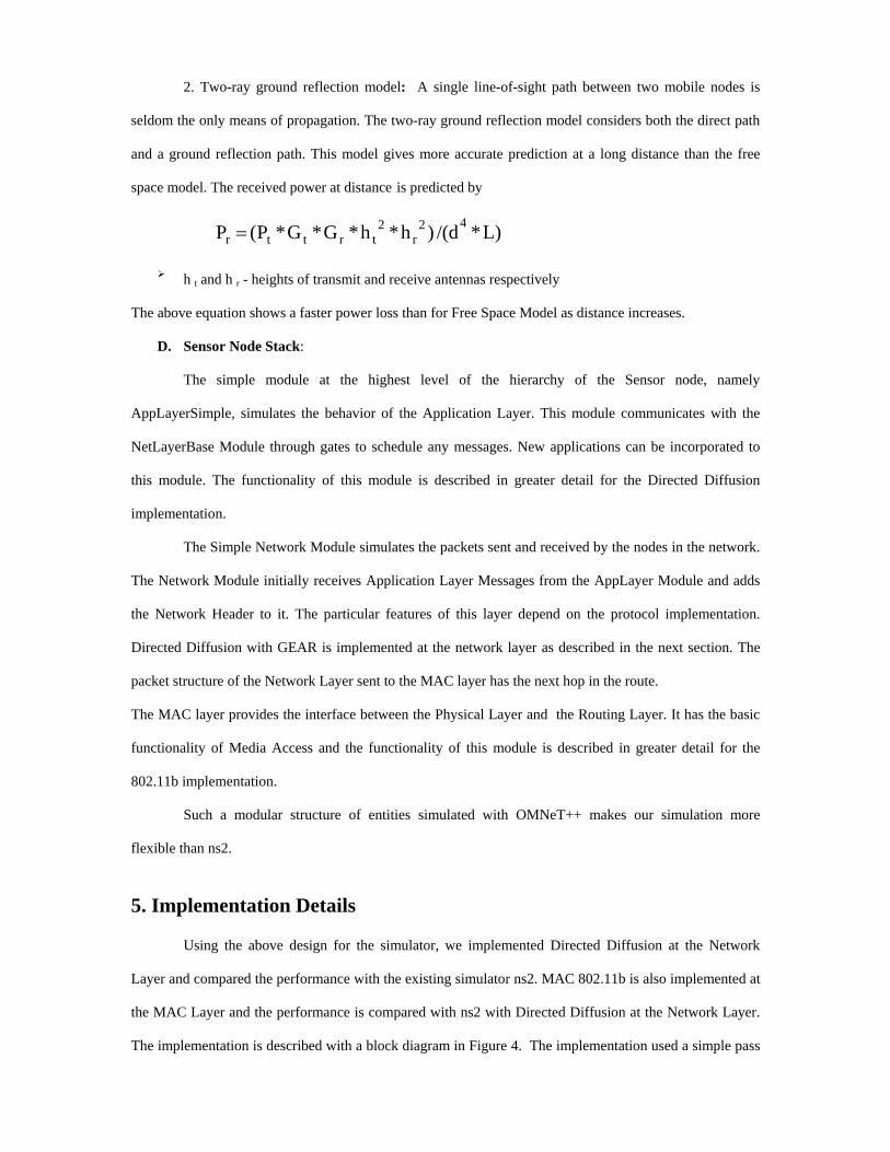
2. Two-ray ground reflection model: A single line-of-sight path between two mobile nodes is
seldom the only means of propagation. The two-ray ground reflection model considers both the direct path
and a ground reflection path. This model gives more accurate prediction at a long distance than the free
space model. The received power at distance _ is predicted by
)L*d/()h*h*G*G*P(P 42r
2trttr =
h t and h r - heights of transmit and receive antennas respectively
The above equation shows a faster power loss than for Free Space Model as distance increases.
D. Sensor Node Stack:
The simple module at the highest level of the hierarchy of the Sensor node, namely
AppLayerSimple, simulates the behavior of the Application Layer. This module communicates with the
NetLayerBase Module through gates to schedule any messages. New applications can be incorporated to
this module. The functionality of this module is described in greater detail for the Directed Diffusion
implementation.
The Simple Network Module simulates the packets sent and received by the nodes in the network.
The Network Module initially receives Application Layer Messages from the AppLayer Module and adds
the Network Header to it. The particular features of this layer depend on the protocol implementation.
Directed Diffusion with GEAR is implemented at the network layer as described in the next section. The
packet structure of the Network Layer sent to the MAC layer has the next hop in the route.
The MAC layer provides the interface between the Physical Layer and the Routing Layer. It has the basic
functionality of Media Access and the functionality of this module is described in greater detail for the
802.11b implementation.
Such a modular structure of entities simulated with OMNeT++ makes our simulation more
flexible than ns2.
5. Implementation Details Using the above design for the simulator, we implemented Directed Diffusion at the Network
Layer and compared the performance with the existing simulator ns2. MAC 802.11b is also implemented at
the MAC Layer and the performance is compared with ns2 with Directed Diffusion at the Network Layer.
The implementation is described with a block diagram in Figure 4. The implementation used a simple pass

through Physical Layer, a simple WirelessChannel Module with the Application Layer generating query
packets and forwarding to Network Layer.
Query Generator
Directed Diffusion
802_11_MACMACLayerBase
COORDINATOR
MODULE
QueueNetLayerBase
MAC Packet
AppLayerBase
Ntw_Pkt Decapsulator
Encapsulator
PhysicalSimple Module
Battery Module
CPU Module
Radio Module
Wireless ChannelModule
Free Space Propagation
Tworay Propogation
Node Tracking Module
Figure 4: Implementation Scenario
Query path from Network Layer to MAC
Query path from MAC to Network Layer

A. Directed Diffusion with GEAR
We have implemented Directed Diffusion[7] along with Geographic Routing. The Application Layer
generates interests that specify the region, the kind of data required and rate of delivery of data. Nodes that
initiate the interest are called subscribers. On receiving the interest message, the network layer
Query - attribute Query - rate of data Query - duration
Figure 5: Structure of a query
broadcasts beacon messages in the network. The immediate neighbors of the node on receiving beacon
messages reply back with beacon-reply type of message that contains their geographic location and the
energy left in them. On receiving the beacon-reply messages, the neighbor table of the node that sent the
beacon is updated. The node waits a fixed duration of time to receive the beacon-reply from all the
neighbors. The interest message is then forwarded to the node that has a lower estimated cost to the region
as calculated by the GEAR protocol[17]. The next node follows the same procedure and forwards the
message towards the region by Geographic Routing. If a node in the path does not have any neighbors or
all its neighbors are away from the region, then it sends a message to its parent node that it is a dead-end.
The parent node on updating the cost of the unreachable node, forwards the query in an alternate route
towards the region. In the target region, the interest is dessiminated by using recursive flooding. The
interest cache is maintained at each of the nodes in the path with its gradient of interest to each of the
neighbors. The nodes in the region that have the specified properties of the interest send out data. Nodes
that send data out are referred to as Publishers.
The data is marked as Exploratory to reinforce the path that was taken by the interest. On
receiving the data marked as Exploratory by the subscriber, a positive reinforcement message is sent out by
the Subscriber node. Each node on the path forwards this message - thus reinforcing the path to the region.
When a node reinforces a path, its cost to the region is known and this cost is sent back to its source node,
which updates the cost information of that node to the particular region of interest. Thus the path with the
lowest cost is always maintained, reinforcing the route.

The data from the region follows the path established by the reinforced messages. The nodes in the
region send out data at the rate that is specified in the query. Data caching is implemented in intermediate
nodes and so the data requested by different subscribers from the same region can be satisfied by the
common node in the path thus reducing the traffic and redundant messages. The data marked as exploratory
are sent to identify better paths and reinforce at regular intervals. Also the neighbor- updating procedure is
carried out, i.e. at regular intervals the beacon messages are broadcast and beacon-reply messages are sent
by neighbors thus maintaining latest neighbor information.
C. 802.11 MAC
The MAC layer places the network packet on the Wireless Channel. The NetworkPacket maybe a
broadcast or unicast packet to a specific node (sink node). Any network layer packet received by the MAC-
802-11 [3][15][26] module is encapsulated into MAC frame with the MAC header added to it.
The Network layer packets have the information whether the packet has to be broadcast or unicast.
Broadcast packet is encapsulated into Broadcast MAC frame with appropriate MAC Header and is put in
the Messages-queue of the MAC Layer. If the Network packet is for a particular destination, RTS frame is
created and is inserted in the Messages-queue of MAC layer. If the Network packet length is more than the
MAC frame, it is fragmented and the fragments for that Network Packet are created with MAC headers and
are inserted into the Fragments Queue.
The MAC layer then waits for the channel to be idle to send its frame from the Messages-queue.
MAC layer has a NAV Timer, which specifies the busy/idle state of the medium. NAV Timer set for a node
implies that the channel is busy. When the NAV Timer expires the MAC layer waits for the channel to be
free for DIFS time and if the channel is still idle after DIFS timer gets expired, it then goes into Exponential
BackOff. It then waits for a random time set by the BackOff Timer. The BackOff Timer decrements its
value during the idle period of channel. The node whose BackOff Timer expires earlier will get the chance
to transmit its next frame. All the intermediate nodes receive this frame, set their NAVTimer to the value
obtained from the Header field of the received frame. Then the BackOff Timer of the intermediate nodes is
stopped from decrementing. Once the channel becomes idle (when the NAVTimer expires) all the nodes
start decrementing their BackOff Timer. The node whose Back Off Timer expired earlier and got the
channel will send the first message from the Messages Queue. If it is a broadcast message, then all the
nodes in its region receive it and the MAC layer of those nodes decapsulate the Network packet and send it
to the Network Layer. If it is a RTS frame, the Destination node checks whether its NAV timer is set or not
(its transmission region is busy or not) and then responds to it by sending CTS. All the other intermediate
nodes receiving this RTS update their NAV Timer to the CTS+DATA+ACK duration which implies that
the channel is busy for that duration and hence refrain from transmitting during this interval. If the
Destination node receives more than two RTS requests within a time interval then collision occurs and the
Destination node does not respond (send CTS) to any of these RTS requests. The Source node which is
sending RTS have an RTSExpired Timer set for RTS frames, when they are sent to the Destination node.
This timer is scheduled to expire after RTS+CTS duration. If the Source node does not receive CTS within
this duration, RTSExpired Timer gets expired and retry counter of that RTS frame is incremented. If the
retry counter is less than ShortRetyLimit (as per the specification), then the Contention Window is doubled
and the random time set by the BackOff Timer is chosen between 1 and the Contention Window size. If the
retry counter reaches ShortRetryLimit, then the message (RTS and corresponding Fragment) is dropped by
the MAC.
If the Destination node responds to RTS by sending back the CTS, the intermediate nodes for CTS
will update their NAVTimer obtained from the Header field of CTS frame (Data+Ack duration) and hence
refrain from transmitting during this interval. Once the Source node gets the CTS, it will send the
corresponding fragment of the Network Packet to the Destination and waits for an Acknowledgement. The
Destination node upon receiving the Data frame extracts the Network packet, sends it to the Network layer
and sends back the Acknowledgement to the Source node. Once the Source node gets the
Acknowledgement it checks and sends if there are any other fragments to be sent to this node without any
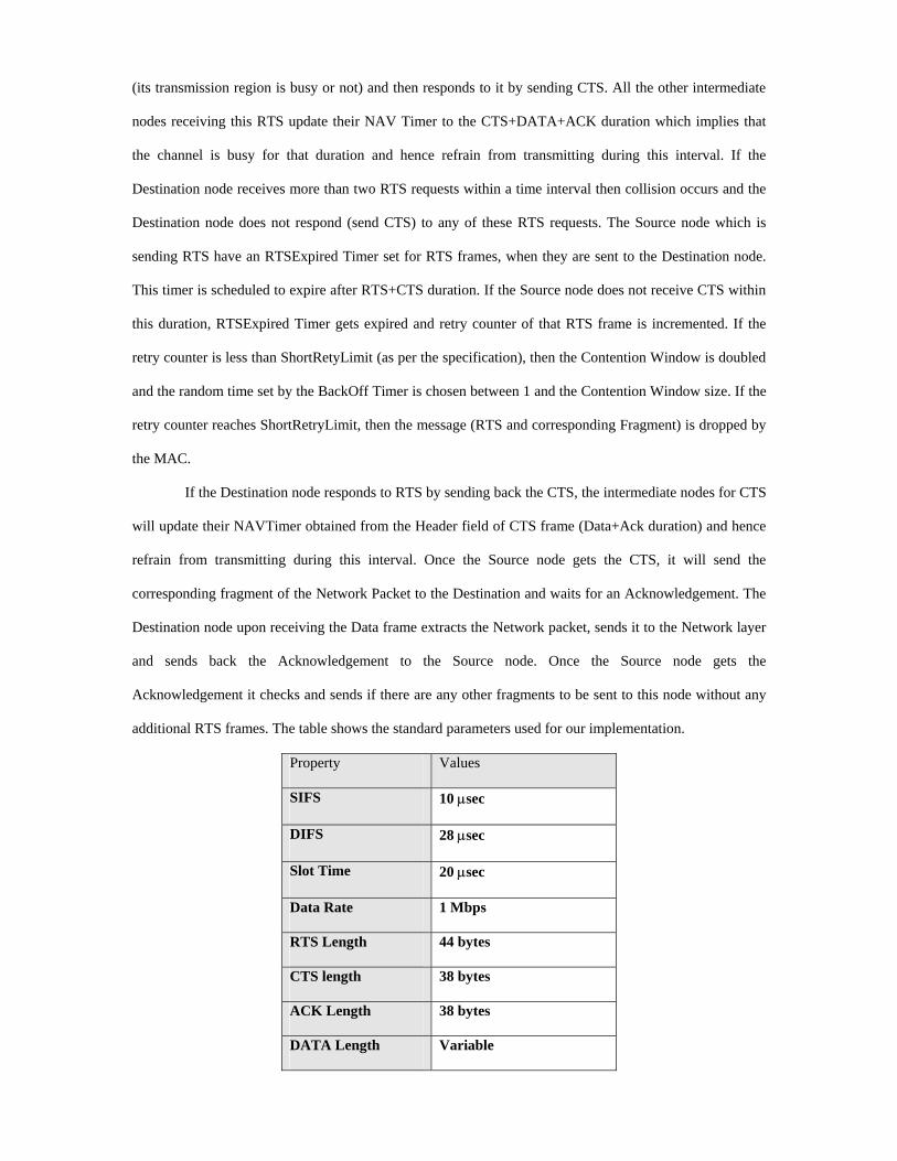
additional RTS frames. The table shows the standard parameters used for our implementation.
Property Values
SIFS 10 µsec
DIFS 28 µsec
Slot Time 20 µsec
Data Rate 1 Mbps
RTS Length 44 bytes
CTS length 38 bytes
ACK Length 38 bytes
DATA Length Variable
6. Experimental Results:
In this section, we present results from three different studies. First, we establish that the
DirectedDiffusion simulation in our work is consistent with the Diffusion implementation in ns2. Next, we
compare the performance, with respect to execution time and memory used, between our simulation and
that of ns2.
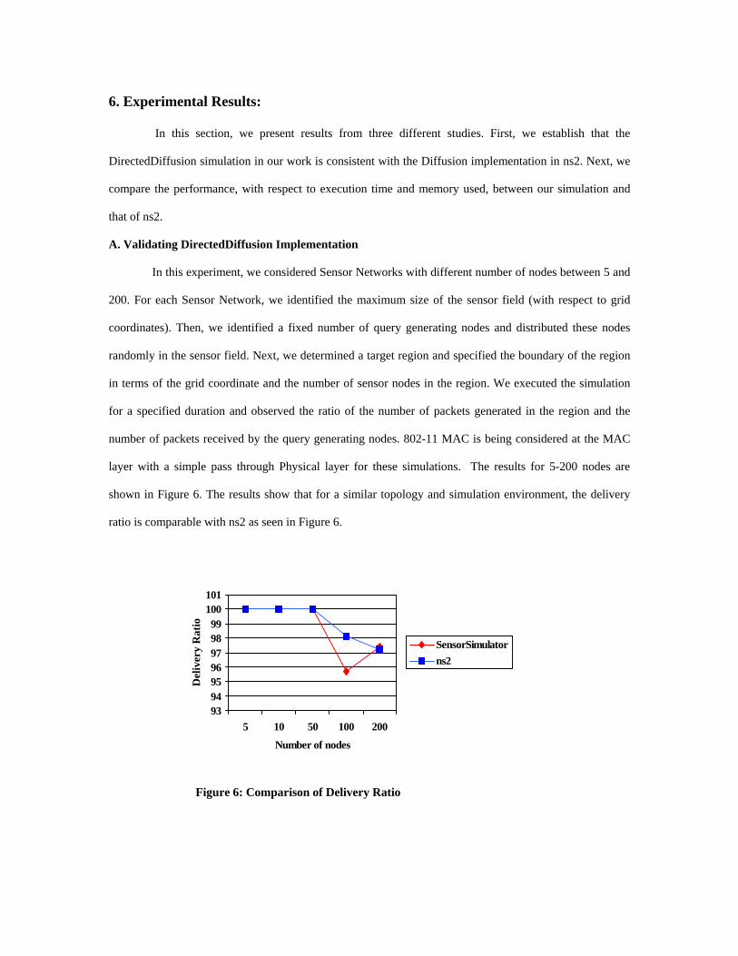
A. Validating DirectedDiffusion Implementation
In this experiment, we considered Sensor Networks with different number of nodes between 5 and
200. For each Sensor Network, we identified the maximum size of the sensor field (with respect to grid
coordinates). Then, we identified a fixed number of query generating nodes and distributed these nodes
randomly in the sensor field. Next, we determined a target region and specified the boundary of the region
in terms of the grid coordinate and the number of sensor nodes in the region. We executed the simulation
for a specified duration and observed the ratio of the number of packets generated in the region and the
number of packets received by the query generating nodes. 802-11 MAC is being considered at the MAC
layer with a simple pass through Physical layer for these simulations. The results for 5-200 nodes are
shown in Figure 6. The results show that for a similar topology and simulation environment, the delivery
ratio is comparable with ns2 as seen in Figure 6.
93949596979899
100101
5 10 50 100 200
Number of nodes
Del
iver
y R
atio
SensorSimulatorns2
Figure 6: Comparison of Delivery Ratio
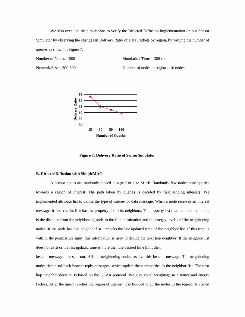
We also executed the simulations to verify the Directed Diffusion implementation on our Sensor
Simulator by observing the changes in Delivery Ratio of Data Packets by region, by varying the number of
queries as shown in Figure 7.
Number of Nodes = 500 Simulation Time = 300 sec
Network Size = 500-500 Number of nodes in region = 10 nodes
76
7880
8284
86
15 30 50 100
Number of Queries
Del
iver
y R
atio
Figure 7: Delivery Ratio of SensorSimulator
B. DirectedDiffusion with SimpleMAC:
N sensor nodes are randomly placed in a grid of size M ×P. Randomly few nodes send queries
towards a region of interest. The path taken by queries is decided by first sending interests. We
implemented attribute list to define the type of interest or data message. When a node receives an interest
message, it first checks if it has the property list of its neighbors. The property list that the node maintains
is the distance from the neighboring node to the final destination and the energy level’s of the neighboring
nodes. If the node has this neighbor list it checks the last updated time of the neighbor list. If this time is
with in the permissible limit, this information is used to decide the next hop neighbor. If the neighbor list
does not exist or the last updated time is more than the desired time limit then
beacon messages are sent out. All the neighboring nodes receive this beacon message. The neighboring
nodes then send back beacon reply messages, which update these properties in the neighbor list. The next
hop neighbor decision is based on the GEAR protocol. We give equal weightage to distance and energy
factors. After the query reaches the region of interest, it is flooded to all the nodes in the region. A visited

node list is maintained to avoid going into a loop. When a node in the region of interest receives an interest
it sends back an exploratory message to the source of the interest. The exploratory message follows the
reverse path taken by the interest message. It gets the reverse path information from the nodes. When this
exploratory message reaches the source node, the source node reinforces the path by sending back
reinforcements. The reinforcements might or might not follow the same path as the initial interest message.
On the arrival of the reinforcements the nodes in the region of interest start sending back data messages at
the rate specified in the interest. At regular intervals these data messages are marked as exploratory. When
the source receives a data message marked as exploratory it sends reinforcements to rebuild the path. This
would repair any holes that might have formed in the path
In order to test the performance of the simulation we ran the setup with queries generated by 10
nodes at random locations in the network. A similar test was performed with 100 nodes generating queries.
The queries follow a multi-hop route to the region following the procedure mentioned above. Once the
query reaches the region the data is sent back once every 5 seconds for the complete simulation time by all
the nodes in the region. The objective of this kind of setup is to check whether the simulation framework is
able to handle the traffic generated and run to completion as well as to check the amount of time required to
run the simulation. Figures 8 and 9 shows the performance of the two simulators (ns2 Vs. our Simulation)
for the setup with 10 nodes and 100 nodes generating queries. For these experiments a pass through Simple
MAC and a simple Physical Layer are being considered. It is can be observed that
the performance of both the simulators ns2 and SensorSimulator showed similar results at less number of
nodes in the network. As the number of nodes in the network increases, SensorSimulator is able to handle
the traffic and the events generated in a better fashion so as to complete the simulation in a reasonable time
faster than ns2. It has been observed that ns2 ran out of memory for network above 2000 nodes. It can be
also observed in the figures that the execution time for the simulation run on the SensorSimulator is less
than that for ns2 for the same simulation results obtained on both the simulators. During the simulation
runs, we measured the memory allocated before the start of the simulation, i.e it gives the memory usage
for the initialization and the setup of the objects of the simulation. The memory usage during the simulation
was also measured. The results for the memory usage are as shown in Figure 10 and Figure 11 when 10
nodes are sending queries and Figure 12 and Figure 13 show the performance of the simulators for 100
nodes sending queries to the region. This shows that the data structures used for the simulation are used in a
scalable manner to represent the different classes and the interaction with the framework. It can also be
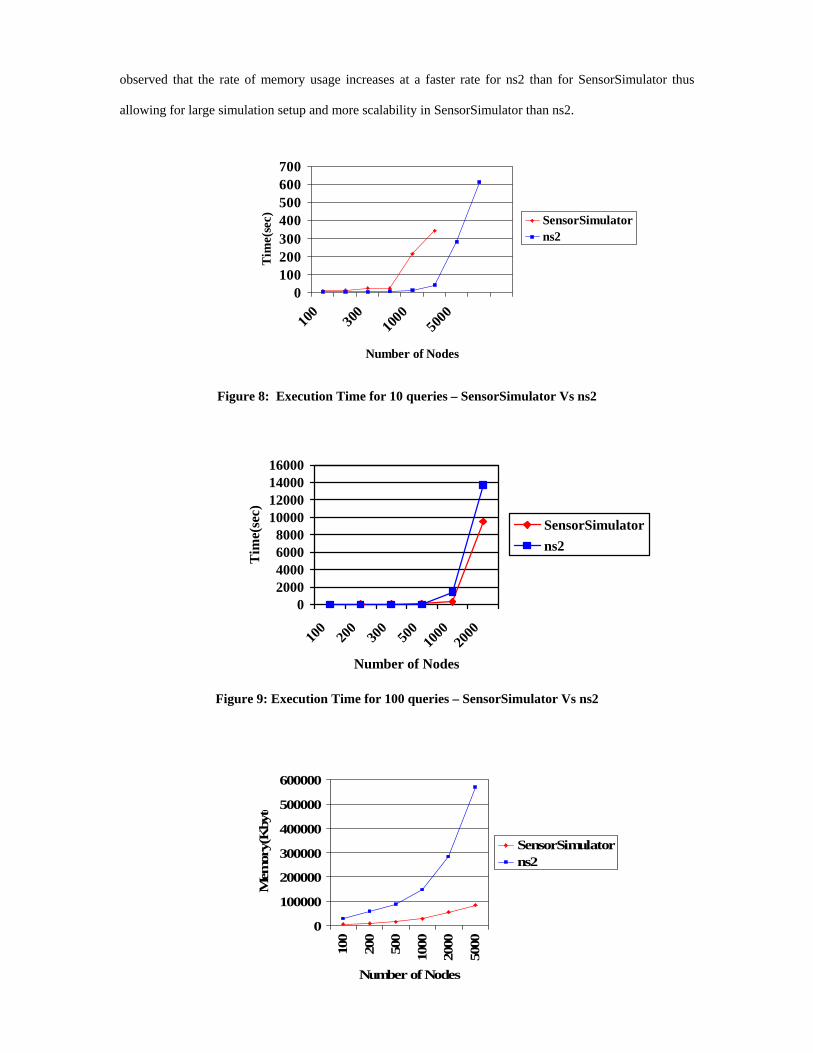
observed that the rate of memory usage increases at a faster rate for ns2 than for SensorSimulator thus
allowing for large simulation setup and more scalability in SensorSimulator than ns2.
0100200300400500600700
100
300
1000
5000
Number of Nodes
Tim
e(se
c) SensorSimulatorns2
Figure 8: Execution Time for 10 queries – SensorSimulator Vs ns2
02000400060008000
10000120001400016000
100
200
300
500
1000
2000
Number of Nodes
Tim
e(se
c)
SensorSimulatorns2
Figure 9: Execution Time for 100 queries – SensorSimulator Vs ns2
0
100000
200000
300000
400000
500000
600000
100
200
500
1000
2000
5000
Number of Nodes
Mem
ory(
Kby
te
SensorSimulatorns2
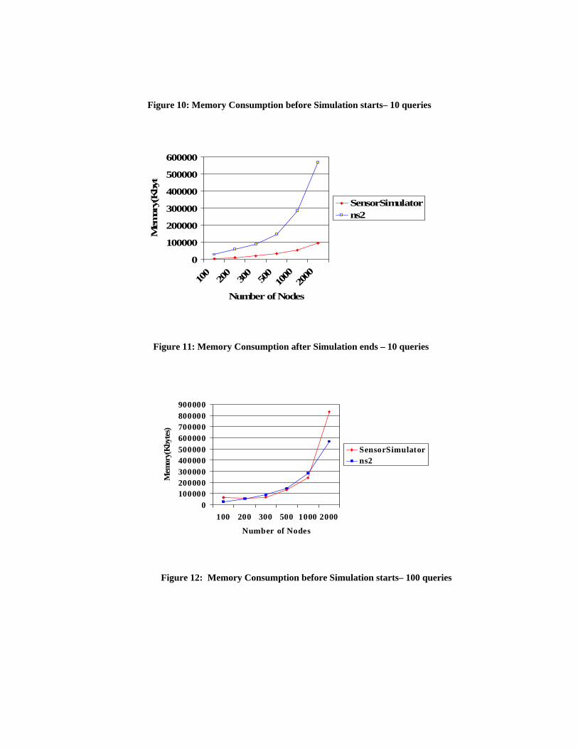
Figure 10: Memory Consumption before Simulation starts– 10 queries
0
100000
200000
300000
400000
500000
600000
100
200
300
500
1000
2000
Number of Nodes
Mem
ory(
Kby
te
SensorSimulatorns2
Figure 11: Memory Consumption after Simulation ends – 10 queries
0100000200000300000400000500000600000700000800000900000
100 200 300 500 1000 2000
Number of Nodes
Mem
ory(
Kbyt
es)
SensorSimulatorns2
Figure 12: Memory Consumption before Simulation starts– 100 queries

0
100000
200000
300000
400000
500000
600000
100
200
300
500
1000
2000
Number of Nodes
Mem
ory(
Kby
te
SensorSimulatorns2
Figure 13: Memory Consumption after Simulation ends – 100 queries
C. DirectedDiffusion with IEEE 802.11 MAC
This series of experiments use MAC 802.11b at the MAC Layer and compare the performance of
SensorSimulator with ns2. A simple pass through Physical Layer is considered. The simulation is run for
100, 500, 1000 and 2000 nodes. The nodes in the Sensor Network are deployed randomly in various
locations with the network size being configurable in the omnetpp.ini file. Figure 14 shows the relative
performance. The set up for them is:
Number of Queries: 10 Network Dimension – Varies with the number of nodes
Number of Nodes in Region: 10 Simulation Time = 300 sec
0
500
1000
1500
2000
2500
3000
100 500 1000 2000Number of Nodes
Tim
e(se
c
SensorSimulatorns2
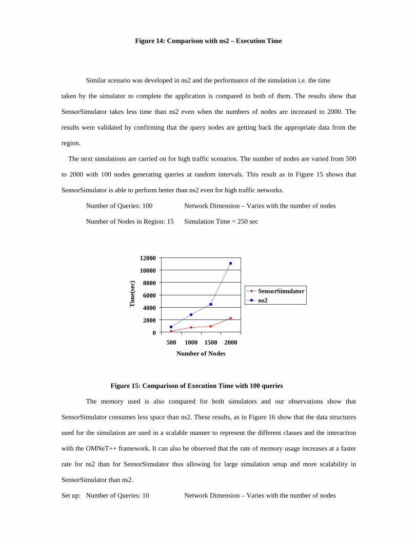
Figure 14: Comparison with ns2 – Execution Time
Similar scenario was developed in ns2 and the performance of the simulation i.e. the time
taken by the simulator to complete the application is compared in both of them. The results show that
SensorSimulator takes less time than ns2 even when the numbers of nodes are increased to 2000. The
results were validated by confirming that the query nodes are getting back the appropriate data from the
region.
The next simulations are carried on for high traffic scenarios. The number of nodes are varied from 500
to 2000 with 100 nodes generating queries at random intervals. This result as in Figure 15 shows that
SensorSimulator is able to perform better than ns2 even for high traffic networks.
Number of Queries: 100 Network Dimension – Varies with the number of nodes
Number of Nodes in Region: 15 Simulation Time = 250 sec
0
2000
4000
6000
8000
10000
12000
500 1000 1500 2000
Number of Nodes
Tim
e(se
c)
SensorSimulatorns2
Figure 15: Comparison of Execution Time with 100 queries
The memory used is also compared for both simulators and our observations show that
SensorSimulator consumes less space than ns2. These results, as in Figure 16 show that the data structures
used for the simulation are used in a scalable manner to represent the different classes and the interaction
with the OMNeT++ framework. It can also be observed that the rate of memory usage increases at a faster
rate for ns2 than for SensorSimulator thus allowing for large simulation setup and more scalability in
SensorSimulator than ns2.
Set up: Number of Queries: 10 Network Dimension – Varies with the number of nodes

Number of nodes in region: 5 Simulation Time = 300 sec
0
100000
200000
300000
400000
500000
600000
700000
100 500 1000 2000
Number of Nodes
Mem
ory(
Kbyt
es)
SensorSimulatorns2
Figure 16: Comparison of Memory Consumption
7. Conclusions and Future Work
The results presented in this paper show that OMNeT++ is a viable discrete event simulation
framework for studying both the networking aspects and the distributed computing aspects of sensor
networks. We presented the architecture of a sensor node that is used in the simulator and the general
architecture of the simulator.
Based on our studies with the IEEE 802.11 MAC and Directed Diffusion integrated with GEAR,
we conclude that our simulator is at least an order of magnitude faster than ns2 and uses memory more
efficiently than ns2. The modular structure of compound modules and the ease of configuring simulation
scenarios via an initialization file offers us a tremendous amount of flexibility to model and study the
dynamic behaviors of both the sensor network and the application environment such networks are expected
to operate.
8. Acknowledgements: The authors acknowledge the assistance of students and faculty in the Sensor Network Group for
their contributions towards the development of SensorSimulator. The authors also acknowledge the CCT
for providing infrastructure facilities for the development of Sensor Network Laboratory.
References
[1] J. Agre, L. Clare, and S. Sastry. A Taxonomy for Distributed Real-time Control Systems. Advances in Computers, Ed. M. Zelkowitz, 49:303–352, 1999. [2] I.F. Akyildiz, W. Su, Y. Sankarasubramaniam, and E. Cayirci. Wireless Sensor Networks: A Survey. Computer Networks, 38:393–422, 2002. [3] V. Bharghavan, A. Demers, S. Shenker, and L. Zhang. MACAW: A Media Access Protocol for Wireless LAN’s. In ACM SIGCOMM 1994, 1994. [4] K. Fall and K. Varadhan. NS-2 Network Simulator. University of California, Berkeley, 2004.
[5] G.S. Fishman. Principles of Discrete Event Simulation. Wiley, 1978.
[6] J. Hill, R. Szewczyk, A. Woo, S. Hollar, D. Culler, and K. Pister. System Architecture Directions for Networked Sensors. In ACM Sigplan Notices, volume 35, pages 93–104, 2000. [7] C. Intanagonwiwat, R. Govindan, D. Estrin, J. Heidemann, and F. Silva. Directed Diffusion for Wireless Sensor Networking. IEEE/ACM Transactions on Networking, 11(1):2–16, February 2003. [8] D.B. Johnson. The Rice University Monarch Project. Technical Report, Rice University, 2004.
[9] J. Misra. Distributed discrete-event simulation. ACM Computing Surveys, Vol. 18, No. 1, pp. 39-65, March 1986. [10] OPNET Technolgies, Inc. OPNET Modeler.
[11] S. Park, A. Savvides, and M.B. Srivastava. SensorSim: a simulation framework for sensor networks. In Proceedings of the 3rd ACM International DRAFT workshop on Modeling, analysis and simulation of wireless and mobile systems, pages 104–111, 2000. [12] S. Sastry and S.S. Iyengar. Real-time Sensor-Actuator Networks. International Journal of Distributed Sensor Networks, [13] S. Sastry and S.S. Iyengar. Sensor Technologies for Future Automation Systems. Sensor Letters, 2(1): 9–17, 2004. [14] A. Sobieh and J.C. Hou. A simulation framework for sensor networks in J-sim. Technical Report UIUCDCS-R-2003-2386, University of Illinois at Urbana-Champaign, Department of Computer Science, November 2003. [15] A. Tannenbaum. Computer Networks. Prentice Hall, 2002.
[16] A. Vargas. OMNET++Discrete Event Simulation System, version 2.3 edition, 2003.
[17] Y. Yu, R. Govindan, and D. Estrin. Geographial and energy aware routing: A recursive data dissemination protocol for wireless sensor networks, August 2001. [18] X. Zeng, R. Bagrodia, and M. Gerla. Glomosim: A library for parallel simulation of large-scale wireless networks. In Workshop on Parallel and Distributed Simulation, pages 154–161, 1998. [19] S. S. Iyengar and R. R. Brooks, “Distributed Sensor Networks” CRC press ‘Inc. Dec 28, 2004 pp 1188
[20] http://www.cs.rpi.edu/~cheng3/sense/
[21] LSU SensorSimulator (LSU SenSim-Version1, January 2005) User Manual. Authors: LSU Research
Group, Dept. Of Computer Science, Louisiana State University, Baton Rouge, Louisiana – 70803.
[22] “SenSim: A Wireless Sensor Network Simulation Template” Project by Shivakumar Basavaraju, Department Of Computer Science, Louisiana State University, Baton Rouge, LA – 70808. [23] “SensorSimulator: A Simulation Framework for SensorNetworks” Thesis by Cariappa Mallanda, Department of Computer Science, Louisiana State University, Baton Rouge, LA – 70808. [24] S. Sastry, SmartSpace for Automation, Assembly Automation, Vol. 24, No. 2, 2004, pages 201-209.
[25] http://www.isi.edu/nsnam/ns/ns-documentation.html
[26] “Information technology - telecommunication and information exchange between systems - local and metropolitan area networks – specific requirements - part 11: Wireless lan medium access control (mac) and physical layer (phy) specifications,” IEEE Standard, Tech. Rep., 1999