
Simulating the value of Options - University of...
46
Chapter 5 Simulating the value of Options Asian Options An Asian option, at expiration T, has value determined not by the closing price of the underlying asset as for a European option, but on an average price of the asset over an interval. For example a discretely sampled Asian call op- tion on an asset with price process S(t) pays an amount on maturity equal to max(0, ¯ S k − K) where ¯ S k = 1 k P k i=1 S(iT /k) is the average asset price at k equally spaced time points in the time interval (0,T ). Here, k depends on the frequency of sampling (e.g. if T = .25 (years) and sampling is weekly, then k = 13. If S(t) follows a geometric Brownian motion, then ¯ S k is the sum of lognormally distributed random variables and the distribution of the sum or av- erage of lognormal random variables is very difficult to express analytically. For this reason we will resort to pricing the Asian option using simulation. Notice, however that in contrast to the arithmetic average, the distribution of the geo- metric average has a distribution which can easily be obtained. The geometric 265
-
Upload
phamkhuong -
Category
Documents
-
view
216 -
download
3
Transcript of Simulating the value of Options - University of...

Chapter 5
Simulating the value of
Options
Asian Options
An Asian option, at expiration T, has value determined not by the closing price
of the underlying asset as for a European option, but on an average price of
the asset over an interval. For example a discretely sampled Asian call op-
tion on an asset with price process S(t) pays an amount on maturity equal
to max(0, Sk −K) where Sk = 1k
Pki=1 S(iT/k) is the average asset price at k
equally spaced time points in the time interval (0, T ). Here, k depends on the
frequency of sampling (e.g. if T = .25 (years) and sampling is weekly, then
k = 13. If S(t) follows a geometric Brownian motion, then Sk is the sum of
lognormally distributed random variables and the distribution of the sum or av-
erage of lognormal random variables is very difficult to express analytically. For
this reason we will resort to pricing the Asian option using simulation. Notice,
however that in contrast to the arithmetic average, the distribution of the geo-
metric average has a distribution which can easily be obtained. The geometric
265

266 CHAPTER 5. SIMULATING THE VALUE OF OPTIONS
mean of n valuesX1, ...,Xn is (X1X2...Xn)1/n = exp{ 1nPni=1 ln(Xi)} and if the
random variables Xn were each lognormally distributed then this results adding
the normally distributed random variables ln(Xi) in the exponent, a much more
familiar operation. In fact the sum in the exponent 1n
Pni=1 ln(Xi) is normally
distributed so the geometric average will have a lognormal distribution.
Our objective is to determine the value of the Asian option E(V1) with
V1 = e−rTmax(0, Sk −K)
Since we expect geometric means to be close to arithmetic means, a reasonable
control variate is the random variable V2 = e−rTmax(0, Sk − K) where Sk =
{Qki=1 S(iT/k)}
1/k is the geometric mean. Assume that V1 and V2 obtain from
the same simulation and are therefore possibly correlated. Of course V2 is only
useful as a control variate if its expected value can be determined analytically
or numerically more easily than V1 but in view of the fact that V2 has a known
lognormal distribution, the prospects of this are excellent. Since S(t) = S0eY (t)
where Y (t) is a Brownian motion with Y (0) = 0, drift r− σ2/2 and diffusion σ,
it follows that Sk has the same distribution as does
S0 exp{1
k
kXi=1
Y (iT/k)}. (5.1)
This is a weighted average of the independent normal increments of the process
and therefore normally distributed. In particular if we set
Y =1
k
kXi=1
Y (iT/k)
=1
k[k(Y (T/k)) + (k − 1){Y (2T/k)− Y (T/k)}+ (k − 2){Y (3T/k)− Y (2T/k)}
+ ...+ {Y (T )− Y ((k − 1)T/k)}],
ASIAN OPTIONS 267
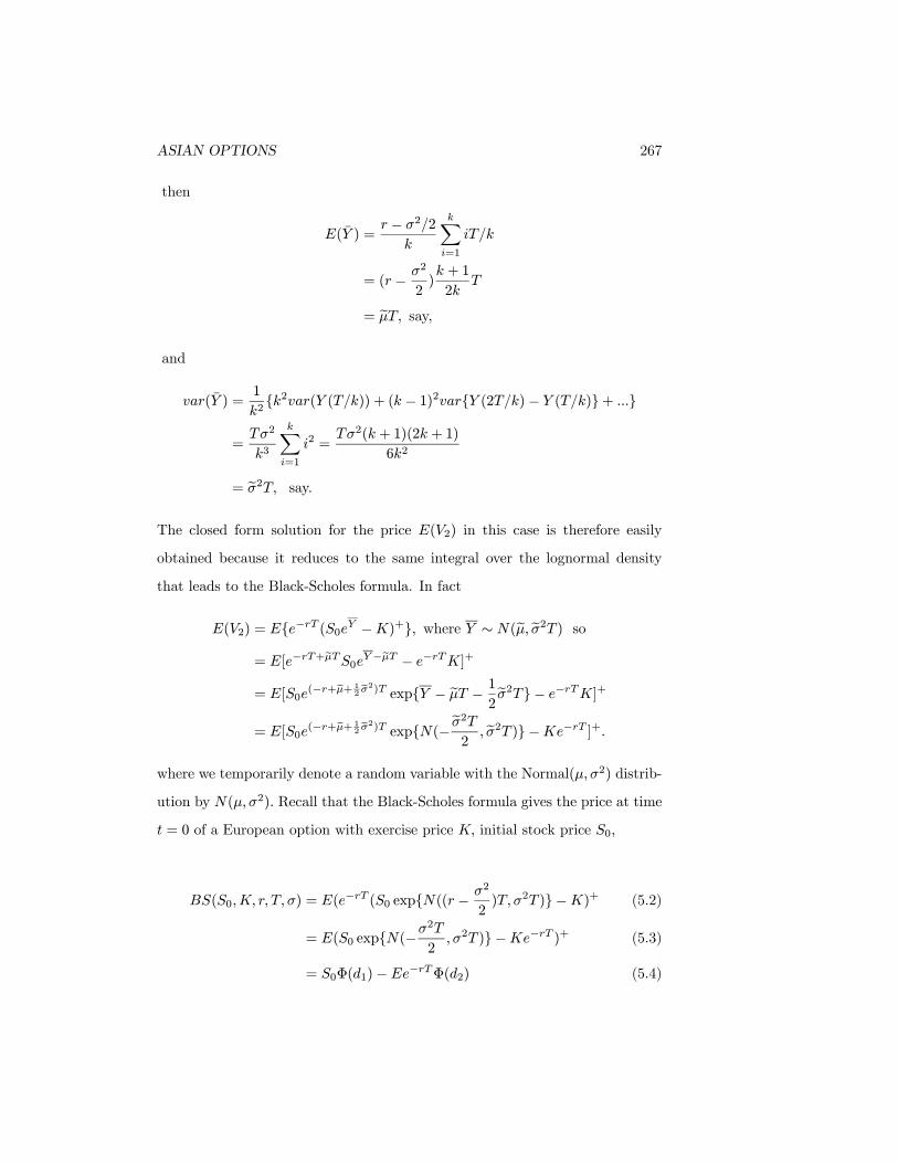
then
E(Y ) =r − σ2/2
k
kXi=1
iT/k
= (r −σ2
2)k + 1
2kT
= eµT, say,and
var(Y ) =1
k2{k2var(Y (T/k)) + (k − 1)2var{Y (2T/k)− Y (T/k)}+ ...}
=Tσ2
k3
kXi=1
i2 =Tσ2(k + 1)(2k + 1)
6k2
= eσ2T, say.The closed form solution for the price E(V2) in this case is therefore easily
obtained because it reduces to the same integral over the lognormal density
that leads to the Black-Scholes formula. In fact
E(V2) = E{e−rT (S0eY −K)+}, where Y ∼ N(eµ, eσ2T ) so
= E[e−rT+eµTS0eY−eµT − e−rTK]+= E[S0e
(−r+eµ+ 12eσ2)T exp{Y − eµT − 1
2eσ2T}− e−rTK]+
= E[S0e(−r+eµ+ 1
2eσ2)T exp{N(−eσ2T2, eσ2T )}−Ke−rT ]+.
where we temporarily denote a random variable with the Normal(µ,σ2) distrib-
ution by N(µ,σ2). Recall that the Black-Scholes formula gives the price at time
t = 0 of a European option with exercise price K, initial stock price S0,
BS(S0,K, r, T,σ) = E(e−rT (S0 exp{N((r −
σ2
2)T,σ2T )}−K)+ (5.2)
= E(S0 exp{N(−σ2T
2,σ2T )}−Ke−rT )+ (5.3)
= S0Φ(d1)− Ee−rTΦ(d2) (5.4)

268 CHAPTER 5. SIMULATING THE VALUE OF OPTIONS
where
d1 =log(S0/K) + (r + σ2/2)T
σ√T
, d2 = d1 − σ√T .
Thus E(V2) is given by the Black-Scholes formula with S0 replaced by
fS0 = S0 exp{T (eσ22+ eµ− r)} = S0 exp{−rT (1− 1
k)−
σ2T
12(1−
1
k2)}
and σ2 by eσ2. Of course when k = 1, this gives exactly the same result as
the basic Black-Scholes because in this case, the Asian option corresponds to
the average of a single observation. For k > 1 the effective initial stock price
is reduced fS0 < S0 and the volatility parameter is also smaller eσ2 < σ2. With
lower initial stock price and smaller volatility the price of a European call will
decrease, indicating that if an asian option priced using a geometric mean has
price lower than a similar European option on the same stock.
Recall from our discussion of a control variate estimators that we can esti-
mate E(V1) unbiasedly using
V1 − β(V2 − E(V2)) (5.5)
where
β =cov(V1, V2)
var(V2). (5.6)
In practice, of course, we simulate many values of the random variables V1, V2
and replace V1, V2 by their averages V1, V 2 so the resulting estimator is
V1 − β(V 2 − E(V2)). (5.7)
Table 4.1 is similar to that in Boyle, Broadie and Glasserman(1997) and com-
pares the variance of the crude Monte Carlo estimator with that of an estimator
using a simple control variate,
E(V2) + V1 − V 2,
a special case of (5.7) with β = 1.We chose K = 100, k = 50, r = 0.10, T = 0.2,
a variety of initial asset prices S0 and two values for the volatility parameter
ASIAN OPTIONS 269
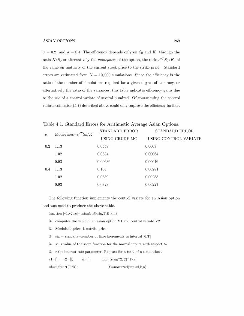
σ = 0.2 and σ = 0.4. The efficiency depends only on S0 and K through the
ratio K/S0 or alternatively the moneyness of the option, the ratio erTS0/K of
the value on maturity of the current stock price to the strike price. Standard
errors are estimated from N = 10, 000 simulations. Since the efficiency is the
ratio of the number of simulations required for a given degree of accuracy, or
alternatively the ratio of the variances, this table indicates efficiency gains due
to the use of a control variate of several hundred. Of course using the control
variate estimator (5.7) described above could only improve the efficiency further.
Table 4.1. Standard Errors for Arithmetic Average Asian Options.
σ Moneyness=erTS0/KSTANDARD ERROR
USING CRUDE MC
STANDARD ERROR
USING CONTROL VARIATE
0.2 1.13 0.0558 0.0007
1.02 0.0334 0.00064
0.93 0.00636 0.00046
0.4 1.13 0.105 0.00281
1.02 0.0659 0.00258
0.93 0.0323 0.00227
The following function implements the control variate for an Asian option
and was used to produce the above table.
function [v1,v2,sc]=asian(r,S0,sig,T,K,k,n)
% computes the value of an asian option V1 and control variate V2
% S0=initial price, K=strike price
% sig = sigma, k=number of time increments in interval [0.T]
% sc is value of the score function for the normal inputs with respect to
% r the interest rate parameter. Repeats for a total of n simulations.
v1=[]; v2=[]; sc=[]; mn=(r-sig^2/2)*T/k;
sd=sig*sqrt(T/k); Y=normrnd(mn,sd,k,n);

270 CHAPTER 5. SIMULATING THE VALUE OF OPTIONS
sc= (T/k)*sum(Y-mn)/(sd^2); Y=cumsum([zeros(1,n); Y]);
S = S0*exp(Y); v1= exp(-r*T)*max(mean(S)-K,0);
v2=exp(-r*T)*max(S0*exp(mean(Y))-K,0);
disp([’standard errors ’ num2str(sqrt(var(v1)/n)) ’ num2str(sqrt(var(v1-v2)/n))])
For example if we use K = 100, we might confirm the last row of the above
table using the command
asian(.1,100/1.1,.4,.2,100,50,10000);
Asian Options and Stratified Sampling
For many options, the terminal value of the stock has a great deal of influence
on the option price. Although it is difficult in general to stratify samples of
stock prices, it fairly easy to stratify along a single dimension, for example the
dimension defined by the stock price at time T. In particular we may stratify
the generation of
St = S0 exp(Zt)
where Zt can be written in terms of a standard Brownian motion
Zt = µt+ σWt, with µ = r − σ2/2.
To stratify into K strata of equal probability for ST we may generate ZT using
ZT = rT +prT − σ2T/2 Φ−1(i− 1 +
UiK), i = 1, 2, ...K
for Uniform[0,1] random variables Ui and then randomly generate the rest of the
path interpolating the value of S0 and ST using Brownian Bridge interpolation.
To do this we use the fact that for a standard Brownian motion and s < t < T
we have that the conditional distribution of Wt given Ws,WT is normal with
mean a weighted average of the value of the process at the two endpoints
T − t
T − sWs +
t− s
T − sWT

ASIAN OPTIONS 271
and variance(t− s)(T − t)
T − s.
Thus given the value of ST (or equivalently the value of W (T )) the increments
of the process at times ε, 2ε, ...N² = T say can be generated sequentially so
that the j’th increment W (jε) − W ((j − 1)ε) conditionally on the value of
W ((j − 1)ε) and of W (T ) has a Normal distribution with mean
(N − j
NW ((j − 1)ε) +
j
NW (T )
and with varianceN − j
N − j + 1.
Use of Girsanov’s Lemma.
There are many other variance reduction schemes that one can apply to valuing
an Asian Option. However prior to attacking this problem by other methods,
let us consider a simpler example.
Importance Sampling and Pricing a European Call Option
Suppose we wish to estimate the value of a call option using Monte Carlo meth-
ods which is well “out of the money”, one with a strike price K far above the
current price of the stock S0 so that if we were to attempt to evaluate this
option using crude Monte Carlo, the majority of the values randomly generated
for ST would fall below the strike and contribute zero to the option price. One
possible remedy is to generate values of ST under a distribution that is more
likely to exceed the strike, but of course this would increase the simulated value
of the option. We can compensate for changing the underlying distibution by
multiplying by a factor adjusting the mean as one does in importance sampling.
More specifically, we wish to estimate
EQ[e−rT (S0eZT −K)+], where ZT ∼ N(rT − σ2T/2,σ2T )

272 CHAPTER 5. SIMULATING THE VALUE OF OPTIONS
where EQ indicates that the expectation is taken under a risk neutral distri-
bution or probability measure Q for and K is large. Suppose that we modify
the underlying probability measure of ZT to Q0, say a normal distribution with
mean value ln(K/S0) − σ2T/2 but the same variance σ2T , then the expected
stock price under this new distribution
EQ0S0e
ZT = S0 exp(EQ0ZT + σ2T/2) = K
so there is a much greater probability that the strike price is attained. The
importance sampling adjustment that insures that the estimator continues to be
an unbised estimator of the option price is the ratio of two probability densities.
Denote the normal probability density function by
ϕ(x, µ,σ2) =1
√2πσ
exp{−(x− µ)2
2σ2}.
Then the Radon-Nikodym derivative
dQ
dQ0(zT ) =
ϕ(zt; rT −σ2T2 ,σ
2T )
ϕ(zt; ln(K/S0)−σ2T2 ,σ
2T )
is simply the ratio of the two normal density functions with the two different
means, and
EQ(e−rT (ST −K)+) = EQ0(e
−rT (ST −K)+dQ
dQ0(zT ))
= EQ0(e−rT (S0eZT −K)+
ϕ(ZT ; rT −σ2T2 ,σ
2T )
ϕ(ZT ; ln(K/S0)−σ2T2 ,σ
2T ))
so the importance sample estimator is the average of terms of the form
e−rT (S0eZT−K)+ϕ(ZT ; rT −
σ2T2 ,σ
2T )
ϕ(ZT ; ln(K/S0)−σ2T2 ,σ
2T ), where ZT ∼ N(ln(K/S0)−
σ2T
2,σ2T ).
The new simulation generates paths that are less likely to produce options ex-
piring with zero value, and in a sense has thus eliminated some computational
waste. What gains in efficiency result from this use of importance sampling?
Let us consider a three month (T = 0.25) call option with S0 = 10, K = 15,

ASIAN OPTIONS 273
σ = 0.2, r = .05. We determined the efficiency of the importance sampling es-
timator relative to using crude Monte Carlo in this situation using the function
below. Running this using the command [eff,m,v]=importance2(10,.05,15,.2,.25)
results in an efficiency gain of around 73, in part because very few of the crude
estimates of ST exceed the exercise price.
function [eff,m,v]=importance2(S0,r,K,sigma,T,N)
% simple importance sampling estimator of call option price
% outputs efficiency relative to crude. Run using
% [eff,m,v]=importance2(10,.05,15,.2,.25)
Z=randn(1,N);
%first do crude
ZT=(r-.5*sigma^2)*T+sigma*sqrt(T).*Z;
est1=exp(-r*T)*max(0,S0*exp(ZT)-K);
% now do importance
ZT=(log(K/S0)-.5*sigma^2)*T+sigma*sqrt(T).*Z;
ST=S0*exp(ZT);
est2=exp(-r*T)*max(0,ST-K).*normpdf(ZT,(r-.5*sigma^2)*T,sigma*sqrt(T))./normpdf(ZT,(log(K/S0)-
.5*sigma^2)*T,sigma*sqrt(T));
v=[var(est1) var(est2)];
m=[mean(est1) mean(est2)];
eff=v(1)/v(2);
Importance Sampling and Pricing an Asian Call Option
Let us now return to the price of an Asian option. We wish to use a variety
of variance reduction techniques including importance sampling as in the above
example, but in this case the relevant observation is not a simple stock price
at one instant but the whole stock price history from time 0 to T. An Asian
option to have a payoff related to the closing value of the stock S(T ). It might
274 CHAPTER 5. SIMULATING THE VALUE OF OPTIONS
be reasonable to stratify the sample; i.e. sample more often when S(T ) is large
or to use importance sampling and generate S(T ) from a geometric Brownian
motion with drift larger than rSt so that it is more likely that S(T ) > K. As
before if we do this we need to then multiply by the ratio of the two probability
density functions, or the Radon Nikodym derivative of one process with respect
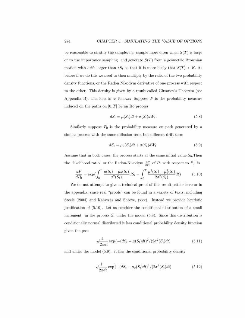
to the other. This density is given by a result called Girsanov’s Theorem (see
Appendix B). The idea is as follows: Suppose P is the probability measure
induced on the paths on [0, T ] by an Ito process
dSt = µ(St)dt+ σ(St)dWt. (5.8)
Similarly suppose P0 is the probability measure on path generated by a
similar process with the same diffusion term but different drift term
dSt = µ0(St)dt+ σ(St)dWt. (5.9)
Assume that in both cases, the process starts at the same initial value S0.Then
the “likelihood ratio” or the Radon-Nikodym dPdP0
of P with respect to P0 is
dP
dP0= exp{
Z T
0
µ(St)− µ0(St)
σ2(St)dSt −
Z T
0
µ2(St)− µ20(St)
2σ2(St)dt} (5.10)
We do not attempt to give a technical proof of this result, either here or in
the appendix, since real “proofs” can be found in a variety of texts, including
Steele (2004) and Karatzas and Shreve, (xxx). Instead we provide heuristic
justification of (5.10). Let us consider the conditional distribution of a small
increment in the process St under the model (5.8). Since this distribution is
conditionally normal distributed it has conditional probability density function
given the past
1√2πdt
exp{−(dSt − µ(St)dt)2/(2σ2(St)dt) (5.11)
and under the model (5.9), it has the conditional probability density
1√2πdt
exp{−(dSt − µ0(St)dt)2/(2σ2(St)dt) (5.12)

ASIAN OPTIONS 275
The ratio of these two probability density functions is
exp{µ(St)− µ0(St)
σ2(St)dSt −
µ2(St)− µ20(St)
2σ2(St)dt}
But the joint probability density function over a number of disjoint intervals is
obtained by multiplying these conditional densities together and this results in
Πt exp{µ(St)− µ0(St)
σ2(St)dSt −
µ2(St)− µ20(St)
2σ2(St)dt}
= exp{
Z T
0
µ(St)− µ0(St)
σ2(St)dSt −
Z T
0
µ2(St)− µ20(St)
2σ2(St)dt}
where the product of exponentials results in the sum of the exponents, or, in
the limit as the increment dt approaches 0, the corresponding integrals.
Girsanov’s result is very useful in conducting simulations because it permits
us to change the distribution under which the simulation is conducted. In
general, if we wish to determine an expected value under the measure P, we
may conduct a simulation under P0 and then multiply by dPdP0
or if we use a
subscript on E to denote the measure under which the expectation is taken,
EPV (ST ) = EP0 [V (ST )dP
dP0].
Suppose, for example, we wish to determine by simulation the expected value
of V (rT ) for an interest rate model
drt = µ(rt)dt+ σdWt (5.13)
for some choice of function µ(rt). Then according to Girsanov’s theorem, we
may simulate rt under the Brownian motion model drt = µ0dt+ σdWt (having
the same initial value r0 as in our original simulation) and then average the
values of
V (rT )dP
dP0= V (rT ) exp{
Z T
0
µ(rt)− µ0σ2
drt −
Z T
0
µ2(rt)− µ202σ2
dt} (5.14)
So far, the constant µ0 has been arbitrary and we are free to choose it in order
to achieve as much variance reduction as possible. Ideally we do not want to get

276 CHAPTER 5. SIMULATING THE VALUE OF OPTIONS
too far from the original process so µ0 should not be too far from the values of
µ(rt). In this case we hope that the term dPdP0
is not too variable (note that c dPdP0
would be the estimator if V (ST ) = c were constant). On the other hand, the
term V (rT ) cannot generally be ignored, and there is no formula or simple rule
for choosing parameters which minimize the variance of V (rT ) dPdP0 . Essentially
we need to resort to choosing µ0 to minimize the variance of V (rT ) dPdP0 by
experimentation, usually using with preliminary simulations.
Pricing a Call option under stochastic interest
rates.
(REVISE MODEL)Again we consider pricing a call option, but this time under
a more realistic model which permits stochastic interest rates. We will use
the method of conditioning, although there are many other potential variance
reduction tools here. Suppose the asset price, (under the risk-neutral probability
measure, say) follows a geometric Brownian motion model of the form
dSt = rtStdt+ σStdW(1)t (5.15)
where rt is the spot interest rate. We assume rt is stochastic and follows the
Brennan-Schwartz model,
drt = a(b− rt)dt+ σ0rtdW(2)t (5.16)
where W (1)t ,W
(2)t are both Brownian motion processes and usually assumed to
be correlated with correlation coefficient ρ. The parameter b in (5.16) can
be understood to be the long run average interest rate (the value that it would
converge to in the absence of shocks or resetting mechanisms) and the parameter
a > 0 governs how quickly reversion to b occurs.
It would be quite remarkable if a stock price is completely independent of
interest rates, since both will depend on an overlaping set of factors. However

PRICING A CALL OPTION UNDER STOCHASTIC INTEREST RATES.277
we begin by assuming something a little less demanding, that the random noise
processes driving the asset price and stock price are independent or that ρ = 0.
Control Variates.
The first method might be to use crude Monte Carlo; i.e. to simulate both the
process St and the process rt, evaluate the option at expiry, say V (ST , T ) and
then discount to its present value by multiplying by exp{−R T0rtdt}. However,
in this case we can exploit the assumption that ρ = 0 so that interest rates are
independent of the Brownian motion process W (1)t which drives the asset price
process. For example, suppose that the interest rate function rt were known
(equivalently: condition on the value of the interest rate process so that in the
conditional model it is known). While it may be difficult to obtain the value of
an option under the model (5.15), (5.16) it is usually much easier under a model
which assumes constant interest rate c. Let us call this constant interest rate
model for asset prices with the same initial price S0 and driven by the equation
dZt = cZtdt+ σZtdW(1)t , Z0 = S0 (5.17)
model “0” and denote the probability measure and expectations under this
distribution by P0 and E0 respectively. The value of the constant c will be
determined later. Assume that we simulated the asset prices under this model
and then valued a call option, say. Then since
ln(ZT /Z0) has a N((c−σ2
2)T,σ2T ) distribution
we could use the Black-Scholes formula to determine the conditional expected
value

278 CHAPTER 5. SIMULATING THE VALUE OF OPTIONS
E0[exp{−
Z T
0
rtdt}(ZT −K)+|rs, 0 < s < T ] (5.18)
= EE0[(S0e(c−r)T eW − e−rTK)+|rs, 0 < s < T ],
where W has a N(−σ2T/2,σ2T )
= E[BS(S0e(c−r)T ,K, r, T,σ)], with r =
1
T
Z T
0
rtdt.
Here, r is the average interest rate over the period and the function BS is
the Black-Scholes formula (5.2). In other words by replacing the interest rate
by its average over the period and the initial value of the stock by S0e(c−r)T ,
the Black-Scholes formula provides the value for an option on an asset driven
by (5.17) conditional on the value of r. The constant interest rate model is a
useful control variate for the more general model (5.16). The expected value
E[BS(S0e(c−r)T ,K, r, T,σ)] can be determined by generating the interest rate
processes and averaging values of BS(S0e(c−r)T ,K, r, T,σ). Finally we may es-
timate the required option price under (5.15),(5.16) using an average of values
of
exp{−
Z T
0
rtdt}[(ST −K)+ − (ZT −K)
+]}+E{BS(S0e(c−r)T ,K, r, T,σ)}
for ST and ZT generated using common random numbers.
We are still able to make a choice of the constant c. One simple choice is c ≈
E(r) since this means that the second term is approximatelyE{BS(S0,K, r, T,σ)}.
Alternatively we can again experiment with small numbers of test simulations
and various values of c in an effort to roughly minimize the variance
var(exp{−
Z T
0
rtdt}[(ST −K)+ − (ZT −K)
+]}).
Evidently it is fairly easy to arrive at a solution in the case ρ = 0 since
we really only need to average values of the Black Scholes price under various
randomly generated interest rates. This does not work in the case ρ 6= 0 because

SIMULATING BARRIER AND LOOKBACK OPTIONS 279
the conditioning involved in (5.18) does not result in the Black Scholes formula.
Nevertheless we could still use common random numbers to generate two interest
rate paths, one corresponding to ρ = 0 and the other to ρ 6= 0 and use the
former as a control variate in the estimation of an option price in the general
case.
Importance Sampling
The expectation under the correct model could also be determined by multiply-
ing this random variable by the ratio of the two likelihood functions and then
taking the expectation under E0. By Girsanov’s Theorem, E{V (ST , T )} =
E0{V (ST , T )dPdP0} where P is the measure on the set of stock price paths corre-
sponding to (5.15),(5.16) and P0 that measure corresponding to (5.17). The
required Radon-Nykodym derivative is
dP
dP0= exp{
Z T
0
(rt − c)StS2t σ
2dSt −
Z T
0
(r2t − c2)S2t
2σ2S2tdt} (5.19)
= exp{
Z T
0
rt − c
Stσ2dSt −
Z T
0
r2t − c2
2σ2dt} (5.20)
The resulting estimator of the value of the option is therefore an average
over all simulations of the value of
V (ST , T )exp{−
Z T
0
rtdt+
Z T
0
rt − c
σ2rtdSt −
Z T
0
r2t − c2
2σ2dt} (5.21)
where the trajectories rtare simulated under interest rate model (5.16).
As discussed before, we can attempt to choose the drift parameter c to
approximately minimize the variance of the estimator (5.21).
Simulating Barrier and lookback options
For a financial times series Xt observed over the interval 0 · t · T , what
is recorded in newspapers is often just the initial value or open of the time

280 CHAPTER 5. SIMULATING THE VALUE OF OPTIONS
series O = X0, the terminal value or close C = XT , the maximum over the
period or the high, H = max{Xt; 0 · t · T} and the minimum or the low
L = min{Xt; 0 · t · T}. Very few uses of the highly informative variables H
and L are made, partly becuase their distribution is a bit more complicated than
that of the normal distribution of returns. Intuitively, however, the difference
between H and L should carry a great deal of information about one of the
most important parameters of the series, its volatility. Estimators of volatility
obtained from the range of prices H −L or H/L will be discussed in Chapter 6.
In this section we look at how simple distributional properties of H and L can
be used to simulate the values of certain exotic path-dependent options.
Here we consider options such as barrier options, lookback options and hind-
sight options whose value function depends only on the four variables (O,H,L,C)
for a given process. Barrier options include knock-in and knock-out call options
and put options. Barrier options are simple call or put options with a fea-
ture that should the underlying cross a prescribed barrier, the option is either
knocked out (expires without value) or knocked in (becomes a simple call or
put option). Hindsight options, also called fixed strike lookback options are like
European call options in which we may use any price over the interval [0, T ]
rather than the closing price in the value function for the option. Of course for
a call option, this would imply using the high H and for a put the low L. A
few of these path-dependent options are listed below.
Option Payoff
Knock-out Call (C −K)+I(H · m)
Knock-in Call (C −K)+I(H ≥ m)
Look-back Put H − C
Look-Back Call C − L
Hindsight (fixed strike lookback) Call (H −K)+
Hindsight (fixed strike lookback) put (K − L)+
Table XX: Value Function for some exotic options
For further details, see Kou et. al. (1999) and the references therein.
SIMULATING BARRIER AND LOOKBACK OPTIONS 281
Simulating the High and the Close
All of the options mentioned above are functions of two or three variables O,C,
and H or O,C, and L and so our first challenge is to obtain in a form suitable
to calculation or simulation the joint distribution of these three variables. Our
argument will be based on one of the simplest results in combinatorial proba-
bility, the reflection principle. We would like to be able to handle more than
just a Black-Scholes model, both discrete and continuous distributions, and we
begin with the simple discrete case.
In the real world, the market does not rigorously observe our notions of the
passage of time. Volatility and volume traded vary over the day and by day
of the week. A successful model will permit some variation in clock speed and
volatility, and so we make an attempt to permit both in our discrete model.
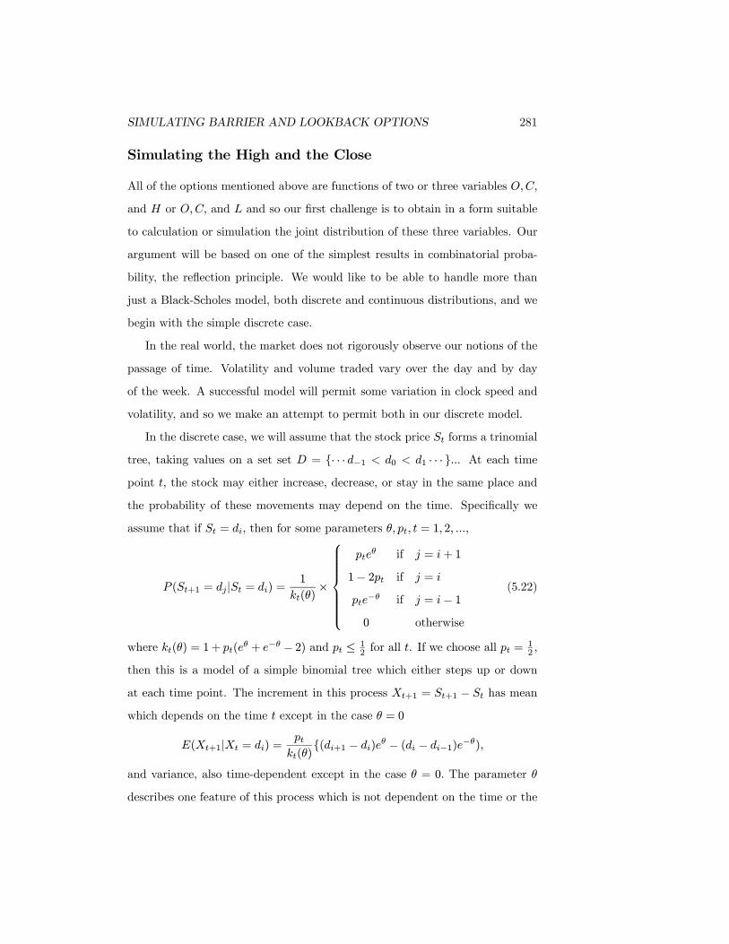
In the discrete case, we will assume that the stock price St forms a trinomial
tree, taking values on a set set D = {· · · d−1 < d0 < d1 · · · }... At each time
point t, the stock may either increase, decrease, or stay in the same place and
the probability of these movements may depend on the time. Specifically we
assume that if St = di, then for some parameters θ, pt, t = 1, 2, ...,
P (St+1 = dj |St = di) =1
kt(θ)×
⎧⎪⎪⎪⎪⎪⎪⎨⎪⎪⎪⎪⎪⎪⎩
pteθ if j = i+ 1
1− 2pt if j = i
pte−θ if j = i− 1
0 otherwise
(5.22)
where kt(θ) = 1+ pt(eθ + e−θ − 2) and pt · 12 for all t. If we choose all pt =
12 ,
then this is a model of a simple binomial tree which either steps up or down
at each time point. The increment in this process Xt+1 = St+1 − St has mean
which depends on the time t except in the case θ = 0
E(Xt+1|Xt = di) =ptkt(θ)
{(di+1 − di)eθ − (di − di−1)e−θ),
and variance, also time-dependent except in the case θ = 0. The parameter θ
describes one feature of this process which is not dependent on the time or the

282 CHAPTER 5. SIMULATING THE VALUE OF OPTIONS
Figure 5.1: Illustration of the Reflection Principle
location of the process, since the log odds of a move up versus a move down is
2θ = log[P [UP]
P [DOWN]].
Now suppose we label the states of the process so that S0 = d0 and there is
a barrier at the point dm where m > 0. We wish to count the number of paths
over an interval of time [0, T ] which touch or cross this barrier and end at a
particular point du, u < m. Such a path is shown as a solid line in Figure 5.1 in
the case that the points di are all equally spaced. Such a path has a natural
“reflection” about the horizontal line at dm. The reflected path is identical up
to the first time τ that the original path touches the point dm, and after this
time, say at time t > τ, the relected path takes the value d2m−i where St = di.
This path is the dotted line in Figure 5.1. Notice that if the original path ends
at du < dm, below the barrier, the reflected path ends at d2m−u > dm or above
the barrier. Each path touching the barrier at least once and ending below it
at du has a reflected path ending above it at d2m−u, and of course each path
that ends above the barrier must touch the barrier for a first time at some point
and has a reflection that ends below the barrier. This establishes a one-one
correspondence useful for counting these paths. Let us denote by the symbol

SIMULATING BARRIER AND LOOKBACK OPTIONS 283
“#” the “number of paths such that”. Then:
#{H ≥ dm and C = du < dm} = #{C = d2m−u}.
Now consider the probability of any path ending at a particular point du,
(S0 = d0, S1, ..., ST = du).
To establish this probability, each time the process jumps up in this interval
we must multiply by the factor pteθ
kt(θ)and each time there is a jump down we
multiply by pte−θ
kt(θ). If the process stays in the same place we multiply by 1−2pt
kt(θ).
The reflected path has exactly the same factors except that after the time τ at
which the barrier is touched, the “up” jumps are replaced by “down” jumps and
vice versa. For an up jump in the original path multiply by e−2θ. For a down
jump in the original path, multiply by e2θ. Of course this allows us to compare
path probabilities for an arbitrary value of the parameter θ, say with P0, the
probability under θ = 0 since, if the path ends at C = du,
Pθ(path) =eNUθe−NDθQ
t kt(θ)P0[path]
=euθQt kt(θ)
P0[path] (5.23)
where NU and ND are the number of up jumps and down jumps in the path.
Note that we have subscripted the probability measure by the assumed value of
the parameter θ.
This makes it easy to compare the probabilities of the original and the re-
flected path, since
Pθ[original path]Pθ[reflected path]
= e−2θNU e2θND
where now the number of up and down jumps NU and ND are counted following
time τ. However, since ST = du and Sτ = dm, it follows that ND−NU = m−u
and thatP [original path]P [reflected path]
= e2θ(u−m)
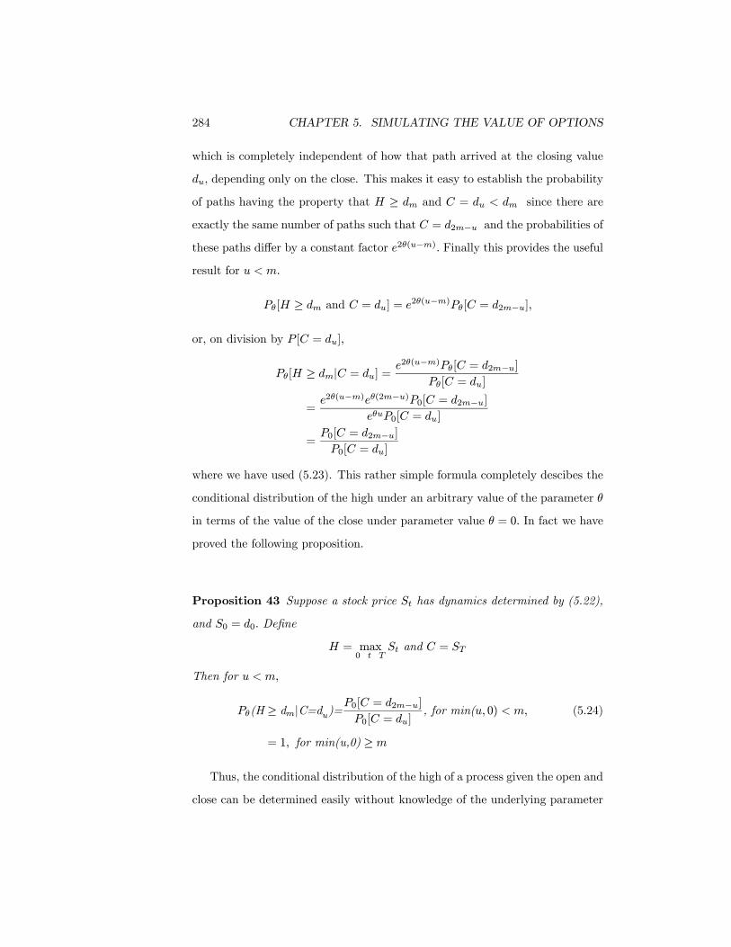
284 CHAPTER 5. SIMULATING THE VALUE OF OPTIONS
which is completely independent of how that path arrived at the closing value
du, depending only on the close. This makes it easy to establish the probability
of paths having the property that H ≥ dm and C = du < dm since there are
exactly the same number of paths such that C = d2m−u and the probabilities of
these paths differ by a constant factor e2θ(u−m). Finally this provides the useful
result for u < m.
Pθ[H ≥ dm and C = du] = e2θ(u−m)Pθ[C = d2m−u],
or, on division by P [C = du],
Pθ[H ≥ dm|C = du] =e2θ(u−m)Pθ[C = d2m−u]
Pθ[C = du]
=e2θ(u−m)eθ(2m−u)P0[C = d2m−u]
eθuP0[C = du]
=P0[C = d2m−u]P0[C = du]
where we have used (5.23). This rather simple formula completely descibes the
conditional distribution of the high under an arbitrary value of the parameter θ
in terms of the value of the close under parameter value θ = 0. In fact we have
proved the following proposition.
Proposition 43 Suppose a stock price St has dynamics determined by (5.22),
and S0 = d0. Define
H = max0� t�T
St and C = ST
Then for u < m,
Pθ(H ≥ dm|C=du)=P0[C = d2m−u]P0[C = du]
, for min(u, 0) < m, (5.24)
= 1, for min(u,0) ≥ m
Thus, the conditional distribution of the high of a process given the open and
close can be determined easily without knowledge of the underlying parameter

SIMULATING BARRIER AND LOOKBACK OPTIONS 285
and is related to the distribution of the close when the “drift” θ = 0. This result
also gives the expected value of the high in fairly simple form if the points dj are
equally spaced. Suppose dj = j∆ for j = 0,±1,±2, .... Then for u = j∆,with
j ≥ 0 and k ≥ 1, (see Problem 1)
Pθ[H − C ≥ k∆|C = j∆] =
E[H |C = u] = u+∆P [C > u and C−u
∆ is even]P [C = u]
.
Roughly, (5.24) indicates that if you can simulate the close under θ, then
you use the properties of the close under θ = 0 to simulate the high of the
process. Consider the problem of simulating the high for a given value of the
close C = ST = du and again assuming that S0 = d0. Suppose we use inverse
transform from a uniform random variable U to solve the inequalities
Pθ( max0� t�T
St ≥ dm+1|ST = du) < U · Pθ( max0� t�T
St ≥ dm|ST = du)
for the value of dm. In this case the value of
dm = sup{dj ;UP0[ST = du] · P0[ST = d2j−u]}
is the generated value of the high. This inequality is equivalent to
P0[ST = d2m+2−u] < UP0[ST = du] · P0[ST = d2m−u].
Graphically this inequality is demonstrated in Figure 5.2 which shows the prob-
ability histogram of the distribution ST under θ = 0. The value UP0[ST = du]
is the y-coordinate of a point P randomly chosen from the bar corresponding
to the point du. The high dm is generated by moving horizontally to the right
an even number of steps until just before exiting the histogram. This is above
the value d2m−u and dm is between du and d2m−u.
A similar result is available for Brownian motion and Geometric Brownian
motion. A justification of these results can be made by taking a limit in the

286 CHAPTER 5. SIMULATING THE VALUE OF OPTIONS
Figure 5.2: Generating a High, discrete distributions
discrete case as the time steps and the distances dj − dj−1 all approach zero. If
we do this, the parameter θ is analogous to the drift of the Brownian motion.
The result for Brownian motion is as follows:
Theorem 44 Suppose St is a Brownian motion process
dSt = µdt+ σdWt,
S0 = 0, ST = C,
H = max{St; 0 · t · T} and
L = min{St; 0 · t · T}.
If f0 denotes the Normal(0,σ2T ) probability density function, the distribution of
C under drift µ = 0, then
UH =f0(2H − C)
f0(C)is distributed as U [0, 1] independently of C,
UL =f0(2L− C)
f0(C)is distributed as U [0, 1] independently of C.
ZH = H(H − C) is distributed as Exponential (1
2σ2T ) independently of C,
ZL = L(L− C) is distributed as Exponential (1
2σ2T )independently of C.
We will not prove this result since it is a special case of Theorem 46 below.
However it is a natural extension of Proposition 43 in the special case that

SIMULATING BARRIER AND LOOKBACK OPTIONS 287
dj = j∆ for some ∆ and so we will provide a simple sketch of a proof using
this proposition. Consider the ratio
P0[C = d2m−u]P0[C = du]
on the right side of (5.24). Suppose we take the limit of this as ∆ → 0 and as
m∆→ h and u∆→ c. Then this ratio approaches
f0(2h− c)
f0(c)
where f0 is the probability density function of C under µ = 0. This implies for
a Brownian motion process,
P [H ≥ h|C = c] =f0(2h− c)
f0(c)for h ≥ c. (5.25)
If we temporarily denote the cumulative distribution function of H given C = c
by Gc(h) then (5.25) gives an expression for 1 − Gc(h) and recall that since
the sumulative distribution function is continuous, when we evaluate it at the
observed value of a random variable we obtain a U [0, 1] random variable e.g.
Gc(H) ∼ U [0, 1]. In other words conditional on C = c we have
f0(2H − c)
f0(c)∼ U [0, 1].
This result verifies a simple geometric procedure, directly analogous to that in
Figure 5.2, for generating H for a given value of C = c. Suppose we gener-
ate a point PH = (c, y) under the graph of f0(x) and uniformly distributed
on {(c, y); 0 · y · f0(c)}. This point is shown in Figure ??. We regard the
y−coordinate of this point as the generated value of f0(2H− c). Then H can be
found by moving from PH horizontally to the right until we strike the graph of
f0 and then moving vertically down to the axis (this is now the point 2H − c)
and finally taking the midpoint between this coordinate 2H − c and the close
c to obtain the generated value of the high H. The low of the process can be
generated in the same way but with a different point PL uniform on the set

288 CHAPTER 5. SIMULATING THE VALUE OF OPTIONS
Figure 5.3: Generating H for a fixed value of C for a Brownian motion.
{(c, y); 0 · y · f0(c)}. The algorithm is the same in this case except that we
move horizontally to the left.
There is a similar argument for generating the high under a geometric Brown-
ian motion as well, since the logarithm of a geometric Brownian motion is a
Brownian motion process.
Corollary 45 For a Geometric Brownian motion process
dSt = µStdt+ σStdWt,
S0 = O and ST = C
with f0 the normal(0,σ2T ) probability density function, we have
ln(H/O) ln(H/C) ∼ exp(1
2σ2T ) independently of O,C and
ln(L/O) ln(L/C) ∼ exp(1
2σ2T ) independently of O,C.
UH =f0(ln(H
2/OC))
f0(ln(C/O))∼ U [0, 1] independently of O,C and
UL =f0(ln(L
2/OC))
f0(ln(C/O))∼ U [0, 1] independently of O,C.

SIMULATING BARRIER AND LOOKBACK OPTIONS 289
Both of these results are special cases of the following more general Theorem.
We refer to McLeish(2002) for the proof. As usual, we consider a price process
St and define the high H = max{St; 0 · t · T}, and the open and close O = S0,
C = ST .
Theorem 46 Suppose the process St satisfies the stochastic differential equa-
tion:
dSt = {ν +1
2σ0(St)}σ(St)λ2(t)dt+ σ(St)λ(t)dWt (5.26)
where σ(x) > 0 and λ(t) are positive real-valued functions such that g(x) =R x 1σ(y)dy and θ =
R T0λ2(s)ds <∞ are well defined on <+.
(a) Then with f0 the N(0, θ) probability density function we have
UH =f0{2g(H)− g(O)− g(C)}
f0{g(C)− g(O)}∼ U [0, 1]
and UH is independent of C.
(b) For each value of T , ZH = (g(H) − g(O))(g(H) − g(C)) is independent of
O,C, and has an exponential distribution with mean 12θ.
A similar result holds for the low of the process over the interval, namely
that
UL =f0{2g(L)− g(O)− g(C)}
f0{g(C)− g(O)}∼ U [0, 1]
and ZH = {g(L) − g(O)}{g(L) − g(C)} is independent of O,C, and has an
exponential distribution with mean 12θ.
Before we discuss the valuation of various options, we examing the signif-
icance of the ratio appearing in on the right hand side of (5.25) a little more
closely. Recall that f0 is the N(0,σ2T ) probability density function and so we
can replace it by
f0(2h− c)
f0(c)=exp{− (2h−c)2
2σ2T }
exp{− c2
2σ2T }= exp{−2
zhσ2T
} (5.27)
290 CHAPTER 5. SIMULATING THE VALUE OF OPTIONS
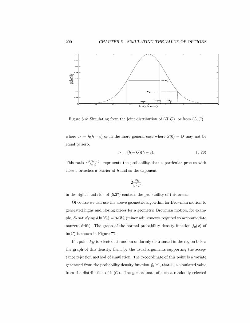
Figure 5.4: Simulating from the joint distribution of (H,C) or from (L,C)
where zh = h(h − c) or in the more general case where S(0) = O may not be
equal to zero,
zh = (h− O)(h− c). (5.28)
This ratio f0(2h−c)f0(c)
represents the probability that a particular process with
close c breaches a barrier at h and so the exponent
2zhσ2T
in the right hand side of (5.27) controls the probability of this event.
Of course we can use the above geometric algorithm for Brownian motion to
generated highs and closing prices for a geometric Brownian motion, for exam-
ple, St satisfying d ln(St) = σdWt (minor adjustments required to accommodate
nonzero drift). The graph of the normal probability density function f0(x) of
ln(C) is shown in Figure ??.
If a point PH is selected at random uniformly distributed in the region below
the graph of this density, then, by the usual arguments supporting the accep-
tance rejection method of simulation, the x-coordinate of this point is a variate
generated from the probability density function f0(x), that is, a simulated value
from the distribution of ln(C). The y-coordinate of such a randomly selected

SIMULATING BARRIER AND LOOKBACK OPTIONS 291
point also generates the value of the high as before.If we extend a line horizon-
tally to the right from PH until it strikes the graph of the probability density and
then consider the abscissa, of this point, this is the simulated value of ln(H2/C),
and ln(H) the average the simulated values of ln(H2/C) and ln(C).
A similar point PL uniform under the probability density function f0 can be
used to generate the low of the process if we extend the line from PL to the left
until it strikes the density. Again the abscissa of this point is ln(L2/C) and the
average with ln(C) gives a simulated value of ln(L). Although the y−coordinate
of both PH and PL are uniformly distributed on [0, f0(C)] conditional on the
value of C they are not independent.
Suppose now we wish to price a barrier option whose payoff on maturity
depends on the value of the close C but provided that the high H did not
exceed a certain value, the barrier. This is an example of an knock-out barrier
but other types are similarly handled. Once again we assume the simplest form
of the geometric Brownian motion d ln(St) = σdWt and assume that the upper
barrier is at the point Oeb so that the payoff from the option on maturity T is
ψ(C)I(H < Oeb)
for some function ψ. It is clear that the corresponding value of H does not
exceed a boundary at Oeb if and only if the point PH is below the graph of the
probability density function but not in the shaded region obtained by reflecting
the right hand tail of the density about the vertical line x = b − ln(O) in
Figure 5.5. To simulate the value of the option, choose points uniformly under
the graph of the probability density f0(x). For those points in the non-shaded
region under f0 (the x-coordinate of these points are simulated values ψ(C)of
ln(C) under the condition that the barrier is not breached) we average the values
of ψ(C) and for those in the shaded region we average 0.
Equivalently,
Eψ(C)I(H < Oeb) = Eψ∗(C)

292 CHAPTER 5. SIMULATING THE VALUE OF OPTIONS
Figure 5.5: Simulating a knock-out barrier option with barrier at Oeb
where
ψ∗(C) =
⎧⎨⎩ ψ(C) for C · Oeb
−ψ(2b+ ln(O2/C)) for C > Oeb.
and so the barrier option can be priced as if it were a vanilla European option
with payoff function ψ∗(C).
Any option whose value depends on the high and the close of the process
(or (L,C)) can be similarly valued as a European option. If an option be-
comes worthless whenever an upper boundary at Oeb is breached, we need only
multiply the payoff from the option ignoring the boundary by the factor
1− exp{−2zhσ2T
}
with
zh = b(b+ ln(O/C))
to accommodate the filtering effect of the barrier and then value the option as
if it were a European option.
There is a a variety of distributional results related to H, some used by
Redekop (1995) to test the local Brownian nature of various financial time series.
These are easily seen in Figure 5.7. For example, for a Brownian motion process

SIMULATING BARRIER AND LOOKBACK OPTIONS 293
-4 -3 -2 -1 0 1 2 3 40
0.05
0.1
0.15
0.2
0.25
0.3
0.35
0.4
ln(C)
prob
abili
ty
ln(O) m
PH•
Figure 5.6: Simulating a Barrier Option with barrier at em
with sero drift, suppose we condition on the value of 2H − O − C. Then the
point PH must lie (uniformly distributed) on the line L1 and therefore the point
H lies uniformly on this same line but to the right of the point O. This shows
that conditional on 2H − O − C the random variable H − O is uniform or,
H − O
2H − O − C∼ U [0, 1].
Similarly, conditional on the value of H, the point PH must fall somewhere on
the curve labelled C2 whose y-coordinate is uniformly distributed showing that
C − O
2H − O − C∼ U [0, 1].
Redekop shows that for a Brownian motion process, the statistic
H − O
2H − O − C(5.29)
is supposed to be uniformly [0, 1] distributed but when evaluated using real
financial data, is far too often close to or equal the extreme values 0 or 1.

294 CHAPTER 5. SIMULATING THE VALUE OF OPTIONS
Figure 5.7: Some uniformly distributed statistics for Brownian Motion
The joint distribution of (C,H) can also be seen from Figure 5.8. Note
that the rectangle around the point (x, y) of area ∆x∆y under the graph of the
density, when mapped into values of the high results in an interval of values for
(2H − C) of width −∆y/φ0(2y − x) where φ0 is the derivative of the standard
normal probability density function (the minus sign is to adjust for the negative
slope of the density here). This interval is labelled ∆(2H − C). This, in turn
generates the interval ∆H of possible values of H, of width exactly half this, or
−∆y
2φ0(2y − x).
Inverting this relationship between (x, y) and (H,C),
P [H ∈ ∆H,C ∈ ∆C] = −2φ0(2y − x)∆x∆y
confirming that the joint density of (H,C) is given by −2φ0(2y − x) for x < y.
In order to get the joint density of the High and the Close when the drift is
non-zero, we need only multiply by the ratio of the two normal density functions
of the closefµ(x)
f0(x)

SIMULATING BARRIER AND LOOKBACK OPTIONS 295
Figure 5.8: Confirmation of the joint density of (H,C)
and this gives the more general result in the table below.
The table below summarizes many of our distributional results for a Brown-
ian motion process with drift on the interval [0, 1],
dSt = µdt+ σdWt, with S0 = O.
Statistic Density Conditions
X = C − O,
Y = H − Of(y, x) = −2φ0(2y − x) exp(µx− µ2/2)
−∞ < x < y,
and y > 0,σ = 1
given O
Y |X fY |X(y|x) = 2(2y − x)e−2y(y−x) y > x,σ = 1
Z = Y (Y −X) exp((σ2/2) given O,X
(L− O)(L− C) exp(σ2/2) given (O,C)
(H − O)(H − C) exp(σ2/2) given (O,C)
H−O2H−O−C U [0, 1] drift ν = 0, given O, 2H − O − C
L−O2L−O−C U [0, 1] drift ν = 0, given O, 2L− O − C
C−O2H−O−C U [−1, 1] drift ν = 0, given H,O
TABLE 5.1: Some distributional results for High, Close and Low.

296 CHAPTER 5. SIMULATING THE VALUE OF OPTIONS
We now consider briefly the case of non-zero drift for a geometric Brownian
motion. Fortunately, all that needs to be changed in the results above is the
marginal distribution of ln(C) since all conditional distributions given the value
of C are the same as in the zero-drift case. Suppose an option has payoff on
maturity ψ(C) if an upper barrier at level Oeb, b > 0 is not breached. We have
already seen that to accommodate the filetering effect of this knock-out barrier
we should determine, numerically or by simulation, the expected value
E[ψ(C)(1− exp{−2b(b+ ln(O/C))
σ2T})]
the expectation conditional (as always) on the value of the open O. The effect
of a knock-out lower barrier at Oe−a is essentially the same but with b replaced
by a, namely
E[ψ(C)(1− exp{−2a(a+ ln(C/O))
σ2T})].
In the next section we consider the effect of two barriers, both an upper and a
lower barrier.
One Process, Two barriers.
We have discussed a simple device above for generating jointly the high and the
close or the low and the close of a process given the value of the open. The joint
distribution of H,L,C given the value of O or the distribution of C in the case
of upper and lower barriers is more problematic. Consider a single factor model
and two barriers- an upper and a lower barrier. Note that the high and the
low in any given interval is dependent, but if we simulate a path in relatively
short segments, by first generating n increments and then generating the highs
and lows within each increment, then there is an extremely low probability
that the high and low of the process will both lie in the same short increment.
For example for a Brownian motion with the time interval partitioned into 5
equal subintervals, the probability that the high and low both occur in the
SIMULATING BARRIER AND LOOKBACK OPTIONS 297
same increment is less than around 0.011 whatever the drift. If we increase the
number of subintervals to 10, this is around 0.0008. This indicates that provided
we are willing to simulate highs, lows and close in ten subintervals, pretending
that within subintervals the highs and lows are conditionally independent, the
error in our approximation is very small.
An alternative, more computationally intensive, is to differentiate the infinite
series expression for the probability P (H · b, L ≥ a,C = u|O = 0] A first step
in this direction is the the following result, obtained from the reflection principle
with two barriers.
Theorem 47 For a Brownian motion process
dSt = µdt+ dWt, S0 = 0
defined on [0, 1] and for −a < u < b,
P (L < −a or H > b|C = u)
=1
φ(u)
∞Xn=1
[φ{2n(a+ b) + u}+ φ{2n(a+ b)− 2a− u}
+ φ{−2n(b+ a) + u}+ φ{2n(b+ a) + 2a+ u}]
where φ is the N(0, 1) probability density function.
Proof. The proof is a well-known application of the reflection principal.
It is sufficient to prove the result in the case µ = 0 since the conditional
distribution of L,H given C does not depend on µ (A statistician would say
that C is a sufficient statistic for the drift parameter). Denote the following
paths determined by their behaviour on 0 < t < 1. All paths are assumed to
end at C = u.

298 CHAPTER 5. SIMULATING THE VALUE OF OPTIONS
A+1 = H > b (path goes above b)
A+2 = path goes above b and then falls below −a
A+3 = goes above b then falls below −a then rises above b
etc.
A−1 = L < −a
A−2 = path falls below −a then rises above b
A−3 = falls below −a then rises above b then falls below −a
etc.For an arbitrary event A, denote by P (A|u) probability of the event conditional
on C = u. Then according to the reflection principal the probability that the
Brownian motion leaves the interval [−a, b] is given from an inclusion-exclusion
argument by
P (A+1|u)− P (A+2|u) + P (A+3|u)− · · · (5.30)
+P (A−1|u)− P (A−2|u) + P (A−3|u) · · ·
This can be verified by considering the paths in Figure 5.9. (It should be noted
here that, as in our application of the reflection principle in the one-barrier case,
the reflection principle allows us to show that the number of paths in two sets is
the same, and this really only translates to probability in the case of a discrete
sample space, for example a simple random walk that jumps up or down by a
fixed amount in discrete time steps. This result for Brownian motion obtains if
we take a limit over a sequence of simple random walks approaching a Brownian
motion process.)
Note that
P (A+1|u) =φ(2b− u)
φ(u)
P (A+2n|u) =φ{2n(a+ b) + u}
φ(u)
P (A+(2n−1)|u) =φ{2n(a+ b)− 2a− u}
φ(u)

SIMULATING BARRIER AND LOOKBACK OPTIONS 299
Figure 5.9: The Reflection principle with Two Barriers
and
P (A−1|u) =φ(−2a− u)
φ(u)
P (A−2n|u) =φ{−2n(b+ a) + u}
φ(u)
P (A−(2n+1)|u) =φ{2n(b+ a) + 2a+ u}
φ(u).
The result then obtains from substitution in (5.30).
As a consequence of this result we can obtain an expression for P (a < L ·
H < b, u < C < v) (see also Billingsley, (1968), p. 79) for a Brownian motion
on [0, 1] with zero drift:
P (a, b, u, v) = P (a < L · H < b, u < C < v)
=∞X
k=−∞Φ[v + 2k(b− a)]− Φ[u+ 2k(b− a)]
−∞X
k=−∞Φ[2b− u+ 2k(b− a)]− Φ[2b− v + 2k(b− a)]. (5.31)

300 CHAPTER 5. SIMULATING THE VALUE OF OPTIONS
where Φ is the standard normal cumulative distribution function. From (5.31)
we derive the joint density of (L,H,C) by taking the limit P (a, b, u, u+ δ)/δ as
δ → 0, and taking partial derivatives with respect to a and b:
f(a, b, u) = 4∞X
k=−∞k2φ00[u+ 2k(b− a)]− k(1 + k)φ00[2b− u+ 2k(b− a)]
= 4∞Xk=1
k2φ00[u+ 2k(b− a)]− k(1 + k)φ00[2b− u+ 2k(b− a)]
+ k2φ00[u− 2k(b− a)] + k(1− k)φ00[2b− u− 2k(b− a)] (5.32)
for a < u < b.
From this it is easy to see that the conditional cumulative distribution func-
tion of L given C = u,H = b is given by on a · u · b (where −2φ0(2b − u)
is the joint p.d.f. of H,C) by
F (a|b, u) = 1 +∂2
∂b∂vP (a, b, u, v)|v=u2φ0(2b− u)
(5.33)
=−1
φ0(2b− u)
∞Xk=1
{−kφ0[u+ 2k(b− a)] + (1 + k)φ0[2b− u+ 2k(b− a)]
+ kφ0[u− 2k(b− a)] + (1− k)φ0[2b− u− 2k(b− a)]}
This allows us to simulate both the high and the low, given the open and the
close by first simulating the high and the close using −2φ0(2b− u) as the joint
p.d.f. of (H,C) and then simulating the low by inverse transform from the
cumulative distribution function of the form (5.33).
Survivorship Bias
It is quite common for retrospective studies in finance, medicine and to be
subject to what is often called “survivorship bias”. This is a bias due to the
fact that only those members of a population that remained in a given class
(for example the survivors) remain in the sampling frame for the duration of
the study. In general, if we ignore the “drop-outs” from the study, we do so

SURVIVORSHIP BIAS 301
at risk of introducing substantial bias in our conclusions, and this bias is the
survivorship bias.
Suppose for example we have hired a stable of portfolio managers for a large
pension plan. These managers have a responsibility for a given portfolio over
a period of time during which their performance is essentially under continuous
review and they are subject to one of several possible decisions. If returns below
a given threshhold, they are deemed unsatisfactory and fired or converted to
another line of work. Those with exemplary performance are promoted, usually
to an administrative position with little direct financial management. And those
between these two “absorbing” barriers are retained. After a period of time,
T, an amibitious graduate of an unnamed Ivey league school working out of
head office wishes to compare performance of those still employed managing
portfolios. How are should the performance measures reflect the filtering of
those with unusually good or unusually bad performance? This is an example
of a process with upper and lower absorbing barriers, and it is quite likely
that the actual value of these barriers differs from one employee to another, for
example the son-in-law of the CEO has a substantially different barriers than the
math graduate fresh out of UW. However, let us ignore this difference, at least
for the present, and concentrate on a difference that is much harder to ignore
in the real world, the difference between the volatility parameters of portfolios,
possibly in different sectors of the market, controlled by different managers.
For example suppose two managers were responsible for funds that began and
ended the year at the same level and had approximately the same value for the
lower barrier as in Table 5.2. For each the value of the volatility parameter
σ was estimated using individual historical volatilities and correlations of the
component investments.

302 CHAPTER 5. SIMULATING THE VALUE OF OPTIONS
Portfolio Open price Close Price Lower Barrier Volatility
1 40 5658 30 .5
2 40 5614 30 .2
Table 5.2
Suppose these portfolios (or their managers) have been selected retrospec-
tively from a list of “survivors” which is such that the low of the portfolio value
never crossed a barrier at l = Oe−a (bankruptcy of fund or termination or
demotion of manager, for example) and the high never crossed an upper barrier
at h = Oeb. However, for the moment let us assume that the upper barrier is so
high that its influence can be neglected, so that the only absorbtion with any
substantial probability is at the lower barrier. We interested in the estimate of
return from the two portfolios, and a preliminary estimate indicates a continu-
ously compounded rate of return from portfolio 1 of R1 = ln(56.625/40) = 35%
and from portfolio two of R2 = ln(56.25/40) = 34%. Is this difference significant
and are these returns reasonably accurate in view of the survivorship bias?
We assume a geometric Brownian motion for both portfolios,
dSt = µStdt+ σStdWt, (5.34)
and define O = S(0), C = S(T ),
H = max0� t�T
S(t), L = min0� t�T
S(t)
with parameters µ,σ possibly different.
In this case it is quite easy to determine the expected return or the value of
any performance measure dependent on C conditional on survival, since this is
essentially the same as a problem already discussed, the valuation of a barrier
option. According to (5.27), the probability that a given Brownian motion
process having open 0 and close c strikes a barrier placed at l < min(0, c) is
exp{−2zlσ2T
}

SURVIVORSHIP BIAS 303
with
zl = l(l − c).
Converting this statement to the Geometric Brownian motion (5.34), the prob-
ability that a geometric Brownian motion process with open O and close c
breaches a lower barrier at l is
P [L · l|O,C] = exp{−2zlσ2T
}
with
zl = ln(O/l) ln(C/l) = a(a+ ln(C/O)).
Of course the probability that a particular path with this pair of values (O,C)
is a “survivor” is 1 minus this or
1− exp{−2zlσ2T
}. (5.35)
When we observe the returns or the closing prices C of survivors only, the results
have been filtered with probability (5.35). In other words if the probability
density function of C without any barriers at all is f(c) (in our case this is a
lognormal density with parameters that depend on µ and σ) then the density
function of C of the survivors in the presence of a lower barrier is proportional
to
f(c)[1− exp{−2ln(O/l) ln(c/l)
σ2T}]
= f(c)(1− (l
c)λ), with λ =
2 ln(O/l)
σ2T=
2a
σ2T> 0.
It is interesting to note the effect of this adjustment on the moments of C for
various values of the parameters. For example consider the expected value of C
conditional on survival
E(C|L ≥ l] =
R∞lcf(c)(1− ( lc)
λ)dcR∞lf(c)(1− ( lc)
λ)dc
=E[CI(C ≥ l)]− lλE[C1−λI(C ≥ l)]P [C ≥ l]− lλE[C−λI(C ≥ l)]
(5.36)

304 CHAPTER 5. SIMULATING THE VALUE OF OPTIONS
and this is easy to evaluate in the case of interest in which C has a lognormal
distribution. In fact the same kind of calculation is used in the development of
the Black-Scholes formula. In our case C = exp(Z) where Z is N(µT,σ2T )
and so for any p and l > 0, we have from (3.11), using the fact that E(C |O) =
O exp{µT + σ2T/2}, (and assuming O is fixed),
E[CpI(C > l)] = Opexp{pµT + p2σ2T/2}Φ(1
σ√T(a+ µT ) + σ
√Tp)
To keep things slightly less combersome, let us assume that we observe the
geometric Brownian motion for a period of T = 1. Then (5.36) results in
Oeµ+σ2/2Φ( 1σ (a+ µ) + σ)− Oe−aλ+(1−λ)µ+(1−λ)
2σ2/2Φ( 1σ (a+ µ) + σ(1− λ))
Φ( 1σ (a+ µ))− e−λa−λµ+λ2σ2/2Φ( 1σ (a+ µ)− σλ)
Let there be no bones about it. At first blush this is still a truly ugly and
opaque formula. We can attempt to beautify it by re-expressing it in terms more
like those in the Black-Scholes formula, putting
d2(λ) =1
σ(µ− a), and d2(0) =
1
σ(a+ µ),
d1(λ) = d2(λ) + σ, d1(0) = d2(0) + σ.
These are analogous to the values of d1,d2 in the Black-Scholes formula in the
case λ = 0. Then
E[C|L ≥ l] = Oeµ+σ
2/2Φ(d1(0))− e−λa+(1−λ)µ+(1−λ)2σ2/2Φ(d1(λ))
Φ(d2(0))− e−λa−λµ+λ2σ2/2Φ(d2(λ))
. (5.37)
What is interesting is how this conditional expectation, the expected close for
the survivors, behaves as a function of the volatility parameter σ. Although this
is a rather complicated looking formula, we can get a simpler picture (Figure
5.10) using a graph with the drift parameter µ chosen so that E(C) = 56.25
is held fixed. We assume a = − ln(30/40) (consistent with Table 5.2)and vary
the value of σ over a reasonable range from σ = 0.1 (a very stable investment)
through σ = .8 (a highly volatile investment). In Figure 5.10 notice that for
small volatility, e.g. for σ · 0.2, the conditional expectation E[C|L ≥ 30]
SURVIVORSHIP BIAS 305
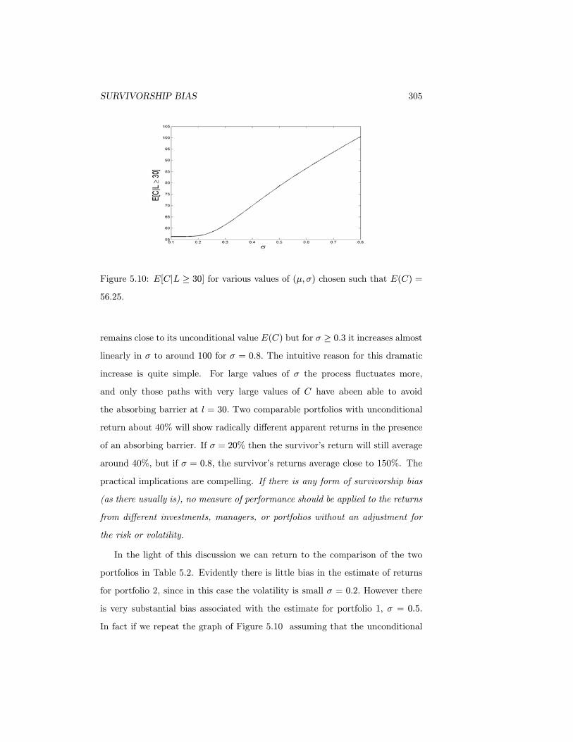
Figure 5.10: E[C |L ≥ 30] for various values of (µ,σ) chosen such that E(C) =
56.25.
remains close to its unconditional value E(C) but for σ ≥ 0.3 it increases almost
linearly in σ to around 100 for σ = 0.8. The intuitive reason for this dramatic
increase is quite simple. For large values of σ the process fluctuates more,
and only those paths with very large values of C have abeen able to avoid
the absorbing barrier at l = 30. Two comparable portfolios with unconditional
return about 40% will show radically different apparent returns in the presence
of an absorbing barrier. If σ = 20% then the survivor’s return will still average
around 40%, but if σ = 0.8, the survivor’s returns average close to 150%. The
practical implications are compelling. If there is any form of survivorship bias
(as there usually is), no measure of performance should be applied to the returns
from different investments, managers, or portfolios without an adjustment for
the risk or volatility.
In the light of this discussion we can return to the comparison of the two
portfolios in Table 5.2. Evidently there is little bias in the estimate of returns
for portfolio 2, since in this case the volatility is small σ = 0.2. However there
is very substantial bias associated with the estimate for portfolio 1, σ = 0.5.
In fact if we repeat the graph of Figure 5.10 assuming that the unconditional

306 CHAPTER 5. SIMULATING THE VALUE OF OPTIONS
Figure 5.11: The Effect of Surivorship bias for a Brownian Motion
return is around 8% we discover that E[C |L ≥ 30] is very close to 5658 when
σ = 0.5 indicating that this is a more reasonable estimator of the performance
of portfolio 1.
For a Brownian motion process it is easy to demonstrate graphically the
nature of the surivorship bias. In Figure 5.11, the points under the graph of
the probability density which are shaded correspond to those which whose low
fell below the absorbing barrier at l = 30. The points in the unshaded region
correspond to the survivors. The expected value of the return conditional on
survival is the mean return (x-cooredinate of the center of mass) of those points
chosen uniformly under the density but above the lower curve, in the region
labelled “survivors”. Note that if the mean µ of the unconditional density
approaches the barrier (here at 30) , this region approaches a narrow band
along the top of the curve and to the right of 30. Similarly if the unconditional
standard deviation or volatility increases, the unshaded region stretches out to
the right in a narrow band and the conditional mean increases.

SURVIVORSHIP BIAS 307
We arrive at the following seemingly paradoxical conclusions which make it
imperative to adjust for survivorship bias The conditional mean, conditional on
survivorship, may increase as the volatility increases even if the unconditional
mean decreases.
Let us return to the problem with both an upper and lower barrier and
consider the distribution of returns conditional on the low never passing a barrier
Oe−a and the high never crossing a barrier at Oeb ( representing a fund buyout,
recruitment of manager by competitor or promotion of fund manager to Vice
President).It is common in process control to have an upper and lower barrier
and to intervene if either is crossed, so we might wish to study those processes
for which no intervention was required. Similarly, in a retrospective study we
may only be able to determine the trajectory of a particle which has not left
a given region and been lost to us. Again as an example, we use the following
data on two portfolio managers, both observed conditional on survival, for a
period of one year.
Portfolio Open price Close Price Lower Barrier Upper Barrier Volatility
1 40 5658 30 100 .5
2 40 5614 30 100 .2
If φ denotes the standard normal p.d.f., then the conditional probability
density function of ln(C/O) given that Oe−a < L < H < Oeb is proportional
to 1σφ(
u−µσ )w(u) where, as before
w(u) = 1− e−2b(b−u)/σ2
+ e−2(a+b)(a+b−u)/σ2
− e−2a(a+u)/σ2
+ e−2(a+b)(a+b+u)/σ2
− E(W ),
W = I[frac1(ln(H)
a+ b) >
b
a+ b] + I[frac1(
− ln(L)
a+ b) >
a
a+ b], and
b = ln(100/40), a = −ln(30/40).

308 CHAPTER 5. SIMULATING THE VALUE OF OPTIONS
The expected return conditional on survival when the drift is µ is given by
E(ln(C/O)|30 < L < H < 100) =1
σ
Z b
−auw(u)φ(
u− µ
σ)du.
where w(u) is the weight function above. Therefore a moment estimator of the
drift for the two portfolios is determined by setting this expected return equal
to the observed return, and solving for µi the equation
1
σi
Z b
−auw(u)φ(
u− µiσi
)du = Ri, i = 1, 2.
The solution is, for portfolio 1, µ1 = 0 and for portfolio 2, µ2 = 0.3. Thus the
observed values of C are completely consistent with a drift of 30% per annum
for portfolio 2 and a zero drift for portfolio 1. The bias again very strongly
effects the portfolio with the greater volatility and estimators of drift should
account for this substantial bias. Ignoring the survivorship bias has led in the
past to some highly misleading conclusions about persistence of skill among
mutual funds.
Problems
1. If the values of dj are equally spaced, i.e. if dj = j∆, j = ...,−2,−1, 0, 1, ...and
with S0 = 0, ST = C and M = max(S0, ST ), show that
E[H |C = u] =M +∆P [C > u and C−M
∆ is even]P [C = u]
.
2. Let W (t) be a standard Brownian motion on [0, 1] with W0 = 0. Define
C =W (1) and H = max{W (t); 0 · t · 1}. Show that the joint probabil-
ity density function of (C,H) is given by
f(c, h) = 2φ(c)(2h− c)e−2h(h−c), for h > max(0, c)
where φ(c) is the standard normal probability density function.

PROBLEMS 309
3. Use the results of Problem 2 to show that the joint probability density
function of the random variables
Y = exp{−(2H − C)2/2}
and C is a uniform density on the region {(x, y); y < exp(x2/2)}.
4. Let X(t) be a Brownian motion on [0, 1], i.e. Xt satisfies
dXt = µdt+ σdWt, and X0 = 0.
Define C = X(1) and H = max{X(t); 0 · t · 1}. Find the joint proba-
bility density function of (C,H).

310 CHAPTER 5. SIMULATING THE VALUE OF OPTIONS