AC 2009-1086: SIMPLIFIED TEACHING AND UNDERSTANDING OFHISTOGRAM EQUALIZATION IN DIGITAL IMAGE PROCESSING

Shanmugalingam Easwaran, Pacific Lutheran UniversityShanmugalingam Easwaran holds Ph.D., MS (Clemson University, SC), and BS (University ofPeradeniya, Sri Lanka) degrees in Electrical Engineering. He is currently an Assistant Professorin the Computer Science and Computer Engineering department at Pacific Lutheran University(WA). Prior to this, he was an Assistant Professor at Xavier University of Louisiana (LA). Beforejoining the academia, he was in the industrial sector working for companies such as NYNEXScience and Technology, Periphonics Corporation, and 3Com Corporation. His teaching andresearch interests include areas such as Digital Signal, Speech, and Image Processing; PatternClassification and Recognition; Digital and Analog Communications; and Digital and EmbeddedSystems and Microprocessors.

© American Society for Engineering Education, 2009

Page 14.1060.1

Simplified Teaching and Understanding of

Histogram Equalization in Digital Image Processing

1.0 Abstract

Histogram equalization is a widely used contrast-enhancement technique in image processing.

This subtopic is included in almost all image-processing courses and textbooks. It is however

one of the difficult image processing techniques to fully understand, especially for those

encountering it for the first time. This is because of the complex nature of the mathematics used

in standard and other textbooks in introducing histogram equalization. To alleviate these

problems and to provide to those wanting to understand this topic with an insight into the process

and operations involved, the author developed a simpler teaching/ learning framework and

background (methodology), a simple and clear theory and the necessary derived equations, a

clear histogram equalization process, and a MATLAB GUIDE®

based GUI tool for visual

demonstrations. Because of these developments, it was possible to easily explain and teach

histogram equalization clearly at a very high level of rigor than was otherwise possible.

2.0 Introduction

Some images contain significant amounts of details which are many times not visually apparent,

and thus these images may not be suitable for any serious visual analysis or even viewing

pleasure. One reason for this may be is that these images are poorly contrasted, i.e., they have a

poor dynamic range in their pixel intensities. What is desirable in such situations is that the

dynamic range of these intensities (gray levels) in the images are made much higher, and thus

provide improved visual contrast for greatest contrast clarity (meaning that their intensity

distributions be made much more spread across the full intensity range). Because of this need,

various contrast-enhancement techniques1-9

are applied to an image in such situations.

One subclass within such contrast-enhancement techniques is known as image contrast-

stretching. This is a pixel (point) processing class of technique in which pixel intensities in an

image are remapped to appropriate values based on a desired visual end result. A very important

contrast-enhancement/ stretching technique with wide applications is an automatic procedure

known as histogram equalization1-9

. It is called an automatic procedure because it does not

require any user control parameters for its application to an image.

Because of the importance of histogram equalization and its potential wide applications, this

subtopic is included in almost all serious image-processing courses and textbooks1-9

. However,

it is one of the difficult image processing techniques to understand and implement especially for

those encountering it for the first time (except when using a canned function to perform its

operation). The reason for this difficulty is because, though an image in this regard has nothing

to do with probabilities and probability distributions as such in general, the formulation and

presentation of the background and theory for histogram equalization in almost all standard and

other textbooks1-9

are based on the above “advanced” background and theory with the additional

use of integral calculus further confusing and complicating the background and theory needed.

Page 14.1060.2

Because of this, many students (especially the undergraduate students and others who are

encountering it for the first time) begin to think of histogram equalization as something marred

with complex mathematical theory. This also makes it difficult for those who do not have a good

background in these areas to fully understand histogram equalization and its underlying theory

and mathematics in order to have a good conceptual feel and knowledge about the underlying

mechanisms when using it. In addition, the final equations or the technique for histogram

equalization stated in the different textbooks1-9

seems somewhat varied and not very clear. The

students are therefore confused and avoid trying to gain a good background or understanding of

this topic except for trying to somehow get over with it losing motivation. It also makes it

difficult porting this subtopic to a lower level class in order to bring in newer learning material as

the technical field rapidly advances, until such relatively advanced background is covered in a

mathematics (or related) course ahead of it.

Intuitively however, all these complications do not seem natural or needed for teaching or

learning something as simple as histogram equalization in the author’s belief. Thus, to alleviate

the above problems and enable histogram equalization to be even taught to anyone with only a

basic mathematics background but interested in image processing, the author developed (on his

own, after having looked at what had existed1-9

) a simpler teaching/ learning framework and

background (methodology), a simple and clear theory and the necessary derived equations, a

clear process for histogram equalization, and a MATLAB GUIDE®

(Graphical User Interface

Development Environment) based GUI (Graphical User Interface) tool for visual

demonstrations, for teaching and learning histogram equalization and its technique. Note that

MATLAB®

and GUIDE®

are trade marks of MathWorks Inc.

This process of teaching histogram equalization provided the students a good understanding of

the concepts and the underlying mechanisms involved with good insights (based on student

comments). It made teaching and learning this subtopic rather straightforward, and surprisingly

with a higher (if not the highest) level of rigor than was otherwise possible. It also opened the

possibility of teaching this topic in a lower level (than even a senior level) course while also

providing all the necessary mathematical underpinnings in a clear and simplified manner with no

downgrading of the content or rigor as such.

In the rest of this paper, I will provide and discuss the simpler framework and background

(methodology), the theory and the necessary derived equations, the histogram equalization

process, and the MATLAB GUIDE based GUI tool that was subsequently developed and used

by the author for visual demonstrations. All of these were developed (very different and simpler

but of greater rigor than the background and theory found in the textbooks) to simplify the

teaching and understanding of histogram equalization and its technique. Using this

methodology, theory, and visual demonstrations, it was relatively easy to clearly explain and

teach histogram equalization to the students encountering for the first time. It was also possible

for the students to master the concepts that too at a much higher level of rigor than was otherwise

possible. Because of the clarity, there was no need to skim over material or avoid complex

homework assignments.

Page 14.1060.3

3.0 Teaching Framework/ Methodology, and Theory and Derivations

The teaching flow of histogram equalization was as follows. The details of the teachings as how

it was derived and taught by the author are provided after briefly introducing here the overall

teaching flow.

In order to lead into histogram equalization, intensity histogram and cumulative intensity

histogram were initially defined and taught (Section 3.1), and various MATLAB-based

homework exercises were then given.

This was followed by teaching intensity transformation as a point-processing transformation by

which image pixel intensities are transformed into a different set of intensities based on input-out

mappings. Intensity transformation was taught as being viewed as, directly or indirectly

performing a lookup table (LUT) based mapping (Section 3.3) on the input pixel intensities of an

image to produce a set of output intensities and thereby producing a modified image. Through

this, the concept of lookup tables (LUTs) in image processing was introduced and taught as

something aiding the process of intensity transformation. MATLAB-based exercises were then

given to intensity transform images using various given LUTs. Image enhancement using

contrast-stretching (Section 3.3) was thereafter introduced and taught as one possible image

enhancement technique, and as one class of intensity transformation operations using LUTs. The

students were then given MATLAB exercises to contrast-enhance various given images using

various contrast stretching operations.

Histogram equalization (Section 3.4) was then introduced and taught as another but a special

contrast enhancement technique under intensity transformation. It was thus explained that in

these cases of intensity transformations, all that was required was to come up with the needed

LUT and apply this lookup table to intensity transform the given image to obtain the needed

intensity transformed image end result. What histogram equalization actually does and what it

achieves were then taught. And based on these, the necessary background and theory was

derived and developed (authors own derivation based on the overall objective of histogram

equalization). This was developed in a clear and systematic manner using the simplest possible

mathematics, and without any loss of rigor towards understanding the concepts and mathematics

involved or the insight into what actually was happening. Based on the theory and derivations

for histogram equalization, a summary of the theory and process was then provided.

MATLAB based m-functions were created by the author to visually demonstrate the various

concepts and theory taught (Section 4.1). These m-functions were subsequently integrated into a

MATLAB GUIDE based GUI tool (Section 4.2) developed by the author for quickly and

visually demonstrating histogram equalization and its effects on a large variety of images (as

later described in this paper). Homework assignments were then given (as later described in this

paper) to ensure that the students understood what was taught and to test their learning and

understanding of histogram equalization.

In order to make clear what all the above is and how all the above were essentially developed,

explained and taught, they are provided in detail in the following subsections.

Page 14.1060.4

3.1 Intensity Histogram and Cumulative Intensity Histogram

An intensity histogram H of an image is a graph or table of all the possible intensity (gray level)

values arranged in ascending order and the number of image pixels having the corresponding

intensity values. Thus as a set, an intensity histogram of an image can be written as H = { h(k) |

k = 0, 1, 2, …, L-1}. Here H is the composite histogram and h(k) is the histogram value at

intensity “k” (which is the number of image pixels n(k) having the intensity value “k”), and “L”

is the total number of different intensity levels that an image can have for the intensity-

quantization in use. Thus, h(k) = n(k).

A cumulative intensity-histogram C of an image is a graph or table of all the possible intensity

values arranged in ascending order and the number of image pixels having an intensity of up to

and including the corresponding intensity value. Thus as a set, cumulative intensity histogram of

an image can be written as C = { c(k) | k = 0, 1, 2, …, L-1}. Here C is the composite

cumulative histogram and c(k) is the cumulative histogram value at intensity “k” (which is the

total number of image pixels having the intensity value “k” or less), and, “L” is the total number

of different intensity levels that an image can have for the intensity-quantization in use. k

i=0

Thus, c(k)= h(i)∑

3.2 Intensity Transformation

Intensity transformation in the context of digital image processing is a point (pixel) processing

technique or operation in which pixel intensities in an image are transformed into (reassigned)

different intensities based on some input-output intensity mapping. This is in order to modify the

original (given) image to meet a desired end result of “enhancing” the original image in some

way for the particular application. It should be noted that there are different sub categories

within intensity transformation (point processing/ image enhancement) such as contrast

stretching (or modification), histogram equalization, and histogram specification or matching to

mention a few.

3.3 The Lookup Table and Intensity Transformation

All the above intensity transformation (point-processing) operations can be viewed as directly or

indirectly performing a lookup table (LUT) based mapping on the input pixel intensities of an

image to produce a new set of output pixel intensities for the corresponding pixels, and thereby

producing a modified image. It should be noted that as the name implies, a lookup table is a

table that contains a set of all possible (full range) input intensity values arranged in increasing

order R = { r0=0, r1=1 r2=2 …, rk=k …, rL-1=L-1}, and a corresponding set of output (mapped,

reassigned) intensity values S = {s0, s1, s2, …, sk, …, sL-1} into which the input intensity values

are correspondingly mapped (Figure 1). Thus, each pixel-intensity in the original image is

mapped into a new intensity by indexing into this table based on the input intensity and obtaining

the corresponding reassigned (output) pixel intensity. This operation when applied to the entire

image will result in the image becoming modified as dictated by the lookup table (Figure 2).

Page 14.1060.5

Figure 1. A Lookup Table (LUT)

The above lookup table operation (mapping) can be generally written as Y=LUT(X) where X is

the input image and Y is the output (modified input) image with LUT being the table lookup

functional operation. If it is otherwise desired to have the lookup table as a parameter (table) to a

general intensity transformation operation instead of as a functional operation as above, this

operation can be written as Y=Intensity_Transform(X, LUT) where X is the input image and Y

is the output (modified input) image with LUT being the input-to-output mapping lookup table.

Figure 2. Intensity Transformation

Thus, based on the desired nature of the output intensities, the entire set of lookup table values

need to be accordingly computed, and then applied to the input image to obtain the desired

output (remapped) image (Figure 2). The question therefore becomes, “how do we proceed to

determine/ compute and populate the lookup table mapping values, to thereby obtain a desired

end result in an image?”

Along these lines of looking at intensity transformation (point processing) of images, the

operation of “contrast stretching (modification)” (Figure 3) can be considered as obtaining the

LUT based on a contrast stretching or modification function, and then performing the remapping

of the image based on this lookup table. Thus, the need here is to determine/ compute and

populate the lookup table based on a desired input-output intensity-mapping graph, function, or

characteristic (Figure 3).

Likewise, the operation of “histogram equalization” (defined and discussed in detail later)

(Figure 4) can be considered as obtaining the LUT based on “histogram equalized” end result,

and then performing the remapping of the image based on this lookup table. More specifically,

we can state that the main step in “histogram equalization” is to obtain the LUT that would result

in the image histogram of the point processed input image becoming flat across its entire range

of possible intensity values. Thus, the need is to obtain an LUT mapping that would correspond

to the end result of having the histogram equalized. The question is, “how do we develop the

needed mapping?” Once such an LUT is obtained, it is a matter of applying this LUT to the

input image (intensity transform) to obtain the histogram equalized version of the input image.

Page 14.1060.6

The key in all these cases therefore is to know how we can obtain an LUT (the theory behind it)

to meet a desired end result.

Figure 3. Intensity Transformation: Contrast Stretching

Figure 4. Intensity Transformation: Histogram Equalization

3.4 Histogram Equalization

We will look at histogram equalization by viewing it along the lines of the above teaching and

development framework and derive and develop the necessary theory and steps to perform it.

The students found the above methodology to be a clean and direct technique of introducing and

teaching this otherwise difficult subtopic. The theory and derivations (as discussed in this paper)

too seemed very clear when either viewed in isolation as developed and taught by the author (but

Page 14.1060.7

very different to other sources1-9

) or when integrated and viewed within the teaching framework

provided by the author (as discussed above). The MATLAB GUIDE based GUI tool

subsequently developed and used by the author for visually demonstrating and teaching

(discussed in this paper) too was of considerable help with respect to student-learning and

understanding (conceptually or otherwise).

To begin with, let us first take a look at what histogram equalization is and then proceed to

develop the theory/ equations in a simple (minimally complex) manner. This will enable

explaining and teaching this topic to a much lower level class than otherwise possible, and also

to students with not-so-good mathematics background at that time. Also, it is the author’s belief

that nothing should be made more complex than it ought to while maintaining the required rigor.

Histogram equalization can be said to be an important and automatic point processing technique

for contrast enhancing images. It is called an automatic procedure because it does not require

any user control parameters for its application to an image (unlike in the case with most other

contrast enhancement techniques, if not all other) – i.e., there is one and only one “histogram

equalized” result for a given image.

It is a sophisticated technique that can be used to improve the dynamic range and contrast of an

image by non-linearly reassigning pixel intensity values in the image such that the resulting

image has a uniform (or in a practical sense, close to uniform) distribution of the pixel intensity

values across its entire range of values (i.e., a flat intensity histogram) (Figure 5). This is done

while the intensity reassignments are subject to constraints that preserve image integrity> The

image integrity is preserved by not allowing the reassignments to affect the intensity information

structure (intensity ranking) with respect to the pixel geometry within the image under

consideration. These intensity reassignments are performed by eventually employing a single-

valued, monotonically increasing (for image integrity) nonlinear intensity mapping. This

intensity mapping is derived from the image itself (without any user-control parameter) to meet

the above image integrity and histogram equalization objectives.

The whole idea (or basis) behind histogram equalization is the belief (which may be right at

times, and may be wrong at times) that the pixel intensities should be evenly distributed across

the entire possible intensity range for better dynamic range of the intensities and contrast for a

better image. Thus, it can be said that the aim of histogram equalization is to obtain a modified

image that has a flat histogram, without affecting the intensity information structure (image

integrity) of the original image.

Based on the above defined aim of histogram equalization, an expression and technique that

could be used for achieving the objective was derived by the author in a simplified manner

(without any loss of rigor). We will now take a look at this derivation developed by the author.

In this connection, let us develop an expression that will let us know what any intensity level in

the original image (any pixel having that intensity) should be mapped to (without affecting image

integrity) in order for the modified image to have an equalized histogram.

Let us start with the smallest possible intensity level in any image which is zero, and proceed

through the highest possible intensity level (L-1). We will assume that the image is quantized

Page 14.1060.8

(digitized) to one of “L” possible intensity levels. As an aside, if “B” bits are used for storing a

pixel value, we have L=2B.

Since we want the histogram of the modified image to be equalized, the number of pixels having

any mapped intensity level (0,1,2,…,L-1) in the modified image should be the same, and equal to

“N/L”. Here, “N” is the total number of pixels in the image and “L” is the total number of

possible intensity levels. We will use the notation that R represents histogram or cumulative

histogram (or related) properties of the original (given) image and S represents the histogram or

cumulative histogram (or related) properties of the histogram equalized image. Further, let rk

(rk=k; k=0,1,2,…,L-1) be an original intensity “k”, and sk be the mapped intensity corresponding

to this original intensity “k” (i.e., rk) for histogram equalization.

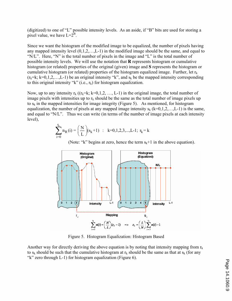
Now, up to any intensity rk ((rk=k; k=0,1,2, …, L-1) in the original image, the total number of

image pixels with intensities up to rk should be the same as the total number of image pixels up

to sk in the mapped intensities for image integrity (Figure 5). As mentioned, for histogram

equalization, the number of pixels at any mapped image intensity sk (k=0,1,2,…,L-1) is the same,

and equal to “N/L”. Thus we can write (in terms of the number of image pixels at each intensity

level),

kr

R k k

i=0

Nn (i) = (s +1) : k=0,1,2,3,...,L-1; r = k

L

⎛ ⎞⎜ ⎟⎝ ⎠∑

(Note: “k” begins at zero, hence the term sk+1 in the above equation).

Figure 5. Histogram Equalization: Histogram Based

Another way for directly deriving the above equation is by noting that intensity mapping from rk

to sk should be such that the cumulative histogram at rk should be the same as that at sk (for any

“k” zero through L-1) for histogram equalization (Figure 6).

Page 14.1060.9

In the above, “N” is the total number of pixels in the given image, “L” is the total number of

possible intensity (gray) levels (possible intensity levels are 0, 1, 2, …, L-1), n(i) is the number

of image pixels in the (original) image with intensity “i” (here, “i” is a “running index” in the

above equation), rk is the original intensity “k”, and sk is the mapped intensity corresponding to

original intensity “k” (i.e., corresponding to rk). Note that the notation “r” is used to imply the

original (given) image and “s” to imply the modified image in the above.

Figure 6. Histogram Equalization: Cumulative-Histogram Based

Thus for example, n(128) stands for the number of image pixels with an intensity of 128 (in the

original image), r128 stands for intensity 128 in the original image (i.e., r128 = 128), and s128

stands for the mapped intensity of the original intensity 128 (which could be for example,

intensity 147 in which case s128 = 147). This would mean that all pixels in the original image

with a pixel intensity of 128 are mapped to an intensity of 147 in the modified image.

In the above equation, since n(i) is the number of image pixels having an intensity level of “i”,

we have n(i) = h(i) by the definition of a histogram. Therefore, the above equation can be

rewritten in terms of the histogram h(i) as,

kr

R k k

i=0

Nh (i) = (s +1) : k=0,1,2,3,...,L-1; r = k

L

⎛ ⎞⎜ ⎟⎝ ⎠∑

It should next be noted that intensity levels are discrete in digital images (they are integers in the

range 0 through “L-1”). Further, in order to maintain “informational integrity” of the image, all

image pixels with the same intensity in the original image cannot be assigned to different

intensities but be mapped to the same new value en masse. Thus, remapping image intensities in

an image for perfect histogram equalization will not be possible for digital images.

Thus, in a practical sense, what we would like to aim for is not a perfect equalization of the

mapped intensities, but something that would be close. Therefore, what we want is to map

intensity level rk (rk=k; k=0,1,2,…,L-1) to an intensity level sk such that up to sk (k=0,1,2,…,L-1)

in the modified image, the error (i.e., difference) (Δk) between the histogram of the resulting

mapped (modified) image and that of the equalized histogram is minimized. Of course in the

ideal case (perfect equalization), Δk would be zero. Therefore, it can be said that we want to map

Page 14.1060.10

a pixel intensity rk (rk=k; k = 0,1,2,…,L-1) in the original (given) image to an intensity sk (to be

determined) such that Δk in the equation below is minimized.

kr

k kk R

i=0

Nǻ = : k=0,1,2,3,...,L-1; r = k(s +1) - h (i)L

⎛ ⎞⎜ ⎟⎝ ⎠ ∑

Here, |…| represents the absolute value of what is within. By factoring out N/L and rewriting the

above equation, the above minimization can be easily modified to a minimization of the

following:

kr'k k kR

i=0

Lǻ = s - : k=0,1,2,3,...,L-1; r = kh (i) - 1N

⎛ ⎞⎛ ⎞⎜ ⎟⎜ ⎟⎜ ⎟⎝ ⎠⎝ ⎠∑

For any given rk, it is always possible to determine sk such that the above minimization is zero

(ideal minimization). This could be done by solving for sk after making Δ’k zero. It would yield

sk as,

kr

k R k

i=0

Ls = h (i) - 1 : k=0,1,2,3,...,L-1; r = k

N

⎛ ⎞⎜ ⎟⎝ ⎠∑

However in the above, sk (the mapped pixel intensity) is not guaranteed to be an integer (and, in

general it will not be an integer). But for digital images, pixel intensities are constraint to be

integers (0,1,2,…,L-1). Thus, it is self-evident from the minimization expression that for the best

possible minimization with this constraint, the mapped pixel intensity sk should be chosen as,

kr

k kR

i=0

Ls = round : k=0,1,2,3,...,L-1; r = kh (i) - 1

N

⎛ ⎞⎛ ⎞⎜ ⎟⎜ ⎟⎜ ⎟⎝ ⎠⎝ ⎠∑

From the above equation it is evident that for intensity levels in the original image from zero up

to the intensity level where the total number of image pixels with those intensities is less than

“N/L”, the expression would result in negatively mapped intensities (sk) (or to be precise, this is

up to the pixel intensity where the total number of pixels is less than “N/2L” when rounding is in

use, and sk would become -1 in this situation). However, for image intensities, sk is constraint to

be non-negative (intensities cannot be negative). Thus, sk in the rk−>sk mapping for histogram

equalization in terms of the intensity histogram of the original (given) image should be such that,

kr

k k

i=0

kk

k k

Ls' = h(i) - 1 : k=0,1,2,3,...,L-1; r = k

N

0 : s' <0s = : k=0,1,2,3,...,L-1

round(s' ) : s' ³0

⎫⎛ ⎞ ⎪⎜ ⎟ ⎪⎝ ⎠ ⎪⎬⎪⎧⎪⎨⎪⎩ ⎭

∑

By the definition of cumulative histogram, the summation in the above equation can be written

as the cumulative histogram at intensity “k” (i.e., Ck). Thus, in terms of the cumulative intensity

histogram of the original (given) image, the above can be written as,

Page 14.1060.11

k R k

kk

k k

Ls' = C (k) - 1 : k=0,1,2,3,...,L-1; r = k

N

0 : s' <0s = : k=0,1,2,3,...,L-1

round(s' ) : s' ³0

⎫⎛ ⎞⎜ ⎟ ⎪⎝ ⎠ ⎪

⎬⎧ ⎪⎨ ⎪⎩ ⎭

As a representational simplification, we can write the above mapping (either using the histogram

or the cumulative histogram based expression) for histogram equalization as given below, but

with the understanding that sk is adjusted to zero if the expression on the right hand side

evaluates to less than zero, and it is the rounded otherwise:

kr

k R k

i=0

k R k

Ls = h (i) - 1 : k=0,1,2,3,...,L-1; r = k (w.r.t. Histogram)

N

Ls = C (k) - 1 : k=0,1,2,3,...,L-1; r = k (w.r.t. CumulativeHistogram)

N

⎛ ⎞⎜ ⎟⎝ ⎠

⎛ ⎞⎜ ⎟⎝ ⎠

∑

The above equation(s) defines the mapping rk−>sk from an original intensity (rk) (rk=k; k=0,1,2,

…, L-1) (i.e., R) to a mapped intensity (sk) (i.e., S) for (best) histogram equalization. As we had

noted, this will not result in a perfectly equalized histogram for the so modified image, but would

be as close to an equalized histogram as possible that a digital image would permit while

retaining image integrity (pixel ranking order).

Figure 7. Histogram Equalization: Lookup Table and Input-Output Mapping

Also, it can be easily shown that for k = L-1, we get sk = rk; that is, the L-1 (max) intensity level

will always map to L-1 (the max intensity level). Further, if 2 1k kr r> , then we get 2 1k ks s≥ as it

ought to be for any meaningful “image structure preserving” intensity mapping of an image.

Thus as required and expected, the histogram equalization mapping is single-valued and

monotonically increasing; it is also non-linear.

Page 14.1060.12

Based on the above, a lookup table (LUTRS) for histogram equalization can be created. It could

thereafter be used for mapping each pixel intensity value in the original image to a new intensity

value (Figure 7, and Figure 4) for histogram equalization of the original image.

3.5 Histogram Equalization: Summary of Steps

The entire technique (steps) for histogram equalization (as discussed above) could be

summarized and stated as follows:

Step 1: Compute the intensity histogram and/or cumulative intensity histogram of the original

image. This will give us the number of pixels at each intensity level, or the cumulative number

of pixels having an intensity up to or below any given intensity level in the original image. Also,

determine the total number of image pixels in the given (original) image.

Step 2: Compute the (rk−>sk) lookup table (LUTRS) that would histogram-equalize the original

image. This can be done using either the histogram based equalization equation or the

cumulative histogram based equalization equation given below (the histogram equalization

mapping transformation – developed earlier), with the understanding that sk is adjusted to zero if

the expression on the right hand side evaluates to less than zero, and it is the rounded otherwise.

kr

k R k

i=0

k R k

Ls = h (i) - 1 : k=0,1,2,3,...,L-1; r = k (w.r.t. Histogram)

N

Ls = C (k) - 1 : k=0,1,2,3,...,L-1; r = k (w.r.t. CumulativeHistogram)

N

⎛ ⎞⎜ ⎟⎝ ⎠

⎛ ⎞⎜ ⎟⎝ ⎠

∑

Step 3: Using the above mapping transformation (LUTRS), transform the original image to a

histogram equalized image using the intensity transformation S=Intensity_Transform(R, LUTRS)

where R is the input image and S is the output (modified input) image with LUT being the input-

to-output mapping lookup table

Step 4 (Optional): Display (i) the original image, its histogram, and its cumulative histogram,

(ii) the modified image, its histogram, and its cumulative histogram, and (iii) the mapping

function (as a graph).

4.0 A MATLAB GUIDE based GUI Tool for Teaching and Demonstration

4.1 The MATLAB m-Function Files for Demonstrations

Having developed the background and theory to be used for teaching histogram equalization, it

was best to visually demonstrate and teach histogram equalization through demonstrating the

various steps involved, and the effects of histogram equalization on a variety of images – all of

these to supplement and complement the lectures and to aid understanding.

Page 14.1060.13

In order to accomplish this, various simple MATLAB m-function files were first modularly

developed and used by the author for initial demonstrations. These m-functions were developed

for the following purposes: (i) reading and displaying any given image, (ii) computing and

displaying the given image’s intensity histogram, (iii) computing and displaying the given

image’s cumulative intensity histogram, (iv) histogram equalizing the given image to produce a

histogram equalized image, (v) displaying the histogram equalized image, (vi) computing and

displaying the histogram equalized image’s intensity histogram, (vii) computing and displaying

the histogram equalized image’s cumulative intensity histogram, and (viii) computing and

displaying the mapping function that resulted by the histogram equalization function which

brought about the histogram equalization of the given image. It should be noted that some of the

above mentioned functions are actually combined into a single function with their differences

incorporated as parameters to the respective functions (but is described as above for clarity).

Special allowances were incorporated into these m-functions to suitably handle grayscale as well

as color images (after having properly interpreted the meaning of histogram equalization under

these circumstances).

4.2 The MATLAB GUIDE based GUI for Demonstrations

A MATLAB GUIDE based GUI tool was subsequently developed by the author by quickly

integrating into a common GUI these m-functions that were first developed and used for teaching

purposes. This was to make the demonstrations quick and convenient. The user-interface of this

GUI tool is shown in Figure 8. The interface and organization of this tool was based on making

teaching, learning, and studying histogram equalization as painless as possible.

As can be seen (Figure 8), the main GUI window has a pushbutton to select the current directory

(bottom left), and another to select an image file from this directory (bottom left). Upon clicking

any of these two buttons, the respective popup window (not shown) appears to enable selecting

the directory and the image file from that directory. Upon selecting an image file (with a file

type supported by MATLAB), the following are immediately computed and displayed in their

respective windows within this main GUI window: (1) (a) the original image, (b) its histogram,

and (c) its cumulative histogram; and (2) (a) the histogram equalized image, (b) its histogram,

and (c) its cumulative histogram.

In the histogram windows (of both the original and equalized), a horizontal line is plotted

showing the expected (ideal) equalized value (N/L) for the image. Its numerical value too is

given (bottom center). Similarly, in the cumulative histogram windows (both original and

equalized), a linear graph is plotted showing the expected (ideal) cumulative equalized-histogram

values. These are provided for comparison of expected and actual values of the histograms and

cumulative histograms.

Clicking the “Image” pushbutton (top row, left of main GUI) will result in displaying the original

image and the histogram equalized image in a separate full screen sub-window (for enlarged

view of the images) (Figure 9). Similarly, clicking the “Histogram” button (top row, middle of

main GUI) will result in displaying the histogram of the original image and that of the histogram

equalized image in a separate full screen sub-window (for enlarged/ horizontally stretched view

of the histograms) (Figure 10). Clicking the “Cumulative Histogram” button (top row, right of

Page 14.1060.14

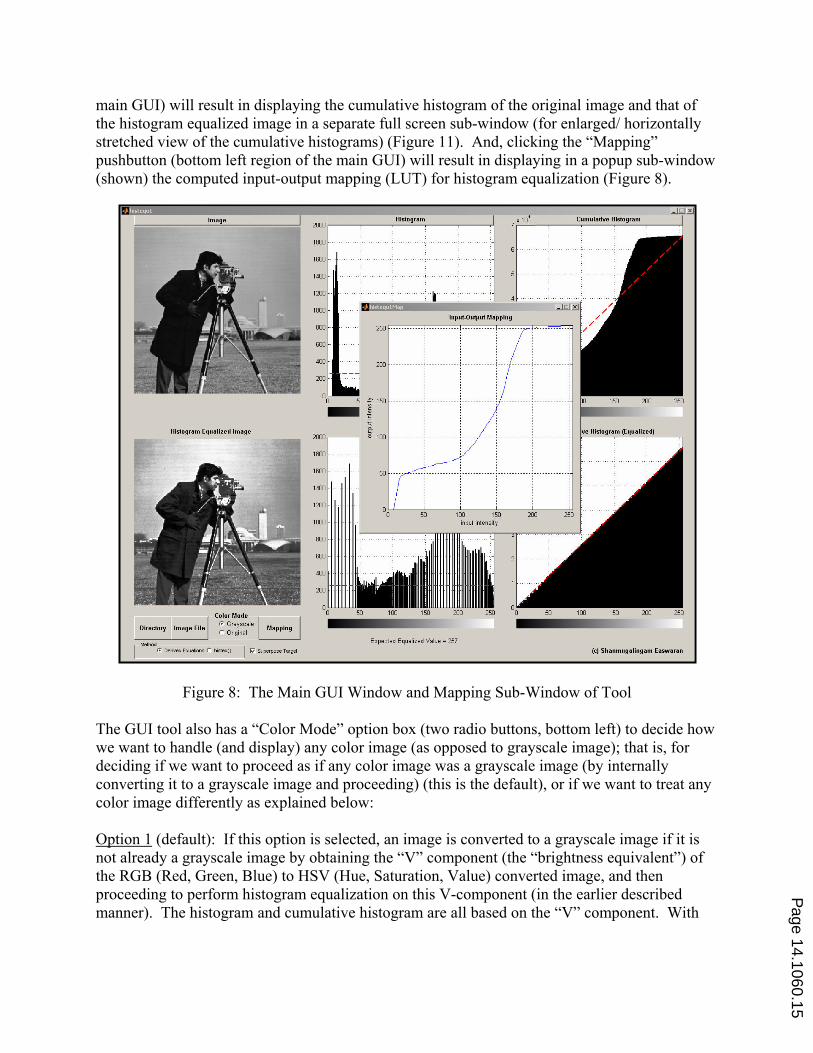
main GUI) will result in displaying the cumulative histogram of the original image and that of

the histogram equalized image in a separate full screen sub-window (for enlarged/ horizontally

stretched view of the cumulative histograms) (Figure 11). And, clicking the “Mapping”

pushbutton (bottom left region of the main GUI) will result in displaying in a popup sub-window

(shown) the computed input-output mapping (LUT) for histogram equalization (Figure 8).

Figure 8: The Main GUI Window and Mapping Sub-Window of Tool

The GUI tool also has a “Color Mode” option box (two radio buttons, bottom left) to decide how

we want to handle (and display) any color image (as opposed to grayscale image); that is, for

deciding if we want to proceed as if any color image was a grayscale image (by internally

converting it to a grayscale image and proceeding) (this is the default), or if we want to treat any

color image differently as explained below:

Option 1 (default): If this option is selected, an image is converted to a grayscale image if it is

not already a grayscale image by obtaining the “V” component (the “brightness equivalent”) of

the RGB (Red, Green, Blue) to HSV (Hue, Saturation, Value) converted image, and then

proceeding to perform histogram equalization on this V-component (in the earlier described

manner). The histogram and cumulative histogram are all based on the “V” component. With

Page 14.1060.15

this option, the images displayed are the equivalent grayscale images regardless of their original

chromatic condition.

Figure 9: The Image Sub-GUI (popup) Window

Figure 10: The Histogram Sub-GUI (popup) Window

Option 2: If this option is selected, in case of a color image the V-component of the RGB to

HSV converted image is obtained, a histogram equalization (as above) is performed on this V-

component (and only on the V-component), and then using this histogram equalized V-

component and the original H and S-components the histogram equalized color image is

Page 14.1060.16

obtained via HSV to RGB conversion. The images displayed in this case are the original image

(in color if the original was a color image) and the histogram-equalized image (in color if the

original was a color image). That is, the images are displayed in their native chromatic form.

The GUI tool also has a “Matching Method” option box (two radio buttons, bottom left) that

enables one to choose which method is to be employed in the histogram equalization process for

comparing the results of histogram equalization using Option 1: “Derived Equations (by

Author)”, and Option 2: “MATLAB histeq() Function”.

4.3 The Usage of the Demonstration Tools

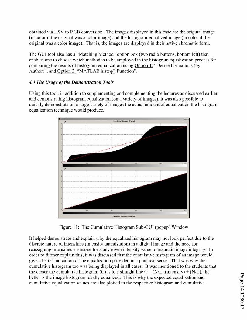
Using this tool, in addition to supplementing and complementing the lectures as discussed earlier

and demonstrating histogram equalization (on a variety of images), it was also possible to

quickly demonstrate on a large variety of images the actual amount of equalization the histogram

equalization technique would produce.

Figure 11: The Cumulative Histogram Sub-GUI (popup) Window

It helped demonstrate and explain why the equalized histogram may not look perfect due to the

discrete nature of intensities (intensity quantization) in a digital image and the need for

reassigning intensities en-masse for a any given intensity value to maintain image integrity. In

order to further explain this, it was discussed that the cumulative histogram of an image would

give a better indication of the equalization provided in a practical sense. That was why the

cumulative histogram too was being displayed in all cases. It was mentioned to the students that

the closer the cumulative histogram (C) is to a straight line C = (N/L).(intensity) + (N/L), the

better is the image histogram ideally equalized. This is why the expected equalization and

cumulative equalization values are also plotted in the respective histogram and cumulative

Page 14.1060.17

histogram windows. These helped with understanding and appreciating histogram equalization

in the real sense.

It should be noted that the histogram equalization results obtained using the equation derived and

discussed by the author also matched very closely (hardly different if at all) to those obtained

using the MATLAB function histeq() for histogram equalization.

5.0 The Effectiveness of the Teaching and GUI Tool

In order to evaluate the effectiveness of the provided teaching framework and methodology,

theory and derived equations, the histogram-equalization process, and MATLAB GUIDE based

GUI tool demonstrations, the following was done by the author. This was done for the spring

2006 semester with six computer-engineering as well as computer-science undergraduate

students in the digital image processing class, and for the spring 2005 semester with nine

computer-engineering undergraduate students in the digital signal processing class (which had an

image processing a sub-area within the course).

In these courses, the students were initially taught histogram equalization in a general way (as

described in the standard and other textbooks1-9 and not as described in this paper). It should be

noted that it was the considerable difficulty I was having in teaching this subtopic to students as

described in the standard and other textbooks (and their poor performance in corresponding

homework assignments) that made me develop and use what was described in this paper.

It should also be noted that prior to teaching histogram equalization, the students had been taught

intensity histograms and cumulative intensity histograms as applied to digital images, contrast

enhancements through point processing using contrast stretching, and image intensity

transformations using lookup tables (LUTs). They have also had MATLAB homework exercises

based on these.

The students were also asked to refer to the course textbook and/ or other textbooks in image

processing (most of which were available in the university library) to histogram equalize a given

grayscale image. They were given two homework assignments to work on and submit. As

always, they were allowed to discuss with the instructor finer points they had difficulties with.

They were also asked to write down difficulties they have had while working through the

homework assignments. The homework problems were essentially as described below:

(1) The students were given a simple artificial “image” (of size 8x8, and with eight quantization

levels) and was asked to manually perform histogram equalization. In a different situation, they

were told the number of pixels that had a certain intensity level for each of the possible eight

intensity levels, i.e. its histogram, instead of giving them image intensity values). The idea

behind this manual computation assignment was the hope of providing students with insights as

they worked through the problem, and also to determine if they had understood the concepts

involved. This was also to enable the students to subsequently write a MATLAB program to

perform histogram equalization of a given real image. They were asked to show the histogram

and the cumulative histogram of the original image, the histogram and the cumulative histogram

Page 14.1060.18

of the “histogram equalized” image, and the intensity mapping needed to go from the original

image to the histogram equalized image.

(2) The students were asked to perform histogram equalization on a MATLAB provided image

(image ‘pout.tif’, size 240 by 291, gray levels 256). They were asked to show the original

image, the histogram and the cumulative histogram of the original image; the histogram

equalized image, the histogram and the cumulative histogram of the “histogram equalized”

image; and the intensity mapping to map the intensities from the original image to the histogram

equalized image intensities. They were further asked to compare their results to that obtained

using the MATLAB histeq() function.

After giving the students a week to work on these assignments, because of the difficulty all the

students were having, they were taught histogram equalization as described in this paper. They

were then given the same assignments to work on again and submit.

Before teaching histogram equalization as described in this paper, the students were frustrated

that they could hardly understand the background/ theory and technique described in the

textbooks or in the internet, and thus they were hardly able to proceed with the problem itself

(none of the students were able to make progress with the problems in any meaningful way).

They complained that the available materials1-9

(textbooks, reference books, internet searches)

were mathematically too advanced and complex to understand or was not clear, or that they do

not have a clear background on probability/ probability distributions or integral calculus (all of

the texts use these advanced mathematical concepts to discuss histogram equalization) to

properly understand the process of histogram equalization, or that the procedure to follow was

not clear or clearly explained in the texts.

However, after teaching histogram equalization in the manner described in this paper, they all

had a clear understanding of histogram equalization. The student solutions, comments, survey

results indicate that they understood histogram equalization quite well. They all said (at an

individual interview with each student discussing their work) that they were able to completely

understand the concepts, theory and technique behind histogram equalization.

In order to evaluate the effectiveness of the teaching of histogram equalization as stated above,

the homework assignment scores of the students (on this subtopic) were scaled to 10 points and

the statistics were computed for the 12 (of the total of 15) students who had attended all the

lectures when this subtopic was taught, with and without the methodology described. The

statistics for the pre and post-tests were follows: For the pre-test, the students were having so

much difficulty in progressing with the assignments that their assignments were not graded as

such. For the post-test, the average score was 8.85 with a standard deviation of 1.30.

The students were also given an evaluation form after they had been taught using the

methodology described. Among other questions, they were asked how strongly they agreed

(from “very strongly” = 5, to “strongly disagree” = 1) that their learning and understanding of

this subtopic had considerably improved based on the methodology, developments and

explanations, and demonstrations shown using the MATLAB-tool developed. Only the twelve

students who had attended all the lectures when this topic was taught with and without the

Page 14.1060.19

methodology described, were asked to provide their feedback: 10 strongly agreed and 2 agreed.

Their comments too indicated similarly.

Though the results indicate significant improvements in student learning when taught using the

methodology described in this paper, more student performance data and more careful testing

and comparison strategies that are also practical may be needed for obtaining mathematically

meaningful statistical measures and to draw statistically strong conclusions (if needed).

6.0 Summary and Conclusion

In this paper, the following that were derived/ developed/ implemented and used by the author

for teaching histogram equalization in digital image processing were described: (i) a simpler

teaching-learning framework and background (methodology), (ii) a simple and clear theory and

the necessary derived equations, (iii) a clear process for histogram equalization, and (iv) a

MATLAB GUIDE based GUI tool/ m-function files for visual demonstrations. Student

performance before and after teaching this subtopic as described in this paper indicated that

student learning and understanding was greatly simplified and improved. The teaching too was

made considerably simpler at a greater level of rigor.

Bibliography

1. Gonzalez, Woods, “Digital Image Processing”, Second Edition, Prentice Hall (2002)

2. Gonzalez, Woods, Eddins, “Digital Image Processing with Matlab”, Prentice Hall (2006)

3. Castleman, “Digital Image Processing”, Prentice Hall (1996)

4. Bose, “Digital Signal and Image Processing”, John Wiley & Sons (November 2003)

5. McAndrew, “Introduction to Digital Image Processing with Matlab”, Thomson Course Technology (2004)

6. Hall, “Computer Image Processing and Recognition”, Academic Press (1979)

7. Petrou, Bosdogianni, “Image Processing The Fundamentals”, Fourth Edition, John Wiley & Sons (April 2004)

8. Acharya, Ray, “Image Processing Principles and Applications”, Wiley-Interscience (2005)

9. Nixon, Aguado, “Feature Extraction & Image Processing”, Newnes (2002)

10. “MATLAB GUIDE User Manual”, MathWorks Inc.

Page 14.1060.20